introduction to choosing the correct statistical test + tests for continuous outcomes i
Post on 19-Dec-2015
242 views
TRANSCRIPT
Introduction to choosing the correct statistical test
+Tests for Continuous
Outcomes I
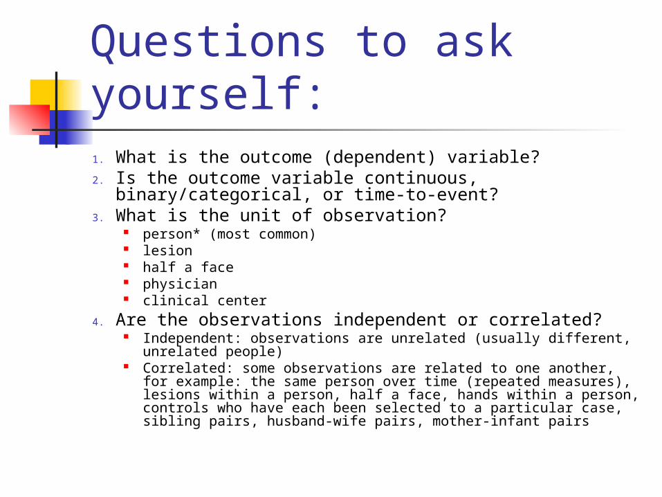
Questions to ask yourself:1. What is the outcome (dependent) variable?2. Is the outcome variable continuous, binary/categorical,
or time-to-event? 3. What is the unit of observation?
person* (most common) lesion half a face physician clinical center
4. Are the observations independent or correlated? Independent: observations are unrelated (usually different,
unrelated people) Correlated: some observations are related to one another, for
example: the same person over time (repeated measures), lesions within a person, half a face, hands within a person, controls who have each been selected to a particular case, sibling pairs, husband-wife pairs, mother-infant pairs
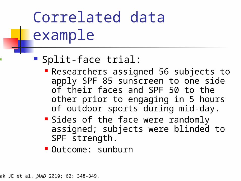
Correlated data example Split-face trial:
Researchers assigned 56 subjects to apply SPF 85 sunscreen to one side of their faces and SPF 50 to the other prior to engaging in 5 hours of outdoor sports during mid-day.
Sides of the face were randomly assigned; subjects were blinded to SPF strength.
Outcome: sunburn
Russak JE et al. JAAD 2010; 62: 348-349.
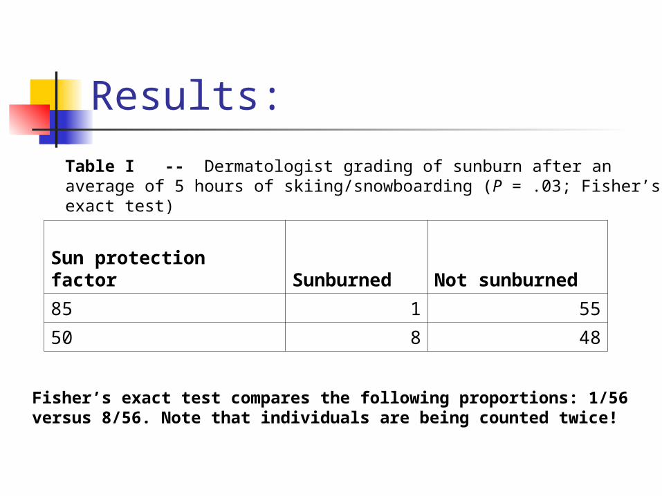
Results:
Table I -- Dermatologist grading of sunburn after an average of 5 hours of skiing/snowboarding (P = .03; Fisher’s exact test)
Sun protection factor Sunburned Not sunburned
85 1 55
50 8 48
Fisher’s exact test compares the following proportions: 1/56 versus 8/56. Note that individuals are being counted twice!
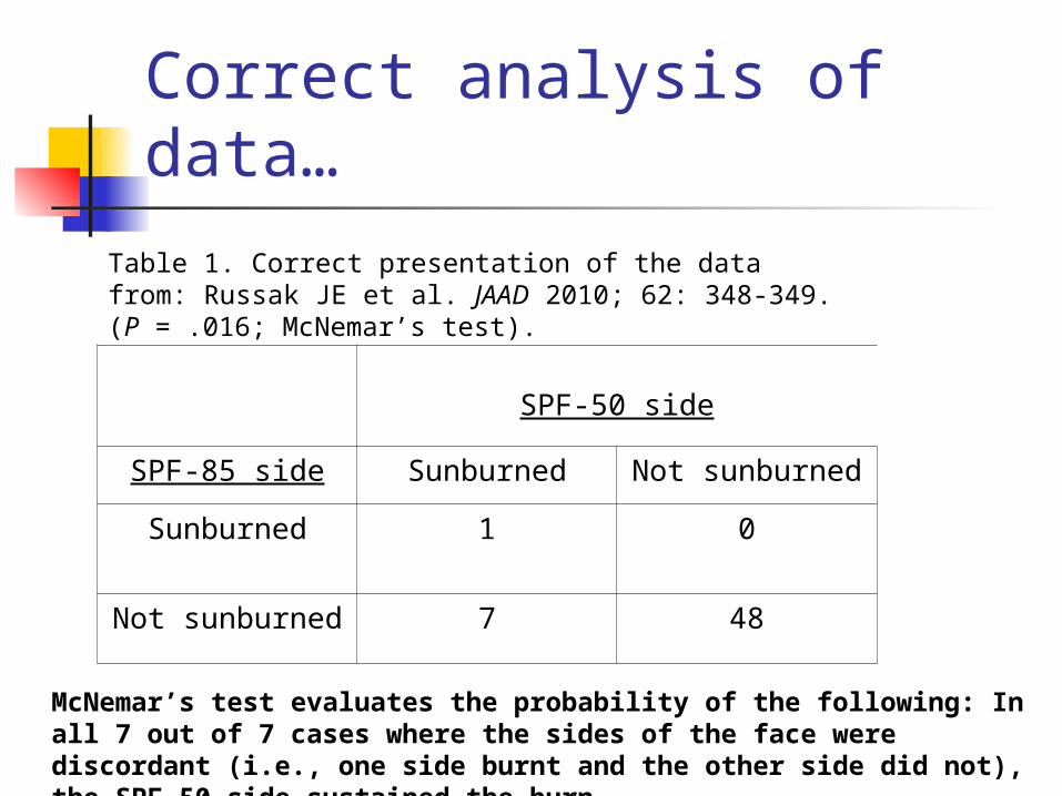
Correct analysis of data…
Table 1. Correct presentation of the data from: Russak JE et al. JAAD 2010; 62: 348-349. (P = .016; McNemar’s test).
SPF-50 side
SPF-85 side Sunburned Not sunburned
Sunburned 1 0
Not sunburned 7 48
McNemar’s test evaluates the probability of the following: In all 7 out of 7 cases where the sides of the face were discordant (i.e., one side burnt and the other side did not), the SPF 50 side sustained the burn.
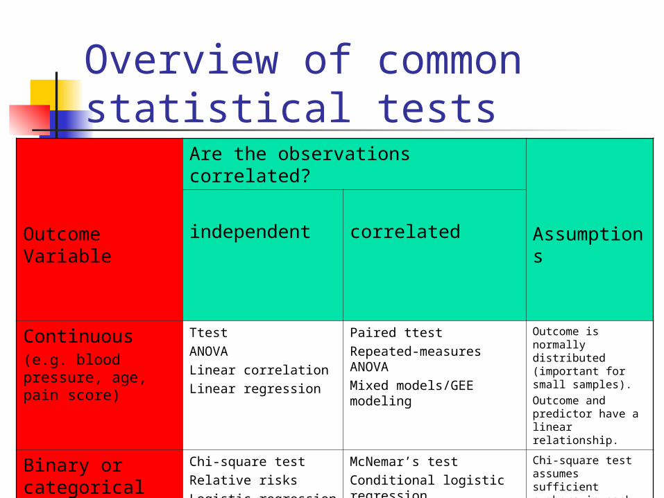
Overview of common statistical tests
Outcome Variable
Are the observations correlated?
Assumptions
independent correlated
Continuous(e.g. blood pressure, age, pain score)
TtestANOVALinear correlationLinear regression
Paired ttestRepeated-measures ANOVAMixed models/GEE modeling
Outcome is normally distributed (important for small samples).Outcome and predictor have a linear relationship.
Binary or categorical(e.g. breast cancer yes/no)
Chi-square test Relative risksLogistic regression
McNemar’s testConditional logistic regressionGEE modeling
Chi-square test assumes sufficient numbers in each cell (>=5)
Time-to-event(e.g. time-to-death, time-to-fracture)
Kaplan-Meier statisticsCox regression
n/a Cox regression assumes proportional hazards between groups
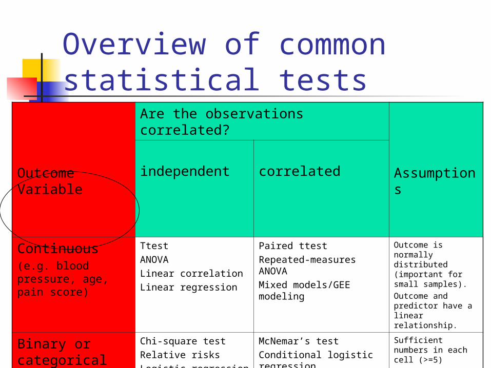
Overview of common statistical tests
Outcome Variable
Are the observations correlated?
Assumptions
independent correlated
Continuous(e.g. blood pressure, age, pain score)
TtestANOVALinear correlationLinear regression
Paired ttestRepeated-measures ANOVAMixed models/GEE modeling
Outcome is normally distributed (important for small samples).Outcome and predictor have a linear relationship.
Binary or categorical(e.g. breast cancer yes/no)
Chi-square test Relative risksLogistic regression
McNemar’s testConditional logistic regressionGEE modeling
Sufficient numbers in each cell (>=5)
Time-to-event(e.g. time-to-death, time-to-fracture)
Kaplan-Meier statisticsCox regression
n/a Cox regression assumes proportional hazards between groups

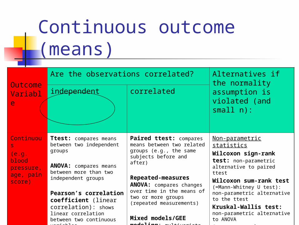
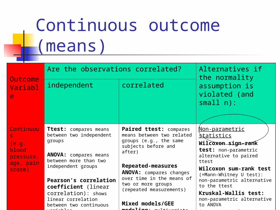
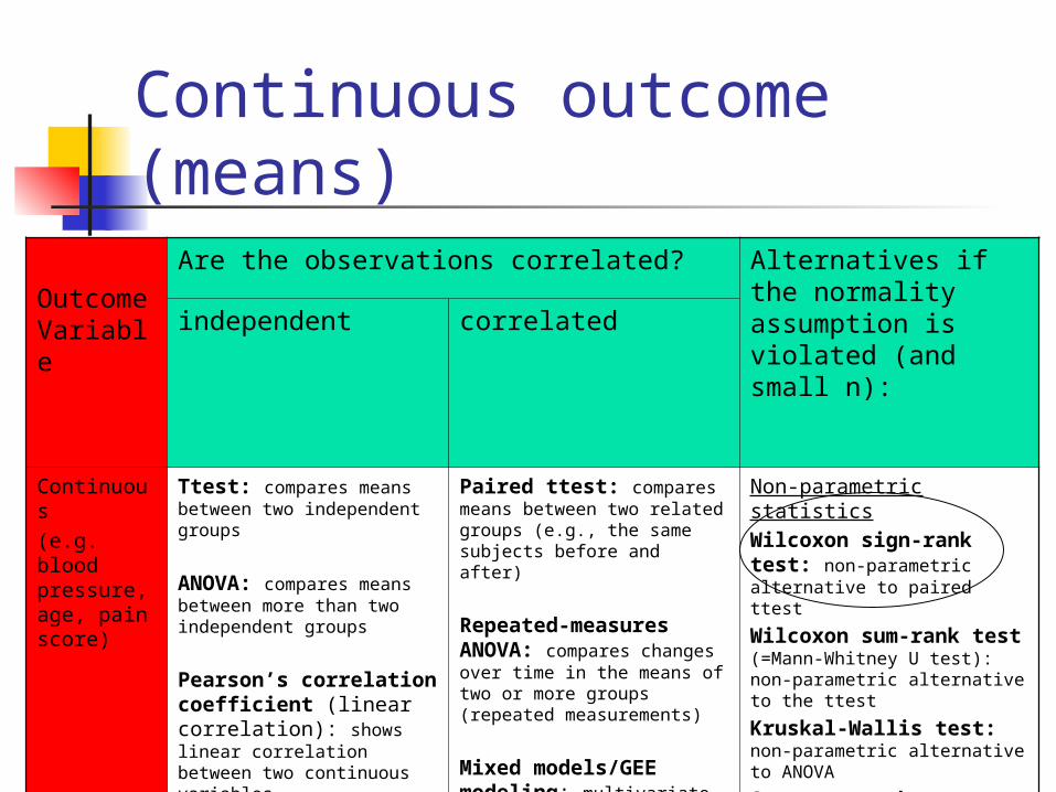
Continuous outcome (means)
Outcome Variable
Are the observations correlated? Alternatives if the normality assumption is violated (and small n):
independent correlated
Continuous(e.g. blood pressure, age, pain score)
Ttest: compares means between two independent groups
ANOVA: compares means between more than two independent groups
Pearson’s correlation coefficient (linear correlation): shows linear correlation between two continuous variables
Linear regression: multivariate regression technique when the outcome is continuous; gives slopes or adjusted means
Paired ttest: compares means between two related groups (e.g., the same subjects before and after)
Repeated-measures ANOVA: compares changes over time in the means of two or more groups (repeated measurements)
Mixed models/GEE modeling: multivariate regression techniques to compare changes over time between two or more groups
Non-parametric statisticsWilcoxon sign-rank test: non-parametric alternative to paired ttest
Wilcoxon sum-rank test (=Mann-Whitney U test): non-parametric alternative to the ttest
Kruskal-Wallis test: non-parametric alternative to ANOVA
Spearman rank correlation coefficient: non-parametric alternative to Pearson’s correlation coefficient
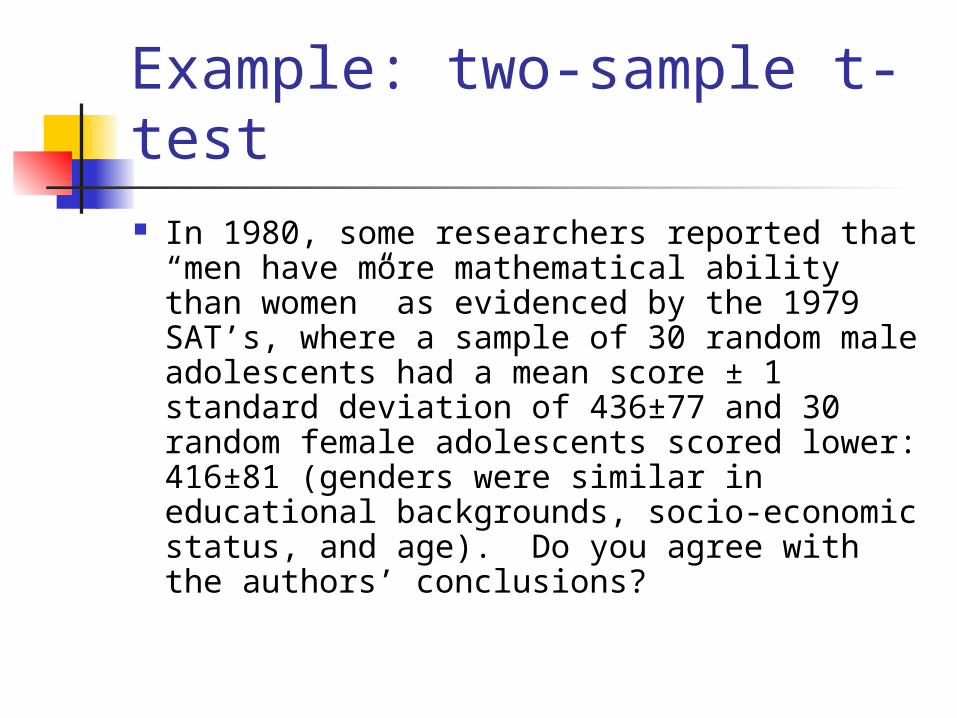
Example: two-sample t-test In 1980, some researchers reported that
“men have more mathematical ability than women” as evidenced by the 1979 SAT’s, where a sample of 30 random male adolescents had a mean score ± 1 standard deviation of 436±77 and 30 random female adolescents scored lower: 416±81 (genders were similar in educational backgrounds, socio-economic status, and age). Do you agree with the authors’ conclusions?
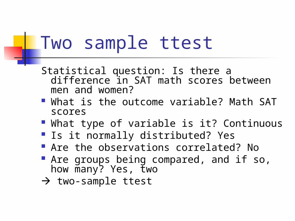
Two sample ttestStatistical question: Is there a difference in
SAT math scores between men and women?
What is the outcome variable? Math SAT scores
What type of variable is it? Continuous Is it normally distributed? Yes Are the observations correlated? No Are groups being compared, and if so,
how many? Yes, two two-sample ttest
Two-sample ttest mechanics…
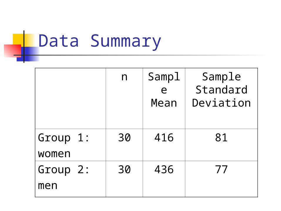
Data Summary
n Sample
Mean
Sample Standard Deviation
Group 1:women
30 416 81
Group 2:men
30 436 77
Two-sample t-test
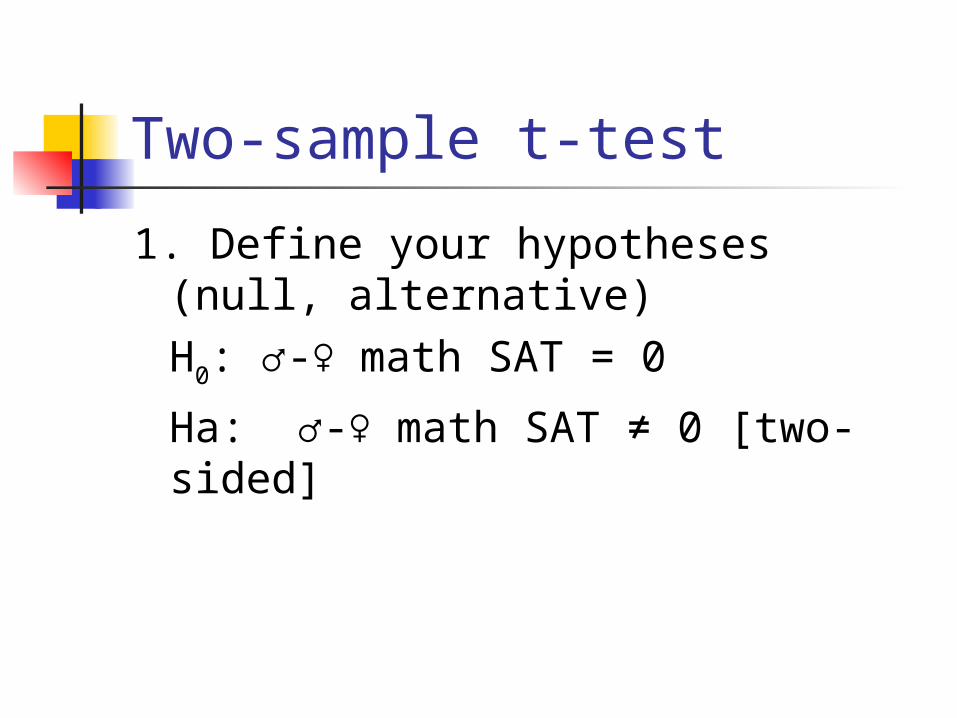
1. Define your hypotheses (null, alternative)H0: ♂-♀ math SAT = 0
Ha: ♂-♀ math SAT ≠ 0 [two-sided]
Two-sample t-test
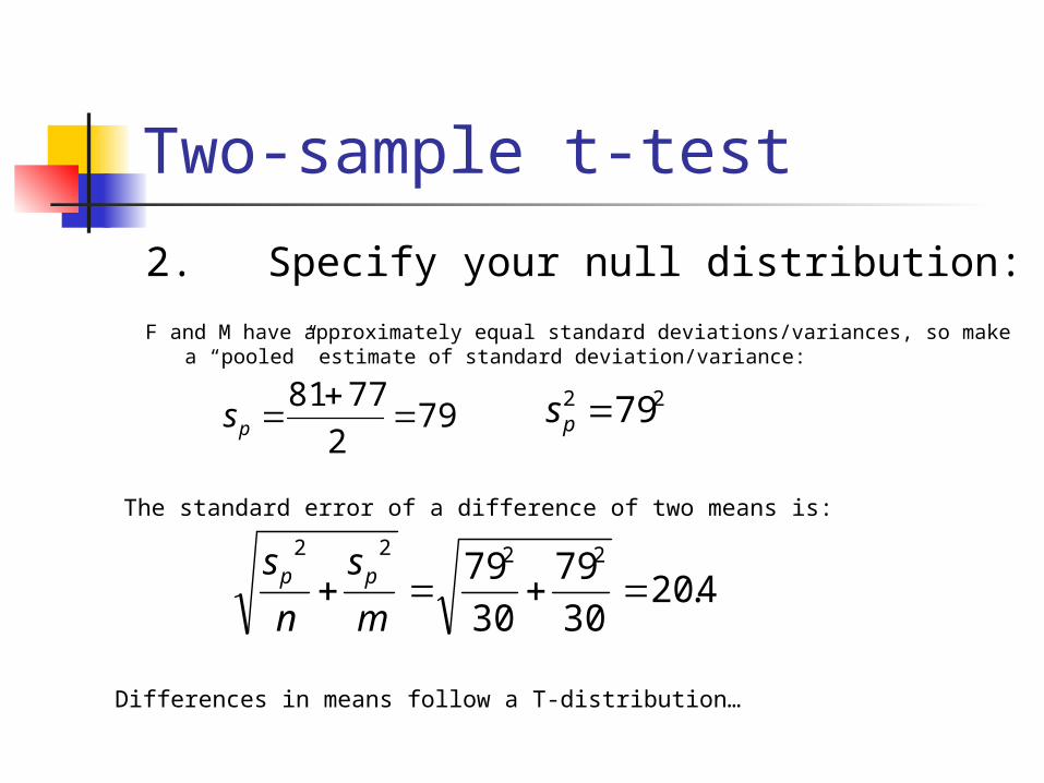
2. Specify your null distribution:
F and M have approximately equal standard deviations/variances, so make a “pooled” estimate of standard deviation/variance:
792
7781
ps
4.2030
79
30
79 2222
m
s
n
s pp
The standard error of a difference of two means is:
Differences in means follow a T-distribution…
22 79ps
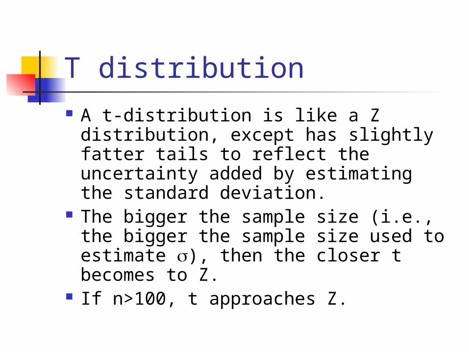
T distribution A t-distribution is like a Z distribution,
except has slightly fatter tails to reflect the uncertainty added by estimating the standard deviation.
The bigger the sample size (i.e., the bigger the sample size used to estimate ), then the closer t becomes to Z.
If n>100, t approaches Z.
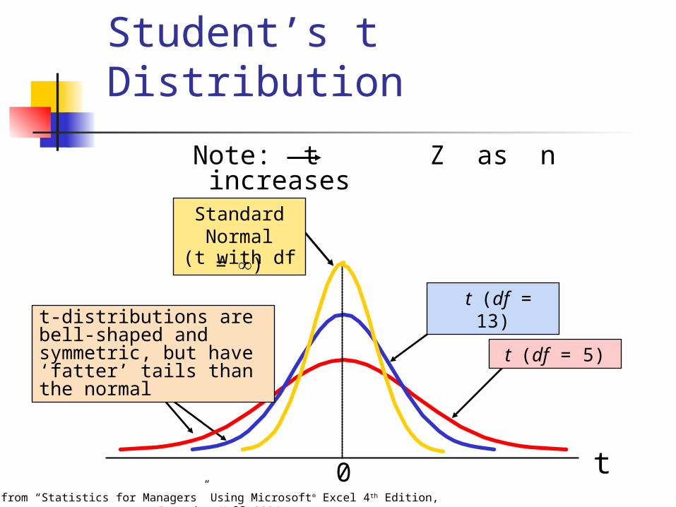
Student’s t Distribution
t0
t (df = 5)
t (df = 13)t-distributions are bell-shaped and symmetric, but have ‘fatter’ tails than the normal
Standard Normal
(t with df = )
Note: t Z as n increases
from “Statistics for Managers” Using Microsoft® Excel 4th Edition, Prentice-Hall 2004
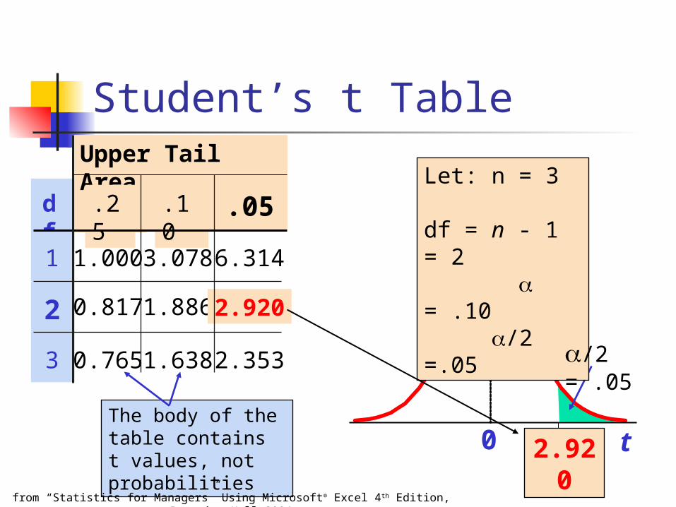
Student’s t TableUpper Tail Area
df .25 .10 .05
1 1.000 3.078 6.314
2 0.817 1.886 2.920
3 0.765 1.638 2.353
t0 2.920The body of the table contains t values, not probabilities
Let: n = 3 df = n - 1 = 2 = .10 /2 =.05
/2 = .05
from “Statistics for Managers” Using Microsoft® Excel 4th Edition, Prentice-Hall 2004
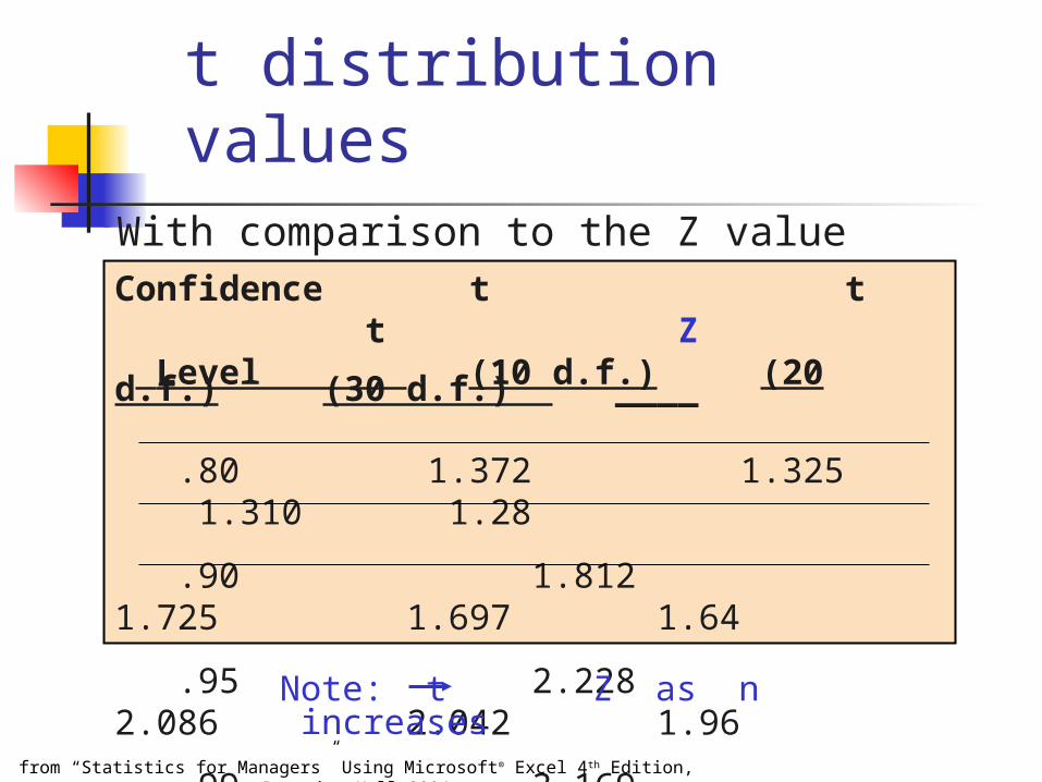
t distribution valuesWith comparison to the Z value
Confidence t t t Z Level (10 d.f.) (20 d.f.) (30 d.f.) ____
.80 1.372 1.325 1.310 1.28
.90 1.812 1.725 1.697 1.64
.95 2.228 2.086 2.042 1.96
.99 3.169 2.845 2.750 2.58
Note: t Z as n increases
from “Statistics for Managers” Using Microsoft® Excel 4th Edition, Prentice-Hall 2004
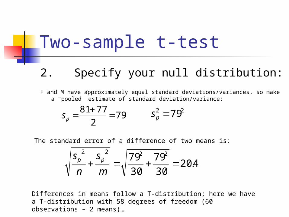
Two-sample t-test
2. Specify your null distribution:
F and M have approximately equal standard deviations/variances, so make a “pooled” estimate of standard deviation/variance:
792
7781
ps
4.2030
79
30
79 2222
m
s
n
s pp
The standard error of a difference of two means is:
Differences in means follow a T-distribution; here we have a T-distribution with 58 degrees of freedom (60 observations – 2 means)…
22 79ps
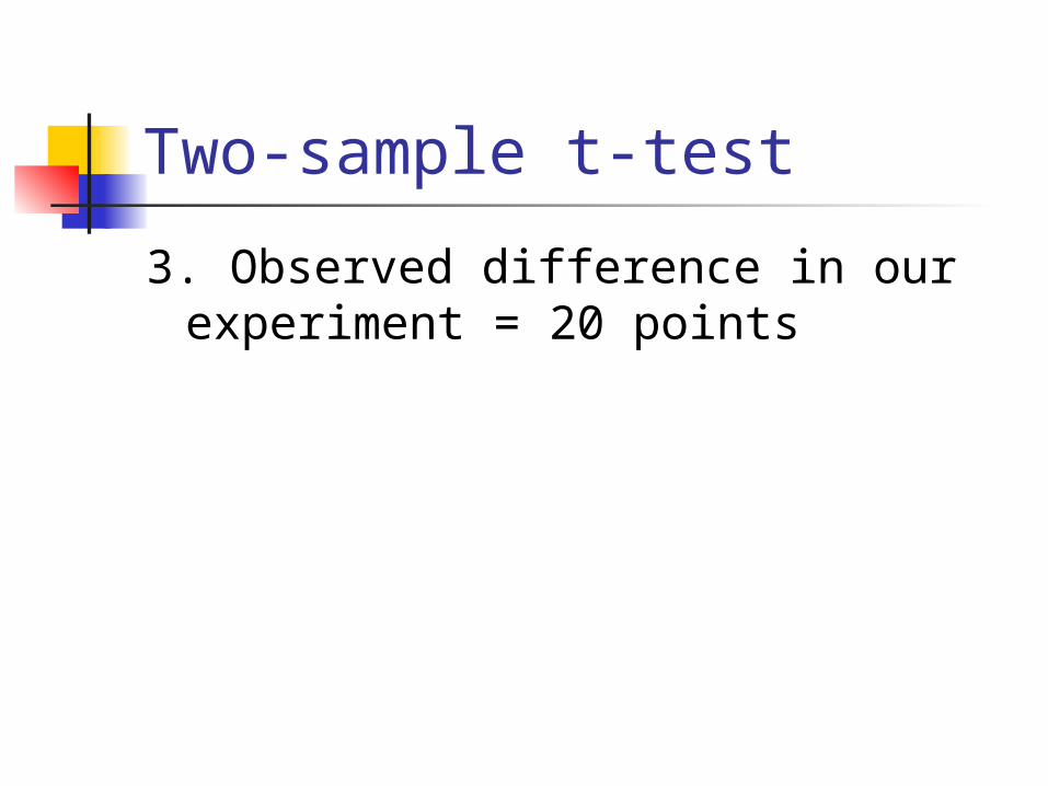
Two-sample t-test
3. Observed difference in our experiment = 20 points
Two-sample t-test
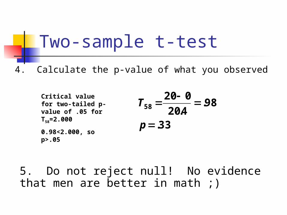
4. Calculate the p-value of what you observed
33.
98.4.20
02058
p
T
5. Do not reject null! No evidence that men are better in math ;)
Critical value for two-tailed p-value of .05 for T58=2.000
0.98<2.000, so p>.05
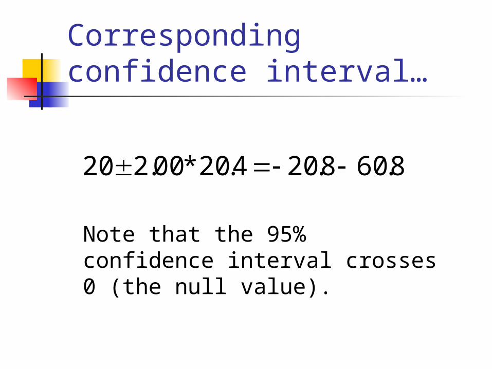
Corresponding confidence interval…
8.608.204.20*00.220
Note that the 95% confidence interval crosses 0 (the null value).
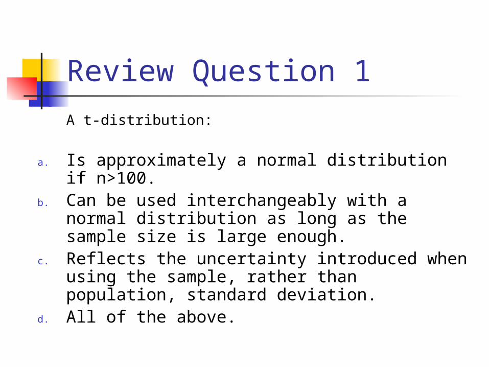
Review Question 1
A t-distribution:
a. Is approximately a normal distribution if n>100.
b. Can be used interchangeably with a normal distribution as long as the sample size is large enough.
c. Reflects the uncertainty introduced when using the sample, rather than population, standard deviation.
d. All of the above.
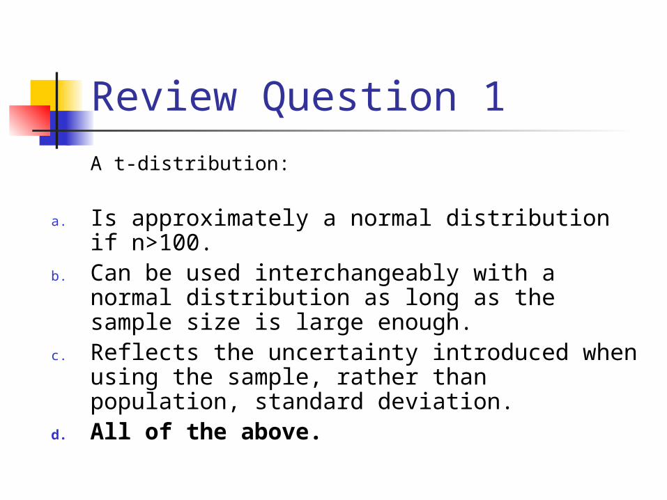
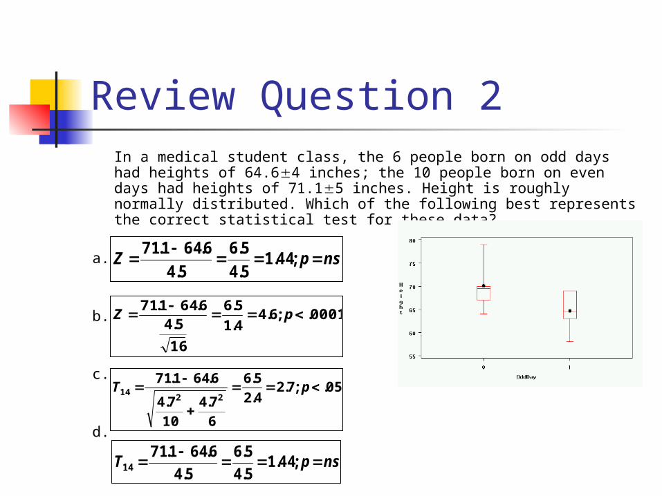
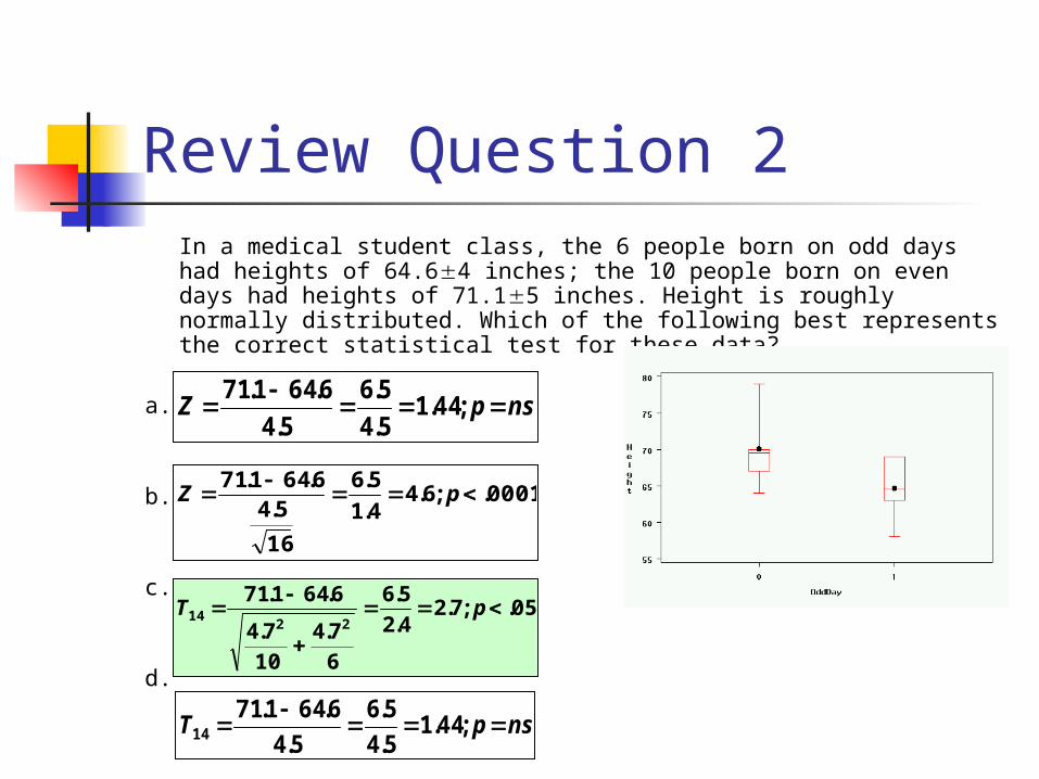
Review Question 2In a medical student class, the 6 people born on odd days had heights of 64.64 inches; the 10 people born on even days had heights of 71.15 inches. Height is roughly normally distributed. Which of the following best represents the correct statistical test for these data?
a.
b.
c.
d.
nspZ
;44.15.4
5.6
5.4
6.641.71
0001.;6.44.1
5.6
16
5.46.641.71
pZ
05.;7.24.2
5.6
6
7.4
10
7.4
6.641.7122
14
pT
nspT
;44.15.4
5.6
5.4
6.641.7114

Continuous outcome (means)
Outcome Variable
Are the observations correlated? Alternatives if the normality assumption is violated (and small n):
independent correlated
Continuous(e.g. blood pressure, age, pain score)
Ttest: compares means between two independent groups
ANOVA: compares means between more than two independent groups
Pearson’s correlation coefficient (linear correlation): shows linear correlation between two continuous variables
Linear regression: multivariate regression technique when the outcome is continuous; gives slopes or adjusted means
Paired ttest: compares means between two related groups (e.g., the same subjects before and after)
Repeated-measures ANOVA: compares changes over time in the means of two or more groups (repeated measurements)
Mixed models/GEE modeling: multivariate regression techniques to compare changes over time between two or more groups
Non-parametric statisticsWilcoxon sign-rank test: non-parametric alternative to paired ttest
Wilcoxon sum-rank test (=Mann-Whitney U test): non-parametric alternative to the ttest
Kruskal-Wallis test: non-parametric alternative to ANOVA
Spearman rank correlation coefficient: non-parametric alternative to Pearson’s correlation coefficient
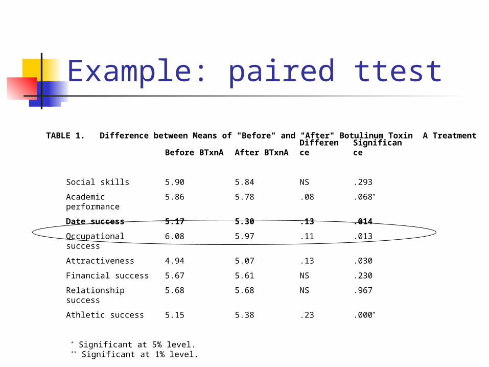
Example: paired ttest
Difference
Significance
Before BTxnA
After BTxnA
Social skills 5.90 5.84 NS .293
Academic performance
5.86 5.78 .08 .068*
Date success 5.17 5.30 .13 .014
Occupational success 6.08 5.97 .11 .013
Attractiveness 4.94 5.07 .13 .030
Financial success 5.67 5.61 NS .230
Relationship success 5.68 5.68 NS .967
Athletic success 5.15 5.38 .23 .000*
* Significant at 5% level. ** Significant at 1% level.
TABLE 1. Difference between Means of "Before" and "After" Botulinum Toxin A Treatment
Paired ttestStatistical question: Is there a difference in
date success after BoTox? What is the outcome variable? Date
success What type of variable is it? Continuous Is it normally distributed? Yes Are the observations correlated? Yes, it’s
the same patients before and after How many time points are being
compared? Two paired ttest
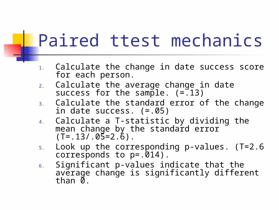
Paired ttest mechanics1. Calculate the change in date success score
for each person.2. Calculate the average change in date
success for the sample. (=.13)3. Calculate the standard error of the change in
date success. (=.05)4. Calculate a T-statistic by dividing the mean
change by the standard error (T=.13/.05=2.6).
5. Look up the corresponding p-values. (T=2.6 corresponds to p=.014).
6. Significant p-values indicate that the average change is significantly different than 0.
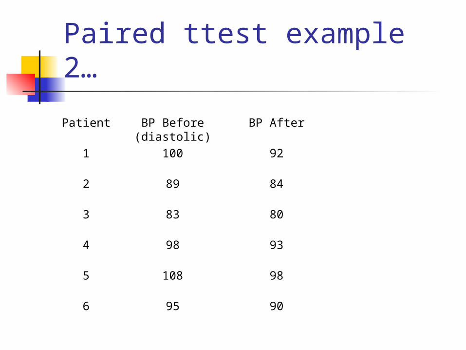
Paired ttest example 2…
Patient BP Before (diastolic) BP After
1 100 92
2 89 84
3 83 80
4 98 93
5 108 98
6 95 90
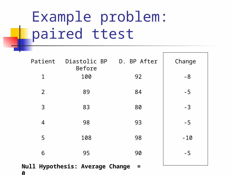
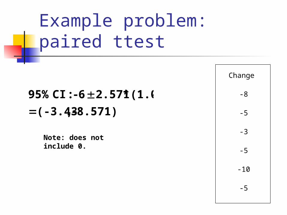
Example problem: paired ttest
Patient Diastolic BP Before D. BP After Change
1 100 92 -8
2 89 84 -5
3 83 80 -3
4 98 93 -5
5 108 98 -10
6 95 90 -5
Null Hypothesis: Average Change = 0
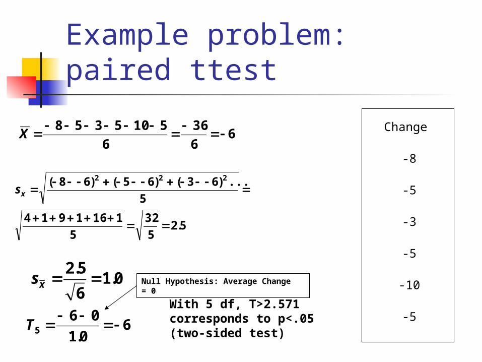
Example problem: paired ttest
Change
-8
-5
-3
-5
-10
-5
66
36
6
5105358
X
5.25
32
5
1161914
5
...)63()65()68( 222
xs
0.16
5.2xs
60.1
065
T
With 5 df, T>2.571 corresponds to p<.05 (two-sided test)
Null Hypothesis: Average Change = 0
Example problem: paired ttest
Change
-8
-5
-3
-5
-10
-5
8.571)- , (-3.43
(1.0)*2.5716- :CI 95%
Note: does not include 0.
Continuous outcome (means)
Outcome Variable
Are the observations correlated? Alternatives if the normality assumption is violated (and small n):
independent correlated
Continuous(e.g. blood pressure, age, pain score)
Ttest: compares means between two independent groups
ANOVA: compares means between more than two independent groups
Pearson’s correlation coefficient (linear correlation): shows linear correlation between two continuous variables
Linear regression: multivariate regression technique when the outcome is continuous; gives slopes or adjusted means
Paired ttest: compares means between two related groups (e.g., the same subjects before and after)
Repeated-measures ANOVA: compares changes over time in the means of two or more groups (repeated measurements)
Mixed models/GEE modeling: multivariate regression techniques to compare changes over time between two or more groups
Non-parametric statisticsWilcoxon sign-rank test: non-parametric alternative to paired ttest
Wilcoxon sum-rank test (=Mann-Whitney U test): non-parametric alternative to the ttest
Kruskal-Wallis test: non-parametric alternative to ANOVA
Spearman rank correlation coefficient: non-parametric alternative to Pearson’s correlation coefficient
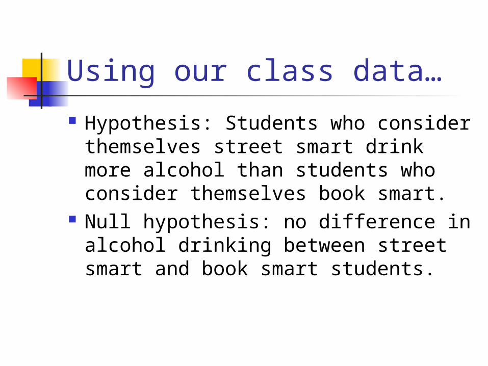
Using our class data…
Hypothesis: Students who consider themselves street smart drink more alcohol than students who consider themselves book smart.
Null hypothesis: no difference in alcohol drinking between street smart and book smart students.
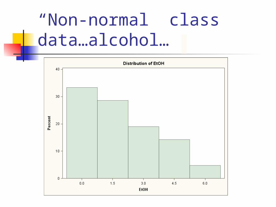
“Non-normal” class data…alcohol…
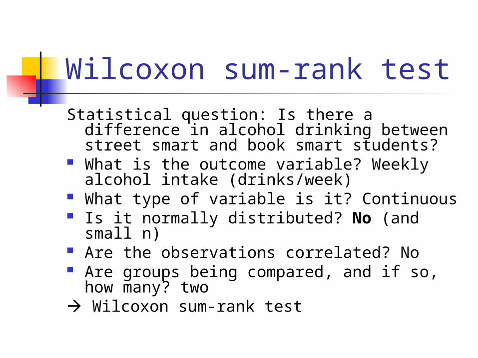
Wilcoxon sum-rank testStatistical question: Is there a difference in
alcohol drinking between street smart and book smart students?
What is the outcome variable? Weekly alcohol intake (drinks/week)
What type of variable is it? Continuous Is it normally distributed? No (and small n) Are the observations correlated? No Are groups being compared, and if so, how
many? two Wilcoxon sum-rank test
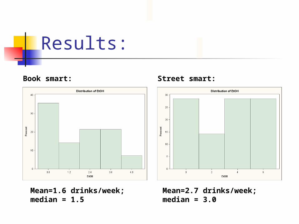
Results:
Mean=1.6 drinks/week; median = 1.5
Book smart: Street smart:
Mean=2.7 drinks/week; median = 3.0
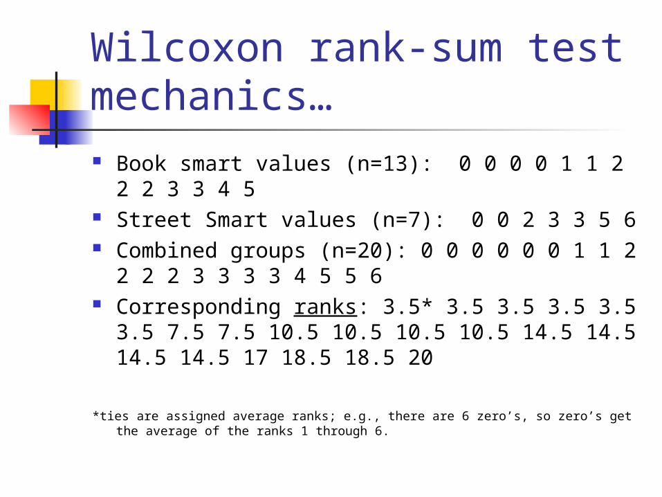
Wilcoxon rank-sum test mechanics… Book smart values (n=13): 0 0 0 0 1 1 2 2 2 3
3 4 5 Street Smart values (n=7): 0 0 2 3 3 5 6 Combined groups (n=20): 0 0 0 0 0 0 1 1 2 2 2
2 3 3 3 3 4 5 5 6 Corresponding ranks: 3.5* 3.5 3.5 3.5 3.5 3.5
7.5 7.5 10.5 10.5 10.5 10.5 14.5 14.5 14.5 14.5 17 18.5 18.5 20
*ties are assigned average ranks; e.g., there are 6 zero’s, so zero’s get the average of the ranks 1 through 6.
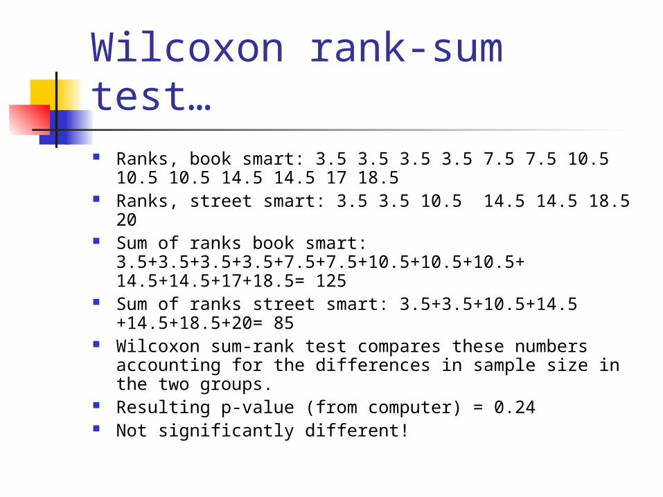
Wilcoxon rank-sum test… Ranks, book smart: 3.5 3.5 3.5 3.5 7.5 7.5 10.5 10.5
10.5 14.5 14.5 17 18.5 Ranks, street smart: 3.5 3.5 10.5 14.5 14.5 18.5 20 Sum of ranks book smart:
3.5+3.5+3.5+3.5+7.5+7.5+10.5+10.5+10.5+ 14.5+14.5+17+18.5= 125
Sum of ranks street smart: 3.5+3.5+10.5+14.5 +14.5+18.5+20= 85
Wilcoxon sum-rank test compares these numbers accounting for the differences in sample size in the two groups.
Resulting p-value (from computer) = 0.24 Not significantly different!
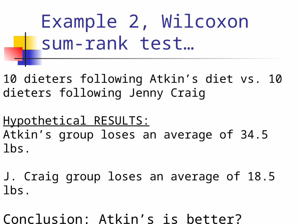
Example 2, Wilcoxon sum-rank test…
10 dieters following Atkin’s diet vs. 10 dieters following Jenny Craig
Hypothetical RESULTS:Atkin’s group loses an average of 34.5 lbs.
J. Craig group loses an average of 18.5 lbs.
Conclusion: Atkin’s is better?
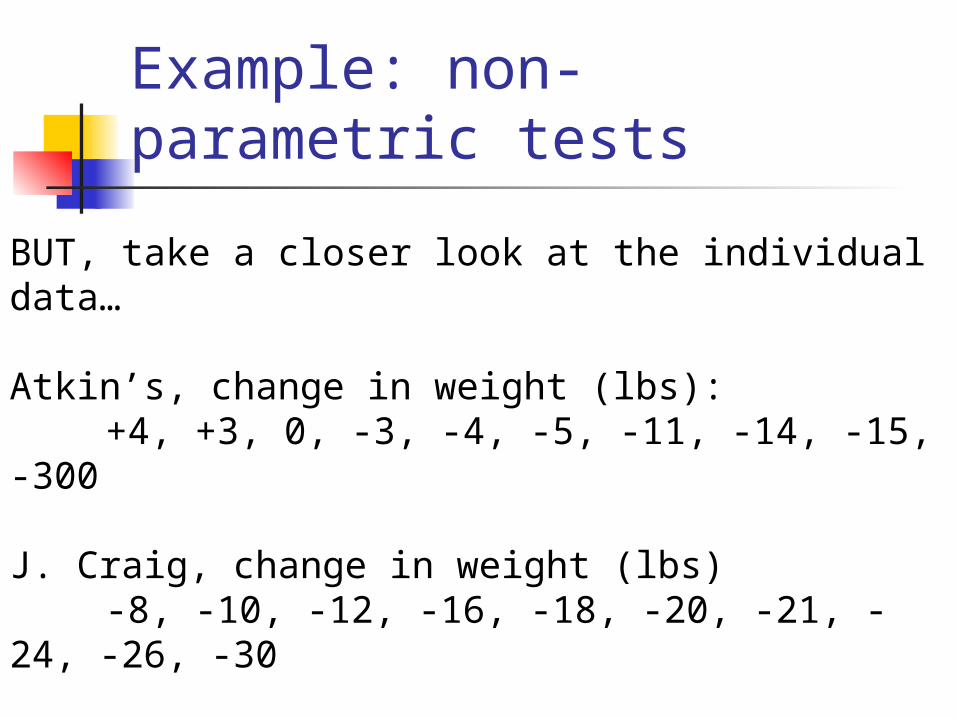
Example: non-parametric tests
BUT, take a closer look at the individual data…
Atkin’s, change in weight (lbs):+4, +3, 0, -3, -4, -5, -11, -14, -15, -300
J. Craig, change in weight (lbs)-8, -10, -12, -16, -18, -20, -21, -24, -26, -30
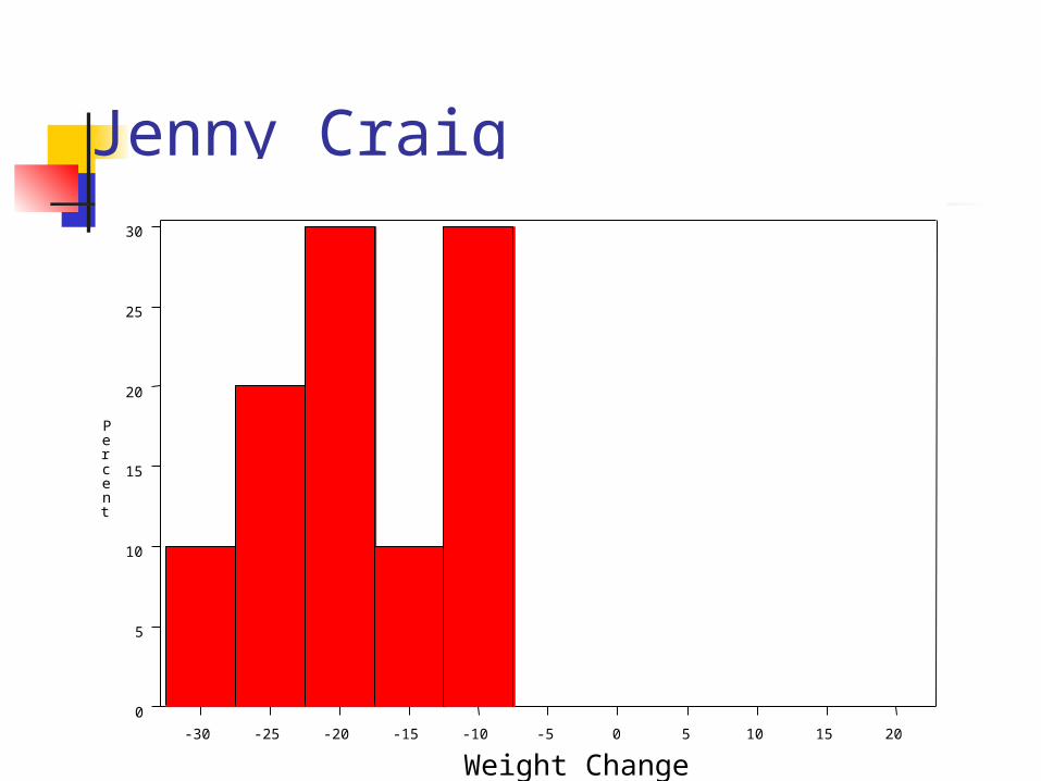
Jenny Craig
-30 -25 -20 -15 -10 -5 0 5 10 15 20
0
5
10
15
20
25
30
Percent
Weight Change
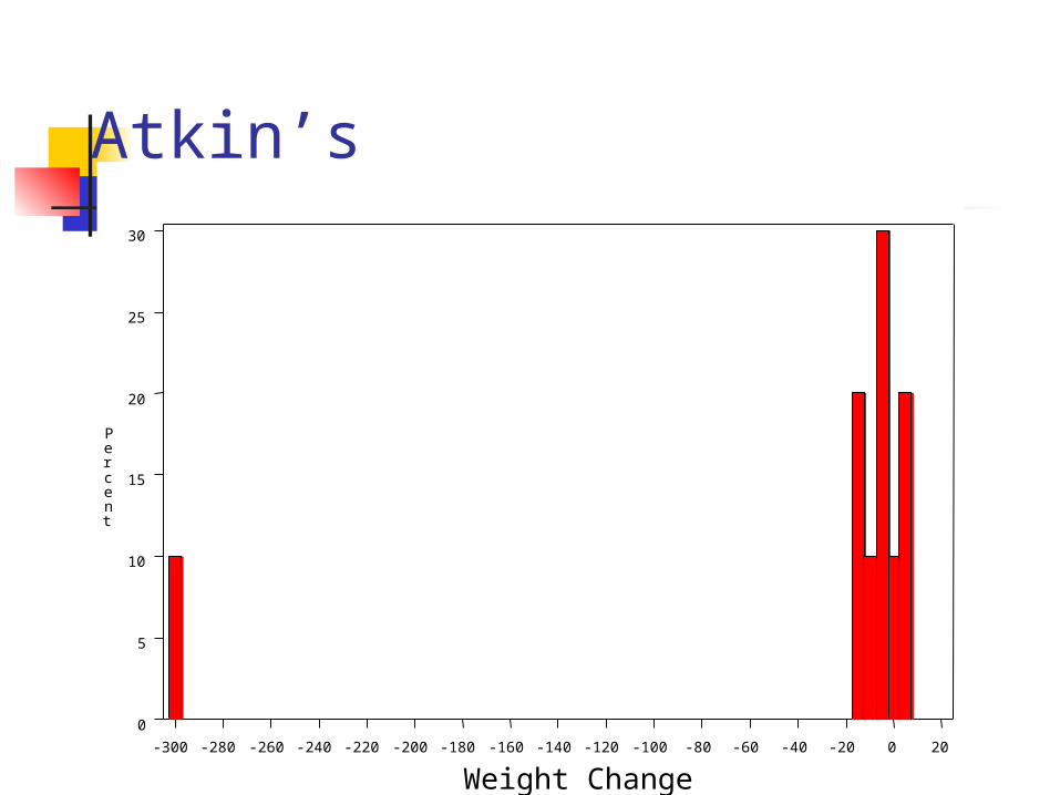
Atkin’s
-300 -280 -260 -240 -220 -200 -180 -160 -140 -120 -100 -80 -60 -40 -20 0 20
0
5
10
15
20
25
30
Percent
Weight Change
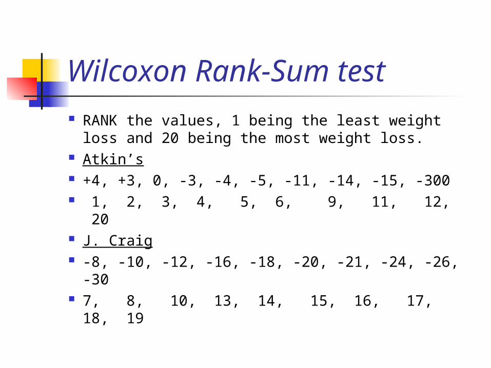
Wilcoxon Rank-Sum test RANK the values, 1 being the least weight
loss and 20 being the most weight loss. Atkin’s +4, +3, 0, -3, -4, -5, -11, -14, -15, -300 1, 2, 3, 4, 5, 6, 9, 11, 12, 20 J. Craig -8, -10, -12, -16, -18, -20, -21, -24, -26, -30 7, 8, 10, 13, 14, 15, 16, 17, 18, 19
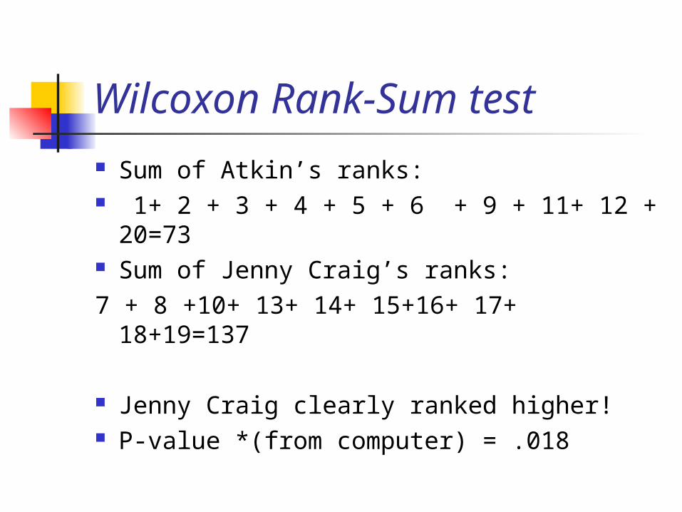
Wilcoxon Rank-Sum test Sum of Atkin’s ranks: 1+ 2 + 3 + 4 + 5 + 6 + 9 + 11+ 12 +
20=73 Sum of Jenny Craig’s ranks:7 + 8 +10+ 13+ 14+ 15+16+ 17+
18+19=137
Jenny Craig clearly ranked higher! P-value *(from computer) = .018
Review Question 3
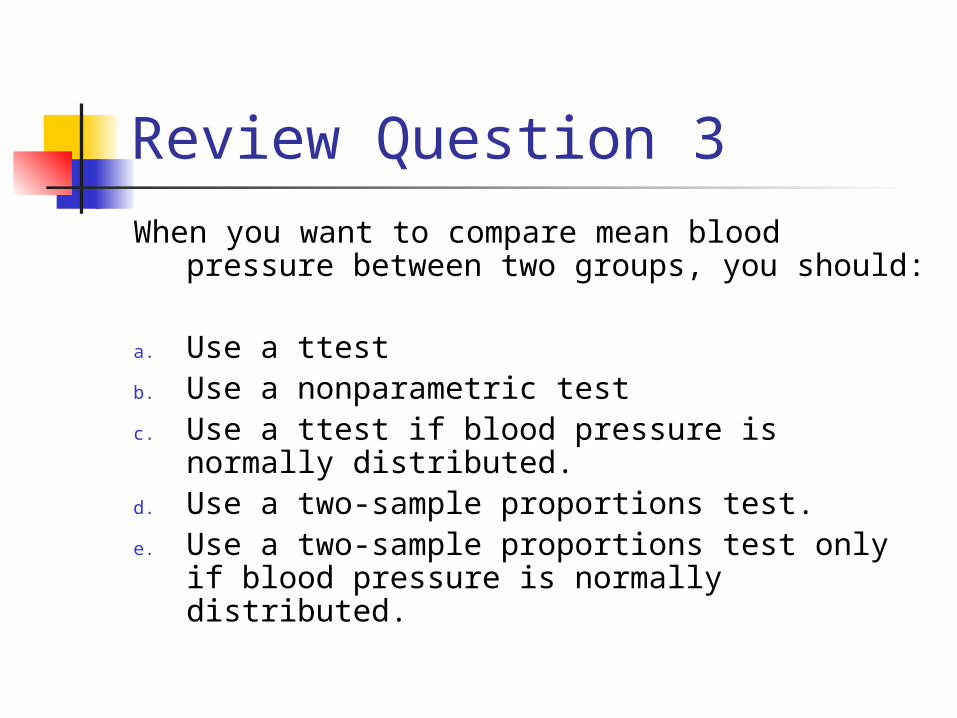
When you want to compare mean blood pressure between two groups, you should:
a. Use a ttestb. Use a nonparametric testc. Use a ttest if blood pressure is normally
distributed.d. Use a two-sample proportions test.e. Use a two-sample proportions test only if
blood pressure is normally distributed.
Review Question 3
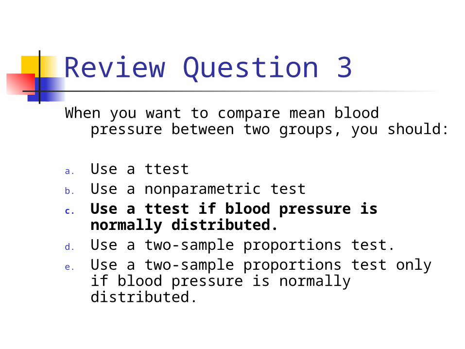
When you want to compare mean blood pressure between two groups, you should:
a. Use a ttestb. Use a nonparametric testc. Use a ttest if blood pressure is
normally distributed.d. Use a two-sample proportions test.e. Use a two-sample proportions test only if
blood pressure is normally distributed.

Continuous outcome (means)
Outcome Variable
Are the observations correlated? Alternatives if the normality assumption is violated (and small n):
independent correlated
Continuous(e.g. blood pressure, age, pain score)
Ttest: compares means between two independent groups
ANOVA: compares means between more than two independent groups
Pearson’s correlation coefficient (linear correlation): shows linear correlation between two continuous variables
Linear regression: multivariate regression technique when the outcome is continuous; gives slopes or adjusted means
Paired ttest: compares means between two related groups (e.g., the same subjects before and after)
Repeated-measures ANOVA: compares changes over time in the means of two or more groups (repeated measurements)
Mixed models/GEE modeling: multivariate regression techniques to compare changes over time between two or more groups
Non-parametric statisticsWilcoxon sign-rank test: non-parametric alternative to paired ttest
Wilcoxon sum-rank test (=Mann-Whitney U test): non-parametric alternative to the ttest
Kruskal-Wallis test: non-parametric alternative to ANOVA
Spearman rank correlation coefficient: non-parametric alternative to Pearson’s correlation coefficient
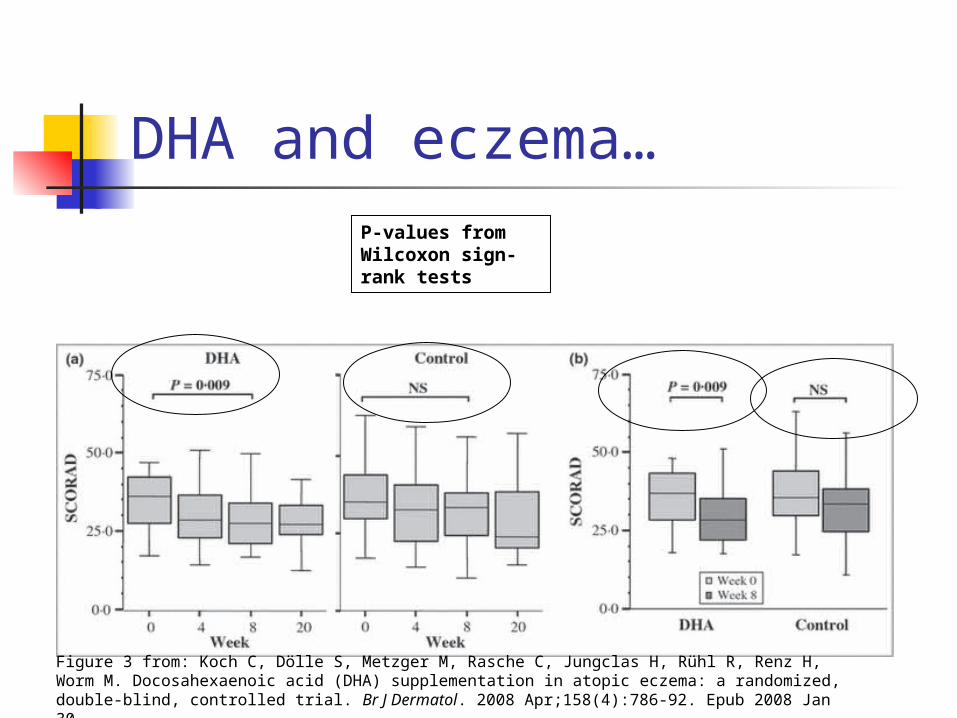
DHA and eczema…
Figure 3 from: Koch C, Dölle S, Metzger M, Rasche C, Jungclas H, Rühl R, Renz H, Worm M. Docosahexaenoic acid (DHA) supplementation in atopic eczema: a randomized, double-blind, controlled trial. Br J Dermatol. 2008 Apr;158(4):786-92. Epub 2008 Jan 30.
P-values from Wilcoxon sign-rank tests
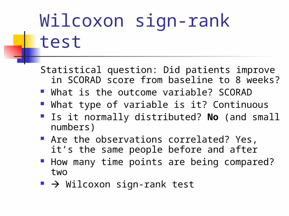
Wilcoxon sign-rank testStatistical question: Did patients improve in
SCORAD score from baseline to 8 weeks? What is the outcome variable? SCORAD What type of variable is it? Continuous Is it normally distributed? No (and small
numbers) Are the observations correlated? Yes, it’s the
same people before and after How many time points are being compared?
two Wilcoxon sign-rank test
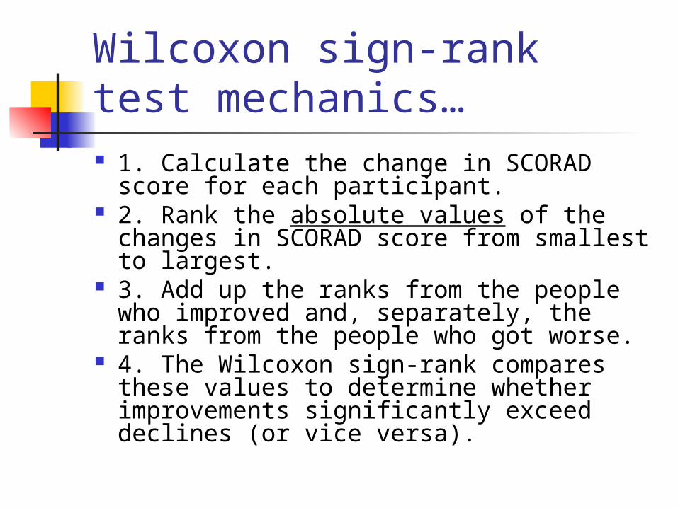
Wilcoxon sign-rank test mechanics… 1. Calculate the change in SCORAD score
for each participant. 2. Rank the absolute values of the
changes in SCORAD score from smallest to largest.
3. Add up the ranks from the people who improved and, separately, the ranks from the people who got worse.
4. The Wilcoxon sign-rank compares these values to determine whether improvements significantly exceed declines (or vice versa).

Continuous outcome (means)
Outcome Variable
Are the observations correlated? Alternatives if the normality assumption is violated (and small n):
independent correlated
Continuous(e.g. blood pressure, age, pain score)
Ttest: compares means between two independent groups
ANOVA: compares means between more than two independent groups
Pearson’s correlation coefficient (linear correlation): shows linear correlation between two continuous variables
Linear regression: multivariate regression technique when the outcome is continuous; gives slopes or adjusted means
Paired ttest: compares means between two related groups (e.g., the same subjects before and after)
Repeated-measures ANOVA: compares changes over time in the means of two or more groups (repeated measurements)
Mixed models/GEE modeling: multivariate regression techniques to compare changes over time between two or more groups
Non-parametric statisticsWilcoxon sign-rank test: non-parametric alternative to paired ttest
Wilcoxon sum-rank test (=Mann-Whitney U test): non-parametric alternative to the ttest
Kruskal-Wallis test: non-parametric alternative to ANOVA
Spearman rank correlation coefficient: non-parametric alternative to Pearson’s correlation coefficient
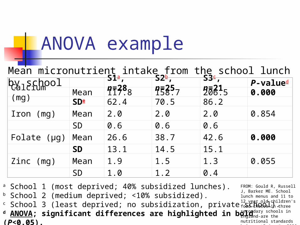
ANOVA example
S1a, n=28 S2b, n=25 S3c, n=21 P-valued
Calcium (mg) Mean 117.8 158.7 206.5 0.000SDe 62.4 70.5 86.2
Iron (mg) Mean 2.0 2.0 2.0 0.854
SD 0.6 0.6 0.6
Folate (μg) Mean 26.6 38.7 42.6 0.000
SD 13.1 14.5 15.1
Zinc (mg) Mean 1.9 1.5 1.3 0.055
SD 1.0 1.2 0.4a School 1 (most deprived; 40% subsidized lunches).b School 2 (medium deprived; <10% subsidized).c School 3 (least deprived; no subsidization, private school).d ANOVA; significant differences are highlighted in bold (P<0.05).
Mean micronutrient intake from the school lunch by school
FROM: Gould R, Russell J, Barker ME. School lunch menus and 11 to 12 year old children's food choice in three secondary schools in England-are the nutritional standards being met? Appetite. 2006 Jan;46(1):86-92.
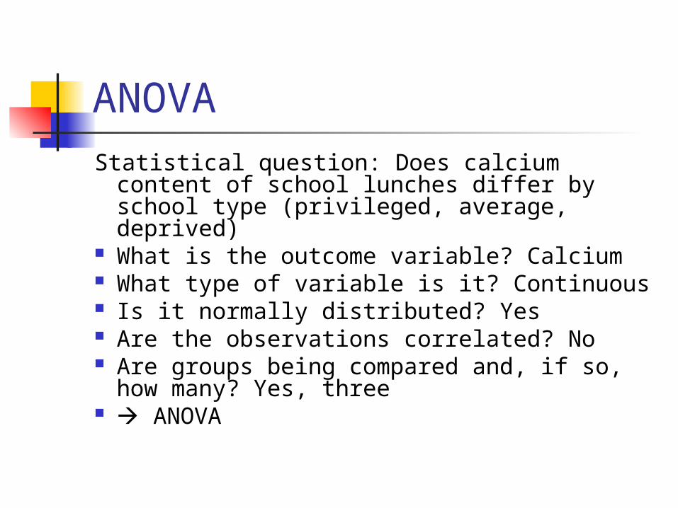
ANOVA
Statistical question: Does calcium content of school lunches differ by school type (privileged, average, deprived)
What is the outcome variable? Calcium What type of variable is it? Continuous Is it normally distributed? Yes Are the observations correlated? No Are groups being compared and, if so,
how many? Yes, three ANOVA
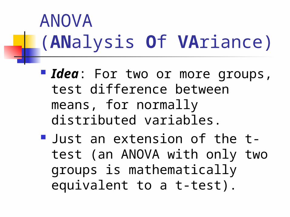
ANOVA (ANalysis Of VAriance)
Idea: For two or more groups, test difference between means, for normally distributed variables.
Just an extension of the t-test (an ANOVA with only two groups is mathematically equivalent to a t-test).
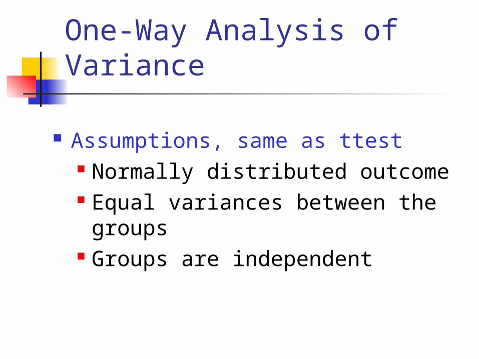
One-Way Analysis of Variance
Assumptions, same as ttest Normally distributed outcome Equal variances between the
groups Groups are independent
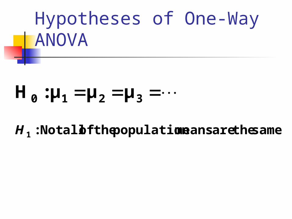
Hypotheses of One-Way ANOVA
3210 μμμ:H
same the are means population the of allNot :1H
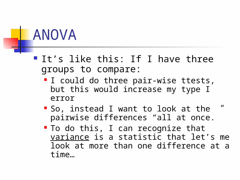
ANOVA It’s like this: If I have three groups
to compare: I could do three pair-wise ttests, but
this would increase my type I error So, instead I want to look at the
pairwise differences “all at once.” To do this, I can recognize that
variance is a statistic that let’s me look at more than one difference at a time…
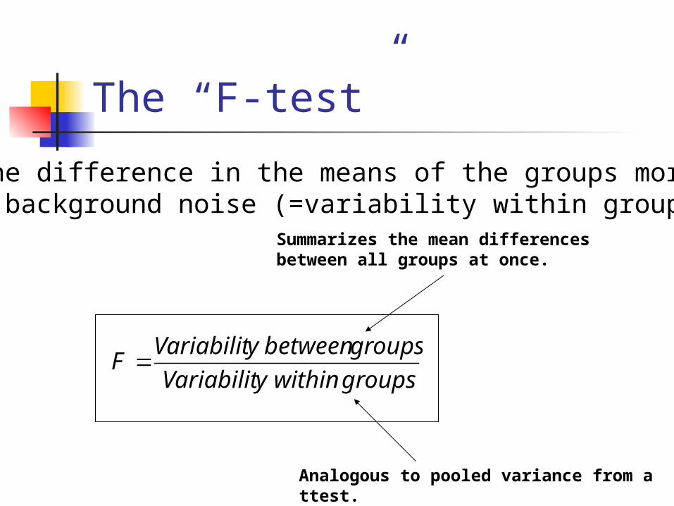
The “F-test”
groupswithinyVariabilit
groupsbetweenyVariabilitF
Is the difference in the means of the groups more than background noise (=variability within groups)?
Summarizes the mean differences between all groups at once.
Analogous to pooled variance from a ttest.
The F-distribution A ratio of variances follows an F-
distribution:
22
220
:
:
withinbetweena
withinbetween
H
H
The F-test tests the hypothesis that two variances are equal. F will be close to 1 if sample variances are equal.
mnwithin
between F ,2
2
~
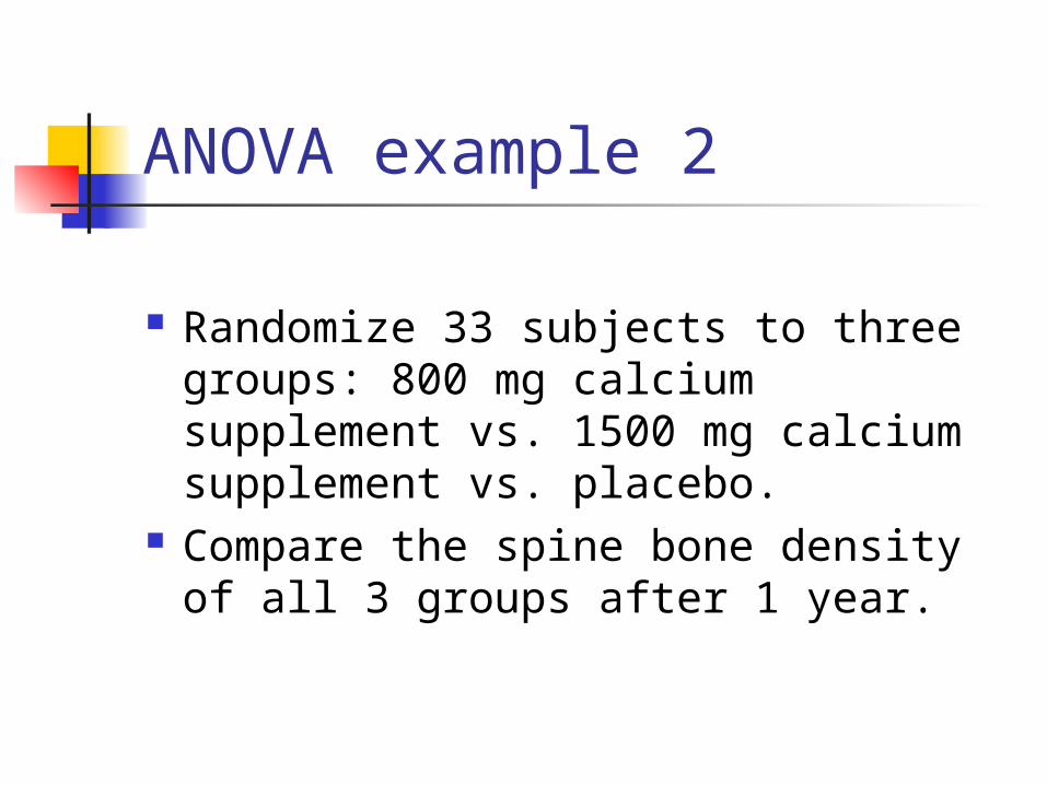
ANOVA example 2
Randomize 33 subjects to three groups: 800 mg calcium supplement vs. 1500 mg calcium supplement vs. placebo.
Compare the spine bone density of all 3 groups after 1 year.
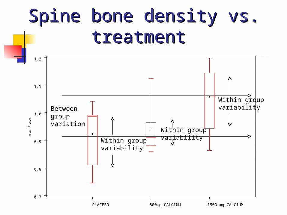
PLACEBO 800mg CALCIUM 1500 mg CALCIUM
0.7
0.8
0.9
1.0
1.1
1.2
SPINE
Between group variation
Spine bone density vs. Spine bone density vs. treatment treatment
Within group variability
Within group variability
Within group variability
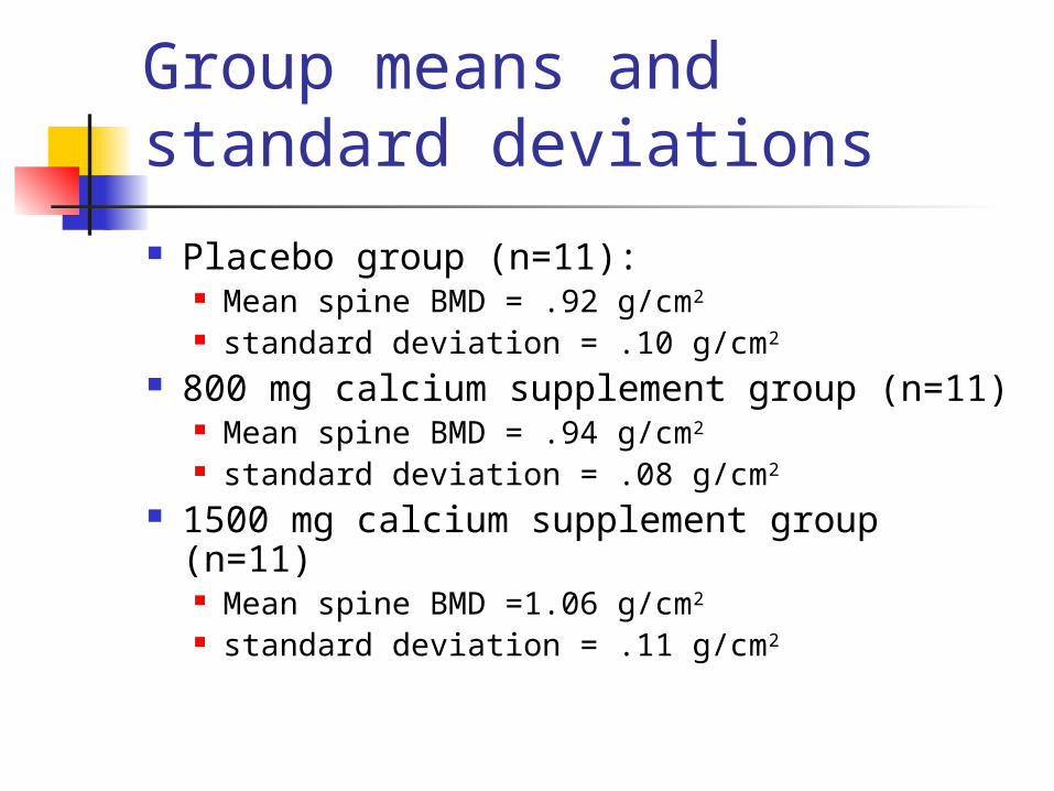
Group means and standard deviations
Placebo group (n=11): Mean spine BMD = .92 g/cm2
standard deviation = .10 g/cm2
800 mg calcium supplement group (n=11) Mean spine BMD = .94 g/cm2
standard deviation = .08 g/cm2
1500 mg calcium supplement group (n=11) Mean spine BMD =1.06 g/cm2
standard deviation = .11 g/cm2
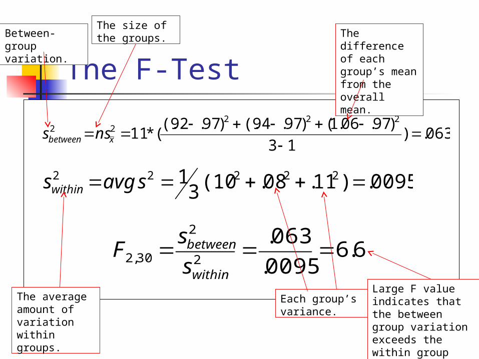
The F-Test
063.)13
)97.06.1()97.94(.)97.92(.(*11
22222
xbetween nss
0095.)11.08.10(.31 22222 savgswithin
6.60095.
063.2
2
30,2 within
between
s
sF
The size of the groups. The difference of
each group’s mean from the overall mean.
Between-group variation.
The average amount of variation within groups.
Each group’s variance.Large F value indicates that the between group variation exceeds the within group variation (=the background noise).
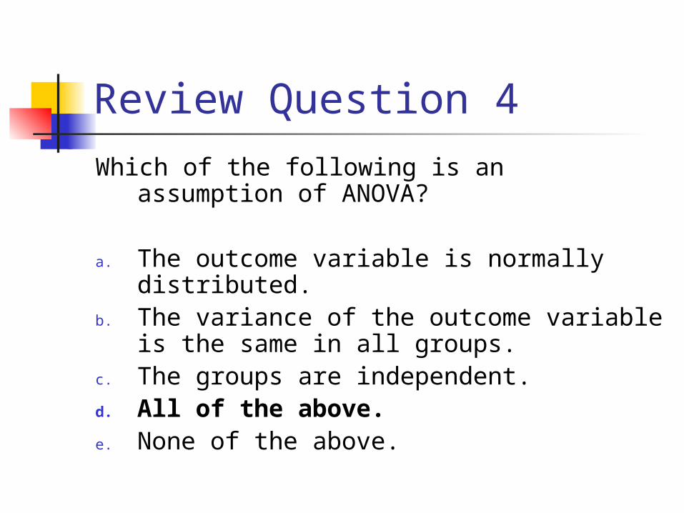
Review Question 4
Which of the following is an assumption of ANOVA?
a. The outcome variable is normally distributed.
b. The variance of the outcome variable is the same in all groups.
c. The groups are independent.d. All of the above.e. None of the above.
Review Question 4
Which of the following is an assumption of ANOVA?
a. The outcome variable is normally distributed.
b. The variance of the outcome variable is the same in all groups.
c. The groups are independent.d. All of the above.e. None of the above.
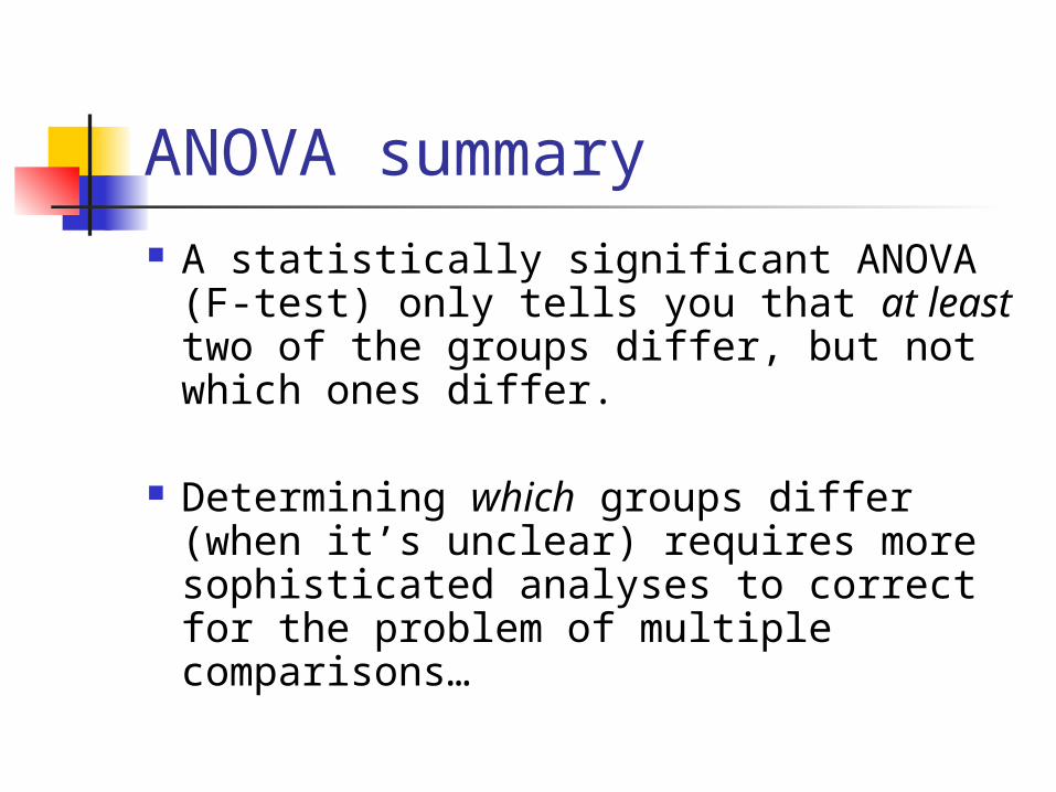
ANOVA summary A statistically significant ANOVA (F-
test) only tells you that at least two of the groups differ, but not which ones differ.
Determining which groups differ (when it’s unclear) requires more sophisticated analyses to correct for the problem of multiple comparisons…
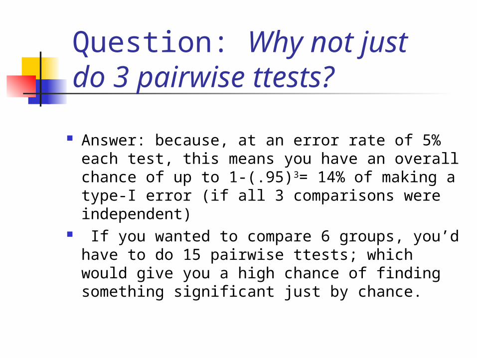
Question: Why not just do 3 pairwise ttests?
Answer: because, at an error rate of 5% each test, this means you have an overall chance of up to 1-(.95)3= 14% of making a type-I error (if all 3 comparisons were independent)
If you wanted to compare 6 groups, you’d have to do 15 pairwise ttests; which would give you a high chance of finding something significant just by chance.
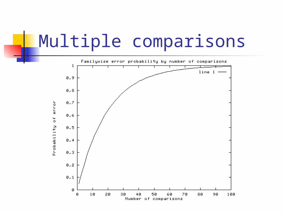
Multiple comparisons
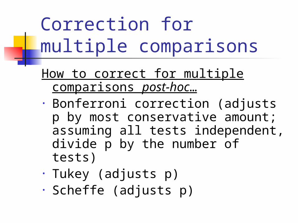
Correction for multiple comparisonsHow to correct for multiple
comparisons post-hoc…• Bonferroni correction (adjusts p by
most conservative amount; assuming all tests independent, divide p by the number of tests)
• Tukey (adjusts p)• Scheffe (adjusts p)
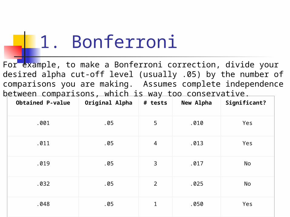
1. Bonferroni
Obtained P-value Original Alpha # tests New Alpha Significant?
.001 .05 5 .010 Yes
.011 .05 4 .013 Yes
.019 .05 3 .017 No
.032 .05 2 .025 No
.048 .05 1 .050 Yes
For example, to make a Bonferroni correction, divide your desired alpha cut-off level (usually .05) by the number of comparisons you are making. Assumes complete independence between comparisons, which is way too conservative.
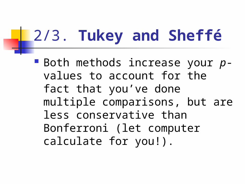
2/3. Tukey and Sheffé
Both methods increase your p-values to account for the fact that you’ve done multiple comparisons, but are less conservative than Bonferroni (let computer calculate for you!).
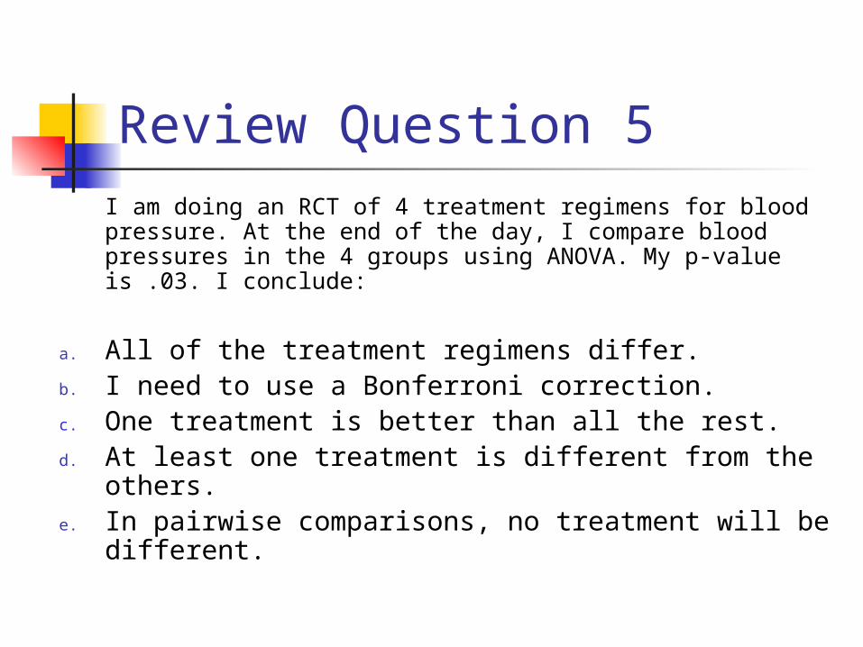
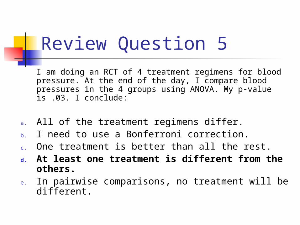
Review Question 5I am doing an RCT of 4 treatment regimens for blood pressure. At the end of the day, I compare blood pressures in the 4 groups using ANOVA. My p-value is .03. I conclude:
a. All of the treatment regimens differ.b. I need to use a Bonferroni correction.c. One treatment is better than all the rest.d. At least one treatment is different from the others. e. In pairwise comparisons, no treatment will be
different.
Review Question 5I am doing an RCT of 4 treatment regimens for blood pressure. At the end of the day, I compare blood pressures in the 4 groups using ANOVA. My p-value is .03. I conclude:
a. All of the treatment regimens differ.b. I need to use a Bonferroni correction.c. One treatment is better than all the rest.d. At least one treatment is different from the
others. e. In pairwise comparisons, no treatment will be
different.
Continuous outcome (means)
Outcome Variable
Are the observations correlated? Alternatives if the normality assumption is violated (and small n):
independent correlated
Continuous(e.g. blood pressure, age, pain score)
Ttest: compares means between two independent groups
ANOVA: compares means between more than two independent groups
Pearson’s correlation coefficient (linear correlation): shows linear correlation between two continuous variables
Linear regression: multivariate regression technique when the outcome is continuous; gives slopes or adjusted means
Paired ttest: compares means between two related groups (e.g., the same subjects before and after)
Repeated-measures ANOVA: compares changes over time in the means of two or more groups (repeated measurements)
Mixed models/GEE modeling: multivariate regression techniques to compare changes over time between two or more groups
Non-parametric statisticsWilcoxon sign-rank test: non-parametric alternative to paired ttest
Wilcoxon sum-rank test (=Mann-Whitney U test): non-parametric alternative to the ttest
Kruskal-Wallis test: non-parametric alternative to ANOVA
Spearman rank correlation coefficient: non-parametric alternative to Pearson’s correlation coefficient
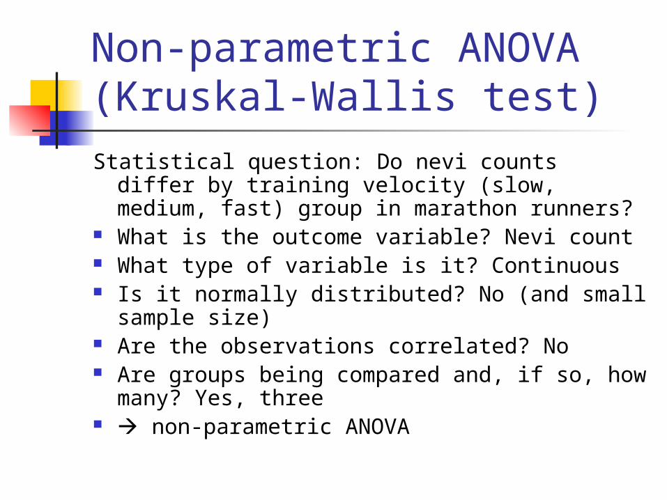
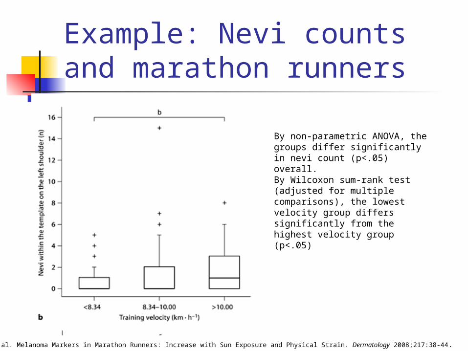
Non-parametric ANOVA (Kruskal-Wallis test)Statistical question: Do nevi counts differ by
training velocity (slow, medium, fast) group in marathon runners?
What is the outcome variable? Nevi count What type of variable is it? Continuous Is it normally distributed? No (and small
sample size) Are the observations correlated? No Are groups being compared and, if so, how
many? Yes, three non-parametric ANOVA
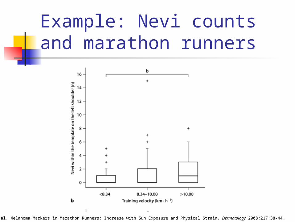
Example: Nevi counts and marathon runners
Richtig et al. Melanoma Markers in Marathon Runners: Increase with Sun Exposure and Physical Strain. Dermatology 2008;217:38-44.
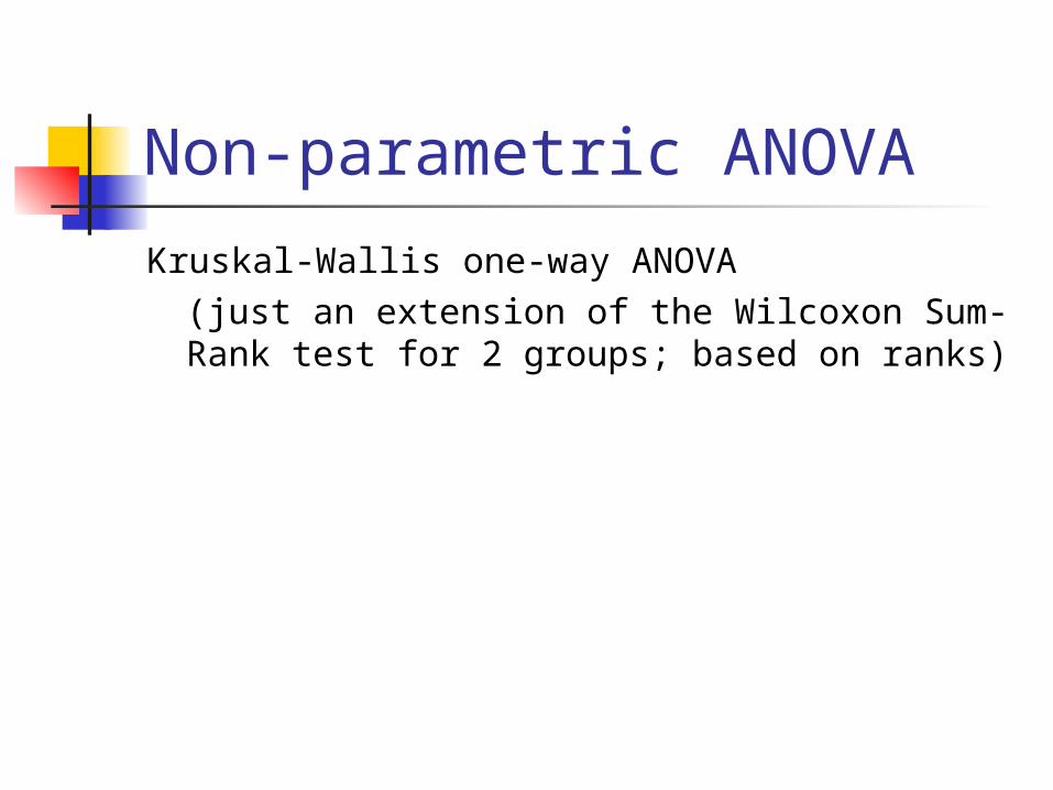
Non-parametric ANOVA
Kruskal-Wallis one-way ANOVA(just an extension of the Wilcoxon Sum-Rank test for 2 groups; based on ranks)
Example: Nevi counts and marathon runners
Richtig et al. Melanoma Markers in Marathon Runners: Increase with Sun Exposure and Physical Strain. Dermatology 2008;217:38-44.
By non-parametric ANOVA, the groups differ significantly in nevi count (p<.05) overall. By Wilcoxon sum-rank test (adjusted for multiple comparisons), the lowest velocity group differs significantly from the highest velocity group (p<.05)
Review Question 6I want to compare depression scores between three groups, but I’m not sure if depression is normally distributed. What should I do?
a. Don’t worry about it—run an ANOVA anyway.b. Test depression for normality.c. Use a Kruskal-Wallis (non-parametric) ANOVA. d. Nothing, I can’t do anything with these data.e. Run 3 nonparametric ttests.
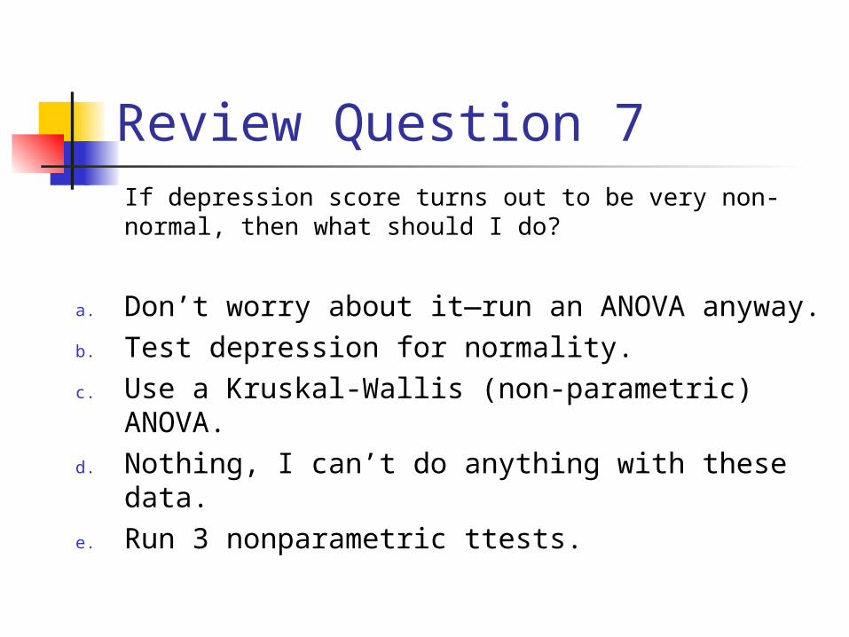
Review Question 7If depression score turns out to be very non-normal, then what should I do?
a. Don’t worry about it—run an ANOVA anyway.b. Test depression for normality.c. Use a Kruskal-Wallis (non-parametric) ANOVA. d. Nothing, I can’t do anything with these data.e. Run 3 nonparametric ttests.
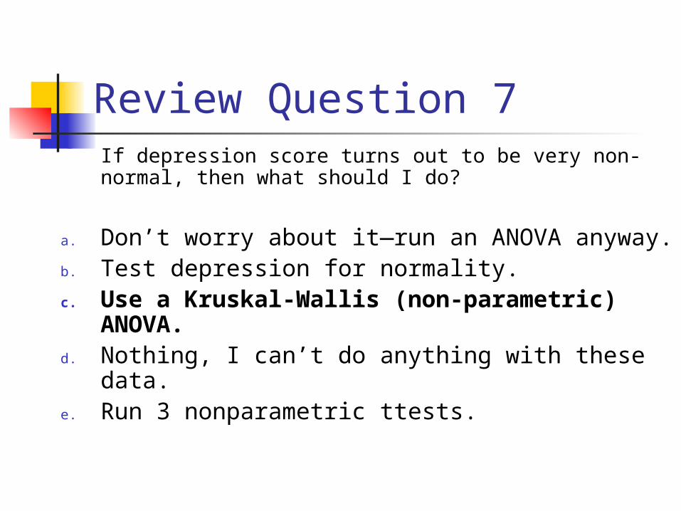
Review Question 7If depression score turns out to be very non-normal, then what should I do?
a. Don’t worry about it—run an ANOVA anyway.b. Test depression for normality.c. Use a Kruskal-Wallis (non-parametric)
ANOVA. d. Nothing, I can’t do anything with these data.e. Run 3 nonparametric ttests.
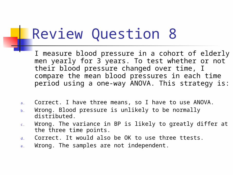
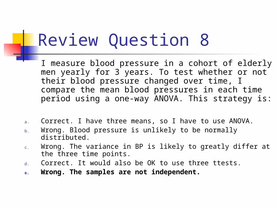
Review Question 8I measure blood pressure in a cohort of elderly men yearly for 3 years. To test whether or not their blood pressure changed over time, I compare the mean blood pressures in each time period using a one-way ANOVA. This strategy is:
a. Correct. I have three means, so I have to use ANOVA.b. Wrong. Blood pressure is unlikely to be normally distributed.c. Wrong. The variance in BP is likely to greatly differ at the
three time points.d. Correct. It would also be OK to use three ttests.e. Wrong. The samples are not independent.