introduction to deep learning - computer...
TRANSCRIPT

Introduction to Deep Learning
CS468 Spring 2017
Charles Qi

What is Deep Learning?
Deep learning allows computational models that are composed of multiple processing layers to learn representations of data with multiple levels of abstraction.
ArtificialIntelligence
MachineLearning
DeepLearning
Deep Learning by Y. LeCun et al. Nature 2015

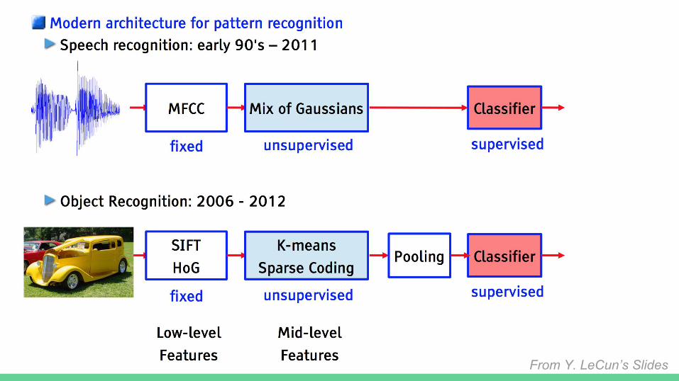
From Y. LeCun’s Slides

Image: HoG
Image: SIFT
Audio: Spectrogram
Point Cloud: PFH

From Y. LeCun’s Slides
Linear RegressionSVMDecision TreesRandom Forest...

Can we automatically learn “good” feature representations?
Image
Thermal Infrared
Video 3D CAD Model
Depth Scan Audio

From Y. LeCun’s Slides
From Y. LeCun’s Slides

From Y. LeCun’s Slides

From Y. LeCun’s Slides
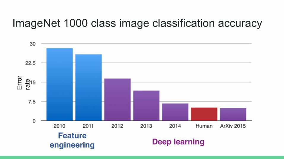
ImageNet 1000 class image classification accuracy

Big Data + Representation Learning with Deep Nets
Acoustic Modeling
Near human-level Text-To-Speech performance
By Google DeepMind
https://deepmind.com/blog/wavenet-generative-model-raw-audio/
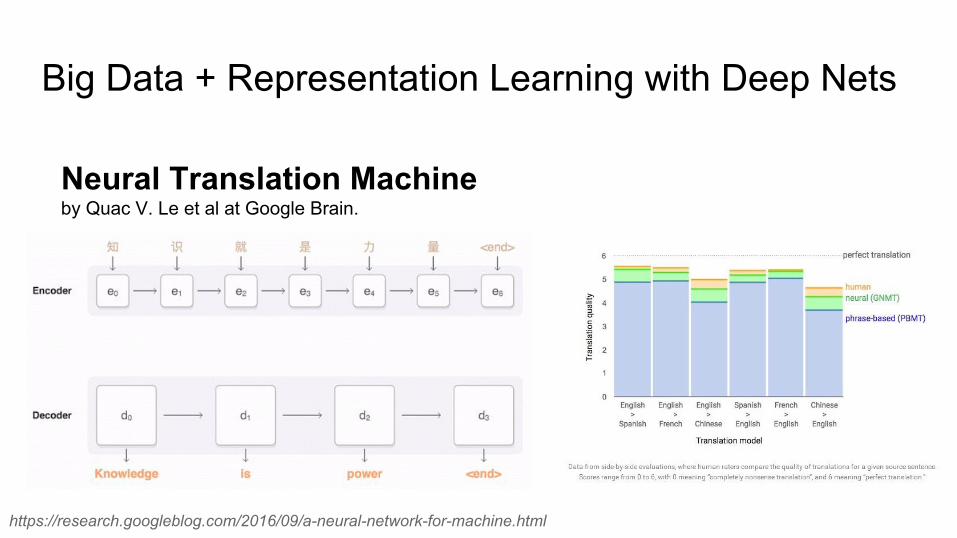
Big Data + Representation Learning with Deep Nets
Neural Translation Machine by Quac V. Le et al at Google Brain.
https://research.googleblog.com/2016/09/a-neural-network-for-machine.html

Outline
● Motivation● A Simple Neural Network● Ideas in Deep Net Architectures● Ideas in Deep Net Optimization● Practicals and Resources

Outline
● Motivation● A Simple Neural Network● Ideas in Deep Net Architectures● Ideas in Deep Net Optimization● Practicals and Resources
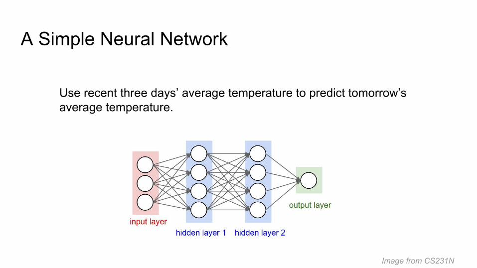
A Simple Neural Network
Image from CS231N
Use recent three days’ average temperature to predict tomorrow’s average temperature.

A Simple Neural Network
From CS231N
Sigmoid function
W1, b1, W2, b2, W3, b3are network parameters that need to be learned.
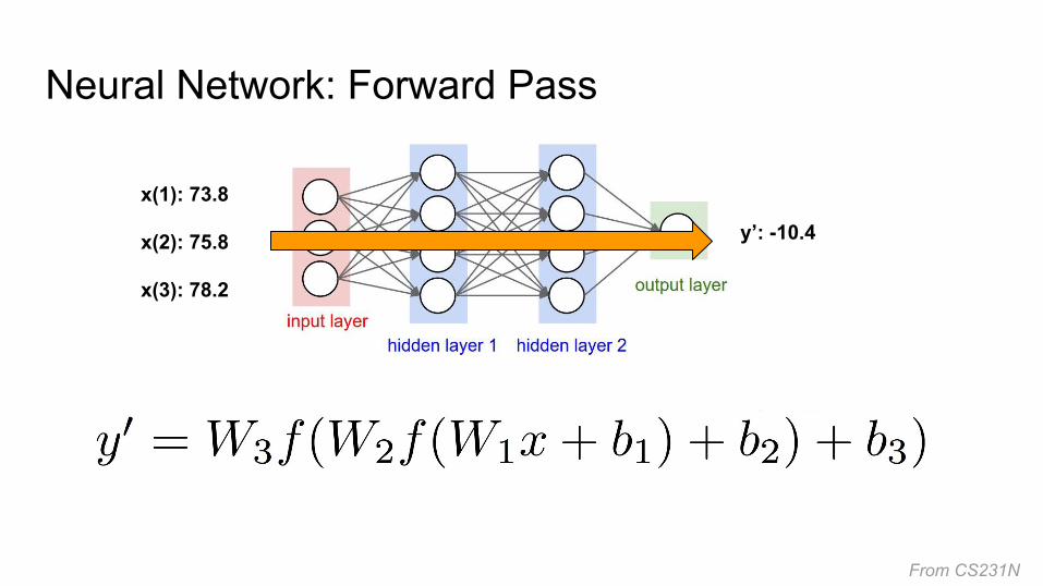
Neural Network: Forward Pass
From CS231N
x(1): 73.8
x(2): 75.8
x(3): 78.2
y’: -10.4

Neural Network: Backward Pass
73.8
75.8
78.2 Ground truth: 80.8
L2 error = (80.8 - (-10.4))^2
Update Network Parameters
Prediction: -10.4
Minimize:
Given N training pairs:

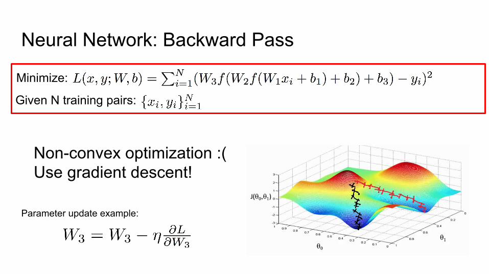
Neural Network: Backward Pass
Non-convex optimization :(
Minimize:
Given N training pairs:
Sigmoid function
Neural Network: Backward Pass
Non-convex optimization :(Use gradient descent!
Minimize:
Given N training pairs:
Parameter update example:

A Simple Neural Network
Model: Loss function:
Multi-Layer Perceptron (MLP)
L2 loss
Optimization: Gradient descent

Outline
● Motivation● A Simple Neural Network● Ideas in Deep Net Architectures● Ideas in Deep Net Optimization● Practicals and Resources

What people think I am doing when I “build a deep learning model”
What I actually do...
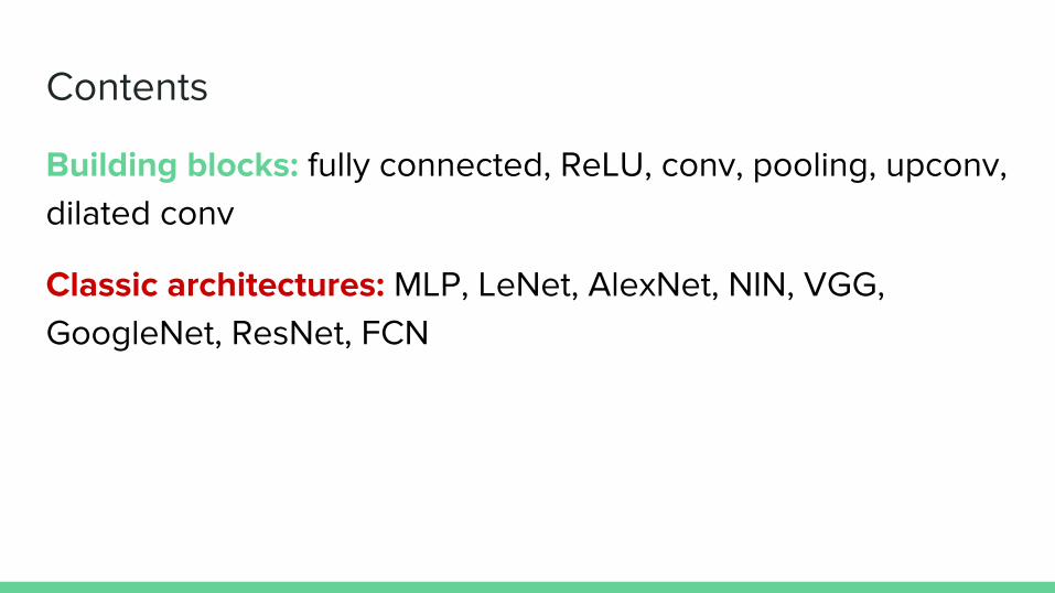
Contents
Building blocks: fully connected, ReLU, conv, pooling, upconv, dilated conv
Classic architectures: MLP, LeNet, AlexNet, NIN, VGG, GoogleNet, ResNet, FCN
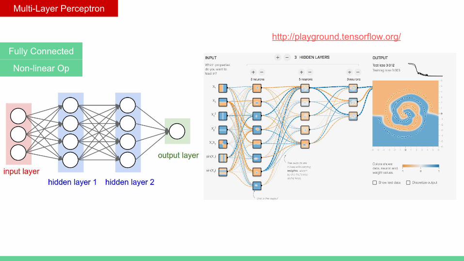
Multi-Layer Perceptron
http://playground.tensorflow.org/Fully Connected
Non-linear Op

Fully Connected
From LeCun’s Slides
● The first learning machine: the Perceptron Built at Cornell in 1960
● The Perceptron was a (binary) linear classifier on top of a simple feature extractor
From CS231N

Non-linear Op
Sigmoid
Tanh
From CS231N
Major drawbacks: Sigmoids saturate and kill gradients

Non-linear Op
ReLU (Rectified Linear Unit)
A plot from Krizhevsky et al. paper indicating the 6x improvement in convergence with the ReLU unit compared to the tanh unit.
Other Non-linear Op:
Leaky ReLU,
MaxOut From CS231N
+ Cheaper (linear) compared with Sigmoids (exp)+ No gradient saturation, faster in convergence- “Dead” neurons if learning rate set too high
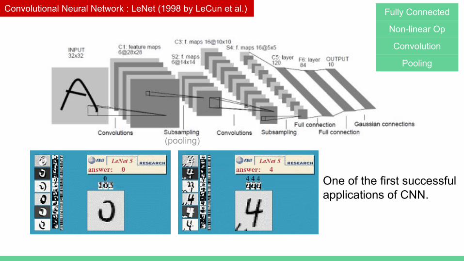
Convolutional Neural Network : LeNet (1998 by LeCun et al.) Fully Connected
Non-linear Op
Convolution
Pooling
One of the first successful applications of CNN.
(pooling)

Convolution
Slide from LeCun
Fully Connected NN in high dimension
Shared Weights & Convolutions:Exploiting Stationarity

Convolution
From CS231N
Stride 1 Stride 2
Pad 1Stride 2
From vdumoulin/conv_arithmetic
Pad 1Stride 1

Convolution
Pad 1Stride 2
5x5 RGB Image 5x5x3 array
3x3 kernel, 2 output channels, pad 1, stride 2
weights: 2x3x3x3 arraybias: 2x1 array
Output3x3x2 array
H’ = (H - K)/stride_H + 1= (7-3)/2 + 1 = 3
From CS231N

Pooling
Discarding pooling layers has been found to be important in training good generative models, such as variational autoencoders (VAEs) or generative adversarial networks (GANs).It seems likely that future architectures will feature very few to no pooling layers.
From CS231N
Pooling layer (usually inserted in between conv layers) is used to reduce spatial size of the input, thus reduce number of parameters and overfitting.

LeNet (1998 by LeCun et al.) Fully Connected
Non-linear Op
Convolution
Pooling
(pooling)

AlexNet (2012 by Krizhevsky et al.)
What’s different?
The first work that popularized Convolutional Networks in Computer Vision

AlexNet (2012 by Krizhevsky et al.)
What’s different?
● Big data: ImageNet● GPU implementation: more than 10x speedup● Algorithm improvement: deeper network, data
augmentation, ReLU, dropout, normalization layers etc.
Our network takes between five and six days to train on two GTX 580 3GB GPUs. -- Alex

Network in Network (2013 by Min Lin et al.)
56x56x128 256x5x5x128 weights 256x5x5x256 weights 256x5x5x256 weights
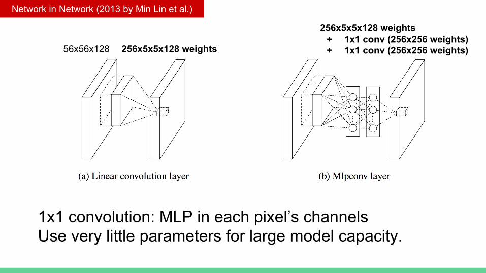
Network in Network (2013 by Min Lin et al.)
1x1 convolution: MLP in each pixel’s channelsUse very little parameters for large model capacity.
56x56x128 256x5x5x128 weights
256x5x5x128 weights+ 1x1 conv (256x256 weights)+ 1x1 conv (256x256 weights)

VGG (2014 by Simonyan and Zisserman)
Karen Simonyan, Andrew Zisserman: Very Deep Convolutional Networks for Large-Scale Image Recognition.
● Its main contribution was in showing that the depth of the network is a critical component for good performance.
● Their final best network contains 16 CONV/FC layers and, appealingly, features an extremely homogeneous architecture that only performs 3x3 convolutions and 2x2 pooling from the beginning to the end.
-- quoted from CS231N
The runner-up in ILSVRC 2014

GoogleNet (2015 by Szegedy et al.)
An Inception Module: a new building block..
Its main contribution was the development of an Inception Module and the using Average Pooling instead of Fully Connected layers at the top of the ConvNet, which dramatically reduced the number of parameters in the network (4M, compared to AlexNet with 60M).
-- edited from CS231N
Tip on ConvNets:Usually, most computation is spent on convolutions, while most space is spent on fully connected layers.
The winner in ILSVRC 2014

ResNet (2016 by Kaiming He et al.) The winner in ILSVRC 2015
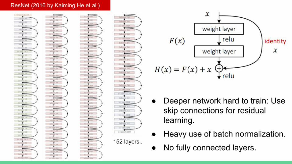
ResNet (2016 by Kaiming He et al.)
● Deeper network hard to train: Use skip connections for residual learning.
● Heavy use of batch normalization.
● No fully connected layers.152 layers..
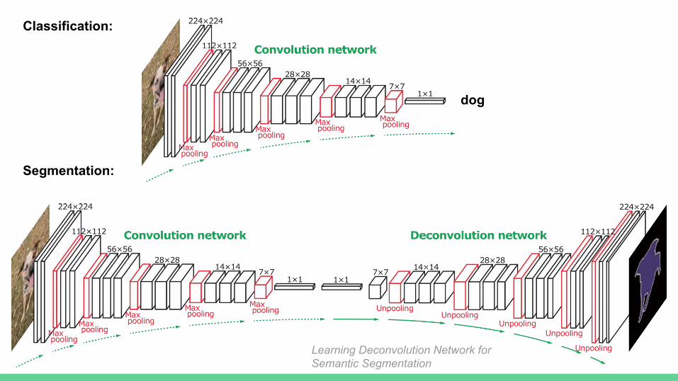
dog
Classification:
Segmentation:
Learning Deconvolution Network for Semantic Segmentation
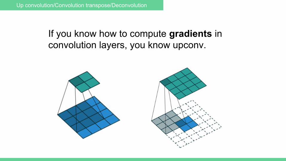
Up convolution/Convolution transpose/Deconvolution
If you know how to compute gradients in convolution layers, you know upconv.

Up convolution/Convolution transpose/Deconvolution
11 12 13 14
21 22 23 24
31 32 33 34
41 42 43 44
11 12
21 22
11 12 13
21 22 23
31 32 33
x w y

Up convolution/Convolution transpose/Deconvolution
11 12 13 14
21 22 23 24
31 32 33 34
41 42 43 44
11 12
21 22
11 12 13
21 22 23
31 32 33
x w y

Convolution with stride =>Upconvolution with input upsampling
Upconvolution/Convolution transpose/Deconvolution
See https://github.com/vdumoulin/conv_arithmetic for examples

Dilated Convolution
Fully convolutional network (FCN) variations
Input image HxWx3
dilated conv
Output scores HxWxN
conv
upconv
Input image HxWx3
Output scoresHxWxN
Skip links
Input image HxWx3
Output scoresHxWxN
conv
upsample

Dilated/Atrous Convolution
Issues with convolution in dense prediction (image segmentation)● Use small kernels
○ Receptive field grows linearly with #layers: l∗(k−1)+k● Use large kernels
○ loss of resolution
Dilated convolutions support exponentially expanding receptive fields without losing resolution or coverage.
Fig from ICLR 16 paper by Yu and Koltun.
L1: dilation=1 L2: dilation=2 L2: dilation=4
dilation=2
Receptive field: 3 Receptive field: 7 Receptive field: 15

Fig from ICLR 16 paper by Yu and Koltun.
Dilated/Atrous Convolution
Baseline: conv + FC Dilated conv
Outline
● Motivation● A Simple Neural Network● Ideas in Deep Net Architectures● Ideas in Deep Net Optimization● Practicals and Resources

Optimization
Basics: Gradient descent, SGD, mini-batch SGD, Momentum, Adam, learning rate decay
Other Ingredients: Data augmentation, Regularization, Dropout, Xavier initialization, Batch normalization

NN Optimization:Back Propagation [Hinton et al. 1985]Gradient Descent with Chain Rule Rebranded.
Fig from Deep Learning by LeCun, Bengio and Hinton. Nature 2015

SGD, Momentum, RMSProp, Adagrad, Adam
● Batch gradient descent (GD):○ Update weights once after looking at all the training data.
● Stochastic gradient descent (SGD):○ Update weights for each sample.
● Mini-batch SGD:○ Update weights after looking at every “mini batch” of data, say 128 samples.
Let x be the weight/parameters, dx be the gradient of x. In mini-batch, dx is the average within a batch.
SGD (the vanilla update)
From CS231Nwhere learning_rate is a hyperparameter - a fixed constant.

SGD, Momentum, RMSProp, Adagrad, Adam
Initializing the parameters with random numbers is equivalent to setting a particle with zero initial velocity at some location.
The optimization process can then be seen as equivalent to the process of simulating the parameter vector (i.e. a particle) as rolling on the landscape.
Momentum:
From CS231N

SGD, Momentum, RMSProp, Adagrad, Adam
Adagrad by Duchi et al.:
Per-parameter adaptive learning rate methods
weights with high gradients => effective learning rate reduced
RMSProp by Hinton:Use moving average to reduce Adagrad’s aggressive, monotonically decreasing learning rate
Adam by Kingma et al.:
Use smoothed version of gradients compared with RMSProp. Default optimizer (along with Momentum).
From CS231N

Annealing the learning rate (the dark art...)
From Martin Gorner

Annealing the learning rate (the dark art...)
From Martin Gorner

Annealing the learning rate (the dark art...)
● Stairstep decay: Reduce the learning rate by some factor every few epochs. E.g. half the learning rate every 10 epochs.
● Exponential decay: learning_rate = initial_lr * exp(-kt) where t is current step.
● “On-demand” decay: Reduce the learning rate when error plateaus

Optimization
Basics: Gradient descent, SGD, mini-batch SGD, Momentum, Adam, learning rate decay
Other Ingredients: Data augmentation, Regularization, Dropout, Xavier initialization, Batch normalization

Dealing with Overfitting: Data Augmentation
Flipping, random crop, random translation, color/brightness change, adding noise...
Pictures from CS231N
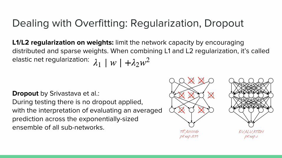
Dealing with Overfitting: Regularization, Dropout
L1/L2 regularization on weights: limit the network capacity by encouraging distributed and sparse weights. When combining L1 and L2 regularization, it’s called elastic net regularization:
Dropout by Srivastava et al.: During testing there is no dropout applied, with the interpretation of evaluating an averaged prediction across the exponentially-sized ensemble of all sub-networks.

Applying dropoutduring training

Xavier and MSR Initialization
Problem with random Gaussian initialization: the distribution of the outputs has a variance that grows with the number of inputs => Exploding/diminishing output in very deep network.
W = 0.01* np.random.randn(D,H)
w = np.random.randn(n) / sqrt(n).
w = np.random.randn(n) * sqrt(2/n).

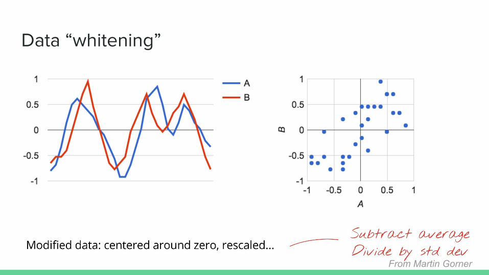
Data “whitening”
From Martin Gorner
Data “whitening”
From Martin Gorner

Batch Normalization
From Martin Gorner

Batch Normalization
From Martin Gorner
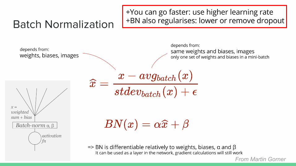
Batch Normalization
From Martin Gorner

Outline
● Motivation● A Simple Neural Network● Ideas in Deep Net Architectures● Ideas in Deep Net Optimization● Practicals and Resources
Image from Martin Gorner

Data Collecting, Cleaning, Preprocessing > 50% time
“OS” of Machine/Deep LearningCaffe, Theano, Torch, Tensorflow, Pytorch, MXNET, …Matlab in the earlier days. Python and C++ is the popular
choice now.
Deep network debugging, Visualizations
Resources
Stanford CS231N: Convolutional Neural Networks for Visual Recognition
Stanford CS224N: Natural Language Processing with Deep Learning
Berkeley CS294: Deep Reinforcement Learning
Learning Tensorflow and deep learning, without a PhD
Udacity and Coursera classes on Deep Learning
Book by Goodfellow, Bengio and Courville: http://www.deeplearningbook.org/
Talk by LeCun 2013: http://www.cs.nyu.edu/~yann/talks/lecun-ranzato-icml2013.pdf
Talk by Hinton, Bengio, LeCun 2015: https://www.iro.umontreal.ca/~bengioy/talks/DL-Tutorial-NIPS2015.pdf

What’s not covered...
Sequential Models (RNN, LSTM, GRU)
Deep Reinforcement Learning
3D Deep Learning (MVCNN, 3D CNN, Spectral CNN, NN on Point Sets)
Generative and Unsupervised Models (AE, VAE, GAN etc.)
Theories in Deep Learning
...

Summary
● Why Deep Learning
● A Simple Neural Network○ Model, Loss and Optimization
● Ideas in deep net architectures○ Building blocks: FC, ReLU, conv, pooling, unpooling, upconv, dilated conv○ Classics: MLP, LeNet, AlexNet, NIN, VGG, GoogleNet, ResNet
● Ideas in deep net optimization○ Basics: GD, SGD, mini-batch SGD, Momentum, Adam, learning rate decay○ Other Ingredients: Data augmentation, Regularization, Dropout, Batch
normalization
● Practicals and Resources