Introduction to Differential Geometry & General Relativity

6th Printing May 2014

Lecture Notes by

Stefan Waner

with a Special Guest Lecture by Gregory C. Levine

Departments of Mathematics and Physics, Hofstra University

2

Introduction to Differential Geometry and General Relativity

Lecture Notes by Stefan Waner, with a Special Guest Lecture by Gregory C. Levine

Department of Mathematics, Hofstra University

These notes are dedicated to the memory of Hanno Rund.

TABLE OF CONTENTS 1. Preliminaries ......................................................................................................3 2. Smooth Manifolds and Scalar Fields ................................................................8 3. Tangent Vectors and the Tangent Space .......................................................16 4. Contravariant and Covariant Vector Fields .................................................26 5. Tensor Fields ....................................................................................................37 6. Riemannian Manifolds ....................................................................................42 7. Locally Minkowskian Manifolds: An Introduction to Relativity ................52 8. Covariant Differentiation ................................................................................63 9. Geodesics and Local Inertial Frames .............................................................71 10. The Riemann Curvature Tensor ..................................................................83 11. A Little More Relativity: Comoving Frames and Proper Time ................94 12. The Stress Tensor and the Relativistic Stress-Energy Tensor .................100 13. Two Basic Premises of General Relativity .................................................109 14. The Einstein Field Equations and Derivation of Newton's Law .............114 15. The Schwarzschild Metric and Event Horizons ........................................124 16. White Dwarfs, Neutron Stars and Black Holes, by Gregory C. Levine .131 References and Further Reading ................................................................138 The author is grateful to Daniel Metz (an appreciative reader) for his corrections that appear in the latest version, and to many of my students who uncovered errors and inconsistencies in previous versions.

3

1. Preliminaries Distance and Open Sets Here, we do just enough topology so as to be able to talk about smooth manifolds. We begin with n-dimensional Euclidean space En = {(y1, y2, . . . , yn) | yi é R}. Thus, E1 is just the real line, E2 is the Euclidean plane, and E3 is 3-dimensional Euclidean space. The magnitude, or norm, ||y || of y = (y1, y2, . . . , yn) in En is defined to be ||y || = y1

2 + y22 + . . . + yn

2 , which we think of as its distance from the origin. Thus, the distance between two points y = (y1, y2, . . . , yn) and z = (z1, z2, . . . , zn) in En is defined as the norm of z - y: Distance Formula Distance between y and z = ||z - y|| = (z1 - y1)

2 + (z2 - y2)2 + . . . + (zn - yn)

2 . Proposition 1.1 (Properties of the norm) The norm satisfies the following: (a) ||y || ≥ 0, and ||y || = 0 iff y = 0 (positive definite) (b) ||¬y|| = |¬|||y || for every ¬ é R and y é En. (c) ||y + z|| ≤ ||y || + ||z || for every y , z é En (triangle inequality 1) (d) ||y - z|| ≤ ||y - w|| + ||w - z|| for every y, z, w é En (triangle inequality 2) The proof of Proposition 1.1 is an exercise which may require reference to a linear algebra text (see “inner products”). Definition 1.2 A Subset U of En is called open if, for every y in U, all points of En within some positive distance r of y are also in U. (The size of r may depend on the point y chosen. Illustration in class). Intuitively, an open set is a solid region minus its boundary. If we include the boundary, we get a closed set, which formally is defined as the complement of an open set. Examples 1.3 (a) If a é En, then the open ball with center a and radius r is the subset B(a, r) = {x é En | ||x-a|| < r}.

4

Open balls are open sets: If x é B(a, r), then, with s = r - ||x-a||, one has B(x, s) ¯ˉ B(a, r). (b) En is open. (c) Ø is open. (d) Unions of open sets are open. (e) Open sets are unions of open balls. (Proof in class) Definition 1.4 Now let M ¯ˉ Es. A subset V ¯ˉ M is called open in M (or relatively open) if, for every y in V, all points of M within some positive distance r of y are also in V. Examples 1.5 (a) Open balls in M If M ¯ˉ Es, m é M, and r > 0, define BM(m, r) = {x é M | ||x-m|| < r}. Then BM(m, r) = B(m, r) Ú M, and so BM(m, r) is open in M. (b) M is open in M. (c) Ø is open in M. (d) Unions of open sets in M are open in M. (e) Open sets in M are unions of open balls in M. Parametric Paths and Surfaces in E3 and in Es From now on, the three coordinates of s-space will be referred to as y1, y2, ... , ys. Definition 1.6 A smooth path in E3 is a set of three smooth (infinitely differentiable) real-valued functions of a single real variable t: y1 = y1(t), y2 = y2(t), y3 = y3(t). The variable t is called the parameter of the curve. The path is non-singular if the

vector (dy1dt ,

dy2dt ,

dy3dt ) is nowhere zero.

Notes (a) Instead of writing y1 = y1(t), y2 = y2(t), y3 = y3(t), we shall simply write yi = yi(t).

5

(b) Since there is nothing special about three dimensions, we define a smooth path in En in exactly the same way: as a collection of smooth functions yi = yi(t), where this time i goes from 1 to n. Examples 1.7 (a) Straight lines in E3 (b) Curves in E3 (circles, etc.) Definition 1.8 A smooth surface embedded in E3 is a collection of three smooth real-valued functions of two variables x1 and x2 (notice that x finally makes a debut). y1 = y1(x

1, x2) y2 = y2(x

1, x2) y3 = y3(x

1, x2), or just yi = yi(x

1, x2) (i = 1, 2, 3). with domain some open set D in E2.

We also require that:

(a) The 3¿2 matrix whose ij entry is ∂yi

∂xj has rank two. (This is a local property which

says that the functions yi define an immersion.) (b) The associated function D→E3 is a one-to-one map (that is, distinct points (x1, x2)

in “parameter space” E2 give different points (y1, y2, y3) in E3). (This is a global property which says that the functions yi define an enbedding.)

We call x1 and x2 the parameters or local coordinates. Examples 1.9 (a) Planes in E3 and in Es (b) The paraboloid y3 = y1

2 + y22

(c) The sphere y12 + y2

2 + y32 = 1, using spherical polar coordinates:

y1 = sin x1 cos x2 y2 = sin x1 sin x2 y3 = cos x1

where 0 < x1 < π and 0 < x2 < 2π. Note that we cannot allow x1 = 0 or π in the domain, or else conditions (a) and (b) would both fail there, nor can we allow x2 = 0 and 2π because conditions (b) would fail at x2 = 0 and 2π, so we restrict that domain to {(x1,

6

x2) ⏐ 0 < x1 < π and 0 < x2 < 2π} in order to meet both conditions , meaning that we get only the portion of the sphere excluding the equator and international date line.

(d) The ellipsoid y1

2

a2 + y2

2

b2 + y3

2

c2 = 1, where a, b and c are positive constants.

(e) We calculate the rank of the Jacobean matrix for spherical polar coordinates. (f) The torus with radii a > b: y1 = (a+b cos x2)cos x1 y2 = (a+b cos x2)sin x1

y3 = b sin x2 (Note that if a ≤ b this torus is not embedded.) (g) The functions y1 = x1 + x2 y2 = x1 + x2 y3 = x1 + x2 specify the line y1 = y2 = y3 rather than a surface. Note that conditions (a) and (b) fail terribly here.. (h) The cone y1 = x1 y2 = x2

y3 = (x1)2 + (x2)2 fails to be smooth at the origin (partial derivatives do not exist at the origin). Question The parametric equations of a surface show us how to obtain a point on the surface once we know the two local coordinates (parameters). In other words, we have specified a function from a subset of E2 to E3. How do we obtain the local coordinates from the Cartesian coordinates y1, y2, y3? Answer We need to solve for the local coordinates xi as functions of yj. This we do in one or two examples in class. For instance, in the case of a sphere, we get, for points other than (0, 0, ±1): x1 = cos-1(y3)

x2 = ⎩⎪⎨⎪⎧cos-1(y1 / y1

2+y22 ) if y2 ≥ 0

2π - cos-1(y1 / y12+y2

2 ) if y2 < 0 .

(Note that x2 is not defined at (0, 0, ±1).) This allows us to give each point on much of the sphere two unique coordinates, x1, and x2. There is a problem with continuity when y2

= 0 and y1 > 0, since then x2 switches from 0 to 2π. Thus, we restrict to the portion of the sphere given by 0 < x1 < π (North and South poles excluded)

7

0 < x2 < 2π (International date line excluded) which is an open subset U of the sphere. We call x1 and x2 the coordinate functions. They are functions x1: U’E1 and x2: U’E1. We can put them together to obtain a single function x: U’E2 given by x(y1, y2, y3) = (x1(y1, y2, y3), x

2(y1, y2, y3))

= ⎝⎜⎜⎛

⎠⎟⎟⎞

cos-1(y3), ⎩⎪⎨⎪⎧cos-1(y1 / y1

2+y22 ) if y2 ≥ 0

2π - cos-1(y1 / y12+y2

2 ) if y2 < 0

as specified by the above formulas, as a chart. Definition 1.10 A chart of a surface S is a pair of functions x = (x1(y1, y2, y3), x

2(y1, y2, y3)) which specify each of the local coordinates (parameters) x1 and x2 as smooth functions of a general point (global or ambient coordinates) (y1, y2, y3) on the surface.

Question Why are these functions called a chart? Answer The chart above assigns to each point on the sphere (away from the meridian) two coordinates. So, we can think of it as giving a two-dimensional map of the surface of the sphere, just like a geographic chart.

8

Question Our chart for the sphere is very nice, but is only appears to chart a portion of the sphere. What about the missing meridian? Answer We can use another chart to get those by using different paramaterization that places the poles on the equator. (Diagram in class.)

In general, we chart an entire manifold M by “covering” it with open sets U which become the domains of coordinate charts. Exercise Set 1 1. Prove Proposition 1.1.(Consult a linear algebra text.) 2. Prove the claim in Example 1.3 (d). 3. Prove that finite intersection of open sets in En are open. 4. Parametrize the following curves in E3. (a) a circle with center (1, 2, 3) and radius 4 (b) the curve x = y2; z = 3 (c) the intersection of the planes 3x-3y+z=0 and 4x+y+z=1. 5. Express the following planes parametrically: (a) y1 + y2 - 2y3 = 0. (b) 2y1 + y2 - y3 = 12. 6. Express the following quadratic surfaces parametrically: [Hint. For the hyperboloids, refer to parameterizations of the ellipsoid, and use the identity cosh2x - sinh2x = 1. For the double cone, use y3 = cx1, and x1 as a factor of y1 and y2.]

(a) Hyperboloid of One Sheet: y1

2

a2 + y2

2

b2 - y3

2

c2 = 1.

(b) Hyperboloid of Two Sheets: y1

2

a2 - y2

2

b2 - y3

2

c2 = 1

(c) Cone: y3

2

c2 = y1

2

a2 + y2

2

b2 .

(d) Hyperbolic Paraboloid: y3c =

y12

a2 - y2

2

b2

7. Solve the parametric equations you obtained in 5(a) and 6(b) for x1 and x2 as smooth functions of a general point (y1, y2, y3) on the surface in question.

9

2. Smooth Manifolds and Scalar Fields

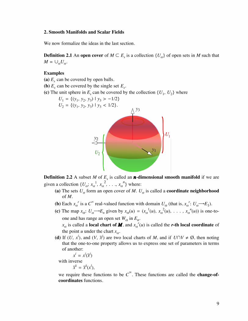
We now formalize the ideas in the last section. Definition 2.1 An open cover of M ¯ˉ Es is a collection {Uå} of open sets in M such that M = ÆåUå. Examples (a) Es can be covered by open balls. (b) Es can be covered by the single set Es. (c) The unit sphere in Es can be covered by the collection {U1, U2} where U1 = {(y1, y2, y3) | y3 > -1/2} U2 = {(y1, y2, y3) | y3 < 1/2}.

Definition 2.2 A subset M of Es is called an n-dimensional smooth manifold if we are given a collection {Uå; xå

1, xå2, . . ., xå

n} where: (a) The sets Uå form an open cover of M. Uå is called a coordinate neighborhood

of M. (b) Each xå

r is a CÏ real-valued function with domain Uå (that is, xår: Uå’E1).

(c) The map xå: Uå’En given by xå(u) = (xå1(u), xå

2(u), . . . , xån(u)) is one-to-

one and has range an open set Wå in En. xå is called a local chart of M , and xå

r(u) is called the r-th local coordinate of the point u under the chart xå.

(d) If (U, xi), and (V, x–j) are two local charts of M, and if UÚV ≠ Ø, then noting that the one-to-one property allows us to express one set of parameters in terms of another:

xi = xi(x–j) with inverse

x–k = x–k(xl),

we require these functions to be CÏ. These functions are called the change-of-coordinates functions.

10

The collection of all charts is called a smooth atlas of M . The “big” space Es in which the manifold M is embedded is the ambient space. Notes 1. Always think of the xi as the local coordinates (or parameters) of the manifold. We can paramaterize each of the open sets U by using the inverse function x-1 of x, which assigns to each point in some open set of En a corresponding point in the manifold. 2. Condition (d) implies that

det ⎝⎜⎛

⎠⎟⎞∂x–i

∂xj ≠ 0,

and

det ⎝⎜⎛

⎠⎟⎞∂xi

∂x–j ≠ 0,

since the associated matrices must be invertible. 3. The ambient space need not be present in the general theory of manifolds; that is, it is possible to define a smooth manifold M without any reference to an ambient space at all—see any text on differential topology or differential geometry (or look at Rund's appendix). 4. More terminology: We shall sometimes refer to the xi as the local coordinates, and to the yj as the ambient coordinates. Thus, a point in an n-dimensional manifold M in Es has n local coordinates, but s ambient coordinates. 5. For each å, we have put all the coordinate functions xå

r: Uå’E1 together to get a single map

11

xå: Uå’Wå ¯ˉ En. A more elegant formulation of conditions (c) and (d) above is then the following: each Wå is an open subset of En, each xå is invertible, and each composite

Wå -’xå

-1 En -’

x∫ W∫

is smooth. Examples 2.3 (a) En is an n-dimensional manifold, with the single identity chart defined by xi(y1, . . . , yn) = yi. (b) S1, the unit circle is a 1-dimensional manifold with charts given by taking the argument. Here is a possible structure with two charts, as shown in the following figure.

One has x: S1-{(1, 0)}’E1 x–: S1-{(-1, 0)}’E1, with 0 < x, x– < 2π, and the change-of-coordinate maps are given by

x– = ⎩⎪⎨⎪⎧ x+π if x < π

x-π if x > π (See the figure for the two cases. ) and

x = ⎩⎪⎨⎪⎧ x–+π if x– < π

x–-π if x– > π . Notice the symmetry between x and x–. Also notice that these change-of-coordinate functions are only defined when ø ≠ 0, π. Further, ∂x–/∂x = ∂x/∂x– = 1.

12

Note also that, in terms of complex numbers, we can write, for a point p = eiz é S1, x = arg(z), x– = arg(-z). (c) Generalized Polar Coordinates Let us take M = Sn, the unit n-sphere, Sn = {(y1, y2, … , yn, yn+1) é En+1 | £iyi

2 = 1}, with coordinates (x1, x2, . . . , xn) with 0 < x1, x2, . . . , xn-1 < π and 0 < xn < 2π, given by y1 = cos x1 y2 = sin x1 cos x2 y3 = sin x1 sin x2 cos x3 … yn-1 = sin x1 sin x2 sin x3 sin x4 … cos xn-1 yn = sin x1 sin x2 sin x3 sin x4 … sin xn-1 cos xn yn+1 = sin x1 sin x2 sin x3 sin x4 … sin xn-1 sin xn In the homework, you will be asked to obtain the associated chart by solving for the xi. Note that if the sphere has radius r, then we can multiply all the above expressions by r, getting y1 = r cos x1 y2 = r sin x1 cos x2 y3 = r sin x1 sin x2 cos x3 … yn-1 = r sin x1 sin x2 sin x3 sin x4 … cos xn-1 yn = r sin x1 sin x2 sin x3 sin x4 … sin xn-1 cos xn yn+1 = r sin x1 sin x2 sin x3 sin x4 … sin xn-1 sin xn. (d) The torus T = S1¿S1, with four charts. The first is: x: (S1-{(1, 0)})¿(S1-{(1, 0)})’E2, given by x1((cosø, sinø), (cos˙, sin˙)) = ø x2((cosø, sinø), (cos˙, sin˙)) = ˙.

13

The remaining three charts are defined similarly by replacing one or both of (1, 0) by (-1, 0) (See the charts for S1.) The change-of-coordinate maps are omitted. (e) The cylinder (homework) (f) Sn, with (again) stereographic projection, is an n-manifold; the two charts are given as follows. Let P be the point (0, 0, . . , 0, 1) and let Q be the point (0, 0, . . . , 0, -1). Then define two charts (Sn-P, xi) and (Sn-Q, x–i) as follows (see the figure):

If (y1, y2, . . . , yn, yn+1) is a point in Sn, let

x1 = y1

1-yn+1 ; x–1 =

y1

1+yn+1 ;

x2= y2

1-yn+1 ; x–2 =

y2

1+yn+1 ;

. . . . . .

xn = yn

1-yn+1 . x–n =

yn

1+yn+1 .

We can invert these maps as follows: Let r2 = £i x

ixi, and r–2 = £i x–ix–i. Then:

y1 = 2x1

r2+1 ; y1 =

2x–1

1+r–2 ;

y2 = 2x2

r2+1 ; y2 =

2x–2

1+r–2 ;

. . . . . .

yn = 2xn

r2+1 ; yn =

2x–n

1+r–2 ;

14

yn+1 = r2-1r2+1

; yn+1 = 1-r–2

1+r–2 .

The change-of-coordinate maps are therefore:

x1 = y1

1-yn+1 =

2x–1

1+r–2

1 - 1-r–2

1+r–2 =

x–1

r–2 ; ...... (1)

x2 = x–2

r–2 ;

. . .

xn = x–n

r–2 .

This makes sense, since the maps are not defined when x–i = 0 for all i, corresponding to the north pole. Note Since r– is the distance from x–i to the origin, this map is “hyperbolic reflection” in the unit circle: Equation (1) implies that xi and x–i lie on the same ray from the origin, and

xi = 1r–

x–i

r– ; and squaring and adding gives

r = 1r– .

That is, project it to the circle, and invert the distance from the origin. This also gives the inverse relations, since we can write

x–i = r–2xi = xi

r2 .

In other words, we have the following transformation rules. Change of Coordinate Transformations for Stereographic Projection Let r2 = £i x

ixi, and r–2 = £i x–ix–i. Then

x–i = xi

r2

xi = x–i

r–2

rr– = 1 We now want to discuss scalar and vector fields on manifolds, but how do we specify such things? First, a scalar field:

15

Definition 2.4 A smooth scalar field on a smooth manifold M is just a smooth real-valued map ∞: M’E1. (In other words, it is a smooth function of the coordinates of M as a subset of Er.) Thus, ∞ associates to each point m of M a unique scalar ∞(m). If U is a subset of M, then a smooth scalar field on U is smooth real-valued map ∞: U’E1. If U ≠ M, we sometimes call such a scalar field local. If ∞ is a scalar field on M and x is a chart, then we can express ∞ as a smooth function ˙

of the associated parameters x1, x2, . . . , xn. If the chart is x–, we shall write ˙— for the function of the other parameters x–1, x–2, . . . , x–n. Note that we must have ˙ = ˙— at each point of the manifold (see the “transformation rule” below). Examples 2.5 (a) Let M = En (with its usual structure) and let ∞ be any smooth real-valued function in the usual sense. Then, using the identity chart, we have ∞ = ˙. (b) Let M = S2, and define ∞(y1, y2, y3) = y3. Using stereographic projection, we find both ˙ and ˙—:

˙(x1, x2) = y3(x1, x2) =

r2-1r2+1

= (x1)2 + (x2)2 - 1(x1)2 + (x2)2 + 1

—̇(x–1, x–2) = y3(x–1, x–2) =

1-r–2

1+r–2 =

1 - (x–1)2 - (x–2)2

1 + (x–1)2 + (x–2)2

(c) Local Scalar Field The most obvious candidate for local fields are the coordinate functions themselves. If U is a coordinate neighborhood, and x = {xi} is a chart on U, then the maps xi are local scalar fields. Sometimes, as in the above example, we may wish to specify a scalar field purely by specifying it in terms of its local parameters; that is, by specifying the various functions ˙ instead of the single function ∞. The problem is, we can't just specify it any way we want, since it must give a value to each point in the manifold independently of local coordinates. That is, if a point p é M has local coordinates (xj) with one chart and (x–h) with another, they must be related via the relationship x–j = x–j(xh). Transformation Rule for Scalar Fields —̇(x–j) = ˙(xh) whenever (xh) and (x–j) are the coordinates under x and x– of some point p in M. This formula can also be read as —̇(x–j(xh) ) = ˙(xh) Example 2.6 Look at Example 2.5(b) above. If you substituted x–i as a function of the xj, you would get ˙—(x–1, x–2) = ˙(x1, x2).

16

Exercise Set 2 1. Give the paraboloid z = x2 + y2 the structure of a smooth manifold. 2. Find a smooth atlas of E2 consisting of three charts. 3. (a) Extend the method in Exercise 1 to show that the graph of any smooth function f: E2’E1 can be given the structure of a smooth manifold. (b) Generalize part (a) to the graph of a smooth function f: En ’ E1. 4. Two atlases of the manifold M give the same smooth structure if their union is again a smooth atlas of M. (a) Show that the smooth atlases (E1, f), and (E1, g), where f(x) = x and g(x) = x3 are incompatible. (b) Find a third smooth atlas of E1 that is incompatible with both the atlases in part (a). 5. Consider the ellipsoid L ¯ˉ E3 specified by

x2

a2 + y2

b2 + z2

c2 = 1 (a, b, c ≠ 0).

Define f: L’S2 by f(x, y, z) = ⎝⎜⎛

⎠⎟⎞x

a, yb,

zc .

(a) Verify that f is invertible (by finding its inverse). (b) Use the map f, together with a smooth atlas of S2, to construct a smooth atlas of L. 6. Find the chart associated with the generalized spherical polar coordinates described in Example 2.3(c) by inverting the coordinates. How many additional charts are needed to get an atlas? Give an example. 7. Obtain the equations in Example 2.3(f).

17

3. Tangent Vectors and the Tangent Space We now turn to vectors tangent to smooth manifolds. We must first talk about smooth paths on M. Definition 3.1 A smooth path on M is a smooth map r: J→M, where J is some open interval. (Thus, r(t) = (y1(t), y2(t), . . ., ys(t) for t é J.) We say that r is a smooth path through m é M if r(t0) = m for some t0 é J. We can specify a path in M at m by its coordinates: y1 = y1(t), y2 = y2(t), . . . ys = ys(t), where m is the point (y1(t0), y2(t0), . . . , ys(t0)). Equivalently, since the ambient and local coordinates are functions of each other, we can also express a path—at least that part of it inside a coordinate neighborhood—in terms of its local coordinates: x1 = x1(t), x2 = x2(t), . . . xn = xn(t). Examples 3.2 (a) Smooth paths in En (b) A smooth path in S1, and Sn Definition 3.3 A tangent vector at m é M ¯ˉ Er is a vector v in Er of the form

v = y'(t0)

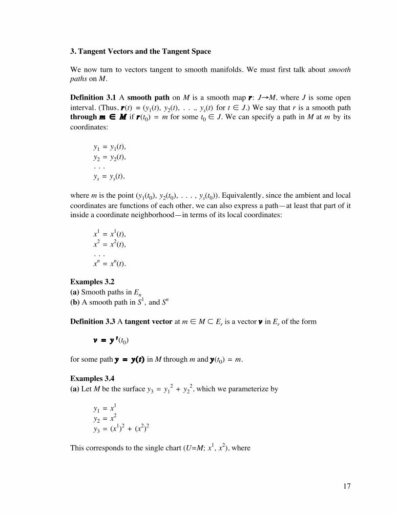
for some path y = y(t) in M through m and y(t0) = m. Examples 3.4 (a) Let M be the surface y3 = y1

2 + y22, which we parameterize by

y1 = x1 y2 = x2 y3 = (x1)2 + (x2)2 This corresponds to the single chart (U=M; x1, x2), where

18

x1 = y1 and x2 = y2. To specify a tangent vector, let us first specify a path in M, such as, for t é (0, +Ï) y1 = t sint y2 = t cost y3 = t (Check that the equation of the surface is satisfied.) This gives the path shown in the figure on the right.

Now we obtain a tangent vector field along the path by taking the derivative:

(dy1dt ,

dy2dt ,

dy3dt ) = ( t cost +

sint

2 t , - t sint +

cost2 t

, 1).

(To get actual tangent vectors at points in M, evaluate this at specific values of t.) Note We can also express the coordinates xi in terms of t: x1 = y1 = t sint x2 = y2 = t cost This descibes a path in some chart (that is, in coordinate space En) rather than on the mnanifold itself. We can also take the derivative,

(dx1

dt ,dx2

dt ) = ( t cost + sint

2 t , - t sint +

cost2 t

).

We also think of this as the tangent vector, given in terms of the local coordinates. A lot more will be said about the relationship between the above two forms of the tangent vector below. Algebra of Tangent Vectors: Addition and Scalar Multiplication The sum of two tangent vectors is, geometrically, also a tangent vector, and the same goes for scalar multiples of tangent vectors. However, we have defined tangent vectors using paths in M, and we cannot produce these new vectors by simply adding or scalar-multiplying the corresponding paths: if y = f(t) and y = g(t) are two paths through m é M where f(t0) = g(t0) = m, then adding them coordinate-wise need not produce a path in M. However, we can add these paths using some chart as follows:

19

Choose a chart x at m, with the property (for convenience) that x(m) = 0. Then the paths x(f(t)) and x(g(t)) (defined as in the note above) give two paths through the origin in coordinate space. Now we can add these paths or multiply them by a scalar without leaving coordinate space and then use the chart map to lift the result back up to M. In other words, define (f + g)(t) = x-1(x(f(t)) + x(g(t)) and (¬f)(t) = x-1(¬x(f(t))). Taking their derivatives at the point t0 will, by the chain rule, produce the sum and scalar multiples of the corresponding tangent vectors. Definition 3.5 If M is an n-dimensional manifold, and m é M, then the tangent space at m is the set Tm of all tangent vectors at m. Since we have equipped Tm with addition and scalar multiplication satisfying the “usual” properties, Tm has the structure of a vector space. Let us return to the issue of the two ways of describing the coordinates of a tangent vector at a point m é M: writing the path as yi = yi(t) we get the ambient coordinates of the tangent vector:

y'(t0) = (dy1

dt , dy2

dt , ..., dys

dt ) t=t0

Ambient coordinates

and, using some chart x at m, we get the local coordinates

x'(t0) = (dx1

dt , dx2

dt , ..., dxn

dt ) t=t0

Local Coordinates

Question In general, how are the dxi/dt related to the dyi/dt? Answer By the chain rule,

dy1dt =

∂y1

∂x1 dx1

dt + ∂y1

∂x2 dx2

dt + ... + ∂y1

∂xn dxn

dt

and similarly for dy2/dt ... dyn/dt. Thus, we can recover the original ambient vector coordinates from the local coordinates. In other words, the local vector coordinates completely specify the tangent vector. Note We use this formula to convert local coordinates to ambient coordinates:

20

Converting Between Local and Ambient Coordinates of a Tangent Vector If the tangent vector V has ambient coordinates (v1, v2, . . . , vs) and local coordinates (v1, v2, . . . , vn), then they are related by the formulæ

vi = ∑k=1

n

∂yi

∂xk vk

and

vi = ∑k=1

s

∂xi

∂yk vk

Note To obtain the coordinates of sums or scalar multiples of tangent vectors, simply take the corresponding sums and scalar multiples of the coordinates. In other words: (v+w)i = vi + wi and (¬v)i = ¬vI just as we would expect to do for ambient coordinates. (Why can we do this?) Examples 3.4 Continued: (b) Take M = En, and let v be any vector in the usual sense with coordinates åi. Choose x to be the usual chart xi = yi. If p = (p1, p2, . . . , pn) is a point in M, then v is the derivative of the path x1 = p1 + tå1 x2 = p2 + tå2; . . . xn = pn + tån at t = 0. Thus this vector has local and ambient coordinates equal to each other, and equal to

dxi

dt = åi, which are the same as the original coordinates. In other words, the tangent vectors are “the same” as ordinary vectors in En. (c) Let M = S2, and the path in S2 given by

21

y1 = sin t y2 = 0 y3 = cos t This is a path (circle) through m = (0, 0, 1) following the line of longitude ˙ = x2 = 0, and has tangent vector

(dy1dt ,

dy2dt ,

dy3dt ) = (cost, 0, -sint) = (1, 0, 0) at the point m.

(d) We can also use the local coordinates to describe a path; for instance, the path in part (c) can be described using spherical polar coordinates by x1 = t x2 = 0 The derivative

(dx1

dt ,dx2

dt ) = (1, 0) gives the local coordinates of the tangent vector itself (the coordinates of its image in coordinate Euclidean space). (e) In general, if (U; x1, x2, . . . , xn) is a coordinate system near m, then we can obtain paths yi(t) by setting

xj(t) = ⎩⎪⎨⎪⎧t + const. if j = iconst. if j ≠ i ,

where the constants are chosen to make xi(t0) correspond to m for some t0. (The paths in (c) and (d) are an example of this.) To view this as a path in M, we just apply the parametric equations yi = yi(x

j), giving the yi as functions of t. The associated tangent vector at the point where t = t0 is called ∂/∂xi. It has local coordinates

vj = ⎝⎜⎛

⎠⎟⎞dxj

dt t= t0

= ⎩⎪⎨⎪⎧1 if j = i0 if j ≠ i = ©i

j

©i

j is called the Kronecker Delta, and is defined by

22

©ij =

⎩⎪⎨⎪⎧1 if j = i0 if j ≠ i .

We can now get the ambient coordinates by the above conversion:

vj = ∑k=1

n

∂yj

∂xk vk = ∑

k=1

n

∂yj

∂xk ©ik =

∂yj

∂xi .

We call this vector ∂∂xi . Summarizing,

Definition of ∂∂xi

Pick a point m é M. Then ∂∂xi is the vector at m whose local coordinates under x are

given by

j th coordinate = ⎝⎜⎛

⎠⎟⎞∂

∂xi

j

= ©ij =

⎩⎪⎨⎪⎧1 if j = i0 if j ≠ i (Local coords of ∂/∂xi)

= ∂xj

∂xi

Its ambient coordinates are given by

j th coordinate = ∂yj

∂xi (Ambient coords of ∂/∂xi)

(everything evaluated at t0) Notice that the path itself has disappeared from the definition...

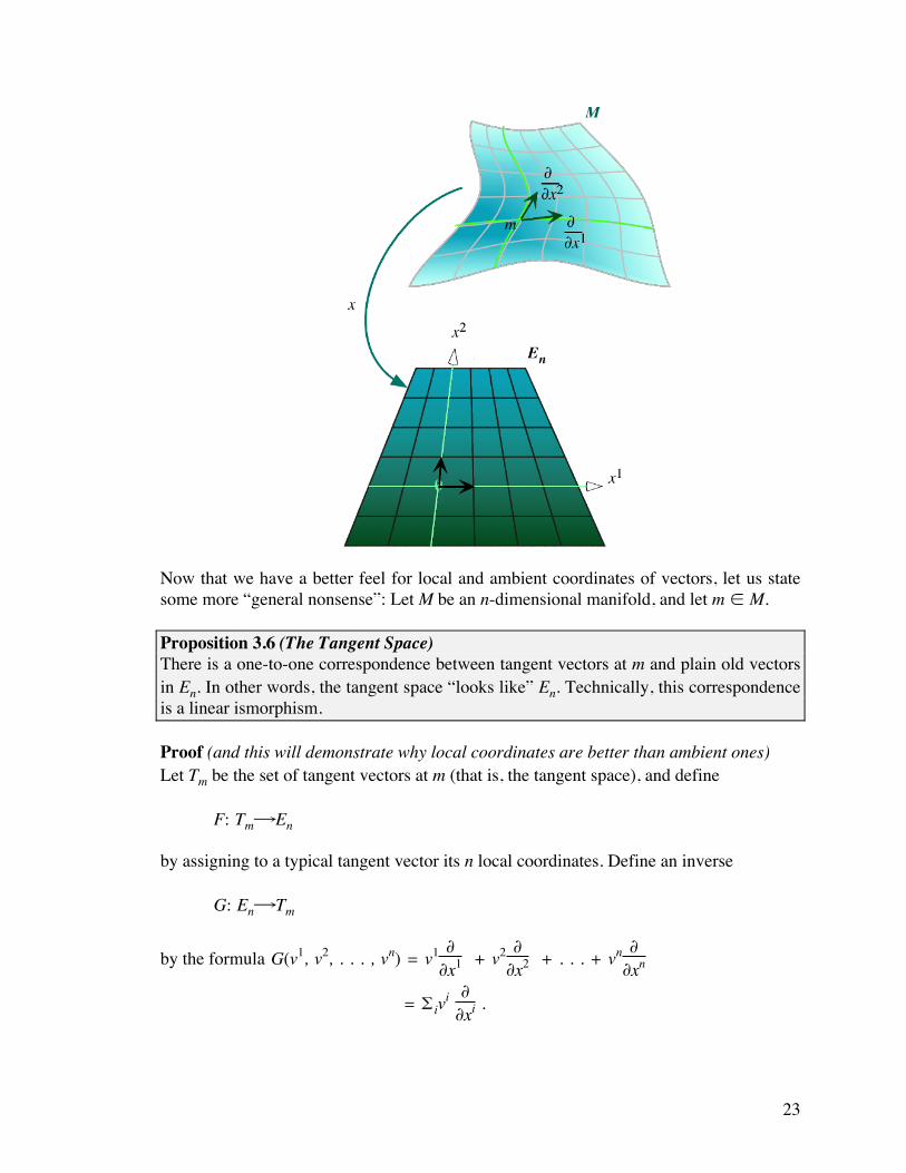
23

Now that we have a better feel for local and ambient coordinates of vectors, let us state some more “general nonsense”: Let M be an n-dimensional manifold, and let m é M. Proposition 3.6 (The Tangent Space) There is a one-to-one correspondence between tangent vectors at m and plain old vectors in En. In other words, the tangent space “looks like” En. Technically, this correspondence is a linear ismorphism. Proof (and this will demonstrate why local coordinates are better than ambient ones) Let Tm be the set of tangent vectors at m (that is, the tangent space), and define F: Tm’En by assigning to a typical tangent vector its n local coordinates. Define an inverse G: En’Tm

by the formula G(v1, v2, . . . , vn) = v1 ∂∂x1 + v2 ∂

∂x2 + . . . + vn ∂∂xn

= £ivi ∂∂xi .

24

Then we can verify that F and G are inverses as follows:

F(G(v1, v2, . . . , vn)) = F(£ivi ∂∂xi )

= local coordinates of the vector v1 ∂∂x1 + v2 ∂

∂x2 + . . . + vn ∂∂xn .

But, in view of the simple local coordinate structure of the vectors ∂∂xi , the i th coordinate

of this field is v1× 0 + . . . + vi-1× 0 + vi× 1 + vi+1× 0 + . . . + vn× 0 = vi. In other words, i th coordinate of F(G(v)) = F(G(v))i = vi, so that F(G(v)) = v. Conversely,

G(F(w)) = w1 ∂∂x1 + w2 ∂

∂x2 + . . . + wn ∂∂xn ,

where wi are the local coordinates of the vector w. Is this the same vector as w? Well, let us look at the ambient coordinates; since if two vectors have the same ambient coordinates, they are certainly the same vector! But we know how to find the ambient coordinates of each term in the sum. So, the j th ambient coordinate of G(F(w)) is

G(F(w))j = w1∂yj

∂x1 + w2∂yj

∂x2 + . . . + wn∂yj

∂xn

(using the formula for the ambient coordinates of the ∂/∂xi) = wj (using the conversion formulas) Therefore, G(F(w)) = w, and we are done. ✪

25

That is why we use local coordinates; there is no need to specify a path every time we want a tangent vector! Notes 3.7 (1) Under the one-to-one correspondence in the proposition, the standard basis vectors in En correspond to the tangent vectors ∂/∂x1, ∂/∂x2, . . . , ∂/∂xn. Therefore, the latter vectors are a basis of the tangent space Tm. (2) From the proof that G(F(w)) = w we see that, if w is any tangent vector with local coordinates wi, then: Expressing a Tangent vector in Terms of the ∂ /∂xn

w = £i wi ∂∂xi

Exercise Set 3 1. Suppose that v is a tangent vector at m é M with the property that there exists a local coordinate system xi at m with vi = 0 for every i. Show that v has zero coordinates in every coefficient system, and that, in fact, v = 0 . 2. (a) Calculate the ambient coordinates of the vectors ∂/∂ø and ∂/∂˙ at a general point

on S2, where ø and ˙ are spherical polar coordinates (ø = x1, ˙ = x2). (b) Sketch these vectors at some point on the sphere.

3. Prove that ∂∂x–i

= ∂xj

∂x–i ∂∂xj .

4. Consider the torus T2 with the chart x given by y1 = (a+b cos x1)cos x2 y2 = (a+b cos x1)sin x2 y3 = b sin x1

0 < xi < 2π. Find the ambeint coordinates of the two orthogonal tangent vectors at a general point, and sketch the resulting vectors.

26

4. Contravariant and Covariant Vector Fields Question How are the local coordinates of a given tangent vector for one chart related to those for another? Answer Again, we use the chain rule. The formula

dx–i

dt = ∂x–i

∂xj dxj

dt

(Note: we are using the Einstein Summation Convention: repeated index implies summation) tells us how the coordinates transform. In other words, we can think of a tangent vector at a point m in M as a collection of n numbers vi = dxi/dt (specified for each chart x at m) where the quantities for one chart are related to those for another according to the formula

v–i = ∂x–i

∂xj vj.

This leads to the following definition. Definition 4.1 A contravariant vector at m é M is a collection vi of n quantities (defined for each chart at m) which transform according to the formula

v–i = ∂x–i

∂xj vj.

It follows that contravariant vectors “are” just tangent vectors: the contravariant vector vi corresponds to the tangent vector given by

v = vi ∂∂xi ,

so we shall henceforth refer to tangent vectors as contravariant vectors. A contravariant vector field V on M associates with each chart x: U→W a collection of n smooth real-valued coordinate functions Vi of the n variables (x1, x2, . . . , xn), with domain W such that evaluating Vi at any point gives a vector at that point. Similarly, a contravariant vector field V on N ¯ˉ M is defined in the same way, but its domain is restricted to x(N)ÚW. Thus, the coordinates of a smooth vector field transform according to the way the individual vectors transform: Contravariant Vector Transformation Rule

V—i = ∂x–i

∂xj Vj

27

where now the Vi and V—j are functions of the associated coordinates (x1, x2, . . . , xn), rather than real numbers. Notes 4.2 (1) The above formula is reminiscent of matrix multiplication: In fact, if D— is the matrix

whose ij th entry is ∂x–i

∂xj , then the above equation becomes, in matrix form:

V— = D—V, where we think of V and V— as column vectors. (2) By “transform,” we mean that the above relationship holds between the coordinate functions Vi of the xi associated with the chart x, and the functions V—i of the x–i, associated with the chart x–. (3) Note the formal symbol cancellation: if we cancel the ∂'s, the x's, and the superscripts on the right, we are left with the symbols on the left! (4) In Notes 3.7 we saw that, if V is any smooth contravariant vector field on M, then

V = Vj ∂∂xj .

Examples 4.3 (a) Take M = En, and let F be any (tangent) vector field in the usual sense with coordinates Fi. If p = (p1, p2, . . . , pn) is a point in M, then F is the derivative of the path x1 = p1 + tF1 x2 = p2 + tF2; . . . xn = pn + tFn at t = 0. Thus this vector field has (ambient and local) coordinate functions

dxi

dt = Fi, which are the same as the original coordinates. In other words, the tangent vectors fields are “the same” as ordinary vector fields in En. (b) An Important Local Vector Field Recall from Examples 3.4 (e) above the definition of the vectors ∂/∂xi: At each point m in a manifold M, we have the n vectors ∂/∂x1, ∂/∂x2, . . . , ∂/∂xn, where the typical vector ∂/∂xi was obtained by taking the derivative of the path:

∂∂xi = vector obtained by differentiating the path xj(t) =

⎩⎪⎨⎪⎧t + const. if j = iconst. if j ≠ i ,

28

where the constants are chosen to make xi(t0) correspond to m for some t0. This gave

⎝⎜⎛

⎠⎟⎞∂

∂xi

j = © j

i (Coordinates under x)

Its coordinates under some other chart x– at m are then

© k i ∂x–j

∂xk = ∂x–j

∂xi (Coordinates under a general cahrt x)

If we now define the local vector fields ∂/∂x1, ∂/∂x2, . . . , ∂/∂xn to have the same coordinates under the general chart x–; viz:

⎝⎜⎛

⎠⎟⎞∂

∂xi

j = ∂x–j

∂xi

we see that it is defined everywhere on the domain U of x, so we get a local field defined on U. Notes (1) Geometrically, we can visualize this field by drawing, in the range of x, the constant field of unit vectrs pointing in the i direction.

(2) ∂∂xi is a field, and not the ith coordinate of a field.

Question Since the coordinates do not depend on x, does it mean that the vector field ∂/∂xi is constant? Answer No. Remember that a tangent field is a field on (part of) a manifold, and as such, it is not, in general, constant. The only thing that is constant are its coordinates under the specific chart x. The corresponding coordinates under another chart x– are ∂x–j/∂xi (which are not constant in general). (c) Extending Local Vector Fields The vector field in the above example has the disadvantage that is local. We can “extend” it to the whole of M by making it zero near the boundary of the coordinate patch, as follows. If m é M and x is any chart of M, lat x(m) = y and let D be a disc or some radius r centered at y entirely contained in the image of x. Now define a vector field on the whole of M by

w(p) = ⎩⎪⎨⎪⎧ ∂∂xj e-R2 if p is in D

0 otherwise

where

29

R = |x(p) - y|

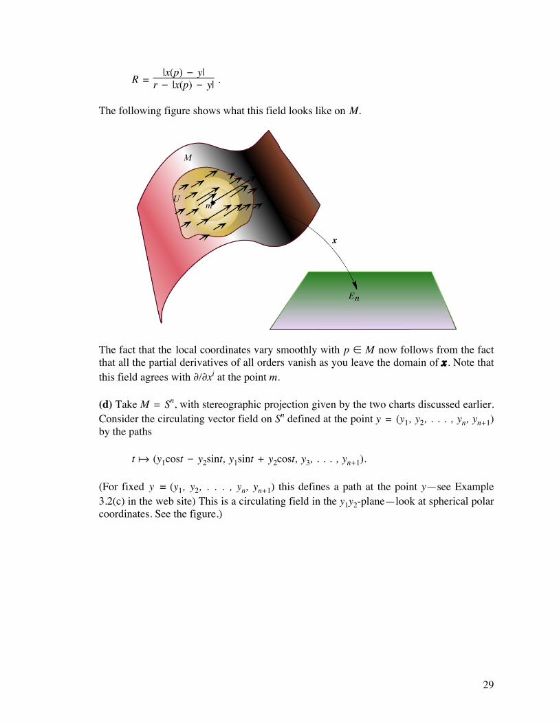
r - |x(p) - y| .

The following figure shows what this field looks like on M.

The fact that the local coordinates vary smoothly with p é M now follows from the fact that all the partial derivatives of all orders vanish as you leave the domain of x . Note that this field agrees with ∂/∂xi at the point m. (d) Take M = Sn, with stereographic projection given by the two charts discussed earlier. Consider the circulating vector field on Sn defined at the point y = (y1, y2, . . . , yn, yn+1) by the paths t (y1cost - y2sint, y1sint + y2cost, y3, . . . , yn+1). (For fixed y = (y1, y2, . . . , yn, yn+1) this defines a path at the point y—see Example 3.2(c) in the web site) This is a circulating field in the y1y2-plane—look at spherical polar coordinates. See the figure.)

30

(Note: Length of tangent vector = radius of circle)

In terms of the charts, the local coordinates of this field are:

x1 = y1

1-yn+1 =

y1cost - y2sint1-yn+1

; so V1 = dx1

dt = - y1sint + y2cost

1-yn+1 = - x2

x2 = y2

1-yn+1 =

y1sint + y2cost1-yn+1

; so V2 = dx2

dt = y1cost - y2sint

1-yn+1 = x1

x3 = y3

1-yn+1 ; so V3 =

dx3

dt = 0

. . .

xn = yn

1-yn+1 ; so Vn =

dxn

dt = 0.

and

x–1 = y1

1+yn+1 =

y1cost - y2sint1+yn+1

; so V—1 = dx–1

dt = - y1sint + y2cost

1+yn+1 = - x–2

x–2 = y2

1+yn+1 =

y1sint + y2cost1+yn+1

; so V—2 = dx–2

dt = y1cost - y2sint

1+yn+1 = x–1

x–3 = y3

1+yn+1 ; so V—3 =

dx–3

dt = 0

. . .

x–n = yn

1+yn+1 ; so V—n =

dx–n

dt = 0.

Now let us check that they transform according to the contravariant vector transformation rule. First, we saw above that

x–i = xi

r2 ,

and hence

31

∂x–i

∂xj =

⎩⎪⎨⎪⎧

r2-2(xi)2

r4 if j = i

-2xixj

r4 if j ≠ i .

In matrix form, this is:

D— = 1r4

⎣⎢⎢⎡

⎦⎥⎥⎤r2-2(x1)2 -2x1x2 -2x1x3 … -2x1xn

-2x2x1 r2-2(x2)2 -2x2x3 … -2x2xn

… … … … …-2xnx1 -2xnx2 -2xnx3 … r2-2(xn)2

Thus,

D—V = 1r4

⎣⎢⎢⎡

⎦⎥⎥⎤r2-2(x1)2 -2x1x2 -2x1x3 … -2x1xn

-2x2x1 r2-2(x2)2 -2x2x3 … -2x2xn

… … … … …-2xnx1 -2xnx2 -2xnx3 … r2-2(xn)2

⎣⎢⎢⎡

⎦⎥⎥⎤-x2

x1

00…0

= 1r4

⎣⎢⎢⎡

⎦⎥⎥⎤-x2r2 + 2(x1)2x2 - 2(x1)2x2

2(x2)2x1 + r2x1 - 2(x2)2x1

00…0

=

⎣⎢⎢⎡

⎦⎥⎥⎤-x2/r2

x1/r2

00…0

=

⎣⎢⎢⎡

⎦⎥⎥⎤-x–2

x–1

00…0

= V—.

Covariant Vector Fields We now look at the (local) gradient. If ˙ is a smooth scalar field on M, and if x is a chart, then we obtain the locally defined vector field ∂˙/∂xi. By the chain rule, these functions transform as follows:

∂˙∂x–i

= ∂˙∂xj

∂xj

∂x–i ,

or, writing Ci = ∂˙/∂xi,

C—i =∂xj

∂x–i Cj .

This leads to the following definition. Definition 4.4 A covariant vector field C on M associates with each chart x a collection of n smooth functions Ci(x

1, x2, . . . , xn) which satisfy:

32

Covariant Vector Transformation Rule

C—i = Cj ∂xj

∂x–i

Notes 4.5

1. If D is the matrix whose ij th entry is ∂xi

∂x–j , then the above equation becomes, in matrix

form: C— = CD, where now we think of C and C— as row vectors. 2. Note that

(DD—)ij = ∂xi

∂x–k ∂x–k

∂xj = ∂xi

∂xj = ©ij,

and similarly for D—D. Thus, D— and D are inverses of each other. 3. Note again the formal symbol cancellation: if we cancel the ∂'s, the x's, and the superscripts on the right, we are left with the symbols on the left! 4. Guide to memory: In the contravariant objects, the barred x goes on top; in covariant vectors, on the bottom. In both cases, the non-barred indices match. Question Geometrically, a contravariant vector is a vector that is tangent to the manifold. How do we think of a covariant vector? Answer The key to the answer is this: Definition 4.6 A smooth 1-form, or smooth cotangent vector field on the manifold M (or on an open subset U of M) is a function F that assigns to each smooth tangent vector field V on M (or on an open subset U) a smooth scalar field F(V), which has the following properties: F(V+W) = F(V) + F(W) F(åV) = åF(V). for every pair of tangent vector fields V and W , and every scalar å. (In the language of linear algebra, this says that F is a linear transformation.) Proposition 4.7 (Covariant Fields are One-Form Fields) There is a one-to-one correspondence between covariant vector fields on M (or U) and 1-forms on M (or U). Thus, we can think of covariant tangent fields as nothing more than 1-forms. Proof Here is the one-to-one correspondence. Let F be the family of 1-forms on M (or U) and let C be the family of covariant vector fields on M (or U). Define

33

∞: C’F by ∞(Ci)(V

j) = CkVk.

In the homework, we see that CkV

k is indeed a scalar by checking the transformation rule: C—kV—k = ClV

l. The linearity property of ∞ now follows from the distributive laws of arithmetic. We now define the inverse §: F’C by (§(F))i = F(∂/∂xi). We need to check that this is a smooth covariant vector field; that is, that is local components are smooth functions of the local coordinates and that it transforms in the correct way. Smoothness follows from the fact that each F(∂/∂xi) is a smooth scalar field and hence a smooth function of the local coordinates. For the transformation property, if x and x– are two charts, then

F(∂∂x–i

) = F( ∂xj

∂x–i ∂∂xj ) (The local coordinates under x of ∂/∂x–i are ∂xj/∂x–i)

= ∂xj

∂x–i F(

∂∂xj ),

by linearity. That § and ∞ are in fact inverses is left to the exercise set. ❉ Examples 4.8 (a) Let M = S1 with the charts: x = arg(z), x– = arg(-z) discussed in §2. There, we saw that the change-of-coordinate maps are given by

x = ⎩⎪⎨⎪⎧ x–+π if x– ≤ π

x–-π if x– ≥ π x– = ⎩⎪⎨⎪⎧ x+π if x ≤ π

x-π if x ≥ π , with ∂x–/∂x = ∂x/∂x– = 1, so that the change-of-coordinates do nothing. It follows that functions C and C— specify a covariant vector field iff C = C—. (Then they are automatically a contravariant field as well). For example, let C(x) = 1 = C—(x–).

34

This field circulates around S1. On the other hand, we could define C(x) = sin x and C—(x–) = - sin x– = sin x. This field is illustrated in the following figure:

(The length of the vector at the point eiø is given by sin ø.) (b) Let ˙ be a scalar field. Its ambient gradient, grad ˙, is given by

grad ˙ = ⎡⎣∂˙∂y1

, ... , ∂˙∂ys

⎤⎦,

that is, the garden-variety gradient you learned about in calculus. This gradient is, in general, neither covariant or contravariant. However, we can use it to obtain a 1-form as follows: If V is any contravariant vector field, then the rate of change of ˙ along V is given by V .grad ˙. (If V happens to be a unit vector at some point, then this is the directional derivative at that point.) In other words, dotting with grad ˙ assigns to each contravariant vector field the scalar field F(v) = V .grad ˙ which tells it how fast ˙ is changing along V . We also get the 1-form identities: F(V+W) = F(V) + F(W) F(åV) = åF(V). The coordinates of the corresponding covariant vector field are F(∂/∂xi) = (∂/∂xi).grad ˙

= [∂y1∂xi ,

∂y2∂xi , . . . ,

∂ys∂xi ] . [

∂˙∂y1

, , . . . , ∂˙∂ys

],

= ∂˙∂xi , which is the example that first motivated the definition. (c) Generalizing (b), let £ be any smooth vector field (in Es) defined on M. Then the operation of dotting with £ is a linear function from smooth tangent fields on M to

35

smooth scalar fields. Thus, it is a cotangent field on M with local coordinates given by applying the linear function to the canonical charts ∂/∂xi:

Ci = ∂∂xi ·£ .

The gradient is an example of this, since we are taking £ = grad ˙ in the preceding example. Note that, in general, dotting with £ depends only on the tangent component of £ . This leads us to the next example. (d) If V is any tangent (contravariant) field, then we can appeal to (c) above and obtain an associated covariant field. The coordinates of this field are not the same as those of V. To find them, we write:

V = Vi ∂∂xi (See Note 4.2 (4).)

Hence,

Cj = ∂∂xj ·Vi ∂

∂xi = Vi ∂∂xj ·

∂∂xi .

Note that the tangent vectors ∂/∂xi are not necessarily orthogonal, so the dot products

don't behave as simply as we might suspect. We let gij = ∂∂xj ·

∂∂xi , so that

Cj = gijVi.

We shall see the quantities gij again presently. Definition 4.9 If V and W are contravariant (or covariant) vector fields on M, and if å is a real number, we can define new fields V+W and åV by (V + W)i = Vi + Wi and (åV)i = åVi. It is easily verified that the resulting quantities are again contravariant (or covariant) fields. (Exercise Set 4). For contravariant fields, these operations coincide with addition and scalar multiplication as we defined them before. These operations turn the set of all smooth contravariant (or covariant) fields on M into a vector space. Note that we cannot expect to obtain a vector field by adding a covariant field to a contravariant field.

36

Exercise Set 4 1. Suppose that Xj is a contravariant vector field on the manifold M with the following property: at every point m of M, there exists a local coordinate system xi at m with Xj(x1, x2, . . . , xn) = 0. Show that Xi is identically zero in any coordinate system. 2. Give and example of a contravariant vector field that is not covariant. Justify your claim. 3. Verify the following claim If V and W are contravariant (or covariant) vector fields on M, and if å is a real number, then V+W and åV are again contravariant (or covariant) vector fields on M. 4. Verify the following claim in the proof of Proposition 4.7: If Ci is covariant and Vj is contravariant, then CkV

k is a scalar. 5. Let ˙: Sn’E1 be the scalar field defined by ˙(p1, p2, . . . , pn+1) = pn+1. (a) Express ˙ as a function of the xi and as a function of the x–j (the charts for stereographic projection). (b) Calculate Ci = ∂˙/∂xi and C—j = ∂˙/∂x–j. (c) Verify that Ci and C—j transform according to the covariant vector transformation rules. 6. Is it true that the quantities xi themselves form a contravariant vector field? Prove or give a counterexample. 7. Prove that § and ∞ in Proposition 4.7 are inverse functions. 8. Prove: Every covariant vector field is of the type given in Example 4.8(d). That is, obtained from the dot product with some contrravariant field.

37

5. Tensor Fields Suppose that v = “v1, v2, v3‘ and w = “w1, w2, w3‘ are vector fields on E3. Then their tensor product is defined to consist of the nine quantities viwj. Let us see how such things transform. Thus, let V and W be contravariant, and let C and D be covariant. Then:

V—iW—j = ∂x–i

∂xk Vk ∂x–j

∂xl Wl = ∂x–i

∂xk ∂x–j

∂xl VkWl,

and similarly,

V—iC—j = ∂x–i

∂xk ∂xl

∂x–j VkCl ,

and

C—iD—j = ∂xk

∂x–i ∂xl

∂x–j CkDl .

We call these fields “tensors” of type (2, 0), (1, 1), and (0, 2) respectively. Definition 5.1 A tensor field of type (2, 0) on the n-dimensional smooth manifold M associates with each chart x a collection of n2 smooth functions Sij(x1, x2, . . . , xn) which satisfy the transformation rules shown below. Similarly, we define tensor fields of type (0, 2), (1, 1), and, more generally, a tensor field of type (m, n). Some Tensor Transformation Rules

Type (2, 0): S—ij = ∂x–i

∂xk ∂x–j

∂xl Skl Matrix Form: S— = D—SD—T

Type (1, 1): M—ij = ∂x–i

∂xk ∂xl

∂x–j Mk

l Matrix Form: M— = D—MD

Type (0, 2): N—ij = ∂xk

∂x–i ∂xl

∂x–j Nkl Matrix Form: N— = DTND

Notes (1) A tensor field of type (1, 0) is just a contravariant vector field, while a tensor field of type (0, 1) is a covariant vector field. Similarly, a tensor field of type (0, 0) is a scalar field. Type (1, 1) tensors correspond to linear transformations in linear algebra. (2) We add and scalar multiply tensor fields in a manner similar to the way we do these things to vector fields. For instant, if A and B are type (1,2) tensors, then their sum is given by (A+B)ab

c = Aabc + Bab

c. Examples 5.2 (a) Of course, by definition, we can take tensor products of vector fields to obtain tensor fields, as we did above in Definition 4.1.

38

(b) The Kronecker Delta Tensor, given by

©ij =

⎩⎪⎨⎪⎧ 1 if j = i

0 if j ≠ i is, in fact a tensor field of type (1, 1). Indeed, one has

©ij =

∂xi

∂xj ,

and the latter quantities transform according to the rule

©—ij = ∂x–i

∂x–j = ∂x–i

∂xk ∂xk

∂xl ∂xl

∂x–j =

∂x–i

∂xk ∂xl

∂x–j ©k

l ,

whence they constitute a tensor field of type (1, 1). Notes:

(1) ©ij = ©—ij as functions on En. Also, ©i

j = ©ji . That is, it is a symmetric tensor.

(2) ∂x–i

∂xj ∂xj

∂x–k =

∂x–i

∂x–k = ©i

k .

Question OK, so is this how it works: Given a point p of the manifold and a chart x at p this strange object assigns the n2 quantities ©i

j ; that is, the identity matrix, regardless of the chart we chose? Answer Yes. Question But how can we interpret this strange object? Answer Just as a covariant vector field converts contravariant fields into scalars (see Section 3) we shall see that a type (1,1) tensor converts contravariant fields to other contravariant fields. This particular tensor does nothing: put in a specific vector field V, out comes the same vector field. In other words, it is the identity transformation.

(c) We can make new tensor fields out of old ones by taking products of existing tensor fields in various ways. For example, Mi

jk Npqrs is a tensor of type (3, 4),

while Mi

jk Njkrs is a tensor of type (1, 2).

Specific examples of these involve the Kronecker delta, and are in the homework.

(d) If X is a contravariant vector field, then the functions ∂Xi

∂xj do not define a tensor.

Indeed, let us check the transformation rule directly:

∂X—i

∂x–j = ∂∂x–j ⎝⎜

⎛⎠⎟⎞Xk∂x–

i

∂xk

= ∂∂xh ⎝⎜

⎛⎠⎟⎞Xk∂x–

i

∂xk ∂xh

∂x–j

= ∂Xk

∂xh ∂x–i

∂xk ∂xh

∂x–j + Xk ∂

2x–i

∂xh∂xK

39

The extra term on the right violates the transformation rules. We will see more interesting examples later. Proposition 5.3 (If It Looks Like a Tensor, It Is a Tensor) Suppose that we are given smooth local functions gij with the property that for every pair of contravariant vector fields Xi and Yi, the smooth functions gijX

iYj determine a scalar field, then the gij determine a smooth tensor field of type (0, 2). Proof Since the gijX

iYj form a scalar field, we must have g–ijX—iY—j = ghkX

hYk. On the other hand,

g–ijX—iY—j = g–ijXhYk∂x–

i

∂xh ∂x–j

∂xk .

Equating the right-hand sides gives

ghkXhYk = g–ij

∂x–i

∂xh ∂x–j

∂xk XhYk ---------------------- (I)

Now, if we could only cancel the terms XhYk. Well, choose a point m é M. It suffices to

show that ghk = g–ij∂x–i

∂xh ∂x–j

∂xk , when evaluated at the coordinates of m. By Example 4.3(c),

we can arrange for vector fields X and Y such that

Xi(coordinates of m) = ⎩⎪⎨⎪⎧ 1 if i = h

0 otherwise , and

Yi(coordinates of m) = ⎩⎪⎨⎪⎧ 1 if i = k

0 otherwise . Substituting these into equation (I) now gives the required transformation rule. ◆ Example 5.4 Metric Tensor Define a set of quantities gij by

gij = ∂∂xj ·

∂∂xi .

If Xi and Yj are any contravariant fields on M, then X ·Y is a scalar, and

X ·Y = Xi ∂∂xi ·Yj ∂

∂xj = gijXiYj.

Thus, by proposition 4.3, it is a type (0, 2) tensor. We call this tensor “the metric tensor inherited from the imbedding of M in Es.” Exercise Set 5 1. Compute the transformation rules for each of the following, and hence decide whether or not they are tensors. Sub-and superscripted quantities (other than coordinates) are understood to be tensors.

40

(a) dXi

jdt (b)

∂xi

∂xj (c) ∂Xi

∂xj (d) ∂2˙∂xi∂xj (e)

∂2xl

∂xi∂xj

2. (Rund, p. 95 #3.4) Show that if Aj is a type (0, 1) tensor, then

∂Aj

∂xh - ∂Ah

∂xj

is a type (0, 2) tensor. 3. Show that, if M and N are tensors of type (1, 1), then: (a) Mi

j Npq is a tensor of type (2, 2)

(b) Mij N

jq is a tensor of type (1, 1)

(c) Mij N

ji is a tensor of type (0, 0) (that is, a scalar field)

4. Let X be a contravariant vector field, and suppose that M is such that all change-of-coordinate maps have the form x–i = aijxj + ki for certain constants aij and kj. (We call

such a manifold affine.) Show that the functions ∂Xi

∂xj define a tensor field of type (1, 1).

5. (Rund, p. 96, 3.12) If Bijk = -Bjki, show that Bijk = 0. Deduce that any type (3, 0) tensor that is symmetric on the first pair of indices and skew-symmetric on the last pair of indices vanishes. 6. (Rund, p. 96, 3.16) If Akj is a skew-symmetric tensor of type (0, 2), show that the quantities Brst defined by

Brst = ∂Ast

∂xr + ∂Atr

∂xs + ∂Ars

∂xt

(a) are the components of a tensor; and (b) are skew-symmetric in all pairs in indices. (c) How many independent components does Brst have? 7. Cross Product (a) If X and Y are contravariant vectors, then their cross-product is defined as the tensor of type (2, 0) given by (X … Y)ij = XiYj - XjYi. Show that it is a skew-symmetric tensor of type (2, 0). (b) If M = E3, then the totally antisymmetric third order tensor is defined by œijk = ¡Error! (or equivalently, œ123 = +1, and œijk is skew-symmetric in every pair of indices.) Then, the (usual) cross product on E3 is defined by (X ¿ Y)i = œijkX

iYj = 12œijk(X … Y)ij

(c) What goes wrong when you try to define the “usual” cross product of two vectors on E4? Is there any analogue of (b) for E4? 8. Suppose that Cij is a type (2, 0) tensor, and that, regarded as an n¿n matrix C, it happens to be invertible in every coordinate system. Define a new collection of functions, Dij by taking

41

Dij = C-1ij,

the ij the entry of C-1 in every coordinate system. Show that Dij, is a type (0, 2) tensor. [Hint: Write down the transformation equation for Cij using matrix notation and invert everything in sight.]

9. What is wrong with the following “proof” that ∂2xj–

∂xh∂xk = 0 regardless of what smooth

functions x–j(xh) we use:

∂2xj–

∂xh ∂xk = ∂∂xh ⎝⎜

⎛⎠⎟⎞∂x–j

∂xk Definition of the second derivative

= ∂∂x–l ⎝⎜⎛

⎠⎟⎞∂x–j

∂xk ∂x–l

∂xh Chain rule

= ∂2xj–

∂x–l ∂xk ∂x–l

∂xh Definition of the second derivative

= ∂2xj–

∂xk ∂x–l ∂x–l

∂xh Changing the order of differentiation

= ∂∂xk ⎝⎜

⎛⎠⎟⎞∂x–j

∂x–l ∂x–l

∂xh Definition of the second derivative

= ∂∂xk ⎝

⎛⎠⎞©jl ∂x–l

∂xh Since ∂x–j

∂x–l = ©jl

= 0 Since ©il is constant!

42

6. Riemannian Manifolds Definition 6.1 A smooth inner product on a manifold M is a function “-,-‘ that associates to each pair of smooth contravariant vector fields X and Y a smooth scalar (field) “X, Y‘, satisfying the following properties. Symmetry: “X, Y‘ = “Y, X‘ for all X and Y, Bilinearity: “åX, ∫Y‘ = å∫“X, Y‘ for all X and Y, and scalars å and ∫ “X, Y+Z‘ = “X, Y‘ + “X, Z‘ “X+Y, Z‘ = “X, Z‘ + “Y, Z‘. Non-degeneracy: If “X, Y‘ = 0 for every Y, then X = 0. We also call such a gizmo a symmetric bilinear form. A manifold endowed with a smooth inner product is called a Riemannian manifold. Before we look at some examples, let us see how these things can be specified. First, notice that, if x is any chart, and p is any point in the domain of x , then

“X, Y‘ = XiYj“∂∂xi ,

∂∂xj ‘.

This gives us smooth functions

gij = “∂∂xi ,

∂∂xj ‘

such that “X, Y‘ = gijX

iYj and which, by Proposition 5.3, constitute the coefficients of a type (0, 2) symmetric tensor. We call this tensor the fundamental tensor or metric tensor of the Riemannian manifold. Note: From this point on, “field” will always mean “smooth field.” Examples 6.2 (a) M = En, with the usual inner product; gij = ©ij. (b) (Minkowski Metric) M = E4, with gij given (under the identity chart) by the matrix

G =

⎣⎢⎡

⎦⎥⎤1 0 0 0

0 1 0 00 0 1 00 0 0 -c2

,

where c is the speed of light. We call this Reimannian manifold flat Minkowski space M4. Question How does this effect the length of vectors? Answer We saw in Section 3 that, in En, we could think of tangent vectors in the usual way; as directed line segments starting at the origin. The role that the metric plays is that it tells you the length of a vector; in other words, it gives you a new distance formula:

43

Euclidean 3- space: d(x, y) = (y1 - x1)

2 + (y2 - x2)2 + (y3 - x3)

2

Minkowski 4-space: d(x, y) = (y1 - x1)2 + (y2 - x2)

2 + (y3 - x3)2 - c2(y4 - x4)

2 . Geometrically, the set of all points in Euclidean 3-space at a distance r from the origin (or any other point) is a sphere of radius r. In Minkowski space, it is a hyperbolic surface. In Euclidean space, the set of all points a distance of 0 from the origin is just a single point; in M, it is a cone, called the light cone. (See the figure.)

(c) If M is any manifold embedded in Es, then we have seen above that M inherits the structure of a Riemannian metric from a given inner product on Es. In particular, if M is any 3-dimensional manifold embedded in E4 with the metric shown above, then M inherits such a inner product. (d) As a particular example of (c), let us calculate the metric of the two-sphere M = S2, with radius r, using polar coordinates x1 = ø, x2 = ˙. To find the coordinates of g** we need to calculate the inner product of the basis vectors ∂/∂x1, ∂/∂x2. We saw in Section 3 that the ambient coordinates of ∂/∂xi are given by

j th coordinate = ∂yj

∂xi ,

where y1 = r sin(x1) cos(x2) y2 = r sin(x1) sin(x2) y3 = r cos(x1)

44

Thus,

∂∂x1 = r(cos(x1)cos(x2), cos(x1)sin(x2), -sin(x1))

∂∂x2 = r(-sin(x1)sin(x2), sin(x1)cos(x2), 0)

This gives g11 = “∂/∂x1, ∂/∂x1‘ = r2 g22 = “∂/∂x2, ∂/∂x2‘ = r2 sin2(x1) g12 = “∂/∂x1,∂/∂x2 ‘ = 0, so that

g** = ⎣⎢⎡

⎦⎥⎤r2 0

0 r2sin2(x1) .

(e) The n-Dimensional Sphere Let M be the n-sphere of radius r with the followihg generalized polar coordinates. y1 = r cos x1 y2 = r sin x1 cos x2 y3 = r sin x1 sin x2 cos x3 … yn-1 = r sin x1 sin x2 sin x3 sin x4 … cos xn-1 yn = r sin x1 sin x2 sin x3 sin x4 … sin xn-1 cos xn yn+1 = r sin x1 sin x2 sin x3 sin x4 … sin xn-1 sin xn. (Notice that x1 is playing the role of ø and the x2, x3, . . . , xn-1 the role of ˙.) Following the line of reasoning in the previous example, we have ∂∂x1 = (-r sin x1, r cos x1 cos x2, r cos x1 sin x2 cos x3 , . . . ,

r cos x1 sin x2… sin xn-1 cos xn, r cos x1 sin x2 … sin xn-1 sin xn) ∂∂x2 = (0, -r sin x1 sin x2, . . . , r sin x1 cos x2 sin x3… sin xn-1 cos xn,

r sin x1 cos x2 sin x3 … sin xn-1 sin xn). ∂∂x3 = (0, 0, -r sin x1 sin x2 sin x3, r sin x1 sin x2 cos x3 cos x4 . . . ,

r sin x1sin x2cos x3 sin x4…sin xn-1cos xn, r sin x1sin x2 cos x3sin x4 … sin xn-1sin xn),

45

and so on. g11 = “∂/∂x1, ∂/∂x1‘ = r2 g22 = “∂/∂x2, ∂/∂x2‘ = r2sin2x1

g33 = “∂/∂x3, ∂/∂x3‘ = r2sin2x1 sin2 x2

… gnn = “∂/∂xn, ∂/∂xn‘ = r2sin2x1 sin2

x2 … sin2 xn-1 gij = 0 if i ≠ j so that

g** =

⎣⎢⎡

⎦⎥⎤r2 0 0 … 0

0 r2sin2x1 0 … 00 0 r2sin2x1 sin2

x2 … 0… … … … …0 0 0 … r2sin2x1 sin2

x2 … sin2 xn-1

.

(f) Diagonalizing the Metric Let G be the matrix of g** in some local coordinate system, evaluated at some point p on a Riemannian manifold. Since G is symmetric and non-degenerate, it follows from linear algebra that there is an invertible matrix P = (Pji) such that

PGPT =

⎣⎢⎡

⎦⎥⎤±1 0 0 0

0 ±1 0 0… … … …0 0 0 ±1

at the point p. Let us call the sequence (±1, ±1, . . . , ±1) the signature of the metric at p. (Thus, in particular, a Minkowski metric has signature (1, 1, 1, -1).) If we now define new coordinates x–j by xi = x–j Pji (In matrix form: x = x –P, or x – = xP-1) then ∂xi/∂x–j = Pji, and so

g–ij = ∂xa

∂x–i gab∂xb

∂x–j = PiagabPjb

= Piagab(PT)bj = (PGPT)ij

showing that, at the point p,

46

g–** =

⎣⎢⎡

⎦⎥⎤±1 0 0 0

0 ±1 0 0… … … …0 0 0 ±1

.

Thus, in the eyes of the metric, the unit basis vectors ei = ∂/∂x–i are orthogonal; that is, “ei, ej‘ = ±©ij. Note The non-degeneracy condition in Definition 6.1 is equivalent to the requirement that the locally defined quantities g = det(gij) are nowhere zero. Here are some things we can do with a Riemannian manifold. Definition 6.3 If X is a contravariant vector field on M, then define the square norm of X by ||X||2 = “X, X‘ = gijX

iXj. Note that ||X||2 may be negative. If ||X||2 < 0, we call X timelike; if ||X||2 > 0, we call X spacelike, and if ||X||2 = 0, we call X null. If X is not spacelike, then we can define ||X|| = ||X||2 = gijX

iXj . In the exercise set you will show that null need not imply zero. Note Since “X, X‘ is a scalar field, so is ||X|| is a scalar field, if it exists, and satisfies ||˙X|| = |˙|·||X|| for every contravariant vector field X and every scalar field ˙. The expected inequality ||X + Y|| ≤ ||X|| + ||Y|| need not hold. (See the exercises.) Arc Length One of the things we can do with a metric is the following. A path C given by xi = xi(t) is non-null if ||dxi/dt||2 ≠ 0. It follows that ||dxi/dt||2 is either always positive (“spacelike”) or negative (“timelike”). Definition 6.4 If C is a non-null path in M, then define its length as follows: Break the path into segments S each of which lie in some coordinate neighborhood, and define the length of S by

47

L(a, b) = ⌡⎮⌠

a

b

± gijdxi

dtdxj

dt dt,

where the sign ±1 is chosen as +1 if the curve is space-like and -1 if it is time-like. In other words, we are defining the arc-length differential form by ds2 = ±gijdx

idxj. To show (as we must) that this is independent of the choice of chart x, all we need observe is that the quantity under the square root sign, being a contraction product of a type (0, 2) tensor with a type (2, 0) tensor, is a scalar. Proposition 6.5 (Paramaterization by Arc Length) Let C be a non-null path xi = xi(t) in M. Fix a point t = a on this path, and define a new function s (arc length) by s(t) = L(a, t) = length of path from t = a to t. Then s is an invertible function of t, and, using s as a parameter, ||dxi/ds||2 is constant, and equals 1 if C is space-like and -1 if it is time-like. Conversely, if t is any parameter with the property that ||dxi/dt||2 = ±1, then, choosing any parameter value t = a in the above definition of arc-length s, we have t = ±s + C for some constant C. (In other words, t must be, up to a constant, arc length. Physicists call the parameter † = s/c, where c is the speed of light, proper time for reasons we shall see below.) Proof Inverting s(t) requires s'(t) ≠ 0. But, by the Fundamental theorem of Calculus and the definition of L(a, t),

⎝⎜⎛

⎠⎟⎞ds

dt

2

= ± gijdxi

dtdxj

dt ≠ 0 for all parameter values t. In other words,

“ dxi

dt , dxi

dt ‘ ≠ 0. But this is the never null condition which we have assumed. Also,

48

“ dxi

ds , dxi

ds ‘ = gijdxi

dsdxj

ds = gijdxi

dtdxj

dt ⎝⎜⎛

⎠⎟⎞dt

ds

2

= ± ⎝⎜⎛

⎠⎟⎞ds

dt

2

⎝⎜⎛

⎠⎟⎞dt

ds

2

= ±1 For the converse, we are given a parameter t such that

“ dxi

dt , dxi

dt ‘ = ±1. in other words,

gijdxi

dtdxj

dt = ±1. But now, with s defined to be arc-length from t = a, we have

⎝⎜⎛

⎠⎟⎞ds

dt

2

= ± gijdxi

dtdxj

dt = +1 (the signs cancel for time-like curves) so that

⎝⎜⎛

⎠⎟⎞ds

dt

2

= 1, meaning of course that t = ±s + C. ❉ Examples 6.6 (a) A Non-Relativistic Closed Universe Take M = S4. Then we saw in Example 6.2(e) that we get

g** =

⎣⎢⎡

⎦⎥⎤

1 0 0 00 sin2x1 0 00 0 sin2x1 sin2x2 00 0 0 sin2x1 sin2x2 sin2x3

.

Think of x1 as time, and x2, 3, 4 as spatial coordinates. The point x1 = 0 is the “Big Bang” while the point x1 = π is the “Big Crunch.” Note that, as we approach these two points, the metric becomes singular, so we can think of it as a “singularity” in local space-time. At each time x1 = k strictly between 0 and π. the “universe” is a sphere of radius sin2x1. Then the length of an “around the universe cruise” on the “equator” of that sphere (x2 =

x3 = π/2) at a fixed moment x1 = k in time is the length of the path (x1, x2, x3, x4) = (k, π/2, π/2, t) (0 ≤ t ≤ 2π). Computing this amounts to integrating |sin x1 sin x2 sin x3| = sin k from 0 to 2π, giving us a total length of 2π sin k. Thusk the universe expands to a maximum at x1 = π/2 and then contracts back toward the Big Crunch.

49

Question What happened before the Big Bang in this universe (or after the Big Crunch)? Answer That is like asking “What lies north of the North Pole (or south of the South Pole)?” The best kind of person to answer that kind of question might be a Zen monk. (b) A Relativistic Expanding Universe Suppose that M is any 4-dimensional Riemannian manifold such that there is some chart x with respect to which the metric at a point p with local coordinates (x1, x2, x3, t) has the form

g** =

⎣⎢⎢⎡

⎦⎥⎥⎤

a(t)2 0 0 0

0 a(t)2 0 0

0 0 a(t)2 00 0 0 -1

(This time we are thinking of the last coordinate t as representing time. The reason for the squares is to ensure that the corresponding diagonal terms are non-negative. ) Note that we cannot use a change of coordinates to diagonalize the metric to one with signature (1, 1, 1, -1) unless we knew that a(t) ≠ 0 throughout. Again, if a(t) = 0 at some point, we have a singularity in space time. If, for instance, we take a(t) = tq, with 0 < q < 1 then t = 0 is a Big Bang (all distances are zero). Away from t = 0

ds2 = t2q[dx2 + dy2 + dz2] - dt2 so that distances expand forever in this universe. Also, at each time t ≠ 0, we can locally change coordinates to get a copy of flat Minkowski space M4. We will see later that this implies zero curvature away from the Big Bang, so we call this a flat universe with a singularity. Consider a particle moving in this universe: xi = xt(t) (yes we are using time as a parameter here). If the particle appears stationary or is traveling slowly, then (ds/dt)2 is negative, and we have a timelike path (we shall see that they correspond to particles traveling at sub-light speeds). When x· 2 + y· 2 + z·2 = t-2q (1) we find that (ds/dt)2 = 0, This corresponds to a null path (photons), and we think of t-q as the speed of light. (c = t-q so that c2 = t-2q). Think of h as ordinary distance measured at time t in our frame. Then (1) reduces, for a photon, to

50

dhdt = ± t-q

Integrating gives t = [±(1-q)(h-h0)]

1/(1-q) For simplicity let us take q = 1/2, so that the above curves give parabolas as shown:

Here, the Big Bang is represented by the horizontal (t = 0) axis. Only points inside a particular parabola are accessible from its vertex (h0, 0), by a signal at or below light-speed, so the points A and B in the picture are not in “causal contact” with each other. (Their futures so intersect, however.) Exercise Set 6 1. Give an example of a Riemannian metric on E2 such that the corresponding metric tensor gij is not constant. [Hint: Read Exercise #2.] 2. Let aij be the components of any symmetric tensor of type (0, 2) such that det(aij) is never zero. Define “X, Y‘a = aijX

iYj. Show that this is a smooth inner product on M. 3. Give an example to show that the “triangle inequality” ||X+Y|| ≤ ||X|| + ||Y|| is not always true on a Riemannian manifold. 4. Give an example of a Riemannian manifold M and a nowhere zero vector field X on M with the property that ||X|| = 0. We call such a field a null field. 5. Show that if g is any smooth type (0, 2) tensor field, and if g = det(gij) ≠ 0 for some chart x, then g– = det(g–ij) ≠ 0 for every other chart x– (at points where the change-of-coordinates is defined). [Use the property that, if A and B are matrices, then det(AB) = det(A)det(B).] 6. Suppose that gij is a type (0, 2) tensor with the property that g = det(gij) is nowhere zero. Show that the resulting inverse (of matrices) gij is a type (2, 0) tensor. [Hint: It is

51

suggested that you express all the transformation rules in terms of matrix notation -- see Exercise 8 in the preceding exercise set.] 7. (Index lowering and raising) Show that, if Rabc is a type (0, 3) tensor, then Ra

ic given

by Ra

ic = gibRabc,

is a type (1, 2) tensor. (Here, g** is the inverse of g**.) What is the inverse operation? 8. A type (1, 1) tensor field T is orthogonal in the Riemannian manifold M if, for all pairs of contravariant vector fields X and Y on M, one has “TX, TY‘ = “X, Y‘, where (TX)i = Ti

k Xk. What can be said about the columns of T in a given coordinate

system x? (Note that the ith column of T is the local vector field given by T(∂/∂xi).)

52

7. Locally Minkowskian Manifolds: An Introduction to Relativity First a general comment: We said in the last section that, at any point p in a Riemannian manifold M, we can find a local chart at p with the property that the metric tensor g** is diagonal at p, with diagonal terms ±1. In particular, we said that Minkowski space comes with a such a metric tensor having signature (1, 1, 1, -1). Now there is nothing special about the number 1 in the discussion: we can also find a local chart at any point p with the property that the metric tensor g** is diagonal, with diagonal terms any non-zero numbers we like (although we cannot choose the signs). In relativity, we deal with 4-dimensional manifolds, and take the first three coordinates x1, x2, x3 to be spatial (measuring distance), and the fourth one, x4, to be temporal (measuring time). Let us postulate that we are living in some kind of 4-dimensional manifold M (since we want to include time as a coordinate. By the way, we refer to a chart x at the point p as a frame of reference, or just frame). Suppose now we have a particle—perhaps moving, perhaps not—in M. Assuming it persists for a period of time, we can give it spatial coordinates (x1, x2, x3) at every instant of time (x4). Since the first three coordinates are then functions of the fourth, it follows that the particle determines a path in M given by x1 = x1(x4) x2 = x2(x4) x3 = x3(x4) x4 = x4, so that x4 is the parameter. This path is called the world line of the particle. Mathematically, there is no need to use x4 as the parameter, and so we can describe the world line as a path of the form xi = xi(t), where t is some parameter. (Note: t is not time; it's just a parameter. x4 is time). Conversely, if t is any parameter, and xi = xi(t) is a path in M, then, if x4 is an invertible function of t, that is, dx4/dt ≠ 0 (so that, at each time x4, we can solve for the other coordinates uniquely) then we can solve for x1, x2, x3 as smooth functions of x4, and hence picture the situation as a particle moving through space. Now, let's assume our particle is moving through M with world line xi = xi(t) as seen in our frame (local coordinate system). The velocity and speed of this particle (as measured in our frame) are given by

v = ⎝⎜⎛

⎠⎟⎞dx1

dx4 , dx2

dx4 , dx3

dx4

53

Speed2 = ⎝⎜⎛

⎠⎟⎞dx1

dx4

2

+ ⎝⎜⎛

⎠⎟⎞dx2

dx4

2

+ ⎝⎜⎛

⎠⎟⎞dx3

dx4

2

.

The problem is, we cannot expect v to be a vector—that is, satisfy the correct transformation laws. But we do have a contravariant 4-vector

Ti = dxi

dt (T stands for tangent vector. Also, remember that t is not time). If the particle is moving at the speed of light c, then

⎝⎜⎛

⎠⎟⎞dx1

dx4

2

+ ⎝⎜⎛

⎠⎟⎞dx2

dx4

2

+ ⎝⎜⎛

⎠⎟⎞dx3

dx4

2

= c2 ……… (I)

⇔ ⎝⎜⎛

⎠⎟⎞dx1

dt

2

+ ⎝⎜⎛

⎠⎟⎞dx2

dt

2

+ ⎝⎜⎛

⎠⎟⎞dx3

dt

2

= c2⎝⎜⎛

⎠⎟⎞dx4

dt

2

(using the chain rule)

⇔ ⎝⎜⎛

⎠⎟⎞dx1

dt

2

+ ⎝⎜⎛

⎠⎟⎞dx2

dt

2

+ ⎝⎜⎛

⎠⎟⎞dx3

dt

2

- c2⎝⎜⎛

⎠⎟⎞dx4

dt

2

= 0.

Now this looks like the norm-squared ||T||2 of the vector T under the metric whose matrix is

g** = diag[1, 1, 1, -c2] =

⎣⎢⎡

⎦⎥⎤1 0 0 0

0 1 0 00 0 1 00 0 0 -c2

In other words, the particle is moving at light-speed ⇔ ||T||2 = 0 ⇔ ||T|| is null under this rather interesting local metric. So, to check whether a particle is moving at light speed, just check whether T is null. Question What's the -c2 doing in place of -1 in the metric? Answer Since physical units of time are (usually) not the same as physical units of space, we would like to convert the units of x4 (the units of time) to match the units of the other axes. Now, to convert units of time to units of distance, we need to multiply by something with units of distance/time; that is, by a non-zero speed. Since relativity holds that the speed of light c is a universal constant, it seems logical to use c as this conversion factor. Now, if we happen to be living in a Riemannian 4-manifold whose metric diagonalizes to something with signature (1, 1, 1, -c2), then the physical property of traveling at the

54

speed of light is measured by ||T||2, which is a scalar, and thus independent of the frame of reference. In other words, we have discovered a metric signature that is consistent with the requirement that the speed of light is constant in all frames (at least in which g** has the above diagonal form). Definition 7.1 A Riemannian 4-manifold M is called locally Minkowskian if its metric has signature (1, 1, 1, -c2). For the rest of this section, we will be in a locally Minkowskian manifold M. Note If we now choose a chart x in locally Minkowskian space where the metric has the diagonal form diag[1, 1, 1, -c2] shown above at a given point p, then we have, at the point p: (a) If any path C has ||T||2 = 0, then

⎝⎜⎛

⎠⎟⎞dx1

dt

2

+ ⎝⎜⎛

⎠⎟⎞dx2

dt

2

+ ⎝⎜⎛

⎠⎟⎞dx3

dt

2

- c2⎝⎜⎛

⎠⎟⎞dx4

dt

2

= 0 (because this is how we calculate

||T||2) (b) If V is any contravariant vector with zero 4th-coordinate, then ||V||2 = (V1)2 + (V2)2 + (V3)2 (for the same reason as above) (a) says that we measure the world line C as representing a particle traveling with light speed, and (b) says that we measure ordinary length in the usual way. This motivates the following definition. Definition 7.2 A Lorentz frame at the point p é M is any chart x– at p with the following properties: (a) If any path C has the scalar ||T||2 = 0, then, at p,

⎝⎜⎛

⎠⎟⎞dx–1

dt

2

+ ⎝⎜⎛

⎠⎟⎞dx–2

dt

2

+ ⎝⎜⎛

⎠⎟⎞dx–3

dt

2

- c2⎝⎜⎛

⎠⎟⎞dx–4

dt

2

= 0 …… (II) (Note: “T—, T—‘ may not of this form in all frames because g–ij may not be be diagonal) (b) If V is a contravariant vector at p with V—4 = 0, then ||V||2 = (V—1)2 + (V—2)2 + (V—3)2 …… (III) (Note that, being a scalar, ||V||2 = ||V — ||2.) It follows from the remark preceding the defintion that if x is any chart such that, at the point p, the metric has the nice form diag[1, 1, 1, -c2], then x is a Lorentz frame at the point p. Note that in general, the coordinates of T in the system x–i are given by matrix

55

multiplication with some possibly complicated change-of-coordinates matrix, and to further complicate things, the metric may look messy in the new coordinate system. Thus, very few frames are going to be Lorentz. Physical Interpretation of a Lorentz Frame What the definition means physically is that an observer in the x–-frame who measures a particle traveling at light speed in the x-frame will also reach the conclusion that its speed is c, because he makes the decision based on (I), which is equivalent to (II). In other words: A Lorentz frame in locally Minkowskian space is any frame in which light appears to be

traveling at light speed, and where we measure length in the usual way. Question Do all Lorentz frames at p have the property that metric has the nice form diag[1, 1, 1, -c2]? Answer Yes, as we shall see below. Question OK. But if x and x– are two Lorentz frames at the point p, how are they related? Answer Here is an answer. First, continue to denote a specific Lorentz frame at the point p by x. Theorem 7.3 (Criterion for Lorentz Frames) Let M be locally Minkowskian, and let x be any frame such that, at p, G = diag[1, 1, 1, -c2] (so that x is a very nice Lorentz frame.) The following are equivalent: (a) A coordinate system x–i is Lorentz at the point p. (b) The columns of the change-of-coordinate matrix

Dji = ∂x–i

∂xj

satisfy “column i, column j‘ = “ei, ej‘, using the inner product defined by the matrix G. (c) G— = G, where G is as above. (This condition says that the change-of-coordinates transformation is a linear isometry of Minkowski space-time.) (d) If V is a contravariant vector at p, then ||V—||2 = (V—1)2 + (V—2)2 + (V—3)2 - c2(V—4)2. Proof (a) ⇒ (b) Suppose the coordinate system x–i is Lorentz at p, and let x be as hypothesized. We proceed by invoking condition (a) of Definition 7.2 for several paths. (These paths will correspond to sending out photons in various directions.) Path C : x1 = ct; x2 = x3 = 0, x4 = t (a photon traveling along the x1-axis in the local chart). This gives us a contravariant vector

56

T = (c, 0, 0, 1), with ||T||2 = 0, and so Definition 7.2 (a) applies to its coordinates in the (other) Lorentz frame x–. Let D be the change-of-basis matrix from x to x–;

Dki = ∂x–i

∂xk , (That is, D = D— in our usual notation)

so that T—i = Dk

iTk

=

⎣⎢⎢⎡

⎦⎥⎥⎤D1

1 D12 D1

3 D14

D21 D2

2 D23 D2

4

D31 D3

2 D33 D3

4

D41 D4

2 D43 D4

4

⎣⎢⎢⎡

⎦⎥⎥⎤c

001

.

By property (a) of Definition 7.2, (T—1)2 + (T—1)2 + (T—1)2 - c2(T—1)2 = 0, so that (cD1

1 + D14)

2 + (cD12 + D2

4)2 + (cD1

3 + D34)

2 - c2(cD14 + D4

4)2 = 0 … (*)

If we reverse the direction of the photon, we similarly get (-cD1

1 + D14)

2 + (-cD12 + D2

4)2 + (-cD1

3 + D34)

2 - c2(-cD14 + D4

4)2 = 0 …(**)

Noting that this only effects cross-terms, subtracting and dividing by 4c gives D1

1D14 + D1

2D24 + D1

3D34 - c2D1

4D44 = 0;

that is, “column 1, column 4‘ = 0 = “e1, e4‘. In other words, the first and fourth columns of D are orthogonal under the G. Similarly, by sending light beams in the other directions, we see that the other columns of D are orthogonal to the fourth column. If, instead of subtracting, we now add (*) and (**), and divide by 2, we get c2[D1

1D11 + D1

2 D12 + D1

3 D13 - c2D1

4 D14]

+ [D41D4

1 + D42 D4

2 + D43 D4

3 - c2D44 D4

4] = 0, showing that c2“column 1, column 1‘ = -“column 4, column 4‘.

57

So, if we write “column 1, column 1‘ = k, then “column 4, column 4‘ = -c2k … (***) Similarly (by choosing other photons) we can replace column 1 by either column 2 or column 3, showing that if we take “column 1, column 1‘ = k, we have

“column i, column i‘ = ⎩⎪⎨⎪⎧k if 1 ≤ i ≤ 3

-kc2 if i = 4 .

Let us now take another, more interesting, photon given by Path D: x1 = (c/ 2 )t; x2 = -(c/ 2 )t; x3 = 0; x4 = t, with T = “c/ 2 , -c/ 2 , 0, 1‘. (You can check to see that ||T||2 = 0, so that it does indeed represent a photon.) Since ||T—||2 = 0, we get (D1

1c / 2 - D21c / 2 +D4

1)2 + (D12c / 2 - D2

2c / 2 +D42)2

+ (D13c / 2 - D2

3c / 2 +D43)2 - c2(D1

4c / 2 - D24c / 2 +D4

4)2= 0 and, looking at a similar photon with reversed x2-coordinate, (D1

1c / 2 + D21c/ 2 +D4

1)2 + (D12c/ 2 + D2

2c/ 2 +D42)2

+ (D13c/ 2 + D2

3c/ 2 +D43)2 - c2(D1

4c/ 2 + D24c/ 2 +D4

4)2= 0 Subtracting these gives 2c2[D1

1D21 + D1

2 D22 + D1

3 D23 - c2D1

4 D24]

+ 4c/ 2 [D21D4

1 + D22 D4

2 + D23 D4

3 - c2D24 D4

4] = 0. But we already know that the second term vanishes, so we are left with D1

1D21 + D1

2 D22 + D1

3 D23 - c2D1

4 D24 = 0,

58

showing that columns 1 and 2 are also orthogonal. Choosing similar photons now shows us that columns 1, 2, and 3 are mutually orthogonal. Therefore, we have

“column i, columnj‘ =

⎩⎪⎨⎪⎧

0 if i ≠ j

k if 1 ≤ i = j ≤ 3

-kc2 if i = j = 4

. ..... (IV)

But, what is k? Let us invoke condition (b) of Defintion 7.2. To measure the length of a vector in the new frame, we need to transform the metric tensor using this coordinate change. Recall that, using matrix notation, the metric G transforms to G— = PTGP, where P is the matrix inverse of D above. In the exercise set, you will show that the columns of P have the same property (IV) above, but with k replaced by 1/k. But, G— = PTGP Now, G is just a constant multiple of an elementary matrix, and all it does is multiply the last row of P by -c2 and then multiply everything by 1/k. So, when we compute PT(GP), we are really getting a multiple of the funny scalar product of the columns of P back again, which just gives a multiple of G. In other words, we get G— = PTGP = G/k. Now we invoke condition (b) in Definition 7.2: Take the vector V— = (1, 0, 0, 0) in the x–-frame. (Recognize it? It is the vector ∂/∂x–1.) Since its 4th coordinate is zero, condition (b) says that its norm-squared must be given by the usual length formula: ||V—||2 = 1. On the other hand, we can also use G— to compuate ||V—||2, and we get

||V—||2 = 1k ,

showing that k = 1. Hence, G— = G, and also D has the desired form. This proves (b) (and also (c), by the way). (b) ⇒ (c) If the change of coordinate matrix has the above orthogonality property,

59

Di1Dj

1 + Di2 Dj

2 + Di3 Dj

3 - c2Di4 Dj

4 =

⎩⎪⎨⎪⎧

0 if i ≠ j

1 if 1 ≤ i = j ≤ 3

-c2 if i = j = 4

then the argument in (a) ⇒ (b) shows that G— = G (since k = 1/k = 1 here). (c) ⇒ (d) If G— = diag[1, 1, 1, -c2] at the point p, then, by definition of the norm-squared, ||V—||2 = (V—1)2 + (V—2)2 + (V—3)2 - c2(V—4)2. (d) ⇒ (a) a fortiori, as dxi/dt is a contravariant vector. ❊ We will call the transformation from one Lorentz frame to another a generalized Lorentz transformation. An Example of a Lorentz Transformation We would like to give a simple example of such a transformation matrix D, so we look for a matrix D whose first column has the general form “a, 0, 0, b‘, with a and b non-zero constants. (Why? If we take b = 0, we will wind up with a less interesting transformation: a rotation in 3-space.) There is no loss of generality in taking a = 1, so let us use “1, 0, 0, -∫/c‘. Here, c is the speed of light, and ∫ is a certain constant. (The meaning of ∫ will emerge in due course). Its norm-squared is (1 - ∫2), and we want this to be 1, so we replace the vector by

“ 1

1-∫2 , 0, 0, -

∫/c

1-∫2 ‘.

This is the first column of D. To keep things simple, let us take the next two columns to be the corresponding basis vectors e2, e3. Now we might be tempted to take the forth vector to be e4, but that would not be orthogonal to the above first vector. By symmetry (to get a zero inner product) we are forced to take the last vector to be

“- ∫c

1-∫2 , 0, 0,

1

1-∫2 ‘

This gives the transformation matrix as

60

D =

⎣⎢⎢⎢⎡

⎦⎥⎥⎥⎤

1

1-∫2 0 0 -

∫c

1-∫2

0 1 0 00 0 1 0

- ∫/c

1-∫2 0 0

1

1-∫2

.

and hence the new coordinates (by integrating everything in sight; using the boundary conditions x–i = 0 when xi = 0) as

x–1 = x1 - ∫cx4

1-∫2 ; x–2 = x2; x–3 = x3; x–4 =

x4 - ∫x1/c

1-∫2 .

Notice that solving the first equation for x1 gives x1 = x–1 1-∫2 + ∫cx4. Since x4 is just time t here, it means that the origin of the x–-system has coordinates (∫ct, 0, 0) in terms of the original coordinates. In other words, it is moving in the x-direction with a velocity of v = ∫c, so we must interpret ∫ as the speed in “warp;”

∫ = vc .

This gives us the famous Lorentz Transformations of Special Relativity If two Lorentz frames x and x– have the same coordinates at (x, y, z, t) = (0, 0, 0, 0), and if the x–-frame is moving in the x-direction with a speed of v, then the x–-coordinates of an event are given by

x– = x - vt

1-v2/c2 ; y– = y; z– = z; t – =

t - vx/c2

1-v2/c2

Remarks D above has the form

61

D =

⎣⎢⎢⎡

⎦⎥⎥⎤cosh ˙ 0 0 -c sinh ˙

0 1 0 00 0 1 0

-1c sinh ˙ 0 0 cosh ˙

and is therefore thought of as a “generalized hyperbolic rotation in 4-space.” Exercise Set 7 1. (a) What can be said about the scalar ||dxi/dt||2 in a Lorentz frame for a particle traveling at (i) sub-light speed (ii) super-light speed. (b) Conclude that, if a particle is traveling at super-light speed in one Lorentz frame, then it is traveling at super-light speeds in all such frames. 2. Show that, if xi(t) is a timelike path in the Minkowskian manifold M so that dx4/dt ≠ 0, then dx–4/dt ≠ 0 in every Lorentz frame x–. 3. Referring to the Lorentz transformations for special relativity, consider a “photon clock” constructed by bouncing a single photon back and forth bewtwwen two parallel mirrors as shown in in the following figure.

1 meter

tick tock

Now place this clock in a train moving in the x-direction with velocity v. By comparing the time it takes between a tick and a tock for a stationary observer and one on the train, obtain the time contraction formula (∆t– in terms ∆t) from the length contraction one. 4. Prove the claim in the proof of 7.3, that if D is a 4¿4 matrix whose columns satisfy

“column i, columnj‘ =

⎩⎪⎨⎪⎧

0 if i ≠ j

k if 1 ≤ i = j ≤ 3

-kc2 if i = j = 4

,

using the Minkowski inner product G (not the standard inner product), then D-1 has its columns satisfying

“column i, columnj‘ =

⎩⎪⎨⎪⎧

0 if i ≠ j

1/k if 1 ≤ i = j ≤ 3

-c2/k if i = j = 4

.

[Hint: Express the given property of D as a matrix equation involving G.] 5. Invariance of the Minkowski Form Show that, if P = xi

0 and Q = xi0 + ∆xi are any two events in the Lorentz frame xi, then,

for all Lorenz frames x–i, such that the change-of-coordinates matrix D is constant (as it is for special realtivity), one has

62

(∆x1)2 + (∆x2)2+ (∆x3)2- c2(∆x4)2 = (∆x–1)2 + (∆x–2)2+ (∆x–3)2- c2(∆x–4)2 [Hint: Consider the path xi(t) = x0

i + ∆xit, so that dxi/dt is independent of t. Now use the transformation formula to conclude that dx–i/dt is also independent of t. (You might have to transpose a matrix before multiplying…) Deduce that x–i(t) = zi + rit for some constants ri and si. Finally, set t = 0 and t = 1 to conclude that x–i(t) = x–0

i + ∆x–it, and apply (c) above.] 6. If the x–i-system is moving with a velocity v in a certain direction with resepct to the xi-system, we call this a boost in the given direction. Show that successive boosts in two perpendicular directions do not give a “pure” boost (the spatial axes are rotated—no longer parallel to the original axes). Now do some reading to find the transformation for a pure boost in an arbitrary direction.

63

8. Covariant Differentiation Intuitively, by a parallel vector field, we mean a vector field with the property that the vectors at different points are parallel. Is there a notion of a parallel field on a manifold? For instance, in En, there is an obvious notion: just take a fixed vector v and translate it around. On the torus, there are good candidates for parallel fields (see the figure) but not on the 2-sphere. (There are, however, parallel fields on the 3-sphere…)

Let us restrict attention to parallel fields of constant length. Usually, we can recognize such a field by taking the derivatives of its coordinates, or by following a path, and taking the derivative of the vector field with respect to t: we should come up with zero. The problem is, we won't always come up with zero if the coordinates are not rectilinear, since the vector field may change direction as we move along the curved coordinate axes. Technically, this says that, if Xj was such a field, we should check for its parallelism by taking the derivatives dXj/dt along some path xi = xi(t). However, there are two catches to this approach: one geometric and one algebraic. Geometric Look, for example, at the field on either torus in the above figure. Since it is circulating and hence non-constant, dX/dt ≠ 0, which is not what we want. However, the projection of dX/dt parallel to the manifold does vanish—we will make this precise below. Algebraic Since

X—j = ∂x–j

∂xh Xh,

one has, by the product rule,

dX—j

dt = ∂2x–j

∂xk∂xh Xh

dxk

dt + ∂x–j

∂xh dXh

dt , ........................ (I)

64

showing that, unless the second derivatives vanish, dX/dt does not transform as a vector field. What this means in practical terms is that we cannot check for parallelism at present—even in E3 if the coordinates are not linear. First, let us restrict to M is embedded in E

s with the metric inherited from the

embedding. The projection of dX/dt along M will be called the covariant derivative of X (with respect to t), and written DX/dt. To compute it, we need to do a little work. First, some linear algebra. Lemma 8.1 (Projection onto the Tangent Space) Let M ¯ˉ E

s be an n-manifold with metric g inherited from the embedding, and let V be a

vector in Es,. The projection πV of V onto Tm has (local) coordinates given by (πV)i = gik(V.∂/∂xk), where [gij] is the matrix inverse of [gij], and gij = (∂/∂xi).(∂/∂xj) as usual. Proof We can represent V as a sum,

V = πV + V⊥,

where V⊥ is the component of V normal to Tm. Now write ∂/∂xk as ek, and write πV = a1e1 + ... + anen, where the ai are the desired local coordinates. Then V = πV + V⊥ = a1e1 + ... + anen + V⊥ and so V·e1 = a1e1·e1 + ... + anen·e1 + 0 V·e2 = a1e1·e2 + ... + anen·e2 ... V·en = a1e1·en + ... + anen·en which we can write in matrix form as [V.ei] = [ai]g** whence [ai] = [V.ei]g**.

65

Finally, since g** is symmetric, we can transpose everything in sight to get [ai] = g**[V.ei], as required. Ì For reasons that will become clear later, let us now digress to look at some partial derivatives of the fundamental matrix [g**] in terms of ambient coordinates.

∂∂xp [gqr] =

∂∂xp ⎣

⎢⎡

⎦⎥⎤∂ys

∂xq ∂ys

∂xr

= ∂2ys

∂xp∂xq ∂ys

∂xr + ∂2ys

∂xr∂xp ∂ys

∂xq

or, using “comma notation”, gqr,p = ys,pq ys,r + ys,rp ys,q

Look now at what happens to the indices q, r, and p if we permute them (they're just letters, after all) cyclically in the above formula (that is, p→q→r), we get two more formulas.

gqr,p = ys,pq ys,r + ys,rp ys,q (Original formula) grp,q = ys,qr ys,p + ys,pq ys,r

gpq,r = ys,rp ys,q + ys,qr ys,p

Note that each term on the right occurs twice altogether as shown by the boxes and shading. This permits us to solve for the boxed term ys,pq ys,r by adding the first two equations and subtracting the third: ys,pq ys,r = 1

2 [ gqr,p + grp,q - gpq,r ]. ..... (*) Definition 8.2 Christoffel Symbols We make the following definitions.

[pq, r] = 12 [ gqr,p + grp,q - gpq,r ] Christoffel Symbols of the First Kind

⎩⎨⎧

⎭⎬⎫i

pq = gir [pq, r] Christoffel Symbols of the Second Kind

= 12 gir[ gqr,p + grp,q - gpq,r ]

Neither of these gizmos are tensors, but instead transform as follows (Which you will prove in the exercises!)

66

Transformation Law for Christoffel Symbols of the First Kind

[hk, l] = [ri, j] ∂x–r

∂xh ∂x–i

∂xk ∂x–j

∂xl + g–ij∂2x–i

∂xh∂xk ∂x–j

∂xl

Transformation Law for Christoffel Symbols of the Second Kind

⎩⎨⎧

⎭⎬⎫p

hk = ⎩⎨⎧

⎭⎬⎫t

ri ∂xp

∂x–t ∂x–r

∂xh ∂x–i

∂xk + ∂xp

∂x–t ∂2x–t

∂xh∂xk

(Look at how the patterns of indices match those in the Christoffel symbols...)

Proposition and Definition 8.2 (Formula for Covariant Derivative) (a) If M ¯ˉ E

s has the inherited metric, then

DXi

dt = dXi

dt + ⎩⎨⎧

⎭⎬⎫i

pq Xpdxq

dt

(b) If M is a completely general Riemannian manifold, then the DXi/dt as defined above (using the metric that comes with the manifold) is a contravariant vector, and so we define the covariant derivative using the above formula. Proof By definition,

DXdt = π

dXdt ,

which, by the lemma, has local coordinates given by

DXi

dt = gir

⎝⎜⎛

⎠⎟⎞dX

dt . ∂∂xr .

To evaluate the term in parentheses, we use ambeint coordinates. dX/dt has ambient coordinates

ddt ⎝⎜⎛

⎠⎟⎞

Xp∂y

s

∂xp = dXp

dt ∂y

s

∂xp + Xp ∂2ys

∂xp∂xq dxq

dt .

Thus, dotting with ∂/∂xk = ∂y

s/∂xr gives

dXp

dt ∂y

s

∂xp ∂y

s

∂xr + Xp ∂2ys

∂xp∂xq ∂y

s

∂xr dxq

dt

67

= dXp

dt gpr + Xp[pq, r]

dxq

dt . (By (*)) Finally,

DXi

dt = gir

⎝⎜⎛

⎠⎟⎞dX

dt . ∂∂xr

= gir ⎝⎜⎛

⎠⎟⎞dXp

dt gpr + Xp[pq, r]

dxq

dt

= ©ip dXp

dt + ⎩⎨⎧

⎭⎬⎫i

pq Xpdxq

dt (Defn of Christoffel symbols of the 2nd Kind)

= dXi

dt + ⎩⎨⎧

⎭⎬⎫i

pq Xpdxq

dt

as required. (b) In the exercises, you will check directly that the covariant derivative transforms correctly. Ì This allows us to say whether a field is parallel and of constant length by seeing whether this quantity vanishes. This claim is motivated by the following. Proposition 8.3 (Parallel Fields of Constant Length) Xi is a parallel field of constant length in En iff DXi/dt = 0 for all paths in En. Proof Designate the usual coordinate system by xi. Then Xi is parallel and of constant length iff its coordinates with respect to the chart x are constant; that is, iff

dXi

dt = 0. But, since for this coordinate system, gij = ©ij, the Christoffel symbols clearly vanish, and so

DXi

dt = dXi

dt = 0. But, if the contravariant vector DXi/dt vanishes under one coordinate system (whose domain happens to be the whole manifold) it must vanish under all of them. (Notice that we can't say that about things that are not vectors, such as dXi/dt.) ◆ Partial Derivatives Let xi = xi(t) be some path in M. Write

DXi

dt = dXi

dt + ⎩⎨⎧

⎭⎬⎫i

pq Xpdxq

dt

68

= ∂Xi

∂xq dxq

dt + ⎩⎨⎧

⎭⎬⎫i

pq Xpdxq

dt

= ⎣⎢⎡

⎦⎥⎤∂Xi

∂xq + ⎩⎨⎧

⎭⎬⎫i

pq Xp dxq

dt

The quantity in brackets converts the vector dxq/dt into the vector DXi/dt. Moreover, since every contravariant vector has the form dxq/dt for some path xi = xi(t) in M (recall the definition of tangent vectors in terms of paths), it follows that the quantity in brackets “looks like” a tensor of type (1, 1), and we call it the qth covariant partial derivative of Xi: Definition 8.4 The covariant partial derivative of the contravariant field Xp is the type (1, 1) tensor given by

Covariant Partial Derivative of Xi

Xi|q =

∂Xi

∂xq + ⎩⎨⎧

⎭⎬⎫i

pq Xp

(Some texts use ÔqX

i.) Do you see now why it is called the “covariant” derivative? Similarly, we can obtain the type (0, 2) tensor (check that it transforms correctly)

Covariant Partial Derivative of Yp

Yp|q = ∂Yp

∂xq -

⎩⎨⎧

⎭⎬⎫i

pq Yi

Notes 1. All these forms of derivatives satisfy the expected rules for sums and also products. (See the exercises.) 2. If C is a path on M, then we obtain the following analogue of the chain rule:

DXi

dt = Xp|kdxk

dt .

(See the definitions.) Examples 8.5 (a) Let M = En with the identity chart, so that gij = ©ij in the eyes of this chart. Since the Christoffel symbols involved the partial dervatives of the gij, they therefore vanish in the eyes of this chart, and so the coordinates of the covariant derivative DXi/dt are just those of dXi/dt. (b) Let M be the torus T, and think of T as obtained from the plane by identifying points as shown in the figure (each grid square is 2π×2π):

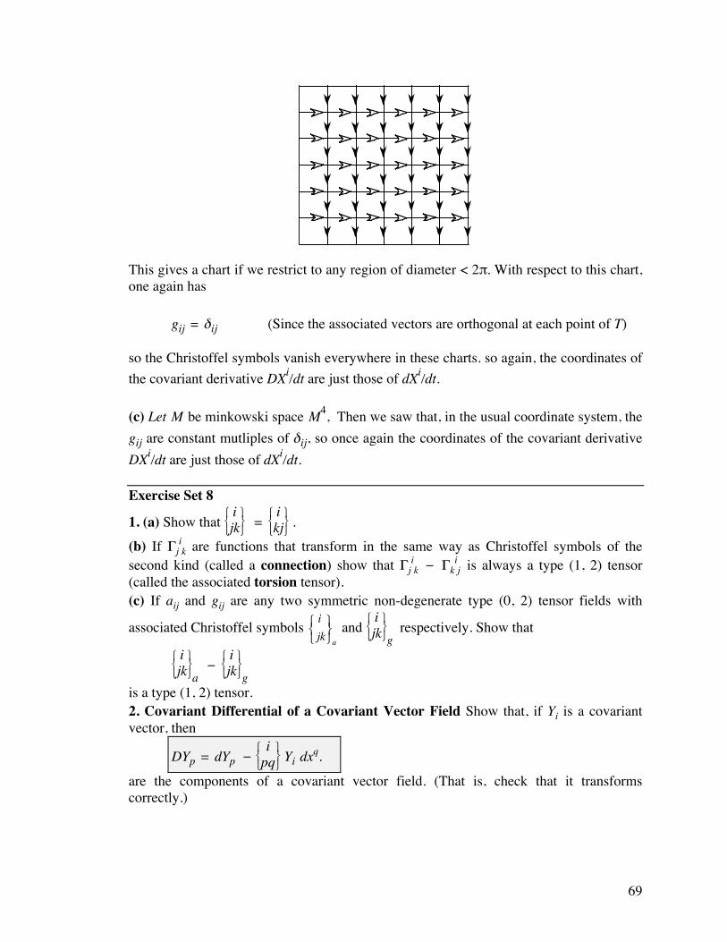
69

This gives a chart if we restrict to any region of diameter < 2π. With respect to this chart, one again has gij = ©ij (Since the associated vectors are orthogonal at each point of T) so the Christoffel symbols vanish everywhere in these charts. so again, the coordinates of the covariant derivative DXi/dt are just those of dXi/dt. (c) Let M be minkowski space M4, Then we saw that, in the usual coordinate system, the gij are constant mutliples of ©ij, so once again the coordinates of the covariant derivative DXi/dt are just those of dXi/dt. Exercise Set 8

1. (a) Show that ⎩⎨⎧

⎭⎬⎫i

jk = ⎩⎨⎧

⎭⎬⎫i

kj .

(b) If ¶jik are functions that transform in the same way as Christoffel symbols of the

second kind (called a connection) show that ¶jik - ¶k

ij is always a type (1, 2) tensor

(called the associated torsion tensor). (c) If aij and gij are any two symmetric non-degenerate type (0, 2) tensor fields with

associated Christoffel symbols ijk

! " #

$ % & a

and ⎩⎨⎧

⎭⎬⎫i

jk g respectively. Show that

⎩⎨⎧

⎭⎬⎫i

jk a -

⎩⎨⎧

⎭⎬⎫i

jk g

is a type (1, 2) tensor. 2. Covariant Differential of a Covariant Vector Field Show that, if Yi is a covariant vector, then

DYp = dYp - ⎩⎨⎧

⎭⎬⎫i

pq Yi dxq.

are the components of a covariant vector field. (That is, check that it transforms correctly.)

70

3. Covariant Differential of a Tensor Field Show that, it we define

DThp = dTh

p + ⎩⎨⎧

⎭⎬⎫h

rq Trp dxq -

⎩⎨⎧

⎭⎬⎫i

pq Thi dxq.

then the coordinates transform like a (1, 1) tensor. 4. Obtain the transformation equations for Chritstoffel symbols of the first and second kind. (You might wish to consult an earlier printing of these notes or the Internet site...) 5. Show directly that the coordinates of DXp/dt transform as a contravariant vector. 6. Show that, if Xi is any vector field on En, then its ordinary partial derivatives agree with Xp

|k. 7. Show that, if Xi and Yj are any two (contravariant) vector fields on M, then (Xi + Yi)|k = Xi

|k + Yi|k

(XiYj)|k = Xi|kY

j + XiYj|k.

8. Show that, if C is a path on M, then

DXi

dt = Xi|kdxk

dt . 9. Show that, if X and Y are vector fields, then

ddt “X, Y‘ = “

DXdt , Y‘ + “X,

DYdt ‘,

where the big D's denote covariant differentiation. 10. (a) What is ˙

|i if ˙ is a scalar field?

(b) Give a definition of the “contravariant” derivative, Xa|b of Xa with respect to xb, and show that Xa|b = 0 if and only if Xa

|b = 0.

71

9. Geodesics and Local Inertial Frames Let us now apply some of this theory to curves on manifolds. If a non-null curve C on M is parameterized by xi(t), then, as we saw in §6, we can reparameterize the curve using arc length,

s(t) = ⌡⎮⌠

a

t

±gijdxi

dudxj

du du,

(starting at some arbitrary point) as the parameter. The reason for wanting to do this is that the tangent vector Ti = dxi/ds is then a unit vector in the sense that ||T||2 = ±1 (see 6.5). If we were talking about a curve in E3, then the derivative of the unit tangent vector (again with respect to s is normal to the curve, and its magnitude is a measure of how fast the curve is “turning,” and so we call the derivative of Ti the curvature of C. If C happens to be on a manifold, then the unit tangent vector is still

Ti = dxi

ds = dxi

dt / dsdt = dxi/dt

±gpqdxp

dtdxq

dt

(the last formula is there if you want to actually compute it). But, to get the curvature, we need to take the covariant derivative:

Pi = DTi

ds

= D(dxi/ds)

ds

= d2xi

ds2 + ⎩⎨⎧

⎭⎬⎫i

pq dxp

ds dxq

ds

Definitions 9.1 The first curvature vector P of the curve C is

Pi = d2xi

ds2 + ⎩⎨⎧

⎭⎬⎫i

pq dxp

ds dxq

ds

A curve on M whose first curvature is zero is called a geodesic. Thus, a geodesic is a curve that satisfies the system of second order differential equations

72

d2xi

ds2 + ⎩⎨⎧

⎭⎬⎫i

pq dxp

ds dxq

ds = 0 Geodesic Equation

In terms of the parameter t, this becomes (see the exercises)

d2xi

dt2 dsdt -

dxi

dt d2sdt2

+ ⎩⎨⎧

⎭⎬⎫i

pq dxp

dt dxq

dt dsdt = 0,

where

dsdt = ±gij

dxi

dtdxj

dt . It can be shown using the calculus of variations that geodesics give us extremals of the length

L = ⌡⎮⌠

a

b

±gijdxi

dudxj

du du,

of a path from t = a to t = b. Note that P is a tangent vector at right angles to the curve C which measures its change relative to M. Question Why is P at right angles to C? Answer This can be checked as follows:

dds “T, T‘ = “

DTds , T‘ + “T,

DTds ‘ (Exercise Set 8 #9)

= 2“DTds , T‘ (symmetry of the scalar product)

= 2“P, T‘ (definition of P)

so that “P, T‘ = 12 dds “T, T‘.

But “T, T‘ = ±1 (refer back to the Proof of 6.5 to check this)

whence “P, T‘ = 12 dds (±1) = 0,

as asserted. Local Flatness, or “Local Inertial Frames” In various examples we looked at in the preceding section, all the Christoffel symbols

73

vanished in the eyes of certain charts, begging the: Question Can we find a chart (local coordinate system) such that the Christoffel symbols vanish—at least in the domain of that chart? Answer This is asking too much; we shall see later that the derivatives of the Christoffel symbols give an invariant tensor (called the curvature) which does not vanish in general (and on spheres in particular). This can be illustrated roughly on the 2-sphere: Suppose p is a point on the sphere (take the north pole for instance) and draw a small circle with center p and hence get four right-angled triangles with a common vertex. These triangles cannot be flattened (since the angles have to add up to π in a flat triangle). However, we do have the following. Proposition 9.2 (Existence of a Local Inertial Frame) If m is any point in the Riemannian manifold M, then there exists a local coordinate system xi at m such that:

(a) gij(m) = ⎩⎪⎨⎪⎧±1 if j = i

0 if j ≠ i = ±©ij

(b) ∂gij

∂xk(m) = 0

We call such a coordinate system a local inertial frame or a normal frame. (It follows that ¶i

jk(m) = 0.) Note that, if M is locally Minkowskian, then local intertial

frames are automatically Lorentz frames to first order. This is, mathematically, what physicists mean when they say that “spacetime is locally flat.” Before proving the proposition, we need a lemma. Lemma 9.3 (Some Equivalent Things) Let m é M. Then the following are equivalent: (a) g

pq,r(m) = 0 for all p, q, r.

(b) [pq, r]m = 0 for all p, q, r.

(c) ⎩⎨⎧

⎭⎬⎫r

pq m = 0 for all p, q, r.

Proof (a) ⇒ (b) follows from the definition of Christoffel symbols of the first kind. (b) ⇒ (a) follows from the identity g

pq,r = [qr, p] + [rp, q] (Check it!)

(b) ⇒ (c) follows from the definition of Christoffel symbols of the second kind.

74

(c) ⇒ (b) follows from the inverse identity

[pq, s] = gsr⎩⎨⎧

⎭⎬⎫r

pq . z Proof of Proposition 9.2‡ To start the proof, fix any chart xi near m with xi(m) = 0 for all i. Then recall from Section 6 that, if P is an invertible n×n matrix that diagonalizes G at the point m; PGPT = diag (±1, ±1, ..., ±1) then the change of coordinates defined by

xi = x–jPji gives us G— = diag (±1, ±1, ..., ±1) satisfying part (a). Before showing part (b), we make the following observation: Observation If we adjust the above change-of-coordinates and instead use xi = x–jPji

+ 12 x–jx–kB(i,j,k) (1)

then x–i = 0 for all i implies xi = 0 for all i, amd at the point specified by x–i = 0 one sees

from Taylor's theorem that Pji = ⎝⎜⎛

⎠⎟⎞∂xi

∂x–j

m and B(i,j,k) =

⎝⎜⎛

⎠⎟⎞∂2xi

∂x–j∂x–k

m . Since P is invertible,

it follows that, near this point, we can also invert the functions xi, giving us the desired change of coordinates x–i in terms of the xi, and also showing that m corresponds to x–i = 0, and that G— = diag (±1, ±1, ..., ±1) regardless of the choice of the B(i, j, k) (because G— depends only on the first derivatives). The functions x–i = x–i(xj) will be specified by constructing their inverses xi = xi(x–j) using a quadratic expression of the form (1). For part (b), we want to kill the partial derivatives ∂g–ij/∂x–

a by choosing appropriate values for the B(i, j, k) (that is, the second-order partial derivatives ∂2xi/∂x–j∂x–k). By the lemma, it suffices to arrange that

⎩⎨⎧

⎭⎬⎫p

hk (m) = 0.

‡ This is my own version of the proof. There is a version in Bernard Schutz's book, but the proof there

75

But ⎩⎨⎧

⎭⎬⎫p

hk (m) = ⎝⎜⎛

⎠⎟⎞

⎩⎨⎧

⎭⎬⎫t

ri ∂x–p

∂xt ∂xr

∂x–h ∂xi

∂x–k +

∂x–p

∂xt ∂2xt

∂x–h∂x–k(m)

= ∂x–p

∂xt ⎝⎜⎛

⎠⎟⎞

⎩⎨⎧

⎭⎬⎫t

ri ∂xr

∂x–h ∂xi

∂x–k +

∂2xt

∂x–h∂x–k (m)

so it suffices to arrange that

∂2xt

∂x–h∂x–k (m) = -

⎩⎨⎧

⎭⎬⎫t

ri ∂xr

∂x–h ∂xi

∂x–k (m) = -

⎩⎨⎧

⎭⎬⎫t

ri V(h)rV(k)i

That is, all we need to do is to define

B(t, h, k) = -⎩⎨⎧

⎭⎬⎫t

ri V(h)rV(k)i and we are done. ◆ Corollary 9.4 (Partial Derivatives Look Nice in Inertial Frames) Given any point m é M, there exist local coordinates such that

Xp|k(m) =

⎝⎜⎛

⎠⎟⎞∂Xp

∂xk m

Also, the coordinates of ⎝⎜⎛

⎠⎟⎞∂Xp

∂xk m in an inertial frame transform to those of Xp

|k(m) in

every frame. Corollary 9.5 (Geodesics are Locally Straight in Inertial Frames) If C is a geodesic passing through m é M, then, in any inertial frame, it has zero classical curvature at m (that is, d2xi/ds2 = 0). This is the reason we call them “inertial” frames: freely falling particles fall in straight lines in such frames (that is, with zero curvature, at least near the origin). Question Is there a local coordinate system such that all geodesics are in fact straight lines? Answer Not in general; if you make some geodesics straight, then others wind up curved. It is the curvature tensor that is responsible for this. This involves the derivatives of the Christoffel symbols, and we can't make it vanish.

76

Question If I throw a ball in the air, then the path is curved and also a geodesic. Does this mean that our earthly coordinates are not inertial? Answer Yes. At each instant in time, we can construct a local inertial frame corresponding to that event. But this frame varies from point to point along our world line if our world line is not a geodesic (more about this below), and the only way our world line can be a geodesic is if we were freely falling (and therefore felt no gravity). Technically speaking, the “earthly” coordinates we use constitute a momentary comoving reference frame; it is inertial at each point along our world line, but the directions of the axes are constantly changing in space-time. Here is an illustration in one (spacial) dimension:

Throwing up a Ball from an Accelerating frame in a 1-D World

z

t

z = ct

BallYou

z

t

t

z

zt

tz

P

Q R

Since the ball is moving freely, its world line is a geodesic (one of the principles of general relativity as we shall see later). The lines z = ±ct are the paths of photons going off in opposite directions. Since you are accelerating toward light speed, your world line is curved. It starts off vertical, since in your local coordinate system at the event P you are stationary, and z and t are in fact your local coordinates. As you move up the curve and recalibrate your coordinate axes, your time axis is always tangential to your world line (since you perceive yourself to be stationary, so dz–/dt– = slope of tangent (with the usual conventions reversed) = 0 along your world line at each point. The requirement that the z- and t-axes must be orthogonal with respect to the diagonal metric results in the narrowing of the angle between them. Some interesting events: P: The event that the ball leaves your hand. Its slope gives its initial velocity as you perceive it. Q: The ball comes back down (and continues to fall. R: Your velocity (in the original frame) is approaching light speed, so your world line becomes almost parallel to the photon's world line.

77

By moving these sets of z– and t--axes to the origin corresponds to not resetting your clock to zero at each instant. (We shall see later that your locally measured time is just the proper time † = s/c. In the resulting picture, we see your axes rotating “scissor-style” in spacetime.) Proposition 9.6 (Changing Inertial Frames) If x and x– are inertial frames at m é M, then, recalling that D is the matrix whose ij th entry is (∂xi/∂x–j), one has det D = det D— = ±1 Proof By definition of inertial frames,

gij(m) = ⎩⎪⎨⎪⎧±1 if j = i

0 if j ≠ i = ±©ij

and similarly for g–ij, so that g–ij = ±gij, whence det(g**) = ± det(g–**) = ±1. On the other hand,

g–ij = ∂xk

∂x–i ∂xl

∂x–j gkl,

which, in matrix form, becomes g–** = DTg**D. Taking determinants gives det(g–**) = det(DT) det(g**) det(D) = det(D)2 det(g**), giving ±1 = ±det(D)2, which must mean that det(D)2 = +1, so that det(D) = ±1 as claimed. ❆ Preferred Direction of the Time Axis Question Suppose that a particle travels along a (timelike) world line xi = xi(t) in locally Minkowskian space. Is there a “preferred” direction for the 4th axis V(4) in a “nice” locally inertial frame at some point p on the line? Answer We shall see later (proof of Proposition 11.3) we can choose such a frame by specifying V(4) as any timelike vector. So let us settle on V(4) = dxi/ds, the unit tangent vector, as our time coordinate.

78

Question Why? Answer In a “nice” frame, we want the origin to appear stationary; that is

⎣⎢⎡

⎦⎥⎤dxi

dx4 j

= 0 (j = 1, 2, 3) Spatial coordinates must be zero

Since dx4/ds ≠ 0 for all timelike paths, it follows from the chain rule that

⎣⎢⎡

⎦⎥⎤dxi

ds j

= 0 (j = 1, 2, 3). But we also know that ||dxi/ds||2 = ±1, meaning that, in this inertial frame that

⎣⎢⎡

⎦⎥⎤dxi

ds 4

= ± 1c

so that (recalling that proper time † = s/c), we have

⎣⎢⎡

⎦⎥⎤dxi

d† 4

= c⎣⎢⎡

⎦⎥⎤dxi

ds 4

= ±1

But this means that dxi/d† has coordinates (0, 0, 0, ±1) in our frame, so it equals ±V(4) =

±∂/∂x4. If we want the time axis to go in the direction of increasing proper time, we choose the (+) sign. Hence, the time axis must be dxi/d† in any Lorentz frame which appears stationary in the eyes of the observer moving along the world line xi(s). Notes (1) The above theorem also works if, in locally Minkowskian space, we use units in which det g = -c2 as in Lorentz frames. (2) If M is locally Minkowskian, then we usually choose V(4) as timelike, the other three V(1), V(2) and V(3) must be spacelike. (3) An annoying thing about the locally inertial frames we constructed is that the time coordinate is zero at the point m. if we are moving on a world line C, in locally Minkowskian space, we might prefer that, at each moment we decide to use a coordinate system, we do not need to set our clocks to midnight (t = 0). So instead we can fix a point t = t0 on C as “midnight” and then change our inertial frame (xi, x2, x3, x4) by defining

x–i = ⎩⎪⎨⎪⎧x

i if i ≠ 4

x4 + † if i = 4

79

where s is arc length from the point t = t0 and † = s/c is proper time. Note that the new frame is still locally inertial (why?), so we can think of the world line as a curved “time axis”. Oriented Manifolds and the Volume Form Definition 9.7 Two (not necessarily inertial) frames x and x– have the same parity if det D— > 0. M is orientable if it has an atlas all of whose charts have the same parity. Two such atlases are equivalent if the charts in one have the same parity as the charts in the other. Notice that, given any two atlases, either they are equivalent, or can be made so if we take one of these atlases and reverse the direction of one of the axes in each of its charts. This means there are really two sets of equivalence classes of atlases: those that fit in with a chosen one, and those that need an axis reversed. An orientation of M is then a choice of one or other of these classes. An oriented manifold is a manifold equipped with an orientation. Notes 1. Reversing the direction of any one of the axes in a chart reverses its orientation. 2. If M is an oriented manifold and m é M, then we can choose an oriented inertial frame x– at m, so that the change-of-coordinates matrix D in the proof of Proposition 9.2 has positive determinant. Further, if D happens to be the change-of-coordinates from one oriented inertial frame to another, then det(D) = +1. 3. E

3 has two orientations: one given by any left-handed system, and the other given by

any right-handed system. 4. In the homework, you will see that spheres are orientable, whereas Klein bottles are not. We now show how we can use inertial frames to construct a tensor field. Definition 9.8 Let M be an oriented n-dimensional Riemannian manifold. The Levi-Civita tensor œ of type (0, n) or volume form is defined as follows. If x– is any coordinate system and m é M, then define œ–i1i2…in

(m) = det (Di1 Di2

… Din )

= determinant of D with columns permuted according to the indices where Dj is the j th column of the change-of-coordinates matrix ∂xk/∂x–l, and where x is any oriented inertial frame at m.†† In the homework, you will show that, in every frame x, the tensor is given by

†† Note that this tensor cannot be defined without a metric being present. In the absence of a metric, the best you can do is define a “relative tensor,” which is not quite the same, and what Rund calls the “Levi-Civita symbols” in his book. Wheeler, et al. just define it for Minkowski space. Carroll defines it a little differently, but his definition is equivalent to ours.

80

œi1i2…in

= ±det g ß(i1, i2, ... in) where

ß(i1, i2, ... in) = ⎩⎪⎨⎪⎧1 if (i1, i2, … , in) is an even permutation of (1, 2, … , n)

-1 if if (i1, i2, … , in) is an odd permutation of (1, 2, … , n)

Note œ is a completely antisymmetric tensor. If x– is itself an inertial frame, then, since det(D) = +1 (see Note 2 above) the coordinates of œ(m) are given by

œ–i1i2…in (m) = ß(i1, i2, ... in).

(Compare this with the metric tensor, which is also “nice” in inertial frames.) Proposition 9.9 (Levi-Civita Tensor) The Levi-Civita tensor is a well-defined, smooth tensor field. Proof To show that it is well-defined, we must show independence of the choice of inertial frames. But, if œ and µ are defined at m é M as above by using two different inertial frames, with corresponding change-of-coordinates matrices D and E, then D—E is the change-of coordinates from one inertial frame to another, and therefore has determinant 1. Now, œ–i1i2…in

(m) = det (Di1 Di2

… Din )

= det D E–i1i2…in

(where E–i1i2…in is the identity matrix with columns ordered as shown in the indices)

= det DD—E E–i1i2…in

(since D—E has determinant 1; this being where we use the fact that things are oriented!) = det E E–i1i2…in

= µ–i1i2…in ,

showing it is well-defined at each point. We now show that it is a tensor. If x– and y– are any two oriented coordinate systems at m and change-of-coordinate matrices D and E with respect to some inertial frame x at m, and if the coordinates of the tensor with respect to these coordinates are œ–k1k2…kn

and µ–r1r2…rn = det (Er1

Er2 … Ern

) respectively, then at the point m, œ–k1k2…kn

= det (Dk1 Dk2

… Dkn )

= œi1i2…in ∂xi1

∂x–k1 ∂xi2

∂x–k2 … ∂x

in

∂x–kn

81

(by definition of the determinant! since œi1i2…in is just the sign of the

permutation!)

= œi1i2…in ∂xi1

∂y–r1 ∂xi2

∂y–r2 … ∂x

in

∂y–rn ∂y–r1

∂x–k1 ∂y–r2

∂x–k2 … ∂y–

rn

∂x–kn

= µ–r1r2…rn ∂y–r1

∂x–k1 ∂y–r2

∂x–k2 … ∂y–

rn

∂x–kn ,

showing that the tensor transforms correctly. Finally, we assert that det (Dk1

Dk2 … Dkn

) is a smooth function of the point m. This depends on the change-of-coordinate matrices to the inertial coordinates. But we saw that we could construct inertial frames by setting

⎝⎜⎛

⎠⎟⎞∂xi

∂x–j

m = V(j)i,

where the V(j) were an orthogonal base of the tangent space at m. Since we can vary the coordinates of this base smoothly, the smoothness follows. ❄ Example 9.10 In E3, the Levi-Civita tensor coincides with the totally antisymmetric third-order tensor œijk in Exercise Set 5. In the Exercises, we see how to use it to generalize the cross-product. Exercise Set 9 1. Derive the equations for a geodesic with respect to the parameter t. 2. Obtain an analogue of Corollary 8.3 for the covariant partial derivatives of type (2, 0) tensors. 3. Use inertial frames argument to prove that gab|c = gab

|c = 0. (Also see Exercise Set 4 #1.) 4. Show that, if the columns of a matrix D are orthonormal, then det D = ±1. 5. (a) Prove that, in every frame x, the Levi-Civita tensor is given by œi1i2…in

= ±det G ß(i1, i2, ... in) where

ß(i1, i2, ... in) = ⎩⎪⎨⎪⎧1 if (i1, i2, … , in) is an even permutation of (1, 2, … , n)

-1 if if (i1, i2, … , in) is an odd permutation of (1, 2, … , n)

[Hint: If Ak is the kth column of any square matrix A, then det(Ai1

, Ai2, ..., Ain

) = ß(i1, i2, ... in) det A.] (b) Deduce that, if œ is the Levi-Civita tensor, then, in any frame, œi1i2…in

= 0 whenever two of the indices are equal. Thus, the only non-zero coordinates occur when all the indices differ.

6. Use the Levi-Civita tensor to show that, if x is any inertial frame at m, and if X(1), . . . , X(n) are any n contravariant vectors at m, then

82

det “X(1)| . . . |X(n)‘ is a scalar. 7. The Volume 1-Form (A Generalization of the Cross Product) If we are given n-1 vector fields X(2), X(3), . . . , X(n) on the n-manifold M, define a covariant vector field by (X(2)…X(3)………X(n))j = œj i2…in

X(2)i2 X(3)i3 … X(n)in , where œ is the Levi-Civita tensor. Show that, in any inertial frame at a point m on a Riemannian 4-manifold, ||X(2)…X(3)…X(4)||2 evaluated at the point m, coincides, up to sign, with the square of the usual volume of the three-dimensional parallelepiped spanned by these vectors by justifying the following facts. (a) Restricting your attention to Riemannian 4-manifolds, let A, B, and C be vectors at m, and suppose—as you may—that you have chosen an inertial frame at m with the property that A1 = B1 = C1 = 0. (Think about why you can you do this.) Show that, in this frame, A…B…C has only one nonzero coordinate: the first. (b) Show that, if we consider A, B and C as 3-vectors a , b and c respectively by ignoring their first (zero) coordinate, then (A…B…C)1 = a.(b¿c), which we know to be ± the volume of the parallelepiped spanned by a , b and c . (c) Defining ||C||2 = CiCjg

ij (recall that gij is the inverse of gkl), deduce that the scalar ||A…B…C||2 is numerically equal to square of the volume of the parallelepiped spanned by the vectors a , b and c . (Note also that ||A…B…C||2, being a scalar, does not depend on the choice of coordinate system—we always get the same answer, no matter what coordinate system we choose.) 8. Define the Levi-Civita tensor of type (n, 0) , and show that

œi1i2…in œj1j2…jn =

⎩⎪⎨⎪⎧1 if (i1, … , in) is an even permutation of (j1, … , jn)

-1 if (i1, … , in) is an odd permutation of (j1, … , jn) .

83

10. The Riemann Curvature Tensor First, we need to know how to translate a vector along a curve C. Let Xj be a vector field. We have seen that a parallel vector field of constant length on M must satisfy

DXj

dt = 0 ……… (I) for any path C in M. Definition 10.1 The vector field Xj is parallel along the curve C if it satisfies

DXj

dt = dXj

dt + ¶ijh X

i dxh

dt = 0,

for the specific curve C, where we are writing the Christoffel symbols ⎩⎨⎧

⎭⎬⎫j

ih as ¶ijh. This

notion is independent of the paramaterization of C (see the exercises). If Xj is parallel along C, which has parameterization with domain [a, b] and corresponding points å and ∫ on M, then, since

dXj

dt = -¶ijh X

i dxh

dt ……… (I) we can integrate to obtain

Xj(∫) = Xj(å) - ⌡⎮⌠

a

b

¶ijh X

i dxh

dt dt ……… (II)

Question Given a fixed vector Xj(å) at the point å é M, and a curve C originating at å, it is possible to define a vector field along C by transporting the vector along C in a parallel fashion? Answer Yes. Notice that the formula (II) is no good for this, since the integral already requires Xj to be defined along the curve before we start. But we can go back to (I), which is a system of first order linear differential equations. Such a system always has a unique solution with given initial conditions specified by Xj(å). Note however that it gives Xj as a function of the parameter t, and not necessarily as a well-defined function of position on M. In other words, the parallel transport of X at p é M depends on the path to p. (See the figure.) If it does not, then we have a parallelizable manifold.

84

Definition 10.2 If Xj(å) is any vector at the point å é M, and if C is any path from å to ∫ in M, then the parallel transport of Xj(å) along C is the vector Xj(∫) given by the solution to the system (I) with initial conditions given by Xj(å). Examples 10.3 (a) Let M = T. Then we saw that there is an atlas of charts under each of which the Christoffel symbols vanish completely. So (I) above becomes dXi/dt = 0, which we can solve by using the constant vector Xj at each point in a chart. (Uniqueness shows that this is what we must do.) This procedure also shows that the entire torus T is parallelizable (the procedure does not depend on the path we choose). (b) Let M = En or M4. then the arguments of part (a) apply to show that these are parallelizable. (c) If C is a geodesic in M given by xi = xi(s), where we are using arc-length s as the parameter (see Exercise Set 8 #1) then the vector field dxi/ds is parallel along C. (Note that this field is only defined along C, but (I) still makes sense.) Why? because

D(dxj/ds)

Ds = d2xj

ds2 + ¶ijh dxi

ds dxh

ds ,

which must be zero for a geodesic. (d) Proper Coordinates in Relativity Along Geodesics According to relativity, we live in a Riemannian 4-manifold M, but not the flat Minkowski space. Further, the metric in M has signature (1, 1, 1, -1). Suppose C is a geodesic in M given by xi = xi(t), satisfying the property

“ dxi

dt , dxi

dt ‘ < 0.

Recall that we refer to such a geodesic as timelike. Looking at the discussion before Definition 7.1, we see that this corresponds, in Minkowski space, to a particle traveling at sub-light speed. It follows that we can choose an orthonormal basis of vectors {V(1),

85

V(2), V(3), V(4)} of the tangent space at m with the property given in the proof of 9.2, with V(4) = dxi/ds (actually, it is dxi/d† instead if our units have c ≠ 1). We think of V(4) as the unit vector in the direction of time, and V(1), V(2) and V(3) as the spatial basis vectors. Using parallel translation, we obtain a similar set of vectors at each point along the path. (The fact that the curve is a geodesic guarantees that parallel translation of the time axis will remain parallel to the curve.) Finally, we can use the construction in 9.2 to flesh these frames out to full coordinate systems defined along the path. (Just having a set of orthogonal vectors in a manifold does not give a unique coordinate system, so we choose the unique local inertial one there, because in the eyes of the observer, spacetime should be flat.) Question Does parallel transport preserve the relationship of these vectors to the curve. That is, does the vector V(4) remain parallel, and do the vectors {V(1), V(2), V(3), V(4)} remain orthogonal in the sense of 9.2? Answer If X and Y are vector fields, then

ddt “X, Y‘ = “

DXdt , Y‘ + “X,

DYdt ‘,

where the big D's denote covariant differentiation. (Exercise Set 8 #9). But, since the terms on the right vanish for fields that have been parallel transported, we see that “X, Y‘ is independent of t, which means that orthogonal vectors remain orthogonal and that all the directions and magnitudes are preserved, as claimed. Note At each point on the curve, we have a different coordinate system! All this means is that we have a huge collection of charts in our atlas; one corresponding to each point on the path. This (moving) coordinate system is called the momentary comoving frame of reference and corresponds to the “real life” coordinate systems. (e) Proper Coordinates in Relativity Along Non-Geodesics If the curve is not a geodesic, then parallel transport of a tangent vector need no longer be tangent. Thus, we cannot simply parallel translate the coordinate axes along the world line to obtain new ones, since the resulting frame may not be stationary in the eyes of the observer moving along the given world line (see the discussion in the previous section). We shall see in Section 11 how to correct for that when we construct our comoving reference frames. Question Under what conditions is parallel transport independent of the path? If this were the case, then we could use formula (I) to create a whole parallel vector field of constant length on M, since then DXj/dt = 0.

86

Answer To answer this question, let us experiment a little with a fixed vector V = Xj(a) by parallel translating it around a loop C in the x1x2-plane. Since parallel transport is independent of the path, we get 0 for the path integral around C.:

-⌡⎮⌠

a

b

¶ijh X

i dxh

dt dt = 0

(We are retaining the minus sign becuase of equation (II) above, although it is not necesary, of course.) Because xh is independent of t unless h = 1, 2, the corresponding terms dxh/dt vanish, and this integral boils down to

-⌡⎮⌠

a

b

¶ij1 X

i dx1

dt + ¶ij2 X

i dx2

dt dt = 0

Notice that this is just a two-dimensional path integral of the vector field “P, Q‘ = “ ¶i

j1 X

i, ¶ij2 X

i ‘. By Green's theorem, the path integral is equal to

-⌡⎮⌠ ⌡⎮⌠

R

⎣⎢⎡

⎦⎥⎤∂Q

∂x1 - ∂P∂x2 dA =

⌡⎮⌠ ⌡⎮⌠

R

⎣⎢⎡

⎦⎥⎤∂

∂x2( )¶ij1 X

i - ∂∂x1( )¶i

j2 X

i ,

which must therefore vanish. For this integral to vanish for every closed path in the x1x2-

plane, the integrand ⎣⎢⎡

⎦⎥⎤∂

∂x2( )¶ij1 X

i - ∂∂x1( )¶i

j2 X

i has to vanish everywhere.

To analyze this expression, we first use the product rule, getting

⎣⎢⎡

⎦⎥⎤Xi

∂∂x2¶i

j1 + ¶i

j1∂∂x2 X

i - Xi ∂∂x1¶i

j2 - ¶i

j2∂∂x1 X

i ……… (III)

Next, we recall the "chain rule" formula

DXj

dt = Xj|hdxh

dt in the homework. Since the term on the left must be zero along the closed path (definition of parallel transport being independent of the path) we see that (I) is equivalent to saying that the partial derivatives Xj

|h = 0

87

for every index p and k (and along the relevant path segment)* since the terms dxh/dt are in general non-zero. By definition of the partial derivatives Xj

|h, this means that

∂Xj

∂xh + ¶ijhX

i = 0,

so that

∂Xj

∂xh = - ¶ijhX

i.

We now substitute these expressions in (III) to obtain

⎣⎢⎡

⎦⎥⎤Xi

∂∂x2¶i

j1 - ¶i

j1¶p

i2X

p - Xi ∂∂x1¶i

j2 + ¶i

j2¶p

i1X

p = 0

Now change the dummy indices in the first and third terms and obtain

⎣⎢⎡

⎦⎥⎤∂

∂x2¶pj1 - ¶i

j1¶p

i2-

∂∂x1¶p

j2 + ¶i

j2¶p

i1 Xp = 0

This formula has the form

Rpj12X

p = 0 ………… (IV)

(indices borrowed from the Christoffel symbol in the first term, with the extra index from the x in the denominator) where the quantity Rp

j12 is known as the curvature tensor.

Curvature Tensor

Rbacd =

⎣⎢⎡

⎦⎥⎤

¶bic¶i

ad - ¶b

id¶i

ac +

∂¶bac

∂xd - ∂¶b

ad

∂xc

The terms are rearranged (and the Christoffel symbols switched) so you can see the index pattern, and also that the curvature is antisymmetric in the last two covariant indices.

* Notice that we are taking partial derivatives in the direction of the path, so that they do make sense for this curious field that is only defined along the square path!

88

Rbacd = - Rb

adc

The fact that it is a tensor follows from the homework. As out choice of the vector field X is arbitrary, it must follow from (IV) that Rp

j12 = 0 for

parallel transport to be independent of the path for arbitrary vector fields X. Finally, since out choices of indices 1 and 2 were arbitrary, we see the following. Proposition 10.4 (Curvature and Parallel Transport) Assume M is simply connected. A necessary and sufficient condition that parallel transport be independent of the path is that the curvature tensor vanishes. Definition 10.5 A manifold with zero curvature is called flat. Properties of the Curvature Tensor We first obtain a more explicit description of Rb

acd

in terms of the partial derivatives of the gij. First, introduce the notation

gij,k = ∂gij

∂xk

for partial derivatives, and remember that these are not tensors. Then, the Christoffel symbols and curvature tensor are given in the convenient form

¶bac =

12 gak(gck,b + gkb,c - gbc,k)

Rb

acd = [¶b

ic¶i

ad - ¶b

id¶i

ac + ¶b

ac,d - ¶b

ad,c].

We can lower the index by defining

Rabcd = gbiRaicd

Substituting the first of the above (boxed) formulas into the second, and using symmetry of the second derivatives and the metric tensor, we find (exercise set)

Covariant Curvature Tensor in Terms of the Metric Tensor Rabcd =

12 (gbc,ad - gbd,ac + gad,bc - gac,bd) + ¶a

jd¶bjc - ¶a

jc¶bjd

(We can remember this by breaking the indices a, b, c, d into pairs other than ab, cd (we can do this two ways) the pairs with a and d together are positive, the others negative.) Notes 1. We have snuck in new kinds of Christoffel symbols ¶ijk given by

89

¶ijk = gpj ¶i

pk.

2. Some symmetry properties: Rabcd = -Rabdc = -Rbacd and R

abcd = R

cdab (see the

exercise set) 3. We can raise the index again by noting that gbiRaicd = gbigijRa

jcd = ©b

j Rajcd = Ra

bcb.

Now, let us evaluate some partial derivatives in an inertial frame (so that we can ignore the Christoffel symbols) cyclically permuting the last three indices as we go: Rabcd,e + Rabec,d + Rabde,c

= 12 (gad,bce - gac,bde + gbc,ade - gbd,ace

+ gac,bed - gae,bcd + gbe,acd - gbc,aed + gae,bdc - gad,bec + gbd,aec - gbe,adc) = 0 Now, I claim this is also true for the covariant partial derivatives:

Bianchi Identities Rabcd|e + Rabec|d + Rabde|c = 0

Indeed, let us evaluate the left-hand side at any point m é M. Choose an inertial frame at m. Then the left-hand side coincides with Rabcd,e + Rabec,d + Rabde,c, which we have shown to be zero. Now, since a tensor which is zero is some frame is zero in all frames, we get the result! Definitions 10.6 The Ricci tensor is defined by Rab = Ra

ibi = gijRajbi

we can raise the indices of any tensor in the usual way, getting Rab = gaigbjRij. In the exercise set, you will show that it is symmetric, and also (up to sign) is the only non-zero contraction of the curvature tensor. We also define the Ricci scalar, or Ricci curvature, or just curvature by R = gabRab = gabgcdRacbd

90

The last thing we will do in this section is play around with the Bianchi identities. Multiplying them by gbc: gbc[Rabcd|e + Rabec|d + Rabde|c] = 0 Since gij

|k = 0 (see Exercise Set 8), we can slip the gbc into the derivative, getting -Rad|e + Rae|d + Ra

cde|c = 0.

Contracting again gives gad[-Rad|e + Rae|d + Ra

cde|c] = 0,

or -R|e + Rd

e|d + Rdcde|c = 0,

or -R|e + Rd

e|d + Rce|c = 0.

Combining terms and switching the order now gives Rb

e|b - 12 R|e = 0,

or Rb

e|b - 12 ©b

e R|b = 0 Multiplying this by gae, we now get Rab

|b - 12 gabR|b = 0, (Rab is symmetric)

or Gab

|b = 0, where we make the following definition:

Einstein Tensor

Gab = Rab - 12 gabR

Einstein's field equation for a vacuum states that Gab = 0 (as we shall see later…).

91

Examples 10.7 (a) If M is any parallelizable manifold (like En or M4) then the curvature tensor vanished everywhere, so that in particular R = 0. (b) Take the 2-sphere of radius r with polar coordinates, where we saw that

g** = ⎣⎢⎡

⎦⎥⎤r2sin2˙ 0

0 r2 .

The coordinates of the covariant curvature tensor are given by Rabcd =

12 (gbc,ad - gbd,ac + gad,bc - gac,bd) + ¶a

jc¶jbd - ¶a

jd¶jbc.

Let us calculate Rø˙ø˙. (Note: when we use Greek letters, we are referring to specific terms, so there is no summation when the indices repeat!) So, a = c = ø, and b = d = ˙. (Incidentally, this is the same as R˙ø˙ø by the last exercise below.) The only non-vanishing second derivative of g** is gøø,˙˙ = 2r2(cos2˙ - sin2˙), giving

12 (g˙ø,ø˙ - g˙˙,øø + gø˙,˙ø - gøø,˙˙) = r2(sin2˙ - cos2˙).

The only non-vanishing first derivative of g** is gøø,˙ = 2r2sin ˙ cos ˙, giving ¶a

jc¶jbd = ¶ø

jø¶j˙˙ = 0,

since b = d = ˙ eliminates the second term (two of these indices need to be ø in order for the term not to vanish.)

¶ajd¶jbc = ¶ø

j˙¶j˙ø =

14 ⎝⎜⎛

⎠⎟⎞2 cos ˙

sin ˙ (-2r2sin ˙ cos ˙) = -r2cos2˙

Combining all these terms gives Rø˙ø˙ = r2(sin2˙ - cos2˙) + r2cos2˙ = r2sin2˙.

92

We now calculate Rab = gcdRacbd Røø = g˙˙Rø˙ø˙ = sin2˙ and R˙˙ = gøøR˙ø˙ø

= sin2˙sin2˙

= 1.

All other terms vanish, since g is diagonal and R**** is antisymmetric. This gives R = gabRab = gøøRøø + g˙˙R˙˙

= 1

r2sin2˙ (sin2˙) +

1r2 =

2r2 .

Summary of Some Properties of Curvature Etc. ¶

abc = ¶

cba ¶

abc = ¶

cba

Rabcd

= Rabdc

R

abcd = -R

bacd R

abcd = -R

abdc

R

abcd = R

cdab Note that a,b and c,d always go together

Rab = Raibi = gijRajbi

Rab

= Rba

R = gabR

ab = gacgbdR

abcd

Rab = gaiR

ib

Rab = gaigbjRij

Gab = Rab - 12 gabR

Exercise Set 10 1. Show that parallel transport along a curve C from point p to point q is independent of the paramaterization. 2. Derive the formula for the curvature tensor in terms of the gij. 3. (a) Show that the curvature tensor is antisymmetric in the last pair of variables: Rb

acd = - Rb

adc

93

(b) Use part (a) to show that the Ricci tensor is, up to sign, the only non-zero contraction of the curvature tensor. (c) Prove that the Ricci tensor is symmetric.

4. (cf. Rund, pp. 82-83) (a) Show that

Xj|h|k =

∂∂xk (X

j|h) + ¶m

jk(X

m|h) - ¶h

lk(X

j| l)

= ∂2Xj

∂xh∂xk + Xl ∂∂xk ¶l

jh +¶l

jh∂∂xkX

l + ¶mjk∂∂xhX

m + ¶mjk¶l

mhX

l - ¶hlk(X

j| l)

(b) Deduce that Xj

|h|k - Xj|k|h = Rl

jhkX

l - ShlkX

j| l = Rl

jhkX

l where Sh

lk = ¶h

lk - ¶k

lh = 0.

(c) Now deduce that the curvature tensor is indeed a type (1, 3) tensor. 5. Show that Rabcd is antisymmetric on the pairs (a, b) and (c, d). 6. Show that R

abcd = R

cdab by first checking the identity in an inertial frame.

7. Deduce from the fact that spheres of dimension greater than 1 have constant non-zero Ricci curvature everywhere the fact that no charts exist in which the Christoffel symbols vanish identically.

94

11. A Little More Relativity: Comoving Frames and Proper Time Recall the following from §6: Definition 11.1 A locally Minkowskian 4-manifold is a 4-manifold in which the metric has signature (1, 1, 1, -1) (eg., the world according to Einstein). By Proposition 9.2, if M is Minkowskian and m é M, then one can find a locally inertial frame at m such that the metric at m has the form diag(1, 1, 1, -1). We actually have some flexibility: we can, if we like, adjust the scaling of the x4-coordinate to make the metric look like diag(1, 1, 1, -c2). In that case, the last coordinate is the local time coordinate. Later, we shall convert to units of time in which c = 1, but for now, let us use this latter kind of inertial frame. Now let C be a timelike curve in the Minkowskian 4-manifold M. Definition 11.2 A momentary comoving reference frame for C (MCRF) associates to each point m é C a locally inertial frame whose last basis vector is parallel to the curve and in the direction of increasing parameter s. Further, we require the frame coordinates to vary smoothly with the parameter of the curve. (This can be made precise by talking about things called homotopies.) Proposition 11.3 (Existence of MCRF's) If C is any timelike curve in the Minkowskian 4-manifold M, then there exists an MCRF for C. Proof Fix p

0 é C and a Lorentz frame W(1), W(2), W(3), W(4) of Mp0

(so that

g**

= diag(1, 1, 1, -c2).) We want to change this set to a new Lorentz frame V(1), V(2),

V(3), V(4) with

V(4) = dxi

d† Recall that † = s/c So let us define V(4) as indicated. Then it is tangent to C at p

0. Further,

||V(4)||2 = ⎪⎪⎪

⎪⎪⎪

⎪⎪⎪

⎪⎪⎪dxi

d†

2

= ⎪⎪⎪

⎪⎪⎪

⎪⎪⎪

⎪⎪⎪dxi

ds

2

⎪⎪⎪

⎪⎪⎪ds

d†

2

= (-1)c2 = -c2. Intuitively, V(4) is the time axis for the observer at p

0: it points in the direction of

increasing proper time †. We can now flesh out this orthonormal set to obtain an inertial frame at p

0. For the other vectors, take

95

V(i) = W(i) + 2c2 “W(i), V(4)‘ V(4)

for i = 1, 2, 3.† Then

“V(i),V(j)‘ = “W(i),W(j)‘ + 4c2“W(i),W(4)‘ “W(j),W(4)‘ +

4c4“W(i),V(4)‘“W(j),V(4)‘

||V(4)||2 = 0 by orthogonality of the W's and the calculation of ||V(4)||2 above. Also,

“V(i),V(i)‘ = “W(i),W(i)‘ + 4c2“W(i),W(4)‘2 +

4c4“W(i),V(4)‘2 ||V(4)||2

= ||W(i)||2 = 1 so there is no need to adjust the lengths of the other axes. Call this adjustment a time shear. We can now use 9.2 to flesh this out to an inertial frame there (and also adjust the time coordinate to taste as in the remarks after 9.2). At another point p along the curve, proceed as follows. For V(4), again use dxi/d† (evaluated at p). For the other axes, start by talking W(1), W(2), and W(3) to be the parallel translates of the V(i) along C. These may not be orthogonal to V(4), although they are orthogonal to each other (since parallel translation preserves orthogonality). To fix this, use the same time shearing trick as above to obtain the V(i) at p. Note that the spatial coordinates have not changed in passing from W(i) to V(i)—all that is changed are the time-coordinates. Now again use 9.2 to flesh this out to an inertial frame.

path of the particle

x–4x–1

x–20m

By construction, the frame varies smoothly with the point on the curve, so we have a smooth set of coordinates.

† That this process will never give a zero vector (and therefore always works) is seen in the Exercise set.

96

The figure after Corollary 9.4 gives a nice illustration of the comoving frame of an accelerating observer in M4. Proposition 11.4 (Proper Time is Time in a MCRF) In a MCRF x–, the x4-coordinate (time) is proper time †. "Proof" First, we defined the time coordinate of every point as equal to the proper time of its world line starting at some specified event. To see that this is consistent with reality, note that, since dx–4/d† = 1 from what we know about the arc length parameter, it follows that the time coordinate x–4 is moving at a rate of one unit per unit of proper time †. Therefore, they must agree. A particular (and interesting) case of this is the following, for special relativity. Proposition 11.5 (In SR, Proper Time = Time in the Moving Frame) In SR, the proper time of a particle moving with a constant velocity v is the t-coordinate of the Lorentz frame moving with the particle. Proof

† = sc =

1c ⌡⎮⌠

-gijdxi

dtdxj

dt dt.

The curve C has parametrization (vt, 0, 0, t) (we are assuming here movement in the x1-direction), and g** = diag (1, 1, 1, -c2). Therefore, the above integral boils down to

† = 1c ⌡⌠ -(v2-c2) dt

= 1c ⌡⌠c 1-v2/c2 dt

= t 1-v2/c2 . But, by the (inverse) Lorentz transformations:

t = t– + vx–/c2

1-v2/c2 =

t–

1-v2/c2 , since x– = 0 for the particle.

Thus, t– = t 1-v2/c2 = †,

97

as required. Definition 11.6 Let C be the world line of a particle in a Minkowskian manifold M. Its four velocity is defined by

ui = dxi

d† .

Note By the proof of Proposition 11.3, we have

“u, u‘ = ⎪⎪⎪

⎪⎪⎪

⎪⎪⎪

⎪⎪⎪dxi

d† 2

= -c2. in all frames. In other words, four-velocity is timelike and of constant magnitude. Example 11.7 Four Velocity in SR Let us calculate the four-velocity of a particle moving with uniform velocity v with respect to some (Lorentz) coordinate system in Minkowski space M = E4. Thus, xi are the coordinates of the particle at proper time †. We need to calculate the partial derivatives dxi/d†, and we use the chain rule:

dxi

d† = dxi

dx4 dx4

d†

= vi dx4

d† for i = 1, 2, 3 since x4 is time in the unbarred system. Thus, we need to know dx4/d†. (In the barred system, this is just 1, but this is the unbarred system...) Since x–4 = †, we use the (inverse) Lorentz transformation:

x4 = x–4 + vx–1/c2

1 - v2/c2 ,

assuming for the moment that v = (v, 0, 0). However, in the frame of the particle, x–1 = 0, and x–4 = †, giving

x4 = †

1 - v2/c2 ,

and hence

dx4

d† = 1

1 - v2/c2 .

98

Now, using the more general boost transformations, we can show that this is true regardless of the direction of v if we replace v2 in the formula by (v1)2 + (v2)2 + (v3)2 (the square magnitude of v). Thus we find

ui = dxi

d† = vi dx4

d† = vi

1 - v2/c2 (i = 1, 2, 3)

and

u4 = dx4

d† = 1

1 - v2/c2 .

Hence the coordinates of four velocity in the unbarred system are given by

Four Velocity in SR u* = (v1, v2, v3, 1)/ 1-v2/c2

We can now calculate “u, u‘ directly as

“u, u‘ = u*

⎣⎢⎡

⎦⎥⎤1 0 0 0

0 1 0 00 0 1 00 0 0 -c2

uT

= v2-c2

1-v2/c2 = -c2.

Special Relativistic Dynamics If a contravariant “force” field F (such as an electromagnetic force) acts on a particle, then its motion behaves in accordance with

m0dud† = F ,

where m0 is a scalar the rest mass of the particle; its mass as measured in its rest (that is, comoving) frame. We use the four velocity to get four momentum, defined by pi = m0u

i. Its energy is given by the fourth coordinate, and is defined as

99

E = c2p4 = m0c

2

1-v2/c2 .

Note that, for small v,

E = m0(1-v2/c2)-1/2 ‡ m0c2 +

12 m0v

2. In the eyes of a the comoving frame, v = 0, so that E = m0c

2. This is called the rest energy of the particle, since it is the energy in a comoving frame. Definitions 11.7 If M is any locally Minkowskian 4-manifold and C is a timelike path or spacelike (thought of as the world line of a particle), we can define its four momentum as its four velocity times its rest mass, where the rest mass is the mass as measured in any MCRF. Exercise Set 11 1. What are the coordinates of four velocity in a comoving frame? Use the result to check that “u, u‘ = -c2 directly in an MCRF. 2. What can you say about “p, p‘, where p is the 4-momentum? 3. Is energy a scalar? Explain 4. Look up and obtain the classical Lorentz transformations for velocity. (We have kind of done it already.) 5. Look up and obtain the classical Lorentz transformations for mass. 6. Prove that V(*) as defined in Proposition 11.3 are never zero.

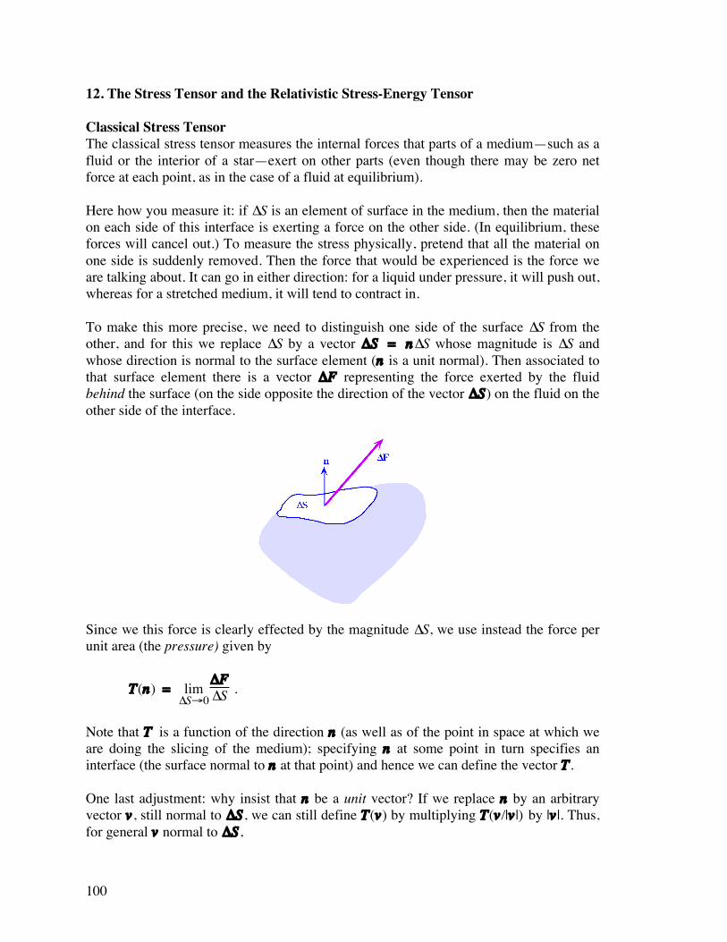
100

12. The Stress Tensor and the Relativistic Stress-Energy Tensor Classical Stress Tensor The classical stress tensor measures the internal forces that parts of a medium—such as a fluid or the interior of a star—exert on other parts (even though there may be zero net force at each point, as in the case of a fluid at equilibrium). Here how you measure it: if ∆S is an element of surface in the medium, then the material on each side of this interface is exerting a force on the other side. (In equilibrium, these forces will cancel out.) To measure the stress physically, pretend that all the material on one side is suddenly removed. Then the force that would be experienced is the force we are talking about. It can go in either direction: for a liquid under pressure, it will push out, whereas for a stretched medium, it will tend to contract in. To make this more precise, we need to distinguish one side of the surface ∆S from the other, and for this we replace ∆S by a vector ∆S = n∆S whose magnitude is ∆S and whose direction is normal to the surface element (n is a unit normal). Then associated to that surface element there is a vector ∆F representing the force exerted by the fluid behind the surface (on the side opposite the direction of the vector ∆S) on the fluid on the other side of the interface.

Since we this force is clearly effected by the magnitude ∆S, we use instead the force per unit area (the pressure) given by

T(n) = lim ∆S→0

∆F∆S .

Note that T is a function of the direction n (as well as of the point in space at which we are doing the slicing of the medium); specifying n at some point in turn specifies an interface (the surface normal to n at that point) and hence we can define the vector T . One last adjustment: why insist that n be a unit vector? If we replace n by an arbitrary vector v , still normal to ∆S , we can still define T(v) by multiplying T(v/|v|) by |v |. Thus, for general v normal to ∆S ,

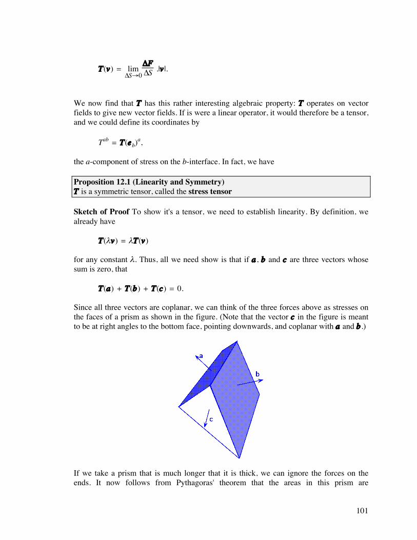
101

T(v) = lim ∆S→0

∆F∆S .|v|.

We now find that T has this rather interesting algebraic property: T operates on vector fields to give new vector fields. If is were a linear operator, it would therefore be a tensor, and we could define its coordinates by Tab = T(eb)

a, the a-component of stress on the b-interface. In fact, we have Proposition 12.1 (Linearity and Symmetry) T is a symmetric tensor, called the stress tensor Sketch of Proof To show it's a tensor, we need to establish linearity. By definition, we already have T(¬v) = ¬T(v) for any constant ¬. Thus, all we need show is that if a , b and c are three vectors whose sum is zero, that T(a) + T(b) + T(c) = 0. Since all three vectors are coplanar, we can think of the three forces above as stresses on the faces of a prism as shown in the figure. (Note that the vector c in the figure is meant to be at right angles to the bottom face, pointing downwards, and coplanar with a and b .)

If we take a prism that is much longer that it is thick, we can ignore the forces on the ends. It now follows from Pythagoras' theorem that the areas in this prism are

102

proportional to the three vectors. Therefore, multiplying through by a constant reduces the equation to one about actual forces on the faces of the prism, with T(a) + T(b) + T(c) the resultant force (since the lengths of the vectors a , b and c are equal to the respective areas). If this force was not zero, then there would be a resultant force F on the prism, and hence an acceleration of its material. The trouble is, if we cut all the areas in half by scaling all linear dimensions down by a factor å, then the areas scale down by a factor of å2, whereas the volume (and hence mass) scales down by a factor å3. In other words, T(å2a) + T(å2b) + T(å2c) = å2F is the resultant force on the scaled version of the prism, whereas its mass is proportional to å3. Thus its acceleration is proportional to 1/å (using Newton's law). This means that, as å becomes small (and hence the prism shrinks** ) the acceleration becomes infinite—hardly a likely proposition. The argument that the resulting tensor is symmetric follows by a similar argument applied to a square prism; asymmetry would result in a rotational force on the prism, and its angular acceleration would become infinite as we scale down if this were not zero. ❉ The Relativistic Stress-Energy Tensor Now we would like to generalize the stress tensor to 4-dimensional space. First we set the scenario for our discussion: We now work in a 4-manifold M whose metric has signature (1, 1, 1, -1). We have already call such a manifold a locally Minkowskian 4-manifold. (All this means is that we are using different units for time in our MCRFs.) Example 12.2 Let M be Minkowski space, where one unit of time is defined to be the time it takes light to travel one spatial unit. (For example, if units are measured in meters, then a unit of time would be approximately 0.000 000 003 3 seconds.) In these units, c = 1, so the metric does have this form. The use of MCRFs allows us to define new physical scalar fields as follows: If we are, say, in the interior of a star (which we think of as a continuous fluid) we can measure the pressure at a point by hitching a ride on a small solid object moving with the fluid. Since this should be a smooth function, we consider the pressure, so measured, to be a scalar field. Mathematically, we are defining the field by specifying its value on MCRFs. Now, we would like to measure a 4-space analogue of the force exerted across a plane, except this time, the only way we can divide 4-space is by using a hyperplane; the span ** Honey, I shrank the prism.

103

of three vectors in some frame of reference. Thus, we seek a 4-dimensional analogue of the quantity n∆S. By coincidence, we just happen to have such a gizmo lying around: the Levi-Civita tensor. Namely, if a, b, and c are any three vectors in 4-space, then we can define an analogue of n∆S to be œijklaibkcl, where œ is the Levi-Civita tensor. (See the exercises.) Next, we want to measure stress by generalizing the classical formula

stress = T(n) = lim∆S→0

∆F∆S

for such a surface element. Hopefully, the space-coordinates of the stress will continue to measure force. The first step is to get rid of all mention of unit vectors—they just dont arise in Minkowski space (recall that vectors can be time-like, space-like, or null...). We first rewrite the formula as T(n∆S) = ∆F , the total force across the area element ∆S. Now multiply both sides by a time coordinate increment: T(n∆S∆x4) ≈ ∆F∆x4 ≈ ∆p , where p is the 3-momentum.# This is fine for three of the dimensions. In other words, T(n∆V) = ∆p , or T(∆V) = ∆p where V is volume in Euclidean 4-space, ∆V = n∆V, and where we take the limit as ∆V’0. But now, generalizing to 4-space is forced on us: first replace momentum by the 4-momentum P , and then, noting that n∆S∆x4 is a 3-volume element in 4-space (because it is a product of three coordinate increments), replace it by the correct analogue for Minkowski space, (∆V)i = œijkl∆x

j∆yk∆zl, getting T(∆V) = ∆P .... (I) where ∆P is 4-momentum exerted on the positive side of the 3-volume ∆V by the opposite side. But, there is a catch: the quantity ∆V has to be really small (in terms of

# Classically, force is the time rate of change of momentum.

104

coordinates) for this formula to be accurate. Thus, we rewrite the above formula in differential form: T(h3∆V) = P(h), and so

T(∆V) = limh→0 P(h)

h3

This describes T as a function which converts the covariant vector ∆V into a contravariant field (P), and thus suggests a type (2, 0) tensor. To get an honest tensor, we must define T on arbitrary covariant vectors (not just those of the form ∆V). However, every covariant vector Y* defines a 3-volume as follows. Recall that a one-form at a point p is a linear real-valued function on the tangent space Tp at that point. If it is non-zero, then its kernel, which consists of all vectors which map to zero, is a three-dimensional subspace of Tp. This describes (locally) a (hyper-)surface. (In the special case that the one-form is the gradient of a scalar field ˙, that surface coincides with the level hypersurface of ˙ passing through p.) If we choose a basis {v, w, u} for this subspace of Tp, then we can recover the one-form at p (up to constant multiples) by forming œijklv

jwkul.† This gives us the following formal definition of the tensor T at a point: Definition 12.3 (The Stress Energy Tensor) For an arbitrary covariant vector Y at p, we choose a basis {v, w, u} for its kernel, scaled so that Yi = œijklv

jwkul, and define T(Y) as follows: Form the parallelepiped ∆V = {r1v + rrw + r3u | 0 ≤ ri ≤ 1} in the tangent space, and compute, for each h > 0, the total 4-momentum P(h) exerted on the positive side1 of this volume element h3∆V element by the negative side. Then define

T(Y) =limh→0 P(h)

h3

Note Of course, physical reality intervenes here: how do you measure momentum across volume elements in the tangent space? Well, you do all your measurements in a locally inertial frame. Proposition 9.6 then guarantees that you get the same physical measurements near the origin regardless of the inertial frame you use (we are, after all, letting h approach zero). To evaluate its coordinates on an orthonormal (Lorentz) frame, we define Tab = T(eb)

a, † Indeed, all you have to check is that the covariant vector œijklv

jwkul has u, w, and v in its kernel. But that is immediate from the anti-symmetric properties of the Levi-Civita tensor. 1 “positive” being given by the direction of Y

105

so that we can take u, w, and v to be the other three basis vectors. Of interest to us is a more usable form—in terms of quantities that can be measured. For this, we need to move into an MCRF, and look at an example. Note It can be shown, by an argument similar to the one we used at the beginning of this section, that T is a symmetric tensor. Definition 12.4 Classically, a fluid has no viscosity if its stress tensor is diagonal in an MCFR (viscosity is a force parallel to the interfaces). Thus, for a viscosity-free fluid, the top 3¿3 portion of matrix should be diagonal in all MCRFs (independent of spacial axes). This forces it to be a constant multiple of the identity (since every vector is an eigenvector implies that all the eigenvalues are equal…). This single eigenvector measures the force at right-angles to the interface, and is called the pressure, p. Question Why the pressure? Answer Let us calculate T11 (in an MCRF). It is given. using (I), by

T11 = T(e1)1 = ∆P1

∆V , where the 4-momentum is obtained physically by suddenly removing all material on the positive side of the x1-axis, and then measuring 1-component of the 4-momentum at the origin. Since we are in an MCRF, we can use the SR 4-velocity formula: P = m0(v1, v2, v3, 1)/ 1-v2/c2 . At the instant the material is removed, the velocity is zero in the MCRF, so P(t=0) = m0(0, 0, 0, 1). After an interval ∆t in this frame, the 4-momentum changes to P(t=1) = m0(∆v, 0, 0, 1)/ 1-(∆v)2/c2 , since there is no viscosity (we must take ∆v2 = ∆v3 = 0 or else we will get off-diagonal spatial terms in the stress tensor). Thus, ∆P = m0(∆v, 0, 0, 1)/ 1-(∆v)2/c2 . This gives

106

(∆P)1 = m0∆v

1-(∆v)2/c2 = m∆v (m is the apparent mass)

= ∆(mv) = Change of measured momentum Thus,

∆P1

∆V = ∆(mv)∆y∆z∆t =

∆F∆y∆z (force = rate of change of momentum)

and we interpret force per unit area as pressure. What about the fourth coordinate? The 4th coordinate of the 4-momentum is the energy. A component of the form T4,1 measures energy-flow per unit time, per unit area, in the direction of the x1-axis. In a perfect fluid, we insist that, in addition to zero viscosity, we also have zero heat conduction. This forces all these off-diagonal terms to be zero as well. Finally, T44 measures energy per unit volume in the direction of the time-axis. This is the total energy density, ®. Think of is as the “energy being transferred from the past to the future.” This gives the stress-energy tensor in a comoving frame of the particle as

T =

⎣⎢⎡

⎦⎥⎤p 0 0 0

0 p 0 00 0 p 00 0 0 ®

.

What about other frames? To do this, all we need do is express T as a tensor whose coordinates in a the comoving frame happen to be as above. To help us, we recall from above that the coordinates of the 4-velocity in the particle's frame are u = [0 0 0 1] (just set v = 0 in the 4-velocity). (It follows that

uaub =

⎣⎢⎡

⎦⎥⎤0 0 0 0

0 0 0 00 0 0 00 0 0 1

in this frame.) We can use that, together with the metric tensor

g =

⎣⎢⎡

⎦⎥⎤1 0 0 0

0 1 0 00 0 1 00 0 0 -1

107

to express T as Tab = (® + p)uaub + pgab. Stress-Energy Tensor for Perfect Fluid The stress-energy tensor of a perfect fluid (no viscosity and no heat conduction) is given at a point m é M by Tab = (® + p)uaub + pgab, where: ® is the mass energy density of the fluid p is the pressure ui is its 4-velocity Note that the scalars in this definition are their physical magnitudes as measured in a MCRF. Conservation Laws Let us now go back to the general formulation of T (not necessarily in a perfect fluid), work in an MCRF, and calculate some covariant derivatives of T. Consider a little cube with each side of length ∆l, oriented along the axes (in the MCRF). We saw above that T41 measures energy-flow per unit time, per unit area, in the direction of the x1-axis. Thus, the quantity T41

,1∆l is the approximate increase of that quantity (per unit area per unit time). Thus, the increase of outflowing energy per unit time in the little cube is T41

,1(∆l)3

due to energy flow in the x1-direction. Adding the corresponding quantities for the other directions gives

- ∂E∂t = T41

,1(∆l)3 + T42

,2(∆l)3 + T43

,3(∆l)3,

which is an expression of the law of conservation of energy. Since E is given by T44(∆l)3, and t = x4, we therefore get - T44

,4 (∆l)3 = (T41

,1 + T42,2 + T43

,3)(∆l)3,

108

giving T41

,1 + T42,2 + T43

,3 + T44,4 = 0

A similar argument using each of the three components of momentum instead of energy now gives us the law of conservation of momentum (3 coordinates): Ta1

,1 + Ta2,2 + Ta3

,3 + Ta4,4 = 0

for a = 1, 2, 3. Combining all of these and reverting to an arbitrary frame now gives us:

Einstein's Conservation Law Ô.T = 0 where Ô.T is the contravariant vector given by (Ô.T)j = Tjk

|k. This law combines both energy conservation and momentum conservation into a single elegant law. Exercise Set 12 1. If a, b, and c are any three vector fields in locally Minkowskain 4-manifold, show that the field œijklaibkcl is orthogonal to a, b, and c .(œ is the Levi-Civita tensor.) 2. Why can’t we just write any (covariant) vector like ∆V as ∆V = n∆V where n is a unit vector (||n||2 = ±1)?

109

13. Three Basic Premises of General Relativity Spacetime General relativity postulates that spacetime (the set of all events) is a smooth 4-dimensional Riemannian manifold M, where points are called events, with the properties A1-A3 listed below. A1. Locally, M is Minkowski spacetime (so that special relativity holds locally). This means that, if we diagonalize the scalar product on the tangent space at any point, we obtain the matrix

⎣⎢⎡

⎦⎥⎤1 0 0 0

0 1 0 00 0 1 00 0 0 -1

The metric is measurable by clocks and rods. Before stating the next axiom, we recall some definitions. Definitions 13.1 Let M satisfy axiom A1. If Vi is a contravariant vector at a point in M, define ||Vi||2 = “Vi, Vi‘ = ViVjgij. (Note that we are not defining ||Vi|| here.) We say the vector Vi is timelike if ||Vi||2< 0, lightlike if ||Vi||2= 0, and spacelike if ||Vi||2> 0, Examples 13.2 (a) If a particle moves with constant velocity v in some Lorentz frame, then at time t = x4 its position is x = a + vx4. Using the local coordinate x4 as a parameter, we obtain a path in M given by

xi(x4) = ⎩⎪⎨⎪⎧a

i + vix4 if i = 1, 2, 3

x4 if i = 4

so that the tangent vector (velocity) dxi/dx4 has coordinates (v1, v2, v3, 1) and hence square magnitude

110

||(v1, v2, v3, 1)||2 = |v|2 - c2. It is timelike at sub-light speeds, lightlike at light speed, and spacelike at faster-than-light speeds. (b) If u is the 4-velocity dxi/d† of some particle in locally Minkowskian spacetime, then we saw (normal condition in Section 11) that “u, u‘ = -c2 = -1 in our units. A2. Freely falling particles move on timelike geodesics of M. Here, a freely falling particle is one that is effected only by gravity, and recall that a timelike geodesic is a geodesic xi(t) with the property that ||dxi/dt||2 < 0 in any paramaterization. (This property is independent of the parameterization—see the exercise set.) A3 (Strong Equivalence Principle) All physical laws that hold in flat Minkowski space (ie. “special relativity”), are expressible in terms of vectors and tensors, and are meaningful in the manifold M, continue to hold in every frame (provided we replace derivatives by covariant derivatives). Note Here are some consequences: 1. No physical laws in GR can use the term “straight line,” since that concept has no meaning in M; what's straight in the eyes of one chart is curved in the eyes of another. “Geodesic,” on the other hand, does make sense, since it is independent of the choice of coordinates. 2. If we can write down physical laws, such as Maxwell's equations, that work in Minkowski space, then those same laws must work in curved space-time, without the addition of any new terms, such as the curvature tensor. In other words, there can be no form of Maxwell's equations for general curved spacetime that involve the curvature tensor. An example of such a law is the conservation law, Ô.T = 0, which is thus postulated to hold in all frames. A Consequence of the Axioms: Forces in Almost Flat Space Suppose now that the metric in our frame is almost Lorentz, with a slight, not necessarily constant, deviation ˙ from the Minkowski metric, as follows.

g** =

⎣⎢⎡

⎦⎥⎤1+2˙ 0 0 0

0 1+2˙ 0 00 0 1+2˙ 00 0 0 -1+2˙

…………

(I) or

111

ds2 = (1+2˙)(dx2 + dy2 + dz2) - (1-2˙)dt2. Notes 1. We are not in an inertial frame (modulo scaling) since ˙ need not be constant, but we are in a frame that is almost inertial. 2. The metric g** is obtained from the Minkowski g by adding a small multiple of the identity matrix. We shall see that such a metric does arise, to first order of approximation, as a consequence of Einstein's field equations. Now, we would like to examine the behavior of a particle falling freely under the influence of this metric. What do the timelike geodesics look like? Let us assume we have a particle falling freely, with 4-momentum P = m0U, where U is its 4-velocity, dxi/d†. The paramaterized path xi(†) must satisfy the geodesic equation, by A2. Definition 9.1 gives this as

d2xi

d†2 + ¶ris dxr

d† dxs

d† = 0.

Multiplying both sides by m0

2 gives

m0

d2(m0xi)

d†2 + ¶ris d(m0x

r)d†

d(m0xs)

d† = 0,

or

m0dPi

d† + ¶risP

rPs = 0 (since Pi = d(m0xi/d†))

where, by the (ordinary) chain rule (note that we are not taking covariant derivatives here... that is, dPi/d† is not a vector—see Section 8 on covariant differentiation),

dPi

d† = Pi,kdxk

d†

so that

Pi,kdm0x

k

d† + ¶risP

rPs = 0, or Pi

,kPk + ¶r

isP

rPs = 0 ………… (I)

112

Now let us do some estimation for slowly-moving particles v << 1 (the speed of light), where we work in a frame where g has the given form.‡ First, since the frame is almost inertial (Lorentz), we are close to being in SR, so that P* ‡ m0U* = m0[v1, v2, v3, 1] (we are taking c = 1here) ‡ [0, 0, 0, m0] (since v << 1) (in other words, the frame is almost comoving) Thus (I) reduces to Pi

,4m0 + ¶4i4 m0

2 = 0 ………… (II) Let us now look at the spatial coordinates, i = 1, 2, 3. By definition, ¶4

i4 =

12 gij(g4j,4 + gj4,4 - g44,j).

We now evaluate this at a specific coordinate i = 1, 2 or 3, where we use the definition of the metric g, recalling that g** = (g**)

-1, and obtain

12 (1+2˙)-1(0 + 0 - 2˙,i) ‡

12 (1-2˙)(-2˙,i) ‡ -˙,i.

(Here and in what follows, we are ignoring terms of order O(˙2).) Substituting this information in (II), and using the fact that

Pi,4 =

∂∂x4 (mov

i),

‡ Why don't we work in an inertial frame (the frame of the particle)? Well, in an inertial frame, we adjust the coordinates to make g = diag[1, 1, 1, -1] at the origin of our coordinate system. The first requirement of an inertail frame is that, ˙(0, 0, 0, 0) = 0. This you can certainly do, if you like; it doesn't effect the ensuing calculation at all. The next requirement is more serious: that the partial derivatives of the gij vanish. This would force the geodesics to be uninteresting (straight) at the origin, since the Christoffel symbols vanish, and (II) becomes Pi

|4P4 = 0,

that is, since P4 ‡ m0 and Pi|4 =

ddx4 (m0v

i) = rate of change of momentum, that

rate of change of momentum = 0, so that the particle is experiencing no force (even though it's in a gravitational field). Question But what does this mean? What is going on here? Answer All this is telling us is that an inertial frame in a gravitational field is one in which a particle experiences no force. That is, it is a “freely falling” frame. To experience one, try bungee jumping off the top of a tall building. As you fall, you experience no gravitational force—as though you were in outer space with no gravity present. This is not, however, the situation we are studying here. We want to be in a frame where the metric is not locally constant. so it would defeat the purpose to choose an inertial frame.

113

the time-rate of change of momentum, or the “force” as measured in that frame (see the exercise set), we can rewrite (II) as

m0∂∂x4 (mov

i) - m02˙,i = 0,

or

∂∂x4 (mov

i) - m0˙,i = 0.

Thinking of x4 as time t, and adopting vector notation for three-dimensional objects, we have, in old fashioned 3-vector notation,

∂∂t (mov) = m0Ô˙,

that is F = mÔ˙. This is the Newtonian force experienced by a particle in a force field potential of ˙. (See the exercise set.) In other words, we have found that we can duplicate, to a good approximation, the physical effects of Newton-like gravitational force from a simple distortion of the metric. In other words—and this is what Einstein realized—gravity is nothing more than the geometry of spacetime; it is not a mysterious “force” at all. Exercise Set 13 1. Show that, if xi = xi(t) has the property that ||dxi/dt||2 < 0 for some parameter t, then ||dxi/dts|2 < 0 for any other parameter s such that ds/dt ≠ 0 along the curve. In other words, the property of being timelike does not depend on the choice of paramaterization. 2. What is wrong with the following (slickly worded) argument based on the Strong Equivalence Principle?

I claim that there can be no physical law of the form A = R in curved spacetime, where A is some physical quantity and R is any quantity derived from the curvature tensor. (Since we shall see that Einstein's Field Equations have this form, it would follow from this argument that he was wrong!) Indeed, if the postulated law A = R was true, then in flat spacetime it would reduce to A = 0. But then we have a physical law A = 0 in SR, which must, by the Strong Equivalence Principle, generalize to A = 0 in curved spacetime as well. Hence the original law A = R was wrong.

3. Gravity and Antigravity Newton's law of gravity says that a particle of mass M exerts a force on another particle of mass m according to the formula

F = - GMmr

r3 ,

114

where r = “x, y, z‘, r = |r |, and G is a constant that depends on the units; if the masses M and m are given in kilograms, then G ‡ 6.67 ¿ 10-11, and the resulting force is measured in newtons.Î (Note that the magnitude of F is proportional to the inverse square of the distance r . The negative sign makes the force an attractive one.) Show by direct calculation that F = mÔ˙, where

˙ = GMr .

Hence write down a metric tensor that would result in an inverse square repelling force (“antigravity”). 14. The Einstein Field Equations and Derivation of Newton's Law Einstein's field equations show how the sources of gravitational fields alter the metric. They can actually be motivated by Newton's law for gravitational potential ˙, with which we begin this discussion. First, Newton's law postulates the existence of a certain scalar field ˙, called gravitational potential which exerts a force on a unit mass given by F = Ô˙ (classical gravitational field) Further, ˙ satisfies Ô2˙ = Ô.(Ô˙) = 4πG® ... (I) Div(gravitational field) = constant ¿ mass density where ® is the mass density and G is a constant. (The divergence theorem then gives the more familiar F = Ô˙ = GM/r2 for a spherical source of mass M—see the exercise set.) In relativity, we need an invariant analogue of (I). First, we generalize the mass density to energy density (recall that energy and mass are interchangeable according to relativity), which in turn is only one of the components of the stress-energy tensor T. Thus we had better use the whole of T. Question What about the mysterious gravitational potential ˙? Answer That is a more subtle issue. Since the second principle of general relativity tells us that particles move along geodesics, we should interpret the gravitational potential as somehow effecting the geodesics. But the most fundamental determinant of geodesics is the underlying metric g. Thus we will generalize ˙ to g. In other words, Einstein replaced Î A Newton is the force that will cause a 1-kilogram mass to accelerate at 1 m/sec2.

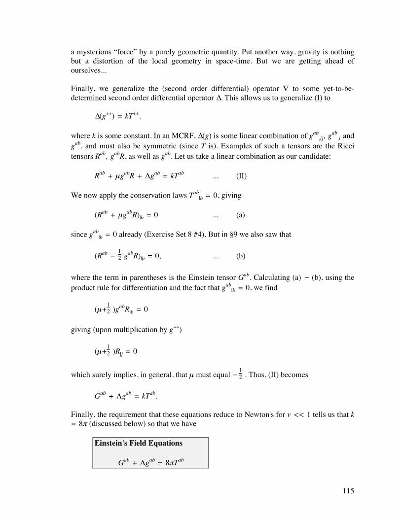
115

a mysterious “force” by a purely geometric quantity. Put another way, gravity is nothing but a distortion of the local geometry in space-time. But we are getting ahead of ourselves... Finally, we generalize the (second order differential) operator Ô to some yet-to-be-determined second order differential operator ∆. This allows us to generalize (I) to ∆(g**) = kT**, where k is some constant. In an MCRF, ∆(g) is some linear combination of gab

,ij, gab

,i and gab, and must also be symmetric (since T is). Examples of such a tensors are the Ricci tensors Rab, gabR, as well as gab. Let us take a linear combination as our candidate: Rab + µgabR + ¡gab = kTab ... (II) We now apply the conservation laws Tab

|b = 0, giving (Rab + µgabR)|b = 0 ... (a) since gab

|b = 0 already (Exercise Set 8 #4). But in §9 we also saw that (Rab -

12 g

abR)|b = 0, ... (b) where the term in parentheses is the Einstein tensor Gab. Calculating (a) - (b), using the product rule for differentiation and the fact that gab

|b = 0, we find (µ+

12 )g

abR|b = 0

giving (upon multiplication by g**)

(µ+12 )R|j = 0

which surely implies, in general, that µ must equal -

12 . Thus, (II) becomes

Gab + ¡gab = kTab. Finally, the requirement that these equations reduce to Newton's for v << 1 tells us that k = 8π (discussed below) so that we have

Einstein's Field Equations Gab + ¡gab = 8πTab

116

The constant ¡ is called the cosmological constant. Einstein at first put ¡ = 0, but later changed his mind when looking at the large scale behavior of the universe. Later still, he changed his mind again, and expressed regret that he had ever come up with it in the first place. The cosmological constant remains a problem child to this day.† We shall set it equal to zero. Solution of Einstein's Equations for Static Spherically Symmetric Stars In the case of spherical symmetry, we use polar coordinates (r, ø, ˙, t) with origin thought of as at the center of the star as our coordinate system (note it is singular there, so in fact this coordinate system does not include the origin) and restrict attention to g of the form

g** =

⎣⎢⎢⎡

⎦⎥⎥⎤grr 0 0 grt

0 r2 0 00 0 r2sin2ø 0grt 0 0 -gtt

,

or ds2 = 2grt dr dt + grr dr

2 + r2 dø2 + r2

sinø d˙2 - gt dt2,

where each of the coordinates is a function of r and t only. In other words, at any fixed time t, the surfaces ø = const, ˙ = const and r = const are all orthogonal. (This causes the zeros to be in the positions shown.) Question Explain why the non-zeros terms have the above form. Answer For motivation, let us first look at the standard metric on a 2-sphere of radius r: (see Example 5.2(d))

g** = ⎣⎢⎡

⎦⎥⎤r2 0

0 r2sin2ø .

† The requirement that Newton's laws be the limit of general relativity for small v forces lambda to be very small. Setting it equal to zero gives all the correct predictions for the motions of planets to within measurable accuracy. Put another way, if ¡ ≠ 0, then experimental data shows that it must be very small indeed. Also, we could take that term over to the right-hand side of the equation and incorporate it into the stress-energy tensor, thus regarding -¡gab/8π as the stress-energy tensor of empty space. Following is an excerpt from an article in Scientific American (September, 1996, p. 22):

… Yet the cosmological constant itself is a source of much puzzlement. Indeed, Christopher T. Hill of Fermilab calls it “the biggest problem in all of physics.” Current big bang models require that lambda is small or zero, and various observations support that assumption. Hill points out, however, that current particle physics theory predicts a cosmological constant much, much greater—by a factor of at least 1052, large enough to have crunched the universe back down to nothing immediately after the big bang. “Something is happening to suppress this vacuum density,” says Alan Guth of MIT, one of the developers of the inflationary theory. Nobody knows, however, what that something is …

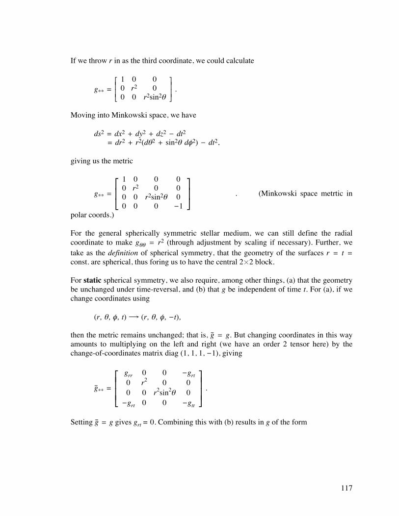
117

If we throw r in as the third coordinate, we could calculate

g** = ⎣⎢⎢⎡

⎦⎥⎥⎤1 0 0

0 r2 00 0 r2sin2ø

.

Moving into Minkowski space, we have ds2 = dx2 + dy2 + dz2 - dt2 = dr2 + r2(dø2 + sin2ø d˙2) - dt2, giving us the metric

g** =

⎣⎢⎡

⎦⎥⎤1 0 0 0

0 r2 0 00 0 r2sin2ø 00 0 0 -1

. (Minkowski space metrtic in

polar coords.) For the general spherically symmetric stellar medium, we can still define the radial coordinate to make gøø = r2 (through adjustment by scaling if necessary). Further, we take as the definition of spherical symmetry, that the geometry of the surfaces r = t = const. are spherical, thus foring us to have the central 2¿2 block. For static spherical symmetry, we also require, among other things, (a) that the geometry be unchanged under time-reversal, and (b) that g be independent of time t. For (a), if we change coordinates using (r, ø, ˙, t) ’ (r, ø, ˙, -t), then the metric remains unchanged; that is, g– = g. But changing coordinates in this way amounts to multiplying on the left and right (we have an order 2 tensor here) by the change-of-coordinates matrix diag (1, 1, 1, -1), giving

g–** =

⎣⎢⎢⎡

⎦⎥⎥⎤grr 0 0 -grt

0 r2 0 00 0 r2sin2ø 0

-grt 0 0 -gtt

.

Setting g– = g gives grt = 0. Combining this with (b) results in g of the form

118

g** =

⎣⎢⎢⎡

⎦⎥⎥⎤e2¡ 0 0 0

0 r2 0 00 0 r2sin2ø 00 0 0 -e2∞

,

where we have introduced the exponentials to fix the signs, and where ¡ = ¡(r), and ∞ = ∞(r). Using this version of g, we can calculate the Einstein tensor to be (see the exercise set!) G** =

⎣⎢⎢⎡

⎦⎥⎥⎤

2r∞'e-4¡-

1r2e-2¡(1-e-2¡) 0 0 0

0e-2¡

r2 [∞''+(∞')2+∞'r -∞'¡'-

¡'r ] 0 0

0 0Gøø

sin2ø0

0 0 01r2 e

-2∞ ddr[r(1-e-2¡)]

We also need to calculate the stress energy tensor, Tab = (®+p)uaub + pgab. In the static case, there is assumed to be no flow of star material in our frame, so that u1 = u2 = u3 = 0. Further, the normal condition for four velocity, “u, u‘ = -1, gives

[0, 0, 0, u4]

⎣⎢⎢⎡

⎦⎥⎥⎤e2¡ 0 0 0

0 r2 0 00 0 r2sin2ø 00 0 0 -e2∞

⎣⎢⎡

⎦⎥⎤0

00u4

= -1

whence u4 = e-∞, so that T44 = (®+p)e-2∞ + p(-e-2∞) (note that we are using g** here). Hence, T** = (® + p)u*u* + pg**

=

⎣⎢⎡

⎦⎥⎤0 0 0 0

0 0 0 00 0 0 00 0 0 (®+p)e-2∞

+ p

⎣⎢⎢⎡

⎦⎥⎥⎤e-2¡ 0 0 0

01r2 0 0

0 01

r2sin2ø0

0 0 0 -e-2∞

119

=

⎣⎢⎢⎡

⎦⎥⎥⎤pe-2¡ 0 0 0

0pr2 0 0

0 0p

r2sin2ø0

0 0 0 ®e-2∞

.

(a) Equations of Motion Tab

|b = 0 To solve these, we first notice that we are not in an inertial frame (the metric g is not nice at the origin; in fact, nothing is even defined there!) so we need the Christoffel symbols, and use

Tab|b =

∂Tab

∂xb + ¶kabT

kb + ¶bbkT

ak,

where

¶hpk =

12 glp

⎝⎜⎛

⎠⎟⎞∂gkl

∂xh + ∂glh

∂xk - ∂ghk

∂xl .

Now, lots of the terms in Tab

|b vanish by symmetry, and the restricted nature of the functions. We shall focus on a = 1, the r-coordinate. We have: T1b

|b = T11|1 + T12

|2 + T13|3 + T14

|4 , and we calculate these terms one-at-a-time.

a = 1, b = 1: T11|1 =

∂T11

∂x1 + ¶111T

11 + ¶111T

11.

To evaluate this, first look at the term ¶1

11:

¶111 =

12 g

l1(g1l,1 + gl1,1 - g11,l)

= 12 g

11(g11,1 + g11,1 - g11,1) (because g is diagonal, whence l = 1)

= 12 g

11(g11,1)

= 12 e

-2¡e2¡.2¡'(r) = ¡'(r). Hence,

T11|1 =

dpdr e

-2¡ + (- 2p¡'(r)e-2¡) + 2¡'(r)pe-2¡ = dpdr e

-2¡. Now for the next term:

120

a = 1, b = 2: T12|2 =

∂T12

∂x2 + ¶212T

22 + ¶221T

11

= 0 + 12 g

l1(g2l,2+gl2,2-g22,l)T22 +

12 g

l2(g1l,2+gl2,1-g21,l)T11

= 12 g

11(-g22,1) T22+

12 g

22(g22,1)T11

= 12 e

-2¡(-2r)pr2 +

12

1r2 2rpe

-2¡

= 0. Similarly (exercise set) T13

|3 = 0. Finally,

a = 1, b = 4: T14|4 =

∂T14

∂x4 + ¶414T

44 + ¶441T

11

= 12 g

11(-g44,1) T44+

12 g

44(g44,1)T11

= 12 e

-2¡(2∞'(r)e2∞)®e-2∞ + 12 (-e-2∞)(-2∞'(r)e2∞)pe-2¡

= e-2¡∞'(r)[® + p]. Hence, the conservation equation becomes T1a

|a = 0

⇔ ⎝⎜⎛

⎠⎟⎞dp

dr + d∞dr (®+p) e-2¡ = 0

⇔ dpdr = -(®+p)

d∞dr .

This gives the pressure gradient required to keep the plasma static in a star. Note In classical mechanics, the term on the right has ® rather than ®+p. Thus, the pressure gradient is larger in relativistic theory than in classical theory. This increased pressure gradient corresponds to greater values for p, and hence bigger values for all the components of T. By Einstein's field equations, this now leads to even greater values of ∞ (manifested as gravitational force) thereby causing even larger values of the pressure gradient. If p is large to begin with (big stars) this vicious cycle diverges, ending in the gravitational collapse of a star, leading to neutron stars or, in extreme cases, black holes.

121

(b) Einstein Field Equations Gab = 8πTab Looking at the (4,4) component first, and substituting from the expressions for G and T, we find

1r2 e

-2∞ ddr [ ]r(1-e-2¡) = 8π®e-2∞.

If we define

12 r(1-e-2¡) = m(r),

then the equation becomes

1r2 e

-2∞dm(r)dr = 4π®e-2∞,

or

dm(r)dr = 4πr2® …… (I)

This looks like an equation for classical mass, since classically,

M(R) = ∫∫R0 4πr2®(r) dr where the integrand is the mass of a shell whose thickness is dr. Thus,

dM(R)dr = 4π2®(r).

Here, ® is energy density, and by our choice of units, energy is equal to rest mass, so we interpret m(r) as the total mass of the star enclosed by a sphere of radius r. Now look at the (1, 1) component:

2r ∞'e-4¡ -

e-2¡

r2 (1-e-2¡) = 8πpe-2¡

⇒ 2r ∞' -

e2¡

r2 (1-e-2¡) = 8πpe2¡

⇒ ∞' = e2¡ (1-e-2¡) + 8πr2p2r .

122

In the expression for m, solve for e2¡ to get

e2¡ = 1

1-2m/r ,

giving

d∞dr =

8πr2p + 2m/r2r(1-2m/r) ,

or

d∞dr =

4πr3p + m r(r-2m) ……… (II)

It can be checked using the Bianchi identities that we in fact get no additional information from the (2,2) and (3,3) components, so we ignore them. Consequences of the Field Equations: Outside the Star Outside the star we take p = ® ‡ 0, and m(r) = M, the total stellar mass, getting

(I): dmdr = 0 (nothing new, since m = M = constant)

(II): d∞dr = M

r(r-2M) , which is a separable first order differential equation with solution

e2∞ = 1 - 2Mr .

if we impose the boundary condition ∞’0 as r’+Ï. (See the exercise Set). Recalling from the definition of m that

e2¡ = 1

1-2M/r , we can now express the metric outside a star as follows:

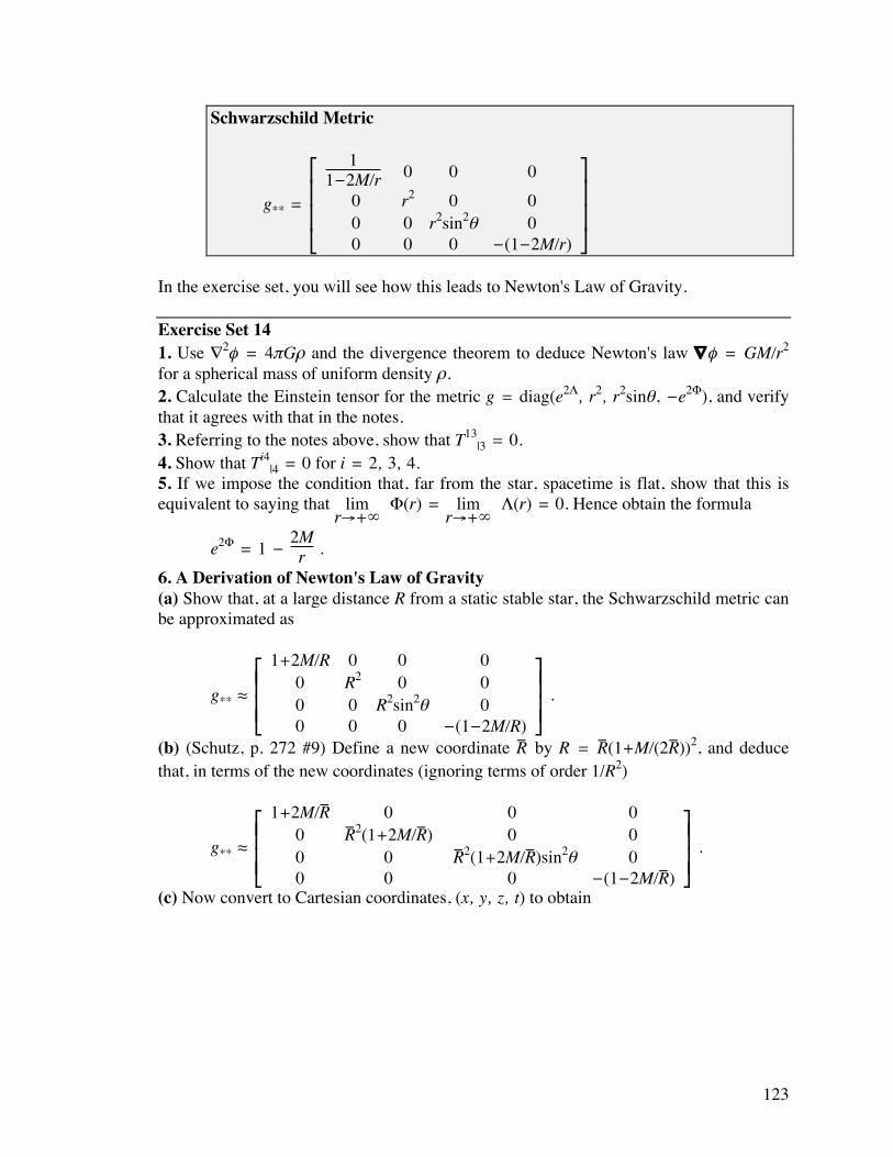
123

Schwarzschild Metric

g** =

⎣⎢⎢⎡

⎦⎥⎥⎤1

1-2M/r 0 0 0

0 r2 0 00 0 r2sin2ø 00 0 0 -(1-2M/r)

In the exercise set, you will see how this leads to Newton's Law of Gravity. Exercise Set 14 1. Use Ô2˙ = 4πG® and the divergence theorem to deduce Newton's law Ô˙ = GM/r2 for a spherical mass of uniform density ®. 2. Calculate the Einstein tensor for the metric g = diag(e2¡, r2, r2sinø, -e2∞), and verify that it agrees with that in the notes. 3. Referring to the notes above, show that T13

|3 = 0. 4. Show that Ti4

|4 = 0 for i = 2, 3, 4. 5. If we impose the condition that, far from the star, spacetime is flat, show that this is equivalent to saying that lim

r→+Ï ∞(r) = lim

r→+Ï ¡(r) = 0. Hence obtain the formula

e2∞ = 1 - 2Mr .

6. A Derivation of Newton's Law of Gravity (a) Show that, at a large distance R from a static stable star, the Schwarzschild metric can be approximated as

g** ‡

⎣⎢⎢⎡

⎦⎥⎥⎤

1+2M/R 0 0 00 R2 0 00 0 R2sin2ø 00 0 0 -(1-2M/R)

.

(b) (Schutz, p. 272 #9) Define a new coordinate R— by R = R—(1+M/(2R—))2, and deduce that, in terms of the new coordinates (ignoring terms of order 1/R2)

g** ‡

⎣⎢⎢⎡

⎦⎥⎥⎤

1+2M/R— 0 0 00 R—2(1+2M/R—) 0 00 0 R—2(1+2M/R—)sin2ø 00 0 0 -(1-2M/R—)

.

(c) Now convert to Cartesian coordinates, (x, y, z, t) to obtain

124

g** ‡

⎣⎢⎡

⎦⎥⎤1+2M/R— 0 0 0

0 1+2M/R— 0 00 0 1+2M/R 00 0 0 -(1-2M/R—)

.

(d) Now refer to the last formula in Section 13, and obtain Newton's Law of Gravity. To how many kilograms does one unit of M correspond? 15. The Schwarzschild Metric and Event Horizons We saw that the metric outside a spherically symmetric static stable star (Schwarzschild metric) is given by

ds2 = 1

1-2M/r dr2 + r2d¢2 - (1-2M/r)dt2,

where d¢2 = dø2 + sin2ø d˙2. We see immediately that something strange happens when 2M = r, and we look at two cases. Case 1 (Not-So-Dense Stars) Radius of the star, rs > 2M. If we recall that the Schwarzschild metric is only valid for outside a star; that is, r > rs, we find that r > 2M as well, and so 1-2M/r is positive, and never zero. (If r ≤ 2M, we are inside the star, and the Schwarzschild metric no longer applies.)

r = 2M

rs

r

Case 2 (Extremely Dense Stars) Radius of the star, rs < 2M. Here, two things happen: First, as a consequence of the equations of motion, it can be shown that in fact the pressure inside the star is unable to hold up against the gravitational forces, and the star collapses (see the next section) overwhelming even the quantum mechanical forces. In fact, it collapses to a singularity, a point with infinite density and no physical dimension, a black hole. For such objects, we have two distinct regions, defined by r > 2M and r < 2M, separated by the event horizon, r = 2M, where the metric goes infinite.

125

(r = 2M)

rs

Event Horizon(r = 2M)

Event Horizon

Gravitational Collapse

Particles Falling Inwards Suppose a particle is falling radially inwards. Let us see how long, on the particle's clock (proper time), it takes to reach the event horizon. Out approach will be as follows: (1) Use the principle that the path is a geodesic in space time. (2) Deduce information about dr/d†. (3) Integrate d† to see how long it takes. Recall first the geodesic equation for such a particle, Pi

|kPk + ¶r

isP

rPs = 0. We saw in the derivation (look back) that it came from the equation

m0dPi

d† + ¶risP

rPs = 0 ……… (I) There is a covariant version of this:

m0dPsd† - ¶r

isP

rPi = 0.

Derivation This is obtained as follows: Multiplying both sides of (I) by gia gives

m0dPi

d† gia + ¶risP

rPsgia = 0, or

m0d(giaP

i)d† - m0

dgiad† Pi+ ¶r

isP

rPsgia = 0

m0d(Pa)d† - m0

dgiad† Pi+ ¶r

isP

rPsgia = 0

126

m0d(Pa)d† - m0P

i(DgiaD† + ¶r

ki gka

dxr

d† + ¶akr gik

dxr

d† ) + ¶risP

rPsgia = 0

|| (by definition of Dgia/D†) 0

m0d(Pa)d† - ¶r

kiP

iPrgka - ¶akrP

iPrgik + ¶risP

rPsgia = 0, leaving

m0d(Pa)d† - ¶a

krP

iPrgik = 0, or

m0d(Pa)d† - ¶a

krPkP

r = 0, which is the claimed covariant version.

Now take this covariant version and write out the Christoffel symbols:

m0dPsd† = ¶r

isP

rPi

m0dPsd† =

12 gik(grk,s + gks,r - gsr,k) P

rPi

m0dPsd† =

12 (grk,s + gks,r - gsr,k) P

rPk But the sum of the second and third terms in parentheses is skew-symmetric in r and k, whereas the term outside is symmetric in them. This results in them canceling when we sum over repeated indices. Thus, we are left with

m0dPsd† =

12 grk,sP

rPk ……… (II) But by spherical symmetry, g is independent of xi if i = 2, 3, 4. Therefore grk,s = 0 unless s = 1. This means that P2, P3 and P4 are constant along the trajectory. Since P4 is constant, we define E = -P4/m0, another constant. Question What is the meaning of E? Answer Recall that the fourth coordinate of four momentum is the energy. Suppose the particle starts at rest at r = Ï and then falls inward. Since space is flat there, and the particle is at rest, we have

127

P* = [0, 0, 0, m0] (fourth coordinate is rest energy = m0) (which corresponds to P* = [0, 0, 0, -m0], since P* = P*g**). Thus, E = -P4/m0 = 1, the rest energy per unit mass. As the particle moves radially inwards, P2 = P3 = 0. What about P1? Now we know the first coordinate of the contravariant momentum is given by

P1 = m0drd† (by definition, Pi = m0

dxi

d† , and x1 = r)

Thus, using the metric to get the fourth contravariant coordinate,

P* = (m0drd† , 0, 0, m0E(1-2M/r)-1)

we now invoke the normalization condition {u, u‘ = -1, whence “P, P‘ = -m0

2, so that

-m02 = m0

2

⎝⎜⎛

⎠⎟⎞dr

d†

2

(1-2M/r)-1 - m02E2(1-2M/r)-1,

giving

⎝⎜⎛

⎠⎟⎞dr

d†

2

= E2 - 1 + 2M/r, which is the next step in our quest:

d† = - dr

E2-1+2M/r ,

where we have introduced the negative sign since r is a decreasing function of †. Therefore, the total time elapsed is

T = ⌡⎮⌠

R

2M

- dr

E2-1+2M/r ,

which, though improper, is finite.* This is the time it takes, on the hapless victim's clock, to reach the event horizon. * See Schutz, p. 289.

128

Now let's recalculate this from the point of view of an observer who is stationary with respect to the star. That is, let us use the coordinate x4 as time t. How is it related to proper time? Well, the four velocity tells how:

V4 = defn dx4

d† = dtd† .

We can get V4 from the formula for P* (and divide by m0) so that dt = V4d† = E(1-2M/r)-1 d† giving a total time of

T = ⌡⎮⌠

R

2M

- dr

E(1-2M/r) E2-1+2M/r .

This integral diverges! So, in the eyes of an outside observer, it takes that particle infinitely long to get there! Inside the Event Horizon—A Dialogue Tortoise: I seem to recall that the metric for a stationary observer (situated inside the event horizon) is still given by the Schwarzschild metric ds2 = (1-2M/r)-1dr2 + r2 d¢2 - (1-2M/r)dt2. Achilles: Indeed, but notice that now the coefficient of dr2 is negative, while that of dt2 is positive. What could that signify (if anything)? Tortoise: Let us do a little thought experiment. If we are unfortunate(?) enough to be there watching a particle follow either a null or timelike world line, then, with respect to any parameter (such as †) we must have dr/d† ≠ 0. In other words, r must always change with the parameter! Achilles: So you mean nothing can sit still. Why so? Tortoise: Simple. First: for any world line, the vector dxi/d† is non-zero, (or else it would not be a path at all!) so some coordinate must be non-zero. But now if we calculate ||dxi/d†||2 using the signature (-, +, +, +) we get

- something¿⎝⎜⎛

⎠⎟⎞dr

d†

2

+ something¿ the others,

129

so the only way the answer can come out zero or negative is if the first coordinate (dr/d†) is non-zero. Achilles: I think I see your reasoning... we could get a null path if all the coordinates were zero, but that just can't happen in a path! So you mean to tell me that this is true even of light beams. Mmm.... So you're telling me that r must change along the world line of any particle or photon! But that begs a question, since r is always changing with †, does it increase or decrease with proper time †? Tortoise: To tell you the truth, I looked in the Green Book, and all it said was the “obviously” r must decrease with †, but I couldn't see anything obvious about that. Achilles: Well, let me try a thought experiment for a change. If you accept for the moment the claim that a particle fired toward the black hole will move so as to decrease r, then there is at least one direction for which dr/d† < 0. Now imagine a particle being fired in any direction. Since dr/d† will be a continuous function of the angle in which the particle is fired, we conclude that it must always be negative. Tortoise: Nice try, my friend, but you are being too hasty (as usual). That argument can work against you: suppose that a particle fired away from the black hole will move (initially at least) so as to increase r, then your argument proves that r increases no matter what direction the particle is fired. Back to the drawing board. Achilles: I see your point... Tortoise (interrupting): Not only that. You might recall from Lecture 38 (or thereabouts) that the 4-velocity of as radially moving particle in free-fall is given by

V* = (drd† , 0, 0, E(1-2M/r)-1),

so that the fourth coordinate, dt/d† = E(1-2M/r)-1, is negative inside the horizon. Therefore, proper time moves in the opposite direction to coordinate time! Achilles: Now I'm really confused. Does this mean that for r to decrease with coordinate time, it has to increase with proper time? Tortoise: Yes. So you were (as usual) totally wrong in your reason for asserting that dr/d† is negative for an inward falling particle. Achilles: OK. So now the burden of proof is on you! You have to explain what the hell is going on. Tortoise: That's easy. You might dimly recall the equation

130

⎝⎜⎛

⎠⎟⎞dr

d†

2

= E2 - 1 + 2M/r on p. 112 of those excellent differential geometry notes, wherein we saw that we can take E = 1 for a particle starting at rest far from the black hole. In other words,

⎝⎜⎛

⎠⎟⎞dr

d†

2

= 2M/r. Notice that this is constant and never zero, so that dr/d† can never change sign during the trajectory of the particle, even as (in its comoving frame) it passes through the event horizon. Therefore, since r was initially decreasing with † (outside, in “normal” space-time), it must continue to do so throughout its world line. In other words, photons that originate outside the horizon can never escape in their comoving frame. Now (and here's the catch), since there are some particles whose world-lines have the property that the arc-length parameter (proper time) decreases with increasing r, and since r is the unique coordinate in the stationary frame that plays the formal role of time, and further since, in any frame, all world lines must move in the same direction with respect to the local time coordinate (meaning r) as their parameter increases, it follows that all world lines must decrease r with increasing proper time. Ergo, Achilles, r must always decrease with increasing proper time †. Of course, a consequence of all of this is that no light, communication, or any physical object, can escape from within the event horizon. They are all doomed to fall into the singularity. Achilles: But what about the stationary observer? Tortoise: Interesting point...the quantity dt/d† = E(1-2M/r)-1 is negative, meaning proper time goes in the opposite direction to coordinate time and also becomes large as it approaches the horizon, so it would seem to the stationary observer inside the event horizon that things do move out toward the horizon, but take infinitely long to get there. There is a catch, however, there can be no “stationary observer” according to the above analysis... Achilles: Oh. Exercise Set 15 1. Verify that the integral for the infalling particle diverges the case E = 1. 2. Mini-Black Holes How heavy is a black hole with event horizon of radius one meter? [Hint: Recall that the “M” corresponds to G¿total mass.] 3. Calculate the Riemann coordinates of curvature tensor Rabcd at the event horizon. r = 2M.

131

16. White Dwarfs, Neutron Stars and Black Holes—Guest Lecture by Gregory C. Levine I Introduction In this section we will look at the physical mechanisms responsible for the formation compact stellar objects. Compact objects such as white dwarf stars, neutron stars, and ultimately black holes, represent the final state of a star's evolution. Stars are born in gaseous nebulae in which clouds of hydrogen coalesce becoming highly compressed and heated through the gravitational interaction. At a temperature of about 107 K, a nuclear reaction begins converting hydrogen into the next heavier element, helium, and releasing a large quantity of electromagnetic energy (light). The helium accumulates at the center of the star and eventually becomes compressed and heated enough (108 K) to initiate nuclear fusion of helium into heavier elements. So far, the star is held in "near-equilibrium" by the countervailing forces of gravity, which compresses the star, and pressure from the vast electromagnetic energy produced during nuclear fusion, which tends to make it expand. However, as the star burns hotter and ignites heavier elements which accumulate in the core, electromagnetic pressure becomes less and less effective against gravitational collapse. In most stars, this becomes a serious problem when the core has reached the carbon rich phase but the temperature is still insufficient to fuse carbon into iron. Even if a star has reached sufficient temperature to create iron, no other nuclear fusion reactions producing heavier elements are exothermic and the star has exhausted its nuclear fuel. Without electromagnetic energy to hold the core up, one would think that the core would become unstable and begin to collapse---but another mechanism intervenes. II The Electron Gas But there is another "force" that holds the core up; now we will turn to a study of this force and how the balance between this force and gravity lead to the various stellar compact objects: white dwarfs, neutron stars and black holes. The stabilizing force that keeps the stellar core from collapsing operates at terrestrial scales as well. All solid matter resists compression and we will trace the origin of this behavior in a material that turns out to most resemble a stellar compact object: ordinary metal. Although metal is "hard" by human standards, it is to some degree elastic---capable of stretching and compression. Metals all have a similar atomic structure. Positively charged metal ion cores form a regular crystalline lattice and negatively charged valence electrons form a kind of gas that uniformly permeates the lattice.

132

+ ++ + +

++ + +

+ ++ + +

+ ++ + +

+

Suprisingly, the bulk properties of the metal such as heat capacity, compressibility, and thermal conductivity are almost exclusively properties of the electron gas and not the underlying framework of the metal ion cores. We will begin by studying the properties of an electron gas alone and then see if it is possible to justify such a simple model for a metal (or a star). To proceed, two very important principles from Quantum Mechanics need to be introduced: Pauli Exclusion Principle: Electrons cannot be in the same quantum state. For our purposes, this will effectively mean that electrons cannot be at the same point in space. Heisenberg Uncertainty Principle: A quantum particle has no precise position, x, or momentum, p. However, the uncertainties in the outcome of experiment aimed at simultaneously determining both quantities is constrained in the following way. Upon repeated measurements, the "spread" in momentum, ∆p, of a particle absolutely confined to a region in space of size∆x, is constrained by

∆x∆p ≥ 2

where ‡ 6.6¿10-34 Joule-sec is a fundamental constant of nature (the Planck constant). Here is how these two laws act together to give one of the familiar properties of metals. The Pauli Exclusion Principle tends to make electrons stay as far apart as possible. Each of N electrons confined in a box of volume R3 will typically have R3/N space of its own. Therefore, the average interparticle spacing is a0 = R/N1/3. (The situation is actually a bit more complicated than this *link*). Since the electrons are spatially confined within a region of linear size a0, the uncertainty in momentum is ∆p ‡ /a0. The precise meaning of ∆p2 is the variance of a large set of measurements of momentum. Denoting average by angle brackets, ∆p2 = “(p - “p‘)2‘ = “p2‘ - “p‘2. Therefore, the average value of p2 must be greater than or equal to∆p2.

133

Based on these results, let us calculate how the energy of an electron gas depends upon the size of the box containing it. The kinetic energy of a particle of mass m and speed v is

œ = 12 mv2 =

p2

2m

Now, taking the minimum value of momentum, p2 ‡ ∆p2 ‡ 2/a0

2, we arrive at the energy, œ = 2/mea0

2,, for a single electron of mass me. The total kinetic energy of N electrons is then Ee = Nœ. Finally, putting in the dependence of a0 on N and the system size, R, we get for Ee,

Ee ‡ 2

meR2 N5/3.

As the system size R is reduced, the energy increases. Even though the electrons do not interact with one another, there is an effective repulsive force resisting compression. The origin of this force is the uncertainty principle! (neglecting e-e interactions and neglecting temperature.) Let us test out this model by calculating the compressibility of metal. Consider a metal block that undergoes a small change in volume, ∆V, due to an applied pressure P.

P

6V

The bulk modulus, B, is defined as the constant of proportionality between the applied pressure and the fractional volume change.

P = B∆VV .

The outward pressure (towards positive R) exerted by the electron gas is defined in the usual way in terms of a derivative of the total energy of the system:

134

P = FA = -

1A ∂Ee

∂R The bulk modulus is then defined as

B = V∂P∂V = -

59 2me

⎝⎜⎛⎠⎟⎞N

V 5/3

‡ 10-10 - 10-11 N/m2.

(We've taken the volume per electron to be 1 nm3.) The values of B for Steel and Aluminum are Bsteel ‡ 6¿10-10 N/m2 and BAl ‡ 2¿10-10 N/m2. It is hard to imagine that this excellent agreement in magnitude is wholly fortuitous (it is not). Having seen that the Heisenberg uncertainty principle is the underlying physics behind the rigidity of metal, we will now see that it is also physical mechanism that keeps stars from collapsing under their own weight. III Compact Objects A star can only be in a condition of static equilibrium if there is some force to counteract the compressive force of gravity. In large stars this countervailing force is the radiation pressure from thermally excited atoms emitting light. But in a white dwarf star, the force counteracting gravity has its origin in the uncertainty principle, as it did in a metal. The elements making up the star (mostly iron) exist in a completely ionized state because of the high temperatures. One can think of the star as a gas of positive charge atomic nuclei and negative charge electrons. Each metal nucleus is a few thousand times heavier than the set of electrons that were attached to it, so the nuclei (and not the electrons) are responsible for the sizable gravitational force holding the star together. The electrons are strongly electrostatically bound to core of the star and therefore coexist in the same volume as the nuclear core---gravity pulling the nuclei together and the uncertainty principle effectively pushing the electrons apart.

+

++ ++

++ ++

++ +

We will proceed in the same way as in the calculation of the bulk modulus by finding an expression for the total energy and taking its derivative with respect to R to find the effective force. The gravitational potential energy of sphere of mass M and radius R is approximately

135

Eg ‡ - GM2

R where G ‡ 7 ¿ 10-11 Nm2/kg2 is the gravitational constant. (The exact result has a coeffient of order unity in front; we are doing only "order-of-magnitude" calculations and ignoring such factors.) The negative sign means that the force of gravity is attractive---energy decreases with decreasing R. We would like to express Eg in terms of N, like Ee---this will make the resulting expressions easier to adapt to neutron stars later on. The mass M of the star is the collective mass of the nucleons, to an excellent approximation. As you may know from chemisty, the number of nucleons (protons and neutrons) is roughly double the number of electrons, for light elements. If µ is the average number of nucleons per electron, for the heavier elements making up the star, The mass of the star is expressed as M=µmnN. Putting the expressions for the electron kinetic energy and the gravitational potential energy together, we get the total energy E:

E = Ee + Eg ‡ 2N5/3

meR2 - Gµ2mn

2N2

R .

The graph of the function E(R)

E

RR

reveals that there is a radius at which the energy is minimum---that is to say, a radius R0 where the force F = -∂E/∂R is zero and the star is in mechanical equilibrium. A rough calculation of R0 gives:

R0 = 2N-1/3

Gmeµ2mn2 ‡ 107 m = 10,000 km.

136

where we have used N ‡ 1057, a reasonable value for a star such as our sun. R0 corresponds to a star that is a little bigger than earth---a reasonable estimate for a white dwarf star! The mass density ® may also be calculated assuming the radius R0: ® ‡ 109 kg/m3 = 105 ¿ density of steel. On the average, the electrons are much closer to the nuclei in the white dwarf than they are in ordinary matter. Under some circumstances, the star can collapse to an object even more compact than a white dwarf---a neutron star. The Special Theory of Relatvity plays an important role in this further collapse. If we calculate the kinetic energy of the most energetic electrons in the white dwarf, we get:

œ ‡ 2

mea02 =

2me

⎝⎜⎛

⎠⎟⎞N

R0 2/3

‡ 100-14 Joules.

This energy is actually quite close to the rest mass energy of the electron itself, mec2 = 10-13 Joules. Recall that the expression for the kinetic energy, œ = p2/2m, is only a nonrelativistic approximation. Rest mass energy is a scalar formed from the product

pµpµ= œ2

c2 - p2 = (mc)2.

The exact expression for the energy œ of a relativistic particle is then:

œ = (pc)2+(mc2)2 = mc2 + p2

2m + terms of order ≥ ⎝⎜⎛

⎠⎟⎞p

mc4 .

When p ‡ mc (or, equivalently, when p2/m ‡ mc2 as above) the higher order terms cannot be neglected. Since the full expression for œ is unwieldy for our simple approximation schemes, we will look at the extreme relativistic limit, p >> mc. In this case, œ ‡ pc. This limit is effectively the limit for extremely massive stars, where the huge compressive force of gravity will force the electrons to have compensatingly high kinetic energies and enter the extreme relativistic regime. The different form for the energy of the electrons (now linear rather than quadratic in p) will have dramatic consequences for the stability equation for the radius R0 derived earlier. The calculation proceeds as before; according to the uncertainty principle the estimate for the momentum of an electron within the star is

p = a0

= N1/3

R .

Therefore, the total electron energy is given by

137

Ee ‡ Nœ ‡ Npc ‡ cN4/3

R The same expression as before for Eg results in the following expression for the total energy:

E + Ee + Eg ‡ cN4/3

R - Gµ2mn

2N2

R . The energy E(R) has a completely different behavior than in the nonrelativistic case. If we look at the force F = -∂E/∂R it is just equal to E/R. If the total energy is positive, the force always induces expansion; if the total energy is negative, the force always induces compression. Thus, if the total energy E is negative, the star will continue to collapse (with an ever increasing inward force) unless some other force intervenes. These behaviors are suggested in the figure below.

F

R

Neutron star or ??

N < NC

N > NC

The expression for total energy tells us that the critical value of N (denoted by NC) for which the energy crosses over to negative value is

NC = 1µ3 ⎝

⎜⎛

⎠⎟⎞c

Gmn2

3/2 .

This is conventionally written in terms of a critical mass for a star, MC, that separates the two behaviors: expansion or collapse. The critical mass is

MC = µNcmn = 1

µ2mn2 ⎝⎜⎛

⎠⎟⎞c

G3/2

.

138

If M > MC, the star will continue to collapse and its electrons will be pushed closer and closer to the nuclei. At some point, a nuclear reaction begins to occur in which electrons and protons combine to form neutrons (and neutrinos which are nearly massless and noninteracting). A sufficiently dense star is unstable against such an interaction and all electrons and protons are converted to neutrons leaving behind a chargeless and nonluminous star: a neutron star. You may be wondering: what holds the neutron star up? Neutrons are chargeless and the nuclear force between neutrons (and protons) is only attractive, so what keeps the neutron star from further collapse? Just as with electrons, neutrons obey the Pauli Exclusion Principle. Consequently, they avoid one another when they are confined and have a sizable kinetic energy due to the uncertainty principle. If the neutrons are nonrelativistic, the previous calculation for the radius of the white dwarf star will work just the same, with the replacement me ’ mn. This change reduces the radius R0 of the neutron star by a factor of ‡2000 (the ratio of mn to me) and R0 ‡ 10 km. One of these would comfortably fit on Long Island but would produce somewhat disruptive effects. Finally, if the neutron star is massive enough to make its neutrons relativistic, continued collapse is possible if the total energy is negative, as before in the white dwarf case. The expression for the critical mass MC is easily adapted to neutrons by setting µ = 1. Since µ ‡ 2 for a white dwarf, we would expect that a star about four times more massive than a white dwarf is susceptible to unlimited collapse. No known laws of physics are capable of interrupting the collapse of a neutron star. In a sense, the laws of physics leave the door open for the formation of stellar black holes. References and Suggested Further Reading (Listed in the rough order reflecting the degree to which they were used.) Bernard F. Schutz, A First Course in General Relativity (Cambridge University Press, 1986 David Lovelock and Hanno Rund, Tensors, Differential Forms, and Variational Principles (Dover, 1989) Charles W. Misner, Kip S. Thorne and John A. Wheeler, Gravitation (W.H. Freeman, 1973) Sean M. Carroll, An Introduction to General Realtivity, Spacetime and Geometry (Pearson Addison Wesley, 2003) Keith R. Symon, Mechanics (3rd. Ed. Addison Wesley) Charles E. Weatherburn, An Introduction to Riemannian Geometry and the Tensor Calculus (Cambridge University Press, 1963)