Introduction to DNA Microarray Technology

Steen KnudsenUma Chandran

MBG404 Overview

Data

Generation

Processing

Storage

Mining

Pipelining

Microarray

DNA Microarrays consist of 100 - 1 million DNA probes attached to a surface of 1 cm by 1 cm (chip).

By hybridisation, they can detect DNA or RNA:

If the hybridised DNA or RNA is labelled fluorescently it can be quantified by scanning of the chip.

DNA microarrays can be manufactured by:

• Photolitography (Affymetrix, Febit, Nimblegen)

• Inkjet (Agilent, Canon)

• Robot spotting (many providers)

Affymetrix photolitography• Each probe 25 bp long

• 22-40 probes per gene

• Perfect Match (PM) as well as MisMatch (MM) probes

Febit/NimbleGen photolitography

Robot Spotting

InkJet (HP/Canon) technology

Summary

Image Analysis

1. Gridding: identify spots (automatic, semiautomatic, manual)

2. Segmentation: separate spots from background. Fixed circle (B), Adaptive circle C, Adaptive shape (D), Histogram

3. Intensity extraction: mean or median of pixels in spot

4. Background correction: local or global

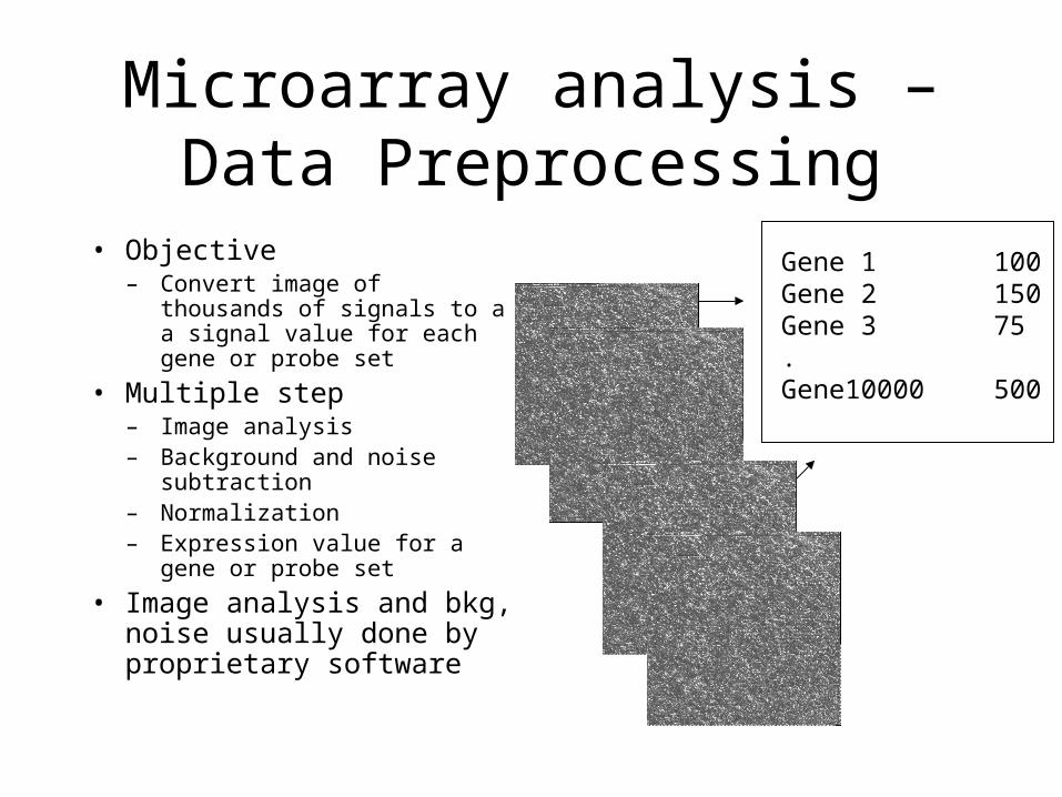
Microarray analysis – Data Preprocessing

• Objective– Convert image of thousands of

signals to a a signal value for each gene or probe set

• Multiple step– Image analysis– Background and noise

subtraction– Normalization– Expression value for a gene or

probe set

• Image analysis and bkg, noise usually done by proprietary software

Gene 1 100Gene 2 150Gene 3 75.Gene10000 500

Normalization• Corrects for variation in

hybridization etc• Assumption that no

global change in gene expression

• Without normalization– Intensity value for gene

will be lower on Chip B– Many genes will appear to

be downregulated when in reality they are not

Gene 1 100Gene 2 150Gene 3 75.Gene10000 500

507532

250

Treated Control

Data Analysis

• Part 2- Data analysis– Class discovery

– Class comparison

– Class prediction

– Biological annotation

– Pathway analysis

Class Discovery• Objective?

– Can data tell us which classes are similar?– Are there subgroups?– Do T-ALL, T-LL, B-ALL fall into distinct groups?

• Methods– Hierarchical clustering– K-means, SOM etc– These are Unsupervised Methods

• Class Ids are not known to the algorithm– For example, does not know which one is cancer or non cancer– Do the expression values differentiate, does it discover new classes

Hierarchical Clustering

• Eisen Cluster and Treeview• Import data• Filter

– Filter or not to filter, %P calls, SD etc• Accept filter

• Adjust data– Log transform (important), center,

normalize• Clustering

– Cluster array or genes– Gene computationally intensive– Choose distance metric

• .cdt file created– Open with Treeview

Experimental Design – Very important!!!

• Sample size– How many samples in test and

control• Will depend on many factors

such as whether tissue culture or tissue sample

• Power analysis

• Replicates– Technical v biological

• Biological replicates is more important for more heterogenous samples Need replicates for statistical analysis

• To pool or not to pool– Depends on objective

• Sample acquistion or extraction– Laser captered or gross

dissected

• All experimental steps from sample acquisition to hybridization– Microarray experiments are

very expensive. So, plan experiments carefully

Venn Diagramhttp://www.pangloss.com/seidel/Protocols/venn.cgi

http://ncrr.pnl.gov/software/VennDiagramPlotter.stm

Conclusion• Other analysis

– Class prediction– Gene list from class comparison can be used in

pathway analysis– HSLS pathway workshops on Ingenuity, DAVID,

Pathway Architect– Future:

• Integrate expression data with other data such as snp or microRNA

• GEO has some data analysis features

End Theory I

• 5 min Mindmapping

• 10 min Break

Theory II

Microarrays

• Gene Expression:– We see difference between cells because of

differential gene expression,– Gene is expressed by transcribing DNA intosingle-

stranded mRNA,– mRNA is later translated into a protein,– Microarrays measure the level of mRNA

expression

Microarrays

• Gene Expression:– mRNA expression represents dynamic aspects of

cell,– mRNA is isolated and labeled using a fluorescent

material,– mRNA is hybridized to the target; level of

hybridization corresponds to light emission which is measured with a laser

Microarrays

Microarrays

Microarrays

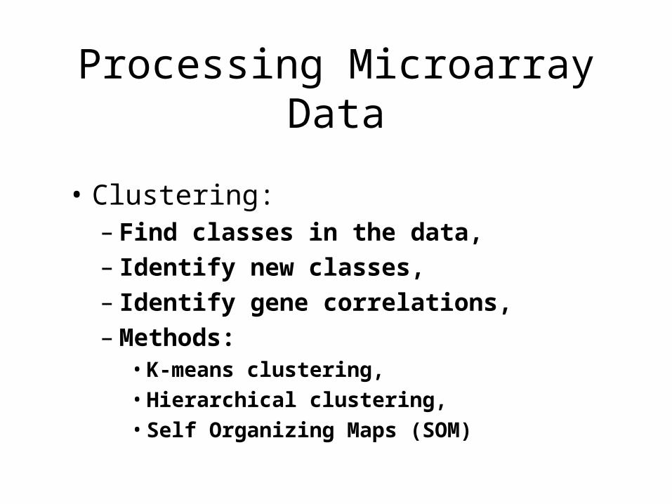
Processing Microarray Data

• Differentiating gene expression:

– R = G not differentiated

– R > G up-regulated

– R < G down regulated

Processing Microarray Data

• Problems:– Extract data from microarrays,– Analyze the meaning of the multiple arrays.

Processing Microarray Data

Processing Microarray Data

• Problems:– Extract data from microarrays,– Analyze the meaning of the multiple arrays.

Processing Microarray Data

• Microarray data:

Processing Microarray Data

• Clustering:– Find classes in the data,– Identify new classes,– Identify gene correlations,– Methods:

• K-means clustering,

• Hierarchical clustering,

• Self Organizing Maps (SOM)

Processing Microarray Data

• Distance Measures:– Euclidean Distance:

– Manhattan Distance:

Processing Microarray Data

• K-means Clustering:– Break the data into K clusters,– Start with random partitioning,– Improve it by iterating.

Processing Microarray Data

• Agglomerative Hierarchical Clustering:

Processing Microarray Data

• Self-Organizing Feature Maps:– by Teuvo Kohonen, – a data visualization technique which helps to

understand high dimensional data by reducing the dimensions of data to a map.

Processing Microarray Data

• Self-Organizing Feature Maps:– humans simply cannot visualize high dimensional

data as is,– SOM help us understand this high dimensional

data.

Processing Microarray Data

• Self-Organizing Feature Maps:– Based on competitive learning,– SOM helps us by producing a map of usually 1 or 2

dimensions,– SOM plot the similarities of the data by grouping– similar data items together.

Processing Microarray Data

• Self-Organizing Feature Maps:

Processing Microarray Data

• Self-Organizing Feature Maps: Input vector, synaptic weight vector

x = [x1, x2, …, xm]T

wj=[wj1, wj2, …, wjm]T, j = 1, 2,3, l

Best matching, winning neuroni(x) = arg min ||x-wj||, j =1,2,3,..,l

Weights wi are updated.

Figure 2. Output map containing the distributions of genes from the alpha30 database.

Chavez-Alvarez R, Chavoya A, Mendez-Vazquez A (2014) Discovery of Possible Gene Relationships through the Application of Self-Organizing Maps to DNA Microarray Databases. PLoS ONE 9(4): e93233. doi:10.1371/journal.pone.0093233http://www.plosone.org/article/info:doi/10.1371/journal.pone.0093233

Figure 5. Color-coded output maps representing the final weight of neurons from the samples of the alpha30 database.

Chavez-Alvarez R, Chavoya A, Mendez-Vazquez A (2014) Discovery of Possible Gene Relationships through the Application of Self-Organizing Maps to DNA Microarray Databases. PLoS ONE 9(4): e93233. doi:10.1371/journal.pone.0093233http://www.plosone.org/article/info:doi/10.1371/journal.pone.0093233

End Theory II

• 5 min mindmapping

• 10 min break

Practice I

Microarray

• http://www.biolab.si/supp/bi-visprog/dicty/dictyExample.htm

• Use the data as described on the page