introduction to dynamic systems (network mathematics graduate

Introduction to Dynamic Systems

(Network Mathematics Graduate Programme)

Martin Corless

School of Aeronautics & AstronauticsPurdue University

West Lafayette, [email protected]

July 14, 2011

Contents

I Representation of Dynamical Systems vii

1 Introduction 11.1 Ingredients . . . . . . . . . . . . . . . . . . . . . . . . . . . . . . . . . . . . . 41.2 Some notation . . . . . . . . . . . . . . . . . . . . . . . . . . . . . . . . . . . 41.3 MATLAB . . . . . . . . . . . . . . . . . . . . . . . . . . . . . . . . . . . . . 4

2 State space representation of dynamical systems 52.1 Linear examples . . . . . . . . . . . . . . . . . . . . . . . . . . . . . . . . . . 5

2.1.1 A first example . . . . . . . . . . . . . . . . . . . . . . . . . . . . . . 52.1.2 The unattached mass . . . . . . . . . . . . . . . . . . . . . . . . . . . 62.1.3 Spring-mass-damper . . . . . . . . . . . . . . . . . . . . . . . . . . . 62.1.4 A simple structure . . . . . . . . . . . . . . . . . . . . . . . . . . . . 7

2.2 Nonlinear examples . . . . . . . . . . . . . . . . . . . . . . . . . . . . . . . . 82.2.1 A first nonlinear system . . . . . . . . . . . . . . . . . . . . . . . . . 82.2.2 Planar pendulum . . . . . . . . . . . . . . . . . . . . . . . . . . . . . 92.2.3 Attitude dynamics of a rigid body . . . . . . . . . . . . . . . . . . . . 92.2.4 Body in central force motion . . . . . . . . . . . . . . . . . . . . . . . 102.2.5 Double pendulum on cart . . . . . . . . . . . . . . . . . . . . . . . . 112.2.6 Two-link robotic manipulator . . . . . . . . . . . . . . . . . . . . . . 12

2.3 Discrete-time examples . . . . . . . . . . . . . . . . . . . . . . . . . . . . . . 132.3.1 The discrete unattached mass . . . . . . . . . . . . . . . . . . . . . . 132.3.2 Additive increase multiplicative decrease (AIMD) algorithm for re-

source allocation . . . . . . . . . . . . . . . . . . . . . . . . . . . . . 142.4 General representation . . . . . . . . . . . . . . . . . . . . . . . . . . . . . . 16

2.4.1 Continuous-time . . . . . . . . . . . . . . . . . . . . . . . . . . . . . 162.4.2 Discrete-time . . . . . . . . . . . . . . . . . . . . . . . . . . . . . . . 192.4.3 Exercises . . . . . . . . . . . . . . . . . . . . . . . . . . . . . . . . . . 21

2.5 Vectors . . . . . . . . . . . . . . . . . . . . . . . . . . . . . . . . . . . . . . . 232.5.1 Vector spaces and IRn . . . . . . . . . . . . . . . . . . . . . . . . . . 232.5.2 IR2 and pictures . . . . . . . . . . . . . . . . . . . . . . . . . . . . . . 252.5.3 Derivatives . . . . . . . . . . . . . . . . . . . . . . . . . . . . . . . . 262.5.4 MATLAB . . . . . . . . . . . . . . . . . . . . . . . . . . . . . . . . . 26

2.6 Vector representation of dynamical systems . . . . . . . . . . . . . . . . . . . 272.7 Solutions and equilibrium states : continuous-time . . . . . . . . . . . . . . 30

2.7.1 Equilibrium states . . . . . . . . . . . . . . . . . . . . . . . . . . . . 30

iii

2.7.2 Exercises . . . . . . . . . . . . . . . . . . . . . . . . . . . . . . . . . . 322.7.3 Controlled equilibrium states . . . . . . . . . . . . . . . . . . . . . . 33

2.8 Solutions and equilibrium states: discrete-time . . . . . . . . . . . . . . . . . 332.8.1 Equilibrium states . . . . . . . . . . . . . . . . . . . . . . . . . . . . 332.8.2 Controlled equilibrium states . . . . . . . . . . . . . . . . . . . . . . 35

2.9 Numerical simulation . . . . . . . . . . . . . . . . . . . . . . . . . . . . . . . 362.9.1 MATLAB . . . . . . . . . . . . . . . . . . . . . . . . . . . . . . . . . 362.9.2 Simulink . . . . . . . . . . . . . . . . . . . . . . . . . . . . . . . . . . 37

2.10 Exercises . . . . . . . . . . . . . . . . . . . . . . . . . . . . . . . . . . . . . . 38

3 Linear time-invariant (LTI) systems 413.1 Matrices . . . . . . . . . . . . . . . . . . . . . . . . . . . . . . . . . . . . . . 413.2 Linear time-invariant systems . . . . . . . . . . . . . . . . . . . . . . . . . . 46

3.2.1 Continuous-time . . . . . . . . . . . . . . . . . . . . . . . . . . . . . 463.2.2 Discrete-time . . . . . . . . . . . . . . . . . . . . . . . . . . . . . . . 47

3.3 Linearization about an equilibrium solution . . . . . . . . . . . . . . . . . . 483.3.1 Derivative as a matrix . . . . . . . . . . . . . . . . . . . . . . . . . . 483.3.2 Linearization of continuous-time systems . . . . . . . . . . . . . . . . 493.3.3 Implicit linearization . . . . . . . . . . . . . . . . . . . . . . . . . . . 523.3.4 Linearization of discrete-time systems . . . . . . . . . . . . . . . . . . 55

4 Transfer functions 594.1 ←− Transfer functions ←− . . . . . . . . . . . . . . . . . . . . . . . . . . . 59

4.1.1 The Laplace transform . . . . . . . . . . . . . . . . . . . . . . . . . . 594.1.2 Transfer functions . . . . . . . . . . . . . . . . . . . . . . . . . . . . . 604.1.3 Poles and zeros . . . . . . . . . . . . . . . . . . . . . . . . . . . . . . 674.1.4 Discrete-time . . . . . . . . . . . . . . . . . . . . . . . . . . . . . . . 714.1.5 Exercises . . . . . . . . . . . . . . . . . . . . . . . . . . . . . . . . . . 71

4.2 Some transfer function properties . . . . . . . . . . . . . . . . . . . . . . . . 734.2.1 Power series expansion and Markov parameters . . . . . . . . . . . . 734.2.2 More properties* . . . . . . . . . . . . . . . . . . . . . . . . . . . . . 73

4.3 State space realization of transfer functions . . . . . . . . . . . . . . . . . . . 754.4 Realization of SISO transfer functions . . . . . . . . . . . . . . . . . . . . . . 76

4.4.1 Controllable canonical form realization . . . . . . . . . . . . . . . . . 764.4.2 Observable canonical form realization . . . . . . . . . . . . . . . . . . 77

4.5 Realization of MIMO systems . . . . . . . . . . . . . . . . . . . . . . . . . . 804.5.1 Controllable realizations . . . . . . . . . . . . . . . . . . . . . . . . . 804.5.2 Observable realizations . . . . . . . . . . . . . . . . . . . . . . . . . . 834.5.3 Alternative realizations∗ . . . . . . . . . . . . . . . . . . . . . . . . . 84

II System Behavior and Stability 89

5 Behavior of (LTI) systems : I 915.1 Initial stuff . . . . . . . . . . . . . . . . . . . . . . . . . . . . . . . . . . . . 91

5.1.1 Continuous-time . . . . . . . . . . . . . . . . . . . . . . . . . . . . . 915.1.2 Discrete-time . . . . . . . . . . . . . . . . . . . . . . . . . . . . . . . 92

5.2 Scalar systems . . . . . . . . . . . . . . . . . . . . . . . . . . . . . . . . . . . 935.2.1 Continuous-time . . . . . . . . . . . . . . . . . . . . . . . . . . . . . 935.2.2 First order complex and second order real. . . . . . . . . . . . . . . . 945.2.3 DT . . . . . . . . . . . . . . . . . . . . . . . . . . . . . . . . . . . . . 96

5.3 Eigenvalues and eigenvectors . . . . . . . . . . . . . . . . . . . . . . . . . . . 975.3.1 Real A . . . . . . . . . . . . . . . . . . . . . . . . . . . . . . . . . . . 1005.3.2 MATLAB . . . . . . . . . . . . . . . . . . . . . . . . . . . . . . . . . 1015.3.3 Companion matrices . . . . . . . . . . . . . . . . . . . . . . . . . . . 102

5.4 Behavior of continuous-time systems . . . . . . . . . . . . . . . . . . . . . . 1035.4.1 System significance of eigenvectors and eigenvalues . . . . . . . . . . 1035.4.2 Solutions for nondefective matrices . . . . . . . . . . . . . . . . . . . 1095.4.3 Defective matrices and generalized eigenvectors . . . . . . . . . . . . 110

5.5 Behavior of discrete-time systems . . . . . . . . . . . . . . . . . . . . . . . . 1155.5.1 System significance of eigenvectors and eigenvalues . . . . . . . . . . 1155.5.2 All solutions for nondefective matrices . . . . . . . . . . . . . . . . . 1165.5.3 Some solutions for defective matrices . . . . . . . . . . . . . . . . . . 116

5.6 Similarity transformations . . . . . . . . . . . . . . . . . . . . . . . . . . . . 1185.7 Hotel California . . . . . . . . . . . . . . . . . . . . . . . . . . . . . . . . . . 123

5.7.1 Invariant subspaces . . . . . . . . . . . . . . . . . . . . . . . . . . . . 1235.7.2 More on invariant subspaces∗ . . . . . . . . . . . . . . . . . . . . . . 124

5.8 Diagonalizable systems . . . . . . . . . . . . . . . . . . . . . . . . . . . . . . 1265.8.1 Diagonalizable matrices . . . . . . . . . . . . . . . . . . . . . . . . . 1265.8.2 Diagonalizable continuous-time systems . . . . . . . . . . . . . . . . . 1285.8.3 Diagonalizable DT systems . . . . . . . . . . . . . . . . . . . . . . . . 130

5.9 Real Jordan form for real diagonalizable systems∗ . . . . . . . . . . . . . . . 1325.9.1 CT systems . . . . . . . . . . . . . . . . . . . . . . . . . . . . . . . . 133

5.10 Diagonalizable second order systems . . . . . . . . . . . . . . . . . . . . . . 1335.10.1 State plane portraits for CT systems . . . . . . . . . . . . . . . . . . 134

5.11 Exercises . . . . . . . . . . . . . . . . . . . . . . . . . . . . . . . . . . . . . . 134

6 eAt 1416.1 State transition matrix . . . . . . . . . . . . . . . . . . . . . . . . . . . . . . 141

6.1.1 Continuous time . . . . . . . . . . . . . . . . . . . . . . . . . . . . . 1416.1.2 Discrete time . . . . . . . . . . . . . . . . . . . . . . . . . . . . . . . 143

6.2 Polynomials of a square matrix . . . . . . . . . . . . . . . . . . . . . . . . . 1446.2.1 Polynomials of a matrix . . . . . . . . . . . . . . . . . . . . . . . . . 1446.2.2 Cayley-Hamilton Theorem . . . . . . . . . . . . . . . . . . . . . . . . 145

6.3 Functions of a square matrix . . . . . . . . . . . . . . . . . . . . . . . . . . . 1476.3.1 The matrix exponential: eA . . . . . . . . . . . . . . . . . . . . . . . 1506.3.2 Other matrix functions . . . . . . . . . . . . . . . . . . . . . . . . . . 150

6.4 The state transition matrix: eAt . . . . . . . . . . . . . . . . . . . . . . . . . 1516.5 Computation of eAt . . . . . . . . . . . . . . . . . . . . . . . . . . . . . . . . 152

6.5.1 MATLAB . . . . . . . . . . . . . . . . . . . . . . . . . . . . . . . . . 152

6.5.2 Numerical simulation . . . . . . . . . . . . . . . . . . . . . . . . . . . 152

6.5.3 Jordan form . . . . . . . . . . . . . . . . . . . . . . . . . . . . . . . . 152

6.5.4 Laplace style . . . . . . . . . . . . . . . . . . . . . . . . . . . . . . . 152

6.6 Sampled-data systems . . . . . . . . . . . . . . . . . . . . . . . . . . . . . . 154

6.7 Exercises . . . . . . . . . . . . . . . . . . . . . . . . . . . . . . . . . . . . . . 155

7 Stability and boundedness 159

7.1 Boundedness of solutions . . . . . . . . . . . . . . . . . . . . . . . . . . . . . 159

7.2 Stability of equilibrium states . . . . . . . . . . . . . . . . . . . . . . . . . . 162

7.3 Asymptotic stability . . . . . . . . . . . . . . . . . . . . . . . . . . . . . . . 164

7.3.1 Global asymptotic stability . . . . . . . . . . . . . . . . . . . . . . . 164

7.3.2 Asymptotic stability . . . . . . . . . . . . . . . . . . . . . . . . . . . 164

7.4 Exponential stability . . . . . . . . . . . . . . . . . . . . . . . . . . . . . . . 166

7.5 LTI systems . . . . . . . . . . . . . . . . . . . . . . . . . . . . . . . . . . . . 167

7.6 Linearization and stability . . . . . . . . . . . . . . . . . . . . . . . . . . . . 170

8 Stability and boundedness: discrete time 173

8.1 Boundedness of solutions . . . . . . . . . . . . . . . . . . . . . . . . . . . . . 173

8.2 Stability of equilibrium states . . . . . . . . . . . . . . . . . . . . . . . . . . 174


8.3.1 Global asymptotic stability . . . . . . . . . . . . . . . . . . . . . . . 175

8.3.2 Asymptotic stability . . . . . . . . . . . . . . . . . . . . . . . . . . . 175


8.5 LTI systems . . . . . . . . . . . . . . . . . . . . . . . . . . . . . . . . . . . . 177

8.6 Linearization and stability . . . . . . . . . . . . . . . . . . . . . . . . . . . . 178

9 Basic Lyapunov theory 179

9.1 Stability . . . . . . . . . . . . . . . . . . . . . . . . . . . . . . . . . . . . . . 181

9.1.1 Locally positive definite functions . . . . . . . . . . . . . . . . . . . . 181

9.1.2 A stability result . . . . . . . . . . . . . . . . . . . . . . . . . . . . . 183


9.3 Boundedness . . . . . . . . . . . . . . . . . . . . . . . . . . . . . . . . . . . 189

9.3.1 Radially unbounded functions . . . . . . . . . . . . . . . . . . . . . . 189

9.3.2 A boundedness result . . . . . . . . . . . . . . . . . . . . . . . . . . . 189

9.4 Global asymptotic stability . . . . . . . . . . . . . . . . . . . . . . . . . . . . 192

9.4.1 Positive definite functions . . . . . . . . . . . . . . . . . . . . . . . . 192

9.4.2 A result on global asymptotic stability . . . . . . . . . . . . . . . . . 193


9.5.1 Global exponential stability . . . . . . . . . . . . . . . . . . . . . . . 196

9.5.2 Proof of theorem ?? . . . . . . . . . . . . . . . . . . . . . . . . . . . 197

9.5.3 Exponential stability . . . . . . . . . . . . . . . . . . . . . . . . . . . 197

9.5.4 A special class of GES systems . . . . . . . . . . . . . . . . . . . . . 199

9.5.5 Summary . . . . . . . . . . . . . . . . . . . . . . . . . . . . . . . . . 201

10 Basic Lyapunov theory: discrete time* 20310.1 Stability . . . . . . . . . . . . . . . . . . . . . . . . . . . . . . . . . . . . . . 20410.2 Asymptotic stability . . . . . . . . . . . . . . . . . . . . . . . . . . . . . . . 20510.3 Boundedness . . . . . . . . . . . . . . . . . . . . . . . . . . . . . . . . . . . 20610.4 Global asymptotic stability . . . . . . . . . . . . . . . . . . . . . . . . . . . . 20710.5 Exponential stability . . . . . . . . . . . . . . . . . . . . . . . . . . . . . . . 208

11 Lyapunov theory for linear time-invariant systems 21111.1 Positive and negative (semi)definite matrices . . . . . . . . . . . . . . . . . . 211

11.1.1 Definite matrices . . . . . . . . . . . . . . . . . . . . . . . . . . . . . 21111.1.2 Semi-definite matrices* . . . . . . . . . . . . . . . . . . . . . . . . . . 212

11.2 Lyapunov theory . . . . . . . . . . . . . . . . . . . . . . . . . . . . . . . . . 21411.2.1 Asymptotic stability results . . . . . . . . . . . . . . . . . . . . . . . 21411.2.2 MATLAB. . . . . . . . . . . . . . . . . . . . . . . . . . . . . . . . . . 21811.2.3 Stability results* . . . . . . . . . . . . . . . . . . . . . . . . . . . . . 219

11.3 Mechanical systems* . . . . . . . . . . . . . . . . . . . . . . . . . . . . . . . 22111.4 Rates of convergence for linear systems* . . . . . . . . . . . . . . . . . . . . 22411.5 Linearization and exponential stability . . . . . . . . . . . . . . . . . . . . . 225

III Input-Output Properties 227

12 Input output response 22912.1 Response of continuous-time systems . . . . . . . . . . . . . . . . . . . . . . 229

12.1.1 State response and the convolution integral . . . . . . . . . . . . . . . 22912.1.2 Output response . . . . . . . . . . . . . . . . . . . . . . . . . . . . . 231

12.2 Discretization and zero-order hold . . . . . . . . . . . . . . . . . . . . . . . . 23512.2.1 Input-output discretization . . . . . . . . . . . . . . . . . . . . . . . . 238

12.3 Response of discrete-time systems* . . . . . . . . . . . . . . . . . . . . . . . 23912.3.1 State response and the convolution sum . . . . . . . . . . . . . . . . 23912.3.2 Input-output response and the pulse response matrix . . . . . . . . . 239

13 Observability 24313.1 Observability . . . . . . . . . . . . . . . . . . . . . . . . . . . . . . . . . . . 24313.2 Main result . . . . . . . . . . . . . . . . . . . . . . . . . . . . . . . . . . . . 24413.3 Development of main result . . . . . . . . . . . . . . . . . . . . . . . . . . . 25013.4 The unobservable subspace . . . . . . . . . . . . . . . . . . . . . . . . . . . . 25313.5 Unobservable modes . . . . . . . . . . . . . . . . . . . . . . . . . . . . . . . 255

13.5.1 PBH Test . . . . . . . . . . . . . . . . . . . . . . . . . . . . . . . . . 25613.5.2 Existence of unobservable modes* . . . . . . . . . . . . . . . . . . . . 25913.5.3 A nice transformation* . . . . . . . . . . . . . . . . . . . . . . . . . . 260

13.6 Observability grammians* . . . . . . . . . . . . . . . . . . . . . . . . . . . . 26513.6.1 Infinite time observability grammian . . . . . . . . . . . . . . . . . . 268

13.7 Discrete time . . . . . . . . . . . . . . . . . . . . . . . . . . . . . . . . . . . 27013.7.1 Main observability result . . . . . . . . . . . . . . . . . . . . . . . . . 270

13.8 Exercises . . . . . . . . . . . . . . . . . . . . . . . . . . . . . . . . . . . . . . 271

14 Controllability 27514.1 Controllability . . . . . . . . . . . . . . . . . . . . . . . . . . . . . . . . . . . 27514.2 Main controllability result . . . . . . . . . . . . . . . . . . . . . . . . . . . . 27614.3 The controllable subspace . . . . . . . . . . . . . . . . . . . . . . . . . . . . 28014.4 Proof of the controllable subspace lemma* . . . . . . . . . . . . . . . . . . . 284

14.4.1 Finite time controllability grammian . . . . . . . . . . . . . . . . . . 28414.4.2 Proof of the controllable subspace lemma . . . . . . . . . . . . . . . . 286

14.5 Uncontrollable modes . . . . . . . . . . . . . . . . . . . . . . . . . . . . . . . 28714.5.1 Eigenvectors revisited: left eigenvectors . . . . . . . . . . . . . . . . . 28714.5.2 Uncontrollable eigenvalues and modes . . . . . . . . . . . . . . . . . . 28914.5.3 Existence of uncontrollable modes* . . . . . . . . . . . . . . . . . . . 28914.5.4 A nice transformation* . . . . . . . . . . . . . . . . . . . . . . . . . . 291

14.6 PBH test . . . . . . . . . . . . . . . . . . . . . . . . . . . . . . . . . . . . . 29514.6.1 PBH test for uncontrollable eigenvalues . . . . . . . . . . . . . . . . . 29514.6.2 PBH controllability test . . . . . . . . . . . . . . . . . . . . . . . . . 297

14.7 Other characterizations of controllability* . . . . . . . . . . . . . . . . . . . 29814.7.1 Infinite time controllability grammian . . . . . . . . . . . . . . . . . . 298

14.8 Controllability, observability, and duality . . . . . . . . . . . . . . . . . . . . 29914.9 Discrete-time . . . . . . . . . . . . . . . . . . . . . . . . . . . . . . . . . . . 300

14.9.1 Main controllability theorem . . . . . . . . . . . . . . . . . . . . . . . 300

IV Control Design 301

15 Stabilizability and state feedback 30315.1 Stabilizability and state feedback . . . . . . . . . . . . . . . . . . . . . . . . 30315.2 Eigenvalue placement (pole placement) by state feedback . . . . . . . . . . . 304

15.2.1 Single input systems . . . . . . . . . . . . . . . . . . . . . . . . . . . 30515.2.2 Multi-input systems . . . . . . . . . . . . . . . . . . . . . . . . . . . 310

15.3 Uncontrollable eigenvalues (you can’t touch them) . . . . . . . . . . . . . . . 31215.4 Controllable canonical form . . . . . . . . . . . . . . . . . . . . . . . . . . . 315

15.4.1 Transformation to controllable canonical form∗ . . . . . . . . . . . . . 31615.4.2 Eigenvalue placement by state feedback∗ . . . . . . . . . . . . . . . . 319

15.5 Discrete-time systems . . . . . . . . . . . . . . . . . . . . . . . . . . . . . . . 32115.5.1 Dead beat controllers . . . . . . . . . . . . . . . . . . . . . . . . . . . 321

15.6 Stabilization of nonlinear systems . . . . . . . . . . . . . . . . . . . . . . . . 32215.6.1 Continuous-time controllers . . . . . . . . . . . . . . . . . . . . . . . 32215.6.2 Discrete-time controllers . . . . . . . . . . . . . . . . . . . . . . . . . 322

15.7 Appendix . . . . . . . . . . . . . . . . . . . . . . . . . . . . . . . . . . . . . 326

16 Detectability and observers 32916.1 Observers, state estimators and detectability . . . . . . . . . . . . . . . . . 32916.2 Eigenvalue placement for estimation error dynamics . . . . . . . . . . . . . . 331

16.3 Unobservable modes (you can’t see them) . . . . . . . . . . . . . . . . . . . . 33216.4 Observable canonical form* . . . . . . . . . . . . . . . . . . . . . . . . . . . 33316.5 Discrete-time systems . . . . . . . . . . . . . . . . . . . . . . . . . . . . . . . 334

17 Climax: output feedback controllers 33717.1 Memoryless (static) output feedback . . . . . . . . . . . . . . . . . . . . . . 33717.2 Dynamic output feedback . . . . . . . . . . . . . . . . . . . . . . . . . . . . 33817.3 Observer based controllers . . . . . . . . . . . . . . . . . . . . . . . . . . . . 34017.4 Discrete-time systems . . . . . . . . . . . . . . . . . . . . . . . . . . . . . . . 343

17.4.1 Memoryless output feedback . . . . . . . . . . . . . . . . . . . . . . . 34317.4.2 Dynamic output feedback . . . . . . . . . . . . . . . . . . . . . . . . 34317.4.3 Observer based controllers . . . . . . . . . . . . . . . . . . . . . . . . 344

18 Constant output tracking in the presence of constant disturbances 34718.1 Zeros . . . . . . . . . . . . . . . . . . . . . . . . . . . . . . . . . . . . . . . . 347

18.1.1 A state space characterization of zeros . . . . . . . . . . . . . . . . . 34718.2 Tracking and disturbance rejection with state feedback . . . . . . . . . . . . 350

18.2.1 Nonrobust control . . . . . . . . . . . . . . . . . . . . . . . . . . . . . 35218.2.2 Robust controller . . . . . . . . . . . . . . . . . . . . . . . . . . . . . 352

18.3 Measured Output Feedback Control . . . . . . . . . . . . . . . . . . . . . . . 35518.3.1 Observer based controllers . . . . . . . . . . . . . . . . . . . . . . . . 357

19 Lyapunov revisited* 36119.1 Stability, observability, and controllability . . . . . . . . . . . . . . . . . . . 36119.2 A simple stabilizing controller . . . . . . . . . . . . . . . . . . . . . . . . . . 365

20 Performance* 36720.1 The L2 norm . . . . . . . . . . . . . . . . . . . . . . . . . . . . . . . . . . . 367

20.1.1 The rms value of a signal . . . . . . . . . . . . . . . . . . . . . . . . . 36720.1.2 The L2 norm of a time-varying matrix . . . . . . . . . . . . . . . . . 368

20.2 The H2 norm of an LTI system . . . . . . . . . . . . . . . . . . . . . . . . . 36820.3 Computation of the H2 norm . . . . . . . . . . . . . . . . . . . . . . . . . . 369

21 Linear quadratic regulators (LQR) 37321.1 The linear quadratic optimal control problem . . . . . . . . . . . . . . . . . 37321.2 The algebraic Riccati equation (ARE) . . . . . . . . . . . . . . . . . . . . . 37521.3 Linear state feedback controllers . . . . . . . . . . . . . . . . . . . . . . . . . 37621.4 Infimal cost* . . . . . . . . . . . . . . . . . . . . . . . . . . . . . . . . . . . . 377

21.4.1 Reduced cost stabilizing controllers. . . . . . . . . . . . . . . . . . . . 37721.4.2 Cost reducing algorithm . . . . . . . . . . . . . . . . . . . . . . . . . 37721.4.3 Infimal cost . . . . . . . . . . . . . . . . . . . . . . . . . . . . . . . . 380

21.5 Optimal stabilizing controllers . . . . . . . . . . . . . . . . . . . . . . . . . . 38321.5.1 Existence of stabilizing solutions to the ARE . . . . . . . . . . . . . . 385

21.6 Summary . . . . . . . . . . . . . . . . . . . . . . . . . . . . . . . . . . . . . 38621.7 MATLAB . . . . . . . . . . . . . . . . . . . . . . . . . . . . . . . . . . . . . 389

21.8 Minimum energy controllers . . . . . . . . . . . . . . . . . . . . . . . . . . . 39021.9 H2 optimal controllers* . . . . . . . . . . . . . . . . . . . . . . . . . . . . . . 39221.10Exercises . . . . . . . . . . . . . . . . . . . . . . . . . . . . . . . . . . . . . . 39421.11Appendix . . . . . . . . . . . . . . . . . . . . . . . . . . . . . . . . . . . . . 395

21.11.1Proof of fact 1 . . . . . . . . . . . . . . . . . . . . . . . . . . . . . . . 395

22 LQG controllers 39722.1 LQ observer . . . . . . . . . . . . . . . . . . . . . . . . . . . . . . . . . . . . 39722.2 LQG controllers . . . . . . . . . . . . . . . . . . . . . . . . . . . . . . . . . . 39822.3 H2 Optimal controllers* . . . . . . . . . . . . . . . . . . . . . . . . . . . . . 399

22.3.1 LQ observers . . . . . . . . . . . . . . . . . . . . . . . . . . . . . . . 39922.3.2 LQG controllers . . . . . . . . . . . . . . . . . . . . . . . . . . . . . . 400

23 Systems with inputs and outputs: II* 40123.1 Minimal realizations . . . . . . . . . . . . . . . . . . . . . . . . . . . . . . . 40123.2 Exercises . . . . . . . . . . . . . . . . . . . . . . . . . . . . . . . . . . . . . . 402

24 Time-varying systems* 40324.1 Linear time-varying systems (LTVs) . . . . . . . . . . . . . . . . . . . . . . . 403

24.1.1 Linearization about time-varying trajectories . . . . . . . . . . . . . . 40324.2 The state transition matrix . . . . . . . . . . . . . . . . . . . . . . . . . . . 40424.3 Stability . . . . . . . . . . . . . . . . . . . . . . . . . . . . . . . . . . . . . . 40524.4 Systems with inputs and outputs . . . . . . . . . . . . . . . . . . . . . . . . 40624.5 DT . . . . . . . . . . . . . . . . . . . . . . . . . . . . . . . . . . . . . . . . . 406

25 Appendix A: Complex stuff 40925.1 Complex numbers . . . . . . . . . . . . . . . . . . . . . . . . . . . . . . . . . 409

25.1.1 Complex functions . . . . . . . . . . . . . . . . . . . . . . . . . . . . 41125.2 Complex vectors and Cn . . . . . . . . . . . . . . . . . . . . . . . . . . . . . 41225.3 Complex matrices and Cm×n . . . . . . . . . . . . . . . . . . . . . . . . . . . 412

26 Appendix B: Norms 41526.1 The Euclidean norm . . . . . . . . . . . . . . . . . . . . . . . . . . . . . . . 415

27 Appendix C: Some linear algebra 41727.1 Linear equations . . . . . . . . . . . . . . . . . . . . . . . . . . . . . . . . . 41727.2 Subspaces . . . . . . . . . . . . . . . . . . . . . . . . . . . . . . . . . . . . . 42427.3 Basis . . . . . . . . . . . . . . . . . . . . . . . . . . . . . . . . . . . . . . . . 425

27.3.1 Span (not Spam) . . . . . . . . . . . . . . . . . . . . . . . . . . . . . 42527.3.2 Linear independence . . . . . . . . . . . . . . . . . . . . . . . . . . . 42627.3.3 Basis . . . . . . . . . . . . . . . . . . . . . . . . . . . . . . . . . . . . 431

27.4 Range and null space of a matrix . . . . . . . . . . . . . . . . . . . . . . . . 43227.4.1 Null space . . . . . . . . . . . . . . . . . . . . . . . . . . . . . . . . . 43227.4.2 Range . . . . . . . . . . . . . . . . . . . . . . . . . . . . . . . . . . . 43427.4.3 Solving linear equations revisited . . . . . . . . . . . . . . . . . . . . 437

27.5 Coordinate transformations . . . . . . . . . . . . . . . . . . . . . . . . . . . 440

27.5.1 Coordinate transformations and linear maps . . . . . . . . . . . . . . 44027.5.2 The structure of a linear map . . . . . . . . . . . . . . . . . . . . . . 442

28 Appendix D: Inner products 44528.1 The usual scalar product on IRn and Cn . . . . . . . . . . . . . . . . . . . . 44528.2 Orthogonality . . . . . . . . . . . . . . . . . . . . . . . . . . . . . . . . . . . 446

28.2.1 Orthonormal basis . . . . . . . . . . . . . . . . . . . . . . . . . . . . 44728.3 Hermitian matrices . . . . . . . . . . . . . . . . . . . . . . . . . . . . . . . . 44928.4 Positive and negative (semi)definite matrices . . . . . . . . . . . . . . . . . . 450

28.4.1 Quadratic forms . . . . . . . . . . . . . . . . . . . . . . . . . . . . . . 45028.4.2 Definite matrices . . . . . . . . . . . . . . . . . . . . . . . . . . . . . 45128.4.3 Semi-definite matrices . . . . . . . . . . . . . . . . . . . . . . . . . . 452

28.5 Singular value decomposition . . . . . . . . . . . . . . . . . . . . . . . . . . 453

xi

Preface

These notes were developed to accompany the corresponding course in the Network Math-ematics Graduate Programme at the Hamilton Institute. The purpose of the course is tointroduce some basic concepts and results in the analysis and control of linear and nonlin-ear dynamical systems. There is a lot more material in these notes than can be covered intwenty hours. However, the extra material should prove useful to the student who wants topursue a specific topic in more depth. Sections marked with an asterisk will not be covered.Although proofs are given for most of the results presented here, they will not be covered inthe course.

xiii

Part I

Representation of Dynamical Systems

xv

Chapter 1

Introduction

The purpose of this course is to introduce some basic concepts and tools which are usefulin the analysis and control of dynamical systems. The concept of a dynamical system isvery general; it refers to anything which evolves with time. A communication network is adynamical system. Vehicles (aircraft, spacecraft, motorcycles, cars) are dynamical systems.Other engineering examples of dynamical systems include, metal cutting machines such aslathes and milling machines, robots, chemical plants, and electrical circuits. Even civilengineering structures such as bridges and skyscrapers are examples; think of a structuresubject to strong winds or an earthquake. The concept of a dynamical system is not restrictedto engineering; non-engineering examples include plants, animals, yourself, and the economy.

A system interacts with its environment via inputs and outputs. Inputs can be consideredto be exerted on the system by the environment whereas outputs are exerted by the systemon the environment. Inputs are usually divided into control inputs and disturbance inputs.In an aircraft, the deflection of a control surface such as an elevator would be considered acontrol input; a wind gust would be considered a disturbance input. An actuator is a physicaldevice used for the implementation of a control input. Some examples of actuators are: theelevator on an aircraft; the throttle twistgrip on a motorcycle; a valve in a chemical plant.

Outputs are usually divided into performance outputs and measured outputs. Performanceoutputs are those outputs whose behavior or performance you are interested in, for example,heading and speed of an aircraft. The measured outputs are the outputs you actually mea-sure, for example, speed of an aircraft. Usually, all the performance outputs are measured.Sensors are the physical devices used to obtain the measured outputs. Some examples ofsensors are: altimeter and airspeed sensor on an aircraft; a pressure gauge in a chemicalplant.

A fundamental concept is describing the behavior of a dynamical system is the state ofthe system. A precise definition will be given later. However, a main desirable property ofa system state is that the current state uniquely determines all future states, that is, if one

1

knows the current state of the system and all future inputs then, one can predict the futurestate of the system.

Feedback is a fundamental concept in system control. In applying a control input to asystem the controller usually takes into account the behavior of the system; the controllerbases its control inputs on the measured outputs of the plant (the system under control).Control based on feedback is called closed loop control. The term open loop control is usuallyused when one applies a control input which is pre-specified function of time; hence nofeedback is involved.

The state space description of an input-output system usually involves a time variable tand three sets of variables:

• State variables: x1, x2, · · · , xn

• Input variables: u1, u2, · · · , um

• Output variables: y1, y2, · · · , yp

In a continuous-time system, the time-variable t can be any real number. For discrete-timesystems, the time-variable only takes integer values, that is, . . . ,−2,−1, 0, 1, 2, . . ..

For continuous-time systems, the description usually takes the following form

x1 = F1(x1, x2, · · · , xn, u1, u2, · · · , um)x2 = F2(x1, x2, · · · , xn, u1, u2, · · · , um)

...xn = Fn(x1, x2, · · · , xn, u1, u2, · · · , um)

(1.1)

andy1 = H1(x1, x2, · · · , xn, u1, u2, · · · , um)y2 = H2(x1, x2, · · · , xn, u1, u2, · · · , um)

...yp = Hp(x1, x2, · · · , xn, u1, u2, · · · , um)

(1.2)

where the overhead dot indicates differentiation with respect to time. The first set of equa-tions are called the state equations and the second set are called the output equations.

For discrete-time systems, the description usually takes the following form

x1(k+1) = F1(x1(k), x2(k), · · · , xn(k), u1(k), u2(k), · · · , um(k))x2(k+1) = F2(x1(k), x2(k), · · · , xn(k), u1(k), u2(k), · · · , um(k))

...xn(k+1) = Fn(x1(k), x2(k), · · · , xn(k), u1(k), u2(k), · · · , um(k))

(1.3)

andy1 = H1(x1, x2, · · · , xn, u1, u2, · · · , um)y2 = H2(x1, x2, · · · , xn, u1, u2, · · · , um)

...yp = Hp(x1, x2, · · · , xn, u1, u2, · · · , um)

(1.4)

2

The first set of equations are called the state equations and the second set are called theoutput equations.

3

1.1 Ingredients

Dynamical systemsLinear algebraApplicationsMATLAB (including Simulink)

1.2 Some notation

Sets : s ∈ SZZ represents the set of integersIR represents the set of real numbersC represents the set of complex numbersFunctions: f : S → T

1.3 MATLAB

Introduce yourself to MATLAB

%matlab

>> lookfor

>> help

>> quit

Learn the representation, addition and multiplication of real and complex numbers

4

Chapter 2

State space representation ofdynamical systems

In this section, we consider a bunch of simple physical systems and demonstrate how onecan obtain a state space mathematical models of these systems. We begin with some linearexamples.

2.1 Linear examples

2.1.1 A first example

Figure 2.1: First example

Consider a small cart of mass m which is constrained to move along a horizontal line.The cart is subject to viscous friction with damping coefficient c; it is also subject to an inputforce which can be represented by a real scalar variable u(t) where the real scalar variable trepresents time. Let the real scalar variable v(t) represent the velocity of the cart at time t;we will regard this as the output of the cart. Then, the motion of the cart can be describedby the following first order ordinary differential equation (ODE):

mv(t) = −cv(t) + u

Introducing the state x := v results in

x = ax + bu

y = x

where a := −c/m < 0 and b := 1/m.

5

2.1.2 The unattached mass

Consider a small cart of mass m which is constrained to move without friction along ahorizontal line. It is also subject to an input force which can be represented by a real scalarvariable u(t). Let q(t) be the horizontal displacement of the cart from a fixed point on itsline of motion; we will regard y = q as the output of the cart.

Figure 2.2: The unattached mass

Application of Newton’s second law to the unattached mass illustrated in Figure 2.2 resultsin

mq = u

Introducing the state variables,

x1 := q and x2 := q,

yields the following state space description:

x1 = x2

x2 = u/m

y = x1

2.1.3 Spring-mass-damper

Consider a system which can be modeled as a simple mechanical system consisting of a bodyof mass m attached to a base via a linear spring of spring constant k and linear dashpotwith damping coefficient c. The base is subject to an acceleration u which we will regardas the input to the system. As output y, we will consider the force transmitted to the massfrom the spring-damper combination. Letting q be the deflection of the spring, the motionof the system can be described by

m(q + u) = −cq − kq −mg

and y = −kq − cq where g is the gravitational acceleration constant. Introducing x1 := qand x2 := q results in the following state space description:

x1 = x2

x2 = −(k/m)x1 − (c/m)x2 − u− g

y = −kx1 − cx2 .

6

Figure 2.3: Spring-mass-damper with exciting base

Figure 2.4: A simple structure

2.1.4 A simple structure

Consider a structure consisting of two floors. The scalar variables q1 and q2 representthe lateral displacement of the floors from their nominal positions. Application of Newton’ssecond law to each floor results in

m1q1 + (c1 + c2)q1 + (k1 + k2)q1 − c2q2 − k2q2 = u1

m2q2 − c2q1 − k2q1 + c2q2 + k2q2 = u2

Here u2 is a control input resulting from a force applied to the second floor and u1 is adisturbance input resulting from a force applied to the first floor. We have not consideredany outputs here.

7

2.2 Nonlinear examples

2.2.1 A first nonlinear system

Recall the first example, and suppose now that the friction force on the cart is due toCoulomb (or dry) friction with coefficient of friction µ > 0. Then we have

Figure 2.5: A first nonlinear system

mv = −µmg sgm (v) + u

where

sgm (v) :=

−1 if v < 0

0 if v = 01 if v > 0

and g is the gravitational acceleration constant of the planet on which the block resides.With x := v we obtain

x = −α sgm (x) + bu

y = x

and α := µg and b = 1/m.

8

2.2.2 Planar pendulum

Consider a planar rigid body which is constrained to rotate about a horizontal axis whichis perpendicular to the body. Here the input u is a torque applied to the pendulum and theoutput is the angle θ that the pendulum makes with a vertical line.

Figure 2.6: Simple pendulum

The motion of this system is governed by

Jθ + Wl sin θ = u

where J > 0 is the moment of inertia of the body about its axis of rotation, W > 0 is theweight of the body and l is the distance between the mass center of the body and the axisof rotation. Introducing state variables

x1 := θ and x2 := θ

results in the following nonlinear state space description:

x1 = x2

x2 = −a sin x1 + b2u

y = x1

where a := Wl/J > 0 and b2 = 1/J .

2.2.3 Attitude dynamics of a rigid body

The equations describing the rotational motion of a rigid body are given by Euler’s equationsof motion. If we choose the axes of a body-fixed reference frame along the principal axes ofinertia of the rigid body with origin at the center of mass, Euler’s equations of motion takethe simplified form

I1ω1 = (I2 − I3)ω2ω3

I2ω2 = (I3 − I1)ω3ω1

I3ω3 = (I1 − I2)ω1ω2

9

Figure 2.7: Attitude dynamics of a rigid body

where ω1, ω2, ω3 denote the components of the body angular velocity vector with respectto the body principal axes, and the positive scalars I1, I2, I3 are the principal moments ofinertia of the body with respect to its mass center.

2.2.4 Body in central force motion

Figure 2.8: Body in central force motion

r − rω2 + g(r) = 0rω + 2rω = 0

For the simplest situation in orbit mechanics ( a “satellite” orbiting YFHB)

g(r) = µ/r2 µ = GM

where G is the universal constant of gravitation and M is the mass of YFHB.

10

2.2.5 Double pendulum on cart

Consider the the double pendulum on a cart illustrated in Figure 2.9. The motion of thissystem can be described by the cart displacement y and the two pendulum angles θ1, θ2.The input u is a force applied to the cart. Application of your favorite laws of mechanicsresults in the following equations of motion:

y

m0

u

m1m2

θ1

θ2

P1P2

Figure 2.9: Double pendulum on cart

(m0 + m1 + m2)y −m1l1 cos θ1 θ1 −m2l2 cos θ2 θ2 + m1l1 sin θ1θ21 + m2l2 sin θ2θ

22 = u

−m1l1 cos θ1 y + m1l21θ1 + m1l1g sin θ1 = 0

−m2l2 cos θ2 y + m2l22θ2 + m2l2g sin θ2 = 0

11

2.2.6 Two-link robotic manipulator

u1

q1

q2

u2

lc1

lc2

Payload

g^

Figure 2.10: A simplified model of a two link manipulator

The coordinates q1 and q2 denote the angular location of the first and second links relativeto the local vertical, respectively. The second link includes a payload located at its end. Themasses of the first and the second links are m1 and m2, respectively. The moments of inertiaof the first and the second links about their centers of mass are I1 and I2, respectively. Thelocations of the center of mass of links one and two are determined by lc1 and lc2, respectively;l1 is the length of link 1. The equations of motion for the two arms are described by:

m11q1 + m12 cos(q1−q2)q2 + c1 sin(q1−q2)q22 + g1 sin(q1) = u1

m21 cos(q1−q2)q1 + m22q2 + c2 sin(q1−q2)q21 + g2 sin(q2) = u2

where

m11 = I1 + m1lc21 + m2l

21 , m12 = m21 = m2l1lc2 , m22 = I2 + m2lc

22

g1 = −(m1lc1 + m2l1)g , g2 = −m2lc2gc1 = m2l1lc2 , c2 = −m2l1lc2

12

2.3 Discrete-time examples

All the examples considered so far are continuous-time examples. Now we consider discrete-time examples; here the time variable k is an integer, that is, · · · ,−2,−1, 0, 1, 2, · · · . Some-times, a discrete-time system results from the discretization of a continuous-time system (seefirst example) and sometimes it arises naturally (see second example).

2.3.1 The discrete unattached mass

Here we consider a discretization of the unattached mass of Section 2.1.2 described by

mq = u .

Suppose that the input to this system is given by a zero order hold as follows:

u(t) = ud(k) for kT ≤ t < (k+1)T

where k is an integer, that is, k = . . . ,−2,−1, 0, 1, 2 . . . and T > 0 is some specified timeinterval; we call it the sampling time. Thus the input to the system is constant over eachsampling interval [kT, (k+1)T ).

Suppose we sample the state of the system at integer multiples of the sampling time andlet

x1(k) = q(kT ) x2(k) := q(kT )

for every integer k. Note that, for any k and any t with kT ≤ t ≤ (k+1)T we have

q(t) = q(kT ) +

∫ t

kT

q(τ) dτ = x2(k) +

∫ t

kT

1

mu(k) dt = x2(k) +

t−kT

mu(k) .

Hence,

x2(k+1) = q((k+1)T ) = x2(k) +T

mu(k)

and

x1(k+1) = q((k+1)T ) = q(kT ) +

∫ (k+1)T

kT

q(t) dt = x2(k) +

∫ (k+1)T

kT

x2(k) +t−kT

mu(k) dt

= x1(k) + Tx2(k) +T 2

2mu(k) .

Thus, the sampled system is described by the two first order linear difference equations:

x1(k+1) = x1(k) + Tx2(k) + T 2

2mu(k)

x2(k+1) = x2(k) + Tm

u(k)

and the output equation:

y(k) = x1(k)

This is a discrete-time state space description.

13

2.3.2 Additive increase multiplicative decrease (AIMD) algorithmfor resource allocation

Consider a resource such as a communications router which is serving n users and has a

w 1

w 1

w n

R e s o u r c e

C

1

n

2

users

maximum capacity of c. Ideally, we would like the resource to be fully utilized at all times.Each user determines how much capacity it will request without knowledge of the usage ofthe other users. How does each user determine its use of the resource? One approach isto use an additive increase multiplicative decrease (AIMD) algorithm. In this approach, eachuser increases its use of the resource linearly with time (additive increase phase) until it isnotified that the resource has reached maximum capacity. It then (instantaneously) reducesits usage to a fraction of its usage at notification (multiplicative decrease phase). It againstarts to increase its usage linearly with time.

To describe AIMD, let wi(t) ≥ 0 represent the i-th users share of the resource capacity attime t. Each user increases its share linearly with time until the resource reaches maximumcapacity c. When maximum capacity is reached, we refer to this as a congestion event.Suppose we number the congestion events consecutively with index k = 1, 2, · · · and let tkdenote the time at which the k-th congestion event occurs. Then.

w1(tk) + w2(tk) + · · ·+ wn(tk) = c

Suppose that immediately after a congestion event, each user i decreases its share of theresource to βi times its share at congestion where

0 < βi < 1 .

This is the multiplicative decrease phase of the algorithm. If t+k represents a time immediatelyafter the k-th congestion event then,

wi(t+k ) = βiwi(tk)

Following the multiplicative decrease of its share after a congestion event, each user i increasesits share linearly in time at a rate αi > 0 until congestion occurs again, that is,

wi(t) = βiwi(tk) + αi(t− tk)

for tk < t ≤ tk+1. This is the additive increase phase of the algorithm.Let Tk be the time between the k-th congestion event and congestion event k + 1. Then

Tk = tk+1 − tk andwi(tk+1) = βiwi(tk) + αiTk

14

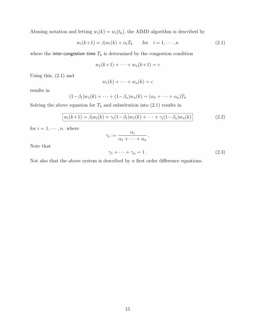
Abusing notation and letting wi(k) = wi(tk), the AIMD algorithm is described by

wi(k+1) = βiwi(k) + αiTk for i = 1, · · · , n (2.1)

where the inter-congestion time Tk is determined by the congestion condition

w1(k+1) + · · ·+ wn(k+1) = c

Using this, (2.1) andw1(k) + · · ·+ wn(k) = c

results in(1−β1)w1(k) + · · ·+ (1−βn)wn(k) = (α1 + · · ·+ αn)Tk

Solving the above equation for Tk and substitution into (2.1) results in

wi(k+1) = βiwi(k) + γi(1−β1)w1(k) + · · ·+ γi(1−βn)wn(k) (2.2)

for i = 1, · · · , n. where

γi :=αi

α1 + · · ·+ αn

.

Note thatγ1 + · · ·+ γn = 1 . (2.3)

Not also that the above system is described by n first order difference equations.

15

2.4 General representation

2.4.1 Continuous-time

With the exception of the discrete-time examples, all of the preceding systems can be de-scribed by a bunch of first order ordinary differential equations of the form

x1 = F1(x1, x2, . . . , xn, u1, u2, . . . , um)x2 = F2(x1, x2, . . . , xn, u1, u2, . . . , um)

...xn = Fn(x1, x2, . . . , xn, u1, u2, . . . , um)

Such a description of a dynamical system is called a state space description; the real scalarvariables, xi(t) are called the state variables; the real scalar variables, ui(t) are called theinput variables and the real scalar variable t is called the time variable. If the system hasoutputs, they are described by

y1 = H1(x1, . . . , xn, u1, . . . , um)y2 = H2(x1, . . . , xn, u1, . . . , um)

...yp = Hp(x1, . . . , xn, u1, . . . , um)

where the real scalar variables, yi(t) are called the output variablesWhen a system has no inputs or the inputs are fixed at some constant values, the system

is described by

x1 = f1(x1, x2, . . . , xn)x2 = f2(x1, x2, . . . , xn)

...xn = fn(x1, x2, . . . , xn)

Limitations of the above description. The above description cannot handle

Systems with delays.Systems described by partial differential equations.

16

Higher order ODE descriptions

Single equation. (Recall the spring-mass-damper system.) Consider a dynamical systemdescribed by a single nth- order differential equation of the form

F (q, q, . . . , q(n), u) = 0

where q(t) is a real scalar and q(n) := dnqdtn

. To obtain an equivalent state space description,we proceed as follows.

(a) First solve for the highest order derivative q(n) of q as a function of q, q, . . . , q(n−1) and uto obtain something like:

q(n) = a(q, q, . . . , q(n−1), u)

(b) Now introduce state variables,

x1 := q

x2 := q...

xn := q(n−1)

to obtain the following state space description:

x1 = x2

x2 = x3

...

xn−1 = xn

xn = a(x1, x2, . . . , xn, u)

17

Multiple equations. (Recall the simple structure and the pendulum cart system.) Con-sider a dynamical system described by N scalar differential equations in N scalar variables:

F1(q1, q1, . . . , q(n1)1 , q2, q2, . . . , q

(n2)2 , . . . , qN , qN , . . . , q

(nN )N , u1, u2, . . . , um ) = 0

F2(q1, q1, . . . , q(n1)1 , q2, q2, . . . , q

(n2)2 , . . . , qN , qN , . . . , q

(nN )N , u1, u2, . . . , um ) = 0

...

FN(q1, q1, . . . , q(n1)1 , q2, q2, . . . , q

(n2)2 , . . . , qN , qN , . . . , q

(nN )N , u1, u2, . . . , um ) = 0

where t, q1(t), q2(t), . . . , qN(t) are real scalars. Note that q(ni)i is the highest order derivative

of qi which appears in the above equations. To obtain an equivalent state space description,we proceed as follows.

(a) Solve for the highest order derivatives, q(n1)1 , q

(n2)2 , . . . , q

(nN )N of q1, · · · , qN which appear

in the differential equations to obtain something like:

q(n1)1 = a1( q1, q1, . . . q

(n1−1)1 , q2, q2, . . . , q

(n2−1)2 , . . . , qN , qN , . . . , q

(nN−1)N , u1, u2, . . . , um )

q(n2)2 = a2( q1, q1, . . . q

(n1−1)1 , q2, q2, . . . , q

(n2−1)2 , . . . , qN , qN , . . . , q

(nN−1)N , u1, u2, . . . , um )

...

q(nN )N = aN( q1, q1, . . . q

(n1−1)1 , q2, q2, . . . , q

(n2−1)2 , . . . , qN , qN , . . . , q

(nN−1)N , u1, u2, . . . , um )

If one cannot uniquely solve for the above derivatives, then one cannot obtain a unique statespace description

(b) As state variables, consider each qi variable and its derivatives up to but not includingits highest order derivative. One way to do this is as follows. Let

x1 := q1 x2 := q1 . . . xn1 := q(n1−1)1

xn1+1 := q2, xn1+2 := q2 . . . xn1+n2 := q(n2−1)2

...

xn1+...+nN−1+1 := qN xn1+...+nN−1+2 := qN . . . xn := q(nN−1)N

where

n := n1 + n2 + . . . + nN

18

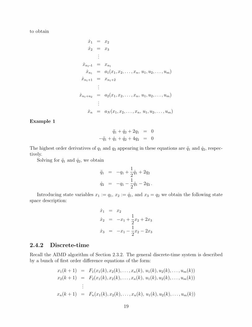
to obtain

x1 = x2

x2 = x3

...

xn1−1 = xn1

xn1 = a1(x1, x2, . . . , xn, u1, u2, . . . , um)

xn1+1 = xn1+2

...

xn1+n2 = a2(x1, x2, . . . , xn, u1, u2, . . . , um)...

xn = aN(x1, x2, . . . , xn, u1, u2, . . . , um)

Example 1

q1 + q2 + 2q1 = 0

−q1 + q1 + q2 + 4q2 = 0

The highest order derivatives of q1 and q2 appearing in these equations are q1 and q2, respec-tively.

Solving for q1 and q2, we obtain

q1 = −q1 +1

2q1 + 2q2

q2 = −q1 − 1

2q1 − 2q2 .

Introducing state variables x1 := q1, x2 := q1, and x3 = q2 we obtain the following statespace description:

x1 = x2

x2 = −x1 +1

2x2 + 2x3

x3 = −x1 − 1

2x2 − 2x3

2.4.2 Discrete-time

Recall the AIMD algorithm of Section 2.3.2. The general discrete-time system is describedby a bunch of first order difference equations of the form:

x1(k + 1) = F1(x1(k), x2(k), . . . , xn(k), u1(k), u2(k), . . . , um(k))

x2(k + 1) = F2(x1(k), x2(k), . . . , xn(k), u1(k), u2(k), . . . , um(k))...

xn(k + 1) = Fn(x1(k), x2(k), . . . , xn(k), u1(k), u2(k), . . . , um(k))

19

The real scalar variables, xi(k), i = 1, 2, . . . , n are called the state variables; the real scalarvariables, ui(k), i = 1, 2, . . . , m are called the input variables and the integer variable k iscalled the time variable. If the system has outputs, they are described by

y1 = H1(x1, . . . , xn, u1, . . . , um)y2 = H2(x1, . . . , xn, u1, . . . , um)

...yp = Hp(x1, . . . , xn, u1, . . . , um)

where the real scalar variables, yi(k), i = 1, 2, . . . , p are called the output variablesWhen a system has no inputs or the inputs are fixed at some constant values, the system

is described by

x1(k + 1) = f1(x1(k), x2(k), . . . , xn(k))x2(k + 1) = f2(x1(k), x2(k), . . . , xn(k))

...xn(k + 1) = fn(x1(k), x2(k), . . . , xn(k))

Higher order difference equation descriptions

One converts higher order difference equation descriptions into state space descriptions in asimilar manner to that of converting higher order ODE descriptions into state space descrip-tions; see Example 2.3.1.

20

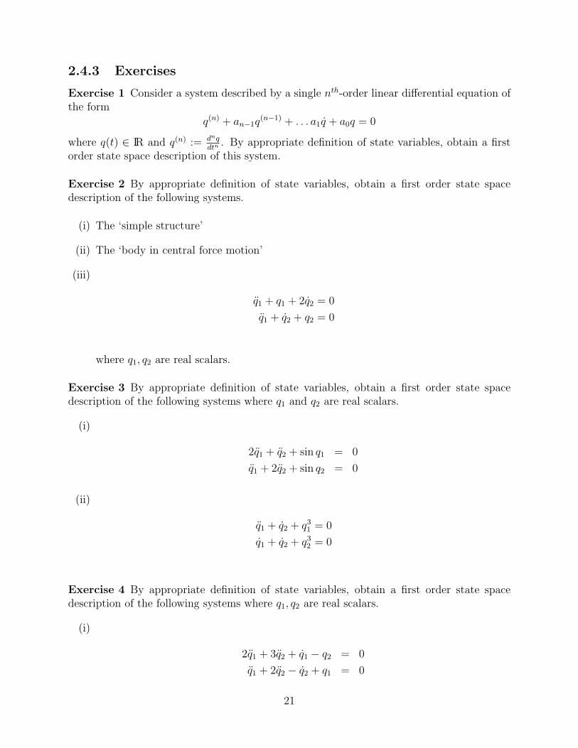
2.4.3 Exercises

Exercise 1 Consider a system described by a single nth-order linear differential equation ofthe form

q(n) + an−1q(n−1) + . . . a1q + a0q = 0

where q(t) ∈ IR and q(n) := dnqdtn

. By appropriate definition of state variables, obtain a firstorder state space description of this system.

Exercise 2 By appropriate definition of state variables, obtain a first order state spacedescription of the following systems.

(i) The ‘simple structure’

(ii) The ‘body in central force motion’

(iii)

q1 + q1 + 2q2 = 0

q1 + q2 + q2 = 0

where q1, q2 are real scalars.

Exercise 3 By appropriate definition of state variables, obtain a first order state spacedescription of the following systems where q1 and q2 are real scalars.

(i)

2q1 + q2 + sin q1 = 0

q1 + 2q2 + sin q2 = 0

(ii)

q1 + q2 + q31 = 0

q1 + q2 + q32 = 0

Exercise 4 By appropriate definition of state variables, obtain a first order state spacedescription of the following systems where q1, q2 are real scalars.

(i)

2q1 + 3q2 + q1 − q2 = 0

q1 + 2q2 − q2 + q1 = 0

21

(ii)

...q2 +2q1 + q2 − q1 = 0

q2 + q1 − q2 + q1 = 0

Exercise 5 By appropriate definition of state variables, obtain a first order state spacedescription of the following systems where q1, q2 are real scalars.

(i)

3q1 − q2 + 2q1 + 4q2 = 0

−q1 + 3q2 + 2q1 − 4q2 = 0

(ii)

3q1 − q2 + 4q2 − 4q1 = 0

−q1 + 3q2 − 4q2 + 4q1 = 0

Exercise 6 Obtain a state-space description of the following single-input single-output sys-tem with input u and output y.

q1 + q2 + q1 = 0

q1 − q2 + q2 = u

y = q1

Exercise 7 Consider the second order difference equation

q(k+2) = q(k+1) + q(k)

Obtain the solution corresponding to

q(0) = 1, q(1) = 1

and k = 0, 1, . . . , 10. Obtain a state space description of this system.

Exercise 8 Obtain a state space representation of the following system:

q(k+n) + an−1q(k+n−1) + . . . + a1q(k+1) + a0q(k) = 0

where q(k) ∈ IR.

22

2.5 Vectors

When dealing with systems containing many variables, the introduction of vectors for systemdescription can considerably simplify system analysis and control design.

2.5.1 Vector spaces and IRn

A scalar is a real or a complex number. The symbols IR and C represent the set of realand complex numbers, respectively. In this section, all the definitions and results are givenfor real scalars. However, they also hold for complex scalars; to get the results for complexscalars, simply replace ‘real’ with ‘complex’ and IR with C.

Consider any positive integer n. A real n-vector x is an ordered n-tuple of real numbers,x1, x2, . . . , xn. This is usually written as x = (x1 , x2 , · · · , xn) or

x =

x1

x2...

xn

or x =

x1

x2...

xn

The real numbers x1, x2, . . . , xn are called the scalar components of x and xi is called thei-th component. The symbol IRn represents the set of ordered n-tuples of real numbers.

Addition

The addition of any two real n-vectors x and y yields another real n-vector x + y which isdefined by:

x + y =

x1

x2...

xn

+

y1

y2...

yn

:=

x1 + y1

x2 + y2...

xn + yn

Zero element of IRn:

0 :=

00...0

Note that we are using the same symbol, 0, for a zero scalar and a zero vector.

The negative of a vector:

−x :=

−x1

−x2...

−xn

23

Properties of addition

(a) (Commutative). For each pair x, y in IRn,

x + y = y + x

(b) (Associative). For each x, y, z in IRn,

(x + y) + z = x + (y + z)

(c) There is an element 0 in IRn such that for every x in IRn,

x + 0 = x

(d) For each x in IRn, there is an element −x in IRn such that

x + (−x) = 0

Scalar multiplication.

The multiplication of an element x of IRn by a real scalar α yields an element of IRn and isdefined by:

αx = α

x1

x2...

xn

:=

αx1

αx2...

αxn

Properties of scalar multiplication

(a) For each scalar α and pair x, y in IRn

α(x + y) = αx + αy

(b) For each pair of scalars α, β and x in IRn,

(α + β)x = αx + βx

(c) For each pair of scalars α, β, and x in IRn,

α(βx) = (αβ)x

(d) For each x in IRn,

1x = x

24

Vector space

Consider any set V equipped with an addition operation and a scalar multiplication oper-ation. Suppose the addition operation assigns to each pair of elements x, y in V a uniqueelement x + y in V and it satisfies the above four properties of addition (with IRn replacedby V). Suppose the scalar multiplication operation assigns to each scalar α and element x inV a unique element αx in V and it satisfies the above four properties of scalar multiplication(with IRn replaced by V). Then this set (along with its addition and scalar multiplication)is called a vector space. Thus IRn equipped with its definitions of addition and scalar mul-tiplication is a specific example of a vector space. We shall meet other examples of vectorsspaces later. An element x of a vector space is called a vector. A vector space with real(complex) scalars is called a real (complex) vector space.

As a more abstract example of a vector space, let V be the set of continuous real-valuedfunctions which are defined on the interval [0,∞); thus, an element x of V is a functionwhich maps [0,∞) into IR, that is, x : [0,∞) −→ IR. Addition and scalar multiplication aredefined as follows. Suppose x and y are any two elements of V and α is any scalar, then

(x + y)(t) = x(t) + y(t)

(αx)(t) = αx(t)

Subtraction in a vector space is defined by:

x− y := x + (−y)

Hence in IRn,

x− y =

x1

x2...

xn

−

y1

y2...

yn

=

x1 − y1

x2 − y2...

xn − yn

2.5.2 IR2 and pictures

An element of IR2 can be represented in a plane by a point or a directed line segment.

25

2.5.3 Derivatives

Suppose x(·) is a function of a real variable t where x(t) is an n-vector. Then

x :=dx

dt:=

dx1

dt

dx2

dt

...

dxn

dt

=

x1

x2

...

xn

2.5.4 MATLAB

Representation of real and complex vectorsAddition and substraction of vectorsMultiplication of a vector by a scalar

26

2.6 Vector representation of dynamical systems

Recall the general descriptions (continuous and discrete) of dynamical systems given inSection 2.4. We define the state (vector) x as the vector with components, x1, x2, · · · , xn,that is,

x :=

x1

x2...

xn

.

If the system has inputs, we define the input (vector) u as the vector with components,u1, u2, · · · , um, that is,

u :=

u1

u2...

um

.

If the system has outputs, we define the output (vector) y as the vector with components,y1, y2, · · · , yp, that is,

y :=

y1

y2...yp

.

We introduce the vector valued functions F and H defined by

F (x, u) :=

F1(x1, x2, . . . , xn, u1, u2, · · · , um)F2(x1, x2, . . . , xn, u1, u2, · · · , um)

...Fn(x1, x2, . . . , xn, u1, u2, · · · , um)

and

H(x, u) :=

H1(x1, x2, . . . , xn, u1, u2, · · · , um)H2(x1, x2, . . . , xn, u1, u2, · · · , um)

...Hp(x1, x2, . . . , xn, u1, u2, · · · , um)

respectively.

Continuous-time systems. The general representation of a continuous-time dynamicalsystem can be compactly described by the following equations:

x = F (x, u)y = H(x, u)

(2.4)

27

where x(t) is an n-vector, u(t) is an m-vector, y(t) is a p-vector and the real variable t isthe time variable. The first equation above is a first order vector differential equation and iscalled the state equation. The second equation is called the output equation.

When a system has no inputs of the input vector vector is constant, it can be describedby

x = f(x) .

A system described by the above equations is called autonomous or time-invariant becausethe right-hand sides of the equations do not depend explicitly on time t. For the first partof the course, we will only concern ourselves with these systems.

However, one can have a system containing time-varying parameters. In this case thesystem might be described by

x = F (t, x, u)

y = H(t, x, u)

that is, the right-hand sides of the differential equation and/or the output equation dependexplicitly on time. Such a system is called non-autonomous or time-varying. We will look atthem later.

Other systems described by higher order differential equations Consider a systemdescribed by

ANy(N) + AN−1y(N−1) + · · ·+ A0y = BMu(M) + BM−1u

(M−1) + · · ·+ B0u

where y(t) is a p-vector, u(t) is an m-vector, N ≥ M , and the matrix AN is invertible. WhenM = 0, we can obtain a state space description with

x =

y...

y(N−1)

When M ≥ 1, we will see later how to put such a system into the standard state space form(2.4).

Discrete-time systems. The general representation of a continuous-time dynamical sys-tem can be compactly described by the following equations:

x(k + 1) = F (x(k), u(k))y(k) = H(x(k), u(k))

(2.5)

where x(k) is an n-vector, u(k) is an m-vector, y(k) is a p-vector and the integer variable kis the time variable. The first equation above is a first order vector difference equation andis called the state equation. The second equation is called the output equation. A systemdescribed by the above equations is called autonomous or time-invariant because the right-hand sides of the equations do not depend explicitly on time k.

28

However, one can have a system containing time-varying parameters. In this case thesystem might be described by

x(k + 1) = F (k, x(k), u(k))

y(k) = H(k, x(k), u(k))

that is, the right-hand sides of the differential equation and/or the output equation dependexplicitly on time. Such a system is called non-autonomous or time-varying.

29

2.7 Solutions and equilibrium states : continuous-time

2.7.1 Equilibrium states

Consider a system described byx = f(x) (2.6)

A solution or motion of this system is any continuous function x(·) satisfying x(t) = f(x(t))for all t.

An equilibrium solution is the simplest type of solution; it is constant for all time, that is,it satisfies

x(t) ≡ xe

for some fixed state vector xe. The state xe is called an equilibrium state. Since an equilibriumsolution must satisfy the above differential equation, all equilibrium states must satisfy theequilibrium condition:

f(xe) = 0

or, in scalar terms,f1(x

e1, x

e2, . . . , x

en) = 0

f2(xe1, x

e2, . . . , x

en) = 0

...fn(xe

1, xe2, . . . , x

en) = 0

Conversely, if a state xe satisfies the above equilibrium condition, then there is a solutionsatisfying x(t) ≡ xe; hence xe is an equilibrium state.

Example 2 Spring mass damper. With u = 0 this system is described by

x1 = x2

x2 = −(k/m)x1 − (c/m)x2 − g .

Hence equilibrium states are given by:

xe2 = 0

−(k/m)xe1 − (c/m)xe

2 − g = 0

Hencexe = 0 =

( −mg/k//0)

This system has a single equilibrium state.

Example 3 The unattached mass. With u = 0 this system is described by

x1 = x2

x2 = 0 .

Hence

xe =

(xe

1

0

)

where xe1 is arbitrary. This system has an infinite number of equilibrium states.

30

Example 4 Pendulum. With u = 0, this system is described by

x1 = x2

x2 = −a sin x1 .

The equilibrium condition yields:

xe2 = 0 and sin(xe

1) = 0 .

Hence, all equilibrium states are of the form

xe =

(mπ0

)

where m is an arbitrary integer. Physically, there are only two distinct equilibrium states

xe =

(00

)and xe =

(π0

)

Higher order ODEs

F (q, q, . . . , q(n)) = 0

An equilibrium solution is the simplest type of solution; it is constant for all time, that is, itsatisfies

q(t) ≡ qe

for some fixed scalar qe. Clearly, qe must satisfy

F (qe, 0, . . . , 0) = 0 (2.7)

For the state space description of this system introduced earlier, all equilibrium statesare given by

xe =

qe

0...0

where qe solves (2.7).

Multiple higher order ODEsEquilibrium solutions

qi(t) ≡ qei , i = 1, 2, . . . , N

HenceF1(q

e1, 0, . . . , qe

2, 0, . . . , . . . , qeN , . . . , 0 ) = 0

F2(qe1, 0, . . . , qe

2, 0, . . . , . . . , qeN , . . . , 0 ) = 0

...FN(qe

1, 0, . . . , qe2, 0, . . . , . . . , qe

N , . . . , 0 ) = 0

(2.8)

31

For the state space description of this system introduced earlier, all equilibrium statesare given by

xe =

qe1

0...qe2

0......

qeN...0

where qe1, q

e2, . . . , q

eN solve (2.8).

Example 5 Central force motion in inverse square gravitational field

r − rω2 + µ/r2 = 0rω + 2rω = 0

Equilibrium solutions

r(t) ≡ re , ω(t) ≡ ωe

Hence,

r, r, ω = 0

This yields−re(ωe)2 + µ/(re)2 = 0

0 = 0

Thus there are infinite number of equilibrium solutions given by:

ωe = ±√

µ/(re)3

where re is arbitrary. Note that, for this state space description, an equilibrium state corre-sponds to a circular orbit.

2.7.2 Exercises

Exercise 9 Find all equilibrium states of the following systems

(i) The first nonlinear system.

(ii) The attitude dynamics system.

(iii) The two link manipulator.

32

2.7.3 Controlled equilibrium states

Consider now a system with inputs described by

x = F (x, u) (2.9)

Suppose the input is constant and equal to ue, that is, u(t) ≡ ue. Then the resulting systemis described by

x(t) = F (x(t), ue)

The equilibrium states xe of this system are given by F (xe, ue) = 0. This leads to thefollowing definition.

A state xe is a controlled equilibrium state of the system, x = F (x, u), if there is a constantinput ue such that

F (xe, ue) = 0

Example 6 (Controlled pendulum)

x1 = x2

x2 = − sin(x1) + u

Any state of the form

xe =

(xe

1

0

)

is a controlled equilibrium state. The corresponding constant input is ue = sin(xe1).

2.8 Solutions and equilibrium states: discrete-time

2.8.1 Equilibrium states

Consider a discrete-time system described by

x(k + 1) = f(x(k)) . (2.10)

A solution of (2.10) is a sequence(

x(0), x(1), x(2), . . .)

which satisfies (2.5).

Example 7 Simple scalar nonlinear system

x(k + 1) = x(k)2

Sample solutions are:

(0, 0, 0, . . .)(−1, 1, 1, . . .)(2, 4, 16, . . . )

33

Equilibrium solutions and states

x(k) ≡ xe

f(xe) = xe

In scalar terms,

f1(xe1, x

e2, . . . , x

en) = xe

1

f2(xe1, x

e2, . . . , x

en) = xe

2

...

fn(xe1, x

e2, . . . , x

en) = xe

m


x(k + 1) = x(k)2

All equilibrium states are given by:(xe)2 = xe

Solving yieldsxe = 0, 1

Example 9 The discrete unattached mass

xe1 + Txe

2 = xe1

xe2 = xe

2

xe =

(xe

1

0

)

where xe1 is arbitrary.

Example 10 (AIMD algoritm) Recalling (2.2) we see that an equilibrium share vectorw must satisfy

wi = βiwi + γi(1−β1)w1 + · · ·+ γi(1−βn)wn for i = 1, · · · , n . (2.11)

Letting

ηi =(1−βi)w1

γi

above equations simplify to

ηi = γ1η1 + · · ·+ γnηn for i = 1, · · · , n .

Thus every solution must satisfy

ηi = K for i = 1, · · · , n .

34

for some K. Since γ1 + · · ·+ γn = 1, it should be K can be any real number. Hence

wi =γiK

1−βi

for i = 1, · · · , n .

Considering w1 + · · ·+ wn = c, the constant K is uniquely given by

K =c

γ1

1−β1+ · · ·+ γn

1−βn

.

2.8.2 Controlled equilibrium states

Consider now a system with inputs described by

x(k+1) = F (x(k), u(k)) (2.12)

Suppose the input is constant and equal to ue, that is, u(k) ≡ ue. Then the resulting systemis described by

x(k+1) = F (x(k), ue)

The equilibrium states xe of this system are given by xe = F (xe, ue). This leads to thefollowing definition.

A state xe is a controlled equilibrium state of the system, x(k+1) = F (x(k), u(k)), if thereis a constant input ue such that

F (xe, ue) = xe

35

2.9 Numerical simulation

2.9.1 MATLAB

>> help ode23

ODE23 Solve differential equations, low order method.

ODE23 integrates a system of ordinary differential equations using

2nd and 3rd order Runge-Kutta formulas.

[T,Y] = ODE23(’yprime’, T0, Tfinal, Y0) integrates the system of

ordinary differential equations described by the M-file YPRIME.M,

over the interval T0 to Tfinal, with initial conditions Y0.

[T, Y] = ODE23(F, T0, Tfinal, Y0, TOL, 1) uses tolerance TOL

and displays status while the integration proceeds.

INPUT:

F - String containing name of user-supplied problem description.

Call: yprime = fun(t,y) where F = ’fun’.

t - Time (scalar).

y - Solution column-vector.

yprime - Returned derivative column-vector; yprime(i) = dy(i)/dt.

t0 - Initial value of t.

tfinal- Final value of t.

y0 - Initial value column-vector.

tol - The desired accuracy. (Default: tol = 1.e-3).

trace - If nonzero, each step is printed. (Default: trace = 0).

OUTPUT:

T - Returned integration time points (column-vector).

Y - Returned solution, one solution column-vector per tout-value.

The result can be displayed by: plot(tout, yout).

See also ODE45, ODEDEMO.

36

>> help ode45

ODE45 Solve differential equations, higher order method.

ODE45 integrates a system of ordinary differential equations using

4th and 5th order Runge-Kutta formulas.

[T,Y] = ODE45(’yprime’, T0, Tfinal, Y0) integrates the system of

ordinary differential equations described by the M-file YPRIME.M,

over the interval T0 to Tfinal, with initial conditions Y0.

[T, Y] = ODE45(F, T0, Tfinal, Y0, TOL, 1) uses tolerance TOL

and displays status while the integration proceeds.

INPUT:

F - String containing name of user-supplied problem description.

Call: yprime = fun(t,y) where F = ’fun’.

t - Time (scalar).

y - Solution column-vector.

yprime - Returned derivative column-vector; yprime(i) = dy(i)/dt.

t0 - Initial value of t.

tfinal- Final value of t.

y0 - Initial value column-vector.

tol - The desired accuracy. (Default: tol = 1.e-6).

trace - If nonzero, each step is printed. (Default: trace = 0).

OUTPUT:

T - Returned integration time points (column-vector).

Y - Returned solution, one solution column-vector per tout-value.

The result can be displayed by: plot(tout, yout).

See also ODE23, ODEDEMO.

2.9.2 Simulink

Simulink is part of Matlab. In Simulink, one describes a system graphically. If one has aSimulink model of a system there are several useful Matlab operations which can be appliedto the system, for example, one may readily find the equilibrium state of the system.

37

2.10 Exercises

Exercise 10 Obtain a state-space description of the following system....q 1 + q2 + q1 = 0

q1 − q2 + q2 = 0

Exercise 11 Recall the ‘two link manipulator’ example in the notes.

(i) By appropriate definition of state variables, obtain a first order state space descriptionof this system.

(ii) Find all equilibrium states.

(iii) Numerically simulate this system using MATLAB. Use the following data and initialconditions:

m1 l1 lc1 I1 m2 l2 lc2 I2 mpayload

kg m m kg.m2 kg m m kg.m2 kg

10 1 0.5 10/12 5 1 0.5 5/12 0

q1(0) =π

2; q1(0) = 0

q2(0) =π

4; q2(0) = 0

Exercise 12 Recall the two pendulum cart example in the notes.

(a) Obtain all equilibrium configurations corresponding to u = 0.

(b) Consider the following parameter sets

m0 m1 m2 l1 l2 g

P1 2 1 1 1 1 1P2 2 1 1 1 0.99 1P3 2 1 0.5 1 1 1P4 2 1 1 1 0.5 1

and initial conditions,

y θ1 θ2 y θ1 θ2

IC1 0 −10 10 0 0 0IC2 0 10 10 0 0 0IC3 0 −90 90 0 0 0IC4 0 −90.01 90 0 0 0IC5 0 100 100 0 0 0IC6 0 100.01 100 0 0 0IC7 0 179.99 0 0 0 0

38

Simulate the system using the following combinations:

P1 : IC1, IC2, IC3, IC4, IC5, IC6, IC7

P2 : IC1, IC2, IC3, IC5.IC7

P3 : IC1, IC2, IC5, IC7

P4 : IC1, IC2, IC3, IC4, IC5, IC6, IC7

39

Chapter 3

Linear time-invariant (LTI) systems

To discuss linear systems, we need matrices. In this section we briefly review some propertiesof matrices. All the definitions and results of this section are stated for real scalars andmatrices. However, they also hold for complex scalars and matrices; to obtain the results forthe complex case, simply replace ‘real’ with ‘complex’ and IR with C.

3.1 Matrices

An m× n matrix A is an array of scalars consisting of m rows and n columns.

A =

a11 a12 . . . a1n

a21 a22 . . . a2n...

......

am1 am2 . . . amn

︸︷︷︸n columns

m rows

The scalars aij are called the elements of A. If the scalars are real numbers, A is called areal matrix. The set of real m× n matrices is denoted by IRm×n

Recall that we can do the following things with matrices.

Matrix addition: A + B

Multiplication of a matrix by a scalar: αA

Zero matrices: 0

Negative of the matrix A: −A

One can readily show that IRm×n with the usual definitions of addition and scalar mul-tiplication is a vector space.

Matrix multiplication: AB

41

Some properties:

(AB)C = A(BC) (associative)

In general AB 6= BA (non-commutative)

A(B + C) = AB + AC

(B + C)A + BA + CA

A(αB) = αAB

(αA)B = αAB

Identity matrix in IRn×n:

I :=

1 0 . . . 00 1 . . . 0...

.... . .

...0 0 . . . 1

= diag (1, 1, . . . , 1)

AI = IA = A

Inverse of a square (n = m) matrix A: A−1

AA−1 = A−1A = I

Some properties:

(αA)−1 =1

αA−1

(AB)−1 = B−1A−1

Transpose of A: AT

Some properties:

(A + B)T = AT + BT

(αA)T = αAT

(AB)T = BT AT

Determinant of a square matrix A : Associated with any square matrix A is a scalar calledthe determinant of A and is denoted by det A.

42

Some properties:

det(AB) = det(A) det(B)

det(AT ) = det(A)

Note that, in general,

det(A + B) 6= det(A) + det(B)

det(αA) 6= α det(A)

The following fact provides a very useful property of determinants.

Fact: A square matrix is invertible iff its determinant is non-zero.

Exercise 13 Compute the determinant and inverse of the following matrix.

(cos θ sin θ

− sin θ cos θ

)

Exercise 14 Prove that if A is invertible then,

det(A−1) =1

det(A)

MATLAB

Representation of real and complex matricesAddition and multiplication of matricesMultiplication of a matrix by a scalarMatrix powersTranspose of a matrixInverse of a matrix

>> help zeros

ZEROS All zeros.

ZEROS(N) is an N-by-N matrix of zeros.

ZEROS(M,N) or ZEROS([M,N]) is an M-by-N matrix of zeros.

ZEROS(SIZE(A)) is the same size as A and all zeros.

>> help eye

EYE Identity matrix.

EYE(N) is the N-by-N identity matrix.

EYE(M,N) or EYE([M,N]) is an M-by-N matrix with 1’s on

the diagonal and zeros elsewhere.

43

EYE(SIZE(A)) is the same size as A.

>> help det

DET Determinant.

DET(X) is the determinant of the square matrix X.

>> help inv

INV Matrix inverse.

INV(X) is the inverse of the square matrix X.

A warning message is printed if X is badly scaled or

nearly singular.

Exercise 15 Determine which of the following matrices are invertible. Obtain the inversesof those which are. Check your answers using MATLAB.

(a)

(1 10 1

)(b)

(1 11 1

)(c)

(0 10 0

)(d)

(0 11 0

)

Exercise 16 Determine which of the following matrices are invertible. Using MATLAB,check your answers and determine the inverse of those that are invertible.

(a)

1 1 00 0 11 0 0

(b)

1 0 11 0 11 0 1

(c)

0 1 01 0 10 1 0

Powers and polynomials of a matrix

Suppose A is a square matrix. We can define powers of a matrix as follows:

A0 := I

A1 := A

A2 := AA...

Ak+1 := AAk

We can also define polynomials of a matrix as follows. If

p(s) = a0 + a1s + a2s2 + . . . + amsm

where a0, . . . , am are scalars, then,

p(A) := a0I + a1A + a2A2 + . . . + amAm

44

Exercise 17 Compute p(A) for the following polynomial-matrix pairs. Check your answersusing MATLAB.

(a)

p(s) = s3 − 3s2 + 3s− 1 A =

1 1 10 1 10 0 1

(b)

p(s) = s2 − 3s A =

1 1 11 1 11 1 1

(c)

p(s) = s3 + s2 + s + 1 A =

1 1 01 1 10 1 1

(d)

p(s) = s3 − 2s A =

0 1 01 0 10 1 0

45

3.2 Linear time-invariant systems


A continuous-time, linear time-invariant (LTI) input-output system can be described by

x = Ax + Buy = Cx + Du

where the n-vector x(t) is the state vector at time t, the m-vector u(t) is the input vector attime t, and the p-vector y(t) is the output vector at time t. The n×n matrix A is sometimescalled the system matrix. The matrices B, C, and D have dimensions n × m, p × n, andp×m, respectively. In scalar terms, this system is described by:

x1 = a11x1 + . . . + a1nxn + b11u1 + . . . + b1mum

...

xn = an1x1 + . . . + annxn + bn1u1 + . . . + bnmum

and

y1 = c11x1 + . . . + c1nxn + d11u1 + . . . + d1mum

...

yp = cp1x1 + . . . + cpnxn + dp1u1 + . . . + dpmum .

A system with no inputs is described by

x = Ax . (3.1)

Example 11 The unattached mass

A =

(0 10 0

), B =

(0

1/m

), C =

(1 0

), D = 0 .

Example 12 Spring-mass-damper

A =

(0 1

−k/m −c/m

), B =

(0

−1

), C =

( −k −c), D = 0 .

Other systems. It should be mentioned that the results of this section and most of thesenotes only apply to finite-dimensional systems, that is, systems whose state space is finite-dimensional. As an example of a system not included here, consider a system with a timedelay T described by

q(t) = A0q(t) + A1q(t−T ) + Bu(T )

y(t) = Cq(t) + Du(t)

As another example, consider any system described by a partial differtial equation, forexample

∂2q

∂t2+ k2 ∂4q

∂η4= 0 .

46

3.2.2 Discrete-time

A discrete-time linear time-invariant (LTI) input-output system can be described by

x(k+1) = Ax(k) + Bu(k)y(k) = Cx(k) + Du(k)

where the n-vector x(k) is the state vector at time k, the m-vector u(k) is the input vectorat time k, and the p-vector y(k) is the output vector at time k. The n × n matrix A issometimes called the system matrix. The matrices B, C, and D have dimensions n × m,p× n, and p×m, respectively.In scalar terms:

x1(k+1) = a11x1(k) + . . . + a1nxn(k) + b11u1(k) + . . . + b1mum(k)...

xn(k+1) = an1x1(k) + . . . + annxn(k) + bn1u1(k) + . . . + bnmum(k)

and

y1 = c11x1 + . . . + c1nxn + d11u1 + . . . + d1mum

...

yp = cp1x1 + . . . + cpnxn + dp1u1 + . . . + dpmum

A system with no inputs is described by

x(k+1) = Ax(k) . (3.2)

Example 13 The discrete unattached mass

A =

(1 T0 1

), B =

(T 2/2mT/m

), C =

(1 0

), D = 0 .

Example 14 AIMD This is a system with no inputs and

A =

β1 + γ1(1− β1) γ1(1− β2) · · · γ1(1− βn)γ2(1− β1) β2 + γ2(1− β2) · · · γ2(1− βn)

.... . .

...γn(1− β1) γn(1− β2) · · · βn + γn(1− βn)

47

3.3 Linearization about an equilibrium solution

In this section we present systematic procedures for approximating a nonlinear system by alinear system. These procedures rely heavily on derivatives.

3.3.1 Derivative as a matrix

Consider an m-vector-valued function f of an n-vector variable x. Suppose that each of thepartial derivatives, ∂fi

∂xj(x∗) exist and are continuous about some x∗.

The derivative of f (Jacobian of f) at x∗ is the following m× n matrix:

Df(x∗) =∂f

∂x(x∗) :=

∂f1

∂x1(x∗) ∂f1

∂x2(x∗) . . . ∂f1

∂xn(x∗)

∂f2

∂x1(x∗) ∂f2

∂x2(x∗) . . . ∂f2

∂xn(x∗)

......

...

∂fm

∂x1(x∗) ∂fm

∂x2(x∗) . . . ∂fm

∂xn(x∗)

.

So,

Df(x∗)ij =∂fi

∂xj

(x∗) ,

that is, the ij-th element of Df is the partial derivative of fi with respect to xj. SometimesDf is written as ∂f

∂x.

Example 15 If

f(x) =

x1x2

cos(x1)ex2

.

then

Df(x) =

x2 x1

− sin(x1) 00 ex2

.

Some properties:

D(f + g) = Df + DgD(αf) = αDf (α is a constant scalar)

(Constant function:) f(x) ≡ c Df(x) = 0(Linear function:) f(x) = Ax Df(x) = A

All linearization is based on the following fundamental property of the derivative. If x∗

and x are any two vectors and x is ‘close’ to x∗, then

f(x) ≈ f(x∗) +∂f

∂x(x∗)(x− x∗)

48

This says that, near x∗, the function can be approximated by a linear function plus a constantterm.

3.3.2 Linearization of continuous-time systems

Consider a continuous-time system described by

x = F (x, u)

y = H(x, u) (3.3)

and suppose xe is an equilibrium state corresponding to a constant input ue; hence,

F (xe, ue) = 0 .

Let ye be the corresponding constant output, that is,

ye = H(xe, ue) .

Sometimes we call the triple (xe, ue, ye) a trim condition of the system. Introducing theperturbed state δx, the perturbed input δu and the perturbed output δy defined by

δx := x− xe, δu := u− ue, δx := u− ue,

the system can also be described by

δx = F (xe+δx, ue+δu)

δy = H(xe+δx, ue+δu)−H(xe, ue)

49

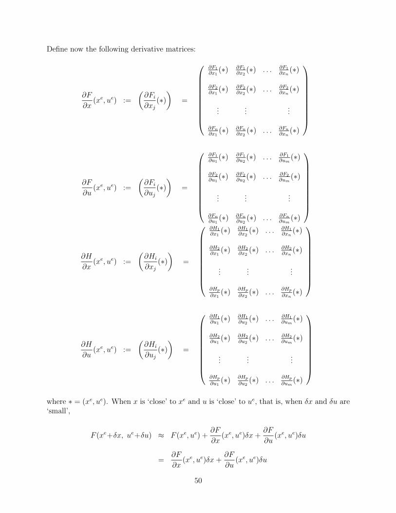
Define now the following derivative matrices:

∂F

∂x(xe, ue) :=

(∂Fi

∂xj

(∗))

=

∂F1

∂x1(∗) ∂F1

∂x2(∗) . . . ∂F1

∂xn(∗)

∂F2

∂x1(∗) ∂F2

∂x2(∗) . . . ∂F2

∂xn(∗)

......

...

∂Fn

∂x1(∗) ∂Fn

∂x2(∗) . . . ∂Fn

∂xn(∗)

∂F

∂u(xe, ue) :=

(∂Fi

∂uj

(∗))

=

∂F1

∂u1(∗) ∂F1

∂u2(∗) . . . ∂F1

∂um(∗)

∂F2

∂u1(∗) ∂F2

∂u2(∗) . . . ∂F2

∂um(∗)

......

...

∂Fn

∂u1(∗) ∂Fn

∂u2(∗) . . . ∂Fn

∂um(∗)

∂H

∂x(xe, ue) :=

(∂Hi

∂xj

(∗))

=

∂H1

∂x1(∗) ∂H1

∂x2(∗) . . . ∂H1

∂xn(∗)

∂H2

∂x1(∗) ∂H2

∂x2(∗) . . . ∂H2

∂xn(∗)

......

...

∂Hp

∂x1(∗) ∂Hp

∂x2(∗) . . . ∂Hp

∂xn(∗)

∂H

∂u(xe, ue) :=

(∂Hi

∂uj

(∗))

=

∂H1

∂u1(∗) ∂H1

∂u2(∗) . . . ∂H1

∂um(∗)

∂H2

∂u1(∗) ∂H2

∂u2(∗) . . . ∂H2

∂um(∗)

......

...

∂Hp

∂u1(∗) ∂Hp

∂u2(∗) . . . ∂Hp

∂um(∗)

where ∗ = (xe, ue). When x is ‘close’ to xe and u is ‘close’ to ue, that is, when δx and δu are‘small’,

F (xe+δx, ue+δu) ≈ F (xe, ue) +∂F

∂x(xe, ue)δx +

∂F

∂u(xe, ue)δu

=∂F

∂x(xe, ue)δx +

∂F

∂u(xe, ue)δu

50

and

H(xe+δx, ue+δu) ≈ H(xe, ue) +∂H

∂x(xe, ue)δx +

∂H

∂u(xe, ue)δu

Hence

δx ≈ ∂F

∂x(xe, ue)δx +

∂F

∂u(xe, ue)δu

δy ≈ ∂H

∂x(xe, ue)δx +

∂H

∂u(xe, ue)δu

This leads to the following definition:

The linearization of system (3.3) about (xe, ue):

δx = A δx + B δuδy = C δx + D δu

(3.4)

where

A =∂F

∂x(xe, ue) , B =

∂F

∂u(xe, ue) , C =

∂H

∂x(xe, ue) , D =

∂H

∂u(xe, ue) .

Example 16 (Simple pendulum.) The linearization of this system about any (xe, ue) isgiven by (3.4) with

A =

(0 1

− cos(xe1) 0

)B =

(01

)C =

(1 0

)D = 0

For eqm. state

xe =

(00

)

we obtain

A =

(0 1−1 0

)

For eqm. state

xe =

(π0

)

we obtain

A =

(0 11 0

)

51

3.3.3 Implicit linearization

This is the way to go when starting from a higher order ODE description.

It is usually easier to first linearize and then obtain a state space description than vice-versa.

For a single equation,F (q, q, . . . , q(n), u) = 0

linearization about an equilibrium solution q(t) ≡ qe corresponding to constant input u(t) ≡ue is defined by:

∂F

∂q(∗)δq +

∂F

∂q(∗)δq + . . . +

∂F

∂q(n)(∗)δq(n) +

∂F

∂u(∗)δu = 0

where (∗) = (qe, 0, 0, . . . , 0), δq = q − qe and δu = u− ue.

For multiple equations, see next example.

Example 17 Orbit mechanics

r − rω2 + µ/r2 = 0

rω + 2rω = 0

Linearization about equilibrium solutions corresponding to constant values re, ωe of r andω, respectively, results in:

δr − (ωe)2δr − (2reωe)δω − (2µ/(re)3)δr = 0

ωeδr + reδω + +2ωeδr + 2reδω = 0

Using the relationship(ωe)2 = µ/(re)3

we obtain

δr − 3(ωe)2δr − (2reωe)δω = 0

reδω + 2ωeδr = 0

Introducing state variables:

x1 := δr, x2 := δr x3 := δω

we obtain a LTI system with system matrix

A =

0 1 03(ωe)2 0 2reωe

0 −2ωe/re 0

52

Example: vehicle lateral dynamics

Consider a vehicle moving in a horizonal plane. We can describe the motion of this vehiclewith the velocity v of its center of gravity (CG) and its yaw rate ψ. The velocity of the masscenter can be described by its magnitude v (the speed of the CG) and the vehicle sideslipangle β which is the angle between v and the vehicle. We will use these three variables todescribe the state of the vehicle. As inputs we consider the steering angle δ of the frontwheels and the braking and acceleration forces Ffx and Frx on the front and rear wheels ofthe vehicle.

Application of Newton’s second law to the vehicle mass center results in

mv = Frx cos β + Fry sin β + Ffx cos(β−δ) + Ffx sin(β−δ) (3.5a)

mv(β + ψ) = −Frx sin β + Fry cos β − Ffx sin(β−δ) + Fry cos(β−δ) (3.5b)

where Ffx, Frx are the longitudinal forces on the front and rear wheels due to braking andacceleration; Ffy, Fry are the lateral forces on the front and rear wheels. Considerations ofangular momentum yield

Jzψ = a(Ffy cos δ + Ffx sin δ)− bFry (3.6)

where Jz is the moment of inertia of the vehicle about the vertical line through its CG, anda, b are the distances between the mass center and the front and rear of the vehicle.

The lateral force Fry depends on the rear sideslip angle αr which is the angle betweenthe rear tires and the velocity of the rear of the vehicle. The lateral force Ffy depends onthe front sideslip angle αf which is the angle between the front tires and the velocity of thefront of the vehicle. Kinematical considerations yield the following relationships:

tan αr = tan β − bψ

v cos β(3.7a)

tan(αf + δ) = tan β +aψ

v cos β(3.7b)

Assuming the lateral forces are zero for zero sideslip angles, and considering Frx = Ffx =δ = 0, the vehicle has an equilibrium with β = ψ = αr = αf = 0 and v an arbitrary constant.

Linearization of the nonlinear equations about these equilibrium conditions results in

δv = a

mv(β + ψ) = −Cαfαf − Cαrαr

Jzψ = −aCαfαf + bCαrαr

αr = β − bψ

v

αf = β +aψ

v− δ

where a = (Frx + Ffx)/m and

Cαf = −dFyf

dαf

and Cαr = −dFyr

dαr

53

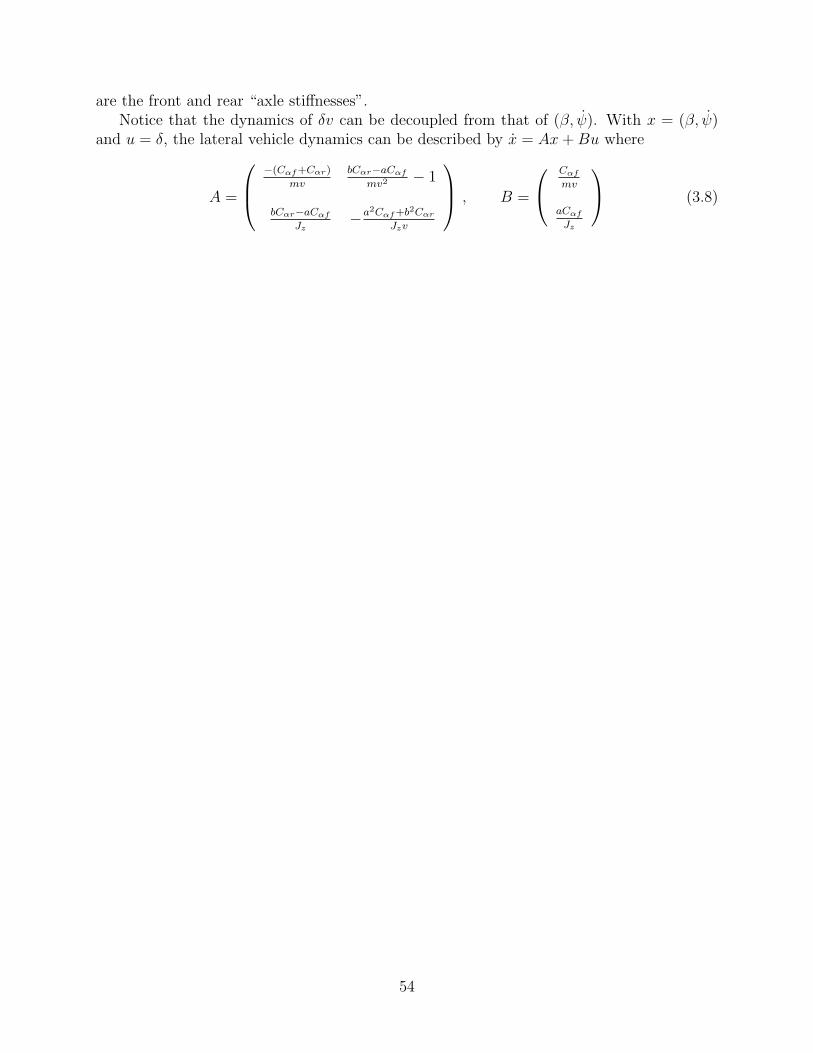
are the front and rear “axle stiffnesses”.Notice that the dynamics of δv can be decoupled from that of (β, ψ). With x = (β, ψ)

and u = δ, the lateral vehicle dynamics can be described by x = Ax + Bu where

A =

−(Cαf+Cαr)

mv

bCαr−aCαf

mv2 − 1

bCαr−aCαf

Jz−a2Cαf+b2Cαr

Jzv

, B =

Cαf

mv

aCαf

Jz

(3.8)

54

3.3.4 Linearization of discrete-time systems

Consider a discrete-time system described by

x(k+1) = F (x(k), u(k))

y(k) = H(x(k), u(k)) (3.9)

and suppose xe, ue, ye is a trim condition, that is,

F (xe, ue) = xe

H(xe, ue) = ye

The linearization of system (3.9) about (xe, ue):

δx(k+1) = Aδx(k) + B δu(k)δy(k) = C δx(k) + D δu(k)

(3.10)

where

A =∂F

∂x(xe, ue) , B =

∂F

∂u(xe, ue) , C =

∂H

∂x(xe, ue) , D =

∂H

∂u(xe, ue) .


x(k+1) = x(k)2

We have xe = 0, 1. For xe = 0:δx(k+1) = 0

For xe = 1:δx(k+1) = 2δx(k)

55

Exercises

Exercise 18 Consider the two-degree-of-freedom spring-mass-damper system described by

mq1 + C(q1 − q2) + K(q1 − q2) + cq1 + kq1 = 0

mq2 + C(q2 − q1) + K(q2 − q1) + cq2 + kq2 = 0

Obtain an A-matrix for a state space description of this system.

Exercise 19 Linearize each of the following systems about the zero equilibrium state.

(i)

x1 = (1 + x21)x2

x2 = −x31

(ii)

x1 = sin x2

x2 = (cos x1)x3

x3 = ex1x2

Exercise 20

(a) Obtain all equilibrium states of the following system:

x1 = 2x2(1− x1)− x1

x2 = 3x1(1− x2)− x2

(b) Linearize the above system about the zero equilibrium state.

Exercise 21 For each of the following systems, linearize about each equilibrium solutionand obtain the system A-matrix for a state space representation of these linearized systems.

(a)q + (q2 − 1)q + q = 0 .

where q(t) is a scalar.

(b)q + q + q − q3 = 0


(c)

(M + m)q + ml θ cos θ −ml θ2 sin θ + kq = 0

mlq cos θ + ml2 θ + mgl sin θ = 0

where q(t) and θ(t) are scalars.

(d)q + 0.5q|q|+ q = 0 .


56

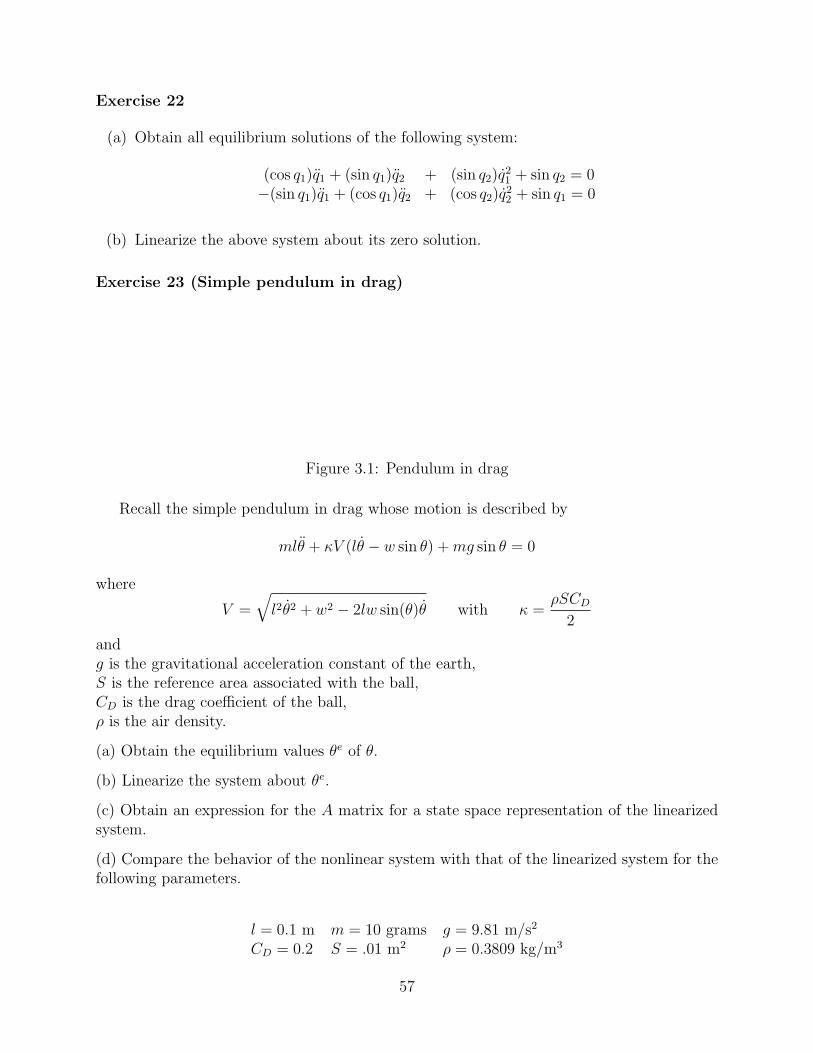
Exercise 22

(a) Obtain all equilibrium solutions of the following system:

(cos q1)q1 + (sin q1)q2 + (sin q2)q21 + sin q2 = 0

−(sin q1)q1 + (cos q1)q2 + (cos q2)q22 + sin q1 = 0

(b) Linearize the above system about its zero solution.

Exercise 23 (Simple pendulum in drag)

Figure 3.1: Pendulum in drag

Recall the simple pendulum in drag whose motion is described by

mlθ + κV (lθ − w sin θ) + mg sin θ = 0

where

V =

√l2θ2 + w2 − 2lw sin(θ)θ with κ =

ρSCD

2

andg is the gravitational acceleration constant of the earth,S is the reference area associated with the ball,CD is the drag coefficient of the ball,ρ is the air density.

(a) Obtain the equilibrium values θe of θ.

(b) Linearize the system about θe.

(c) Obtain an expression for the A matrix for a state space representation of the linearizedsystem.

(d) Compare the behavior of the nonlinear system with that of the linearized system for thefollowing parameters.

l = 0.1 m m = 10 grams g = 9.81 m/s2

CD = 0.2 S = .01 m2 ρ = 0.3809 kg/m3

57

Consider the following cases:

θe w (m/s)0 00 50 150 20

180 20

Illustrate your results with time histories of δθ in degrees. Comment on your results.

58

Chapter 4

Transfer functions

4.1 ←− Transfer functions ←−4.1.1 The Laplace transform

A state space description of an input-output system can be regarded as a time-domaindescription. For linear time-invariant systems, transfer functions provide another way ofdescribing input-output systems; this description is sometimes called a frequency domaindescription.

To discuss transfer functions of continuous-time systems, we need the Laplace transform.Suppose f is a function of time t. Then the Laplace transform of f , which we denote by f orL(f), is a function of a complex variable s and is defined by

f(s) = L(f)(s) =

∫ ∞

0

e−stf(t)dt . (4.1)

Note that f(t) could be a scalar, a vector or a matrix.We will need the following very useful relationship:

L(f)(s) = sf(s)− f(0) (4.2)

The following example illustrates the use of the above relationship.

Example 19 Consider f(t) = eat where a is any scalar. Since f satisfies

f = af

and f(0) = 0, we obtain thatsf(s)− 1 = af(s) .

Hence, as expected, f(s) = 1/(s− a).

59

4.1.2 Transfer functions

Consider now the LTI system

x(t) = Ax(t) + Bu(t)

y(t) = Cx(t) + Du(t)

along with the initial conditionx(0) = x0 .

Taking the Laplace transform of the state equation results in

sx(s)− x0 = Ax(s) + Bu(s)

which can be rewritten as(sI − A)x(s) = x0 + Bu(s)

where x and u are the Laplace transforms of x and u, respectively, Whenever the matrixsI − A is invertible, the above equation may be uniquely solved for x yielding

x(s) = (sI − A)−1x0 + (sI − A)−1Bu(s) .

Taking the Laplace transform of the above output equation yields

y(s) = Cx(s) + Du(s)

where y is the Laplace transform of y. Using the expression for x now results in

y(s) = C(sI − A)−1x0 + G(s)u(s)

where the transfer function (matrix) G(s) is defined by

G(s) = C(sI − A)−1B + D

Zero initial conditions response. Suppose that x(0) = 0. Then, the relationship be-tween the Laplace transform of the input u and the Laplace transform of the output y isgiven by the simple relationship

y = Gu

Sometimes this is represented by

y ←− G ←− u

For a SISO system, we obtain that, for u 6= 0,

G =y

u.

Thus, for a SISO system, the transfer function is the ratio of the Laplace transform ofthe output to the Laplace transform of the input all initial conditions are zero.

60

Example 20

x(t) = −x(t) + u(t)

y(t) = x(t)

Here

G(s) = C(sI − A)−1 + D =1

s + 1

Example 21 Unattached mass

x1 = x2

x2 = u

y = x1

Here

A =

(0 10 0

)B =

(01

)C =

(1 0

)D = 0

Hence

G(s) = C(sI − A)−1B

=1

s2

Exercise 24 Show that the transfer function of

x1 = x2

x2 = −α0x1 − α1x2 + u

y = β0x1 + β1x2

is given by

G(s) =β1s + β0

s2 + α1s + α0

Exercise 25 Show that the transfer function of

x1 = −α0x2 + β0ux2 = x1 −α1x2 + β1uy = x2

is given by

G(s) =β1s + β0

s2 + α1s + α0

61

MATLAB

>> help ss2tf

SS2TF State-space to transfer function conversion.

[NUM,DEN] = SS2TF(A,B,C,D,iu) calculates the transfer function:

NUM(s) -1

H(s) = -------- = C(sI-A) B + D

DEN(s)

of the system:

.

x = Ax + Bu

y = Cx + Du

from the iu’th input. Vector DEN contains the coefficients of the

denominator in descending powers of s. The numerator coefficients

are returned in matrix NUM with as many rows as there are

outputs y.

Example 22 MIMO (Multi-input multi-output) B&B Consider the system illustrated inFigure 4.1 which has two inputs and two outputs. Its motion can be described by

Figure 4.1: B&B

mq1 = k(q2 − q1) + u1

mq2 = −k(q2 − q1) + u2

y1 = q1

y2 = q2

With x1 = q1, x2 = q2, x3 = q1, x4 = q2, we have

A =

0 0 1 00 0 0 1

−k/m k/m 0 0k/m −k/m 0 0

B =

0 00 0

1/m 00 1/m

C =

(1 0 0 00 1 0 0

)D = 0

62

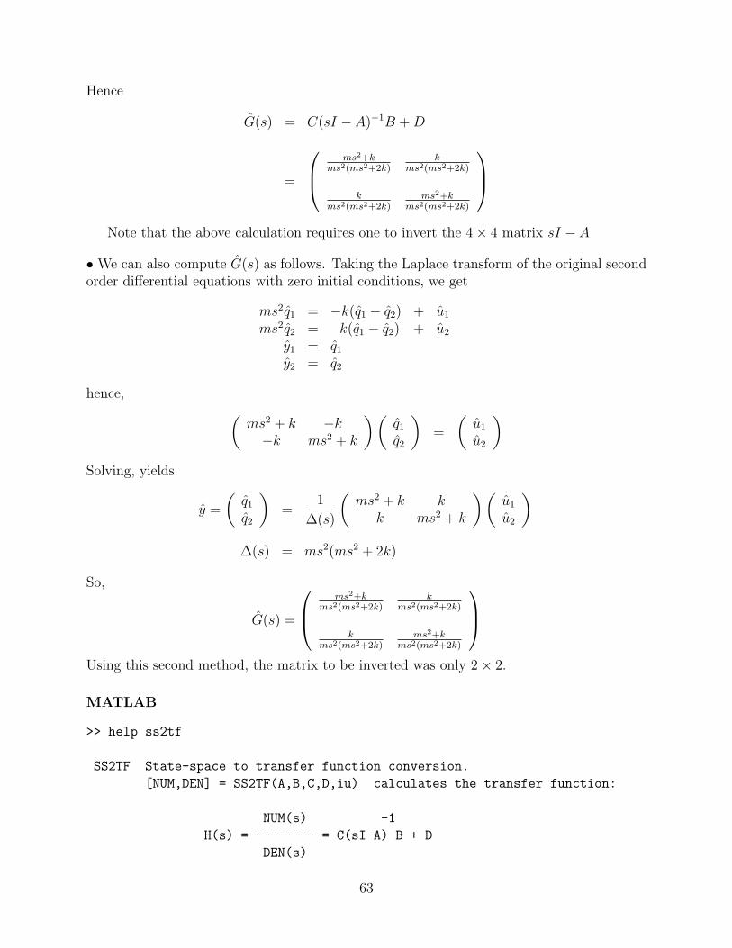
Hence

G(s) = C(sI − A)−1B + D

=

ms2+kms2(ms2+2k)

kms2(ms2+2k)

kms2(ms2+2k)

ms2+kms2(ms2+2k)

Note that the above calculation requires one to invert the 4× 4 matrix sI − A

• We can also compute G(s) as follows. Taking the Laplace transform of the original secondorder differential equations with zero initial conditions, we get

ms2q1 = −k(q1 − q2) + u1

ms2q2 = k(q1 − q2) + u2

y1 = q1

y2 = q2

hence,

(ms2 + k −k−k ms2 + k

)(q1

q2

)=

(u1

u2

)

Solving, yields

y =

(q1

q2

)=

1

∆(s)

(ms2 + k k

k ms2 + k

)(u1

u2

)

∆(s) = ms2(ms2 + 2k)

So,

G(s) =

ms2+kms2(ms2+2k)

kms2(ms2+2k)

kms2(ms2+2k)

ms2+kms2(ms2+2k)

Using this second method, the matrix to be inverted was only 2× 2.

MATLAB

>> help ss2tf

SS2TF State-space to transfer function conversion.

[NUM,DEN] = SS2TF(A,B,C,D,iu) calculates the transfer function:

NUM(s) -1

H(s) = -------- = C(sI-A) B + D

DEN(s)

63

of the system:

.

x = Ax + Bu

y = Cx + Du

from the iu’th input. Vector DEN contains the coefficients of the

denominator in descending powers of s. The numerator coefficients

are returned in matrix NUM with as many rows as there are

outputs y.

See also ltimodels, ss and tf.

Rational transfer functions.

A scalar valued function of a complex variable is rational if it can be expressed as the ratioof two polynomials. It is proper if the order of the numerator polynomial is less than orequal to the order of the denominator polynomial. It is strictly proper if the order of thenumerator polynomial is strictly less than that of the denominator polynomial. A matrixvalued function of a complex variable is rational, proper or strictly proper if each element ofthe matrix function is respectively rational, proper or strictly proper.

Example 23G(s) = s

s2+1rational, strictly proper

G(s) = s2

s2+1rational, proper

G(s) = s3

s2+1rational, not proper

G(s) = e−s

s2+1not rational

We now demonstrate the following result:

The transfer function of a finite-dimensional LTI system is always rational and proper.

The above result follows from the fact that every element Gij of the transfer function ofa finite dimensional LTI system can be expressed as

Gij =Nij

∆(4.3)

where ∆(s) = det(sI−A) is called the characteristic polynomial of A. It is a monic polynomialof order n. A monic polynomial is one whose coefficient of its highest order term is one.Thus

det(sI − A) = sn + αn−1sn−1 + · · ·+ α1s + α0

64

for some scalars α0, · · · , αn−1. The order of the polynomial Nij is at most n. It is less thann if D is zero.

To demonstrate the above fact, recall that the inverse of an invertible n × n matrix Mcan be expressed as

M−1 =1

det(M)adj (M)

where each element of the matrix adj (M) is equal to ± the determinant of an (n−1)× (n−1)submatrix of M . Hence (sI − A)−1 can be expressed as

(sI − A)−1 =1

det(sI − A)adj (sI − A)

where each element of the matrix adj (sI−A) is equal to± the determinant of an (n−1)×(n−1)submatrix of sI −A. Hence, if A is n× n, then each element of adj (sI −A) is a polynomialin s whose degree is at most n− 1. Also, det(sI − A) is a polynomial of order n.

From the above form of (sI − A)−1 it follows that if

G(s) = C(sI − A)−1B

where A is n× n, then

G(s) =1

∆(s)N(s)

where ∆ is the n-th order characteristic polynomial of A , that is, ∆(s) = det(sI − A) andeach element Nij of N is a polynomial of order less than or equal to n−1. So,

Gij =Nij

∆

that is, each element Gij of G is a rational function (ratio of two polynomials) and is strictlyproper (order of numerator strictly less than order of denominator). When each element ofG is rational and strictly proper, we say that G is rational and strictly proper.

IfG(s) = C(sI − A)−1B + D

then

G(s) =1

∆(s)N(s)

where each element Nij of N is a polynomial of order less than or equal to n. So, each

element of G is a rational function and is proper (order of numerator less than or equal toorder of denominator). When each element of G is rational and proper, we say that G isrational and proper.

So, we see that if G is the transfer function of a finite-dimensional LTI system then, Gis rational and proper. Is the converse true? That is, is every proper rational G the transferfunction of some finite-dimensional system and if so, what is(are) the system(s). This isanswered in the next section.

65

Invariance of transfer function under state transformations. The transfer functionof a linear time-invariant system describes the input output behavior of the system when allinitial conditions are zero. Hence, it should be independent of the state variables used in astate space description of the system. We now demonstrate this explicitly.

Suppose G is the transfer function of a system described by

x = Ax + Bu

y = Cx + Du

Then G(s) = C(sI − A)−1B + D. Consider any state transformation

x = Tξ

where T is square and invertible. Then, the system can also be described by

ξ = Aξ + Bu

y = Cξ + Du

withA = T−1AT B = T−1BC = CT D = D

It can be readily verified that

C(sI − A)−1B + D = C(sI − A)−1B + D

that is, the transfer function matrix is unaffected by a state transformation.

Systems described by higher order differential equations. Consider a system de-scribed by

Aly(l) + Al−1y

(l−1) + · · ·+ A0y = Blu(l) + Bl−1u

(l−1) + · · ·+ B0u

where the input u(t) is an m-vector, the output y(t) is a p-vector, l ≥ 1, and the matrix Al

is invertible. How do we put such a system into state space form? By taking the Laplacetransform of the above equation and considering zero initial values for y, y, · · · , y(l−1) andu, u, · · · , u(l−1), we obtain

[slAl + sl−1Al−1 + · · ·+ A0]y(s) = [slBl + sl−1Bl−1 + · · ·+ B0]u(s)

Hence y(s) = G(s)u(s) where

G(s) = [slAl + sl−1Al−1 + · · ·+ A0]−1[slBl + sl−1Bl−1 + · · ·+ B0]

To obtain a state space description of the system under consideration, we could look formatrices A, B, C, D such that G(s) = C(sI − A)−1B + D. We consider this problem in alater section.

66

General input-output systems. Consider any linear input-output system described by

y(t) =

∫ t

0

G(t− τ)u(τ) dτ

where G is Laplace transformable. Then,

y = Gu

where G is the Laplace transform of G.

Example 24

x(t) = −x(t) + u(t− 1)

y(t) = x(t)

Taking Laplace transform with x(0) = 0 yields

sx(s) = −x(s) + e−su(s)

y(s) = x(s)

Hence y(s) = G(s)u(s) with

G(s) =e−s

s + 1

Exercise 26 What is the transfer function of the following system?

x1(t) = x2(t)

x2(t) = u(t− 2)

y(t) = x1(t)

Exercise 27 Obtain the transfer function of the following system

x(t) = −x(t) + 2x(t− h) + u(t)

y(t) = x(t)

4.1.3 Poles and zeros

Poles. Suppose G is a matrix valued function of a complex variable. A complex numberλ is defined to be a pole of G if for some element Gij of G,

lims→λ

Gij(s) = ∞ .

Example 25

67

G(s) poles

1s2+3s+2

-1, -2

s+1s2+3s+2

-2

1s

e−s

s+1

s2

s+1s+1s+2

0, -1, -2

When G(s) = C(sI −A)−1B + D it should be clear that if λ is a pole of G then λ mustbe an eigenvalue of A. However, as the following example illustrates, the converse is notalways true.

Example 26 If,

A =

(0 11 0

)B =

(01

)C =

( −1 1)

D = 0 ,

thendet(sI − A) = s2 − 1

and

G(s) = C(sI − A)−1B =s− 1

s2 − 1=

1

s + 1.

Here A has eigenvalues −1 and 1 whereas G only has a single pole at −1.

We say that a complex number λ is a pole of order m of a transfer function G if λ is apole of G and m is the smallest integer such that λ is not a pole of

(s− λ)mG .

Example 27 The transfer function

G(s) =s + 1

(s− 3)(s + 4)2

has two poles: 3 and −4. The order of the pole at 3 is 1 whereas the order of the pole at −4is 2.

Suppose λ1, λ2, · · · , λl are the poles of a rational transfer function G. Then, it should beclear that we can express G as

G(s) =1

d(s)N(s) (4.4)

whered(s) = (s− λ1)

m1(s− λ2)m2 · · · (s− λl)

ml ,

with mi being the order of the pole λi, and N is a matrix with polynomial elements.

68

Zeroes. Here, we only define zeroes for scalar-input scalar-output transfer functions. Thedefinition of zeroes for MIMO systems is much more complicated. We say that a complexnumber η is a zero of a scalar-input scalar-output transfer function G if

G(η) = 0 . (4.5)

The significance of zeroes. Consider a general LTI SISO system described by

y(t) =

∫ t

0

G(t−τ)u(τ) dτ

Then, the transfer function G of this system is simply the Laplace transform of the impulseresponse G, that is,

G(s) =

∫ ∞

0

e−stG(t) dt .

If we assume that the impulse response G converges to zero exponentially and s is not a poleof G, then it can be shown that the steady-state response of this system to an input

u(t) = est

is given by the output

y(t) = G(s)est

So, we have the following conclusion:

If η is a zero of G then, the steady-state response of the system to the input u(t) = eηt iszero.

Suppose that G is the transfer function of a system with a real impulse response that is,

G(s) =

∫ ∞

0

e−stG(t) dt

where G(t) is real. Using the property that e−st = e−st, the realness of G(t) implies thate−stG(t) = e−stG(t) = e−stG(t); hence

G(s) =

∫ ∞

0

e−stG(t) dt =

∫ ∞

0

e−stG(t) dt =

∫ ∞

0

e−stG(t) dt = G(s) ,

that is,

G(s) = G(s) . (4.6)

Let φ(s) be the argument of the complex number G(s), that is

G(s) = |G(s)|eφ(s) (4.7)

where φ(s) is real. We now show that the steady state response of this system to

u(t) = eαt sin(ωt) ,

69

where α and ω are real numbers, is given by

y(t) = |G(s)|eαt sin(ωt+φ(s)) (4.8)

where s = α + ω. Thus the output has the same form as the input; the non-negative realscalar |G(s)| can be regarded as the system gain at s and φ(s) is the system phase shift at s.

We also obtain the following conclusion:

If η = α + ω is a zero of G then, the steady-state response of the system to the inputu(t) = eαt sin(ωt) is zero.

We also see that the steady state response to a purely sinusoidal input

u(t) = sin(ωt)

is given by

y(t) = |G(ω)| sin(ωt+φ(ω)) (4.9)

To demonstrate the above result, we first note that u(t) = eαt sin(ωt) can be expressedas u(t) = (est − est)/(2) where s = α + ω. So, the corresponding steady state response isgiven by

y(t) = [G(s)est + G(s)est]/2 .

Since G(s) = G(s), we obtain that

y(t) = [G(s)est − G(s)est]/(2) = =(G(s)est

).

Noting thatG(s)est = |G(s)|eφ(s)eαteωt = |G(s)|eαte(ωt+φ(s)) ,

it now follows thaty(t) = |G(s)|eαt sin(ωt + φ(s)) .

Example 28 (Tuned vibration absorber.) Consider a mechanical system subject to asinusoidal disturbance input:

Mq + Cq + Kq = w(t)

where w(t) = A sin(ωt).Attaching a vibration absorber to the system results in

Mq + Cq + Kq − k(η − q) = w (4.10)

mη + k(η − q) = 0 . (4.11)

Taking the Laplace transform of the above equations yields:

(Ms2 + Cs + K + k)q − kη = w (4.12)

(ms2 + k)η − kq = 0 . (4.13)

70

Figure 4.2: Tuned vibration absorber

We see that q = Gw where

G =ms2 + k

∆(s)

and∆(s) = (Ms2 + Cs + K + k)(ms2 + k)− k2 .

This transfer function has zeros at ±√

k/m. if we choose

k/m = ω2

then the steady state response of q to w will be zero.

4.1.4 Discrete-time

The transfer function matrix for

x(k + 1) = Ax(k) + Bu(k)

y(k) = Cx(k) + Du(k)

is defined byG(z) = C(zI − A)−1B + D

where z ∈ C.

4.1.5 Exercises

Exercise 28 (BB in Laundromat.) Consider

mφ1 −mΩ2φ1 + k2(φ1 − φ2) = b1u

mφ2 −mΩ2φ2 − k2(φ1 − φ2) = b2u

y = c1φ1 + c2φ2

For each of the following cases, obtain the system transfer function and its poles; considerω :=

√k/m > Ω.

71

(a)

b1 = 1 b2 = 0

c1 = 1 c2 = 0

(b) (Self excited.)

b1 = 1 b2 = −1

c1 = 1 c2 = 0

(c) (Mass center measurement.)

b1 = 1 b2 = 0

c1 = 1 c2 = 1

(d) (Self excited and mass center measurement.)

b1 = 1 b2 = −1

c1 = 1 c2 = 1

Comment on your results.

72

4.2 Some transfer function properties

4.2.1 Power series expansion and Markov parameters

Suppose G is a transfer function for (A,B, C, D), that is G(s) = C(sI − A)−1B + D. Thenwe will show that, for sufficiently large s, we have the following power series expansion:

G(s) = D +∞∑

k=1

1

skCAk−1B = D +

1

sCB +

1

s2CAB +

1

s3CA2B + · · · .

To see this recall that, for sufficiently large s,

(sI − A)−1 =1

sI +

1

s2A +

1

s3A2 + · · · .

The result follows from this. The coefficient matrices

D, CB, CAB, CA2B, · · ·

are called the Markov parameters of G.

4.2.2 More properties*

Recall that a transfer function G for a finite dimensional system must be rational and proper,that is, it can be expressed as

G =1

dN

where d is a scalar valued polynomial and N is a matrix of polynomials whose degrees arenot greater than that of d. Without loss of generality, we consider d to be monic. Then wecan express d and N as

d(s) = sn + dn−1sn−1 + · · ·+ d1s + d0

N(s) = snNn + sn−1Nn−1 + · · ·+ sN1 + N0

where d0, . . . , dn−1 are scalars and N0, . . . , Nn are constant matrices whose dimensions arethe same as those of G(s). We now show that G = 1

dN is a transfer function for a system

(A,B,C,D) if and only if d satisfies

CAkd(A)B = 0 for k = 0, 1, 2, · · · . (4.14)

and

Nn = D

Nn−1 = CB + dn−1D

Nn−2 = CAB + dn−1CB + dn−2D...

N0 = CAn−1B + dn−1CAn−2B + · · ·+ d1CB + d0D (4.15)

73

To obtain the above result, we first use the power series expansion for G to obtain

1

d(s)N(s) = D +

1

sCB +

1

s2CAB +

1

s3CA2B + · · ·

Multiplying both sides by d(s) yields

snNn + sn−1Nn−1 + · · ·+ sN1 + N0

= [sn + dn−1sn−1 + · · ·+ d1s + d0][D +

1

sCB +

1

s2CAB +

1

s3CA2B + · · · ]

Since the coefficients of like powers of s on both sides of the equation must be equal, thisequation holds if and only if

Nn = D

Nn−1 = CB + dn−1D

Nn−2 = CAB + dn−1CB + dn−2D...

N0 = CAn−1B + dn−1CAn−2B + · · ·+ d1CB + d0D

and

0 = CAnB + dn−1CAn−1B + · · ·+ d0CB

0 = CAn+1B + dn−1CAnB + · · ·+ d0CAB...

0 = CAn+kB + dn−1CAn+k−1B + · · ·+ d0CAkB...

Now note that the first set of equations above is the same as (4.15) while the second set isequivalent to (4.14)

Suppose G is a transfer function for (A,B, C,D) and d is any polynomial for whichd(A) = 0. It follows immediately that (4.15) holds. Hence we can express G as G = 1

dN

where the coefficients of N are computed from (4.14).

A proof of the Cayley Hamilton Theorem. Consider any square matrix A and letG(s) = (sI − A)−1. The function G is the transfer function for the system with B = I,C = I and D = 0. Hence G can be expressed as G = 1

dN where d is the characteristic

polynomial of A. Considering k = 1 in (4.14), it now follows that d(A) = 0.

74

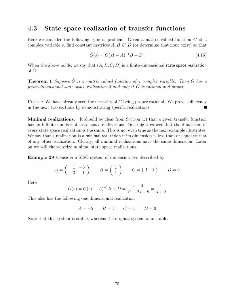
4.3 State space realization of transfer functions

Here we consider the following type of problem: Given a matrix valued function G of acomplex variable s, find constant matrices A,B,C, D (or determine that none exist) so that

G(s) = C(sI − A)−1B + D . (4.16)

When the above holds, we say that (A, B, C, D) is a finite-dimensional state space realizationof G.

Theorem 1 Suppose G is a matrix valued function of a complex variable. Then G has afinite-dimensional state space realization if and only if G is rational and proper.

Proof: We have already seen the necessity of G being proper rational. We prove sufficiencyin the next two sections by demonstrating specific realizations.

Minimal realizations. It should be clear from Section 4.1 that a given transfer functionhas an infinite number of state space realizations. One might expect that the dimension ofevery state space realization is the same. This is not even true as the next example illustrates.We say that a realization is a minimal realization if its dimension is less than or equal to thatof any other realization. Clearly, all minimal realizations have the same dimension. Lateron we will characterize minimal state space realizations.

Example 29 Consider a SISO system of dimension two described by

A =

(1 −3

−3 1

)B =

(11

)C =

(1 0

)D = 0

Here

G(s) = C(sI − A)−1B + D =s− 4

s2 − 2s− 8=

1

s + 2

This also has the following one dimensional realization

A = −2 B = 1 C = 1 D = 0

Note that this system is stable, whereas the original system is unstable.

75

4.4 Realization of SISO transfer functions

4.4.1 Controllable canonical form realization

Suppose that G is a proper rational scalar function of a complex variable s. If G 6= 0, thenfor some positive integer n, the function G can be expressed as

G(s) =βn−1s

n−1 + · · ·+ β1s + β0

sn + αn−1sn−1 + · · ·+ α1s + α0

+ d (4.17)

Note that the denominator polynomial is monic. This is illustrated in the following example.

Example 30 Consider

G(s) =4s + 8

−2s + 10

This is a proper rational function. Also 4s + 8 = −2(−2s + 10) + 28 which results in

G(s) =−2(−2s + 10) + 28

−2s + 10= −2 +

28

−2s + 10=

−14

s− 5− 2 .

When G is expressed in the form shown in (4.17) we now show that

G(s) = C(sI − A)−1B + D

where

G(s) = C(sI − A)−1B + D

where

A =

0 1 0 . . . 0 00 0 1 . . . 0 0...

.... . .

......

.... . .

...0 0 0 . . . 0 1−α0 −α1 −α2 . . . −αn−2 −αn−1

B =

00......01

C =(

β0 β1 β2 . . . βn−2 βn−1

)D = d

(4.18)

It then follows that one can obtain a state space realization of any proper rational scalarSISO transfer function.

To demonstrate the above claim, let ∆ be the denominator polynomial in the aboveexpression for G, that is,

∆(s) := α0 + α1s + . . . + sn

76

and define

v(s) :=

1s...

sn−1

.

Then,

(sI − A)v(s) =

s −1 0 . . . 0 00 s −1 . . . 0 0...

.... . . . . .

......

.... . . . . .

...0 0 0 . . . s −1α0 α1 α2 . . . αn−2 s + αn−1

1s......

ss−2

sn−1

=

00......0

∆(s)

= ∆(s)B

Hence, whenever s is not an eigenvalue of A,

(sI − A)−1B =1

∆(s)v(s)

and

C(sI − A)−1B =1

∆(s)

(β0 β1 . . . βn−1

)

1s...

sn−1

=β0 + β1s + · · ·+ βn−1s

n−1

α0 + α1s + · · ·+ αn−1sn−1 + sn

So,

G(s) = C(sI − A)−1B + D

We will see later why this realization is called controllable.

4.4.2 Observable canonical form realization

Suppose G(s) is a proper rational scalar function of a complex variable s. If G 6= 0, then,for some positive integer n,

G(s) =βn−1s

n−1 + · · ·+ β1s + β0

sn + αn−1sn−1 + · · ·+ α1s + α0

+ d

We will show that

G(s) = C(sI − A)−1B + D

77

where

A =

0 0 . . . 0 −α0

1 0 . . . 0 −α1

0 1. . . 0 −α2

......

. . . . . ....

0 0 . . . 1 −αn−1

B =

β0

β1......

βn−1

C =(

0 0 . . . 0 1)

D = d

• Noting that C(sI − A)−1B + D is a scalar and using the results of the previous section,we have

C(sI − A)−1B + D = BT (sI − AT )−1CT + D = G(s)

We will see later why this realization is called observable.

78

MATLAB

>> help tf2ss

TF2SS Transfer function to state-space conversion.

[A,B,C,D] = TF2SS(NUM,DEN) calculates the state-space

representation:

.

x = Ax + Bu

y = Cx + Du

of the system:

NUM(s)

H(s) = --------

DEN(s)

from a single input. Vector DEN must contain the coefficients of

the denominator in descending powers of s. Matrix NUM must

contain the numerator coefficients with as many rows as there are

outputs y. The A,B,C,D matrices are returned in controller

canonical form. This calculation also works for discrete systems.

To avoid confusion when using this function with discrete systems,

always use a numerator polynomial that has been padded with zeros

to make it the same length as the denominator. See the User’s

guide for more details.

Example 31 Consider

G(s) =s2

s2 + 1

This can be written as

G(s) =−1

s2 + 1+ 1

hence a state space representation is given by

A =

(0 1

−1 0

)B =

(01

)C =

( −1 0)

D = 1

or,

x1 = x2

x2 = −x1 + u

y = −x1 + u

Matlab time:

79

>> num = [1 0 0]

>> den = [1 0 1]

>> [a,b,c,d]=tf2ss(num,den)

a =

0 -1

1 0

b =

1

0

c =

0 -1

d =

1

4.5 Realization of MIMO systems

Suppose G is an p × m proper rational transfer function. Because G is a proper rationalfunction it has a representation of the form

G(s) =1

d(s)N(s) + D (4.19)

where D is a constant p ×m matrix, N is a p ×m matrix of polynomials and d is a scalarvalued monic polynomial.

4.5.1 Controllable realizations

Sometimes it is more convenient to express G as

G(s) = N(s)∆(s)−1 + D (4.20)

where ∆ is a p × m matrix of polynomials. Let us consider this case. Note that if G isexpressed as in (4.19) then, G can be expressed as in (4.20) with ∆(s) = d(s)I where I isthe m×m identity matrix.

Without loss of generality, we can express N and ∆ as

N(s) = sl−1Nl−1 + sl−2Nl−2 + · · ·+ sN1 + N0

∆(s) = slI + sl−1Dl−1 + sl−2Dl−2 + · · ·+ sD1 + D0(4.21)

Here, N0, . . ., Nl−1 are constant p × m matrices while D0, . . ., Dl−1 are constant m × mmatrices. With n = ml, let A, B and C be the following matrices of dimensions n×n, n×m

80

and p× n, respectively,

A =

0 I 0 . . . 0 00 0 I . . . 0 0...

.... . .

......

.... . .

...0 0 0 . . . 0 I

−D0 −D1 −D2 . . . −Dl−2 −Dl−1

, B =

00......0I

, (4.22a)

C =(

N0 N1 N2 . . . Nl−2 Nl−1

). (4.22b)

Note that in the above matrices, I and 0 represent the m ×m identity and zero matrices,respectively. We claim that (A,B, C, D) is a realization of G. This is proven at the end ofthis section.

Note that, when G(s) = 1d(s)

N(s) and d(s) = α0 + α1s + · · ·+ αn−1sn−1 + sn, we have

A =

0 I 0 . . . 0 00 0 I . . . 0 0...

.... . .

......

.... . .

...0 0 0 . . . 0 I

−α0I −α1I −α2I . . . −αl−2I −αl−1I

, B =

00......0I

, (4.23a)

C =(

N0 N1 N2 . . . Nl−2 Nl−1

)(4.23b)

where I and 0 represent the m×m identity and zero matrices, respectively.

Example 32 Consider

G(s) =

3s−2

s+4s2+2s+3

The lowest common denominator (LCD) of the two elements of G(s) is

(s− 2)(s2 + 2s + 3) = s3 − s− 6 =: d(s)

and G(s) = N(s)d(s)−1 where

N(s) =

(3s2 + 6s + 9s2 + 2s− 8

)= s2

(31

)+ s

(62

)+

(9

−8

)

Hence, a controllable realization of G is given by

A =

0 1 00 0 16 1 0

B =

001

C =

(9 6 3

−8 2 1

)D = 0

81

Example 33 Consider the strictly proper rational function,

G(s) =

1s+1

1s2+3s+2

0 1s+2

.

Here G = 1dN where

d(s) = s2 + 3s + 2

and

N(s) =

s + 2 1

0 s + 1

= s

1 0

0 1

+

2 1

0 1

Hence a realization of G is given by

A =

0 0 1 00 0 0 1

−2 0 −3 00 −2 0 −3

B =

0 00 01 00 1

C =

(2 1 1 00 1 0 1

)D =

(0 00 0

)

Here we show that (A,B, C, D) as defined above is a realization of G. Let V be the n×mmatrix of polynomials defined by

V (s) =

IsI...

sl−1I

.

where I represents the m×m identity matrix. Then we have

(sI − A)V (s) =

sI −I 0 . . . 0 00 sI −I . . . 0 0...

.... . . . . .

......

.... . . . . .

...0 0 0 . . . sI −I

D0 D1 D2 . . . Dl−2 sI + Dl−1

IsI......

sl−2Isl−1I

=

00......0

∆(s)

= B∆(s)


(sI − A)−1B = V (s)∆(s)−1

Now note that

CV (s) =(

N0 N1 · · · Nl−1

)

IsI......

sl−2Isl−1I

= N(s) .

82

Hence

C(sI − A)−1B = CV (s)∆(s)−1 = N(s)∆(s)−1

and

G(s) = C(sI − A)−1B + D .

4.5.2 Observable realizations

Sometimes it is more convenient to express G as

G(s) = ∆(s)−1N(s) + D (4.24)

where ∆ is a p × p matrix of polynomials. Note that if G is expressed as in (4.19) then, Gcan be expressed as in (4.24) with ∆(s) = d(s)I where I is the p× p identity matrix.

Without loss of generality, we can express N and ∆ as

N(s) = sl−1Nl−1 + sl−2Nl−2 + · · ·+ sN1 + N0

∆(s) = slI + sl−1Dl−1 + sl−2Dl−2 + · · ·+ sD1 + D0(4.25)

Here, N0, . . ., Nl−1 are constant p × m matrices while D0, . . ., Dl−1 are constant p × pmatrices With n = pl, let A, B and C be the following matrices of dimensions n× n, n×mand p× n, respectively,

A =

−Dl−1 I 0 . . . 0 0−Dl−2 0 I . . . 0 0

......

. . ....

......

. . ....

−D1 0 0 . . . 0 I−D0 0 0 . . . 0 0

, B =

Nn−1

Nn−2......

N1

N0

, (4.26a)

C =(

I 0 0 · · · 0 0)

. (4.26b)

Note that in the above matrices, I and 0 represent the p × p identity and zero matrices,respectively. We claim that (A,B, C, D) is a realization of G. This can be shown as follows.

Let V be the p× n matrix of polynomials defined by

V (s) =(

sl−1I sl−2I · · · sI I)

.

83

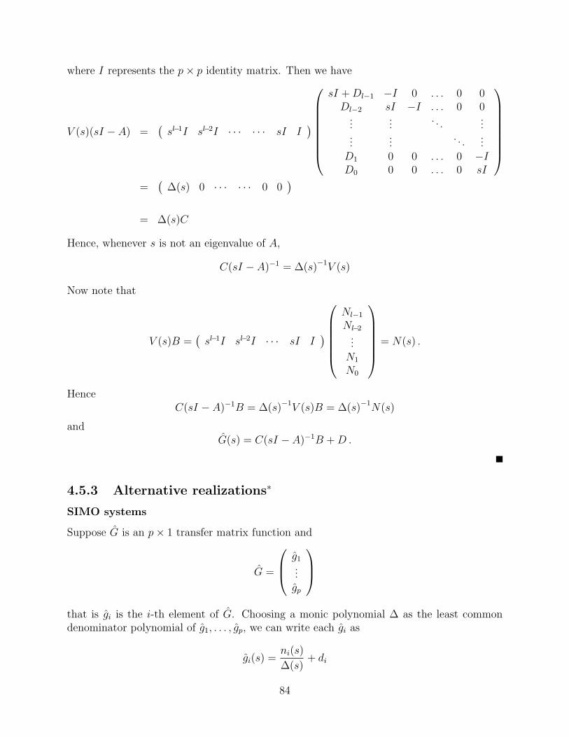
where I represents the p× p identity matrix. Then we have

V (s)(sI − A) =(

sl−1I sl−2I · · · · · · sI I)

sI + Dl−1 −I 0 . . . 0 0Dl−2 sI −I . . . 0 0

......

. . ....

......

. . ....

D1 0 0 . . . 0 −ID0 0 0 . . . 0 sI

=(

∆(s) 0 · · · · · · 0 0)

= ∆(s)C


C(sI − A)−1 = ∆(s)−1V (s)

Now note that

V (s)B =(

sl−1I sl−2I · · · sI I)

Nl−1

Nl−2...

N1

N0

= N(s) .

HenceC(sI − A)−1B = ∆(s)−1V (s)B = ∆(s)−1N(s)

andG(s) = C(sI − A)−1B + D .

4.5.3 Alternative realizations∗

SIMO systems

Suppose G is an p× 1 transfer matrix function and

G =

g1...gp

that is gi is the i-th element of G. Choosing a monic polynomial ∆ as the least commondenominator polynomial of g1, . . . , gp, we can write each gi as

gi(s) =ni(s)

∆(s)+ di

84

where

∆(s) = sn + αn−1sn−1 + · · ·+ α1s + α0

and

ni(s) = βin−1s

n−1 + · · ·+ βi1s + βi

0

Letting

A =

0 1 0 . . . 0 00 0 1 . . . 0 0...

.... . .

......

.... . .

...0 0 0 . . . 0 1−α0 −α1 −α2 . . . −αn−2 −αn−1

B =

00......01

C =

β10 β1

1 β12 . . . β1

n−2 β1n−1

......

......

...βp

0 βp1 βp

2 . . . βpn−2 βp

n−1

D =

d1...dp

we obtain

C(sI − A)−1B + D = G(s)

Example 34 Consider

G(s) =

3s−2

s+4s2+2s+3

The lowest common denominator (LCD) of the two elements of G(s) is

(s− 2)(s2 + 2s + 3) = s3 − s− 6 =: ∆(s)

and G(s) can be expressed as

G(s) =

3s2+6s+9∆(s)

s2+2s−8∆(s)

Hence, a controllable realization of G is given by

A =

0 1 00 0 16 1 0

B =

001

C =

(9 6 3

−8 2 1

)

85

MIMO systems

Suppose G is an p×m transfer matrix function and

G =(

G1 . . . Gm

)

that is Gi is the i-th column of G. Using the results of the previous section, for i = 1, . . . , m,we can obtain matrices Ai, Bi, Ci, Di such that

Gi(s) = Ci(sI − Ai)−1Bi + Di

Let

A =

A1 . . . 0...

. . ....

0 . . . Am

B =

B1 . . . 0...

. . ....

0 . . . Bm

C =(

C1 . . . Cm

)D =

(D1 . . . Dm

)

Then

C(sI − A)−1B + D = G(s)

• Nonminimal realization, in general.

Example 35

G(s) =

1s

1s2

0 1s

The first and second columns of G have realizations

A1 = 0 B1 = 1 C1 =

(10

)D1 = 0

and

A2 =

(0 10 0

)B2 =

(01

)C2 =

(1 00 1

)D2 = 0

respectively. Hence a realization of G is given by

A =

0 0 00 0 10 0 0

B =

1 00 00 1

C =

(1 1 00 0 1

)D =

(0 00 0

)

Note that this transfer function also has the following lower dimensional realization:

A =

(0 10 0

)B =

(1 00 1

)C =

(1 00 1

)D =

(0 00 0

)

86

Exercises

Exercise 29 Obtain a state space realization of the transfer function,

G(s) =s2 + 3s + 2

s2 + 5s + 6.

Is your realization minimal?


G(s) =

11

s− 1

1

s + 1

1

s2 − 1

.

Exercise 31 Obtain a state space realization of the following transfer function.

G(s) =

s+2s+1

1s+3

5s+1

5s+1s+2


G(s) =

1

s− 1

1

s− 1

1

s + 1− 1

s + 1

.


G(s) =

(s

s− 1

1

s + 1

).


Exercise 34 Obtain a state space representation of the following transfer function.

G(s) =

(s2 + 1

s2 − 1

2

s− 1

)

Exercise 35 Obtain a state space representation of the following input-output system.

2d3y

dt3+ 6

d2y

dt2+ 4

dy

dt+ 2y = 6

d2u

dt2+ 10

du

dt+ 8u

Exercise 36 (a) Obtain a state space realization of the following single-input single-outputsystem.

y − 3y − 4y = u− 2u− 8u

87

(b) Is your realization minimal?

Exercise 37 Obtain a state space realization of the following input-output system.

y1 − y1 + y2 = u1 + u1

y2 + y2 − y1 = u2


y1 = u1 + u2

y2 = u1 + u2


y1 + y2 = u2 + u1

y2 + y1 = u1 + u2

Exercise 40 Consider the single-input single-output system described by

x1 = −2x2 + u

x2 = −2x1 + u

y = x1 − x2

(a) Compute eAt for the matrix,

A =

(0 −2

−2 0

).

(b) Obtain the impulse response of the system.

(c) What is the transfer function of this system?

Exercise 41 Consider the single-input single-output system described by

x1 = −3x1 + x2 + w

x2 = x1 − 3x2 + w

y = x1 + x2

(a) Compute eAt for the matrix,

A =

( −3 11 −3

)

(b) Obtain the impulse response of the system.

(c) What is the transfer function of this system?

(d) What are the poles and zeros of the transfer function?

88

Part II

System Behavior and Stability

89

Chapter 5

Behavior of (LTI) systems : I

5.1 Initial stuff


Here we look at the behavior of linear time-invariant systems described by

x = Ax (5.1)

where the state x(t) is a complex n-vector and A is a complex n × n matrix. (The reasonfor complexifying things will be seen shortly.) Sometimes A is called the system matrix.

Solutions. By a solution of system (5.1) we mean any continuous function x(·) which isdefined on some time interval [t0,∞) and which satisfies (5.1). Sometimes we are interestedin solutions which satisfy an initial condition of the form

x(t0) = x0 (5.2)

where t0 is called the initial time and x0 is called the initial state. As a consequence of thelinearity of the system, one can prove the following result:

For each initial condition, system (5.1) has a unique solution.

Shortly, we will study the nature of these solutions.Since the system is time-invariant, knowledge of the solutions for zero initial time, that

is t0 = 0, yields knowledge of the solutions for any other initial time. For suppose x(·) isa solution corresponding to x(0) = x0 . Then, the solution corresponding to x(t0) = x0 isgiven by

x(t) = x(t−t0) .

Since the system is linear, one can readily show that solutions depends linearly on theinitial state; more specifically, there is a matrix valued function Φ (called the state transitionmatrix) such that at each time t the solution due to x(0) = x0 is uniquely given by

x(t) = Φ(t)x0

Later, we develop explicit expressions for Φ.

91

5.1.2 Discrete-time

Here we look at the behavior of linear time-invariant systems described by

x(k+1) = Ax(k)

The state x(k) is a complex n-vector and A is a complex n × n matrix. Sometimes A iscalled the system matrix.

Solutions: Consider initial condition:

x(k0) = x0 (5.3)

Since the system is time-invariant we can, wlog (without loss of generality), consider onlyzero initial time, that is, k0 = 0. For suppose x(·) is a solution corresponding

x(k0) = x0

Thenx(k) = x(k−k0)

where x(·) is the solution corresponding to (5.3).

For k ≥ k0 = 0, we have existence and uniqueness of solutions; specifically,

x(k) = Akx0

Proof: (Example of a proof by induction) Suppose there is a k∗ ≥ 0 for which the aboveholds, that is,

x(k∗) = Ak∗x0

Then

x(k∗+1) = Ax(k∗)

= AAk∗x0

= A(k∗+1)x0

So, if it holds for k∗ it holds for k∗ + 1. Since, x(0) = A0x0, it holds for k∗ = 0. It nowfollows by induction that it holds for all k∗ ≥ 0.

Solution depends linearly on initial state; specifically,

x(k) = Φ(k)x(0) , for k ≥ 0

where Φ(k) = Ak.

92

5.2 Scalar systems


Consider a scalar system described by

x = ax

where x(t) and a are scalars. All solutions are given by:

x(t) = eatx0 ; x0 := x(0)

Real a. So,

(a) If a < 0 you decay with increasing age.

(b) If a > 0 you grow with increasing age.

(c) If a = 0 you stay the same; every state is an equilibrium state.

Figure 5.1: The three types of modes for real scalar systems: α = a

Example 36 (A first example.) Here

a = −c/m < 0

Thus, all solutions are of the form e−(c/m)tx0; hence they decay exponentially.

93

Complex a. Suppose a is a genuine complex number (unreal); that is,

a = α + ω

where α and ω are real numbers. We call α the real part of a and denote this by α = <(a).Similarly, we call ω the imaginary part of a and denote this by ω = =(a).

We now show that the growth behavior of eat depends only on the real part of a. To thisend, we first note that

eat = e(α+ω)t = e(αt+ωt) = eαteωt ,

and, hence, |eat| = |eαt| |eωt|. Since eαt is positive, |eαt| = eαt. Since,

eωt = cos ωt + sin ωt ,

we obtain that |eωt| = 1. Hence,

|eat| = eαt where α = <(a)

Thu, |x(t)| = |eatx0| = |eat||x0| = eαt|x0|. So,

(a) If <(a) < 0 you decay with increasing age.

(b) If <(a) > 0 you grow with increasing age.

(c) If <(a) = 0 your magnitude remains constant.

5.2.2 First order complex and second order real.

Suppose a is a genuine complex number (unreal); that is,

a = α + ω where α = <(a), ω = =(a)

Sincex = ξ1 + ξ2 where ξ1 = <(x), ξ2 = =(x)

Then

ξ1 = αξ1 − ωξ2

ξ2 = ωξ1 + αξ2=

(α −ωω α

)ξ

︸︷︷︸axisymmetric spacecraft

94

Exercise 42 Verify the last set of equations.

Also,

ξ1(t) = eαt cos(ωt)ξ10 − eαt sin(ωt)ξ20

ξ2(t) = eαt sin(ωt)ξ10 + eαt cos(ωt)ξ20=

(eαt cos(ωt) −eαt sin(ωt)eαt sin(ωt) eαt cos(ωt)

)ξ0

where ξ10 = ξ1(0), ξ20 = ξ2(0)

Exercise 43 Verify the last set of equations. Hint: eωt = cos ωt + sin ωt

Figure 5.2: The three complex modes

95

5.2.3 DT

x(k+1) = ax(k)

where x(k) and a are scalars. All solutions are given by:

x(k) = akx0 ; x0 := x(0)

Hence, |x(k)| = |akx0| = |a|k|x0|. So,

(a) If |a| < 1 you decay with increasing age.

(b) If |a| > 1 you grow with increasing age.

(c) If |a| = 1 your magnitude remains the same.

(d) If a = 1 you stay the same; every state is an equilibrium state.

96

5.3 Eigenvalues and eigenvectors

Shortly, we shall see that the behavior of a linear time invariant system is completely deter-mined by the eigenvalues and eigenvectors of its system matrix.

Suppose A is a complex n× n matrix. (The use of the word complex also includes real.To indicate that something is complex but not real we say genuine complex.)

DEFN. A complex number λ is an eigenvalue of A if there is a nonzero vector v such that

Av = λv

The nonzero vector v is called an eigenvector of A corresponding to λ.

So, an eigenvector of A is a nonzero complex n-vector with the property that there is acomplex number λ such that the above relationship holds or, equivalently,

(λI − A)v = 0

Since v is nonzero, λI − A must be singular; so,

det(λI − A) = 0

• The characteristic polynomial of A:

charpoly(A) := det(sI − A)

Note that det(sI − A) is an n-th order monic polynomial, that is, it has the form

det(sI − A) = a0 + a1s + . . . + sn

• We conclude that a complex number λ is an eigenvalue of A if and only if it is a root ofthe nth order characteristic polynomial of A. Hence, A has at least one eigenvalue and atmost n distinct eigenvalues. Suppose A has l distinct eigenvalues, λ1, λ2, . . . , λl; since theseare the distinct roots of the characteristic polynomial of A, we must have

det(sI − A) =l∏

i=1

(s− λi)mi

• The integer mi is called the algebraic multiplicity of λi

• It should be clear that if v1 and v2 are any two eigenvectors corresponding to the sameeigenvalue λ and ξ1 and ξ2 are any two numbers then (provided it is nonzero) ξ1v

1 + ξ2v2

is also an eigenvector for λ. The set of eigenvectors corresponding to λ along with the zerovector is called the eigenspace of A associated with λ. This is simply the null space of λI−A

• The geometric multiplicity of λ is the nullity of λI −A, that is, it is the maximum numberof linearly independent eigenvectors associated with λ.

• It follows that A is invertible if and only if all its eigenvalues are nonzero.

97

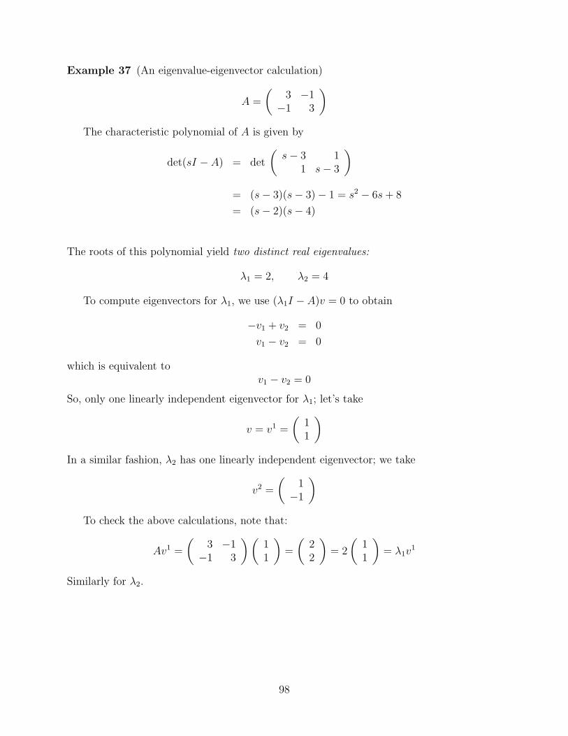
Example 37 (An eigenvalue-eigenvector calculation)

A =

(3 −1

−1 3

)

The characteristic polynomial of A is given by

det(sI − A) = det

(s− 3 1

1 s− 3

)

= (s− 3)(s− 3)− 1 = s2 − 6s + 8

= (s− 2)(s− 4)

The roots of this polynomial yield two distinct real eigenvalues:

λ1 = 2, λ2 = 4

To compute eigenvectors for λ1, we use (λ1I − A)v = 0 to obtain

−v1 + v2 = 0

v1 − v2 = 0

which is equivalent tov1 − v2 = 0

So, only one linearly independent eigenvector for λ1; let’s take

v = v1 =

(11

)

In a similar fashion, λ2 has one linearly independent eigenvector; we take

v2 =

(1

−1

)

To check the above calculations, note that:

Av1 =

(3 −1

−1 3

)(11

)=

(22

)= 2

(11

)= λ1v

1

Similarly for λ2.

98

Example 38 (Another eigenvalue-eigenvector calculation)

A =

(1 1

−1 1

)


det(sI − A) = det

(s− 1 −1

1 s− 1

)= (s− 1)(s− 1) + 1

= s2 − 2s + 2

Computing the roots of this polynomial yields two distinct complex eigenvalues:

λ1 = 1 + , λ2 = 1−

To compute eigenvectors for λ1, we use (λ1I − A)v = 0 to obtain

v1 − v2 = 0

v1 + v2 = 0

which is equivalent to−v1 + v2 = 0

So, only one linearly independent eigenvector; let’s take

v = v1 =

(1

)

(We could also take(

1)T

.) In a similar fashion, λ2 has one linearly independent eigen-vector; we take

v2 =

(1−

)

To check the above calculations, note that

Av1 =

(1 1

−1 1

)(1

)=

(1 +

−1 +

)= (1 + )

(1

)= λ1v

1

Similarly for λ2.

Example 39

A =

(0 10 0

)

Exercise 44 Compute expressions for eigenvalues and linearly independent eigenvectors of

A =

(α ω−ω α

)α, ω 6= 0

99

5.3.1 Real A

Recall Examples 37 and 38. They illustrate the following facts.

• If A is real, its eigenvalues and eigenvectors occur in complex conjugate pairs.

To see this, suppose λ is an eigenvalue of A with eigenvector v. Then

Av = λv

Taking complex conjugate of both sides of this equation yields

Av = λv

Since A is real, A = A; henceAv = λv

that is, λ is an eigenvalue of A with eigenvector v

• Real eigenvectors for real eigenvalues.

• Genuine complex eigenvectors for (genuine) complex eigenvalues.

• The real and imaginary parts of a complex eigenvector are linearly independent.

Example 40 Consider any non-zero angular velocity matrix of the form:

A =

0 −ω3 ω2

ω3 0 −ω1

−ω2 ω1 0

charpoly(A) = s(s2 + Ω2), Ω :=√

ω21 + ω2

2 + ω23

Hence, A has one real eigenvalue 0 and two complex conjugate eigenvalues, Ω,−Ω.

100

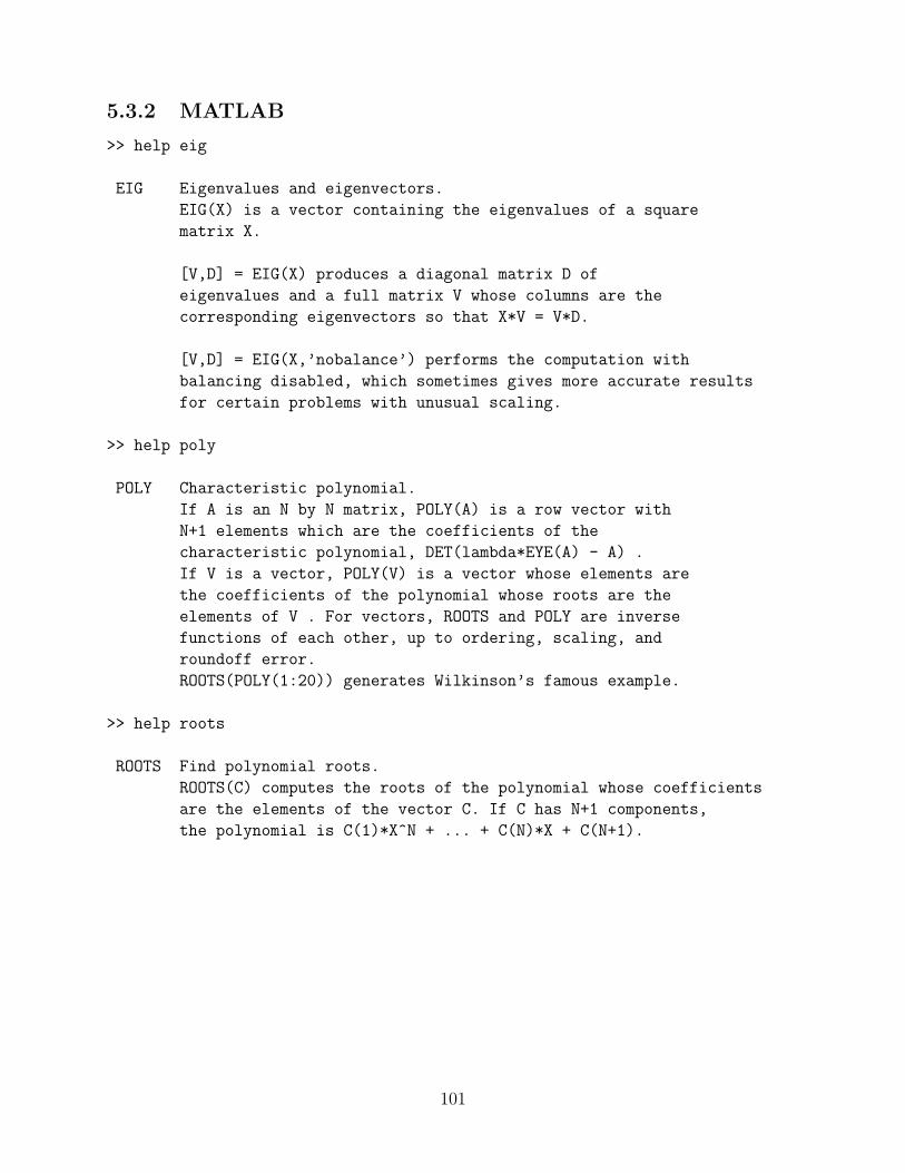
5.3.2 MATLAB

>> help eig

EIG Eigenvalues and eigenvectors.

EIG(X) is a vector containing the eigenvalues of a square

matrix X.

[V,D] = EIG(X) produces a diagonal matrix D of

eigenvalues and a full matrix V whose columns are the

corresponding eigenvectors so that X*V = V*D.

[V,D] = EIG(X,’nobalance’) performs the computation with

balancing disabled, which sometimes gives more accurate results

for certain problems with unusual scaling.

>> help poly

POLY Characteristic polynomial.

If A is an N by N matrix, POLY(A) is a row vector with

N+1 elements which are the coefficients of the

characteristic polynomial, DET(lambda*EYE(A) - A) .

If V is a vector, POLY(V) is a vector whose elements are

the coefficients of the polynomial whose roots are the

elements of V . For vectors, ROOTS and POLY are inverse

functions of each other, up to ordering, scaling, and

roundoff error.

ROOTS(POLY(1:20)) generates Wilkinson’s famous example.

>> help roots

ROOTS Find polynomial roots.

ROOTS(C) computes the roots of the polynomial whose coefficients

are the elements of the vector C. If C has N+1 components,

the polynomial is C(1)*X^N + ... + C(N)*X + C(N+1).

101

5.3.3 Companion matrices

These matrices will be useful later in control design. We met these matrices when construct-ing state space descriptions for systems described by a single higher order linear differentialequation.

Exercise 45 Compute the characteristic polynomial of

(0 1−a0 −a1

)

Hence, write down the characteristic polynomials for the A matrices associated with theunattached mass and the damped linear oscillator.

Exercise 46 Compute the characteristic polynomial of

0 1 00 0 1−a0 −a1 −a2

Fact 1 The characteristic polynomial of

0 1 0 . . . 0 00 0 1 . . . 0 0...

.... . .

......

.... . .

...0 0 0 . . . 0 1−a0 −a1 −a2 . . . −an−2 −an−1

is given byp(s) = a0 + a1s + . . . + an−1s

n−1 + sn

Hence, given any bunch of n complex numbers, there is a companion matrix whose eigen-values are exactly these numbers.

Exercise 47 What is the real 2× 2 companion matrix with eigenvalues 1 + , 1− ?

Exercise 48 What is the companion matrix whose eigenvalues are −1, −2, and −3?

102

5.4 Behavior of continuous-time systems

5.4.1 System significance of eigenvectors and eigenvalues

In this section, we demonstrate that the eigenvalues and eigenvectors of a square matrix Aplay a fundamental role in the behavior of the linear system described by

x = Ax . (5.4)

We first demonstrate the following result.

The system x = Ax has a non-zero solution of the form

x(t) = eλtv (5.5)

if and only if λ is an eigenvector of A and v is a corresponding eigenvector.

To demonstrate the above claim, note that if x(t) = eλtv, then

x = eλtλv and Ax(t) = Aeλtv = eλtAv .

Hence, x(t) = eλtv is a non-zero solution of x = Ax if and only if v is nonzero and

eλtλv = eλtAv .

Since eλt is nonzero, the above condition is equivalent to

Av = λv .

Since v is non-zero, this means λ is an eigenvector of A and v is a corresponding eigenvector.

A solution of the form eλtv is a very special type of solution and is sometimes called amode of the system. Note that if x(t) = eλtv is a solution, then x(0) = v, that is, v is theinitial value of x. Hence, we can make the following statement.

If v is an eigenvector of A, then the solution to x = Ax with initial condition x(0) = vis given by x(t) = eλtv where λ is the eigenvalue corresponding to v.

If v is an eigenvector then, eλtv is also an eigenvector for each t. Also, considering themagnitude of eλtv, we obtain

||eλtv|| = |eλt| ‖v‖ = eαt ‖v‖

where α is the real part of λ. So,

(a) Once an eigenvector, always an eigenvector!

(b) If <(λ) < 0 you decay with increasing age.

(c) If <(λ) > 0 you grow with increasing age.

103

(d) If <(λ) = 0 your magnitude remains constant.

(e) If λ = 0 you stay put; every eigenvector corresponding to λ = 0 is an equilibrium state.

Example 41 The matrix A of example 37 had 2 as an eigenvalue with corresponding eigen-vector [ 1 1 ]T . Hence with initial state,

x0 =

(11

)

the system x = Ax has the following solution:

x(t) =

(e2t

e2t

)

What is the solution for

x0 =

(1

−1

)?

Exercise 49 Prove the following statement. Suppose that v1, . . . , vm are eigenvectors of Awith corresponding eigenvalues, λ1, . . . , λm. Then the solution of (5.4) with initial state

x0 = ξ10v1 + . . . + ξm0v

m ,

where ξ10, . . . , ξm0 are scalars, is given by

x(t) = ξ10eλ1tv1 + . . . + ξm0e

λmtvm .

Behaviour in the v subspace. Suppose v is an eigenvector of A with correspondingeigenvalue λ and consider any initial state of the form x0 = ξ0v. Thus, the initial state x0 isin the 1-dimensional subspace spanned by v. We have shown that the solution correspondingto x(0) = x0 has the form x(t) = ξ(t)v; hence x(t) remains in this subspace. Forgetting aboutthe actual solution, we note that ξv = x = Ax = A(ξv) = λξv. Hence

ξ = λξ ξ(0) = ξ0

In other words, the behavior of the system in the 1-dimensional subspace spanned by v isthat of a scalar system.

Some state space pictures

104

Real systems and complex eigenvalues. Suppose we are interested in the behavior ofa ‘real’ system with real state x and real system matrix A and suppose λ is a (genuine)complex eigenvalue of A, that is,

Av = λv

for a nonzero v. Since A is real and λ is complex, the eigenvector v is complex. The complexsystem can start with a complex initial state but the ‘real’ system cannot. So is the aboveresult useful? It is, just wait.

Since A is real, λ is also an eigenvalue of A with corresponding eigenvector v; hence the(complex) solution corresponding to x(0) = v is given by

eλtv = eλtv

Consider now the real vector

u := <(v) =1

2(v + v)

as an initial state. Since the solution depends linearly on initial state, the solution for thisreal initial state is

1

2(eλtv + eλtv ) = <( eλtv )

Suppose we letα = <(λ) ω = =(λ) w = =(v) .

Thenλ = α + ω and v = u + w .

Hence,

eλtv = eαt(cos ωt + sin ωt)(u + w)

= [eαt cos(ωt) u− eαt sin(ωt) w ] + (eαt sin(ωt) u + eαt cos(ωt) w

)

Hence, the solution due to x(0) = u is

eαt cos(ωt) u− eαt sin(ωt) w

Similarly, the solution due to initial state w is =(eλtv), that is,

eαt sin(ωt) u + eαt cos(ωt) w

• So, if the initial state is of the form

x(0) = ξ10u + ξ20w

where ξ10, ξ20 are any two real scalars (that is, the system starts in the real subspace spannedby the real span of u,w), the resulting solution is given by

x(t) = ξ1(t)u + ξ2(t)w

105

where

ξ1(t) = eαt cos(ωt)ξ10 + eαt sin(ωt)ξ20

ξ2(t) = −eαt sin(ωt)ξ10 + eαt cos(ωt)ξ20=

(eαt cos(ωt) eαt sin(ωt)−eαt sin(ωt) eαt cos(ωt)

)ξ0

Note that, if we let A0 = (ξ210 + ξ2

20)12 and let φ0 be the unique number in the interval [0, 2π)

defined by

sin(φ0) = ξ10/A0 and cos(φ0) = ξ20/A0

then

ξ1(t) = A0eαt sin(ωt+φ0)

ξ2(t) = A0eαt cos(ωt+φ0)

and

x(t) = A0eαt (sin(ωt+φ0)u + cos(ωt+φ0)w)

So, we conclude that for real systems:

(a) If the initial state is in the real 2D subspace spanned by the real and imaginary partsof an complex eigenvector, then so is the resulting solution.

(b) If <(λ) < 0 you decay with increasing age.

(c) If <(λ) > 0 you grow with increasing age.

(d) If <(λ) = 0 your magnitude remains constant and if λ 6= 0 you oscillate forever.

(e) If λ = 0 you stay put; every eigenvector corresponding to λ = 0 is an equilibrium state.

Example 42 Recall example 38. Considering

v = v1 =

(1

)

we have

u =

(10

)w =

(01

)

So,

x = x1u + x2w

Hence, all solutions are given by

x1(t) = eαt cos(ωt)x10 + eαt sin(ωt)x20

x2(t) = −eαt sin(ωt)x10 + eαt cos(ωt)x20=

(eαt cos(ωt) eαt sin(ωt)−eαt sin(ωt) eαt cos(ωt)

)x0

106

Behavior in the u−w subspace. We have shown that if the state starts in the 2-dimensional subspace spanned by u,w, ( let’s call it the u−w subspace) it remains there,that is, if x0 = ξ10u+ ξ20w then x(t) = ξ1(t)u+ ξ2(t)w. Forgetting about the actual solution,we now show that motion in this subspace is described by:

ξ1 = αξ1 + ωξ2

ξ2 = −ωξ1 + αξ2=

(α ω

−ω α

)ξ

To see this, we first equate real and imaginary parts of

A(u + w) = (α + ω)(u + w)

to obtainAu = αu − ωwAw = ωu + αw

Now

ξ1u + ξ2w = x

= Ax

= A(ξ1u + ξ2w)

= ξ1Au + ξ2Aw

= (αξ1 + ωξ2)u + (−ωξ1 + αξ2)w

The desired result now follows by equating coefficients of u and w on both sides of theequation.

Example 43 (Beavis and Butthead) Consider u1 = u2 = 0 in the system in Figure 5.3.

Figure 5.3: Beavis & Butthead

mq1 = k(q2 − q1)mq2 = −k(q2 − q1)

107

Introducing state variables

x1 := q1 , x2 := q2 , x3 := q1 , x4 := q2 ,

this system is described by x = Ax where A is the block partitioned matrix given by

A =

(0 I

A21 0

), A21 = k/m

( −1 11 −1

).


p(s) = s2(s2 + ω2) , ω =√

2k/m

Hence, A has three eigenvalues

λ1 = ω , λ2 = −ω , λ3 = 0 .

Corresponding to each eigenvalue λi, there is at most one linearly independent eigenvectorvi, for example,

v1 =

1−1ω

−ω

, v2 = v1 , v3 =

1100

.

Consider now the subspace S1 spanned by the real and imaginary parts of v1:

S1 = span

1−1

00

,

00ω

−ω

= span

1−1

00

,

001

−1

.

A little reflection reveals that states in this subspace correspond to those states for whichq2 = −q1 and q2 = −q1. A state trajectory which remains in this subspace is characterizedby the condition that

q2(t) ≡ −q1(t) .

We have seen that whenever a motion originates in this subspace it remains there; alsoall motions in this subspace are purely oscillatory and consist of terms of the form cos(ωt)and sin(ωt).

Consider now the subspace S3 spanned by the eigenvector v3. Every state in this subspacehas the form

q1

q1

00

,

that is, q1 is arbitrary, q2 = q1, and q1 = q2 = 0. Since the eigenvalue corresponding to thiseigenspace is zero, every state in this subspace is an equilibrium state.

108

5.4.2 Solutions for nondefective matrices

Recall that the algebraic multiplicity of an eigenvalue of a matrix is the number of timesthat the eigenvalue is repeated as a root of the characteristic polynomial of the matrix. Alsothe geometric multiplicity of an eigenvalue is the dimension of its eigenspace, or equivalently,the maximum number of linearly independent eigenvectors associated with that eigenvalue.It can be proven that the geometric multiplicity of an eigenvalue is always less than or equalto its algebraic multiplicity. An eigenvalue whose geometric multiplicity equals its algebraicmultiplicity is call a nondefective eigenvalue. Otherwise, it is called defective. If an eigenvalueis not repeated, that is, it is not a repeated root of the matrix characteristic polynomial, thenit has algebraic multiplicity one. Since its geometric multiplicity must be greater than zeroand less than or equal to its algebraic multiplicity, it follows that its geometric multiplicityequals its algebraic multiplicity; hence the eigenvalue is nondefective.

A matrix with the property that all its eigenvalues are nondefective is called a nondefectivematrix. Otherwise, it is called defective. When is a matrix A nondefective? Some examplesare:

(a) A has n distinct eigenvalues where A is n× n.

(b) A is hermitian that is, A∗ = A.

(c) A is unitary, that is, A∗A = I.

Here A∗ is the complex conjugate transpose of A.We have the following result.

Fact 2 An n× n matrix has n linearly independent eigenvectors if and only if A is nonde-fective.

Example 44 The following matrix is a simple example of a defective matrix.

A =

(0 10 0

)

Example 45 The following matrix is another example example of a defective matrix.

A =

0 1 0 0−ω2 0 1 0

0 0 0 10 0 −ω2 0

where ω is any real number.

Suppose A is a nondefective matrix and consider any initial condition: x(0) = x0. SinceA is nondefective, it has a basis of eigenvectors v1, · · · , vn. Hence, there are unique scalarsξ10, ξ10, . . . , ξn0 such that x0 can be expressed as

x0 = ξ10v1 + ξ20v

2 + . . . + ξn0vn .

109

From this it follows that the solution due to x(0) = x0 is given by

x(t) = eλ1tξ10v1 + eλ2tξ20v

2 + . . . + eλntξn0vn (5.6)

Note that each term eλitξi0vi on the right-hand-side of the above equation is a mode. This

results in the following fundamental observation.

Every motion (solution) of a linear time-invariant system with nondefective A matrix issimply a sum of modes.

5.4.3 Defective matrices and generalized eigenvectors

Consider a square matrix A. Then we have the following fact.

Fact 3 An eigenvalue λ for A is defective if and only if there is a nonzero vector g such that

(A− λI)2g = 0 but (A− λI)g 6= 0 .

The vector g is called a generalized eigenvector for A.

Example 46

A =

(0 10 0

)

Consider λ = 0. Then

g =

(01

)

is a generalized eigenvector of A.

We now demonstrate the consequence of a system having a defective eigenvalue. So,suppose λ is a defective eigenvalue for a square matrix A. Let g be any correspondinggeneralized eigenvector for λ. We now show that

x(t) = eλtg + teλt(A− λI)g

is a solution of x = Ax. To see this, differentiate x to obtain

x(t) = eλtλg + eλt(A− λI)g + teλtλ(A− λI)g

= eλtAg + teλtλ(A− λI)g

Since (A− λI)2g = 0, we have

A(A− λI)g = λ(A− λI)g .

Hence

x(t) = eλtAg + teλtA(A− λI)g = A(eλtg + teλt(A− λI)g)

= Ax(t) .

110

Consider the function given by teλt and note that

|teλt| = |t|eαt

where α is the real part of λ. So, if α is negative, the magnitude of the above function decaysexponentially. If α is positive, the magnitude of the above function grows exponentially. Ifα is zero, the magnitude of the above function is given by |t| which is also unbounded. Fromthis discussion, we see that the defectiveness of an eigenvalue is only significant when theeigenvalue lies on the imaginary axis of the complex plane, that is when it has zero real part.

Example 47 (Resonance) Consider a simple spring-mass system, of mass m and springconstant k, subject to a sinusoidal force w(t) = A sin(ωt + φ) where ω =

√k/m is the

unforced natural frequency of the spring mass system and A and φ are arbitrary constants.Letting q be the displacement of the mass from its unforced equilibrium position, the motionof this system can be described by

mq + kq = w .

Figure 5.4: Resonance

Since w(t) = A sin(ωt + φ) it satisfies the following differential equation:

w + ω2w = 0 .

If we introduce state variables,

x1 = q , x2 = q , x3 = w , x4 , = w

the sinusoidally forced spring-mass system can be described by x = Ax where

A =

0 1 0 0−ω2 0 1/m 0

0 0 0 10 0 −ω2 0

.

This matrix has characteristic polynomial

p(s) = (s2 + ω2)2 .

111

Hence A has two distinct imaginary eigenvalues λ1 = ω and λ2 = −ω, both of which arerepeated twice as roots of the characteristic polynomial. All eigenvalues for λ1 and λ2 are ofthe form cv1 and cv2, respectively, where

v1 =

1ω00

and v2 =

1−ω

00

.

Since these eigenvalues have algebraic multiplicity two and geometric multiplicity one, theyare defective. A generalized eigenvector corresponding to λ1 and λ2 is given by

g1 =

1/2k01ω

and g2 =

1/2k01−ω

,

respectively. Hence this system has solutions with terms of the form t sin(ωt).

Exercises

Exercise 50 (Beavis and Butthead at the laundromat)

mq1 −mΩ2q1 + k2(q1 − q2 − 2l0) = 0

mq2 −mΩ2q2 − k2(q1 − q2 − 2l0) = 0

with

ω :=√

k/m > Ω

Figure 5.5: At the laundromat

(a) Obtain the equilibrium values qe1, q

e2 of q1, q2.

112

(b) With

x1 = δq1 := q1 − qe1

x2 = δq2 := q2 − qe2

x3 = q1

x4 = q2

Obtain a state space description of the form x = Ax.

(c) Obtain expressions for the eigenvalues of A. Write down expressions for the complexJordan form and the real Jordan form of A?

(d) For the rest of the exercise, consider ω2 = 2Ω2. Obtain expressions for linearly inde-pendent eigenvectors of A.

(e) For the rest of the exercise, let Ω = 1. Numerically simulate with initial conditions

δq1(0) = 1, δq2(0) = −1, q1(0) = 0, q2(0) = 0

On the same graph, plot δq1(t) and −δq2(t) vs t. Why is δq2(t) ≡ −δq1(t)? Plot δq2(t)vs δq1(t).

(f) Numerically simulate with initial conditions

δq1(0) = 1, δq2(0) = 1, q1(0) = −1, q2(0) = −1

On the same graph, plot δq1(t) and δq2(t) vs t. Why is δq2(t) ≡ δq1(t)? Why does thesolution decay to zero? Plot δq2(t) vs δq1(t).

(g) Numerically simulate with initial conditions

δq1(0) = 1, δq2(0) = 1, q1(0) = 1, q2(0) = 1

On the same graph, plot δq1(t) and δq2(t) vs t. Why is δq2(t) ≡ δq1(t)? Is this solutionbounded? Plot δq2(t) vs δq1(t).

(h) Numerically simulate with initial conditions

δq1(0) = 1, δq2(0) = −1, q1(0) = , q2(0) = −

Compute ||x(t)|| and show (by plotting ||x|| vs t) that it is constant. Why is it constant?

Exercise 51 Consider the delay differential equation described by

x(t) = A1x(t) + A2x(t− 1)

where t ∈ IR and x(t) ∈ Cn. Show that if a complex number λ satisfies

det(λI − A1 − e−λA2) = 0

then the delay differential equation has a solution of the form

eλtv

where v ∈ Cn is nonzero.

113

Exercise 52 Consider a system described by

Mq + Cq + Kq = 0

where q(t) is an N -vector and M , C and K are square matrices. Suppose λ is a complexnumber which satisfies

det(λ2M + λC + K) = 0 .

Show that the above system has a solution of the form

q(t) = eλtv

where v is a constant N -vector.

114

5.5 Behavior of discrete-time systems

5.5.1 System significance of eigenvectors and eigenvalues

Consider now a discrete time system described by

x(k+1) = Ax(k) (5.7)


The discrete-time system (5.7) has a solution of the form

x(k) = λkv (5.8)

if and only if λ is an eigenvalue of A and v is a corresponding eigenvector.

To prove this, we first suppose that λ is an eigenvalue of A with v as a correspondingeigenvector. We need to show that x(k) = λkv is a solution of (5.7). Since Av = λv, itfollows that x(k+1) = λ(k+1)v = λkλv = λkAv = A(λkv) = Ax(k), that is x(k+1) = Ax(k);hence x(·) is a solution of (5.7).

Now suppose that x(k) = λkv is a solution of (5.7). Then λv = x(1) = Ax(0) = Av, thatis, Av = λv; hence λ is an eigenvalue of A and v is a corresponding eigenvector.

A solution of the form λkv is a very special type of solution and is sometimes called amode of the system. Note that if x(k) = λkv is a solution, then x(0) = v, that is, v is theinitial value of x. Hence, we can make the following statement.

If v is an eigenvector of A, then the solution to x(k+1) = Ax(k) with initial conditionx(0) = v is given by x(k) = λkv where λ is the eigenvalue corresponding to v.

If v is an eigenvector then, λkv is also an eigenvector for each k. Also, considering themagnitude of λkv, we obtain

||λkv|| = |λk| ‖v‖ = |λ|k ‖v‖

So,

(a) Once an eigenvector, always an eigenvector!

(b) If |λ| < 1 you decay with increasing age.

(c) If |λ| > 1 you grow with increasing age.

(d) If |λ| = 1 and λ 6= 1 you oscillate forever.

• If λ = 1 and x(0) = v, then x(k) = v for all k, that is v is an equilibrium state for thesystem.• If λ = 0 and x(0) = v, then x(k) = 0 for all k > 0, that is the state of the system goes tozero in one step.

115

5.5.2 All solutions for nondefective matrices

Recall that an eigenvalue whose geometric multiplicity equals its algebraic multiplicity iscalled a nondefective eigenvalue. Otherwise, it is considered defective. A matrix with theproperty that all its eigenvalues are nondefective is called a nondefective matrix. Otherwise,it is considered defective. Recall also that an n × n matrix has n linearly independenteigenvectors if and only if A is nondefective.

Example 48 The following matrix is a simple example of a defective matrix.

A =

(0 10 0

)

Suppose A is a nondefective matrix and consider any initial condition: x(0) = x0. SinceA is nondefective, it has a basis of eigenvectors v1, · · · , vn. Hence,

x0 = ξ10v1 + ξ20v

2 + . . . + ξn0vn

From this it follows that

x(k) = λk1ξ10v

1 + λk2ξ20v

2 + . . . + λknξn0v

n (5.9)

Note that each term λki ξi0v

i on the right-hand-side of the above equation is a mode. Thisresults in the following fundamental observation.

Every motion (solution) of a discrete-time linear time-invariant system with nondefectiveA matrix is simply a sum of modes.

5.5.3 Some solutions for defective matrices

Consider a square matrix A and recall that an eigenvalue λ for A is defective if and only ifthere is a nonzero vector g such that

(A− λI)2g = 0 but (A− λI)g 6= 0 .

The vector g is called a generalized eigenvector for A.

Example 49

A =

(0 10 0

)

Consider λ = 0. Then

g =

(01

)

is a generalized eigenvector of A.

116

We now demonstrate the consequence of a system having a defective eigenvalue. So,suppose λ is a defective eigenvalue for a square matrix A. Let g be any correspondinggeneralized eigenvector for λ. We now show that

x(k) = λkg + kλ(k−1)(A− λI)g

is a solution of x(k+1) = Ax(k). To see this, we first note that, since (A − λI)2g = 0, wehave

A(A− λI)g = λ(A− λI)g .

Hence

Ax(k) = λkAg + kλ(k−1)A(A− λI)g

= λkAg + kλk(A− λI)g .

Now note that

x(k+1) = λ(k+1)g + (k+1)λk(A− λI)g

= λ(k+1)g + kλk(A− λI)g + λkAg − λ(k+1)g

= λkAg + kλk(A− λI)g .

Hence x(k+1) = Ax(k)

Consider the function given by kλk−1 and note that

|kλk−1| = |k||λ|k−1 .

So, if |λ| < 1, the magnitude of the above function decays exponentially. If |λ| > 1,the magnitude of the above function grows exponentially. If |λ| = 1, the magnitude of theabove function is given by |k| which is also unbounded. From this discussion, we see that thedefectiveness of an eigenvalue is only significant when the eigenvalue lies on the unit circlein the complex plane, that is when its magnitude is one.

117

5.6 Similarity transformations

Motivating example. Consider

x1 = 3x1 − x2

x2 = −x1 + 3x2

Suppose we define new states:

ξ1 = (x1 + x2)/2

ξ2 = (x1 − x2)/2

Then,

ξ1 = 2ξ1

ξ2 = 4ξ2

That looks better!

Where did new states come from? First note that

x1 = ξ1 + ξ2

x2 = ξ1 − ξ2

and we have the following geometric interpretation. Since,

x = x1

(10

)+ x2

(01

)

= ξ1

(11

)+ ξ2

(1−1

)

the scalars x1, x2 are the coordinates of the vector x wrt the usual basis for IR2; the scalarsξ1, ξ2 are the coordinates of x wrt the basis

(11

) (1

−1

)

Where did these new basis vectors come from? These new basis vectors are eigenvectors ofthe matrix

A =

(3 −1

−1 3

)

and the system is described by x = Ax.

118

Coordinate transformations. Suppose we have n scalar variables x1, x2, . . . , xn and weimplicitly define new scalar variables ξ1, ξ2, . . . , ξn by

x = Tξ where x =

x1

x2...

xn

and ξ =

ξ1

ξ2...ξn

and T is an n× n invertible matrix. Then, ξ is explicitly given by

ξ = T−1x

We can obtain a geometric interpretation of this change of variables as follows. First,observe that

x1

x2...

xn

︸︷︷︸x

= x1

10...0

︸︷︷︸e1

+ x2

01...0

︸︷︷︸e2

+ . . . + xn

00...1

︸︷︷︸en

,

that is the scalars x1, x2, . . . , xn are the coordinates of the vector x wrt the standard basise1, e2, . . . , en, or, x is the coordinate vector of itself wrt the standard basis. Suppose

T =(

t1 . . . tj . . . tn)

that is, tj is the j-th column of T . Since T is invertible, its columns, t1, t2, . . . , tn, form abasis for Cn. Also, x = Tξ can be written as

x = ξ1t1 + ξ2t

2 + . . . + ξntn

From this we see that ξ1, ξ2, . . . , ξn are the coordinates of x wrt to the new basis and thevector ξ is the coordinate vector of the vector x wrt this new basis. So x = Tξ defines acoordinate transformation.

Similarity transformations. Consider now a CT (DT) system described by

x = Ax ( x(k+1) = Ax(k) )

and suppose we define new state variables by x = Tξ where T is nonsingular; then thebehavior of ξ is governed by

ξ = Λξ ( ξ(k+1) = Λξ(k) )

whereΛ = T−1AT

A square matrix A is said to be similar to another square matrix Λ if there exists anonsingular matrix T such that Λ = T−1AT .

Recalling that the columns t1, t2, . . . , tn of T form a basis, we have now the following veryuseful result.

119

Useful result. Suppose

Atj = α1jt1 + α2jt

2 + . . . + αnjtn

Then the matrix Λ = T−1AT is uniquely given by

Λij = αij

that is Λij is the i-th coordinate of the vector Atj wrt the basis t1, t2, · · · , tn. Thus, the j-thcolumn of the matrix Λ is the coordinate vector of Atj wrt the basis t1, t2, · · · , tn.

Proof. Premultiply Λ = T−1AT by T to get:

TΛ = AT

On the right we have

AT = A(

t1 . . . tj . . . tn)

=(

At1 . . . Atj . . . Atn)

And on the left,

TΛ =(

t1 t2 . . . . . . tn)

Λ11 . . . Λ1j . . . Λ1n

Λ21 . . . Λ2j . . . Λ2n...

......

......

...Λn1 . . . Λnj . . . Λnn

=

(Λ11t

1 + · · ·+ Λn1tn ... . . . . . .

... Λ1jt1 + . . . + Λnjt

n

︸︷︷︸j-th column

... . . . . . .... Λ1nt

1 + . . . + Λnntn

)

Comparing the expressions for the j-th columns of AT and TΛ yields

Λ1jt1 + . . . + Λnjt

n = Atj

= α1jt1 + . . . + αnjt

n

Since the bi’s form a basis we must have Λij = αij.

• Note thatA = TΛT−1

Example 50 Recall example 37. Note that the eigenvectors v1 and v2 are linearly indepen-dent; hence the matrix

T :=(v1 v2

)=

(1 11 −1

)

120

is invertible. Since

Av1 = 2v1

Av2 = 4v2

we can use the above result and immediately write down (without computing T−1)

Λ = T−1AT =

(2 00 4

)

Explicitly compute T−1 and then T−1AT to check.

Example 51 Recalling example 38 we can follow the procedure of the last example anddefine

T :=

(1 1 −

)

to obtain (without computing T−1)

Λ = T−1AT =

(1 + 0

0 1−

)

You may now compute T−1 and check this.

Example 52 Suppose A is a 4 × 4 matrix and v1, v2, v3, v4 are four linearly independentvectors which satisfy:

Av1 = v2 , Av2 = v3 , Av3 = v4 , Av4 = 3v1 − v2 + 6v3

If we let V be the matrix whose columns are v1, v2, v3, v4, then V is invertible and we canimmediately write down that

V −1AV =

0 0 0 31 0 0 −10 1 0 60 0 1 0

Example 53 B&B

Some properties:

Exercise 53 Prove the following statements:

(a) If A is similar to B, then B is similar to A

(b) If A is similar to B and B is similar to C, then A is similar to C.

Exercise 54 Show that if A is similar to Λ then the following hold:

121

(a) det A = det Λ

(b) charpoly A = charpoly Λ and, hence, A and Λ have the same eigenvalues with thesame algebraic multiplicities.

Exercise 55 Suppose A is a 3× 3 matrix, b is a 3-vector,

A3 + 2A2 + A + 1 = 0

and the matrix

T =(

b Ab A2b)

is invertible. What is the matrix Λ := T−1AT? Specify each element of Λ explicitly.

122

5.7 Hotel California

5.7.1 Invariant subspaces

Suppose A is a square matrix. We have already met several subspaces associated with A,namely, its range, null space, and eigenspaces. These subspaces are all examples of invariantsubspaces for A

We say that a subspace S is an invariant subspace for A if for each vector x in S, thevector Ax is also in S.

Figure 5.6: Invariant subspace

The significance of invariant subspaces for LTI systems lies in the following result whichis proven later.

If the state of a linear-time-invariant system starts in an invariant subspace of the systemmatrix, it never leaves the subspace.

A coordinate transformation. Suppose S is an invariant subspace for a square matrixA. If S has dimension m, let

t1, t2, · · · , tm

be a basis for S. If A is n× n, extend the above basis to a basis

t1, . . . , tm, tm+1, · · · , tn

for Cn (This can always be done.) Now introduce the coordinate transformation

x = Tξ

whereT :=

(t1 t2 . . . tn

)

Letting

ξ =

(ζη

),

where ζ is an m-vector and η is an (n−m)-vector, we obtain

x = ζ1t1 + . . . + ζmtm + η1t

m+1 + . . . + ηn−mtn

123

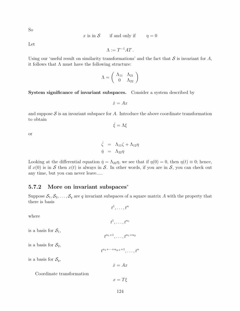
So

x is in S if and only if η = 0

Let

Λ := T−1AT .

Using our ‘useful result on similarity transformations’ and the fact that S is invariant for A,it follows that Λ must have the following structure:

Λ =

(Λ11 Λ21

0 Λ22

)

System significance of invariant subspaces. Consider a system described by

x = Ax

and suppose S is an invariant subspace for A. Introduce the above coordinate transformationto obtain

ξ = Λξ

or

ζ = Λ11ζ + Λ12η

η = Λ22η

Looking at the differential equation η = Λ22η, we see that if η(0) = 0, then η(t) ≡ 0; hence,if x(0) is in S then x(t) is always in S. In other words, if you are in S, you can check outany time, but you can never leave.....

5.7.2 More on invariant subspaces∗

Suppose S1,S2, . . . ,Sq are q invariant subspaces of a square matrix A with the property thatthere is basis

t1, . . . , tn

where

t1, . . . , tn1

is a basis for S1,

tn1+1, . . . , tn1+n2

is a basis for S2,

tn1+···+nq−1+1, . . . , tn

is a basis for Sq,

x = Ax

Coordinate transformation

x = Tξ

124

whereT =

(t1 t2 . . . tn

)

that is, ti is the i-th column of T . Consider

Λ = T−1AT

Claim:Λ = blockdiag (Λ1, . . . , Λq)

125

5.8 Diagonalizable systems

5.8.1 Diagonalizable matrices

We say that a square matrix A is diagonalizable if it is similar to a diagonal matrix, that is,there is an invertible matrix T and a diagonal matrix Λ such that

Λ = T−1AT .

In this section, we show that A is diagonalizable if and only if it has the following property:For each distinct eigenvalue of A,

geometric multiplicity = algebraic multiplicity

Recall that the geometric multiplicity of an eigenvalue is the dimension of its eigenspace,or equivalently, the maximum number of linearly independent eigenvectors associated withthat eigenvalue. An eigenvalue whose geometric multiplicity equals its algebraic multiplicityis call a nondefective eigenvalue. Otherwise, it is considered defective. A matrix with theproperty that all its eigenvalues are nondefective is called a nondefective matrix. Otherwise,it is considered defective. When is a matrix A nondefective? Some examples are:

(a) A has n distinct eigenvalues where A is n× n.

(b) A is hermitian that is, A∗ = A.

We first need the following result.

Fact 4 Suppose that geometric multiplicity equals algebraic multiplicity for each distincteigenvalue of a square matrix A. Then A has a basis of eigenvectors:

v1, v2, . . . , vn

Example 54

A =

(0 10 0

)

Theorem 2 Suppose that for each distinct eigenvalue of A, its geometric multiplicity is thesame as its algebraic multiplicity . Then A is similar to a diagonal matrix Λ whose diagonalelements are the eigenvalues of A. (If an eigenvalue has multiplicity m, it appears m timeson the diagonal of Λ)

Proof. LetT :=

(v1 v2 . . . vn

)

where v1, . . . , vn is a basis of eigenvectors for A. Let λi be the eigenvalue corresponding tovi. Then,

Avi = λivi

126

DefiningΛ := T−1AT

it follows from the ‘useful result on similarity transformations’ that

Λ = diag (λ1, λ2, . . . , λn)

:=

λ1 0 . . . 00 λ2 . . . 0...

. . ....

0 0 . . . λn

︸︷︷︸Complex Jordan form of A

So A is similar to the diagonal matrix Λ.

Example 55

A =

4 −2 −20 2 −20 −2 2

The characteristic polynomial of A is

p(s) = det(sI − A) = (s− 4)[(s− 2)(s− 2)− 4] = s(s− 4)2

So A has eigenvalues,λ1 = 0, λ2 = 4

with algebraic multiplicities 1 and 2.The equation (A− λI)v = 0 yields:

For λ1 = 0,

rref(A− λ1I) = rref

4 −2 −20 2 −20 −2 2

= rref

4 0 −40 2 −20 0 0

=

1 0 −10 1 −10 0 0

Hence, λ1 has geometric multiplicity 1 and its eigenspace is spanned by

v1 =

111

For λ2 = 4,

rref(A− λ2I) = rref

0 −2 −20 −2 −20 −2 −2

= rref

0 −2 −20 0 00 0 0

=

0 1 10 0 00 0 0

127

Hence, λ2 has geometric multiplicity 2 and its eigenspace is spanned by

v2 =

100

and v3 =

0−1

1

Since the geometric multiplicity of each eigenvalue is equal to its algebraic multiplicity,A is diagonalizable and its Jordan form is

Λ =

0 0 00 4 00 0 4

A quick check with MATLAB yields Λ = T−1AT where T = (v1v2v3).

5.8.2 Diagonalizable continuous-time systems

Consider a continuous-time systemx = Ax

and suppose A is an n × n diagonalizable matrix, that is, there is a nonsingular matrix Tsuch that

Λ = T−1AT

is diagonal. Hence, the diagonal elements of Λ are the eigenvalues (including possible mul-tiplicities) λ1, λ2, . . . , λn of A. Introducing the state transformation,

x = Tξ

we have ξ = T−1x and the system behavior is now equivalently described by

ξ = Λξ .

This yields

ξ1 = λ1ξ1

ξ2 = λ2ξ2...

ξn = λnξn

that is, n decoupled first order systems. Hence, for i = 1, 2, . . . , n,

ξi(t) = eλitξi0 (5.10)

where ξi0 = ξ(0). In vector form, we obtain

ξ(t) =

eλ1t 0 . . . 00 eλ2t . . . 0...

. . ....

0 0 . . . eλnt

ξ0 (5.11)

128

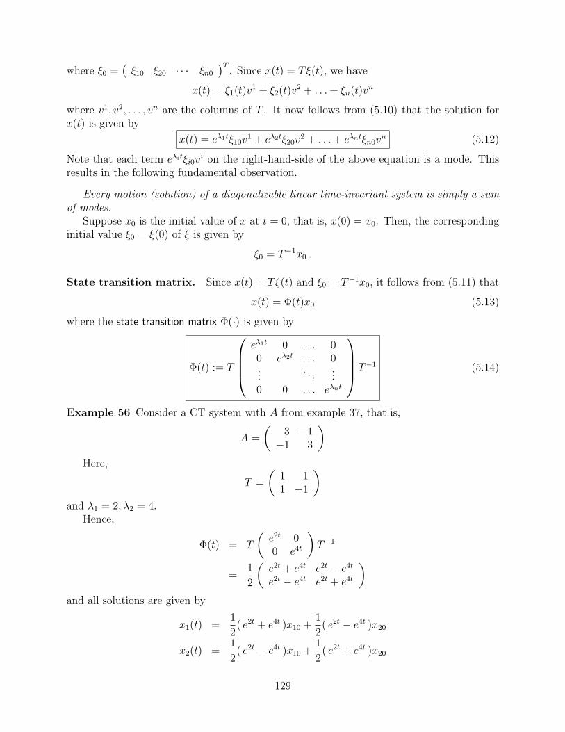
where ξ0 =(

ξ10 ξ20 · · · ξn0

)T. Since x(t) = Tξ(t), we have

x(t) = ξ1(t)v1 + ξ2(t)v

2 + . . . + ξn(t)vn

where v1, v2, . . . , vn are the columns of T . It now follows from (5.10) that the solution forx(t) is given by

x(t) = eλ1tξ10v1 + eλ2tξ20v

2 + . . . + eλntξn0vn (5.12)

Note that each term eλitξi0vi on the right-hand-side of the above equation is a mode. This

results in the following fundamental observation.

Every motion (solution) of a diagonalizable linear time-invariant system is simply a sumof modes.

Suppose x0 is the initial value of x at t = 0, that is, x(0) = x0. Then, the correspondinginitial value ξ0 = ξ(0) of ξ is given by

ξ0 = T−1x0 .

State transition matrix. Since x(t) = Tξ(t) and ξ0 = T−1x0, it follows from (5.11) that

x(t) = Φ(t)x0 (5.13)

where the state transition matrix Φ(·) is given by

Φ(t) := T

eλ1t 0 . . . 00 eλ2t . . . 0...

. . ....

0 0 . . . eλnt

T−1 (5.14)

Example 56 Consider a CT system with A from example 37, that is,

A =

(3 −1

−1 3

)

Here,

T =

(1 11 −1

)

and λ1 = 2, λ2 = 4.Hence,

Φ(t) = T

(e2t 00 e4t

)T−1

=1

2

(e2t + e4t e2t − e4t

e2t − e4t e2t + e4t

)

and all solutions are given by

x1(t) =1

2( e2t + e4t )x10 +

1

2( e2t − e4t )x20

x2(t) =1

2( e2t − e4t )x10 +

1

2( e2t + e4t )x20

129

Exercise 56 Compute the state transition matrix for the CT system corresponding to theA matrix in example 55.

5.8.3 Diagonalizable DT systems

The story here is basically the same as that for CT. Consider a DT system

x(k + 1) = Ax(k)

and suppose A is diagonalizable, that is, there is a nonsingular matrix T such that

Λ = T−1AT

is diagonal and the diagonal elements of Λ are the eigenvalues λ1, . . . , λn of A.Introducing the state transformation,

x = Tξ

we have ξ = T−1x and its behavior is described by:

ξ(k + 1) = Λξ(k)

Hence,

ξ1(k + 1) = λ1ξ1(k)

ξ2(k + 1) = λ2ξ2(k)...

ξn(k + 1) = λnξn(k)

Ifx(0) = x0

thenξ(0) = ξ0 = T−1x0

So,ξi(k) = λk

i ξi0, i = 1, 2, . . . , n

or,

ξ(k) =

λk1 0 . . . 00 λk

2 . . . 0...

. . ....

0 0 . . . λkn

ξ0

Sincex = ξ1v

1 + ξ2v2 + . . . + ξnv

n

130

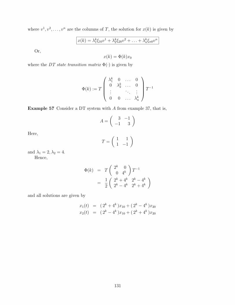
where v1, v2, . . . , vn are the columns of T , the solution for x(k) is given by

x(k) = λk1ξ10v

1 + λk2ξ20v

2 + . . . + λknξn0v

n

Or,x(k) = Φ(k)x0

where the DT state transition matrix Φ(·) is given by

Φ(k) := T

λk1 0 . . . 00 λk

2 . . . 0...

. . ....

0 0 . . . λkn

T−1

Example 57 Consider a DT system with A from example 37, that is,

A =

(3 −1

−1 3

)

Here,

T =

(1 11 −1

)

and λ1 = 2, λ2 = 4.Hence,

Φ(k) = T

(2k 00 4k

)T−1

=1

2

(2k + 4k 2k − 4k

2k − 4k 2k + 4k

)

and all solutions are given by

x1(t) = ( 2k + 4k )x10 + ( 2k − 4k )x20

x2(t) = ( 2k − 4k )x10 + ( 2k + 4k )x20

131

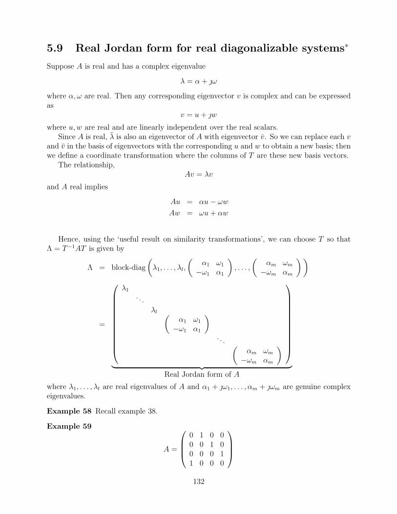
5.9 Real Jordan form for real diagonalizable systems∗

Suppose A is real and has a complex eigenvalue

λ = α + ω

where α, ω are real. Then any corresponding eigenvector v is complex and can be expressedas

v = u + w

where u,w are real and are linearly independent over the real scalars.Since A is real, λ is also an eigenvector of A with eigenvector v. So we can replace each v

and v in the basis of eigenvectors with the corresponding u and w to obtain a new basis; thenwe define a coordinate transformation where the columns of T are these new basis vectors.

The relationship,Av = λv

and A real implies

Au = αu− ωw

Aw = ωu + αw

Hence, using the ‘useful result on similarity transformations’, we can choose T so thatΛ = T−1AT is given by

Λ = block-diag

(λ1, . . . , λl,

(α1 ω1

−ω1 α1

), . . . ,

(αm ωm

−ωm αm

) )

=

λ1

. . .

λl (α1 ω1

−ω1 α1

)

. . . (αm ωm

−ωm αm

)

︸︷︷︸Real Jordan form of A

where λ1, . . . , λl are real eigenvalues of A and α1 + ω1, . . . , αm + ωm are genuine complexeigenvalues.

Example 58 Recall example 38.

Example 59

A =

0 1 0 00 0 1 00 0 0 11 0 0 0

132

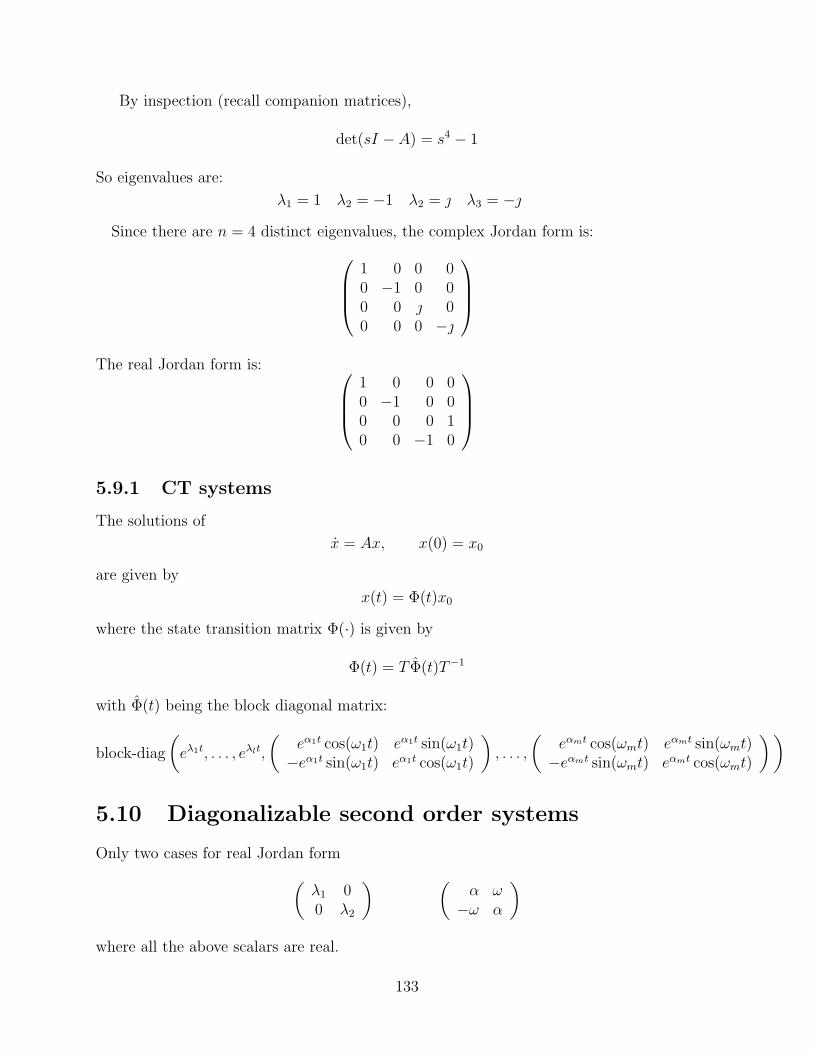
By inspection (recall companion matrices),

det(sI − A) = s4 − 1

So eigenvalues are:

λ1 = 1 λ2 = −1 λ2 = λ3 = −

Since there are n = 4 distinct eigenvalues, the complex Jordan form is:

1 0 0 00 −1 0 00 0 00 0 0 −

The real Jordan form is:

1 0 0 00 −1 0 00 0 0 10 0 −1 0

5.9.1 CT systems

The solutions of

x = Ax, x(0) = x0

are given by

x(t) = Φ(t)x0

where the state transition matrix Φ(·) is given by

Φ(t) = T Φ(t)T−1

with Φ(t) being the block diagonal matrix:

block-diag

(eλ1t, . . . , eλlt,

(eα1t cos(ω1t) eα1t sin(ω1t)−eα1t sin(ω1t) eα1t cos(ω1t)

), . . . ,

(eαmt cos(ωmt) eαmt sin(ωmt)−eαmt sin(ωmt) eαmt cos(ωmt)

))

5.10 Diagonalizable second order systems

Only two cases for real Jordan form

(λ1 00 λ2

) (α ω

−ω α

)

where all the above scalars are real.

133

5.10.1 State plane portraits for CT systems

Real eigenvalues

Genuine complex eigenvalues

5.11 Exercises

134

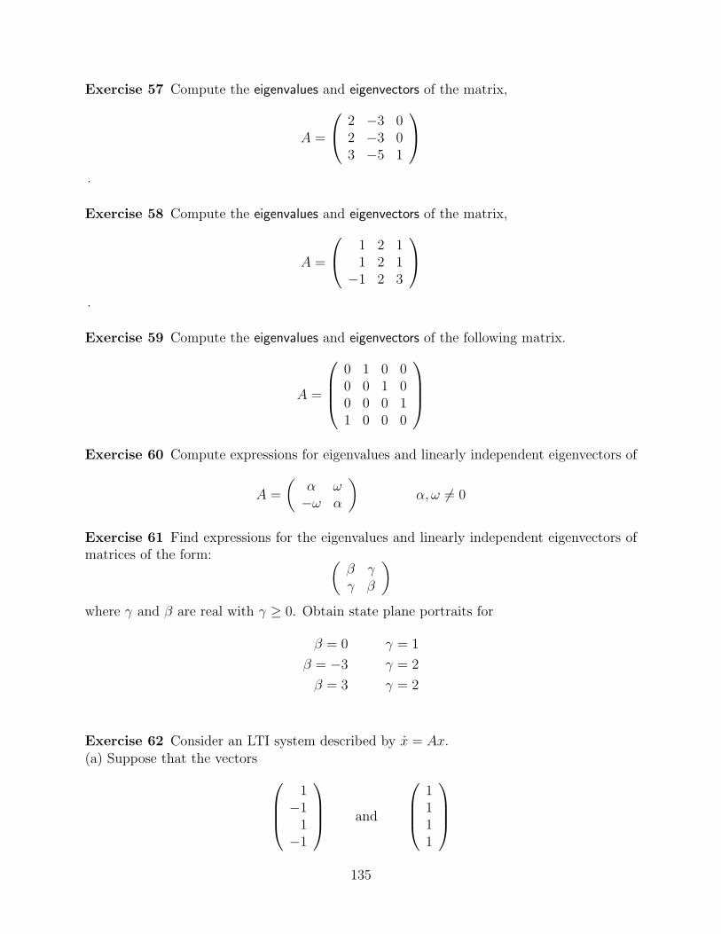
Exercise 57 Compute the eigenvalues and eigenvectors of the matrix,

A =

2 −3 02 −3 03 −5 1

.

Exercise 58 Compute the eigenvalues and eigenvectors of the matrix,

A =

1 2 11 2 1

−1 2 3

.

Exercise 59 Compute the eigenvalues and eigenvectors of the following matrix.

A =

0 1 0 00 0 1 00 0 0 11 0 0 0

Exercise 60 Compute expressions for eigenvalues and linearly independent eigenvectors of

A =

(α ω−ω α

)α, ω 6= 0

Exercise 61 Find expressions for the eigenvalues and linearly independent eigenvectors ofmatrices of the form: (

β γγ β

)

where γ and β are real with γ ≥ 0. Obtain state plane portraits for

β = 0 γ = 1

β = −3 γ = 2

β = 3 γ = 2

Exercise 62 Consider an LTI system described by x = Ax.(a) Suppose that the vectors

1−1

1−1

and

1111

135

are eigenvectors of A corresponding to eigenvalues −2 and 3, respectively. What is theresponse x(t) of the system to the initial condition

x(0) =

1010

?

(b) Suppose A is a real matrix and the vector

1

−1−

is an eigenvector of A corresponding to the eigenvalue 2 + 3ı. What is the response x(t) ofthe system to the initial condition

x(0) =

10

−10

?

Exercise 63 Suppose A is a square matrix and the vectors

123

and

111

are eigenvectors of A corresponding to eigenvalues −1 and 1, respectively. What is theresponse x(t) of the system x = Ax to the following initial conditions.

(a) x(0) =

246

(b) x(0) =

222

(c) x(0) =

024

?

(d) Suppose A is a real matrix and the vector

1 + 21−

3

is an eigenvector of A corresponding to the eigenvalue 2 − 3. What is the response x(t) ofthe system x = Ax to the initial condition

x(0) =

113

?

136

Exercise 64 Suppose A is a real square matrix and the vectors

1−1

1−1

1248

1

−1−

are eigenvectors of A corresponding to eigenvalues −1 and 2 and , respectively. What is theresponse x(t) of the system x = Ax to the following initial conditions.

(a) x(0) =

2−2

2−2

(b) x(0) =

−1−2−4−8

(c) x(0) =

0339

(d) x(0) =

11

−1−1

?

Exercise 65 Suppose A is a real square matrix with characteristic polynomial

p(s) = (s + 2)(s2 + 4)2

Suppose that all eigenvectors of A are nonzero multiples of

12340

,

01 + −01

or

01−

01

What is the solution to x = Ax with the following initial conditions.

(a) x(0) =

24680

, (b) x(0) =

01001

, (c) x(0) =

00101

(d) All all solutions of the system x = Ax bounded? Justify your answer.

Exercise 66 Consider a discrete-time LTI system described by x(k+1) = Ax(k).(a) Suppose that the vectors

1−1

1−1

and

1111

are eigenvectors of A corresponding to eigenvalues −2 and 3, respectively. What is theresponse x(k) of the system to the initial condition

x(0) =

1010

?

137

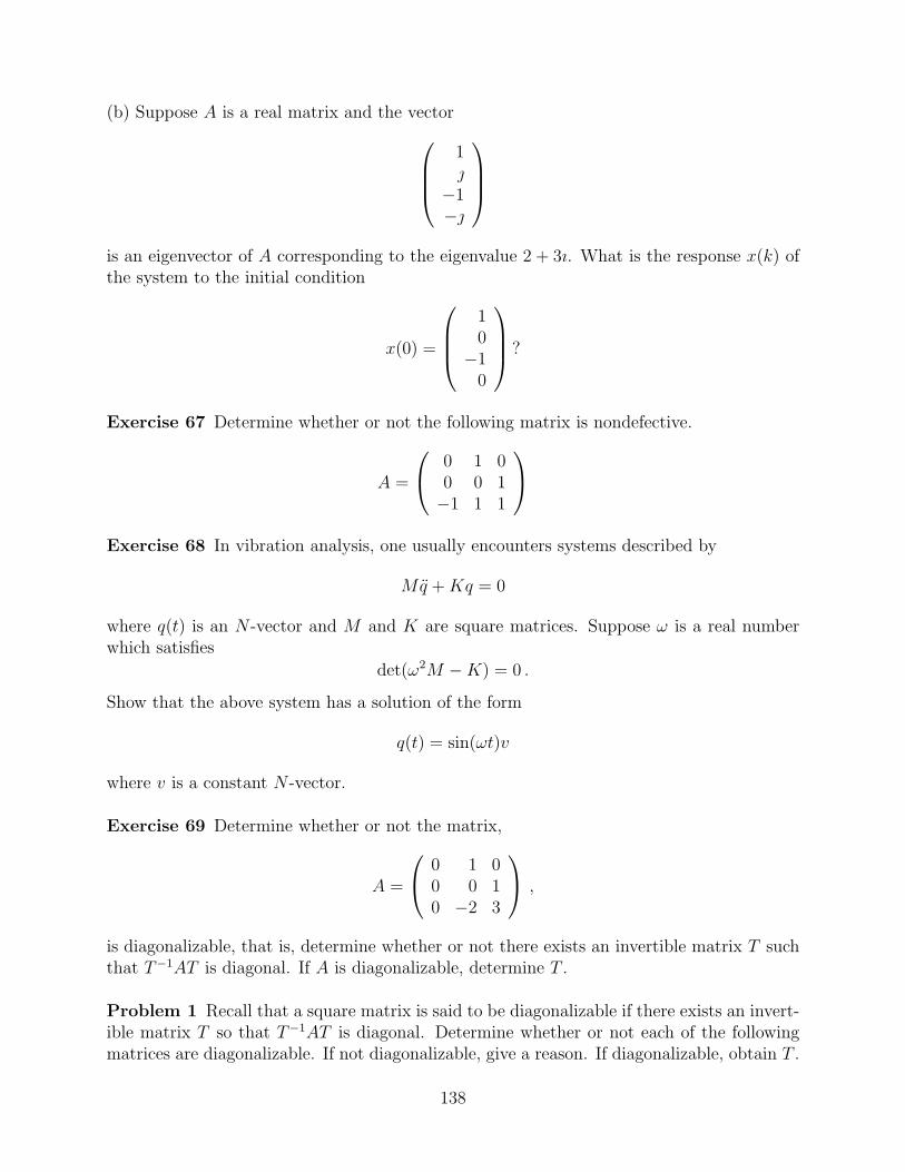
(b) Suppose A is a real matrix and the vector

1

−1−

is an eigenvector of A corresponding to the eigenvalue 2 + 3ı. What is the response x(k) ofthe system to the initial condition

x(0) =

10

−10

?

Exercise 67 Determine whether or not the following matrix is nondefective.

A =

0 1 00 0 1−1 1 1

Exercise 68 In vibration analysis, one usually encounters systems described by

Mq + Kq = 0

where q(t) is an N -vector and M and K are square matrices. Suppose ω is a real numberwhich satisfies

det(ω2M −K) = 0 .

Show that the above system has a solution of the form

q(t) = sin(ωt)v

where v is a constant N -vector.

Exercise 69 Determine whether or not the matrix,

A =

0 1 00 0 10 −2 3

,

is diagonalizable, that is, determine whether or not there exists an invertible matrix T suchthat T−1AT is diagonal. If A is diagonalizable, determine T .

Problem 1 Recall that a square matrix is said to be diagonalizable if there exists an invert-ible matrix T so that T−1AT is diagonal. Determine whether or not each of the followingmatrices are diagonalizable. If not diagonalizable, give a reason. If diagonalizable, obtain T .

138

(a)

A =

0 1 00 0 10 1 0

(b)

A =

(0 1

−1 2

)

(c)

A =

1 0 00 0 10 1 0

139

Chapter 6

eAt

Recall that all solutions to the scalar system x = ax satisfy x(t) = ea(t−t0)x(t0) for all t andt0. Recall also the power series expansion for eat:

eat = 1 + at +1

2!(at)2 + · · ·+ 1

k!(at)k + · · ·

The main result of this chapter is that all solutions of x = Ax satisfy

x(t) = eA(t−t0)x(t0) (6.1)

for all t and t0 where

eAt = 1 + At +1

2!(At)2 + · · ·+ 1

k!(At)k + · · · (6.2)

6.1 State transition matrix

6.1.1 Continuous time

Consider the initial value problem specified by

x = Ax and x(t0) = x0 . (6.3)

It can be shown that for each initial time t0 and each initial state x0 there is an uniquesolution x(·) to the above initial value problem and this solution is defined for all time t.Let φ(t; t0, x0) be the value of this solution at t, that is, for any t0 and x0, the solution to(6.3) is given by x(t) = φ(t; t0, x). Since the system x = Ax is time-invariant, we must haveφ(t; t0, x0) = φ(t−t0; x0) for some function φ. Since the system under consideration is linear,one can show that, for any t and t0, the solution at time t depends linearly on the initialstate x0 at time t0; hence there exists a matrix Φ(t−t0) such that φ(t−t0, x0) = Φ(t−t0)x0.We call the matrix valued function Φ(·) the state transition matrix for the system x = Ax.So, we have concluded that there is a matrix valued function Φ(·) such that for any t0 andx0, the solution x(·) to the above initial value problem is given by

x(t) = Φ(t−t0)x0

141

We now show that Φ must satisfy the following matrix differential equation and initialcondition:

Φ = AΦΦ(0) = I

To demonstrate this, consider any initial state x0 and let x(·) be the solution to (6.3)with t0 = 0. Then x(t) = Φ(t)x0. Considering t = 0, we note that

x0 = x(0) = Φ(0)x0 ;

that is Φ(0)x0 = x0. Since the above holds for any x0, we must have Φ(0) = I.We now note that for all t,

Φ(t)x0 = x(t) = Ax(t) = AΦ(t)x0 ;

that is Φ(t)x0 = AΦ(t)x0. Since the above must hold for any x0, we obtain that Φ(t) = AΦ(t).Note that the above two conditions on Φ uniquely specify Φ (Why?) The purpose of this

section is to examine Φ and look at ways of evaluating it.

142

6.1.2 Discrete time

x(k+1) = Ax(k) and x(k0) = x0

We havex(k) = Φ(k−k0)x0

The matrix valued function Φ(·) is called the state transition matrix and is given by

Φ(k) = Ak

Note that, if A is singular, Φ(k) is not defined for k < 0. That was easy; now for CT.

143

6.2 Polynomials of a square matrix

6.2.1 Polynomials of a matrix

We define polynomials of a matrix as follows. Consider any polynomial p of a scalar variables given by:

p(s) = a0 + a1s + a2s2 + . . . + amsm

where a0, . . . , am are scalars. If A is a square matrix, we define p(A) as follows:

p(A) := a0I + a1A + a2A2 + . . . + amAm

that is, we replace sk with Ak. (Recall that s0 = 1 and A0 = I)The following properties can be readily deduced from the above definition.

(a) The matrices A and p(A) commute, that is,

Ap(A) = p(A)A

(b) Consider any nonsingular matrix T , and suppose A = TΛT−1. Then

p(A) = Tp(Λ)T−1

(c) Suppose A is diagonal, that is,

A =

λ1 0 · · · 00 λ2 0...

. . ....

0 0 · · · λn

then

p(A) =

p(λ1) 0 · · · 00 p(λ2) 0...

. . ....

0 0 · · · p(λn)

(d) Suppose A is diagonalizable, that is, for some nonsingular T ,

A = T

λ1 0 · · · 00 λ2 0...

. . ....

0 0 · · · λn

T−1

Then

p(A) = T

p(λ1) 0 · · · 00 p(λ2) 0...

. . ....

0 0 · · · p(λn)

T−1

(e) If λ is an eigenvalue of A with eigenvector v, then p(λ) is an eigenvalue of p(A) witheigenvector v.

Properties (b)-(d) are useful for computing p(A).

144

Example 60 For

A =

(3 −1

−1 3

)

we found that

T =

(1 11 −1

)

results in

Λ = T−1AT =

(2 00 4

)

Hence, A = TΛT−1 and

p(A) = Tp(Λ)T−1

= T

(p(2) 00 p(4)

)T−1

=1

2

(p(2) + p(4) p(2)− p(4)p(2)− p(4) p(2) + p(4)

)

Suppose p is the characteristic polynomial of A. Since 2, 4 are the eigenvalues of A, we havep(2) = p(4) = 0; hence

p(A) = 0

6.2.2 Cayley-Hamilton Theorem

The following result is a fundamental result in linear algebra and is very useful in systemsand control.

Theorem 3 If p is the characteristic polynomial of a square matrix A, then

p(A) = 0 .

Proof. The proof is easy for a diagonalizable matrix A. Recall that such a matrix issimilar to a diagonal matrix whose diagonal elements λ1, . . . , λn are the eigenvalues of A;hence p(λ1) = . . . = p(λn) = 0. Now use property (d) above. We will leave the proof of thegeneral nondiagonalizable case for another day.

Suppose the characteristic polynomial of A is

det(sI − A) = a0 + a1s + . . . + an−1sn−1 + sn

Then the Cayley Hamilton theorem states that

a0I + a1A + . . . + an−1An−1 + An = 0

145

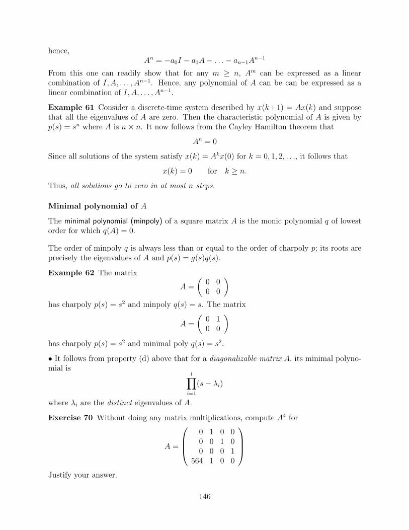
hence,An = −a0I − a1A− . . .− an−1A

n−1

From this one can readily show that for any m ≥ n, Am can be expressed as a linearcombination of I, A, . . . , An−1. Hence, any polynomial of A can be can be expressed as alinear combination of I, A, . . . , An−1.

Example 61 Consider a discrete-time system described by x(k+1) = Ax(k) and supposethat all the eigenvalues of A are zero. Then the characteristic polynomial of A is given byp(s) = sn where A is n× n. It now follows from the Cayley Hamilton theorem that

An = 0

Since all solutions of the system satisfy x(k) = Akx(0) for k = 0, 1, 2, . . ., it follows that

x(k) = 0 for k ≥ n.

Thus, all solutions go to zero in at most n steps.

Minimal polynomial of A

The minimal polynomial (minpoly) of a square matrix A is the monic polynomial q of lowestorder for which q(A) = 0.

The order of minpoly q is always less than or equal to the order of charpoly p; its roots areprecisely the eigenvalues of A and p(s) = g(s)q(s).

Example 62 The matrix

A =

(0 00 0

)

has charpoly p(s) = s2 and minpoly q(s) = s. The matrix

A =

(0 10 0

)

has charpoly p(s) = s2 and minimal poly q(s) = s2.

• It follows from property (d) above that for a diagonalizable matrix A, its minimal polyno-mial is

l∏i=1

(s− λi)

where λi are the distinct eigenvalues of A.

Exercise 70 Without doing any matrix multiplications, compute A4 for

A =

0 1 0 00 0 1 00 0 0 1

564 1 0 0

Justify your answer.

146

6.3 Functions of a square matrix

Consider a complex valued function f of a complex variable λ. Suppose f is analytic in someopen disk λ ∈ C : |λ| < ρ of radius ρ > 0. Then, provided |λ| < ρ, f(λ) can be expressedas the sum of a convergent power series; specifically

f(λ) =∞∑

k=0

akλk = a0 + a1λ + a2λ

2 + . . .

where

ak =1

k!f (k)(0) =

1

k!

dkf

dλk(0)

Suppose A is a square complex matrix and |λi| < ρ for every eigenvalue λi of A. Then,it can be shown that the power series ∑n

k=0 akAk∞n=0 is convergent. We define f(A) to be

the sum of this power series, that is,

f(A) :=∞∑

k=0

akAk = a0I + a1A + a2A

2 + . . .

Example 63 Consider

f(λ) =1

1− λ

This is analytic in the open unit disk (ρ = 1) and

f(λ) =∞∑

k=0

λk = 1 + λ + λ2 + . . .

Consider any matrix A with eigenvalues in the open unit disk. Then the series ∑nk=0 Ak∞n=0

is convergent and we let

f(A) :=∞∑

k=0

Ak

Multiplication of both sides of the above equality by I − A yields

(I − A)f(A) =∞∑

k=0

(Ak − Ak+1) = I;

hence the matrix I − A is invertible with inverse f(A) and we obtain the following powerseries expansion for (I − A)−1:

(I − A)−1 =∞∑

k=0

Ak = I + A + A2 + . . .

147

Power series expansion for (sI − A)−1. We present here an expansion which will beuseful later on. Consider any square matrix A and any complex number s which satisfies:

|s| > |λi| for every eigenvalue λi of A .

Then sI −A is invertible and (sI −A)−1 = 1s(I − 1

sA)−1. Also, the eigenvalues of 1

sA are in

the open unit disk; hence

(I − 1

sA)−1 =

∞∑

k=0

1

skAk = I +

1

sA +

1

s2A2 + . . .

and

(sI − A)−1 =∞∑

k=0

1

sk+1Ak =

1

sI +

1

s2A +

1

s3A2 + . . .

Properties of f(A). The following properties can be readily deduced from the abovedefinition of f(A).

(a) The matrices A and f(A) commute, that is,

Af(A) = f(A)A .

(b) Consider any nonsingular matrix T and suppose A = TΛT−1. Then

f(A) = Tf(Λ)T−1 .

(c) Suppose A is diagonal, that is,

A =

λ1 0 · · · 00 λ2 0...

. . ....

0 0 · · · λn

then

f(A) =

f(λ1) 0 · · · 00 f(λ2) 0...

. . ....

0 0 · · · f(λn)

(d) Suppose A is diagonalizable, that is, for some nonsingular T ,

A = T

λ1 0 · · · 00 λ2 0...

. . ....

0 0 · · · λn

T−1

148

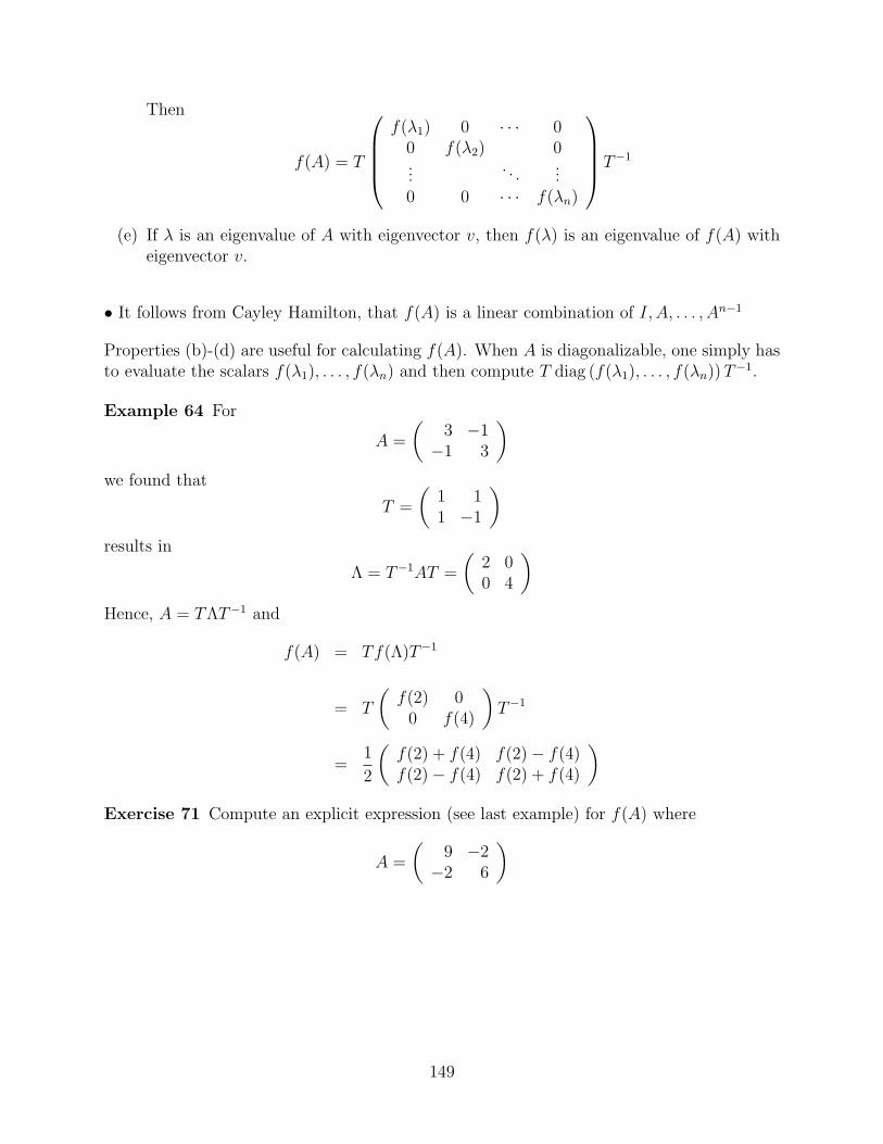
Then

f(A) = T

f(λ1) 0 · · · 00 f(λ2) 0...

. . ....

0 0 · · · f(λn)

T−1

(e) If λ is an eigenvalue of A with eigenvector v, then f(λ) is an eigenvalue of f(A) witheigenvector v.

• It follows from Cayley Hamilton, that f(A) is a linear combination of I, A, . . . , An−1

Properties (b)-(d) are useful for calculating f(A). When A is diagonalizable, one simply hasto evaluate the scalars f(λ1), . . . , f(λn) and then compute T diag (f(λ1), . . . , f(λn)) T−1.

Example 64 For

A =

(3 −1

−1 3

)

we found that

T =

(1 11 −1

)

results in

Λ = T−1AT =

(2 00 4

)

Hence, A = TΛT−1 and

f(A) = Tf(Λ)T−1

= T

(f(2) 0

0 f(4)

)T−1

=1

2

(f(2) + f(4) f(2)− f(4)f(2)− f(4) f(2) + f(4)

)

Exercise 71 Compute an explicit expression (see last example) for f(A) where

A =

(9 −2

−2 6

)

149

6.3.1 The matrix exponential: eA

Recall the exponential function:f(λ) = eλ

This function is analytic in the whole complex plane (that is ρ = ∞) and

dkeλ

dλk= eλ

for k = 1, 2, . . .; hence for any complex number λ,

eλ =∞∑

k=0

1

k!λk = 1 + λ +

1

2λ2 +

1

3!λ3 + . . .

Thus the exponential of any square matrix A is defined by:

eA :=∞∑

k=0

1

k!Ak = I + A +

1

2!A2 + . . .

and this power series converges for every square matrix A. Some properties:

(a) For any zero matrix 0,e0 = I

(b) Suppose t is a scalar variable.

deAt

dt= AeAt = eAtA

The following results also hold:

(i)eA(t1+t2) = eAt1eAt2

e−A = (eA)−1

(ii) If λ is an eigenvalue of A with eigenvector v, then eλ is an eigenvalue of eA witheigenvector v. So, eA has no eigenvalue at 0 and hence:

(iii) eA is nonsingular.

(iv) The following result also holds

eA+B = eAeB if A and B commute

6.3.2 Other matrix functions

cos(A)

sin(A)

150

6.4 The state transition matrix: eAt

Using the above definitions and abusing notation (eAt instead of etA),

eAt :=∞∑

k=0

1

k!(tA)k = I + tA +

1

2!(tA)2 +

1

3!(tA)3 + . . .

LettingΦ(t) := eAt

we have

Φ(0) = I

Φ = AΦ

Hence, the solution ofx = Ax x(0) = x0

is given by

x(t) = eAtx0

151

6.5 Computation of eAt

6.5.1 MATLAB

>> help expm

EXPM Matrix exponential.

EXPM(X) is the matrix exponential of X. EXPM is computed using

a scaling and squaring algorithm with a Pade approximation.

Although it is not computed this way, if X has a full set

of eigenvectors V with corresponding eigenvalues D, then

[V,D] = EIG(X) and EXPM(X) = V*diag(exp(diag(D)))/V.

See EXPM1, EXPM2 and EXPM3 for alternative methods.

EXP(X) (that’s without the M) does it element-by-element.

6.5.2 Numerical simulation

Let φi be the i-th column of the state transition matrix Φ(t) = eAt; thus

Φ(t) =(

φ1(t) φ2(t) · · · φn(t))

.

Let x be the unique solution to x = Ax and x(0) = x0. Since x(t) = Φ(t)x0 we have

x(t) = x01φ1(t) + · · ·+ x0nφn

where x0i is the i-th component of x0. Hence φi, is the solution to

x = Ax x(0) = ei

where ei is all zeros except for its i-th component which is 1.

6.5.3 Jordan form

eAt = TeΛtT−1

where Λ = T−1AT and Λ is the Jordan form of A. We have already seen this for diagonal-izable systems.

6.5.4 Laplace style

x = Ax x(0) = x0

152

SupposeX(s) = L(x)(s)

is the Laplace transform of x(·) evaluated at s ∈ C. Taking the Laplace transform of x = Axyields:

sX(s)− x0 = AX(s)

Hence, except when s is an eigenvalue of A, sI − A is invertible and

L(x)(s) = X(s) = (sI − A)−1x0

Since x(t) = eAtx0 for all x0, we must have

L(eAt) = (sI − A)−1

eAt = L−1 ((sI − A)−1)

Example 65 Recall

A =

(3 −1

−1 3

)

So,

(sI − A)−1 =

s−3(s−2)(s−4)

−1(s−2)(s−4)

−1(s−2)(s−4)

s−3(s−2)(s−4)

Since

s− 3

(s− 2)(s− 4)=

1

2

(1

s− 2+

1

s− 4

)

−1

(s− 2)(s− 4)=

1

2

(1

s− 2− 1

s− 4

)

and

L−1(1

s− 2) = e2t L−1(

1

s− 4) = e4t

we have,

eAt = L−1((sI − A)−1

)

=1

2

(e2t + e4t e2t − e4t

e2t − e4t e2t + e4t

)

Exercise 72 Compute eAt at t = ln(2) for

A =

(0 11 0

)

using all methods of this section.

153

6.6 Sampled-data systems

Here we discuss the process of discretizing a continuous-time system to obtain a discrete-timesystem.

Consider a continuous-time LTI system described by

xc(t) = Acxc(t) .

Suppose we only look at the behavior of this system at discrete instants of time, namely

· · · ,−2T, T, 0, T, 2T, · · ·where T > 0 is called the sampling time.

Figure 6.1: Sampling

If we introduce the discrete-time state defined

xd(k) = xc(kT ) k = . . . ,−2,−1, 0, 1, 2, . . . ,

then,

xd(k+1) = xc( (k+1)T )

= eAcT xc(kT )

= eAcT xd(k)

Hence, this sampled data system is described by the discrete-time system

xd(k+1) = Adxd(k)

whereAd = eAcT

154

The eigenvalues of Ad areeλ1T , . . . eλlT

where λ1, . . . , λl are the eigenvalues of Ac. Note that,

|eλiT | < 1 iff <(λi) < 0

|eλiT | = 1 iff <(λi) = 0

|eλiT | > 1 iff <(λi) > 0

eλiT = 1 iff λi = 0

It should be clear that all eigenvalues of Ad are nonzero, that is Ad in invertible.

Note that if we approximate eAcT by the first two terms in its power series, that is,

eAcT ≈ I + AcT

then,Ad ≈ I + AcT .

6.7 Exercises

Exercise 73 Suppose A is a 3× 3 matrix, b is a 3-vector and

det(sI − A) = s3 + 2s2 + s + 1

(a) Express A3b in terms of b, Ab, A2b.

(b) Suppose that the matrix

T =(

b Ab A2b)

is invertible. What is the matrix Λ := T−1AT? Specify each element of Λ explicitly.

Exercise 74 Suppose A is a 3× 3 matrix and

det(sI − A) = s3 + 2s2 + s + 1

(a) Express A3 in terms of I, A, A2.

(b) Express A5 in terms of I, A, A2.

(c) Express A−1 in terms of I, A, A2

Exercise 75 Suppose A is a 3× 3 matrix with eigenvalues 1, 2π and −2π. What are theeigenvalues of eA.

155

Exercise 76 Consider the differential equation

x = Ax (6.4)

where A is a square matrix. Show that if A has 2π as an eigenvalue, then there is an nonzeroinitial state x0 such that (6.4) has a solution x which satisfies x(1) = x(0) = x0.

Exercise 77 Suppose A is a square matrix.(a) Obtain expressions for

cos(At) and sin(At) .

(b) Show that

cos(At) = (eAt + e−At)/2 and sin(At) = (eAt − e−At)/2

(c) Show that

d cos(At)

dt= −A sin(At) and

d sin(At)

dt= A cos(At) .

Exercise 78 Compute eAt for the matrix

A =

(3 −5

−5 3

)

Exercise 79 Compute eAt for the matrix,

A =

( −11 20−6 11

).


A =

(0 11 0

)

Exercise 81 Suppose A is a matrix with four distinct eigenvalues: −1, +1− j, j. Show thatA4 = I.

Exercise 82 Suppose

A =

0 1 0 00 0 1 00 0 0 10 0 0 0

What is A20 + 4A4?

Exercise 83 Compute eAt for the matrix,

A =

( −3 2−4 3

).

156


A =

(3 −5

−5 3

)

Exercise 85 Compute eAt at t = ln(2) for

A =

(0 1

−1 0

)

using all four methods mentioned in the notes.

157

Chapter 7

Stability and boundedness

Consider a general nonlinear system described by

x = f(x) (7.1)

where x(t) is a real n-vector and t is a real scalar. By a solution of (7.1) we mean anycontinuous function x(·) : [0, t1) → IRn with t1 > 0, which satisfies x(t) = f(x(t)) for0 ≤ t < t1.

7.1 Boundedness of solutions

DEFN. (Boundedness) A solution x(·) is bounded if there exists β ≥ 0 such that

||x(t)|| ≤ β for all t ≥ 0

A solution is unbounded if it is not bounded.

It should be clear from the above definitions that a solution x(·) is bounded if and onlyif each component xi(·) of x(·) is bounded. Also, a solution is unbounded if and only ifat least one of its components is unbounded. So, x(t) = [ e−t e−2t ]T is bounded whilex(t) = [ e−t et ]T is unbounded.

Example 66 All solutions of

x = 0

are bounded.

Example 67 All solutions of

x = x− x3

are bounded.

159

Example 68 All solutions (except the zero solution) of

x = x

are unbounded.

Example 69 Considerx = x2 , x(0) = x0

If x0 > 0, the corresponding solution has a finite escape time and is unbounded. If x0 < 0,the corresponding solution is bounded.

Example 70 Undamped oscillator.

x1 = x2

x2 = −x1

All solutions are bounded.

Boundedness and linear time-invariant systems. Consider a general LTI (linear time-invariant) system

x = Ax (7.2)

Recall that every solution of this system has the form

x(t) =l∑

i=1

ni−1∑j=0

tjeλitvij

where λ1, . . . , λl are the eigenvalues of A, ni is the index of λi, and the constant vectors vij

depend on initial state.We say that an eigenvalue λ of A is non-defective if its index is one; this means that the

algebraic multiplicity and the geometric multiplicity of λ are the same. Otherwise we say λis defective.

Hence we conclude that all solutions of (7.2) are bounded if and only if for each eigenvalueλi of A:

(b1) <(λi) ≤ 0 and

(b2) if <(λi) = 0 then λi is non-defective.

If there is an eigenvalue λi of A such that either

(u1) <(λi) > 0 or

(u2) <(λi) = 0 and λi is defective

then, the system has some unbounded solutions.

160


x1 = x2

x2 = 0

Here

A =

(0 10 0

)

has a single eigenvalue 0. This eigenvalue has algebraic multiplicity 2 but geometric multi-plicity 1; hence some of the solutions of the system are unbounded. One example is

x(t) =

(t1

)

Example 72

x1 = 0

x2 = 0

Here

A =

(0 00 0

)

has a single eigenvalue 0. This eigenvalue has algebraic multiplicity 2 and geometric mul-tiplicity 2. Hence all the solutions of the system are bounded. Actually every state is anequilibrium state and every solution is constant.

Example 73 (Resonance) Consider a simple linear oscillator subject to a sinusoidal inputof amplitude W :

q + q = W sin(ωt+φ)

Resonance occurs when ω = 1. To see this, let

x1 := q , x2 := q , x3 := W sin(ωt+φ) , x4 := ωW cos(ωt+φ)

to yieldx = Ax

where

A =

0 1 0 0−1 0 1 0

0 0 0 10 0 −ω2 0

If ω = 1 then, A has eigenvalues and −. These eigenvalues have algebraic multiplicity twobut geometric multiplicity one; hence the system has unbounded solutions.

161

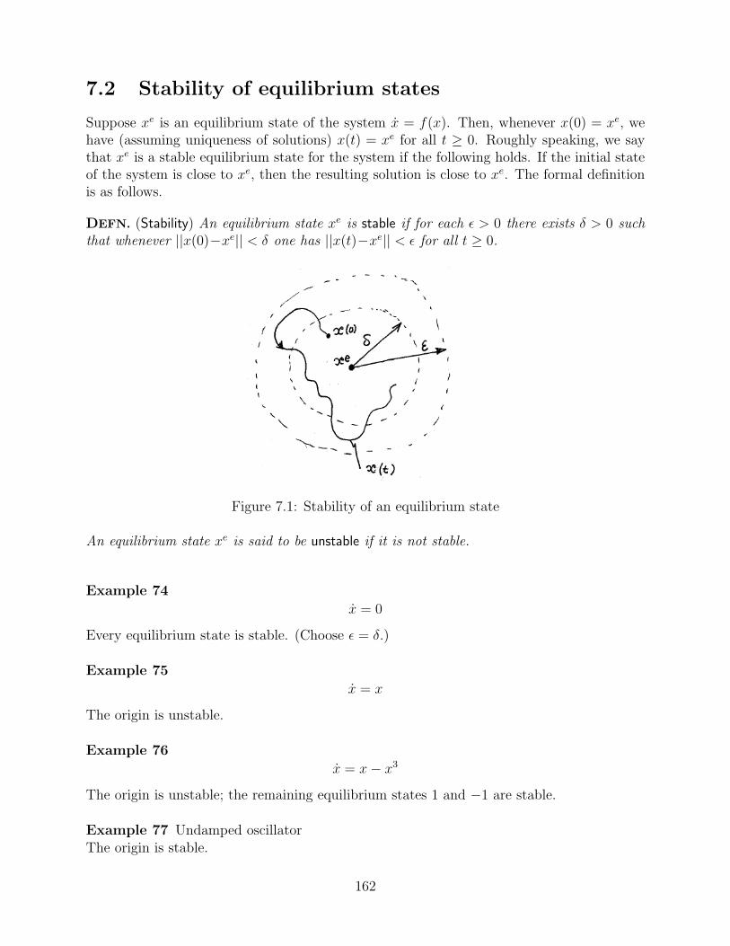
7.2 Stability of equilibrium states

Suppose xe is an equilibrium state of the system x = f(x). Then, whenever x(0) = xe, wehave (assuming uniqueness of solutions) x(t) = xe for all t ≥ 0. Roughly speaking, we saythat xe is a stable equilibrium state for the system if the following holds. If the initial stateof the system is close to xe, then the resulting solution is close to xe. The formal definitionis as follows.

DEFN. (Stability) An equilibrium state xe is stable if for each ε > 0 there exists δ > 0 suchthat whenever ||x(0)−xe|| < δ one has ||x(t)−xe|| < ε for all t ≥ 0.

Figure 7.1: Stability of an equilibrium state

An equilibrium state xe is said to be unstable if it is not stable.

Example 74

x = 0

Every equilibrium state is stable. (Choose ε = δ.)

Example 75

x = x

The origin is unstable.

Example 76

x = x− x3

The origin is unstable; the remaining equilibrium states 1 and −1 are stable.

Example 77 Undamped oscillatorThe origin is stable.

162

Example 78 Simple pendulum

x1 = x2

x2 = − sin x1

(0, 0) is stable; (π, 0) is unstable.

Example 79 Van der Pol oscillator

x1 = x2

x2 = (1− x21)x2 − x1

Figure 7.2: Van der Pol oscillator

The origin is unstable. However, all solutions are bounded.

Stability of linear time-invariant systems. It can be shown that every equilibriumstate of a LTI system (7.2) is stable if and only if all eigenvalues λi of A satisfy conditions(b1) and (b2) above. Hence every equilibrium state of a LTI system is stable if and only ifall solutions are bounded.It can also be shown that every equilibrium state is unstable if and only if there is aneigenvalue λi of A which satisfies condition (u1) or (u2) above. Hence every equilibriumstate of a LTI system is unstable if and only if there are unbounded solutions.

163

7.3 Asymptotic stability

7.3.1 Global asymptotic stability

DEFN. (Global asymptotic stability) An equilibrium state xe is globally asymptotically stable(GAS) if

(a) It is stable

(b) Every solution x(·) converges to xe with increasing time, that is,

limt→∞

x(t) = xe

If xe is a globally asymptotically stable equilibrium state, then there are no other equi-librium states and all solutions are bounded. In this case we say that the system x = f(x)is globally asymptotically stable.

Example 80 The systemx = −x

is GAS.

Example 81 The systemx = −x3

is GAS.

7.3.2 Asymptotic stability

In asymptotic stability, we do not require that all solutions converge to the equilibrium state;we only require that all solutions which originate in some neighborhood of the equilibriumstate converge to the equilibrium state.

DEFN. (Asymptotic stability) An equilibrium state xe is asymptotically stable (AS) if

(a) It is stable.

(b) There exists R > 0 such that whenever ||x(0)−xe|| < R one has

limt→∞

x(t) = xe . (7.3)

The region of attraction of an equilibrium state xe which is AS is the set of initial stateswhich result in (7.3), that is it is the set of initial states which are attracted to xe. Thus, theregion of attraction of a globally asymptotically equilibrium state is the whole state space.

164

Figure 7.3: Asymptotic stability

Example 82x = −x

Example 83x = x− x3

The equilibrium states −1 and 1 are AS with regions of attraction (−∞, 0) and (0,∞),respectively.

Example 84 Damped simple pendulum

x1 = x2

x2 = − sin x1 − x2

The zero state is AS but not GAS.

Example 85 Reverse Van der Pol oscillator

x1 = −x2

x2 = −(1− x21)x2 + x1

The zero state is AS but not GAS. Also, the system has unbounded solutions.

Figure 7.4: Reverse Van der Pol oscillator

165

LTI systems. For LTI systems, it should be clear from the general form of the solutionthat the zero state is AS if and only if all the eigenvalues λi of A have negative real parts,that is,

<(λi) < 0

Also AS is equivalent to GAS.

Example 86 The system

x1 = −x1 + x2

x2 = −x2

is GAS.


x1 = −x1 + x2

x2 = −x1 − x2

is GAS.

7.4 Exponential stability

We now present the “strongest” form of stability considered in this section.

DEFN. (Global exponential stability) An equilibrium state xe is globally exponentially stable(GES) with rate of convergence α > 0 if there exists β > 0 such that every solution satisfies

||x(t)−xe|| ≤ β||x(0)−xe|| exp(−αt) for all t ≥ 0

Example 88x = −x

GES with rate α = 1.

Note that global exponential stability implies global asymptotic stability, but, in general,the converse is not true. This is illustrated in the next example. For linear time-invariantsystems, GAS and GES are equivalent.

Example 89x = −x3

Solutions satisfy

x(t) =x0√

1 + 2x20t

where x0 = x(0) .

GAS but not GES

166

DEFN. (Exponential stability) An equilibrium state xe is exponentially stable (ES) with rate ofconvergence α > 0 if there exists R > 0 and β > 0 such that whenever ||x(0)−xe|| < R onehas

||x(t)−xe|| ≤ β||x(0)−xe|| exp(−αt) for all t ≥ 0

Figure 7.5: Exponential stability

Note that exponential stability implies asymptotic stability, but, in general, the converse isnot true.

Example 90x = −x3

GAS but not even ES

Example 91

x = − x

1 + x2

GAS, ES, but not GES

7.5 LTI systems

Consider a LTI systemx = Ax (7.4)

Recall that every solution of this system has the form

x(t) =l∑

i=1

ni−1∑j=0

tjeλitvij

where λ1, . . . , λl are the eigenvalues of A, the integer ni is the index of λi, and the constantvectors vij depend on initial state. From this it follows that the stability properties of thissystem are completely determined by the location of its eigenvalues; this is summarized inthe table below.

167

The following table summarizes the relationhip between the stability properties of a LTIsystem and the eigenproperties of its A-matrix. In the table, unless otherwise stated, aproperty involving λ must hold for all eigenvalues λ of A.

Stability properties Eigenproperties

Global exponential stability <(λ) < 0and boundedness

Stability and <(λ) ≤ 0boundedness If <(λ) = 0 then λ is non-defective.

Instability and some There is an eigenvalue λ with <(λ) > 0 orunbounded solutions <(λ) = 0 and λ is defective.


x1 = −x1 + x2

x2 = −x2

is GES.


x1 = −x1 + x2

x2 = −x1 − x2

is GES.


x1 = 0

x2 = 0

is stable about every equilibrium point.


x1 = x2

x2 = 0

is unstable about every equilibrium point.

168

Figure 7.6: The big picture. For LTI systems, the concepts in each dashed box are equivalent

169

7.6 Linearization and stability

Consider a nonlinear time-invariant system described by

x = f(x)

where x(t) is an n-vector at each time t. Suppose xe is an equilibrium state for this system,that is, f(xe) = 0, and consider the linearization of this system about xe:

δx = Aδx where A =∂f

∂x(xe) .

The following results can be demonstrated using nonlinear Lyapunov stability theory.

Stability. If all the eigenvalues of the A matrix of the linearized system have negative realparts, then the nonlinear system is exponentially stable about xe.

Instability. If at least one eigenvalue of the A matrix of the linearized system has a positivereal part, then the nonlinear system is unstable about xe.

Undetermined. Suppose all the eigenvalues of the A matrix of the linearized system havenon-positive real parts and at least one eigenvalue of A has zero real part. Then, based onthe linearized system alone, one cannot predict the stability properties of the nonlinear systemabout xe.

Note that the first statement above is equivalent to the following statement. If thelinearized system is exponentially stable, then the nonlinear system is exponentially stableabout xe.

Example 96 (Damped simple pendulum.) Physically, the system

x1 = x2

x2 = − sin x1 − x2

has two distinct equilibrium states: (0, 0) and (π, 0). The A matrix for the linearization ofthis system about (0, 0) is

A =

(0 1

−1 −1

)

Since all the eigenvalues of this matrix have negative real parts, the nonlinear system isexponentially stable about (0, 0). The A matrix corresponding to linearization about (π, 0)is

A =

(0 11 −1

)

Since this matrix has an eigenvalue with a positive real part, the nonlinear system is unstableabout (π, 0)

The following example illustrates the fact that if the eigenvalues of the A matrix have non-positive real parts and there is at least one eigenvalue with zero real part, then, one cannotmake any conclusions on the stability of the nonlinear system based on the linearization.

170

Example 97 Consider the scalar nonlinear system:

x = ax3

This origin is GAS if a < 0, unstable if a > 0 and stable if a = 0. However, the linearizationof this system about zero, given by

δx = 0

is independent of a and is stable.

The following example illustrates that instability of the linearized system does not implyinstability of the nonlinear system.

Example 98 Using nonlinear techniques, one can show that the following system is GASabout the origin.

x1 = x2

x2 = −x31 − x3

2

However, the linearization of this system, given by

δx1 = δx2

δx2 = 0 ,

is unstable about the origin.

171

Exercises

Exercise 86 For each of the following systems, determine (from the state portrait) thestability properties of each equilibrium state. For AS equilibrium states, give the region ofattraction.

(a)x = −x− x3

(b)x = −x + x3

(c)x = x− 2x2 + x3

Exercise 87 If possible, use linearization to determine the stability properties of each ofthe following systems about the zero equilibrium state.

(i)

x1 = (1 + x21)x2

x2 = −x31

(ii)

x1 = sin x2

x2 = (cos x1)x3

x3 = ex1x2

Exercise 88 If possible, use linearization to determine the stability properties of each equi-librium state of the Lorenz system.

172

Chapter 8

Stability and boundedness: discretetime

8.1 Boundedness of solutions

Consider a general discrete-time nonlinear system described by

x(k+1) = f(x(k)) (8.1)

where x(k) is an n-vector and k is an integer. By a solution of (8.1) we mean a sequencex(·) = ( x(0), x(1), x(2), . . . ) which satisfies (8.1) for all k ≥ 0.

DEFN. (Boundedness of solutions) A solution x(·) is bounded if there exists β ≥ 0 such that

||x(k)|| ≤ β for all k ≥ 0 .

A solution is unbounded if it is not bounded.

It should be clear from the above definitions that a solution x(·) is bounded if and onlyif each component xi(·) of x(·) is bounded. Also, a solution is unbounded if and only if atleast one of its components is unbounded. So, x(k) = [ (0.5)k (−0.5)k ]T is bounded whilex(k) = [ (0.5)k 2k ]T is unbounded.

Example 99x(k+1) = 0


Example 100x(k+1) = x(k)


Example 101x(k+1) = −2x(k)

All solutions (except the zero solution) are unbounded.

173

Linear time invariant (LTI) systems. All solutions of the LTI system

x(k+1) = Ax(k) (8.2)

are bounded if and only if for each eigenvalue λ of A:

(b1) |λ| ≤ 1 and

(b2) if |λ| = 1 then λ is non-defective.

If there is an eigenvalue λ of A such that either

(u1) |λ| > 1 or

(u2) |λ| = 1 and λ is defective.

then the system has some unbounded solutions.

Example 102 Discrete unattached mass. Here

A =

(1 10 1

)

has a single eigenvalue 1. This eigenvalue has algebraic multiplicity 2 but geometric mul-tiplicity 1; hence this eigenvalue is defective. So, some of the solutions of the systemx(k+1) = Ax(k) are unbounded. One example is

x(k) =

(k1

)

8.2 Stability of equilibrium states

Suppose xe is an equilibrium state of the system x(k +1) = f(x(k)). Then, wheneverx(0) = xe, we have x(k) = xe for all k ≥ 0. Roughly speaking, we say that xe is a stableequilibrium state for the system if the following holds. If the initial state of the system isclose to xe, then the resulting solution is close to xe. The formal definition is as follows.

DEFN. (Stability) An equilibrium state xe is stable if for each ε > 0 there exists δ > 0 suchthat whenever ||x(0)−xe|| < δ, one has ||x(k)−xe|| < ε for all k ≥ 0.xe is unstable if it is not stable.

Example 103x(k+1) = −x(k) .

The origin is stable. (Consider δ = ε.)

Example 104x(k+1) = −2x(k) .

The origin is unstable.

Example 105x(k+1) = −x(k)3 .

The single equilibrium at the origin is stable, but, the system has unbounded solutions.

174

LTI systems. Every equilibrium state of a LTI system (8.2) is stable if and only if alleigenvalues λ of A satisfy conditions (b1) and (b2) above. Hence every equilibrium state ofa LTI system is stable if and only if all solutions are bounded.

Every equilibrium state is unstable if and only if there is an eigenvalue λ of A whichsatisfies condition (u1) or (u2) above. Hence every equilibrium state of a LTI system isunstable if and only if there are unbounded solutions.


8.3.1 Global asymptotic stability

DEFN. (Global asymptotic stability (GAS)) An equilibrium state xe is globally asymptoticallystable (GAS) if

(a) It is stable

(b) Every solution x(·) converges to xe, that is,

limk→∞

x(k) = xe .

If xe is a globally asymptotically stable equilibrium state, then there are no other equi-librium states. In this case we say the system (8.1) is globally asymptotically stable.

Example 106

x(k+1) =1

2x(k)

GAS

Example 107

x(k+1) =x(k)

2 + x(k)2

8.3.2 Asymptotic stability

DEFN. (Asymptotic stability (AS)) An equilibrium state xe is asymptotically stable (AS) if

(a) It is stable

(b) There exists R > 0 such that whenever ||x(0)− xe|| < R one has

limk→∞

x(k) = xe (8.3)

175

The region of attraction of an equilibrium state xe which is AS is the set of initial stateswhich result in (8.3), that is it is the set of initial states which are attracted to xe. Thus, theregion of attraction of a globally asymptotically equilibrium state is the whole state space.

Example 108

x(k+1) = x(k)3

Origin is AS with region of attraction [−1 1].

LTI systems. For LTI systems, it should be clear from the general form of the solutionthat the zero state is AS if and only if all the eigenvalues λi of A have magnitude less thanone, that is,

|λi| < 1 .

Also AS is equivalent to GAS.


We now present the “strongest” form of stability considered in this section.

DEFN. (Global exponential stability) An equilibrium state xe is globally exponentially stable(GES) with there exists 0 ≤ λ < 1 and β > 0 such that every solution satisfies

||x(k)−xe|| ≤ βλk||x(0)−xe|| for all k ≥ 0

Example 109

x(k+1) =1

2x(k)

GES with γ = 12.

Note that global exponential stability implies global asymptotic stability, but, in general,the converse is not true. This is illustrated in the next example. For linear time-invariantsystems, GAS and GES are equivalent.

Lemma 1 Consider a system described by x(k+1) = f(x(k)) and suppose that for somescalar λ ≥ 0,

‖f(x)‖ ≤ λ‖x‖for all x. Then, every solution x(·) of the system satisfies

‖x(k)‖ ≤ λk‖x(0)‖

for all k ≥ 0. In particular, if λ < 1 then, the system is globally exponentially stable.

176

Example 110

x(k+1) =x(k)√

1 + 2x(k)2

Solutions satisfy

x(k) =x0√

1 + 2kx20

where x0 = x(0) .

GAS but not GES

DEFN. (Exponential stability) An equilibrium state xe is exponentially stable (ES) if thereexists R > 0, 0 ≤ λ < 1 and β > 0 such that whenever ||x(0)−xe|| < R one has

||x(k)−xe|| ≤ βλk||x(0)−xe|| for all k ≥ 1

Note that exponential stability implies asymptotic stability, but, in general, the converseis not true.

Example 111

x(k+1) =x(k)√

1 + 2x(k)2

Solutions satisfy

x(k) =x0√

1 + 2kx20

where x0 = x(0) .

GAS but not even ES

8.5 LTI systems

The following table summarizes the relationhip between the stability properties of a LTIsystem and the eigenproperties of its A-matrix. In the table, unless otherwise stated, aproperty involving λ must hold for all eigenvalues λ of A.

Stability properties eigenproperties

Asymptotic stability |λ| < 1and boundedness

Stability and |λ| ≤ 1boundedness If |λ| = 1 then λ is non-defective

Instability and some There is an eigenvalue of A withunbounded solutions |λ| > 1 or

|λ| = 1 and λ is defective

177

8.6 Linearization and stability

Consider a nonlinear time-invariant system described by

x(k+1) = f(x(k))

where x(k) is an n-vector at each time t. Suppose xe is an equilibrium state for this system,that is, f(xe) = xe, and consider the linearization of this system about xe:

δx(k+1) = Aδx(k) where A =∂f

∂x(xe) .

The following results can be demonstrated using nonlinear Lyapunov stability theory.

Stability. If all the eigenvalues of the A matrix of the linearized system have magnitude lessthan one, then the nonlinear system is exponentially stable about xe.

Instability. If at least one eigenvalue of the A matrix of the linearized system has magnitudegreater than one, then the nonlinear system is unstable about xe.

Undetermined. Suppose all the eigenvalues of the A matrix of the linearized system havemagnitude less than or equal to one and at least one eigenvalue of A has magnitude one.Then, based on the linearized system alone, one cannot predict the stability properties of thenonlinear system about xe.

Note that the first statement above is equivalent to the following statement. If thelinearized system is exponentially stable, then the nonlinear system is exponentially stableabout xe.

Example 112 (Newton’s method) Recall that Newton’s method for a scalar functioncan be described by

x(k+1) = x(k)− g(x(k))

g′(x(k))

Here

f(x) = x− g(x)

g′(x)

So,

f ′(x) = 1− 1 +g(x)g′′(x)

g′(x)2=

g(x)g′′(x)

g′(x)2.

At an equilibrium state xe, we have g(xe) = 0; hence f ′(xe) = 0 and the linearization aboutany equilibrium state is given by

δx(k+1) = 0 .

Thus, every equilibrium state is exponentially stable.

178

Chapter 9

Basic Lyapunov theory

Suppose we are interested in the stability properties of the system

x = f(x) (9.1)

where x(t) is a real n-vector at time t. If the system is linear, we can determine its stabilityproperties from the properties of the eigenvalues of the system matrix. What do we do fora nonlinear system? We could linearize about each equilibrium state and determine thestability properties of the resulting linearizations. Under certain conditions this will tell ussomething about the local stability properties of the nonlinear system about its equilibriumstates. However there are situations where linearization cannot be used to deduce even thelocal stability properties of the nonlinear system. Also, linearization tells us nothing aboutthe global stability properties of the nonlinear system.

In general, we cannot explicitly obtain solutions for nonlinear systems. Lyapunov theoryallows to say something about the stability properties of a system without knowing the formor structure of the solutions.

In this chapter, V is a scalar-valued function of the state, that is V : IRn → IR. SupposeV is continuously differentiable. Then, at any time t, the derivative of V along a solution x(·)of system (9.1) is given by

dV

dt(x(t)) = DV (x(t))x(t)

= DV (x(t))f(x(t))

where DV (x) is the derivative of V at x and is given by

DV (x) =(

∂V∂x1

(x) ∂V∂x2

(x) . . . ∂V∂xn

(x))

Note that

DV (x)f(x) =∂V

∂x1

(x)f1(x) +∂V

∂x2

(x)f2(x) + . . . +∂V

∂xn

(x)fn(x)

In what follows, if a condition involves DV , then it is implicitly assumed that V is continu-ously differentiable. Sometimes DV is denoted by

∂V

∂x.

179

Also, when the system under consideration is fixed, DV f is sometimes denoted by

V .

This a slight but convenient abuse of notation.

180

9.1 Stability

9.1.1 Locally positive definite functions

DEFN. (Locally positive definite function) A function V is locally positive definite (lpd) abouta point xe if

V (xe) = 0

and there is a scalar R > 0 such that

V (x) > 0 whenever x 6= xe and ||x− xe|| < R

Basically, a function is lpd about a point xe if it is zero at xe has a strict local minimumat xe.

Figure 9.1: A locally positive definite function

Example 113 (Scalar x) The following functions are lpd about zero.

V (x) = x2

V (x) = 1− e−x2

V (x) = 1− cos x

V (x) = x2 − x4

Example 114

V (x) = ||x||2= x2

1 + x22 + . . . + x2

n

Lpd about the origin.

Quadratic forms. Suppose P is a real n × n symmetric matrix and is positive definite.Consider the quadratic form defined by

V (x) = xT Px =n∑

i=1

n∑j=1

Pijxixj .

181

Clearly V (0) = 0. Recalling the definition of a positive definite matrix, it follows thatV (x) = xT Px > 0 for all nonzero x. Hence V is locally positive definite about the origin.

• The second derivative of V at x is the square symmetric matrix given by:

D2V (x) :=

∂2V∂2x1

(x) ∂2V∂x1∂x2

(x) . . . ∂2V∂x1∂xn

(x)

∂2V∂x2∂x1

(x) ∂2V∂2x2

(x) . . . ∂2V∂x2∂xn

(x)

......

...

∂2V∂xn∂x1

(x) ∂2V∂xn∂x2

(x) . . . ∂2V∂2xn

(x)

that is,

D2V (x)ij =∂2V

∂xi∂xj

(x)

Sometimes D2V (x) is written as ∂2V∂x2 (x) and is referred to as the Hessian of V .

The following lemma is sometimes useful in demonstrating that a function is lpd.

Lemma 2 Suppose V is twice continuously differentiable and

V (xe) = 0

DV (xe) = 0

D2V (xe) > 0

Then V is a locally positive definite about xe.

Example 115 Consider V (x) = x2 − x4 where x is a scalar. Since V (0) = DV (0) = 0 andD2V (0) = 2 > 0, V is lpd about zero.

Example 116 Consider

V (x) = 1− cos x1 +1

2x2

2

ClearlyV (0) = 0

SinceDV (x) =

(sin x1 x2

)

we haveDV (0) = 0

Also,

D2V (x) =

(cos x1 0

0 1

)

182

Hence,

D2V (0) =

(1 00 1

)> 0

Since V satisfies the hypotheses of the previous lemma with xe = 0, it is lpd about zero.

9.1.2 A stability result

If the equilibrium state of a nonlinear system is stable but not asymptotically stable, thenone cannot deduce the stability properties of the equilibrium state of the nonlinear systemfrom the linearization of the nonlinear system about that equilibrium state

Theorem 4 (Stability) Suppose there exists a function V and a scalar R > 0 such that V islocally positive definite about xe and

DV (x)f(x) ≤ 0 for ||x− xe|| < R

Then xe is a stable equilibrium state.

If V satisfies the hypotheses of the above theorem, then V is said to be a Lyapunovfunction which guarantees the stability of xe.

Example 117x = 0

ConsiderV (x) = x2

as a candidate Lyapunov function. Then V is lpd about 0 and

DV (x)f(x) = 0

Hence (it follows from Theorem 4 that) the origin is stable.

Example 118 (Undamped linear oscillator.)

x1 = x2

x2 = −kx1 k > 0

Consider the total energy,

V (x) =1

2kx2

1 +1

2x2

2

as a candidate Lyapunov function. Then V is lpd about the origin and

DV (x)f(x) = 0

Hence the origin is stable.

183

Example 119 (Simple pendulum.)

x1 = x2

x2 = − sin x1

Consider the total energy,

V (x) = 1− cos x1 +1

2x2

2


DV (x)f(x) = 0

Hence the origin is stable

Example 120 (Stability of origin for attitude dynamics system.) Recall

x1 =(I2 − I3)

I1

x2x3

x2 =(I3 − I1)

I2

x3x1

x3 =(I1 − I2)

I3

x1x2

whereI1, I2, I3 > 0

Consider the kinetic energy

V (x) =1

2

(I1x

21 + I2x

22 + I3x

23

)


DV (x)f(x) = 0

Hence the origin is stable.

Example 121 (Undamped Duffing system)

x1 = x2

x2 = x1 − x31

As a candidate Lyapunov function for the equilibrium state xe = [ 1 0 ]T consider thetotal energy

V (x) =1

4x4

1 −1

2x2

1 +1

2x2

2 +1

4.

Since

DV (x) =(

x31 − x1 x2

)and D2V (x) =

(3x2

1 − 1 00 1

)

we have V (xe) = 0, DV (xe) = 0 and D2V (xe) > 0, and it follows that V is lpd about xe.One can readily verify that DV (x)f(x) = 0. Hence, xe is stable.

184

−3 −2 −1 0 1 2 3−3

−2

−1

0

1

2

3

y

ydot

Phase portrait of ddot y = y − y3

Figure 9.2: Duffing system

185

Exercises

Exercise 89 Determine whether or not the following functions are lpd. (a)

V (x) = x21 − x4

1 + x22

(b)V (x) = x1 + x2

2

(c)V (x) = 2x2

1 − x31 + x1x2 + x2

2

Exercise 90 (Simple pendulum with Coulomb damping.) By appropriate choice of Lya-punov function, show that the origin is a stable equilibrium state for

x1 = x2

x2 = − sin x1 − c sgm (x2)

where c > 0.

Exercise 91 By appropriate choice of Lyapunov function, show that the origin is a stableequilibrium state for

x1 = x2

x2 = −x31

Note that the linearization of this system about the origin is unstable.

Exercise 92 By appropriate choice of Lyapunov function, show that the origin is a stableequilibrium state for

x1 = x2

x2 = −x1 + x31

186


The following result presents conditions which guarantee that an equilibrium state is asymp-totically stable.

Theorem 5 (Asymptotic stability) Suppose there exists a function V and a scalar R > 0such that V is locally positive definite about xe and

DV (x)f(x) < 0 for x 6= xe and ||x− xe|| < R

Then xe is an asymptotically stable equilibrium state for x = f(x).

Example 122

x = −x3

Consider

V (x) = x2

Then V is lpd about zero and

DV (x)f(x) = −2x4 < 0 for x 6= 0

Hence the origin is AS.

Example 123

x = −x + x3

Consider

V (x) = x2


DV (x)f(x) = −2x2(1− x2) < 0 for |x| < 1, x 6= 0

Hence the origin is AS. Although the origin is AS, there are solutions which go unboundedin a finite time.

Example 124

x = − sin x

Consider

V (x) = x2


DV (x)f(x) = −2x sin(x) < 0 for |x| < π, x 6= 0


187

Example 125 (Simple pendulum with viscous damping.) Intuitively, we expect the originto be an asymptotically stable equilibrium state for the damped simple pendulum:

x1 = x2

x2 = − sin x1 − cx2

where c > 0 is the damping coefficient. If we consider the total mechanical energy

V (x) = 1− cos x1 +1

2x2

2

as a candidate Lyapunov function, we obtain

DV (x)f(x) = −cx22 .

Since DV (x)f(x) ≤ 0 for all x, we have stability of the origin. Since DV (x)f(x) = 0whenever x2 = 0, it follows that DV (x)f(x) = 0 for points arbitrarily close to the origin;hence V does not satisfy the requirements of the above theorem for asymptotic stability.

Suppose we modify V to

V (x) =1

2λc2x2

1 + λcx1x2 +1

2x2

2 + 1− cos x1

where λ is any scalar with 0 < λ < 1. Letting

P =1

2

(λc2 λcλc 1

)

note that P > 0 and

V (x) = xT Px + 1− cos x1

≥ xT Px

Hence V is lpd about zero and we obtain

DV (x)f(x) = −λcx1 sin x1 − (1− λ)cx22 < 0 for ||x|| < π, x 6= 0

to satisfy the requirements of above theorem; hence the origin is AS.

Exercises

Exercise 93 By appropriate choice of Lyapunov function, show that the origin is an asymp-totically stable equilibrium state for

x1 = x2

x2 = −x51 − x2

Exercise 94 By appropriate choice of Lyapunov function, show that the origin is a asymp-totically stable equilibrium state for

x1 = x2

x2 = −x1 + x31 − x2

188

9.3 Boundedness

9.3.1 Radially unbounded functions

DEFN. A scalar valued function V of the state x is said to be radially unbounded if

limx→∞

V (x) = ∞

Example 126V (x) = x2 yes

V (x) = 1− e−x2no

V (x) = x2 − x yesV (x) = x4 − x2 yesV (x) = x sin x noV (x) = x2(1− cos x) no

Example 127 Suppose P is a real n × n matrix and is positive definite symmetric andconsider the quadratic form defined by

V (x) = xT Px

Since P is real symmetric,xT Px ≥ λmin(P )||x||2

for all x, where λmin(P ) is the minimum eigenvalue of P . Since P is positive definite,λmin(P ) > 0. From this it should be clear that V is radially unbounded.

The following lemma can be useful for guaranteeing radial unboundedness.

Lemma 3 Suppose V is twice continuously differentiable, and there is a positive definitesymmetric matrix P and a scalar R ≥ 0 such that

D2V (x) ≥ P for ||x|| ≥ R

Then, V is radially unbounded.

9.3.2 A boundedness result

Theorem 6 Suppose there exists a radially unbounded function V and a scalar R ≥ 0 suchthat

DV (x)f(x) ≤ 0 for ||x|| ≥ R

Then all solutions of x = f(x) are bounded.

Note that, in the above theorem, V does not have to be positive away from the origin; itonly has to be radially unbounded.

189

Example 128 Recallx = x− x3 .

ConsiderV (x) = x2

Since V is radially unbounded and

DV (x)f(x) = −2x2(x2 − 1)

the hypotheses of the above theorem are satisfied with R = 1; hence all solutions are bounded.Note that the origin is unstable.

Example 129 Duffing’s equation

x1 = x2

x2 = x1 − x31

Consider

V (x) =1

2x2

2 −1

2x2

1 +1

4x4

1

It should be clear that V is radially unbounded; also

DV (x)f(x) = 0 ≤ 0 for all x

So, the hypotheses of the above theorem are satisfied with any R; hence all solutions arebounded.

Exercises

Exercise 95 Determine whether or not the the following function is radially unbounded.

V (x) = x1 − x31 + x4

1 − x22 + x4

2

Exercise 96 (Forced Duffing’s equation with damping.) Show that all solutions of thesystem

x1 = x2

x2 = x1 − x31 − cx2 + 1 c > 0

are bounded.Hint: Consider

V (x) =1

2λc2x2

1 + λcx1x2 +1

2x2

2 −1

2x2

1 +1

4x4

1

where 0 < λ < 1. Letting

P =1

2

(λc2 λcλc 1

)

note that P > 0 and

V (x) = xT Px− 1

2x2

1 +1

4x4

1

≥ xT Px− 1

4

190

Exercise 97 Recall the Lorenz system

x1 = σ(x2 − x1)

x2 = rx1 − x2 − x1x3

x3 = −bx3 + x1x2

with b > 0. Prove that all solutions of this system are bounded. (Hint: Consider V (x) =rx2

1 + σx22 + σ(x3 − 2r)2.)

191

9.4 Global asymptotic stability

9.4.1 Positive definite functions

DEFN. (Positive definite function.) A function V is positive definite (pd) if

V (0) = 0

V (x) > 0 for all x 6= 0

limx→∞

V (x) = ∞

In the above definition, note the requirement that V be radially unbounded.

Example 130 Scalar x

V (x) = x2 pd

V (x) = 1− e−x2lpd but not pd

V (x) = 1− cos x lpd but not pd

Example 131V (x) = x4

1 + x22

Example 132

V (x) = ||x||2= x2

1 + x22 + . . . + x2

n

Example 133 Suppose P is a real n × n matrix and is positive definite symmetric andconsider the quadratic form defined by

V (x) = xT Px

V is a positive definite function.

Lemma 4 Suppose V is twice continuously differentiable and

V (0) = 0

DV (0) = 0

D2V (x) > 0 for all x

Then V (x) > 0 for all x.

If V satisfies the hypotheses of the above lemma, it is not guaranteed to be radially un-bounded, hence it is not guaranteed to be positive definite. Lemma 3 can be useful forguaranteeing radial unboundedness. We also have the following lemma.

192

Lemma 5 Suppose V is twice continuously differentiable,

V (0) = 0

DV (0) = 0

and there is a positive definite symmetric matrix P such that

D2V (x) ≥ P for all x

Then

V (x) ≥ 1

2xT Px

for all x.

9.4.2 A result on global asymptotic stability

Theorem 7 (Global asymptotic stability) Suppose there exists a positive definite function Vsuch that

DV (x)f(x) < 0 for all x 6= 0

Then the origin is a globally asymptotically stable equilibrium state for x = f(x).

Example 134x = −x3

V (x) = x2

DV (x)f(x) = −2x4

< 0 for all x 6= 0

We have GAS. Note that linearization of this system about the origin cannot be used todeduce the asymptotic stability of this system.

Example 135 The first nonlinear system

x = −sgm (x) .

This system is not linearizable about its unique equilibrium state at the origin. Considering

V (x) = x2

we obtain

DV (x)f(x) = −2|x|< 0 for all x 6= 0 .

Hence, we have GAS.

193

Example 136 (Linear globally stabilizing controller for inverted pendulum.)

x1 = x2

x2 = sin x1 + u

Consider

u = −k1x1 − k2x2 with k1 > 1, k2 > 0

Closed loop system:

x1 = x2

x2 = −k1x1 + sin x1 − k2x2

Consider

V (x) =1

2λk2

2x21 + λk2x1x2 +

1

2x2

2 +1

2k1x

21 + cos x1 − 1

where 0 < λ < 1. Then V is pd (apply lemma 5) and

DV (x)f(x) = λk2(−k1x21 + x1 sin x1)− (1− λ)k2x

22

Since

| sin x1| ≤ |x1| for all x1

it follows that

x1 sin x1 ≤ x21 for all x1

hence

DV (x)f(x) ≤ −λk2(k1 − 1)x21 − (1− λ)k2x

22 < 0 for all x 6= 0

The closed loop system is GAS.

Example 137 (Stabilization of origin for attitude dynamics system.)

x1 =(I2 − I3)

I1

x2x3 +u1

I1

x2 =(I3 − I1)

I2

x3x1 +u2

I2

x3 =(I1 − I2)

I3

x1x2 +u3

I3

where

I1, I2, I3 > 0

Consider any linear controller of the form

ui = −kxi i = 1, 2, 3, k > 0

194

Closed loop system:

x1 =

(I2 − I3

I1

)x2x3 − kx1

I1

x2 =

(I3 − I1

I2

)x3x1 − kx2

I2

x3 =

(I1 − I2

I3

)x1x2 − kx3

I3

Consider the kinetic energy

V (x) =1

2

(I1x

21 + I2x

22 + I3x

23

)

as a candidate Lyapunov function. Then V is pd and

DV (x)f(x) = −k(x21 + x2

2 + x23)

< 0 for all x 6= 0

Hence the origin is GAS for the closed loop system.

Exercises

Exercise 98 Determine whether or not the following function is positive definite.

V (x) = x41 − x2

1x2 + x22

Exercise 99 Consider any scalar system described by

x = −g(x)

where g has the following properties:

g(x) > 0 for x > 0

g(x) < 0 for x < 0

Show that this system is GAS.

Exercise 100 Recall the Lorenz system

x1 = σ(x2 − x1)

x2 = rx1 − x2 − x1x3

x3 = −bx3 + x1x2

Prove that ifb > 0 and 0 ≤ r < 1 ,

then this system is GAS about the origin. (Hint: Consider V (x) = x21 + σx2

2 + σx23.)

195

Exercise 101 (Stabilization of the Duffing system.) Consider the Duffing system with ascalar control input u(t):

x1 = x2

x2 = x1 − x31 + u

Obtain a linear controller of the form

u = −k1x1 − k2x2

which results in a closed loop system which is GAS about the origin. Numerically simulatethe open loop system (u = 0) and the closed loop system for several initial conditions.


9.5.1 Global exponential stability

Theorem 8 (Global exponential stability) Suppose there exists a function V and positivescalars α, β1, β2 such that for all x,

β1||x||2 ≤ V (x) ≤ β2||x||2

and

DV (x)f(x) ≤ −2αV (x) .

Then, for the system x = f(x), the origin is a globally exponentially stable equilibrium statewith rate of convergence α. In particular, all solutions x(·) of the system satisfy

‖x(t)‖ ≤√

β2/β1 ‖x(0)‖ e−αt for all t ≥ 0 .

Proof. See below.

Example 138

x = −x

Considering

V (x) = x2

we have

DV (x)f(x) = −2x2

= −2V (x)

Hence, we have GES with rate of convergence 1.

196

Example 139x = −x− x3

ConsideringV (x) = x2

we have

DV (x)f(x) = −2x2 − 2x4

≤ −2V (x)

Hence, we have GES with rate of convergence 1.

9.5.2 Proof of theorem 8

Consider any solution x(·) and let v(t) = V (x(t)). Then

v ≤ −2αv .

9.5.3 Exponential stability

Theorem 9 (Exponential stability) Suppose there exists a function V and positive scalars R,α, β1, β2 such that, whenever ‖x‖ ≤ R, one has

β1||x||2 ≤ V (x) ≤ β2||x||2

andDV (x)f(x) ≤ −2αV (x)

Then, for system x = f(x), the state xe is an exponentially stable equilibrium state with rateof convergence α.

197

Exercise 102 Consider the scalar system

x = −x + x3

As a candidate Lyapunov function for exponential stability, consider V (x) = x2. Clearly,the condition on V is satisfied with β1 = β2 = 1. Noting that

V = −2x2 + 2x4 = −2(1− x2)x2 ,

and considering R = 1/2, we obtain that whenever |x| ≤ R, we have V ≤ −2αV whereα = 3/4. Hence, we have ES.

198

9.5.4 A special class of GES systems

Consider a system described byx = f(x) (9.2)

and suppose that there exist two positive definite symmetric matrices P and Q such that

xT Pf(x) ≤ −xT Qx .

We will show that the origin is GES with rate

α := λmin(P−1Q)

where λmin(P−1Q) > 0 is the smallest eigenvalue of P−1Q.

As a candidate Lyapunov function, consider

V (x) = xT Px .

Thenλmin(P )||x||2 ≤ V (x) ≤ λmax(P )||x||2

that isβ1||x||2 ≤ V (x) ≤ β2||x||2

withβ1 = λmin(P ) > 0 and β2 = λmax(P ) > 0 .

Now note that

DV (x)f(x) = 2xT Pf(x)

≤ −2xT Qx

For any two positive-definite matrices P and Q, one can show that all the eigenvalues ofP−1Q are real positive and

xT Qx ≥ λmin(P−1Q) xT Px

where λmin(P−1Q) > 0 is the smallest eigenvalue of P−1Q. Thus,

DV (x)f(x) ≤ −2λmin(P−1Q)xT Px

= −2αV (x)

Hence GES with rate α.

Example 140 Recall example 137.Closed loop system:

x1 =

(I2 − I3

I1

)x2x3 − kx1

I1

x2 =

(I3 − I1

I2

)x3x1 − kx2

I2

x3 =

(I1 − I2

I3

)x1x2 − kx3

I3

199

Considering

P =

I1 0 00 I2 00 0 I3

we havexT Pf(x) = −kxT x

that is, Q = kI. Hence, GES with rate

α = λmin(P−1Q)

= λmin(kP−1)

= kλmin(P−1)

=k

λmax(P )

=k

maxI1, I2, I3

200

9.5.5 Summary

The following table summarizes the results of this chapter for stability about the origin.

V V ⇒ stability properties

lpd ≤ 0 for ||x|| ≤ R ⇒ S

lpd < 0 for ||x|| ≤ R, x 6= 0 ⇒ AS

ru ≤ 0 for ||x|| ≥ R ⇒ B

pd < 0 for x 6= 0 ⇒ GAS

β1||x||2 ≤ V (x) ≤ β2||x||2 ≤ −2αV (x) ⇒ GES

β1||x||2 ≤ V (x) ≤ β2||x||2 for ||x|| ≤ R ≤ −2αV (x) for ||x|| ≤ R ⇒ ES

Figure 9.3: Lyapunov table

201

Chapter 10

Basic Lyapunov theory: discretetime*

Suppose we are interested in the stability properties of the system,

x(k + 1) = f(x(k)) (10.1)

where x(k) ∈ IRn and k ∈ IR. If the system is linear, we can determine its stability propertiesfrom the properties of the eigenvalues of the system matrix. What do we for a nonlinearsystem? We could linearize about each equilibrium state and determine the stability prop-erties of the resulting linearizations. Under certain conditions (see later) this will tell ussomething about the local stability properties of the nonlinear system about its equilibriumstates. However there are situations where linearization cannot be used to deduce even thelocal stability properties of the nonlinear system. Also, linearization tells us nothing aboutthe global stability properties of the nonlinear system.

In general, we cannot explicitly obtain solutions for nonlinear systems. Lyapunov theoryallows to say something about the stability properties of a system without knowing the formor structure of the solutions.

• In this chapter, V is a scalar-valued function of the state, i.e. V : IRn → IR. At any timek, the one step change in V along a solution x(·) of system (10.1) is given by

V (x(k + 1))− V (x(k)) = ∆V (x(k))

where∆V (x) := V (f(x))− V (x)

203

10.1 Stability

Theorem 10 (Stability) Suppose there exists a locally positive definite function V and ascalar R > 0 such that

∆V (x) ≤ 0 for ||x|| < R

Then the origin is a stable equilibrium state.

• If V satisfies the hypotheses of the above theorem, then V is said to be a Lyapunov functionwhich guarantees the stability of origin.

Example 141x(k + 1) = x(k)

ConsiderV (x) = x2

as a candidate Lyapunov function. Then V is a lpdf and

∆V (x) = 0

Hence (it follows from theorem 10 that) the origin is stable.

204


Theorem 11 (Asymptotic stability) Suppose there exists a locally positive definite functionV and a scalar R > 0 such that

∆V (x) < 0 for x 6= 0 and ||x|| < R

Then the origin is an asymptotically stable equilibrium state.

Example 142

x(k + 1) =1

2x(k)

ConsiderV (x) = x2

Then V is a lpdf and

∆V (x) = (1

2x)2 − x2

= −3

4x2

< 0 for x 6= 0


Example 143

x(k + 1) =1

2x(k) + x(k)2

ConsiderV (x) = x2

Then V is a lpdf and

∆V (x) = (1

2x + x2)2 − x2

= −x2(3

2+ x)(

1

2− x)

< 0 for |x| < 1

2, x 6= 0


205

10.3 Boundedness

Theorem 12 Suppose there exists a radially unbounded function V and a scalar R ≥ 0 suchthat

∆V (x) ≤ 0 for ||x|| ≥ R

Then all solutions of (10.1) are bounded.

Note that, in the above theorem, V does not have to positive away from the origin; it onlyhas to be radially unbounded.

Example 144

x(k + 1) =2x(k)

1 + x(k)2

ConsiderV (x) = x2

Since V is radially unbounded and

∆V (x) =

(2x

1 + x2

)2

− x2

= −x2(x2 + 3)(x2 − 1)

(x2 + 1)2

≤ 0 for |x| ≥ 1

the hypotheses of the above theorem are satisfied with R = 1; hence all solutions are bounded.Note that the origin is unstable.

206

10.4 Global asymptotic stability

Theorem 13 (Global asymptotic stability) Suppose there exists a positive definite functionV such that

∆V (x) < 0 for all x 6= 0

Then the origin is a globally asymptotically stable equilibrium state.

Example 145

x(k + 1) =1

2x(k)

Example 146

x(k + 1) =x(k)

1 + x(k)2

ConsiderV (x) = x2

Then

∆V (x) =

(x

1 + x2

)2

− x2

= − 2x4 + x6

(1 + x2)2

< 0 for all x 6= 0

Hence this system is GAS about zero.

Exercise 103 Consider any scalar system described by

x(k + 1) = g(x(k))

where g has the following properties:

|g(x)| < |x| for x 6= 0

Show that this system is GAS.

207


Theorem 14 (Global exponential stability.) Suppose there exists a function V and scalarsα, β1, β2 such that for all x,

β1||x||2 ≤ V (x) ≤ β2||x||2 β1, β2 > 0

and

V (f(x)) ≤ α2V (x) 0 ≤ α < 1

Then, every solution satisfies

||x(k)|| ≤√

β2

β1

αk||x(0)|| for k ≥ 0

Hence, the origin is a globally exponentially stable equilibrium state with rate of convergenceα.

Proof.

Example 147

x(k + 1) = −1

2x(k)

208


we have

V (f(x)) =1

4x2

= (1

2)2V (x)

Hence, we have GES with rate of convergence α = 12.

Example 148

x(k + 1) =1

2sin(x(k))


we have

V (f(x)) = (1

2sin x)2

= (1

2)2| sin x|2

≤ (1

2)2|x|2

= (1

2)2V (x)

Hence, we have GES with rate of convergence α = 12

209

Chapter 11

Lyapunov theory for lineartime-invariant systems

The main result of this section is contained in Theorem 15.

11.1 Positive and negative (semi)definite matrices

11.1.1 Definite matrices

For any square matrix n× n matrix P we can define an associated quadratic form by

x∗Px =n∑

i=1

n∑j=1

pijx∗i xj

Recall that a square complex matrix P is hermitian if P ∗ = P where P ∗ is the complexconjugate of P . If P is real then hermitian is equivalent to symmetric, that is, P T = P .

Fact 5 Every hermitian matrix P has the following properties.

(a) All eigenvalues of P are real.

(b) The scalar x∗Px is real for all x ∈ Cn. and satisfies

λmin(P )||x||2 ≤ x∗Px ≤ λmax(P )||x||2

where λmin(P ) and λmax(P ) denote the minimum and maximum eigenvalues of P .

DEFN. A hermitian matrix P is positive definite (pd) if

x∗Px > 0

for all nonzero x. We denote this by P > 0. The matrix P is negative definite (nd) if −P ispositive definite; we denote this by P < 0.

211

Example 149 For

P =

(1 −1

−1 2

)

we have (note the completion of squares trick)

x∗Px = x∗1x1 − x∗1x2 − x∗2x1 + 2x∗2x2

= (x1 − x2)∗(x1 − x2) + x∗2x2

= |x1 − x2|2 + |x2|2

Clearly, x∗Px ≥ 0 for all x. If x∗Px = 0, then x1 − x2 = 0 and x2 = 0; hence x = 0. So,P > 0.

Fact 6 The following statements are equivalent for any hermitian matrix P .

(a) P is positive definite.

(b) All the eigenvalues of P are positive.

(c) All the leading principal minors of P are positive.


P =

(1 −1

−1 2

)

Since p11 = 1 > 0 and det(P ) = 1 > 0, we must have P > 0.

>> eig(P)

ans =

0.3820

2.6180

Note the positive eigenvalues.

Exercise 104 Suppose P is hermitian and T is invertible. Show that P > 0 iff T ∗PT > 0.

Exercise 105 Suppose P and Q are two hermitian matrices with P > 0. Show that P +λQ > 0 for all real λ sufficiently small; i.e., there exists λ > 0 such that whenever |λ| < λ,one has P + λQ > 0.

11.1.2 Semi-definite matrices*

DEFN. A hermitian matrix P is positive semi-definite (psd) if

x∗Px ≥ 0

for all non-zero x. We denote this by P ≥ 0P is negative semi-definite (nsd) if −P is positive semi-definite; we denote this by P ≤ 0

212


(a) P is positive semi-definite.

(b) All the eigenvalues of P are non-negative.

(c) All the leading minors of P are positive.

Example 151 This example illustrates that non-negativity of the leading principal minorsof P is not sufficient for P ≥ 0.

P =

(0 00 −1

)

We have p11 = 0 and det(P ) = 0. However,

x∗Px = −|x2|2

hence, P is not psd. Actually, P is nsd.

Fact 8 Consider any m× n complex matrix M and let P = M∗M . Then

(a) P is hermitian and P ≥ 0

(b) P > 0 iff rank M = n.

Example 152

P =

(1 11 1

)

Since

P =

(11

) (1 1

)

andrank

(1 1

)= 1

P ≥ 0 but P is not pd.

213

11.2 Lyapunov theory

11.2.1 Asymptotic stability results

The scalar systemx = ax

is asymptotically stable if and only if a+a∗ < 0. Consider now a general linear time-invariantsystem described by

x = Ax (11.1)

The generalization of a + a∗ < 0 to this system is A + A∗ < 0. We will see shortly that thiscondition is sufficient for asymptotic stability; however, as the following example illustrates,it is not necessary.


A =

( −1 30 −1

)

is asymptotically stable. However, the matrix

A + A∗ =

( −2 33 −2

)

is not negative definite.

Since stability is invariant under a similarity transformation T , i.e., the stability of A andT−1AT are equivalent for any nonsingular T , we should consider the more general condition

T−1AT + T ∗A∗T−∗ < 0

Introducing the hermitian matrix P := T−∗T−1, and pre- and post-multiplying the aboveinequality by T−∗ and T−1, respectively, yields

P > 0 (11.2a)

PA + A∗P < 0 (11.2b)

We now show that the existence of a hermitian matrix P satisfying these conditions guar-antees asymptotic stability.

Lemma 6 Suppose there is a hermitian matrix P satisfying (11.2). Then system (11.1) isasymptotically stable

Proof. Suppose there exists a hermitian matrix P which satisfies inequalities (11.2).Consider any eigenvalue λ of A. Let v 6= 0 be an eigenvector corresponding to λ, i.e.,

Av = λv

Thenv∗PAv = λv∗Pv ; v∗A∗Pv = λv∗Pv

214

Pre- and post-multiplying inequality (11.2b) by v∗ and v, respectively, yields

λv∗Pv + λv∗Pv < 0

i.e.,

2Re(λ)v∗Pv < 0

Since P > 0, we must have v∗Pv > 0; hence Re(λ) < 0. Since the above holds for everyeigenvalue of A, system (11.1) is asymptotically stable.

Remark 1 A hermitian matrix P which satisfies inequalities (11.2) will be referred to as aLyapunov matrix for (11.1) or A.

Remark 2 Conditions (11.2) are referred to as linear matrix inequalities (LMI’s). In recentyears, efficient numerical algorithms have been developed to solve LMI’s or determine thata solution does not exist.

Lyapunov functions. To obtain an alternative interpretation of inequalities (11.2), con-sider the quadratic function V of the state defined by

V (x) := x∗Px

Since P > 0, this function has a strict global minimum at zero. Using inequality (11.2b), itfollows that along any non-zero solution x(·) of (11.1),

dV (x(t))

dt= x∗Px + x∗Px

= x∗ (A∗P + PA) x

< 0

i.e., V (x(·)) is strictly decreasing along any non-zero solution. Intuitively, one then expectsevery solution to asymptotically approach the origin. The function V is called a Lyapunovfunction for the system. The concept of a Lyapunov function readily generalizes to nonlinearsystems and has proved a very useful tool in the analysis of the stability properties ofnonlinear systems.

Remark 3 Defining the hermitian matrix S := P−1, inequalities (11.2) become

S > 0 (11.3a)

AS + SA∗ < 0 (11.3b)

Hence the above lemma can be stated with S replacing P and the preceding inequalitiesreplacing (11.2).

So far we have shown that if a LTI system has a Lyapunov matrix, then it is AS. Is theconverse true? That is, does every AS LTI system have a Lyapunov matrix? And if this is

215

true how does one find a Lyapunov matrix? To answer this question note that satisfactionof inequality (11.2b) is equivalent to

PA + A∗P + Q = 0 (11.4)

where Q is a hermitian positive definite matrix. This linear matrix equation is known as theLyapunov equation. So one approach to looking for Lyapunov matrices could be to choose apd hermitian Q and determine whether the Lyapunov equation has a pd hermitian solutionfor P .

We first show that if the system x = Ax is asymptotically stable and the Lyapunovequation (11.4) has a solution then, the solution is unique. Suppose P1 and P2 are twosolutions to (11.4). Then,

(P2 − P1)A + A∗(P2 − P1) = 0 .

Hence,eA∗t(P2 − P1)AeAt + eA∗tA∗(P2 − P1)e

At = 0

that is,d

(eA∗t(P2 − P1)e

At)

dt= 0

This implies that, for all t,

eA∗t(P2 − P1)eAt = eA∗0(P2 − P1)e

A0 = P2 − P1 .

Since x = Ax is asymptotically stable, limt−→∞ eAt = 0. Hence

P2 − P1 = limt−→∞

eA∗t(P2 − P1)eAt = 0 .

From this it follows that P2 = P1.The following lemma tells us that every AS LTI system has a Lyapunov matrix and a

Lyapunov matrix can be obtained by solving the Lyapunov equation with any pd hermitianQ.

Lemma 7 Suppose system (11.1) is asymptotically stable. Then for every matrix Q, theLyapunov equation (11.4) has a unique solution for P . If Q is positive definite hermitianthen this solution is positive-definite hermitian.

Proof. Suppose system (11.1) is asymptotically stable and consider any matrix Q. Let

P :=

∫ ∞

0

eA∗tQeAtdt

This integral exists because each element of eAt is exponentially decreasing.To show that P satisfies the Lyapunov equation (11.4), use the following properties of

eAt,

eAtA =deAt

dtA∗eA∗t =

deA∗t

dt

216

to obtain

PA + A∗P =

∫ ∞

0

(eA∗tQeAtA + A∗eA∗tQeAt

)dt

=

∫ ∞

0

(eA∗tQ

deAt

dt+

deA∗t

dtQeAt

)dt

=

∫ ∞

0

d(eA∗tQeAt

)

dtdt

= limt→∞

∫ t

0

deA∗tQeAt

dtdt

= limt→∞

eA∗tQeAt − Q

= −Q

We have already demonstrated uniqueness of solutions to (11.4),Suppose Q is pd hermitian. Then it should be clear that P is pd hermitian. .

Using the above two lemmas, we can now state the main result of this section.

Theorem 15 The following statements are equivalent.

(a) The system x = Ax is asymptotically stable.

(b) There exist positive definite hermitian matrices P and Q satisfying the Lyapunov equa-tion (11.4).

(c) For every positive definite hermitian matrix Q, the Lyapunov equation (11.4) has aunique solution for P and this solution is hermitian positive-definite.

Proof. The first lemma yields (b) =⇒ (a). The second lemma says that (a) =⇒ (c).Hence, (b) =⇒ (c).

To see that (c) =⇒ (b), pick any positive definite hermitian Q. So, (b) is equivalent to(c). Also, (c) =⇒ (a); hence (a) and (c) are equivalent.

.

Example 154

x1 = x2

x2 = −x1 + cx2

Here

A =

(0 1

−1 c

)

217

Choosing

Q =

(1 00 1

)

and letting

P =

(p11 p12

p12 p22

)

(note we have taken p21 = p12 because we are looking for symmetric solutions) the Lyapunovequation results in

−2p12 + 1 = 0

p11 + cp12 − p22 = 0

2p12 + 2cp22 + 1 = 0

We consider three cases:

Case i) c = 0. No solution; hence no GAS.

Case ii) c = −1. A single solution; this solution is pd; hence GAS.

Case iii) c = 1. A single solution; this solution is not pd; hence no GAS.

Remark 4 One can state the above theorem replacing P with S and replacing (11.4) with

AS + SA∗ + Q = 0 (11.5)

11.2.2 MATLAB.

>> help lyap

LYAP Lyapunov equation.

X = LYAP(A,C) solves the special form of the Lyapunov matrix

equation:

A*X + X*A’ = -C

X = LYAP(A,B,C) solves the general form of the Lyapunov matrix

equation:

A*X + X*B = -C

See also DLYAP.

Note. In MATLAB, A’ is the complex conjugate transpose of A (i.e. A∗). Hence, to solve(11.4) one must use P= lyap(A’, Q).

218

>> q=eye(2);

>> a=[0 1; -1 -1];

>> p=lyap(a’, q)

p =

1.5000 0.5000

0.5000 1.0000

>> p*a + a’*p

ans =

-1.0000 -0.0000

0 -1.0000

>> det(p)

ans =

1.2500

>> eig(p)

ans =

1.8090

0.6910

Exercise 106 Consider the Lyapunov equation

PA + A∗P + 2αP + Q = 0

where A is a square matrix, Q is some positive-definite hermitian matrix and α is somepositive scalar. Show that this equation has a unique solution for P and this solution ispositive-definite hermitian if and only if for every eigenvalue λ of A,

Re(λ) < −α

11.2.3 Stability results*

For stability, the following lemma is the analog of Lemma 11.2.

Lemma 8 Suppose there is a hermitian matrix P satisfying

P > 0 (11.6a)

PA + A∗P ≤ 0 (11.6b)

Then system (11.1) is stable.

We do not have the exact analog of lemma 7. However the following can be shown.

219

Lemma 9 Suppose system (11.1) is stable. Then there exist a positive definite hermitianmatrix P and a positive semi-definite hermitian matrix Q satisfying the Lyapunov equation(11.4).

The above lemma does not state that for every positive semi-definite hermitian Q theLyapunov equation has a solution for P . Also, when the Lyapunov equation has a solution,it is not unique. This is illustrated in the following example.

Example 155

A =

(0 1

−1 0

)

With

P =

(1 00 1

)

we obtainPA + A∗P = 0

In this example the Lyapunov equation has a pd solution with Q = 0; this solution isnot unique; any matrix of the form

P =

(p 00 p

)

(where p is arbitrary) is also a solution.If we consider the psd matrix

Q =

(1 00 0

)

the Lyapunov equation has no solution.

Combining the above two lemmas results in the following theorem.


(a) The system x = Ax is stable.

(b) There exist a positive definite hermitian matrix P and a positive semi-definite matrixQ satisfying the Lyapunov equation (11.4).

220

11.3 Mechanical systems*

Example 156 A simple structure

Figure 11.1: A simple structure

Recall

m1q1 + (c1 + c2)q1 − c2q2 + (k1 + k2)q1 − k2q2 = 0m2q2 − c2q1 + c2q2 − k2q1 + k2q2 = 0

Letting

q =

(q1

q2

)

this system can be described by the following second order vector differential equation:

Mq + Cq + Kq = 0

where the symmetric matrices M,C,K are given by

M =

(m1 00 m2

)C =

(c1 + c2 −c2

−c2 c2

)K =

(k1 + k2 −k2

−k2 k2

)

Since m1, m2 > 0, we have M > 0.

If k1, k2 > 0 then K > 0 (why?) and if c1, c2 > 0 then C > 0.

Note also that

kinetic energy = 12m1q

21 + 1

2m2q

22 = 1

2qT Mq

potential energy = 12k1q

21 + 1

2k2(q2 − q1)

2 = 12qT Kq

221

Consider now a general mechanical system described by

Mq + Cq + Kq = 0

where q(t) is a real N -vector of generalized coordinates which describes the configuraton ofthe system. The real matrix M is the inertia matrix and satisfies

MT = M > 0

We call K and C the ‘stiffness’ matrix and ‘damping’ matrix respectively. The kinetic energyof the system is given by

1

2qT Mq

With x =(qT , qT

)T, this system has a state space description of the form x = Ax with

A =

(0 I

−M−1K −M−1C

)

A first Lyapunov matrix. Suppose

KT = K > 0 and CT = C ≥ 0 .

The potential energy of the system is given by

1

2qT Kq

Consider the following candidate Lyapunov matrix

P =1

2

(K 00 M

)

Then P ∗ = P > 0 andPA + A∗P + Q = 0

where

Q =

(0 00 C

)

It should be clear thatPA + A∗P ≤ 0

iffC ≥ 0

Hence,

KT = K > 0 and CT = C ≥ 0 imply stability.

Note that

V (x) = xT Px =1

2qT Mq +

1

2qT Kq = total energy

V (x) = −qT Cq

222

A second Lyapunov matrix.

P =1

2

(K + λC λM

λM M

)=

1

2

(K 00 M

)+

λ

2

(C MM 0

)

For sufficiently small λ, the matrix P is positive definite.Now,

PA + A∗P + Q = 0

where

Q =

(λK 00 C − λM

)

For sufficiently small λ > 0, the matrix C − λM is pd and, hence, Q is pd. So,

KT = K > 0 and CT = C > 0 imply asymptotic stability.

223

11.4 Rates of convergence for linear systems*

Theorem 17 Consider an asymptotically stable linear system described by x = Ax and letα be any real number satisfying

0 < α < α

whereα := −max<(λ) : λ is an eigenvalue of A .

Then x = Ax is GES with rate α.

Proof: Consider any α satisfying 0 < α < α. As a consequence of the definition of α, allthe eigenvalues of the matrix A+αI have negative parts. Hence, the Lyapunov equation

P (A+ αI) + (A+αI)′P + I = 0 .

has a unique solution for P and P = P T > 0. As a candidate Lyapunov for the systemx = Ax, consider V (x) = xT Px. Then,

V = xT Px + xT Px

= xT PAx + (Ax)T Px

= xT (PA + AT P )x .

From the above Lyapunov matrix equation, we obtain that

PA + AT P = −2αP − I ;

hence,

V = −2αxT Px− xT x

≤ −2αV (x) .

Hence the system is globally exponentially stable with rate of convergence α.

224

11.5 Linearization and exponential stability

Consider a nonlinear systemx = f(x) (11.7)

and suppose that xe is an equilibrium state for this system. We assume that f is differentialat xe and let

Df(xe) =

∂f1

∂x1

(xe)∂f1

∂x2

(xe) · · · ∂f1

∂xn

(xe)

∂f2

∂x1

(xe)∂f2

∂x2

(xe) · · · ∂f2

∂xn

(xe)

......

...

∂fn

∂x1

(xe)∂fn

∂x2

(xe) · · · ∂fn

∂xn

(xe)

where x = (x1, x2, · · · , xn). Then the linearization of x = f(x) about xe is the linear systemdefined by

δx = Aδx where A = Df(xe) . (11.8)

Theorem 18 Suppose xe is an equilibrium state of a nonlinear system of the form x = f(x)and the corresponding linearization is exponentially stable. Then the nonlinear system isexponentially stable about xe.

Proof. Suppose the linearization is exponentially stable and let

α := −max<(λ) : λ is an eigenvalue of A .

Since all the eigenvalues have negative real parts, we have α > 0. Consider now any αsatisfying 0 < α < α. As a consequence of the definition of α, all the eigenvalues of thematrix A+αI have negative parts. Hence, the Lyapunov equation

P (A+ αI) + (A+αI)′P + I = 0 .

has a unique solution for P and P = P T > 0. As a candidate Lyapunov function for thenonlinear system, consider

V (x) = (x−xe)′P (x−xe) .

Recall thatf(x) = f(xe) + Df(xe)(x−xe) + o(x)

where the “remainder term” has the following property:

limx→0, x6=0

o(x)

‖x‖ = 0 .

Hencef(x) = A(x−xe) + o(x)

225

and

V = 2xT Px

= xT Pf(x)

= 2xT PAx + 2xT o(x)

≤ xT (PA + AT P )x + 2‖x‖o(x) .

From the above Lyapunov matrix equation, we obtain that

PA + AT P = −2αP − I ;

hence,

V = −2xT Px− xT x + 2‖x‖o(x)

= −2αV (x)− ‖x‖2 + o(x)‖x‖ .

As a consequence of the properties of o, there is a scalar R > 0 such that

o(x) ≤ ‖x‖ when ‖x‖ ≤ R .

Hence, whenever ‖x‖ ≤ R we obtain that

V ≤ −2αV (x) .

Hence the nonlinear system is exponentially stable about xe with rate of convergence α.

226

Part III

Input-Output Properties

227

Chapter 12

Input output response

outputs←− system

inputs←−

12.1 Response of continuous-time systems

In general, a linear time-invariant continuous-time system with inputs and outputs is de-scribed by

y←− x = Ax + Bu

y = Cx + Du

u←−

where A, B, C and D are matrices of dimensions n×n, n×m, p×n and p×m, respectively.

12.1.1 State response and the convolution integral

The solution tox(t) = Ax(t) + Bu(t) with x(t0) = x0 (12.1)

is unique and is given by

x(t) = eA(t−t0)x0 +

∫ t

t0

eA(t−τ)Bu(τ)dτ (12.2)

for all t.

Proof. Consider any time t. Considering any time τ in the interval bounded by t0 and t,we have

x(τ) = Ax(τ) + Bu(τ)

Pre-multiply both sides by e−Aτ and rearrange to get:

e−Aτ x(τ)− e−AτAx(τ) = e−AτBu(τ)

229

Henced

dτ(e−Aτx(τ)) = e−AτBu(τ)

Integrate with respect to to τ from t0 to t and use x(t0) = x0:

e−Atx(t)− e−At0x0 =

∫ t

t0

e−AτBu(τ)dτ

Now premultiply by eAt and use eAte−At = I and eAte−At0 = eA(t−t0) to obtain

x(t)− eA(t−t0)x0 =

∫ t

t0

eA(t−τ)Bu(τ)dτ

and, hence, the desired result.

• Note that the solution depends linearly on the pair (x0, u(·)).

• Suppose that for some input function u(·), the function xp(·) is a particular solution to(12.1) with xp(t0) = xp

0. Then all other solutions are given by

x(t) = eA(t−t0)(x0 − xp0) + xp(t)

(Why?)

Impulse response

Suppose t0 = 0 and

u(t) = δ(t)v

where δ(·) is the Dirac delta function or the unit impulse function and v is some constantvector. (Don’t confuse with the δ used in linearization.) Recall that if zero is in the intervalbounded by t0 and t and g is any continuous function then,

∫ t

t0

g(t)δ(t)dt = g(0)

Hence, the solution to (12.1) is given by

x(t) = eAtx0 + eAtBv

From this we see that the zero initial state response (that is, x0 = 0) to the above impulseinput is given by

x(t) = eAtBv

This is the same as the system response to zero input and initial state, x0 = Bv.

230

Response to exponentials and sinusoids

Suppose t0 = 0 andu(t) = eλtv

where v is a constant m-vector and λ is not an eigenvalue of A. Then the solution to (12.1)is

x(t) = eAt(x0 − xp0)︸︷︷︸

transient part

+ eλtxp0︸︷︷︸

steady state part

wherexp

0 = (λI − A)−1Bv

We need only prove the result for x0 = xp0. So considering

x(t) = eλt(λI − A)−1Bv

we havex(t) = λeλt(λI − A)−1Bv = λx(t)

and(λI − A)x(t) = eλtBv = Bu(t)

Hence,λx(t) = Ax(t) + Bu(t)

andx(t) = λx(t) = Ax(t) + Bu(t)

• If A is asymptotically stable, the transient part goes to zero as t goes to infinity.

12.1.2 Output response

The output response of the system

x(t) = Ax(t) + Bu(t)


subject to initial condition x(t0) = x0 is unique and is given by

y(t) = CeA(t−t0)x0 +

∫ t

t0

G(t−τ)u(τ)dτ (12.3)

where the impulse response matrix G is defined by

G(t) = CeAtB + δ(t)D

where δ(·) is the Dirac delta function or the unit impulse function. (Don’t confuse with the δused in linearization.)

231

To see this, recall that if zero is in the interval bounded by t0 and t and g is any continuousfunction then, ∫ t

t0

δ(t)g(t)dt = g(0)

Recalling that

x(t) = eA(t−t0)x0 +

∫ t

t0

eA(t−τ)Bu(τ)dτ

we see that


= CeA(t−t0)x0 + C

∫ t

t0

eA(t−τ)Bu(τ)dτ + Du(t)

= CeA(t−t0)x0 +

∫ t

t0

CeA(t−τ)Bu(τ) + δ(t−τ)Du(τ)dτ

= CeA(t−t0)x0 +

∫ t

t0

G(t−τ)u(τ) dτ

Zero initial conditions response: x(0) = 0.

y(t) =

∫ t

0

G(t−τ)u(τ)dτ (12.4)


y ←− G ←− u

This defines a linear map from the space of input functions to the space of output functions.

Example 157

x = −x + u

y = x

Here


= e−t

So, for zero initial state,

y(t) =

∫ t

0

e−(t−τ)u(τ) dτ

232


x1 = x2

x2 = u

y = x1

Here

A =

(0 10 0

)B =

(01

)C =

(1 0

)D = 0

Hence

eAt =

(1 t0 1

)

and

G(t) = CeAtB

= t

So,

y(t) =

∫ t

0

(t−τ)u(τ) dτ

Remark 5 Description (12.4) is a very general representation of a linear input-output system.It can also be used for infinite-dimensional systems such as distributed parameter systems andsystems with delays.

Example 159 Consider the system with input delay described by

x(t) = −x(t) + u(t− 1)

y(t) = x(t) .

Since

y(t) =

∫ t

0

e−(t−τ)u(τ − 1) dτ

(why?) we have (upon changing variable of integration)

y(t) =

∫ t−1

−1

e−(t−1−τ)u(τ) dτ

Considering only inputs for which

u(t) = 0 for t < 0

and defining

G(t) =

0 for t < 1e−(t−1) for t ≥ 1

the input-output response of this system is described by (12.4).

233

Impulse response

Consider first a SISO (single-input single-output) system with impulse response function gand subject to zero initial conditions, x(0) = 0. Suppose such a system is subject to a unitimpulse input, that is, u(t) = δ(t). Then, using (12.3), its output is given by

y(t) =

∫ t

0

g(t−τ)δ(τ) τ = g(t) .

Thus, as its name suggests, the impulse response function g is the output response of thesystem to zero initial conditions and a unit impulse input.

Consider now a MIMO (multi-input multi-output) system with impulse response functionG and subject to zero initial conditions. Suppose this system is subject to an input of theform

u(t) = δ(t)v

where v is constant m-vector. Then, from (12.3),

y(t) =

∫ t

0

G(t−τ)vδ(τ) τ = G(t)v .

By considering v = ej, where each component of ej is zero except for its j-th componentwhich equals one, we see that Gij is the zero initial state response of yi when uj = δ and allother inputs are zero, that is,

u1(t) = 0...

uj(t) = δ(t)...

um(t) = 0

=⇒

y1(t) = G1j(t)...

yi(t) = Gij(t)...

yp(t) = Gpj(t)

Impulse response and transfer function

Recall that the transfer function (matrix) is given by

G(s) = C(sI − A)−1B + D

Also, the impulse response (matrix) is given by


Using the following Laplace transform results:

L(eAt)(s) = (sI − A)−1, L(δ) = 1

we obtain

G = L(G)

that is,

the transfer function G is the Laplace transform of the impulse response G.

234

Response to exponentials and sinusoids

Suppose t0 = 0 and

u(t) = eλtv

where v is a constant m vector and λ is not an eigenvalue of A. Then

y(t) = CeAt(x0 − xp0)︸︷︷︸

transient part

+ eλtG(λ)v︸︷︷︸steady state part

where

xp0 = (λI − A)−1Bv

and

G(λ) := C(λI − A)−1B + D

If A is asymptotically stable, then the transient part goes to zero as t goes to infinity.

12.2 Discretization and zero-order hold

Here we consider the discretization of a continuous-time system described by

xc(t) = Acxc(t) + Bcuc(t) (12.5)

Let T > 0 be the sampling time for discretization.

• Zero-order hold. Suppose that the input to the continuous-time system comes from azero-order hold with sampling time T , that is,

uc(t) = ud(k) for kT ≤ t < (k + 1)T

Thus the input uc is constant over each sampling interval, [kT, (k + 1)T ).

Suppose also that we sample the state of the continuous-time system at multiples of thesampling time and let

xd(k) := xc(kT )

235

Then

xd(k + 1) = xc((k + 1)T )

= eAcT xc(kT ) +

∫ (k+1)T

kT

eAc((k+1)T−t)Bcuc(t) dt

= eAcT xd(k) +

∫ (k+1)T

kT

eAc((k+1)T−t)Bcud(k) dt

= eAcT xd(k) +

∫ (k+1)T

kT

eAc((k+1)T−t) dtBcud(k)

Changing the variable of integration from t to τ := (k + 1)T − t yields∫ (k+1)T

kT

eAc((k+1)T−t) dt = −∫ 0

T

eAcτ dτ =

∫ T

0

eAcτ dτ

Hence, we obtain the following discretization of the continuous-time system (12.5):

xd(k + 1) = Adxd(k) + Bdud(k) (12.6)

whereAd = eAcT

Bd =∫ T

0eAcτdτ Bc

Recall that

eAct = I + Act +1

2!A2

ct2 +

1

3!A3

ct3 + · · ·

Thus, ∫ T

0

eAcτdτ = TI +T 2

2!Ac +

T 2

3!A2

cT3 + · · · .

and we have the following power series for Ad and Bd:

Ad = I + TAc +T 2

2!A2

c +T 3

3!A3

c + · · ·

Bd = TBc +T 2

2!AcBc +

T 3

3!A2

cBc + · · · .

If Ac is invertible, then∫ T

0

eAcτdτ = (eAcT − I)A−1c = (Ad − I)A−1

c

andBd = (Ad − I)A−1

c Bc (12.7)

If we approximate Ad and Bd by considering only terms up to first order in T in theirpower series, we obtain

Ad ≈ I + TAc and Bd ≈ TBc .

236

Example 160 (Discretization of forced undamped oscillator)

x1 = x2

x2 = −x1 + u

Ac =

(0 1

−1 0

)Bc =

(01

)

Here,

eAct =

(cos t sin t

− sin t cos t

)

Hence,

Ad = eAcT =

(cos T sin T

− sin T cos T

)Bd =

∫ T

0

eAcτ dτ Bc =

(1− cos T

sin T

)

Consider T = 2π. Then,

Ad =

(1 00 1

)Bd =

(00

)

So,

x1d(k + 1) = x1d(k)

x2d(k + 1) = x2d(k)

Where did the input go?What about T = π/2?

Ad =

(0 1

−1 0

)Bd =

(11

)

>> help c2d

C2D Conversion of state space models from continuous to discrete time.

[Phi, Gamma] = C2D(A,B,T) converts the continuous-time system:

.

x = Ax + Bu

237

to the discrete-time state-space system:

x[n+1] = Phi * x[n] + Gamma * u[n]

assuming a zero-order hold on the inputs and sample time T.

See also: C2DM, and D2C.

>> a=[0 1 ; -1 0] ; b=[0; 1] ; T= pi/2;

>> [phi, gamma]= c2d(a,b,T)

phi =

-0.0000 1.0000

-1.0000 0.0000

gamma =

1.0000

1.0000

12.2.1 Input-output discretization

Consider a continuous-time system:

xc(t) = Acxc(t) + Bcuc(t)

yc(t) = Ccxc(t) + Dcuc(t)

Suppose T > 0 is the sampling time.

• Zero order hold:uc(t) = ud(k) for kT ≤ t < (k + 1)T

Letting

xd(k) := xc(kT ) yd(k) := y(kT )

we obtain

xd(k + 1) = Adxd(k) + Bdud(k)

yd(k) = Cdxd(k) + Ddud(k)

where

Ad = eAcT Bd =

∫ T

0

eAcτ dτ Bc Cd = Cc Dd = Dc

238

12.3 Response of discrete-time systems*

A general linear time-invariant discrete-time system is described by

x(k + 1) = Ax(k) + Bu(k)


where k ∈ IR is ‘time’, x(k) ∈ IRn in the state, u(k) ∈ IRm the input, and y(k) ∈ IRp is theoutput.

12.3.1 State response and the convolution sum

The solution tox(k + 1) = Ax(k) + Bu(k) x(k0) = x0 (12.8)


x(k) = A(k−k0)x0 +k−1∑

j=k0

A(k−1−j)Bu(j) (12.9)

Proof. Use induction.

12.3.2 Input-output response and the pulse response matrix

The solution to

x(k + 1) = Ax(k) + Bu(k)


subject to initial conditionx(k0) = x0


y(k) = CA(k−k0)x0 +k∑

j=k0

G(k − j)u(j)

where the pulse response matrix G is defined by

G(0) = DG(k) = CAk−1B for k = 1, 2, . . .

Clearly, the above holds for k = k0. For k > k0, recall that

x(k) = A(k−k0)x0 +k−1∑

j=k0

A(k−1−j)Bu(j)

239

Hence,

y(k) = CA(k−k0)x0 +k−1∑

j=k0

CA(k−1−j)Bu(j) + Du(k)

= CA(k−k0)x0 +k−1∑

j=k0

G(k − j)u(j) + G(0)u(k)

= CA(k−k0)x0 +k∑

j=k0

G(k − j)u(j)

Zero initial conditions response: x(0) = 0.

y(k) =k∑

j=0

G(k − j)u(j)


y ←− G ←− u

Pulse response: Suppose x(0) = 0 and

u(0) = p(k)v for k = 0, 1, . . .

where v is constant m vector and p is the unit pulse function defined by

p(0) = 1

p(k) = 0 for k = 1, 2, . . .

Then,

y(k) = G(k)v for k = 0, 1, . . .

From this we can see that Gij is the zero initial condition response of output component yi

when input component uj is a unit pulse and all other inputs are zero, that is,

u1(k) = 0...

uj(k) = p(k)...

um(k) = 0

=⇒

y1(k) = G1j(k)...

yi(k) = Gij(k)...

yp(k) = Gpj(k)

• So, for a SISO (single-input single-output) system, G is the output response due a unitpulse input and zero initial conditions.

240

Exercises

Exercise 107 Obtain (by hand) the response of each of the following systems due to a unitimpulse input and the zero initial conditions. For each case, determine whether the responsecontains all the system modes.

a)

x1 = −5x1 + 2x2 + u

x2 = −12x1 + 5x2 + u

b)

x1 = −5x1 + 2x2 + u

x2 = −12x1 + 5x2 + 2u

c)

x1 = −5x1 + 2x2 + u

x2 = −12x1 + 5x2 + 3u

Exercise 108 Consider the system with disturbance input w and performance output zdescribed by

x1 = −x1 + x2 + w

x2 = −x1 + 4x2 + 2w

z = x1 .

Using an appropriate Lyapunov equation, determine

∫ ∞

0

‖z(t)‖2 dt

for each of the following situations.(a)

w = 0 and x(0) = (1, 0) .

(b)w(t) = δ(t) and x(0) = 0 .

241

Chapter 13

Observability

13.1 Observability

We are concerned here with the problem of determining the state of a system based onmeasurements of its inputs and outputs. Consider the system


(13.1)

with initial conditionx(0) = x0

where the n-vector x(t) is the state, the m-vector u(t) is the input and the p-vector y(t) isa vector of measured outputs; we call y the measured output (vector).

Consider any time interval [0, T ] with T > 0. The basic observability problem is asfollows. Suppose we have knowledge of the input u(t) and the output y(t) over the interval[0, T ]; can we uniquely determine the initial state x0? If we can do this for all input historiesand initial states x0 we say that the system is observable. So, for observability, we requirethat for each input history, different initial states produce different output histories, or,equivalently, if two output histories are identical, then the corresponding initial states mustbe the same. A formal definition of observability follows the next example. Note thatknowledge of the initial state and the input history over the interval [0, T ] allows one tocompute the state x(t) for 0 ≤ t ≤ T . This follows from the relationship

x(t) = eAtx0 +

∫ t

0

eA(t−τ)Bu(τ) dτ .

Example 161 Two unattached masses

x1 = 0

x2 = 0

y = x1

Clearly, this system is unobservable.

243

DEFN. System (13.1) is observable over an interval [0, T ] if the following holds for eachinput history u(·). Suppose ya(·) and yb(·) are any two output histories of system (13.1) dueto initial states xa

0 and xb0, respectively, and ya(t) = yb(t) for 0 ≤ t ≤ T ; then xa

0 = xb0.

13.2 Main result

To describe the main results associated with observability of LTI systems, we introduce theobservability matrix Qo associated with system (13.1). This is the following pn× n matrix

Qo =

CCA

...CAn−1

The following result is the main observability result for continuous-time LTI systems.

Theorem 19 (Main observability result) For any T > 0, system (13.1) is observableover the interval [0, T ] if and only if the its observability matrix has maximum rank, that is,

rank

CCA

...CAn−1

= n

where n is the number of state variables.

An immediate consequence of the above theorem is that observability does not dependon the interval [0, T ]. So, from now on we drop reference to the interval. Since observabilityonly depends on the matrix pair (C, A), we say that this pair is observable if system (13.1)is observable.

SO systems. For scalar output (p = 1) systems, Qo is a square n×n matrix; hence it hasrank n if and only if its determinant is nonzero. So, the above theorem has the followingcorollary.

Corollary 1 A scalar output system of the form (13.1) is observable if and only if its ob-servability matrix Qo has non-zero determinant.

Example 162 (Two unattached masses.) Recall example 161. Here n = 2,

A =

(0 00 0

)C =

(1 0

)

244

Hence,

Qo =

(C

CA

)=

(1 00 0

)

Since rankQo = 1 < n, this system is unobservable.

Example 163 (The unattached mass)

x1 = x2

x2 = 0

We consider two cases:

(a) (Velocity measurement.) Suppose y = x2. Then

A =

(0 10 0

)C =

(0 1

)

So,

Qo =

(C

CA

)=

(0 10 0

)

Since rankQ0 = 1 < n, we have unobservability.

(b) (Position measurement.) Suppose y = x1. Then

Qo =

(C

CA

)=

(1 00 1

)

Since rankQ0 = 2 = n, we have observability.

Example 164 (Beavis and Butthead: mass center measurement)

Figure 13.1: Example 164

mq1 = k(q2 − q1)mq2 = −k(q2 − q1)

y = q1 + q2

Actually, y is not the location of the mass center of the system, however there is a one-to-onecorrespondence between y and the mass center location.

245

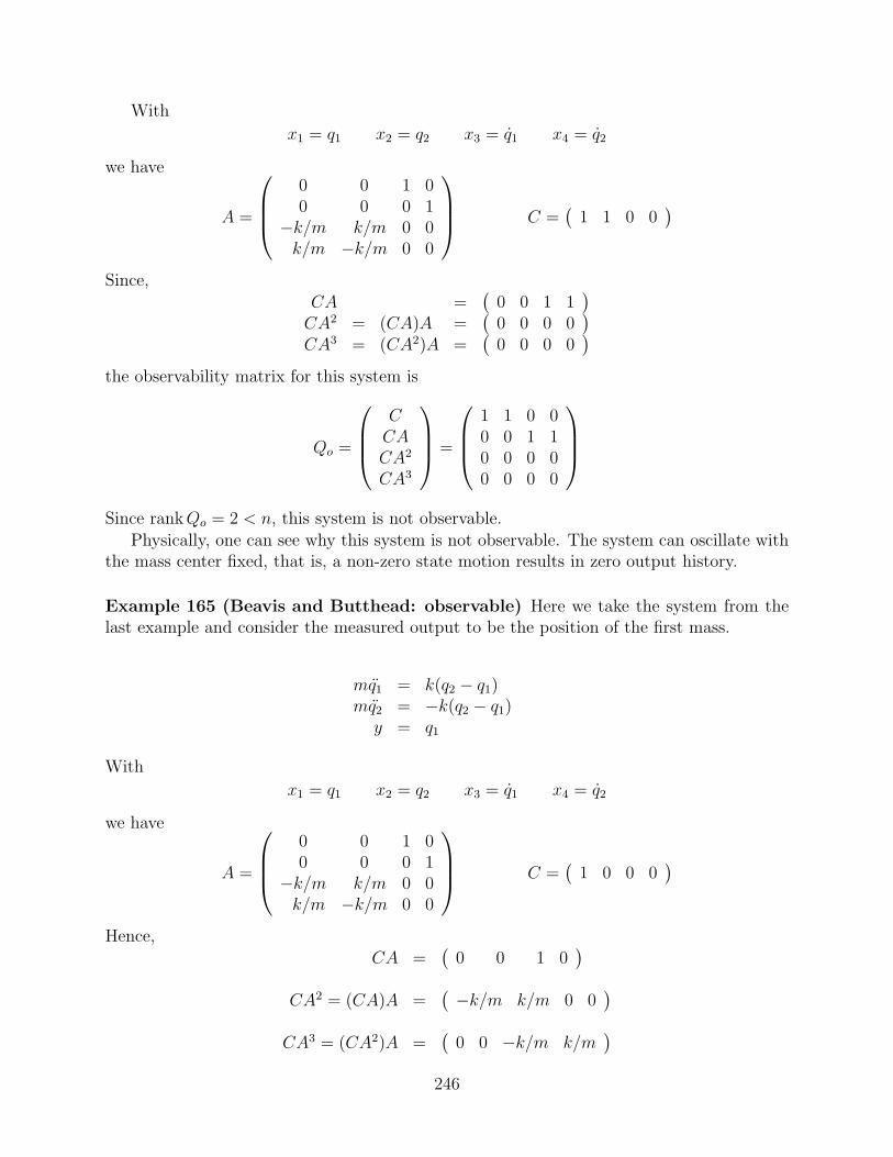
With

x1 = q1 x2 = q2 x3 = q1 x4 = q2

we have

A =

0 0 1 00 0 0 1

−k/m k/m 0 0k/m −k/m 0 0

C =

(1 1 0 0

)

Since,CA =

(0 0 1 1

)CA2 = (CA)A =

(0 0 0 0

)CA3 = (CA2)A =

(0 0 0 0

)

the observability matrix for this system is

Qo =

CCACA2

CA3

=

1 1 0 00 0 1 10 0 0 00 0 0 0

Since rankQo = 2 < n, this system is not observable.Physically, one can see why this system is not observable. The system can oscillate with

the mass center fixed, that is, a non-zero state motion results in zero output history.

Example 165 (Beavis and Butthead: observable) Here we take the system from thelast example and consider the measured output to be the position of the first mass.

mq1 = k(q2 − q1)mq2 = −k(q2 − q1)

y = q1

With

x1 = q1 x2 = q2 x3 = q1 x4 = q2

we have

A =

0 0 1 00 0 0 1

−k/m k/m 0 0k/m −k/m 0 0

C =

(1 0 0 0

)

Hence,CA =

(0 0 1 0

)

CA2 = (CA)A =( −k/m k/m 0 0

)

CA3 = (CA2)A =(

0 0 −k/m k/m)

246

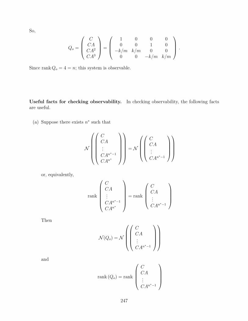
So,

Qo =

CCACA2

CA3

=

1 0 0 00 0 1 0

−k/m k/m 0 00 0 −k/m k/m

.

Since rankQo = 4 = n; this system is observable.

Useful facts for checking observability. In checking observability, the following factsare useful.

(a) Suppose there exists n∗ such that

N

CCA...CAn∗−1

CAn∗

= N

CCA...CAn∗−1

or, equivalently,

rank

CCA...CAn∗−1

CAn∗

= rank

CCA...CAn∗−1

Then

N (Qo) = N

CCA...CAn∗−1

and

rank (Qo) = rank

CCA...CAn∗−1

247

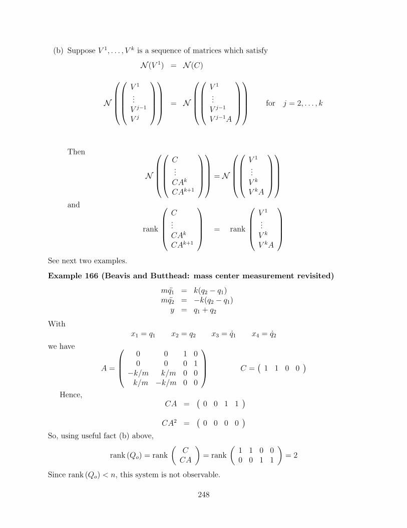
(b) Suppose V 1, . . . , V k is a sequence of matrices which satisfy

N (V 1) = N (C)

N

V 1

...V j−1

V j

= N

V 1

...V j−1

V j−1A

for j = 2, . . . , k

Then

N

C...CAk

CAk+1

= N

V 1

...V k

V kA

and

rank

C...CAk

CAk+1

= rank

V 1

...V k

V kA

See next two examples.

Example 166 (Beavis and Butthead: mass center measurement revisited)

mq1 = k(q2 − q1)mq2 = −k(q2 − q1)

y = q1 + q2

Withx1 = q1 x2 = q2 x3 = q1 x4 = q2

we have

A =

0 0 1 00 0 0 1

−k/m k/m 0 0k/m −k/m 0 0

C =

(1 1 0 0

)

Hence,CA =

(0 0 1 1

)

CA2 =(

0 0 0 0)

So, using useful fact (b) above,

rank (Qo) = rank

(C

CA

)= rank

(1 1 0 00 0 1 1

)= 2

Since rank (Qo) < n, this system is not observable.

248

Example 167 (Beavis and Butthead: observable)

mq1 = k(q2 − q1)mq2 = −k(q2 − q1)

y = q1

With

x1 = q1 x2 = q2 x3 = q1 x4 = q2

we have

A =

0 0 1 00 0 0 1

−k/m k/m 0 0k/m −k/m 0 0

C =

(1 0 0 0

)

Hence,

CA =(

0 0 1 0)

CA2 =( −k/m k/m 0 0

)

So,

rank

CCACA2

= rank

1 0 0 00 0 1 00 1 0 0

and

rank (Qo) = rank

CCACA2

CA3

= rank

1 0 0 00 0 1 00 1 0 00 0 0 1

= 4

Since rankQo = n; this system is observable.

Example 168 State feedback can destroy observability.

A =

(0 10 0

)C =

(1 0

)

(C, A) is observable. Consider

BK =

(0 10 0

)

Then

A + BK = 0

and (C, A + BK) is unobservable.

249

13.3 Development of main result

To develop the main result presented in the last section, we first demonstrate the followingresult:

System (13.1) is observable over an interval [0, T ] if and only if the uncontrolled system(u(t) ≡ 0)

x = Axy = Cx

(13.2)

has the property that the zero state is the only initial state which results in an output historywhich is identically zero; that is, it has the following property:

y(t) = 0 for 0 ≤ t ≤ T implies x(0) = 0

To see that the above property is necessary for observability, simply note that the zeroinitial state produces a zero output history; hence if some nonzero initial state x0 producesa zero output history, then there are two different initial states producing the same outputhistory and the system is not observable.

To see that the above property is sufficient, consider any input history u(·) and supposeya(·) and yb(·) are two output histories due to initial states xa

0 and xb0, repectively, and ya(·) =

yb(·). Let xa(·) and xb(·) be the state histories corresponding the xa0 and xb

0, respectively,that is,

xa = Axa + Bu , xa(0) = xa0

ya = Cxa + Du

and

xb = Axb + Bu , xb(0) = xb0

yb = Cxb + Du

Then, letting

x(t) := xb(t)− xa(t)

y(t) := yb(t)− ya(t)

we obtain

x = Ax , x(0) = xb0 − xa

0

y = Cx

Since y(t) ≡ 0 we must have xb0 − xa

0 = 0; hence xb0 = xa

0. So, system (13.1) is observable.

250


x1 = x2

x2 = 0

If y = x2, the system is unobservable: consider nonzero initial state x0 = [1 0]T ; thecorresponding output history satisfies y(t) ≡ 0. If y = x1, the system is observable. To seethis note that x = [y, y]T . If y(t) ≡ 0 over a nonzero interval, then y(0) = 0 and hence,x(0) = 0.

We have just shown that to investigate the observability of system (13.1), we need onlydetermine the initial states which result in an identically zero output for the system withzero input, that is system (13.2). So, let us look at the consequences of a zero output for theabove system. So, suppose x0 is an initial state which, for some T > 0, results in y(t) = 0for 0 ≤ t ≤ T , that is,

Cx(t) = 0 for 0 ≤ t ≤ T (13.3)

where

x(t) = Ax(t), x(0) = x0 .

Differentiating the equation in (13.3) with respect to t results in

0 = Cx(t) = CAx(t) = 0 for 0 ≤ t ≤ T .

Repeated differentiation of (13.3) yields:

CAkx(t) = 0 for 0 ≤ t ≤ T and k = 0, 1, 2, . . .

Letting t = 0 and using the initial condition x(0) = x0 results in

CAkx0 = 0 for k = 0, 1, 2, . . . . (13.4)

So, we have shown that if an initial state x0 results in a zero output over some nonzerointerval then, (13.4) holds.

Let us now demonstrate the converse, that is, if (13.4) holds, then the resulting outputis zero over any nonzero interval. So, suppose (13.4) holds for some initial state x0. Recallthat x(t) = eAtx0; hence

y(t) = CeAtx0

Since eAt can be expressed as eAt =∑∞

k=0 βk(t)Ak, we have

y(t) = CeAtx0 =∞∑

k=0

β(t)CAkx0 = 0 .

So, we now conclude that an initial state x0 results in a zero output over some nonzerointerval if and only if (13.4) holds. Since, for each k = 0, 1, 2 . . ., the matrix Ak can be

251

expressed as a linear combination of I, A, A2, . . . , An−1, it follows that (13.4) holds if andonly if

CAkx0 = 0 for k = 0, 1, 2, n−1 . (13.5)

Thus an initial state x0 results in a zero output over some nonzero interval if and only if(13.5) holds. Recalling the definition of the observability matrix Qo associated with system(13.1) we obtain the following result:

An initial state x0 results in zero output over some nonzero interval if and only if Qox0 = 0

Hence, system (13.1) is observable if and only if the only vector satisfying Qox0 = 0 isthe zero vector. This immediately leads to the following result on observability. Recall thatthe nullity of a matrix is the dimension of its null space.

For any T > 0, system (13.1) is observable over the interval [0, T ] if and only if thenullity of its observability matrix is zero.

Since the rank and nullity of Qo must sum to n which is the maximum of Qo, we nowobtain main result, that is Theorem 19.

252

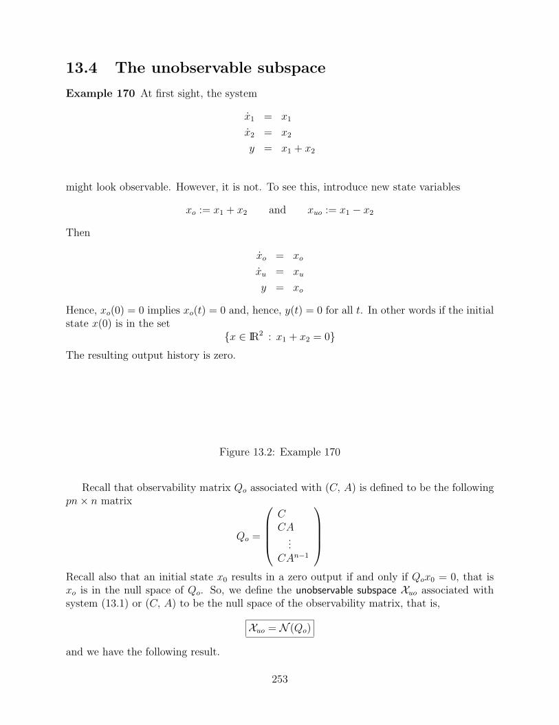
13.4 The unobservable subspace

Example 170 At first sight, the system

x1 = x1

x2 = x2

y = x1 + x2

might look observable. However, it is not. To see this, introduce new state variables

xo := x1 + x2 and xuo := x1 − x2

Then

xo = xo

xu = xu

y = xo

Hence, xo(0) = 0 implies xo(t) = 0 and, hence, y(t) = 0 for all t. In other words if the initialstate x(0) is in the set

x ∈ IR2 : x1 + x2 = 0The resulting output history is zero.

Figure 13.2: Example 170

Recall that observability matrix Qo associated with (C, A) is defined to be the followingpn× n matrix

Qo =

CCA

...CAn−1

Recall also that an initial state x0 results in a zero output if and only if Qox0 = 0, that isxo is in the null space of Qo. So, we define the unobservable subspace Xuo associated withsystem (13.1) or (C, A) to be the null space of the observability matrix, that is,

Xuo = N (Qo)

and we have the following result.

253

Lemma 10 (Unobservable subspace lemma) For any nonzero time interval [0, T ], thefollowing statements are equivalent for system (13.2).

(i) y(t) = 0 for 0 ≤ t ≤ T .

(ii) Qox(0) = 0, or, equivalently, x(0) is in the unobservable subspace Xuo.

Example 171 Recalling the last example we have n = 2 and

A =

(1 00 1

)C =

(1 1

)

Hence,

Qo =

(C

CA

)=

(1 11 1

)

Clearly,Xuo = N (Qo) = N ((

1 1))

= N (C)

HenceN (Qo) = x ∈ IR2 : x1 + x2 = 0

254

13.5 Unobservable modes

Suppose we are interested in the observability of the the input-output system

x = Ax + Bu

y = Cx + Du

Since observability is independent of u, we only need to consider the corresponding zeroinput system:

x = Ax

y = Cx (13.6)

Recall that a mode of this system is a special solution of the form x(t) = eλtv. Such asolution results when x(0) = v and v is an eigenvector of A with eigenvalue λ. We say thateλtv is an unobservable mode of the above system if, the above system has a solution of theform x(t) = eλtv and the corresponding output is zero, that is,

x(t) ≡ eλtv and y(t) ≡ 0

The eigenvalue λ is called an unobservable eigenvalue of the system. We also refer to λ as anunobservable eigenvalue of (C,A).

Clearly, if a system has an unobservable mode then, the system is not observable. Inthe next section, we show that if an LTI system is not observable, then it must have anunobservable mode. Thus:

An LTI system is observable if and only if it has no unobservable modes.

This is illustrated in the following example.

Example 172

x1 = λ1x1 + b1u

x2 = λ2x2 + b2u

y = c1x1 + c2x2 + du

Since

Qo =

(C

CA

)=

(c1 c2

λ1c1 λ2c2

)

This system is observable if and only if

c1 6= 0, c2 6= 0 , λ1 6= λ2

Note that if c1 = 0 then considering u(t) ≡ 0 this system has a solution

x(t) = eλ1t

(10

)

and the corresponding output satisfies

y(t) ≡ 0

255

13.5.1 PBH Test

The next lemma provides a useful characterization of unobservable eigenvalues.

Lemma 11 A complex number λ is an unobservable eigenvalue of the pair (C, A) if andonly if the matrix (

A− λIC

)(13.7)

does not have maximum rank (that is n, where n is the number of columns in A.)

Proof. Recall that λ is an unobservable eigenvalue of (C,A) if the system x = Axhas a non-zero solution of the form x(t) = eλtv which satisfies Cx(t) ≡ 0. We have alreadyseen that the existence of a nonzero solution of the form eλtv is equivalent to v being aneigenvector of A with eigenvalue λ, that is, v 6= 0 and Av = λv; this is equivalent to

(A− λI)v = 0

and v 6= 0. Since x(t) = eλtv and eλt 6= 0, the statement that Cx(t) ≡ 0 is equivalent to

Cv = 0 .

So, we have shown that λ is an unobservable eigenvalue of (C, A) if and only if there is anonzero vector satisfying (

A− λIC

)v = 0 .

The existence of a nonzero v satisfying the above equality is equivalent to saying that thecolumns of the matrix in the equality are linearly dependent, that is, the rank of the matrixis less than the number of its columns. Since the number of columns in the above matrix isless than or equal to the number of its rows, the maximum rank of this matrix equals thenumber of its columns. Hence, λ being an unobservable eigenvalue of (C, A) is equivalent tothe matrix in (13.7) not having maximum rank.

Example 173 Consider a system with

A =

(0 11 0

)B =

(01

)C =

( −1 1)

D = 0 .

Here, the observability matrix is

Qo =

(C

CA

)=

( −1 11 −1

).

Since Qo has zero determinant, this system is not observable. Hence, the system has someunobservable modes. The eigenvalues of A are 1 and −1. To determine the unobservableeigenvalues, we carry out the PBH test:

(A− λI

C

)=

−λ 1

1 −λ−1 1

256

For λ = 1, the above matrix is rank deficient; hence 1 is an unobservable eigenvalue. Forλ = −1, the PBH matrix has maximum rank. Hence, this eigenvalue is observable.

Note that the transfer function for this system is given by

G(s) =s− 1

s2 − 1=

1

s + 1.

So, the unobservable eigenvalue is not a pole of the transfer function. This transfer functionis also the transfer function of the stable system with with A = −1 and B = C = 1 andD = 0.

Since we have already stated that an LTI system is observable if and only if it has nounobservable eigenvalues, we obtain the following corollary to Lemma 11. This new resultprovides another useful test for observability.

Corollary 1 (PBH observability test.) The pair (C, A) is observable if and only if the matrix

(A− λI

C

)

has maximum rank for every eigenvalue λ of A.

Example 174 (Unobservable modes)

A

-2 2 1 2

-1 1 1 2

-3 2 2 2

-1 0 -1 1

B =

2

0

0

2

C

1 0 0 -1

Qo= obsv(A, C)

1 0 0 -1

-1 2 2 1

-7 4 4 7

-9 -2 -2 9

rank(Qo)

2 %System is unobservable

257

eig(A)

1.0000 + 2.0000i

1.0000 - 2.0000i

-1.0000

1.0000

I=eye(4);

rank([A-(-1)*I; C]) %PBH Time

3

rank([A-(1)*I; C])

3

rank([A-(1+2i)*I; C])

4

rank([A-(1-2i)*I; C])

4

So the eigenvalues −1 and +1 are unobservable. The eigenvalues 1 + ı2 and 1 − ı2 are notunobservable.

[num den] = ss2tf(A,B,C,0)

num = 1.0e-013 *

0 -0.0400 0.0933 0.0044 -0.1954

den =

1.0000 -2.0000 4.0000 2.0000 -5.0000

%Actually, the transfer function is ZERO! Why?

Here we observe that unobservable eigenvalues are invariant under a state transformation.To see this consider any state transformation of the form x = T x; then the new PBHobservability matrix is given by

(A− λI

C

)=

(T−1AT − λI

CT

)=

(T−1 00 I

)(A− λI

C

)T

258

Since T is invertible, we see that the new and the old PBH matrices have the same rank.

13.5.2 Existence of unobservable modes*

Here we will show that, if a system is unobservable then, is must have an unobservable mode.So, consider a linear time-invariant input-output system described

x = Ax + Bu (13.8a)

y = Cx + Du (13.8b)

where x(t) is an n-vector, u(t) is an m-vector, and y(t) is a p-vector. Suppose (C, A) is notobservable. In the following section, we show that there is a state transformation x = T x sothat the corresponding transformed system has the following special structure:

xo = Aooxo + Bouxu = Auoxo + Auuxu + Buuy = Coxo + Du

with (xo

xu

)= x .

Also, the pair (Co, Aoo) is observable. Roughly speaking, this transformation splits the stateinto an observable part xo and an unobservable part xu; the subsystem

xo = Aooxo + Bou

y = Coxo + Du

is observable; one can obtain xo from knowledge of the histories of u and y.Notice that, in the transformed system description, there is no connection from the state

xu to the output y. We also note that, when u(t) ≡ 0 and xo(0) = 0 we must have xo(t) ≡ 0.Also,

xu = Auuxu

y = 0

From this it should be clear that, if λ is any eigenvalue of Auu then the transformed system(with zero input) has a solution which satisfies

x(t) = eλtv and y(t) ≡ 0

for some nonzero v, that is λ is an unobservable eigenvalue of the transformed system.Hence, the system

x = Ax , y = Cx

has a nonzero solution x which satisfies

x(t) ≡ eλtv and y(t) ≡ 0

259

Since the matrices A and

A =

(Aoo 0Auo Auu

)

are similar, they have the same characteristic polynomial. Moreover the characteristic poly-nomial of A is given by

det(sI − A) = det(sI − Aoo) det(sI − Auu)

Hence the characteristic polynomial of A is the product of the characteristic polynomials ofAoo and Auu. Thus, the eigenvalues of A are the union of those of Aoo and Auu. Hence, theeigenvalues of Auu are the unobservable eigenvalues of (C,A). The corresponding modes arethe unobservable modes.

Transfer function considerations. Consider the reduced order observable system:

xo = Aooxo + Bou

y = Coxo + Du

One can readily show that the transfer function of this system is exactly the same as thatof the original system, that is,

C(sI − A)−1B + D = Co(sI − Ao)−1Bo + D

13.5.3 A nice transformation*

Consider a LTI input-output system described by

x = Ax + Bu

y = Cx + Du

where x(t) is an n-vector, u(t) is an m-vector, and y(t) is a p-vector. Suppose (C, A) is notobservable; then, its unobservable subspace Xuo is nontrivial. The next lemma states thatXuo is an invariant subspace of A.

Lemma 12 For any n× n matrix A and any p× n matrix, C, the subspace

Xuo = N

CCA...

CAn−1

is an invariant subspace for A.

Proof. Consider any element x of Xuo. It satisfies

CAkx = 0 for k = 0, · · · , n− 1

260

SinceAn = −α0I − α1A− · · · − αn−1A

n−1

we obtainCAnx = 0

from which it follows that

CAk(Ax) = 0 for k = 0, · · · , n− 1

hence Ax is contained in Xuo. Since this holds for every element x of Xuo, it follows that Xuo

is A-invariant.

Transformation. Suppose nu is the dimension of the unobservable subspace Xuo, that is,nu is the nullity of the observability matrix, and let

no := n− nu .

Choose any basistno+1, . . . , tn

for the unobservable subspace, that is, the null space of the observability matrix Qo. Extendit to a basis

t1, . . . , tno , tno+1, . . . , tn

for the whole state space IRn and let

T :=(

t1 t2 . . . tn)

(One could do this by choosing T = V where USV ∗ is a singular value decomposition ofQo). Introduce the state transformation

x = T x

If we let (xo

xu

)= x

where xo is an no-vector and xu is an nu-vector, then

x is in Xuo if and only if xo = 0

The transformed system description is given by

˙x = Ax + Bu

y = Cx + Du

whereA = T−1AT B = T−1B C = CT

261

Since Xuo is an invariant subspace of A, the matrix A has the following structure:

A =

(Aoo 0Auo Auu

)

where Aoo is no× no. Since the vectors tno+1, . . . , tn are in the null space of C, the matrix Chas the following structure

C =(

Co 0)

where Co is p× no. If we partition B as

B =

(Bo

Bu

)

where Bo is no ×m. then the transformed system is described by

xo = Aooxo +Bouxu = Auoxo + Auuxu +Buuy = Coxo +Du

• The pair (Co, Aoo) is observable.

Example 175 (Unobservable modes)

A

-2 2 1 2

-1 1 1 2

-3 2 2 2

-1 0 -1 1

C

1 0 0 -1

Qo= obsv(A, C)

1 0 0 -1

-1 2 2 1

-7 4 4 7

-9 -2 -2 9

rank(Qo)

2 %System is unobservable

eig(A)

1.0000 + 2.0000i

262

1.0000 - 2.0000i

-1.0000

1.0000

I=eye(4);

rank([A-(-1)*I; C]) %PBH Time

3

rank([A-(1)*I; C])

3

rank([A-(1+2i)*I; C])

4

rank([A-(1-2i)*I; C])

4

So the eigenvalues −1 and +1 are unobservable. The eigenvalues 1 + ı2 and 1 − ı2 are notunobservable.

rref(Qo)

1 0 0 -1

0 1 1 0

0 0 0 0

0 0 0 0

N=[1 0 0 1; 0 1 -1 0]’ %Basis for unobservable subspace

1 0

0 1

0 -1

1 0

Qo*N

0 0 %Just checking!

0 0

0 0

0 0

rref([N I])

1 0 0 0 0 1

0 1 0 0 -1 0

0 0 1 0 0 -1

263

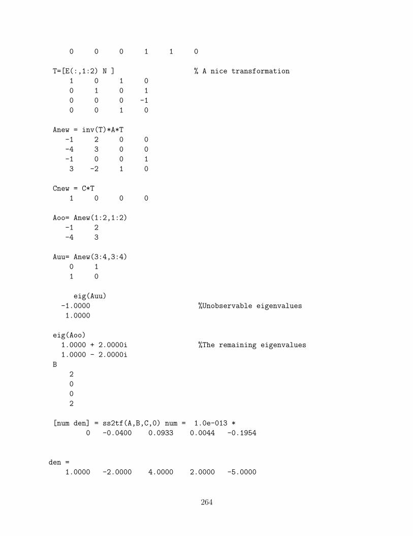
0 0 0 1 1 0

T=[E(:,1:2) N ] % A nice transformation

1 0 1 0

0 1 0 1

0 0 0 -1

0 0 1 0

Anew = inv(T)*A*T

-1 2 0 0

-4 3 0 0

-1 0 0 1

3 -2 1 0

Cnew = C*T

1 0 0 0

Aoo= Anew(1:2,1:2)

-1 2

-4 3

Auu= Anew(3:4,3:4)

0 1

1 0

eig(Auu)

-1.0000 %Unobservable eigenvalues

1.0000

eig(Aoo)

1.0000 + 2.0000i %The remaining eigenvalues

1.0000 - 2.0000i

B

2

0

0

2

[num den] = ss2tf(A,B,C,0) num = 1.0e-013 *

0 -0.0400 0.0933 0.0044 -0.1954

den =

1.0000 -2.0000 4.0000 2.0000 -5.0000

264

%Actually, the transfer function is ZERO! Why?

13.6 Observability grammians*

For each T > 0, we define the finite time observability grammian associated with (C, A):

Wo(T ) =

∫ T

0

eA∗tC∗CeAt dt

To obtain an interpretation of Wo(T ), consider the output y due to zero input and anyinitial state x0, that is,

x = Ax x(0) = x0

y = Cx

Then y(t) = CeAtx0, and

∫ T

0

||y(t)||2 dt =

∫ T

0

||CeAtx0||2 dt =

∫ T

0

(CeAtx0

)∗ (CeAtx0

)dt

=

∫ T

0

x∗0eA∗tC∗CeAtx0 dt = x∗0

(∫ T

0

eA∗tC∗CeAt dt

)x0

= x∗0Wo(T )x0 ;

thus ∫ T

0

||y(t)||2 dt = x∗0Wo(T )x0 .

Remark 6 Note that Wo(T ) is the solution at t = T to the following initial value problem:

Wo = WoA + A∗Wo + C∗C and Wo(0) = 0

Proof. With s = t− τ , we have τ = t− s and

Wc(t) =

∫ t

0

eAτC∗CeA∗τ dτ =

∫ t

0

eA(t−s)C∗CeA∗(t−s) ds

Hence, Wc(0) = 0 and

Wc = AWc + WcA∗ + C∗C

Lemma 13 For each T > 0, the matrices Wo(T ) and Qo have the same null space.

265

Proof. We need to show that N (Qo) = N (Wo(T )). Since

Qo =

CCA...

CA(n−1)

it follows that x is in N (Qo) if and only if

CAkx = 0 for k = 0, 1, . . . , n−1 (13.9)

We first show that N (Qo) ⊂ N (Wo(T )): Consider any x in N (Qo). Then (13.9) holds.Recalling the application of the Cayley-Hamilton theorem to functions of a matrix, it followsthat for 0 ≤ t ≤ T , there are scalars β0(t), . . . , βn−1(t) such that

eAt =n−1∑i=0

βi(t)Ai

Hence,

CeAtx =n−1∑i=0

βi(t)CAix = 0

and

Wo(T )x =

∫ T

0

eA∗tC∗CeAt dt x

=

∫ T

0

eA∗tC∗CeAtx dt

= 0

that is, x is in N (Wo(T )). Since the above holds for any x ∈ N (Qo), we must have N (Qo) ⊂N (Wo(T )).

We now show that N (Wo(T )) ⊂ N (Qo) and hence N (Qo) = N (Wo(T )). To this end,consider any x in N (Wo(T )). Then,

0 = x∗Wo(T )x

= x∗(∫ T

0

eA∗tC∗CeAt dt

)x

=

∫ T

0

x∗eA∗tC∗CeAtx dt

=

∫ T

0

(CeAtx

)∗ (CeAtx

)dt

=

∫ T

0

||CeAtx||2 dt .

266

Since the last integrand is non-negative for all t and the integral is zero, the integrand mustbe zero for all t, that is,

CeAtx ≡ 0 .

If a function is zero for all t, all its derivatives must be zero for all t; hence

CAkeAtx ≡ 0 for k = 0, 1, . . . , n−1 .

Considering t = 0 yields

CAkx = 0 for k = 0, 1, . . . , n−1 ,

that is, x is in N (Qo). Since the above holds for any x in N (Wo(T )), we must haveN (Wo(T )) ⊂ N (Qo).


x1 = x2

x2 = 0

Here

A =

(0 10 0

)eAt =

(1 t0 1

)

(a) (Position measurement.) y = x1. Here

C =(

1 0)

Hence,

Wo(T ) =

∫ T

0

eA∗tC∗CeAt dt =

(T T 2/2

T 2/2 T 3/3

)

and Wo(T ) and Qo have the same null space; that is, 0.(b) (Velocity measurement.) y = x2. Here

C =(

0 1)

Hence,

Wo(T ) =

∫ T

0

eA∗tC∗CeAt dt =

(0 00 T

)

and Wo(T ) and Qo have the same null space.

The above lemma has the following consequence.

The pair (C,A) is observable if and only if for every T > 0 the corresponding observabilitygrammian is invertible.

267

Computation of initial state. One reason for introducing the observability grammianis as follows: Suppose (C,A) is observable; then from the above lemma, Wo(T ) is invertible.The output for

x = Ax + Bu x(0) = x0

y = Cx + Du

is given by

y(t) = CeAtx0 +

∫ t

0

CeA(t−τ)Bu(τ) dτ + Du(t)

Letting

y(t) = y(t)−∫ t

0

CeA(t−τ)Bu(τ) dτ −Du(t)

we have y(t) = CeAtx0 and

∫ T

0

eA∗tC∗y(t) dt =

∫ T

0

eA∗tC∗CeAtx0 dt

= Wo(T )x0 .

Since Wo(T ) is invertible, we obtain the following explicit expression for the initial state interms of the input and output histories:

x0 = Wo(T )−1∫ T

0eA∗tC∗y(t) dt

The above expression explicitly shows us that if a system is observable, we can obtain theinitial state from measurements of the input and output over any time interval. However,this formula is not usually used to obtain the state. One usually uses asymptotic observersor state estimators to asymptotically obtain the state; these are covered in a later chapter.

13.6.1 Infinite time observability grammian

Suppose A is asymptotically stable, that is, all its eigenvalues have negative real parts, andconsider the linear matrix equation

WoA + A∗Wo + C∗C = 0

This is a Lyapunov equation of the form PA + A∗P + Q = 0 with Q = C∗C. Since A isasymptotically stable the above equation has a unique solution for Wo and this solution isgiven by

Wo =

∫ ∞

0

eA∗tC∗CeAtdt

We call this matrix the (infinite-time) observability grammian associated with (C, A). Onemay show that Wo and the observability matrix Qo have the same null-space. Since Wo is asymmetric positive definite matrix, it follows that the null space of Wo is 0 if and only ifWo is positive definite. Hence, we have the following result.

268

Lemma 14 Suppose all the eigenvalues of A have negative real parts. Then (C, A) is ob-servable if and only if Wo is positive definite.

Note that if y is the output of the system

x = Ax

y = Cx

with initial condition x(0) = x0 then

∫ ∞

0

‖y(t)‖2 dt = x∗0W0x0

This follows from y(t) = CeAtx0 and

∫ ∞

0

‖y(t)‖2 dt =

∫ ∞

0

y(t)∗y(t) dt

=

∫ ∞

0

(CeAtx0)∗CeAtx0 dt

= x∗0

∫ ∞

0

eA∗tC∗CeAt dt x0

= x∗0W0x0 .

269

13.7 Discrete time

Consider the discrete-time system described by

x(k + 1) = Ax(k) + Bu(k)y(k) = Cx(k) + Du(k)

(13.10)

where k ∈ ZZ is time, x(k) ∈ IRn is the state, u(k) ∈ IRm is the input, and y(k) ∈ IRp is themeasured output.

Consider any fixed time N > 0. The basic observability problem is as follows. Sup-pose we have knowledge of the input sequence u(0), u(1), · · · , u(N) and output sequence y(0), y(1), · · · , y(N) over the interval [0, N ]. Can we uniquely determine the initial state

x0 = x(0)

If we can do this for input histories and all initial states we say the system is observable.

DEFN. System (13.10) is observable over the interval [0, N ] if the following holds for eachinput history u(·). Suppose ya(·) and yb(·) are any two output histories of system (13.1) dueto initial states xa

0 and xb0, respectively, and ya(k) = yb(k) for 0 ≤ k ≤ N ; then xa

0 = xb0.

• Our first observation is that system (13.10) is observable over [0, N ] if and only if thesystem

x(k + 1) = Ax(k)y(k) = Cx(k)

(13.11)

has the property that the zero state is the only initial state resulting in an output historywhich is identically zero; that is, it has the the following property:

y(k) = 0 for 0 ≤ k ≤ N =⇒ x(0) = 0

13.7.1 Main observability result

Theorem 20 (Main observability theorem) For each N ≥ n− 1 , system (13.10) isobservable over [0, N ] if and only if

rank

CCA...CAn−1

= n

Proof. The proof can be obtained by showing that, for system (13.11) with x0 = x(0),

y(0)y(1)

...y(n−1)

=

Cx0

CAx0...CAn−1x0

= Q0x0

Also use Cayley Hamilton.

270

13.8 Exercises

Exercise 109 Determine whether or not each of the following systems are observable.

x1 = −x1

x2 = x2 + uy = x1 + x2

x1 = −x1

x2 = x2 + uy = x2

x1 = x1

x2 = x2 + uy = x1 + x2

x1 = x2

x2 = 4x1 + uy = −2x1 + x2

Exercise 110 Consider the system with input u, output y, and state variables x1, x2 de-scribed by

x1 = −3x1 + 2x2 + u

x2 = −4x1 + 3x2 + 2u

y = −2x1 + x2

(a) Is this system observable?(b) If the system is unobservable, determine the unobservable eigenvalues.

Exercise 111 Determine (by hand) whether or not the following system is observable.

x1 = 5x1 − x2 − 2x3

x2 = x1 + 3x2 − 2x3

x3 = −x1 − x2 + 4x3

y1 = x1 + x2

y2 = x2 + x3

If the system is unobservable, compute the unobservable eigenvalues.

Exercise 112 Determine the unobservable eigenvalues for each of the systems of Exercise109.

Exercise 113 For each system in Exercise 109 which is not observable, obtain a reducedorder system which is observable and has the same transfer function as the original system.

Exercise 114 (Damped linear oscillator.) Recall

x1 = x2

x2 = −(k/m) x1 − (d/m) x2

Show the following:

(a) (Position measurement.) If y = x1, we have observability.

(b) (Velocity measurement.) If y = x2, we have observability if and only if k 6= 0.

(c) (Acceleration measurement.) If y = x2, we have observability if and only if k 6= 0.

271

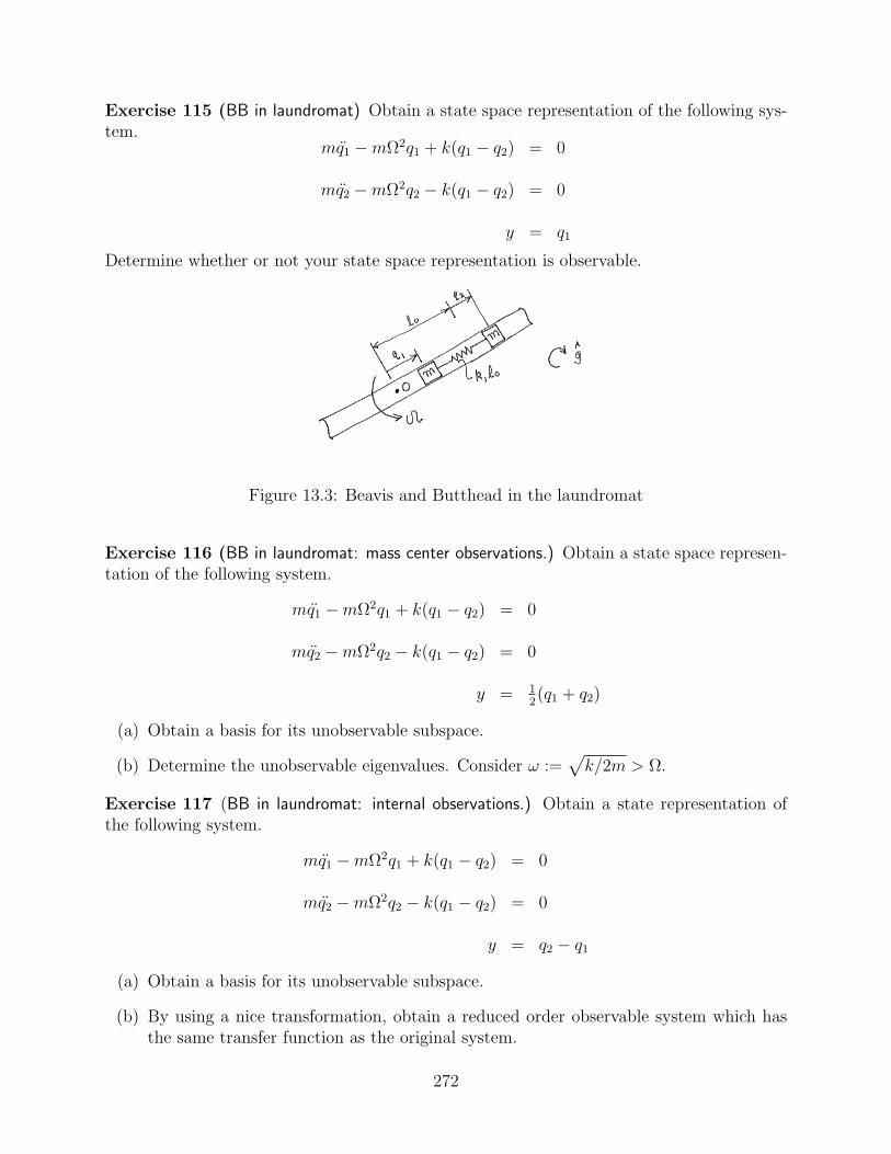
Exercise 115 (BB in laundromat) Obtain a state space representation of the following sys-tem.

mq1 −mΩ2q1 + k(q1 − q2) = 0

mq2 −mΩ2q2 − k(q1 − q2) = 0

y = q1

Determine whether or not your state space representation is observable.

Figure 13.3: Beavis and Butthead in the laundromat

Exercise 116 (BB in laundromat: mass center observations.) Obtain a state space represen-tation of the following system.

mq1 −mΩ2q1 + k(q1 − q2) = 0

mq2 −mΩ2q2 − k(q1 − q2) = 0

y = 12(q1 + q2)

(a) Obtain a basis for its unobservable subspace.

(b) Determine the unobservable eigenvalues. Consider ω :=√

k/2m > Ω.

Exercise 117 (BB in laundromat: internal observations.) Obtain a state representation ofthe following system.

mq1 −mΩ2q1 + k(q1 − q2) = 0

mq2 −mΩ2q2 − k(q1 − q2) = 0

y = q2 − q1

(a) Obtain a basis for its unobservable subspace.

(b) By using a nice transformation, obtain a reduced order observable system which hasthe same transfer function as the original system.

272

(c) Determine the unobservable eigenvalues. Consider ω :=√

k/2m > Ω.


x1 = λ1x1 + b1u

x2 = λ2x2 + b2u...

xn = λnxn + bnu

y = c1x1 + c2x2 + · · ·+ cnxn

where all quantities are scalar. Obtain conditions on the numbers λ1, · · · , λn and c1, · · · , cn

which are necessary and sufficient for the observability of this system.

Exercise 119 Compute the observability grammian for the damped linear oscillator withposition measurement and d, k > 0.

Exercise 120 Carry out the following for linearizations L1-L8 of the two pendulum cartsystem.

(a) Determine which linearizations are observable?

(b) Compute the singular values of the observability matrix.

(b) Determine the unobservable eigenvalues for the unobservable linearizations.

273

Chapter 14

Controllability

14.1 Controllability

Consider a system in which x(t) is the system state at time t and u(t) is the control input attime t. Consider now any non-trivial time interval [0, T ]; by non-trivial we mean that T > 0.We say that the system is controllable over the interval if it can be ‘driven’ from any onestate to any other state over the time interval by appropriate choice of control input overthe interval. A formal definition follows the next two examples.

Example 177 (Two unattached masses)

x1 = u

x2 = 0

Since the behavior of x2 is completely unaffected by the control input u, this system is clearlyuncontrollable over any time interval.

Example 178 (Integrator) Consider the scalar system described by

x = u

Consider any initial state x0 and any desired final state xf . For any any T > 0, consider theconstant input:

u(t) = (xf − x0)/T for 0 ≤ t ≤ T

Then the state trajectory x(·) of this system with x(0) = x0 satisfies x(T ) = xf . We considerthis system to be controllable over any time interval [0, T ].

DEFN.[Controllability] A system is controllable over a non-trivial time interval [0, T ] if, forevery pair of states x0 and xf , there is a continuous control function u(·) defined on theinterval such that the solution x(·) of the system with x(0) = x0 satisfies x(T ) = xf .

Note that the definition says nothing about keeping the state at xf after T .

275

Figure 14.1: Controllability

14.2 Main controllability result

The concept of controllability also applies to linear and nonlinear systems. However, we areconcerned here with linear time-invariant systems described by

x = Ax + Bu (14.1)

where the n-vector x(t) is the system state at time t and the m-vector u(t) is the controlinput at time t. In this section, we introduce a simple algebraic condition which is necessaryand sufficient for the controllability of a linear time invariant system over any time interval.This condition involves the controllability matrix Qc associated with the above system or thepair (A, B). This matrix is defined to be the following n× nm partitioned matrix:

Qc =(

B AB · · · An−1B)

(14.2)

Theorem 21 (Main controllability result) For any T > 0, system (14.1) is controllableover the interval [0, T ] if and only if its controllability has maximum rank, that is,

rank(

B AB · · · An−1B)

= n

Proof. A proof is given at the end of Section 14.3.

An immediate consequence of the above theorem is that controllability does not dependon the interval [0, T ]. So, from now on we drop reference to the interval. Since controllabilityonly depends on the matrix pair (A,B), we say that this pair is controllable if system (14.1)is controllable.

For scalar input (m = 1) systems, the controllability matrix is a square matrix; hence ithas maximum rank if and only if its determinant is nonzero. So, the above theorem has thefollowing corollary.

Corollary 2 A scalar input system of the form (14.1) is controllable if and only if its con-trollability matrix has non-zero determinant.

276

Example 179 (Two unattached masses.) This is a scalar input system with

A =

(0 00 0

)and B =

(10

).

Hence,

Qc =(

B AB)

=

(1 00 0

)

Clearly Qc has zero determinant, hence this system is not controllable.

Example 180

x1 = x3 + u1

x2 = x3 + u1

x3 = u2

Since there is a control input entering every state equation, this system looks controllable.Is it?

Here n = 3 and

A =

0 0 10 0 10 0 0

B =

1 01 00 1

So,

Qc =(

B AB A2B)

=

1 0 0 1 0 01 0 0 1 0 00 1 0 0 0 0

and

rank (Qc) = rank

1 01 00 1

= 2

Since rankQc = 2, we have rank Qc 6= n; hence this system is not controllable.

MATLAB

>> help ctrb

CTRB Form controllability matrix.

CTRB(A,B) returns the controllability matrix

Co = [B AB A^2B ...]

>> A=[0 0 1; 0 0 1; 0 0 0];

>> B=[1 0; 1 0; 0 1];

>> ctrb(A,B)

ans =

1 0 0 1 0 0

1 0 0 1 0 0

0 1 0 0 0 0

277

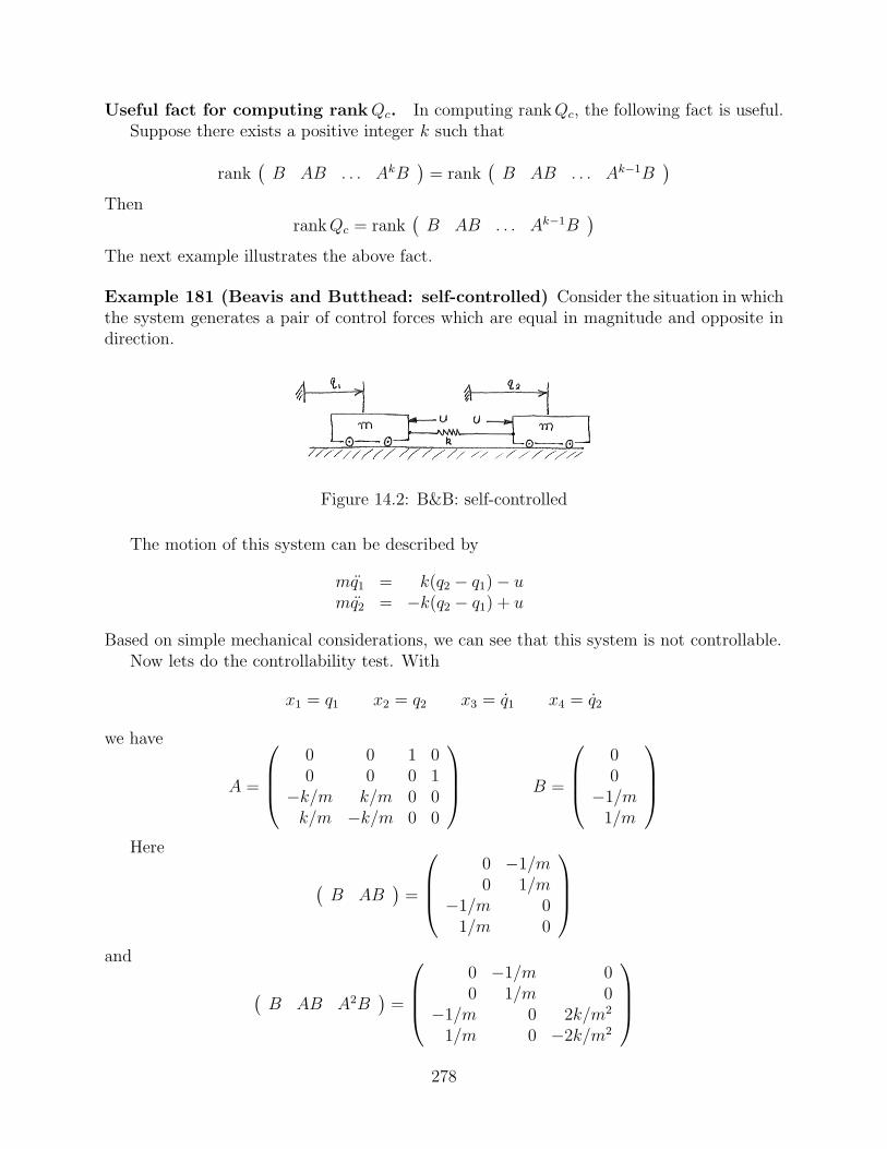
Useful fact for computing rank Qc. In computing rank Qc, the following fact is useful.Suppose there exists a positive integer k such that

rank(

B AB . . . AkB)

= rank(

B AB . . . Ak−1B)

ThenrankQc = rank

(B AB . . . Ak−1B

)

The next example illustrates the above fact.

Example 181 (Beavis and Butthead: self-controlled) Consider the situation in whichthe system generates a pair of control forces which are equal in magnitude and opposite indirection.

Figure 14.2: B&B: self-controlled

The motion of this system can be described by

mq1 = k(q2 − q1)− umq2 = −k(q2 − q1) + u

Based on simple mechanical considerations, we can see that this system is not controllable.Now lets do the controllability test. With

x1 = q1 x2 = q2 x3 = q1 x4 = q2

we have

A =

0 0 1 00 0 0 1

−k/m k/m 0 0k/m −k/m 0 0

B =

00

−1/m1/m

Here

(B AB

)=

0 −1/m0 1/m

−1/m 01/m 0

and

(B AB A2B

)=

0 −1/m 00 1/m 0

−1/m 0 2k/m2

1/m 0 −2k/m2

278

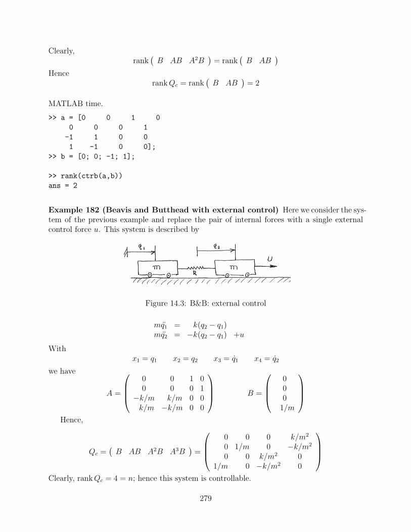
Clearly,rank

(B AB A2B

)= rank

(B AB

)

Hencerank Qc = rank

(B AB

)= 2

MATLAB time.

>> a = [0 0 1 0

0 0 0 1

-1 1 0 0

1 -1 0 0];

>> b = [0; 0; -1; 1];

>> rank(ctrb(a,b))

ans = 2

Example 182 (Beavis and Butthead with external control) Here we consider the sys-tem of the previous example and replace the pair of internal forces with a single externalcontrol force u. This system is described by

Figure 14.3: B&B: external control

mq1 = k(q2 − q1)mq2 = −k(q2 − q1) +u

Withx1 = q1 x2 = q2 x3 = q1 x4 = q2

we have

A =

0 0 1 00 0 0 1

−k/m k/m 0 0k/m −k/m 0 0

B =

000

1/m

Hence,

Qc =(

B AB A2B A3B)

=

0 0 0 k/m2

0 1/m 0 −k/m2

0 0 k/m2 01/m 0 −k/m2 0

Clearly, rankQc = 4 = n; hence this system is controllable.

279

Exercise 121 Suppose A is n× n, B is n×m, T is n× n and nonsingular and let

A = T−1AT B = T−1B

Then (A,B) is controllable if and only if (A, B) is controllable.

14.3 The controllable subspace

Let us now consider the situation when the system x = Ax + Bu is not controllable.

Example 183 At first sight the system

x1 = x1 + u

x2 = x2 + u

might look controllable. However, it is not. To see this, consider the following change ofstate variables:

xc = x1 + x2 and xu = x1 − x2

These variables satisfy

xc = xc + 2u

xu = xu

Hence, xu(0) = 0 implies xu(t) = 0 for all t. In other words if the initial x(0) is in the set

(x1, x2) ∈ IR2 : x1 − x2 = 0

then, regardless of the control input, the state will always stay in this set; it cannot leavethis set. So, the system is not controllable.

Figure 14.4: Controllable subspace in Example 183

280

Recall that the controllability matrix associated with the pair (A, B) is defined to be thefollowing n× nm matrix

Qc =(

B AB . . . An−1B)

The controllable subspace is defined as the range of the controllability matrix, that is,

R(Qc)

So, according to the Main Controllability Theorem (Theorem 21), the system x = Ax+Buis controllable if and only if its controllable subspace is the whole state space. It should beclear that a vector x is in the controllable subspace associated with (A, B) if and only if itcan be expressed as

x =n−1∑i=0

AiBνi

where ν0, . . . , νn−1 are m-vectors.The following lemma states that when the state of system (14.1) starts at zero, then

regardless of the control input, the state always stays in the controllable subspace; that is,it cannot leave this subspace.

Lemma 15 If x(0) = 0 then, for every continuous control input function u(·), the solutionx(·) of (14.1) lies in the controllable subspace, that is, x(t) is in the range of Qc for all t ≥ 0.

Proof. For any time t > 0 we have

x(t) =

∫ t

0

eA(t−τ)Bu(τ) dτ

Recalling the application of the Cayley-Hamilton theorem to functions of a matrix, it followsthat for 0 ≤ τ ≤ t, there are scalars β0(τ), . . . , βn−1(τ) such that

eA(t−τ) =n−1∑i=0

βi(τ)Ai

Hence,

eA(t−τ)Bu(τ) =n−1∑i=0

AiBνi(τ) νi(τ) := βi(τ)u(τ)

From this it should be clear that for each τ , the n vector eA(t−τ)Bu(τ) is in R(Qc), the rangeof Qc. From this one obtains that x(t) =

∫ t

0eA(t−τ)Bu(τ) dτ is in R(Qc).

Example 184 For the system of example 183, we have

Qc =(

B AB)

=

(1 11 1

)

281

Clearly,

R(Qc) = R((

11

))= R (B)

If a vector x is in this controllable subspace, then x = c [ 1 1 ]T for some scalar c. This isequivalent to the requirement that x1 − x2 = 0.

Actually, if the state starts at any point in R(Qc) then, regardless of the control input,the state always stays in R(Qc); see next exercise. In other words, the control input cannotdrive the state out of the controllable subspace.

Figure 14.5: Invariance of the controllable subspace

Exercise 122 Prove the following statement. If x(0) is in R(Qc), then for every continuouscontrol input function u(·), the solution of (14.1) satisfies x(t) ∈ R(Qc) for all t ≥ 0.

The next result states that over any time interval, system (14.1) can be driven betweenany two states in the controllable subspace R(Qc) by appropriate choice of control input.

Lemma 16 [Controllable subspace lemma] Consider any pair of states x0, xf in the con-trollable subspace R(Qc). Then for each T > 0, there is a continuous control functionu(·) : [0, T ] → IRm such that the solution x(·) of (14.1) with x(0) = x0 satisfies x(T ) = xf

Proof. A proof is contained in section 14.4.

Example 185

x1 = −x1 + x2 + u

x2 = −x1 + x2 + u

Here,

A =

( −1 1−1 1

)B =

(11

)

Hence

Qc =(

B AB)

=

(1 01 0

)

282

and

R(Qc) = R((

11

))

To illustrate the controllable subspace lemma, introduce new states

xc = x1 xu = −x1 + x2

Then

x = xc

(11

)+ xu

(01

)

and

xc = xu + u

xu = 0

It should be clear that x is in the controllable subspace if and only if xu = 0. In this case xis completely specified by the scalar xc and

xc = u

Recalling example 178, we see that given any xc0, xcf and any T > 0, one can always finda control input which ‘drives’ xc from xc0 to xcf over the interval [0, T ]. Hence, the state xcan be driven between any two points in the controllable subspace.

Proof of main controllability result. First note that rankQc = n if and only ifR(Qc) =IRn, that is, the controllability matrix has rank n if and only if the controllable subspace isthe whole state space. If rank Qc = n, then Lemma 16 implies controllability. If rank Qc < n,then the controllable subspace is not the whole state space and from Lemma 15 any statewhich is not in the controllable subspace cannot be reached from the origin.

283

14.4 Proof of the controllable subspace lemma*

14.4.1 Finite time controllability grammian

Before proving the controllable subspace lemma, we first establish a preliminary lemma. Foreach T > 0, we define the finite time controllability grammian associated with (A,B):

Wc(T ) :=

∫ T

0

eAtBB∗eA∗t dt (14.3)

Note that this matrix is hermitian and positive semi-definite.

Remark 7 Note that Wc(T ) is the solution at t = T of the following initial value problem:

Wc = AWc + WcA∗ + BB∗ and Wc(0) = 0

Proof.

Wc(t) =

∫ t

0

eAτBB∗eA∗τ dτ =

∫ t

0

eA(t−s)BB∗eA∗(t−s) ds

Hence, Wc(0) = 0 andWc = AWc + WcA

∗ + BB∗

Lemma 17 For each T > 0,R(Wc(T )) = R(Qc)

Proof. We will show that N (Q∗c) = N (Wc(T )). From this it will follow that R(Qc) =

R(Wc(T )∗) = R(Wc(T )).Since

Q∗c =

B∗

B∗A∗...

B∗A∗(n−1)

it follows that x is in N (Q∗c) if and only if

B∗A∗kx = 0 for k = 0, 1, . . . , n−1 (14.4)

We first show that N (Q∗c) ⊂ N (Wc(T )): Consider any x ∈ N (Q∗

c). Then (14.4) holds.Recalling the application of the Cayley-Hamilton theorem to functions of a matrix, it followsthat for 0 ≤ t ≤ T , there are scalars β0(t), . . . , βn−1(t) such that

eA∗t =n−1∑i=0

βi(t)A∗i

284

Hence,

B∗eA∗tx =n−1∑i=0

βi(t)B∗A∗ix = 0

and

Wc(T )x =

∫ T

0

eAtBB∗eA∗t dt x

=

∫ T

0

eAtBB∗eA∗tx dt

= 0

that is, x ∈ N (Wc(T )). Since the above holds for any x ∈ N (Q∗c), we must have N (Q∗

c) ⊂N (Wc(T )).

We now show that N (Wc(T )) ⊂ N (Q∗c) and hence N (Q∗

c) = N (Wc(T )): Consider anyx ∈ N (Wc(T )). Then,

0 = x∗Wc(T )x

= x∗(∫ T

0

eAtBB∗eA∗t dt

)x

=

∫ T

0

x∗eAtBB∗eA∗tx dt

=

∫ T

0

(B∗eA∗tx

)∗ (B∗eA∗tx

)dt

=

∫ T

0

||B∗eA∗tx||2 dt

Since the integrand is non-negative for all t and the integral is zero, the integrand must bezero for all t, that is,

B∗eA∗tx ≡ 0

If a function is zero for all t, all its derivatives must be zero for all t; hence

B∗A∗keA∗tx ≡ 0 for k = 0, 1, . . . , n−1

Considering t = 0 yields

B∗A∗kx = 0 for k = 0, 1, . . . , n−1

that is x ∈ N (Q∗c). Since the above holds for any x ∈ N (Wc(T )), we must have N (Wc(T )) ⊂

N (Q∗c).

From our main controllability result and the above lemma, we see that (A,B) is control-lable if and only if , for any T > 0, its finite time controllability grammian Wc(T ) has fullrank. Since Wc(T ) is square, it has full rank if and only if it is invertible. Moreover, sinceWc(T ) is symmetric and positive semidefinite, it has full rank if and only if it is positivedefinite. This yields the following result.

285

Corollary 2 The system x = Ax + Bu is controllable if and only if its controllability gram-mian over any non-trivial interval is positive definite.

14.4.2 Proof of the controllable subspace lemma

Consider any T > 0 and any pair of states x0, xf in R(Qc). The solution of (14.1) at time Tis:

x(T ) = eAT x0 +

∫ T

0

eA(T−τ)Bu(τ) dτ

Hence, a control input drives the state from x0 to xf if and only if

∫ T

0

eA(T−τ)Bu(τ) dτ = z := xf − eAT x0

We first show that

z ∈ R(Qc)

Since x0 ∈ R(Qc),

x0 =n−1∑i=0

AiBνi

hence

eAT x0 =n−1∑i=0

eAT AiBνi

By application of Cayley Hamilton to functions of a matrix

eAT Ai =n−1∑

k=0

βikAk

so,

eAT x0 =n−1∑i=0

n−1∑

k=0

βikAkBνi =

n−1∑

k=0

AkBνk

where νk :=∑n−1

i=0 βikνi. From this it should be clear that eAT x0 is in R(Qc). Since xf is

also in R(Qc) we have z ∈ R(Qc).Since z is in R(Qc), it follows from the previous lemma that z is also in R(Wc(T )). Hence

there exists an n-vector y such that

z = Wc(T )y

Considering the control input

u(τ) = B∗eA∗(T−τ)y

286

we obtain

∫ T

0

eA(T−τ)Bu(τ) dτ =

∫ T

0

eA(T−τ)BB∗eA∗(T−τ)y dτ

=

∫ T

0

eA(T−τ)BB∗eA∗(T−τ) dτ y

=

∫ T

0

eAtBB∗eA∗t dt y

= Wc(T )y

= z

hence, this control input drives the state from x0 to xf .

Remark 8 Suppose (A,B) is controllable. Then rank Wc(T ) = rankQc = n. Hence Wc(T )is invertible and the control which drives x0 to xf over the interval [0, T ] is given by

u(t) = B∗eA∗(T−t)x x = Wc(T )−1(xf − eAT x0)

14.5 Uncontrollable modes

We shall see that if a system is uncontrollable, it has modes which cannot be affected by theinput. To define exactly what we mean by an uncontrollable mode, we need to look at theleft eigenvectors of the system A matrix.

14.5.1 Eigenvectors revisited: left eigenvectors

Suppose that λ is an eigenvalue of a square matrix A. Then an eigenvector correspondingto λ is any nonzero vector satisfying Av = λv. We say that a nonzero vector w is a lefteigenvector of A corresponding to λ if it satisfies

w′A = λw′ (14.5)

To see that left eigenvectors exist, note that the above equation is equivalent to A′w = λw,that is, λ is an eigenvalue of A′ and w is an eigenvector of A′ corresponding to λ. We nowrecall that λ is an eigenvalue of A if and only if λ is an eigenvalue of A′ . Thus, we cansay that λ is an eigenvalue of A if and only if it satisfies (14.5) for some non-zero vectorw. Moreover, we can also say that every eigenvalue λ of A has left eigenvectors and thesevectors are simply the eigenvectors of A′ corresponding to λ.

Consider now any two eigenvectors λ1 and λ2 of A with λ1 6= λ2. Suppose that v1 is aneigenvector for λ1 and w2 is a left eigenvector for λ2. Then

w′2v1 = 0 .

287

To see this, we first use the eigenvector definitions to obtain

Av1 = λ1v1 and w′2A = λ2w

′2 .

Pre-multiplying the first equation by w′2 we obtain that w′

2Av1 = λ1w′2v1. Post-multiplying

the section equation by v1 we obtain that w′2Av1 = λ2w

′2v1. This implies that λ1w

′2v1 =

λ2w′2v1, that is (λ1 − λ2)w

′2v1 = 0. Since λ1 − λ2 6= 0, we must have w′

2v1 = 0.

System significance of left eigenvectors. Consider now a system described by

x = Ax . (14.6)

Recall that λ is an eigenvalue of A if and only if the above system has a solution of the formx(t) = eλtv where v is a nonzero constant vector. When this occurs, the vector v can be anyeigenvector of A corresponding to λ and the above special solution is described as a modeof the system. We now demonstrate the following result:

A scalar λ is an eigenvalue of A if and only if there is a nonzero vector w such that everysolution x(·) of system (14.6) satisfies

w′x(t) = eλtw′x(0) (14.7)

When this occurs, the vector w can be any left eigenvector of A corresponding to λ.

In particular, if x(0) = w/||w||2 then, w′x(t) = eλt. If w′x(0) = 0 then w′x(t) = 0 for allt.

To gain further insight into the above result, introduce the scalar variable ξ(t) = w′x(t).Then ξ(0) = w′x(0) and (14.7) is equivalent to

ξ(t) = eλtξ(0) ,

that is, the behavior of ξ is governed by

ξ = λξ .

To demonstrate the above result, we first suppose that λ is an eigenvalue of A. Then thereis a nonzero vector w such that (14.5) holds; also w is a left eigenvector of A correspondingto λ. Consider now any solution x(·) of system (14.6). Since it satisfies x = Ax, it followsfrom (14.5) that

d(w′x)

dt= w′x = w′Ax = λ(w′x)

It now follows that (14.7) holds for all t.To demonstrate the converse, suppose that there is a nonzero vector w so that (14.7)

holds for every solution x(·). This implies that

w′Ax(t) = w′x(t) =d(w′x)

dt= λeλtw′x(0) = λw′x(t) ;

hence,w′(A− λI)x(t) = 0 .

Since the above holds for any x(t), we must have w′(A − λI) = 0. Thus, w′A = λw′. Thisimplies that λ is an eigenvalue of A with left eigenvector w.

288

14.5.2 Uncontrollable eigenvalues and modes

Consider now a system with input u described by

x = Ax + Bu (14.8)

We say that λ is an uncontrollable eigenvalue of this system or λ is an uncontrollable eigen-value of (A,B) if there is a nonzero vector w such that for every input u(·), every solutionx(·) of the system satisfies

w′x(t) = eλtw′x(0) (14.9)

To gain further insight into the above concept, introduce the scalar variable ξ(t) = w′x(t).Then, as we have shown above, (14.9) is equivalent to the statement that the behavior of ξis governed by

ξ = λξ .

Thus the behavior of ξ is completely unaffected by the input u. So, the mode eλt is completelyunaffected by the input u. We say that this is an uncontrollable mode.

When system (14.8) has an uncontrollable mode, then the system is not controllable. Tosee this choose any initial state x(0) = x0 such that w′x0 6= 0. Then, regardless of the controlinput, we have w′x(t) = eλtw′x0 6= 0 for all t. Hence, regardless of the control input, x(t) 6= 0for all t. This means that over any time interval [0, T ] we cannot obtain a control historywhich drives the system from x0 to 0. Hence the system is not controllable. In Section14.5.3, we demonstrate the following result.

If a system is not controllable then, it must have some uncontrollable modes.

14.5.3 Existence of uncontrollable modes*

In this section, we show that if a LTI system is not controllable, then it has uncontrollablemodes. Consider a linear time-invariant input-output system described

x = Ax + Bu

y = Cx + Du (14.10)

where x(t) is an n-vector, u(t) is an m-vector, and y(t) is a p-vector. Suppose (A,B) isnot controllable; then, its controllable subspace Xc is not equal to the whole state space.In the following section, we show that there is a state transformation x = T x so that thecorresponding transformed system is described by

xc = Accxc + Acuxu + Bcu

xu = Auuxu

y = Ccxc + Cuxu + Du (14.11)

with (xc

xu

)= x .

289

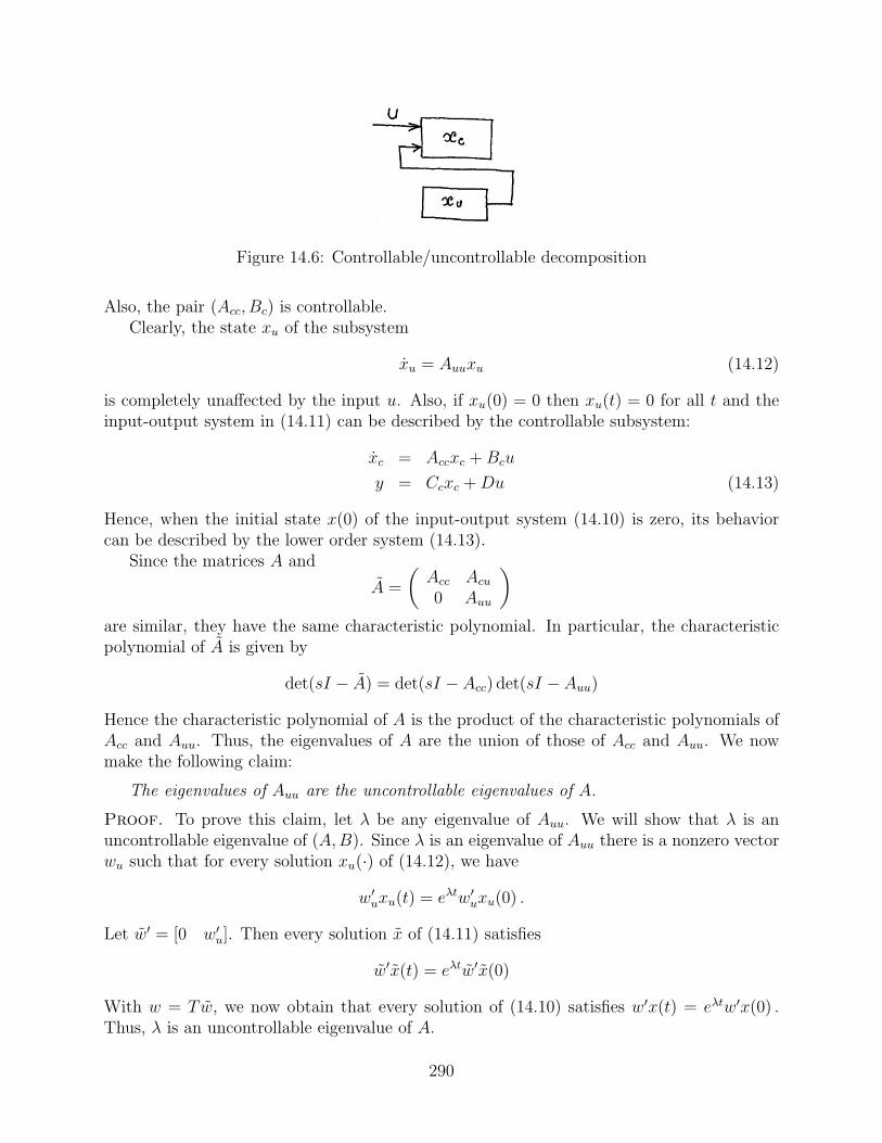
Figure 14.6: Controllable/uncontrollable decomposition

Also, the pair (Acc, Bc) is controllable.Clearly, the state xu of the subsystem

xu = Auuxu (14.12)

is completely unaffected by the input u. Also, if xu(0) = 0 then xu(t) = 0 for all t and theinput-output system in (14.11) can be described by the controllable subsystem:

xc = Accxc + Bcu

y = Ccxc + Du (14.13)

Hence, when the initial state x(0) of the input-output system (14.10) is zero, its behaviorcan be described by the lower order system (14.13).

Since the matrices A and

A =

(Acc Acu

0 Auu

)

are similar, they have the same characteristic polynomial. In particular, the characteristicpolynomial of A is given by

det(sI − A) = det(sI − Acc) det(sI − Auu)

Hence the characteristic polynomial of A is the product of the characteristic polynomials ofAcc and Auu. Thus, the eigenvalues of A are the union of those of Acc and Auu. We nowmake the following claim:

The eigenvalues of Auu are the uncontrollable eigenvalues of A.

Proof. To prove this claim, let λ be any eigenvalue of Auu. We will show that λ is anuncontrollable eigenvalue of (A,B). Since λ is an eigenvalue of Auu there is a nonzero vectorwu such that for every solution xu(·) of (14.12), we have

w′uxu(t) = eλtw′

uxu(0) .

Let w′ = [0 w′u]. Then every solution x of (14.11) satisfies

w′x(t) = eλtw′x(0)

With w = Tw, we now obtain that every solution of (14.10) satisfies w′x(t) = eλtw′x(0) .Thus, λ is an uncontrollable eigenvalue of A.

290

We now prove the converse, that is, if λ is an uncontrollable eigenvalue of (A,B), thenλ must be an eigenvalue of Auu. So, suppose that λ is an uncontrollable eigenvalue of(A,B). Then (A,B) is not controllable and there is a state transformation x = T [x′c x′u]

′

such that the system can be represented as in (14.11) with a nontrivial xu and with (Acc, Bc)controllable. Suppose, on the contrary, that λ is not an eigenvalue of Auu. Then λ must bean eigenvalue of Acc. Let w be such that (14.9) holds and let [w′

u w′c]′ = T−1w. Then we

must havew′

cxc(t) + w′uxu(t) = eλt[w′

cxc(0) + w′uxu(0)]

for every input u and every solution x(·) of (14.11). Considering those solutions with xu(0) =0, we obtain that xu(t) = 0 for all t and

xc = Acxc + Bcu . (14.14)

Thus w′cxc(t) = eλtw′

cxc(0) for every input and every solution xc(·) of (14.14); hence λ is anuncontrollable eigenvalue of (Ac, Bc). This implies that (Ac, Bc) is not controllable and wehave a contradiction. So, λ must be an eigenvalue of Auu

Transfer function considerations. Consider the reduced order controllable subsystem:

xc = Accxc + Bcu

y = Ccxc + Du

One can readily show that the transfer function of this system is exactly the same as thatof the original system, that is

C(sI − A)−1B + D = Cc(sI − Ac)−1Bc + D .

An immediate consequence of this result is that a minimal state space realization of a transferfunction must be controllable.

14.5.4 A nice transformation*

We first show that the controllability subspace Xc is an invariant subspace for A, that is, isx is in Xc, then Ax is in Xc.

Lemma 18 For any pair of matrices A ∈ IRn×n and B ∈ IRn×m, the controllable subspace

Xc = R ((B AB · · · An−1B

))

is an invariant subspace for A.

Proof. Consider any element x of Xc. It can be expressed as

x = Bν1 + ABν2 + · · ·+ An−1Bνn

HenceAx = ABν1 + A2Bν2 + · · ·+ AnBνn

291

Since

An = −α0I − α1A− · · · − αn−1An−1

we obtain

Ax = B(−α0νn) + AB(ν1 − α1νn) + · · ·+ An−1B(νn−1 − αn−1νn)

hence Ax is contained in Xc. Since this holds for every element x of Xc, it follows that Xc isA-invariant.

A nice transformation. Choose any basis

t1, . . . , tnc

for the controllable subspace Xc of (A,B). Extend it to a basis

t1, . . . , tnc , tnc+1, . . . , tn

for IRn and let

T :=(

t1 t2 . . . tn)

One could do this by choosing T = U where USV ∗ is a singular value decomposition of thecontrollability matrix, that is

USV ∗ =(

B AB · · · An−1B)

Introduce the state transformation

x = T x

Let (xc

xu

)= x

where xc is a nc-vector and xu is a (n−nc)-vector. Then

x is in Xc if and only if xu = 0

The transformed system description is given by

˙x = Ax + Bu

y = Cx + Du

where

A = T−1AT B = T−1B C = CT

Since Xc is an invariant subspace of A, the matrix A has the following structure:

A =

(Acc Acu

0 Auu

)

292

where Acc is nc × nc. Since the columns of B are contained in the Xc, the matrix B has thefollowing structure

B =

(Bc

0

)

where Bc is nc ×m. If we partition C as

C =(

Cc Cu

)

where Cc is p× nc, then the transformed system is described by

xc = Accxc + Acuxu + Bcuxu = Auuxu

y = Ccxc + Cuxu + Du

• The pair (Acc, Bc) is controllable.


x1 = x2 − u

x2 = x1 + u

y = x2

Here,

A =

(0 11 0

)B =

( −11

)C =

(0 1

)D = 0

and the system transfer function is given by

G(s) =1

s + 1

Since the controllability matrix

Qc =(

B AB)

=

( −1 11 −1

)

has rank less than two, this system is not controllable. The controllable subspace is spannedby the vector ( −1

1

)= B

Introducing the state transformation

x = T x x =

(xc

xu

)T =

( −1 11 1

)

we obtain an equivalent system description with

A =

( −1 00 1

)B =

(10

)C =

(1 1

)D = 0

293

that is

xc = −xc + u

xu = xu

y = xc + xu

The transfer function of the reduced order controllable system

xc = −xc + u

y = xc

is clearly the same as that of the original system.

294

14.6 PBH test

14.6.1 PBH test for uncontrollable eigenvalues

The next lemma provides a useful characterization of uncontrollable eigenvalues.

Lemma 19 A complex number λ is an uncontrollable eigenvalue of the pair (A, B) if andonly if

rank (A− λI B) < n

where n is the number of rows in A.

Proof. When the above rank condition holds, there exists a non-zero n-vector w such that

w′ (A− λI B) = 0 ,

that isw′A = λw′ and w′B = 0 .

So, if x(·) is any solution of the system x = Ax + Bu corresponding to any input u(·), weobtain that

d(w′x)

dt= w′Ax + w′Bu = λ(w′x) .

Hence,w′x(t) = eλtw′x(0) . (14.15)

So λ is an uncontrollable eigenvalue.To prove the converse, suppose now that λ is an uncontrollable eigenvalue of (A,B).

Then, (14.15) holds for any solution x(·) of the system x = Ax + Bu corresponding to anyinput u(·). Since (14.15) implies that

w′x(t) = λeλtw′x(0) = λw′x(t), ,

it follows thatw′Ax(t) + w′Bu(t) = λw′x(t) ;

hence

w′ ( A− λI B) (

x(t)u(t)

)= 0

Since x(t) and u(t) can be arbitrary chosen, we must have

w′ (A− λI B) = 0 ,

Since w is non zero, it follows that the rank of (A− λI B) is less than n.

Alternate Proof*. We first show that when the above rank condition holds, the pair(A,B) is not controllable. When this rank condition holds, there exists a non-zero n vectorx such that

x∗ (A− λI B) = 0

295

hence,x∗A = λx∗, x∗B = 0

It now follows thatx∗AB = λx∗B = 0

and, by induction, one can readily prove that

x∗AkB = 0 for k = 0, · · · , n− 1

Hencex∗Qc = 0

where Qc is the controllability matrix associated with (A,B). This last condition impliesthat Qc has rank less than n, hence, (A,B) is not controllable.

So, if either (A,B) has an uncontrollable eigenvalue or the above rank condition holdsthen, (A,B) is not controllable and there exists a nonsingular matrix T such that the matricesA = T−1AT , B = T−1B have the following structure;

A =

(Acc Acu

0 Auu

)B =

(Bc

0

)

with (Acc, Bc) controllable. Noting that

(A− λI B

)= T−1 (A− λI B)

(T 00 I

)

it follows thatrank

(A− λI B

)= rank (A− λI B)

Since (Acc, Bc) is controllable,

rank(

Acc − λI Bc

)= nc

where nc is the number of rows of Ac; hence

rank(A− λI B

)= rank

(Acc − λI Acu Bc

0 Auu − λI 0

)

= rank

(Acc − λI Bc Acu

0 0 Auu − λI

)

= rank

(Acc − λI Bc 0

0 0 Auu − λI

)

= nc + rank [Auu − λI]

It now follows thatrank (A− λI B) < n

if and only ifrank [Auu − λI] < nu

where nu = n−nc is the number of rows of Auu. This last condition is equivalent to λ beingan uncontrollable eigenvalue of (A,B).

296

14.6.2 PBH controllability test

Since a system is controllable if and only if it has no uncontrollable eigenvalues, the PBHtest for uncontrollable eigenvalues gives us the following test for controllability.

Corollary 3 (PBH controllability test) The pair (A,B) is controllable if and only if

rank (A− λI B) = n for all λ ∈ C

Example 187 Two unattached masses. There,

(A− λI B) =

( −λ 0 00 −λ 1

)

The above rank test fails for λ = 0.

Example 188 Recall example 186. There

(A− λI B) =

( −λ 1 −11 −λ 1

)

The above rank test fails for λ = 1

Exercise 123 If α is any complex number, prove the following result. The pair (A+αI,B)is controllable if and only if (A,B) is controllable.

Example 189 (Beavis and Butthead: self-controlled) Recall the system of Example181.

Figure 14.7: B&B: self-controlled

Here

A =

0 0 1 00 0 0 1

−k/m k/m 0 0k/m −k/m 0 0

B =

00

−1/m1/m

So, the PBH controllability matrix for the zero eigenvalue is

(A B) =

0 0 1 0 00 0 0 1 0

−k/m k/m 0 0 −1/mk/m −k/m 0 −0 1/m

Since the last two rows of this matrix are not linearly independent, this matrix does nothave the maximum rank of 4; hence zero is an uncontrollable eigenvalue. This eigenvaluecorresponds to the rigid body mode of this system.

297

14.7 Other characterizations of controllability*

14.7.1 Infinite time controllability grammian

Suppose A is asymptotically stable, that is all its eigenvalues have negative real parts, andconsider the linear matrix equation

AWc + WcA∗ + BB∗ = 0

This is a Lyapunov equation of the form AS + SA∗ + Q = 0 with Q = BB∗. Since A isasymptotically stable the above equation has a unique solution for Wc and this solution isgiven by

Wc =

∫ ∞

0

eAtBB∗eA∗tdt .

We call this matrix the (infinite-time) controllability grammian associated with (A,B). Forasymptotically stable systems, this matrix provides another controllability test.

Lemma 20 Suppose all the eigenvalues of A have negative real parts. Then (A,B) is con-trollable if and only if Wc > 0

Proof. When A is asymptotically stable, one can readily generalize Lemma 17 to includethe case T = ∞; hence

R(Wc) = R(Qc)

Since Wc > 0 if and only if it has rank n, the lemma now follows from the main controllabilitytheorem.

MATLAB

>> help gram

GRAM Controllability and observability gramians.

GRAM(A,B) returns the controllability gramian:

Gc = integral exp(tA)BB’exp(tA’) dt

GRAM(A’,C’) returns the observability gramian:

Go = integral exp(tA’)C’Cexp(tA) dt

See also DGRAM, CTRB and OBSV.

298

14.8 Controllability, observability, and duality

Recall that for any matrix M , we have rankM∗ = rankM . It now follows from the maincontrollability theorem that a pair (A, B) is controllable if and only if the rank of Q∗

c is n,that is,

rank

B∗

B∗A∗...

B∗A∗(n−1)

= n

Note that the above matrix is the observability matrix associated with the pair (B∗, A∗).Recalling the main observability theorem, we obtain the following result:

• (A, B) is controllable if and only if (B∗, A∗) is observable.

The above statement is equivalent to

• (C, A) is observable if and only if (A∗, C∗) is controllable.

This is what is meant by the duality between controllability and observability.

299

14.9 Discrete-time

With one exception, all the results we have developed for continuous time also hold in ananalogous fashion for discrete time. In discrete-time we need to consider time intervals [0, N ]where N is bigger then n, the number state variables. Consider the system described by

x(k + 1) = Ax(k) + Bu(k) (14.16)

where k ∈ ZZ is time, x(k) ∈ IRn is the state, and u(k) ∈ IRm is the control input.Consider any fixed time N > 0. We say that this system is controllable if it can be

‘driven’ from any state to any other state over the time interval [0, N ] by appropriate choiceof control input.

DEFN. System (14.16) is controllable over the interval [0, N ] if for every pair of statesx0, xf ∈ IRn, there is a control function u(·) : 0, 1 . . . , N → IRm such that the solution x(·)of

x(k + 1) = Ax(k) + Bu(k) x(0) = x0 (14.17)

satisfies x(N) = xf .

14.9.1 Main controllability theorem

Theorem 22 (Main controllability theorem.) For each N ≥ n , system (14.16) is control-lable over [0, N ] if and only if

rank(

B AB . . . An−1B)

= n

300

Part IV

Control Design

301

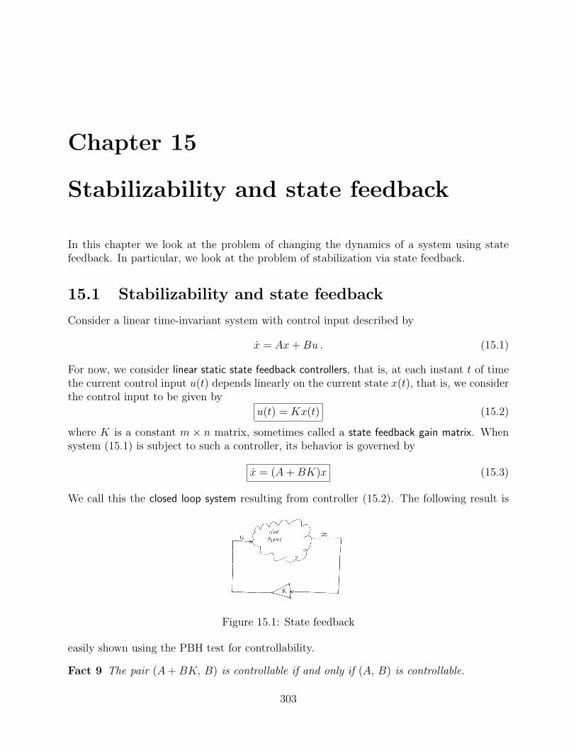
Chapter 15

Stabilizability and state feedback

In this chapter we look at the problem of changing the dynamics of a system using statefeedback. In particular, we look at the problem of stabilization via state feedback.

15.1 Stabilizability and state feedback

Consider a linear time-invariant system with control input described by

x = Ax + Bu . (15.1)

For now, we consider linear static state feedback controllers, that is, at each instant t of timethe current control input u(t) depends linearly on the current state x(t), that is, we considerthe control input to be given by

u(t) = Kx(t) (15.2)

where K is a constant m × n matrix, sometimes called a state feedback gain matrix. Whensystem (15.1) is subject to such a controller, its behavior is governed by

x = (A + BK)x (15.3)

We call this the closed loop system resulting from controller (15.2). The following result is

Figure 15.1: State feedback

easily shown using the PBH test for controllability.

Fact 9 The pair (A + BK, B) is controllable if and only if (A, B) is controllable.

303

Suppose the open loop system, that is, the system with zero feedback, or, x = Ax isunstable or at most marginally stable. A natural question is the following. Can we choosethe gain matrix K so that A + BK is asymptotically stable? If yes, we say that system(15.1) is stabilizable.

DEFN.[Stabilizability] System (15.1) is stabilizable if there exists a matrix K such that A+BKis asymptotically stable.

We sometimes say that the pair (A, B) is stabilizable if system (15.1) is stabilizable.The big question is: under what conditions is a given pair (A,B) stabilizable? We shall

see in Section 15.4.2 that controllability is a sufficient condition for stabilizability; that is,if a system is controllable it is stabilizable. However, controllability is not necessary forstabilizability, that is, it is possible for a system to be stabilizable but not controllable. Tosee this, consider a system with A asymptotically stable and B equal to zero; see also thenext two examples.

Example 190 (Not stabilizable and not controllable)

x1 = x1

x2 = u

For any gain matrix K, the matrix

A + BK =

(1 0k1 k2

)

has eigenvalues 1 and k2. Hence, A + BK is unstable for all K. So, this system is notstabilizable.

Example 191 (Stabilizable but not controllable.)

x1 = −x1

x2 = u

For any gain matrix K, the matrix

A + BK =

( −1 0k1 k2

)

has eigenvalues −1 and k2. Hence, A + BK is asymptotically stable provided k2 < 0. So,this system is stabilizable. However, it is not controllable.

15.2 Eigenvalue placement (pole placement) by state

feedback

Recall the stabilizability problem for the system

x = Ax + Bu

304

and suppose A and B are real matrices. Here we consider a more general question: Canwe arbitrarily assign the eigenvalues of A + BK by choice of the gain matrix K? The mainresult of this section is that the answer is yes if and only if the pair (A,B) is controllable.We consider first single input systems.

15.2.1 Single input systems

Here we consider scalar input (m = 1) systems. We first demonstrate that the characteristicpolynomial of A + BK depends in an affine linear fashion on the gain matrix K. To achievethis, we need to use the following result whose proof is given in the appendix at the end ofthis chapter.

Fact 10 Suppose M and N are any two matrices of dimensions n×m and m×n, respectively.Then,

det(I + MN) = det(I + NM) .

In particular, if m = 1, we have

det(I + MN) = 1 + NM .

Whenever s is not an eigenvalue of A, we have sI−A−BK = (sI−A)(I−(sI−A)−1BK).Thus, using Fact 10, we obtain that

det(sI − A−BK) = det(sI − A) det(I − (sI − A)−1BK)

= det(sI − A) det(I −K(sI − A)−1B)

= det(sI − A)(1−K(sI − A)−1B) ,

that is, the characteristic polynomial of A + BK satisfies

det(sI − A−BK) = det(sI − A)(1−K(sI − A)−1B) . (15.4)

From this expression, we can make the following statement:

For a single input system, the characteristic polynomial of A + BK depends in an affinelinear fashion on the gain matrix K.

We now show that we can arbitrarily assign the eigenvalues of A + BK by choice of thegain matrix K if (A,B) is controllable. Consider any bunch of complex numbers λ1, . . . , λn

with the property that if λ is in the bunch then so is λ and suppose we wish to choose a gainmatrix K such that the eigenvalues of A + BK are precisely these complex numbers. Let

d(s) =n∏

i=1

(s− λi)

that is, d is the unique monic polynomial whose roots are the desired closed loop eigenvalues,λ1, . . . , λn. We need to show that there is a gain matrix K so that det(sI−A−BK) = d(s).

305

Let d be the characteristic polynomial of A, that is, d(s) = det(sI − A). Then, recalling(15.4) we need to show that there exists a gain matrix K such that

d(s) = d(s)(1−K(sI − A)−1B)

that is,d(s)K(sI − A)−1B = d(s)− d(s) . (15.5)

Let

d(s) = a0 + a1s + · · ·+ an−1sn−1 + sn

d(s) = a0 + a1s + · · ·+ an−1sn−1 + sn .

Recall the power series expansion for (sI − A)−1:

(sI − A)−1 =1

sI +

1

s2A + · · ·+ 1

skAk−1 + · · ·

Substituting this expression into (15.5) and equating the coefficients of like powers of s weobtain that (15.5) holds if and only if

s0 : a1KB + a2KAB + · · ·+ an−1KAn−2B + KAn−1B = a0 − a0

s1 : a2KB + · · ·+ an−1KAn−3B + KAn−2B = a1 − a1...

sn−2 an−1KB + KAB = an−2 − an−2

sn−1 : KB = an−1 − an−1

that is,(

KB KAB · · · KAn−1B)Υ =

(a0 − a0 a1 − a1 · · · an−1 − an−1

)(15.6)

where Υ is the invertible matrix given by

Υ =

a1 a2 · · · an−2 an−1 1a2 a3 · · · an−1 1 0a3 a4 · · · 1 0 0...

......

......

an−1 1 · · · 0 0 01 0 . . . 0 0 0

. (15.7)

Let Qc be the controllability matrix associated with (A, B), that is,

Qc =(

B AB · · · An−1B)

.

Then condition (15.6) on K reduces to

KQcΥ =(

a0 − a0 a1 − a1 · · · an−1 − an−1

).

Because the pair (A,B) is controllable, Qc is invertible. This readily implies that the gainmatrix K is uniquely given by

K =(

a0 − a0 a1 − a1 · · · an−1 − an−1

)Υ−1Q−1

c . (15.8)

We have just demonstrated the following result.

306

Theorem 23 (Pole placement theorem: SI case) Suppose the real matrix pair (A,B)is a single input controllable pair with state dimension n and λ1, . . . , λn is any bunch of ncomplex numbers with the property that if λ is in the bunch then so is λ. Then there exists areal matrix K such that λ1, . . . , λn are the eigenvalues (multiplicities included) of A + BK.

MATLAB

>> help acker

ACKER Pole placement gain selection using Ackermann’s formula.

K = ACKER(A,B,P) calculates the feedback gain matrix K such that

the single input system

.

x = Ax + Bu

with a feedback law of u = -Kx has closed loop poles at the

values specified in vector P, i.e., P = eig(A-B*K).

See also PLACE.

Note: This algorithm uses Ackermann’s formula. This method

is NOT numerically reliable and starts to break down rapidly

for problems of order greater than 10, or for weakly controllable

systems. A warning message is printed if the nonzero closed loop

poles are greater than 10% from the desired locations specified

in P.


A =

(3 −24 −3

)and B =

(23

)

Here the controllability matrix

Qc =(

B AB)

=

(2 03 −1

)

is full rank; hence (A,B) is controllable. Considering any state feedback gain matrix K =(k1 k2

), we have

A + BK =

(3 + 2k1 −2 + 2k2

4 + 3k1 −3 + 3k2

)

and

det(sI − A−BK) = s2 − (2k1 + 3k2)s− 1 + k2 .

307

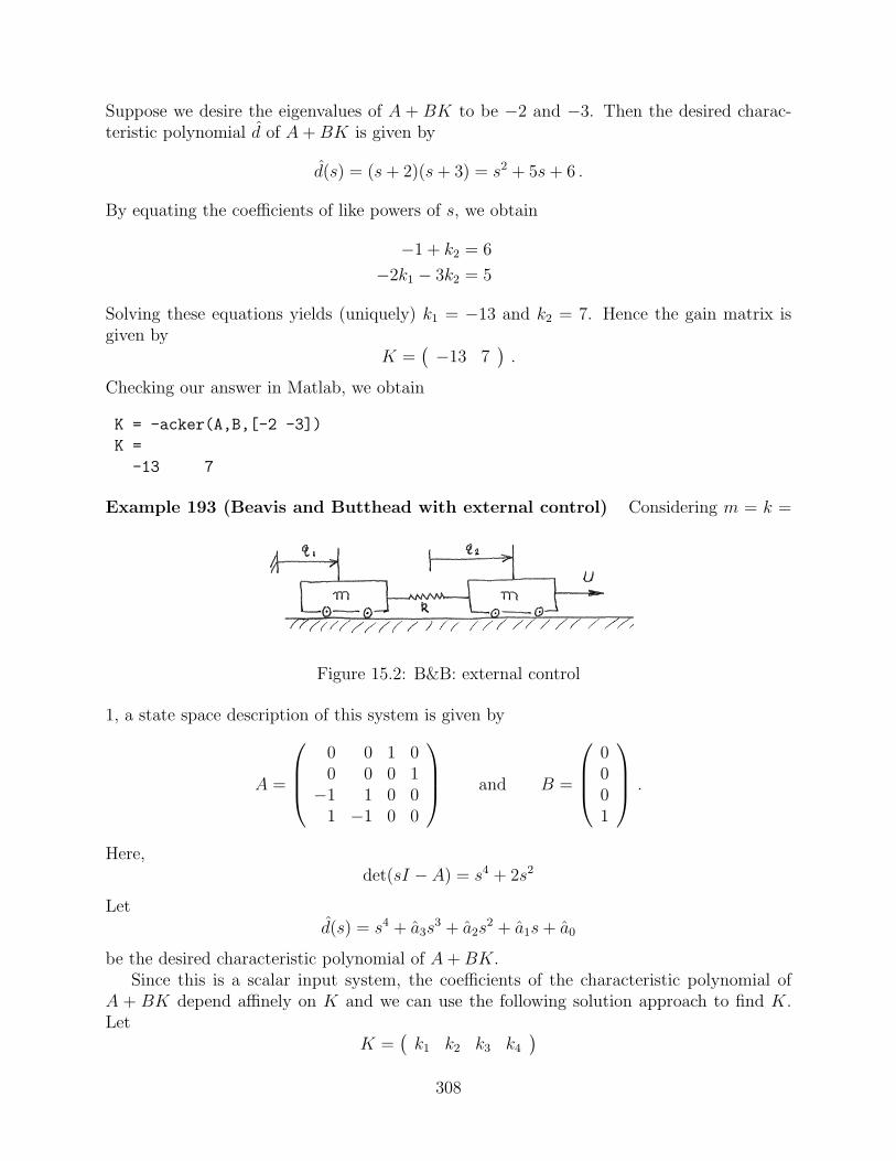
Suppose we desire the eigenvalues of A + BK to be −2 and −3. Then the desired charac-teristic polynomial d of A + BK is given by

d(s) = (s + 2)(s + 3) = s2 + 5s + 6 .

By equating the coefficients of like powers of s, we obtain

−1 + k2 = 6

−2k1 − 3k2 = 5

Solving these equations yields (uniquely) k1 = −13 and k2 = 7. Hence the gain matrix isgiven by

K =( −13 7

).

Checking our answer in Matlab, we obtain

K = -acker(A,B,[-2 -3])

K =

-13 7

Example 193 (Beavis and Butthead with external control) Considering m = k =

Figure 15.2: B&B: external control

1, a state space description of this system is given by

A =

0 0 1 00 0 0 1

−1 1 0 01 −1 0 0

and B =

0001

.

Here,det(sI − A) = s4 + 2s2

Letd(s) = s4 + a3s

3 + a2s2 + a1s + a0

be the desired characteristic polynomial of A + BK.Since this is a scalar input system, the coefficients of the characteristic polynomial of

A + BK depend affinely on K and we can use the following solution approach to find K.Let

K =(

k1 k2 k3 k4

)

308

Then

det(sI − A−BK) = det

s 0 −1 00 s 0 −11 −1 s 0

−1− k1 1− k2 −k3 s− k4

= s4 − k4s3 + (2− k2)s

2 − (k3 + k4)s− (k1 + k2) .

Note the affine dependence of the coefficients of the above polynomial on K. Letting theabove polynomial equal the desired polynomial d and equating like coefficients results in thefollowing four linear equations in the four unknowns components of K:

−k4 = a3

2− k2 = a2

−k3 − k4 = a1

−k1 − k2 = a0

Solving for k1, . . . , k4 uniquely yields

k1 = −2− a0 + a2

k2 = 2− a2

k3 = −a1 + a3

k4 = −a3

• To illustrate MATLAB, consider desired closed loop eigenvalues: −1,−2− 3,−4.

>> poles=[-1 -2 -3 -4];

>> poly(poles)

ans =

1 10 35 50 24

Hencea0 = 24 a1 = 50 a2 = 35 a3 = 10

and the above expressions for the gain matrix yield

k1 = 9 k2 = −33 k3 = −40 k4 = −10

Using MATLAB pole placement commands, we obtain:

>> k= place(a,b,poles)

place: ndigits= 18

k =

309

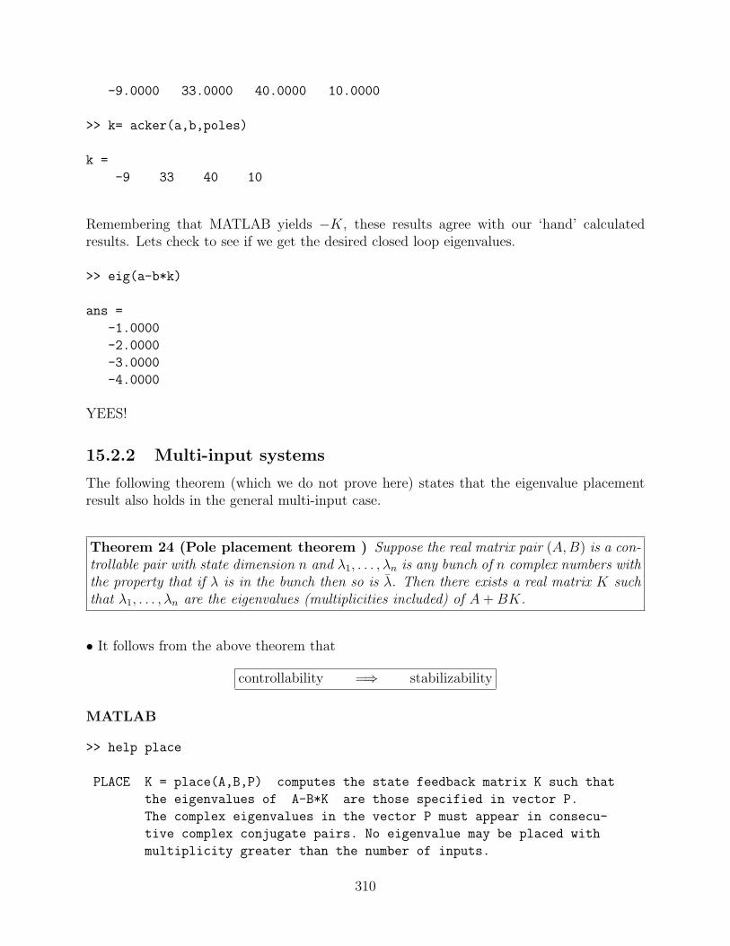
-9.0000 33.0000 40.0000 10.0000

>> k= acker(a,b,poles)

k =

-9 33 40 10

Remembering that MATLAB yields −K, these results agree with our ‘hand’ calculatedresults. Lets check to see if we get the desired closed loop eigenvalues.

>> eig(a-b*k)

ans =

-1.0000

-2.0000

-3.0000

-4.0000

YEES!

15.2.2 Multi-input systems

The following theorem (which we do not prove here) states that the eigenvalue placementresult also holds in the general multi-input case.

Theorem 24 (Pole placement theorem ) Suppose the real matrix pair (A,B) is a con-trollable pair with state dimension n and λ1, . . . , λn is any bunch of n complex numbers withthe property that if λ is in the bunch then so is λ. Then there exists a real matrix K suchthat λ1, . . . , λn are the eigenvalues (multiplicities included) of A + BK.

• It follows from the above theorem that

controllability =⇒ stabilizability

MATLAB

>> help place

PLACE K = place(A,B,P) computes the state feedback matrix K such that

the eigenvalues of A-B*K are those specified in vector P.

The complex eigenvalues in the vector P must appear in consecu-

tive complex conjugate pairs. No eigenvalue may be placed with

multiplicity greater than the number of inputs.

310

The displayed "ndigits" is an estimate of how well the

eigenvalues were placed. The value seems to give an estimate

of how many decimal digits in the eigenvalues of A-B*K match

the specified numbers given in the array P.

A warning message is printed if the nonzero closed loop poles

are greater than 10% from the desired locations specified in P.

See also: LQR and RLOCUS.

311

15.3 Uncontrollable eigenvalues (you can’t touch them)

In the previous section, we saw that, if the pair (A,B) is controllable, then one couldarbitrarily place the eigenvalues of A + BK by appropriate choice of the gain matrix K;hence controllability is a sufficient condition for arbitrary eigenvalue placement. In thissection, we show that controllability is also necessary for arbitrary eigenvalue placement.In particular, we show that if λ is an uncontrollable eigenvalue of (A,B), then λ is aneigenvalue of A + BK for every K. Recall Examples 190 and 191 in which the matrix Ahad an eigenvalue λ with the property that for every gain matrix K, it is an eigenvalue ofA + BK. We now demonstrate the following result:

If λ is an uncontrollable eigenvalue of (A,B), then λ is an eigenvalue of A+BK for everygain matrix K.

To see this, recall that λ is an uncontrollable eigenvalue of (A,B) if and only if

rank(

A− λI B)

< n (15.9)

where A is n× n. Hence, there exists a nonzero n-vector w such that

w′ ( A− λI B)

= 0 .

that isw′(A− λI) = 0 and w′B = 0

So, for any gain matrix K, we have

w′(A + BK) = λw′

that is, λ is an eigenvalue of A + BK with left eigenvector w. So, regardless of the feed-back gain matrix, λ is always an eigenvalue of A + BK. We cannot alter this eigenvalueby feedback. In particular, if λ has a non-negative real part, then the pair (A,B) is notstabilizable.

Another way to see the above result is to consider the nice transformation introducedearlier, namely,

x = T x and x =

(xc

xu

)

which results in the equivalent system description,

˙x = Ax + Bu

where

A = T−1AT =

(Acc Acu

0 Auu

)and B = T−1B =

(Bc

0

)

312

and the pair (Acc, Bc) is controllable. If u = Kx, then u = Kx where K = KT . LettingK =

(Kc Ku

), we obtain

A = BK =

(Acc + BcKc Acu + BcKu

0 Auu

)

SinceA + BK = T−1[A + BK]T

the eigenvalues of A + BK are exactly the same as those of A + BK which are equal to theunion of the eigenvalues of Acc + BcKc and Auu. From this we see that, regardless of K, theeigenvalues of Auu are always eigenvalues of A+BK. Now recall that the eigenvalues of Auu

are the uncontrollable eigenvalues of (A,B).Furthermore, since the pair (Acc, Bc) is controllable, the eigenvalues of Acc + BcKc can

be arbitrarily placed by appropriate choice of Kc. Hence, except for the eigenvalues of Auu,all eigenvalues of A + BK can be arbitrarily placed. In particular, if all the eigenvalues ofAuu have negative real parts, then K can be chosen so that all the eigenvalues of A + BKhave negative real parts. So, we have the following conclusion.

A pair (A,B) is stabilizable if and only if all the uncontrollable eigenvalues of (A,B) havenegative real parts.

Recalling the PBH test for uncontrollable eigenvalues, we now have the following PBHresult on stabilizability.

Theorem 25 (PBH stabilizability theorem) A pair (A,B) is stabilizable if and onlyif

rank (A− λI B) = n

for every eigenvalue λ of A with nonnegative real part.

Example 194A =

0 -1 0

1 -1 -1

-1 0 0

B =

1

-1

1

rank(ctrb(A,B))

2 %Uncontrollable

eig(A)

313

0 + 1.0000i

0 - 1.0000i

-1.0000

rank([ A-i*eye(3) B])

3 %Stabilizable

rank([ A+eye(3) B])

2 %-1 is an uncontrollable eigenvalue

Considering K =(

k1 k2 k3

)we obtain that

det(sI − A−BK) = s3 + (1− k1 + k2 − k3)s2 + (1− 2k1)s + (1− k1 − k2 + k3) .

As expected, we can write this as

det(sI − A−BK) = (s + 1)(s2 + (−k1 + k2 − k3)s + (1− k1 − k2 + k3)

)

Suppose that the desired eigenvalues of A + BK are −1− 2,−3. Then

d(s) = (s + 1)(s + 2)(s + 3) = s3 + 6s2 + 11s + 6 .

Equating coefficients, we obtain

1− k1 − k2 + k3 = 6

1− 2k1 = 11

1− k1 + k2 − k3 = 6

Solving yields

k1 = −5

k2 = k3

k3 is arbitrary

We choose

K =( −5 0 0

).

eig(A+B*K)

-3.0000

-2.0000 %Just checking!

-1.0000

314

Remark 9 If system (15.1) is not stabilizable via a linear static state controller of the formu = Kx then, it is not stabilizable with any controller. This can be seen as follows. Thefact that the system is not stabilizable via a linear controller implies that the system has anuncontrollable eigenvalue λ with non-negative real part. Hence there exists a nonzero vectorw such that, regardless of the input u, we have

w′x(t) = eλtw′x(0)

for all t. Considering any initial state x(0) for which w′x(0) 6= 0 (for example, let x(0) bethe real part of w), we see that, regardless of the input u, the resulting solution x(t) doesnot go to zero as t goes to infinity.

15.4 Controllable canonical form

Consider a scalar input system of the form x = Ax + Bu where A and B have the followingstructure:

A =

0 1 0 . . . 0 00 0 1 . . . 0 0...

.... . .

......

.... . .

...0 0 0 . . . 0 1−a0 −a1 −a2 . . . −an−2 −an−1

and B =

00......01

.

We say that the pair (A,B) is in controllable canonical form. We saw this structure when weconstructed realizations for scalar transfer functions. Note that x = Ax + Bu looks like:

x1 = x2

...

xn−1 = xn

xn = −a0x1 + a1x2 + . . . + an−1xn + u

Also,det(sI − A) = a0 + a1s + · · ·+ an−1s

n−1 + sn

Example 195 (Controlled unattached mass)

x1 = x2

x2 = u

Here,

A =

(0 10 0

)and B =

(01

).

315

Fact 11 If the pair (A,B) is in controllable canonical form, then it is controllable.

To prove the above result, let K =(

a0 a1 · · · an−1

). Then

A + BK =

0 1 0 . . . 0 00 0 1 . . . 0 0...

.... . .

......

.... . .

...0 0 0 . . . 0 10 0 0 . . . 0 0

The controllability matrix Qc for the pair (A + BK,B) is simply given by

Qc =

0 0 · · · 0 10 0 · · · 1 0...

.... . . 0 0

0 1 · · · 0 01 0 · · · 0 0

This matrix has rank n; hence (A + BK, B) is controllable. It now follows that (A,B) iscontrollable.

15.4.1 Transformation to controllable canonical form∗

Here we show that any controllable single-input system

x = Ax + Bu

can be transformed via a state transformation to a system which is in controllable canonicalform.

State transformations. Suppose T is a nonsingular matrix and consider the state trans-formation

x = T x

Then the evolution of x is governed by

˙x = Ax + Bu

where A = T−1AT and B = T−1B.

Note that controllability is invariant under a state transformation, that is, (A,B) iscontrollable if and only if (T−1AT, T−1B) is controllable. This can readily seen by notingthe controllability matrix Qc for the pair (T−1AT, T−1B) is given by Qc = T−1Qc where Qc

is the controllability matrix for (A,B); hence Qc and Qc have the same rank.

316

Transformation to controllable canonical form. Suppose (A,B) is controllable andm = 1. Then the following algorithm yields a state transformation which transforms (A, B)into controllable canonical form.

Algorithm. Leta0 + . . . + an−1s

n−1 + sn = det(sI − A)

Recursively define the following sequence of n-vectors:

tn = Btj = Atj+1 + ajB , j = n− 1, . . . , 1

and letT =

(t1 . . . tn

)

Fact 12 If (A,B) is controllable then, the matrix T is generated by the above algorithm isnonsingular and the pair (T−1AT, T−1B) is in controllable canonical form.

Proof. We first need to prove that T is nonsingular. By applying the algorithm, we obtain

tn = Btn−1 = AB + an−1Btn−2 = A(AB + an−1B) + an−2B = A2B + an−1AB + an−2B

One may readily show by induction that for j = n− 1, n− 2 · · · , 1, one has

tj = An−jB + an−1An−j−1B + · · ·+ aj+1AB + ajB (15.10)

From this it should be clear that for any j = n, n− 1, · · · 1,

rank(

tn tn−1 · · · tj)

= rank(

B AB · · · An−jB)

Hence

rankT = rank(

tn tn−1 · · · t1)

= rank(

B AB · · · AnB)

= rankQc

Since (A,B) is controllable, Qc has rank n. Hence T has rank n and is invertible.We now show that T−1AT and T−1B have the required structure. It follows from (15.10)

thatt1 = An−1B + an−1A

n−2B + · · ·+ a2AB + a1B

Using the Cayley Hamilton Theorem, we obtain

At1 = [An + an−1An−1 + · · ·+ a2A

2 + a1A]B = −a0B ,

that is At1 = −a0tn. Also from the algorithm, we have

Atj = tj−1 − aj−1tn for j = 2, 3, · · · , n

Recalling a useful fact on similarity transformations, it follows that T−1AT has the requiredstructure. Since B = tn, it follows that T−1B also has the required structure.

We can now state the following result.

317

Theorem 26 A single input system (A,B) is controllable if and only if there is a nonsingularmatrix T such that (T−1AT, T−1B) is in controllable canonical form.

Example 196 (Beavis and Butthead with external control.) Consider m = k = 1. Then,

A =

0 0 1 00 0 0 1

−1 1 0 01 −1 0 0

and B =

0001

.

Hence,det(sI − A) = s4 + 2s2

andt4 = B

t3 = At4 + a3B = At4 =

0100

t2 = At3 + a2B = At3 + 2B =

0011

t1 = At2 + a1B = At2 =

1100

So, the transformation matrix is given by:

T =(

t1 t2 t3 t4)

=

1 0 0 01 0 1 00 1 0 00 1 0 1

>> inv(t)

ans =

1 0 0 0

0 0 1 0

-1 1 0 0

0 0 -1 1

>> inv(t)*a*t

ans =

0 1 0 0

0 0 1 0

318

0 0 0 1

0 0 -2 0

15.4.2 Eigenvalue placement by state feedback∗

Recall that if (A,B) is controllable then, we arbitrarily assign the eigenvalues of A + BKby choice of the gain matrix K? We can demonstrate this result for single input systemsusing the controllable canonical form. Consider any bunch of complex numbers λ1, . . . , λn

with the property that if λ is in the bunch then so is λ and suppose we wish to choose again matrix K such that the eigenvalues of A + BK are precisely these complex numbers.

Let

d(s) = sn + an−1sn−1 + . . . + a0 =

n∏i=1

(s− λi)

that is, the real numbers, a0, . . . , an−1, are the coefficients of the unique monic polynomial dwhose roots are the desired closed loop eigenvalues, λ1, . . . , λn. If (A, B) is controllable andm = 1, then there exists a nonsingular matrix T such that the pair (A, B) is in controllablecanonical form, where A = T−1AT and B = T−1B, that is,

A =

0 1 0 . . . 0 00 0 1 . . . 0 0...

.... . .

......

.... . .

...0 0 0 . . . 0 1−a0 −a1 −a2 . . . −an−2 −an−1

, B =

00......01

where

sn + an−1sn−1 + . . . + a0 = det(sI − A) .

Considering the 1× n real gain matrix

K =(

a0−a0 a1−a1 . . . an−1−an−1

)

we obtain

A + BK =

0 1 0 . . . 0 00 0 1 . . . 0 0...

.... . .

......

.... . .

...0 0 0 . . . 0 1−a0 −a1 −a2 . . . −an−2 −an−1

.

Clearly, the matrix A + BK has the desired characteristic polynomial d. Let

K = KT−1 .

319

Then

A + BK = TAT−1 + TBKT−1

= T [A + BK]T−1

and hencedet(sI − A−BK) = det(sI − A− BK) = d(s)

in other words, the eigenvalues of A + BK are as desired.

Remark 10 For scalar input systems, the coefficients of the characteristic polynomial ofA + BK depend affinely on K. Since K = KT−1, it follows that the coefficients of thecharacteristic polynomial of A + BK depend affinely on K.

Example 197 (Beavis and Butthead with external control) Here

A =

0 0 1 00 0 0 1

−1 1 0 01 −1 0 0

and B =

0001

.

We have already shown that this system is controllable and it can be transformed to con-trollable canonical form with the matrix

T =

1 0 0 01 0 1 00 1 0 00 1 0 1

Also,det(sI − A) = s4 + 2s2

Letp(s) = s4 + a3s

3 + a2s2 + a1s + a0

be the desired characteristic polynomial of A + BK. Then

K =( −a0 −a1 2−a2 −a3

)

and

K = = KT−1 =( −a0 −a1 2−a2 −a3

)

1 0 0 00 0 1 0

−1 1 0 00 0 −1 1

=( −2−a0+a2 2−a2 −a1 + a3 −a3

)

This is the same as the result we previously obtained for this example.

320

15.5 Discrete-time systems

Basically, everything we have said in this chapter so far also holds for discrete time systems,except that in talking about asymptotic stability of discrete-time systems, we need theeigenvalues to have magnitude strictly less than one.

15.5.1 Dead beat controllers

One cannot drive the state of a LTI continuous-time system to zero in a finite time using astatic linear state-feedback controller. However, this is possible for a controllable discrete-time system. To see this, consider

x(k+1) = Ax(k) + Bu(k)

where x(k) is an n-vector and u(k) is an m-vector and suppose that the pair (A,B) is con-trollable. Then there exists a gain matrix K so that all the eigenvalues of the correspondingclosed loop system matrix Acl := A + BK are all zero. Hence the characteristic polynomialof Acl is p(s) = sn. From the Cayley-Hamilton Theorem, we obtain that

Ancl = 0 .

Since the solutions x(·) of the closed lop system

x(k+1) = Aclx(k)

satisfy x(k) = Akclx(0) for all k ≥ 0, we see that

x(k) = 0 for k ≥ n .

Thus, all solutions go to zero in at most n steps.

Application to continuous-time systems. One could use the above result to obtain acontroller which drives the state of a continuous-time system to zero. Simply, pick a samplingtime T and discretize the continuous-time system. Now design a deadbeat controller for thediscrete-time system. Using a zero order hold, apply this controller to the continuous-timesystem. Note that the resulting controller is not a static controller for the continuous-timesystem.

321

15.6 Stabilization of nonlinear systems

Consider a nonlinear system described by

x = F (x, u)

and suppose we wish to stabilize this system about some controlled equilibrium state xe.Let ue be a constant input that achieves the desired controlled equilibrium state xe, that is,F (xe, ue) = 0. Let

δx = Aδx + Bδu (15.11)

be the linearization of the nonlinear system about (xe, ue). Thus,

A =∂F

∂x(xe, ue) and B =

∂F

∂u(xe, ue) .

15.6.1 Continuous-time controllers

If the pair (A, B) is stabilizable, the following procedure yields a controller which stabilizesthe nonlinear system about xe.

Choose a gain matrix K such that all eigenvalues of A + BK have negative real part andlet

u = ue + K(x− xe) (15.12)

We now show that the above controller results in the closed loop nonlinear system beingasymptotically about xe. To this end, note that the closed loop system is described by

x = f(x) = F (x, Kx + ue−Kxe)

Note that

f(xe) = F (xe, ue) = 0 ;

hence xe is an equilibrium state for the closed loop system. Linearizing the closed loopsystem about xe, we obtain

δx = (A + BK)δx

Since all the eigenvalues of A+BK have negative real parts, the closed loop nonlinear systemis asymptotically stable about xe.

15.6.2 Discrete-time controllers

Linearize the continuous time nonlinear system to obtain the LTI continuous-time system(15.11).

Choose a sample time T > 0 and discretize (15.11) to obtain

δxd(k+1) = Adδxd(k) + Bdδud(k) (15.13)

322

If the pair (Ad, Bd) is stabilizable, choose matrix K so that all the eigenvalues of Ad + BdKhave magnitude less than one.

Letud(k) = K(xd(k)− xe) + ue = K[x(kT )− xe] + ue . (15.14)

The continuous control input u is obtained form ud via a zero order hold.

Exercises

Exercise 124 Consider the system with input u, output y, and state variables x1, x2, x3, x4

described by

x1 = −x1

x2 = x1 − 2x2

x3 = x1 − 3x3 + u

x4 = x1 + x2 + x3 + x4

y = x3

(a) Is this system controllable?(b) Is this system stabilizable using state feedback? Justify your answers.

Exercise 125 (BB in laundromat: external excitation.) Obtain a state space representationof the following system.

mφ1 −mΩ2φ1 + k2(φ1 − φ2) = 0

mφ2 −mΩ2φ2 − k2(φ1 − φ2) = u

Show that this system is controllable.Considering

Ω = 1, m = 1, k = 2

obtain a linear state feedback controller which results in a closed loop system with eigenvalues

−1,−2,−3,−4

Use the following methods.

(a) Method based on computing the transformation matrix which transforms to control-lable canonical form.

(b) Obtaining an expression for the closed loop characteristic polynomial in terms of thecomponents of the gain matrix.

(c) acker

(d) place

323

Numerically simulate the closed loop system with the same initial conditions you used in tosimulate the open-loop system.

Exercise 126 Consider the system described by

x1 = x31 + sin x2 − 1 + u

x2 = −ex1 + (cos x2)u

Obtain a state feedback controller which results in a closed loop system which is asymptoti-cally stable about the zero state.

Exercise 127 Stabilization of 2-link manipulator with linear state feedback.

[m1lc21 + m2l

21 + I1]q1 + [m2l1lc2 cos(q1 − q2)]q2 + m2l1lc2 sin(q1 − q2)q

22

− [m1lc1 + m2l1]g sin(q1) = u

[m2l1lc2 cos(q1 − q2)]q1 + [m2lc22 + I2]q2 −m2l1lc2 sin(q1 − q2)q

21 −m2glc2 sin(q2) = 0

Linearize this system aboutq1 = q2 = u = 0

and obtain a state space description.For rest of exercise, use MATLAB and the following data: Is the linearization control-

m1 l1 lc1 I1 m2 l2 lc2 I2 mpayload

kg m m kg.m2 kg m m kg.m2 kg

10 1 0.5 10/12 5 1 0.5 5/12 0

lable? Design a state feedback controller which stabilizes this linearized system . Apply thecontroller to the nonlinear system and simulate the nonlinear closed loop system for variousinitial conditions.


x1 = x2 + u

x2 = x1 + u

(a) Is this system stabilizable ?

(b) Does there exist a linear state feedback controller which results in closed loop eigen-values −1,−2?

(b) Does there exist a linear state feedback controller which results in closed loop eigen-values −2,−3?

In parts (b) and (c): If no controller exists, explain why; if one does exist, give an exampleof one.

324


x1 = −x2 + u

x2 = −x1 − u

where all quantities are scalars.

(a) Is this system stabilizable via state feedback?

(b) Does there exist a linear state feedback controller which results is closed loop eigenval-ues −1,−4?

(c) Does there exist a linear state feedback controller which results is closed loop eigenval-ues −2,−4?

In parts (b) and (c): If no controller exists, explain why; if one does exist, give an exampleof one.

Exercise 130 Consider the system

x1 = x2

x2 = −x1 + u

(a) Design a continuous-time linear state feedback controller which stabilizes this systemabout the zero state. Illustrate the effectiveness of your controller with a simulation.

(b) For various sampling times, discretize the controller found in part (a) and simulate thecorresponding closed loop. Is the closed loop system stable for any sampling time?

(c) Design a stabilizing discrete-time controller based on a discretization of the system.Consider sampling times T = 0.1, 1, 2π, 10. Illustrate the effectiveness of your controllerwith simulations of the continuous-time system subject to the discrete-time controller.

(d) Design a dead-beat controller based on a discretization of the system. Consider sam-pling times T = 0.1, 1, 10. Illustrate the effectiveness of your controller with simula-tions.

Exercise 131 (BB in laundromat: external excitation.) Obtain a state space representationof the following system.

mφ1 −mΩ2φ1 + k2(φ1 − φ2) = 0

mφ2 −mΩ2φ2 − k2(φ1 − φ2) = u

(a) Show that this system is controllable.(b) Considering

Ω = 1, m = 1, k = 2

obtain a linear state feedback controller which results in a closed loop system with eigenvalues

−1,−2,−3,−4


325

(i) Obtain (by hand) an expression for the closed loop characteristic polynomial in termsof the components of the gain matrix.

(ii) acker

(iii) place

Illustrate the effectiveness of your controllers with numerical simulations.

Exercise 132 (Stabilization of cart pendulum system via state feedback.) Carry outthe following for parameter sets P2 and P4 and equilibriums E1 and E2. Illustrate the ef-fectiveness of your controllers with numerical simulations.

Using eigenvalue placement techniques, obtain a state feedback controller which stabilizesthe nonlinear system about the equilibrium.

What is the largest value of δ (in degrees) for which your controller guarantees conver-gence of the closed loop system to the equilibrium for initial condition

(y, θ1, θ2, y, θ1, θ2)(0) = (0, θe1−δ, θe

2+δ, 0, 0, 0)

where θe1 and θe

2 are the equilibrium values of θ1 and θ2.

Exercise 133 (Discrete-time stabilization of cart pendulum system via state feedback.)Carry out the following for parameter set P4 and equilibriums E1 and E2. Illustrate theeffectiveness of your controllers with numerical simulations.

Using eigenvalue placement techniques, obtain a discrete-time state feedback controllerwhich stabilizes the nonlinear system about the equilibrium.

What is the largest value of δ (in degrees) for which your controller guarantees conver-gence of the closed loop system to the equilibrium for initial condition

(y, θ1, θ2, y, θ1, θ2)(0) = (0, θe1−δ, θe

2+δ, 0, 0, 0)

where θe1 and θe

2 are the equilibrium values of θ1 and θ2.

15.7 Appendix

Proof of Fact 10. We need to prove that for any two matrices M and N of dimensionsm× n and n×m, respectively, we have

det(I + MN) = det(I + NM) .

Consider the following matrix equation:

(I M−N I

)(I ON I

)=

(I + MN M

O I

)(15.15)

Since the matrix on the right of the equality is block diagonal, its determinant is det(I) det(I+MN) = det(I + MN). Hence the product of the determinants of the two matrices on the

326

left of the equation is det(I + MN). Reversing the order of the two matrices on the left of(15.15), we obtain (

I ON I

)(I M−N I

)=

(I MO I + NM

)

From this we can conclude that the product of the determinants of the two matrices on the leftof equation (15.15) is det(I +NM). Hence we obtain the desired result that det(I +MN) =det(I + NM).

327

Chapter 16

Detectability and observers

16.1 Observers, state estimators and detectability

Consider the system (we will call it the plant)


(16.1)

Suppose that at each instant time t we can measure the plant output y(t) and the plantinput u(t) and we wish to estimate the plant state x(t). In this section we demonstrate howto obtain an estimate x(t) of the plant state x(t) with the property that as t →∞ the stateestimation error x(t) − x(t) goes to zero. We do this by constructing an observer or stateestimator.

Observer or state estimator. An observer or state estimator for a plant is a systemwhose inputs consist of the plant input and plant output while its output is an estimate ofthe plant state; see Figure 16.1.

Figure 16.1: Observer

We consider here observers which have the following structure.

˙x = Ax + Bu + L(y − y)y = Cx + Du

x(0) = x0 (16.2)

where the n-vector x(t) is the estimated state; the matrix L is called the observer gain matrixand is yet to be determined. The initial state x0 for the observer is arbitrary. One can regardx0 as an initial guess of the initial plant state x0.

329

Note that the observer consists of a copy of the plant plus the “correction term,” L(y−y).

If we rewrite the observer description as

˙x = (A + LC)x + (B + LD)u− Ly ,

it should be clear that we can regard the observer as a linear system whose inputs are theplant input u and plant output y. We can regard the estimated state x as the observeroutput.

To discuss the behavior of the above estimator, we introduce the state estimation error

x := x− x

Using (16.1) and (16.2) one can readily show that the evolution of the estimation error issimply governed by

˙x = (A + LC)x

Hence, if one can choose L such that all the eigenvalues of the matrix A + LC have negativereal parts then, we obtain the desired result that

limt→∞

x(t) = 0 .

In other words, the state estimation error goes to zero as t goes to infinity. When thishappens, we call the observer an asymptotic observer. This leads to the next definition.

DEFN. System (16.1) or the pair (C, A) is detectable if there exists a matrix L such thatA + LC is asymptotically stable.

Note that the matrix A + LC is asymptotically stable if and only if the matrix

(A + LC)∗ = A∗ + C∗L∗

is asymptotically stable. Thus, the problem of choosing a matrix L so that A + LC isasymptotically stable is equivalent to the stabilizability problem of choosing K so that A∗+C∗K is asymptotically stable. If one solves the stabilizability problem for K, then L = K∗

solves the original problem.From the above observations, we obtain the following duality between stabilizability and

detectability.

• (C, A) is detectable if and only if (A∗, C∗) is stabilizable.

• (A, B) is stabilizable if and only if (B∗, A∗) is detectable.

• Also, it follows that

observability =⇒ detectability

330

16.2 Eigenvalue placement for estimation error dynam-

ics

Suppose (C, A) is a real observable pair. Then (A∗, C∗) is a real controllable pair. Nowconsider any bunch of complex numbers

λ1, λ2, · · · , λn with the property that if λ is in the bunch then so is λ. Since (A∗, C∗) is real and controllable,there is a real gain matrix K such that λ1, λ2, · · · , λn are precisely the eigenvalues ofA∗ + C∗K. Letting L = K∗ and recalling that a matrix and its transpose have the sameeigenvalues, we obtain that the eigenvalues of A + LC are precisely λ1, λ2, · · · , λn . Wehave just demonstrated the following result.

If (C,A) is observable, one can arbitrarily place the eigenvalues of A + LC by appropriatechoice of the observer gain matrix L.

Example 198 (The unattached mass with position measurement and an input.)

x1 = x2

x2 = uy = x1

Here

A =

(0 10 0

)C =

(1 0

)

Since this system is observable, it is detectable. If

L =

(l1l2

)

we have

A + LC =

(l1 1l2 0

)

Hence,det(sI − A− LC) = s2 − l1s− l2

and A + LC is asymptotically stable if

l1 < 0 l2 < 0

An asymptotic observer is then given by

˙x1 = x2 + l1(x1 − y)˙x2 = u + l2(x1 − y)

and the estimation error x = x− x satisfies

˙x1 = l1x1 + x2

˙x2 = l2x1

331

16.3 Unobservable modes (you can’t see them)

Suppose system (16.1) is unobservable. Then, as we have already seen, this system will haveat least one unobservable eigenvalue λ. This means that, when u(t) ≡ 0, the system has anonzero solution of the form xuo(t) = eλtv which produces zero output, y(t) ≡ 0. Thus onecannot distinguish this state motion from the zero motion, x(t) ≡ 0. If <(λ) < 0 then xuo(t)asymptotically goes to zero. However, if <(λ) ≥ 0 then, xuo(t) does not asymptotically goto zero. Hence, even using nonlinear observers, there is no way that one can asymptoticallyestimate the state of this system. For linear observers, we have the following result.

If λ an unobservable eigenvalue of (C, A), then λ is an eigenvalue of A + LC for everyobserver gain matrix L .

To see this, recall that λ is an unobservable eigenvalue of (C, A) if and only if

rank

(A− λI

C

)< n

where A is n× n. Hence, there is a nonzero n-vector v such that(

A− λIC

)v = 0

or, equivalently,

Av = λv

Cv = 0

Hence, for any matrix L(A + LC)v = λv

Since v 6= 0, it follows that λ is an eigenvalue of A + LC.The next result states that a necessary and sufficient condition for stabilizability is that

all unobservable eigenvalues are asymptotically stable.

Theorem 27 (PBH detectability theorem) The pair (C, A) is detectable if and only if

rank

(A− λI

C

)= n

for every eigenvalue λ of A with nonnegative real part.

Proof. Use duality and the corresponding result for stabilizability.

Example 199 (The unattached mass with velocity measurement.)

x1 = x2

x2 = 0y = x2

332

Here

A =

(0 10 0

)C =

(0 1

)

Hence (A− λI

C

)=

−λ 1

0 −λ0 1

The above matrix has rank 1 < n for λ = 0; hence λ = 0 is an unobservable eigenvalue andthis system in not detectable.

Note that for any observer gain matrix

L =

(l1l2

)

we have

A + LC =

(0 1 + l10 l2

)

Hence,det(sI − A− LC) = s(s− l2)

So, regardless of choice of L, the matrix A + LC always has an eigenvalue at 0.

16.4 Observable canonical form*

Suppose A and C have the following structure:

A =

0 0 · · · 0 −a0

1 0 · · · 0 −a1

0 1 · · · 0 −a2...

. . ....

0 0 · · · 1 −an−1

and C =(

0 0 · · · 0 1)

.

Then we say that the pair (C,A) is in observable canonical form. Note that (C, A) is inobservable canonical form if and only if (A∗, C∗) is in controllable canonical form. If (C, A)is in observable canonical form, then x = Ax and y = Cx look like

x1 = −a0xn

x2 = −a1xn + x1...

xn = −an−1xn + xn−1

y = xn

Also,det(sI − A) = sn + an−1s

n−1 + · · ·+ a0 .

333

If we reverse the ordering of the states, then

x1 = −an−1x1 + x2...

xn−1 = −a1x1 + xn

xn = −a0x1

y = x1

and the corresponding A and C matrices have the following structure:

A =

−an−1 1 0 · · · 0−an−2 0 1 · · · 0

.... . .

...−a1 1 0 · · · 1−a0 0 0 · · · 0

and C =(

1 0 · · · 0 0)


The results for discrete-time systems are basically the same as those for continuous-timesystems. Consider a discrete-time system described by

x(k+1) = Ax(k) + Bu(k)y(k) = Cx(k) + Du(k)

(16.3)

Observer or state estimator. Recalling the observer structure in the continuous-timecase, we consider here observers which have the following structure.

x(k+1) = Ax(k) + Bu(k) + L(y(k)− y(k))y(k) = Cx(k) + Du(k)

x(0) = x0 (16.4)

where the n-vector x(k) is the estimated state; the matrix L is called the observer gain matrix.

Introducing the state estimation error

x := x− x

and using (16.3) and (16.4) one can readily show that the evolution of the estimation erroris simply governed by

x(k+1) = (A + LC)x(k)

Hence, if one can choose L such that all the eigenvalues of the matrix A+LC have magnitudeless than one then, we obtain the desired result that

limt→∞

x(k) = 0 .

334

Dead beat observer. If (C,A) is observable, choose L so that all the eigenvalues of A+LCare zero. Then, the state estimation error goes to zero in at most n steps.

Exercises

Exercise 134 BB in laundromat: Obtain a state space representation of the followingsystem.

mφ1 −mΩ2φ1 + k2(φ1 − φ2) = 0

mφ2 −mΩ2φ2 − k2(φ1 − φ2) = u

y = φ2

Show that this system is observable. Considering

Ω = 1, m = 1, k = 2

obtain a state estimator (observer) which results in an estimation error system with eigen-values

−1,−2,−3,−4


(a) Obtaining an expression for the characteristic polynomial of the error system in termsof the components of the observer gain matrix.

(b) acker

(c) place

Illustrate the effectiveness of your observer(s) with numerical simulations.


x1 = −x2 + u

x2 = −x1 − u

y = x1 − x2

where all quantities are scalars.

(a) Is this system observable?

(b) Is this system detectable?

(c) Does there exist an asymptotic state estimator for this system? If an estimator doesnot exist, explain why; if one does exist, give an example of one.

335

Chapter 17

Climax: output feedback controllers

Plant. (The object of your control desires.) Consider a system described by

x = Ax + Buy = Cx

(17.1)

where the state x(t) is an n-vector, the control input u(t) is an m-vector, and the measuredoutput y(t) is a p-vector. Initially, we consider D = 0 for simplicity of presentation.

17.1 Memoryless (static) output feedback

The simplest type of controller is a memoryless (or static) linear output feedback controller;this is of the form

u = Ky

where K is a real m × p matrix, sometimes called a gain matrix. This controller results inthe following closed loop system:

x = (A + BKC)x

If the open loop system x = Ax is not asymptotically stable, a natural question is whetherone can choose K so that the closed loop system is asymptotically stable. For full statefeedback (C = I), we have seen that it is possible to do this if (A, B) is controllable or, lessrestrictively, if (A,B) is stabilizable. If (C, A) is observable or detectable, we might expectto be able to stabilize the plant with static output feedback. This is not the case as thefollowing example illustrates.

Example 200 Unattached mass with position measurement.

x1 = x2

x2 = u

y = x1

This system is both controllable and observable. All linear static output feedback controllersare given by

u = ky

337

which results in

x1 = x2

x2 = kx1

Such a system is never asymptotically stable.Note that if the plant has some damping in it, that is,

x1 = x2

x2 = −dx2 + uy = x1

where d > 0, the closed loop system is given by

x1 = x2

x2 = kx1 − dx2

This is asymptotically stable provided k < 0.


x1 = x2

x2 = x1 + uy = −2x1 + x2

For a SISO system, one could use root locus techniques to determine whether or notthe system is stabilizable via static output feedback. For a general MIMO system, thereare currently are no easily verifiable conditions which are both necessary and sufficient forstabilizability via static output feedback. It is a topic of current research. So where do wego now?

17.2 Dynamic output feedback

A dynamic output feedback controller is a dynamic input-output system whose input is themeasured output of the plant and whose output is the control input to the plant. Thus, alinear, time-invariant, dynamic, output-feedback controller is described by

xc = Acxc + Bcyu = Ccxc + Dcy

(17.2)

338

where the nc-vector xc(t) is called the controller state and nc is the order of the controller. Weregard a memoryless controller as a controller of order zero.

Using transfer functions, the above controller can be described by

u(s) = Gc(s)y(s)

whereGc(s) = Cc(sI − Ac)

−1Bc + Dc

Closed loop system. Application of the dynamic controller (17.2) to the plant (17.1)yields the following closed loop system:

x = (A + BDcC)x + BCcxc

xc = BcCx + Acxc(17.3)

This is an LTI system whose state is (xxc

)

and whose “A-matrix” is given by

A =

(A + BDcC BCc

BcC Ac

)

So the order of the closed loop system is n + nc.

Example 202 Consider a SISO system and recall that a PI (proportional integral) controllercan be described by

u(t) = −kP y(t)− kI

∫ t

0

y(τ) dt

Letting

xc(t) =

∫ t

0

y(τ) dt

it can readily be seen that this controller is a first order dynamic system described by

xc = yu = −kIxc − kP y

with initial condition xc(0) = 0.

Exercise 136 Show that the unattached mass with position feedback can be stabilized witha first order dynamic output feedback controller. What controller parameters place all theeigenvalues of the closed loop system at −1?


If a complex number λ is an unobservable eigenvalue of (C,A) then λ is an eigenvalue ofA.

339

To see this, suppose λ is an unobservable eigenvalue of (C, A). Then

rank

(A− λI

C

)< n

Since the above matrix has n columns, it must have non-zero nullity; this means there existsa nonzero n-vector v with (

A− λIC

)v = 0

or, equivalently,

Av = λv

Cv = 0

Letting ♣ be the n + p vector

♣ =

(v0

)

it should be clear thatA♣ = λ♣

Since ♣ 6= 0, it follows that λ is an eigenvalue of A

Exercise 137 Prove the following statement. If λ is an uncontrollable eigenvalue of (A,B),then λ is an eigenvalue of A.

We can now state the following intuitively appealing result.

Lemma 21 If either (A,B) is not stabilizable or (C, A) is not detectable, then plant (17.1)is not stabilizable by a LTI dynamic output feedback controller of any order.

The last lemma states that stabilizability of (A,B) and and detectability of (C, A) isnecessary for stabilizability via linear dynamic output feedback control. In the next section,we demonstrate that if these conditions are satisfied then closed loop asymptotic stabilitycan be achieved with a controller of order no more than the plant order.

17.3 Observer based controllers

Consider a general LTI plant described by


(17.4)

An observer based controller has the following structure:

˙x = Ax + Bu + L(Cx + Du− y)u = Kx

(17.5)

340

Note that this controller is completely specified by specifying the gain matrices K and L;also this controller can be written as

˙x = [A + BK + L(C + DK)]x− Ly

u = Kx

This is a dynamic output feedback controller with state xc = x (hence nc = n, that is, thecontroller has same order as plant) and Ac = A + BK + L(C + DK), Bc = −L, Cc = K,and Dc = 0.

Closed loop system. Combining the plant description (17.1) with the controller description(17.5), the closed loop system can be described by

x = Ax + BKx˙x = −LCx + (A + BK + LC)x

Let x be the state estimation error, that is,

x = x− x . (17.6)

Then the closed loop system is described by

x = (A + BK)x + BKx˙x = (A + LC)x

(17.7)

This is an LTI system with “A matrix”

A =

(A + BK BK0 A + LC

)

Noting thatdet(sI −A) = det(sI − A−BK) det(sI − A− LC) (17.8)

it follows that the set of eigenvalues of the closed loop system are simply the union of thoseof A+BK and those of A+LC. So, if both A+BK and A+LC are asymptotically stable,the closed loop system is asymptotically stable. If (A, B) is stabilizable, one can choose Kso that A + BK is asymptotically stable. If (C, A) is detectable, one can choose L so thatA+LC is asymptotically stable. Combining these observations with Lemma 21 leads to thefollowing result.


(a) (A,B) is stabilizable and (C, A) is detectable.

(b) Plant (17.1) is stabilizable via a LTI dynamic output feedback controller.

(c) Plant (17.1) is stabilizable via a LTI dynamic output feedback controller whose orderis less than or equal to that of the plant.

341

Example 203 The unattached mass with position measurement

x1 = x2

x2 = u

y = x1

Observer based controllers are given by

˙x1 = x2 + l1(x1 − y)˙x2 = u l2(x1 − y)u = k1x1 + k2x2

which is the same as˙x1 = l1x1 + x2 − l1y˙x2 = (k1 + l2)x1 + k2x2 − l2y

The closed loop system is described by

x1 = x2

x2 = k1x1 + k2x2 + k1x1 + k2x2

˙x1 = l1x1 + x2

˙x1 = l2x1

where xi = xi − xi, i = 1, 2 are the estimation error state variables. The characteristicpolynomial of the closed loop system is

p(s) = (s2 − k2s− k1)(s2 − l1s− l2)

Hence, ifk1, k2, l1, l2 < 0

the closed loop system is asymptotically stable.

342


Basically, everything said above for continuous-time systems also holds for discrete-timesystems. The only differences are the way systems are described are the characterization ofstability, stabilizability, and detectability in terms of eigenvalues.

Plant.

x(k + 1) = Ax(k) + Bu(k) (17.9a)

y(k) = Cx(k) (17.9b)

with state x(k) ∈ IRn, control input u(k) ∈ IRm, and measured output y(k) ∈ IRp.

17.4.1 Memoryless output feedback

A memoryless (or static) linear output feedback controller is of the form

u(k) = Ky(k)

where K is a real m × p matrix, sometimes called a gain matrix. This controller results inthe following closed loop system:

x(k + 1) = (A + BKC)x(k)

17.4.2 Dynamic output feedback

In general, a linear dynamic output feedback controller is described by

xc(k + 1) = Acxc(k) + Bcy(k)u(k) = Ccxc(k) + Dcy(k)

(17.10)

where xc(k) ∈ IRnc is called the controller state; nc is the order of the controller.

Closed loop system.

x(k + 1) = (A + BDcC)x(k) + BCcxc(k)xc(k + 1) = BcCx(k) + Acxc(k)

(17.11)

This is an lti system with state

(xxc

)and “A-matrix”

A =

(A + BDcC BCc

BcC Ac

)

343

17.4.3 Observer based controllers

Consider

x(k + 1) = Ax(k) + Bu(k) (17.12a)

y(k) = Cx(k) + Du(k) (17.12b)

An observer based controller has the following structure:

x(k + 1) = Ax(k) + Bu + L [Cx(k) + Du(k)− y(k)]u(k) = Kx(k)

(17.13)

Closed loop system. Let x be the estimation error, that is, x = x− x. Then the closed loopsystem is described by

x(k + 1) = (A + BK)x(k) + BKx(k)x(k + 1) = (A + LC)x(k)

(17.14)

This is an lti system with “A matrix”

A =

(A + BK BK0 A + LC

)

Dead-beat controllers. Place all eigenvalues of A + BK and A + LC at zero.

344

Exercises

Exercise 138 Consider the system,

x1 = x2 + u

x2 = x1

y = x1

where all quantities are scalar. Obtain an output feedback controller which results in anasymptotically stable closed loop system.

Exercise 139 Consider the system with input u, output y, and state variables x1, x2, x3, x4

described by

x1 = −x1

x2 = x1 − 2x2

x3 = x1 − 3x3 + u

x4 = x1 + x2 + x3 + x4

y = x3

(a) Is this system observable? (b) Is this system stabilizable using output feedback? Justify

your answers.


x1 = x2

x2 = x1 + u

y = x1



x1 = −x1 + x3

x2 = u

x3 = x2

y = x3

with scalar control input u and scalar measured output y.

(a) Obtain an observer-based output feedback controller which results in an asymptoticallystable closed loop system.

(b) Can all the eigenvalues of the closed loop system be arbitrarily placed?

345


x1 = x2 + u1

x2 = u2

y = x1


Exercise 143 Stabilization of 2-link manipulator with dynamic output feedback.

[m1lc21 + m2l

21 + I1]q1 + [m2l1lc2 cos(q1 − q2)]q2 + m2l1lc2 sin(q1 − q2)q

22

− [m1lc1 + m2l1]g sin(q1) = u

[m2l1lc2 cos(q1 − q2)]q1 + [m2lc22 + I2]q2 −m2l1lc2 sin(q1 − q2)q

21 −m2glc2 sin(q2) = 0

y = q2

Recall the linearizization of this system about

q1 = q2 = u = 0

and recall its state space description.Use parameter values previously given.Is the linearization observable? Design a observer based dynamic output feedback con-

troller which asymptotically stabilizes this linearized system. Apply the controller to thenonlinear system and simulate the nonlinear closed loop system for various initial condi-tions. (Use zero initial conditions for the observer.)

346

Chapter 18

Constant output tracking in thepresence of constant disturbances

18.1 Zeros

Consider a SISO system described by

x = Ax + Bu (18.1a)

y = Cx + Du (18.1b)

where u(t) and y(t) are scalars while x(t) is an n-vector. The transfer function g associatedwith this system is given by

g(s) = C(sI − A)−1B + D . (18.2)

Recall that a scalar λ is a zero of g if

g(λ) = 0 .

Since every rational scalar transfer function can be written as g = n/d where n and dare polynomials with no common zeros, it follows that the zeros of g are the zeros of n whilethe poles of g are the zeros of d. Hence, a scalar cannot be simultaneously a pole and a zeroof g. Also, the eigenvalues of A which are neither uncontrollable nor unobservable are thepoles of g.

18.1.1 A state space characterization of zeros

For each scalar λ we define Tλ to be the (n+1)× (n+1) matrix given by

Tλ =

(A− λI B

C D

). (18.3)

This matrix yields the following state space characterization of zeros.

Theorem 29 Consider a SISO system described by (18.1) and let Tλ be the matrix definedby (18.3). Then det Tλ = 0 if and only if at least one of the following conditions hold.

347

(a) λ is an uncontrollable eigenvalue of (A,B).

(b) λ is an unobservable eigenvalue of (C, A).

(c) λ is a zero of g.

Proof. We first demonstrate that if at least one of conditions (a), (b), or (c) hold, thendet Tλ = 0. When λ is an uncontrollable eigenvalue of (A,B), we have

rank(

A− λI B)

< n .

This implies that rank Tλ < n + 1; hence det Tλ = 0. In a similar fashion, if λ is anunobservable eigenvalue of (C,A), then

rank

(A− λI

C

)< n .

From this it also follows that det Tλ = 0. Now consider the case in which λ is a zero of g butis neither an uncontrollable eigenvalue of (A, B) nor an unobservable eigenvalue of (C, A).Since λ is a zero of g it follows that λ is not a pole of g. Thus λ is not an eigenvalue of A.Hence λI − A is invertible. Letting x0 = (λI − A)−1B, we obtain that

(A− λI)x0 + B = 0

andCx0 + D = C(λI − A)−1B + D = g(λ) = 0 .

This implies that (A− λI B

C D

)(x0

1

)= 0 .

Hence, det Tλ = 0.We now show that if det Tλ = 0, then at least one of conditions (a), (b), or (c) must hold.

To this end suppose that det Tλ = 0 and (a) and (b) do not hold. Then we need to showthat (c) holds. Since det Tλ = 0, there is an n-vector x0 and a scalar u0, such that

(A− λI B

C D

)(x0

u0

)= 0 . (18.4)

and u0 and x0 cannot both be zero. We now claim that u0 cannot be zero. If u0 = 0, thenx0 6= 0 and (

A− λIC

)x0 = 0 .

This contradicts the assumption that λ is not an unobservable eigenvalue of (C, A). Henceu0 is non-zero and, by scaling x0, we can consider u0 = 1. It follows from (18.4) that

(A− λI)x0 + B = 0 (18.5a)

Cx0 + D = 0 (18.5b)

348

Hence, B = −(A− λI)x0, that is B is a linear combination of the columns of A− λI. Thisimplies that

rank(

A− λI B)

= rank(A− λI) .

Using this conclusion and the fact that λ is not an uncontrollable eigenvalue of (A,B), weobtain that

n = rank(

A− λI B)

= rank(A− λI) .

Since rank(A − λI) = n, it follows that λ is not an eigenvalue of A. It now follows from(18.5a) that x0 = (λI − A)−1B; hence, using (18.5a), we obtain

0 = Cx0 + D = C(λI − A)−1B + D = g(λ) ,

that is, λ is a zero of g.

Corollary 4 Suppose A,B, C,D is a minimal realization of a SISO transfer function g.Then a scalar λ is a zero of g if and only if

det

(A− λI B

C D

)= 0 .

Proof. If A,B,C,D is a minimal realization of a SISO transfer function then, (A,B) iscontrollable and (C,A) is observable. The result now follows from Theorem 29.

Example 204 Consider the transfer function

g(s) =s2 − 1

s2 + 1.

The zeros of this transfer function are 1 and −1. A minimal realization of this transferfunction is given by

A =

(0 1

−1 0

), B =

(01

), C =

( −2 0)

, D = 1 .

For this realization,

det Tλ = det

(A− λI B

C D

)=

−λ 1 0−1 −λ 1−2 0 1

= λ2 − 1 .

Clearly, the zeros of g are given by det Tλ = 0.

349

w

u

z

x

Figure 18.1: A block diagram

18.2 Tracking and disturbance rejection with state feed-

back

Consider a system described by

x = Ax + B1w + B2uz = Cx + D1w + D2u

(18.6)

where the n-vector x(t) is the state; the m1-vector w is an unknown, constant, disturbanceinput; the m2-vector u(t) is the control input; and the p-vector z(t) is a performance output.Initially, we assume that the state x and the performance output z can be measured.

The control problem we consider here is the following: Suppose r is any constant referenceoutput; we wish to design a feedback controller such that for all initial conditions x(0) = x0,we have

limt→∞

z(t) = r

and the state x(t) is bounded for all t ≥ 0.

Assumptions. We will assume that the pair (A,B2) is stabilizable. We will also need thefollowing condition:

rank

(A B2

C D2

)= n + p (18.7)

that is, the the rank of the above matrix must equal the number of its rows.

For a system with scalar control input u and scalar output z, the above condition isequivalent to

det

(A B2

C D2

)6= 0 .

By Theorem 29, this is equivalent to the requirement that 0 is neither an uncontrollableeigenvalue of (A,B2), an unobservable eigenvalue of (C, A), nor a zero of the transfer functionTzu(s) = C(sI − A)−1B2 + D2.

Why do we need the condition in (18.7)? If it does not hold then, there is a referenceoutput r0 such that one cannot achieve limt→∞ z(t) = r0 with a bounded state history. Tosee this, suppose the above condition does not hold. Then there is a nonzero vector

(v1

v2

)

350

with v1 ∈ Rn and v2 ∈ IRp such that

(v1

v2

)∗ (A B2

C D2

)= 0 ,

that is,

v∗1A + v∗2C = 0 , v∗1B2 + v∗2D2 = 0

Since (A, B2) is stabilizable, we must have v2 6= 0. (Why?) Consider w = 0, premultiplythe first and second equations in the system description by v∗1 and v∗2, respectively, and addto obtain

v∗1x + v∗2z = 0 ,

that is,dv∗1xdt

= −v∗2z

Suppose

limt→∞

z(t) = r0 := −v2

Thendv∗1xdt

= ||v2||2 − v∗2(z − r0);

Since v2 6= 0 and limt→∞(z(t)− r0) = 0, it follows that there exists a time T and a positivenumber ε such that

||v2||2 − v∗2(z(t)− r0) ≥ ε for all t ≥ T

Hence, for t ≥ T ,

v∗1x(t) ≥ v∗1x(T ) + ε(t− T )

This implies that v∗1x is unbounded, So, x is unbounded.

Example 205 Considerx1 = x2

x2 = −x1 − x2 + uz = x2

Here (A B2

C D2

)=

0 1 0−1 −1 1

0 1 0

Clearly rank condition (18.7) does not hold. It should be clear from the first differentialequation describing this system that, in order to keep z = x2 equal to a nonzero constant,x1 must be unbounded. Note that the transfer function from u to z, given by

s

s2 + s + 1,

has a zero at 0.

351

• Since the rank of a matrix is always less than or equal to the number of its columns, itfollows that if rank condition (18.7) holds then,

p ≤ m2 ,

that is, the number of performance output variables is less than or equal to the number ofcontrol input variables.

18.2.1 Nonrobust control

Consider first the question of the existence of steady state values of x and u such that z hasa steady state value of r. Letting x(t) ≡ xe, u(t) ≡ ue, and z(t) ≡ r in system description(18.6) results in (

A B2

C D2

)(xe

ue

)=

( −B1w−D1w + r

)

Since the matrix

(A B2

C D2

)has full row rank, there exists a solution (xe, ue) to the above

equation. Consider now the controller

u = ue + K[x− xe]

Lettingδx := x− xe

the closed loop system is described by

δx = [A + B2K]δx

z = Cδx + r

Choosing K so that A+B2K is asymptotically stable results in limt→∞ δx(t) = 0 and, hence,limt→∞ z(t) = r.

In addition to requiring knowledge of w, this approach also requires exact knowledge ofthe matrices A, B2, C,D2. Inexact knowledge of these matrices yields inexact values of therequired steady values xe and ue. This results in the steady state value of z being offset fromthe desired value r.

18.2.2 Robust controller

Integration of output error. Introduce a new state variable xI given by

xI = z − r

where xI(0) = xI0 and xI0 is arbitrary. Roughly speaking, this state is the integral of theoutput tracking error, z − r; specifically, it is given by

xI(t) = xI0 +

∫ t

0

(z(τ)− r) dτ .

352

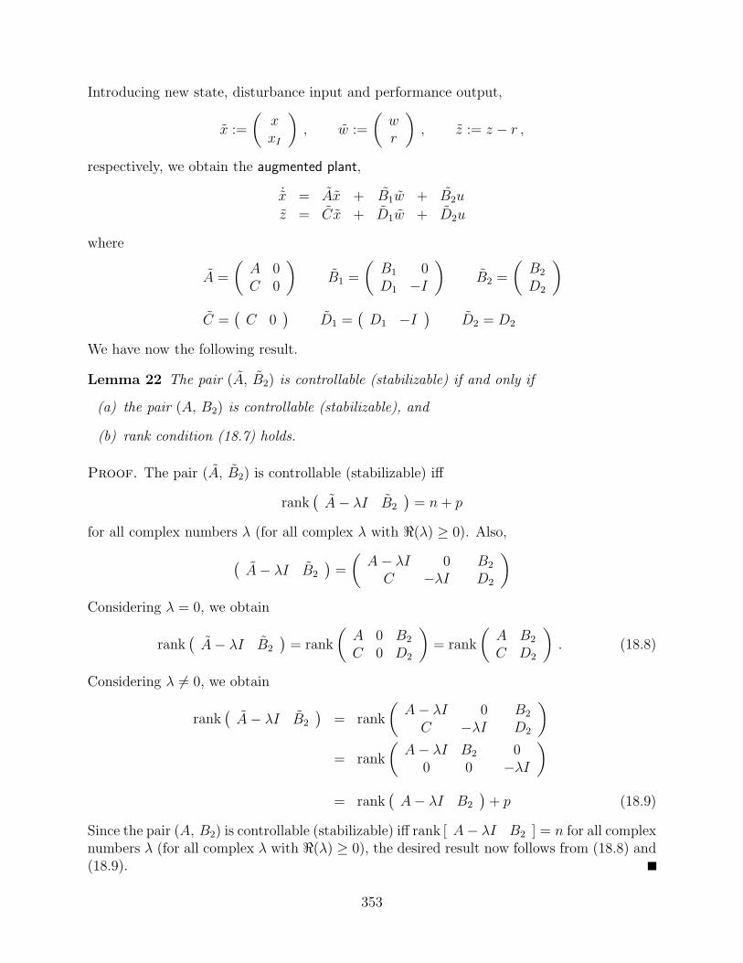
Introducing new state, disturbance input and performance output,

x :=

(xxI

), w :=

(wr

), z := z − r ,

respectively, we obtain the augmented plant,

˙x = Ax + B1w + B2u

z = Cx + D1w + D2u

where

A =

(A 0C 0

)B1 =

(B1 0D1 −I

)B2 =

(B2

D2

)

C =(

C 0)

D1 =(

D1 −I)

D2 = D2

We have now the following result.

Lemma 22 The pair (A, B2) is controllable (stabilizable) if and only if

(a) the pair (A, B2) is controllable (stabilizable), and

(b) rank condition (18.7) holds.

Proof. The pair (A, B2) is controllable (stabilizable) iff

rank(

A− λI B2

)= n + p

for all complex numbers λ (for all complex λ with <(λ) ≥ 0). Also,

(A− λI B2

)=

(A− λI 0 B2

C −λI D2

)

Considering λ = 0, we obtain

rank(

A− λI B2

)= rank

(A 0 B2

C 0 D2

)= rank

(A B2

C D2

). (18.8)

Considering λ 6= 0, we obtain

rank(

A− λI B2

)= rank

(A− λI 0 B2

C −λI D2

)

= rank

(A− λI B2 0

0 0 −λI

)

= rank(

A− λI B2

)+ p (18.9)

Since the pair (A, B2) is controllable (stabilizable) iff rank [ A− λI B2 ] = n for all complexnumbers λ (for all complex λ with <(λ) ≥ 0), the desired result now follows from (18.8) and(18.9).

353

Controller design. Suppose (A, B2) is stabilizable and rank condition (18.7) holds. Then(A, B2) is also stabilizable. Choose any matrix K such that A+B2K is asymptotically stable.Let

u = Kx

If we partition K asK =

(KP KI

)

where KP is given by the first n columns of K and KI is given by the last p columns of K,then the controller is given by

xI = z − ru = KP x + KIxI

Note that this controller can be written as

u = KP x + KI

∫(z − r)

This is a generalization of the classical PI (Proportional Integral) Controller.

Closed loop system. The closed loop system is given by

˙x = [A + B2K]x + B1w

z = [C + D2K]x + D1w

Since the matrix A + B2K is asymptotically stable and w is constant, all solutions x arebounded for t ≥ 0. Thus, x(t) is bounded for all t ≥ 0.

Letting η = ˙x and noting that w is constant, we obtain that

η = [A + B2K]η .

Since the matrix A + B2K is asymptotically stable, we must have

limt→∞

˙x = limt→∞

η(t) = 0 .

In particular, we havelimt→∞

xI = 0 ;

hencelimt→∞

z(t) = r .

Thus, the proposed controller achieves the desired behavior.

Example 206 Consider the constantly disturbed and controlled harmonic oscillator de-scribed by

x1 = x2

x2 = −x1 + w + u

z = x1

354

Here

A =

(0 1

−1 0

), B1 = B2 =

(01

), C =

(1 0

), D1 = D2 = 0

The pair (A, B2) is controllable and

rank

(A B2

C D2

)= rank

0 1 0−1 0 1

1 0 0

= 3 = n + p

Hence

A =

(A 0C 0

)=

0 1 0−1 0 0

1 0 0

, and B2 =

(B2

D2

)=

010

LettingK =

(k1 k2 kI

)

we obtain

A + B2K =

0 1 0−1 + k1 k2 kI

1 0 0

The characteristic polynomial p of A + B2K is given by

p(s) = s3 − k2s2 + (1− k1)s− kI

Choosing k1, k2, kI so that this polynomial has roots with negative real parts, a controlleryielding constant output tracking, rejecting constant disturbances and yielding boundedstates is given by

xI = x1 − ru = k1x1 + k2x2 + kIxI

18.3 Measured Output Feedback Control


x = Ax + B1w + B2uz = C1x + D11w + D12uy = C2x + D21w

where the n-vector x(t) is the state; the m1-vector w is an unknown, constant, disturbanceinput; the m2-vector u(t) is the control input; and the p1-vector z(t) is a performance output.We will assume z(t) can be measured and that instead of x we can only measure the measuredoutput y(t) which is a p2-vector.

Suppose the p1-vector r is any constant reference output and we wish to design a controllersuch that for any initial condition x(0) = x0,

limt→∞

z(t) = r

and the state x(t) is bounded for all t ≥ 0. To achieve this objective, we need the followingassumptions.

355

Assumptions.

(a) The pair (A, B2) is stabilizable.

(b) The pair (C2, A) is detectable.

(c)

rank

(A B2

C1 D12

)= n + p1

As before, we introduce a new state variable xI given by

xI = z − r

where xI(0) is arbitrary. Letting

x :=

(xxI

), w :=

(wr

), z := z − r , y :=

yxI

r

we obtain the augmented plant

˙x = Ax + B1w + B2u

z = C1x + D11w + D12u

y = C2x + D21w

(18.10)

with

A =

(A 0C1 0

)B1 =

(B1 0D11 −I

)B2 =

(B2

D12

)

C1 =(

C1 0)

D11 =(

D11 −I)

D12 = D12

C2 =

C2 00 I0 0

D21 =

D21 00 00 I

Consider now any output feedback controller of the form

xc = Acxc + Bcyu = Ccxc + Dcy

(18.11)

The resulting closed loop system is described by(

˙xxc

)=

(A + B2DcC2 B2Cc

BcC2 Ac

)

︸︷︷︸Acl

(xxc

)+

(B1 + B2DcD21

DcD21

)w (18.12)

From the lemma of the previous section, assumptions (a) and (c) imply that the pair (A, B2)is stabilizable. Also, detectability of the pair (C2, A) is equivalent to detectability of the pair(C2, A). Hence, one can always choose matrices Ac, Bc, Cc, Dc so that so that the closed loopsystem matrix Acl is asymptotically stable.

356

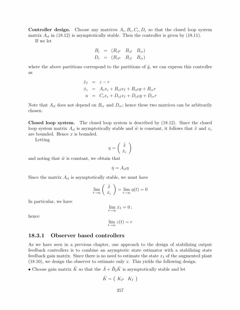
Controller design. Choose any matrices Ac, Bc, Cc, Dc so that the closed loop systemmatrix Acl in (18.12) is asymptotically stable. Then the controller is given by (18.11).

If we let

Bc = (BcP BcI Bcr)

Dc = (BcP BcI Bcr)

where the above partitions correspond to the partitions of y, we can express this controlleras

xI = z − r

xc = Acxc + BcIxI + BcP y + Bcrr

u = Ccxc + DcIxI + DcP y + Dcrr

Note that Acl does not depend on Bcr and Dcr; hence these two matrices can be arbitrarilychosen.

Closed loop system. The closed loop system is described by (18.12). Since the closedloop system matrix Acl is asymptotically stable and w is constant, it follows that x and xc

are bounded. Hence x is bounded.Letting

η =

(˙x

xc

)

and noting that w is constant, we obtain that

η = Aclη

Since the matrix Acl is asymptotically stable, we must have

limt→∞

(˙x

xc

)= lim

t→∞η(t) = 0

In particular, we havelimt→∞

xI = 0 ;

hencelimt→∞

z(t) = r

18.3.1 Observer based controllers

As we have seen in a previous chapter, one approach to the design of stabilizing outputfeedback controllers is to combine an asymptotic state estimator with a stabilizing statefeedback gain matrix. Since there is no need to estimate the state xI of the augmented plant(18.10), we design the observer to estimate only x. This yields the following design.

• Choose gain matrix K so that the A + B2K is asymptotically stable and let

K =(

KP KI

)

357

where KP is given by the first n columns of K and KI is given by the last p1 columns of K.

• Choose observer gain matrix L so that A + LC2 is asymptotically stable.

• An observer based controller is given by

xI = z − r integratorxc = Axc + B2u + L(C2xc − y) observeru = KP xc + KIxI control input

where xc(0) and xI(0) are arbitrary.

If we let

e := xc − x

the closed loop system due to this controller is described by

(˙xe

)=

(A + B2K ∗

0 A + LC2

)(xe

)+

( ∗∗

)w

Since the eigenvalues of the closed loop system matrix

(A + B2K ∗

0 A + LC2

)

are the union of those of A + B2K and A + LC2, it follows that this matrix is asympoticallystable. Hence, this controller yields the desired behavior.

Exercises


z(s) = Tzw(s)w(s) + Tzu(s)u(s)

with

Tzw(s) =1

s2 − 1and Tzu(s) =

s− 2

s2 − 1

where z, w, and u are the Laplace transforms of the performance output z, disturbanceinput w, and control input u, respectively. Let r be a desired constant output and assumethe disturbance input w is an unknown constant. Design an output (z) feedback controllerwhich guarantees that for all r and w,

limt→∞

z(t) = r

and all signals are bounded. Illustrate your results with simulations.

358


x = Ax + B1w + B2uy = Cx + D1w + D2u

where x(t), u(t), and w, and y(t) ∈ IRp are as above. Suppose that we can only measure thecontrol input u and the measured output y. It is desired to obtain an asymptotic observerfor x and w; that is, we wish to design an observer producing estimates x and w of x and wwith the property that for any initial value x0 of x and any w, one has

limt→∞

[x(t)− x(t)] = 0 , limt→∞

[w(t)− w] = 0

(a) State the least restrictive conditions on the system which allows one to construct anasymptotic estimator.

(b) Give a procedure for constructing an asymptotic estimator.

(c) Illustrate your results with example(s) and simulation results.

359

Chapter 19

Lyapunov revisited*

19.1 Stability, observability, and controllability

Recall the damped linear oscillator described by

x1 = x2

x2 = − km

x1 − dm

x2(19.1)

with m, d and k positive. This system is asymptotically stable. The energy of this system isgiven by

V (x) =k

2x2

1 +m

2x2

2 = x∗Px

where

P =

k2

0

0 m2

.

Along any solution, the rate of change of the energy is given by

dV

dt= −dx2

2 = −x∗C∗Cx

whereC =

[0 d

12

]

From this it should be clear that

P > 0

PA + A∗P + C∗C = 0

The matrix Q = C∗C is hermitian positive semi-definite, but it is not positive definite.Hence, using this P matrix, our existing Lyapunov results only guarantee that the system isstable; they do not guarantee asymptotic stability. Noting that the pair (C, A) is observable,we present a result in this section which allows us to use the above P matrix to guaranteeasymptotic stability of (19.1).

361


x = Ax (19.2)

where x(t) is an n-vector and A is a constant n× n matrix. We have the following result.

Lemma 23 Suppose there is a hermitian matrix P satisfying

P > 0PA + A∗P + C∗C ≤ 0

(19.3)

where (C,A) is observable. Then system (19.2) is asymptotically stable.

Proof. Suppose there exists a hermitian matrix P which satisfies inequalities (19.3). Con-sider any eigenvalue λ of A; we will show that <(λ) < 0. Let v 6= 0 be an eigenvectorcorresponding to λ, that is,

Av = λv . (19.4)

Hence,

v∗PAv = λv∗Pv ;

and taking the complex conjugate transpose of both sides of this last equation yields

v∗A∗Pv = λv∗Pv

Pre- and post-multiplying the second inequality in (19.3) by v∗ and v, respectively, yields

v∗PAv + v∗APv + v∗C∗Cv ≤ 0

which implies

λv∗Pv + λv∗Pv + ||Cv||2 ≤ 0

that is,

2<(λ)v∗Pv ≤ −||Cv||2 .

Since P > 0, we must have v∗Pv > 0.

We now show that we must also have ||Cv|| > 0. Suppose ||Cv|| = 0. Then Cv = 0.Recalling (19.4) results in [

A− λIC

]v = 0

Since (C,A) is observable, the above matrix has rank n, and hence v = 0; this contradictsv 6= 0. So, we must have ||Cv|| > 0.

Hence,

<(λ) = −||Cv||2/2v∗Pv < 0

Since <(λ) < 0 for every eigenvalue λ of A, system (19.2) is asymptotically stable.

362

Example 207 Returning to the damped linear oscillator, we see that inequalities (19.3) aresatisfied by

P =

[k2

00 m

2

]C =

[0 d

12

]

Since the oscillator is described by (19.2) with

A =

[0 1

− km

− dm

]

we have [C

CA

]=

[0 d

12

−d12 k

m−d

32

m

]

Since this observability matrix is invertible, (C,A) is observable. Using Lemma 23, one canuse the above matrix P to guarantee asymptotic stability of the damped oscillator.

Exercise 146 Prove the following result. Suppose there is a hermitian matrix P satisfying

P ≥ 0PA + A∗P + C∗C ≤ 0

where (C,A) is detectable. Then the system (19.2) is asymptotically stable.

Recalling that controllability of (A,B) is equivalent to observability of (B∗, A∗), and thatasymptotic stability of A and A∗ are equivalent, we obtain the following result

Lemma 24 Suppose there is a hermitian matrix S satisfying

S > 0AS + SA∗ + BB∗ ≤ 0

(19.5)

where (A,B) is controllable. Then system (19.2) is asymptotically stable

Exercise 147 Suppose there is a hermitian matrix S satisfying

S ≥ 0AS + SA∗ + BB∗ ≤ 0

where (A,B) is stabilizable. Then system (19.2) is asymptotically stable

Suppose system (19.2) is asymptotically stable, Then for any matrix C (of appropriatedimensions) the Lyapunov equation

PA + A∗P + C∗C = 0 (19.6)

has the unique solution

P =

∫ ∞

0

eA∗tC∗CeAt dt

Recall that this is the infinite time observability grammian associated with (C, A), that is,P = Wo; it is always hermitian and positive semidefinite. In addition, as we have seenearlier, Wo is positive definite if and only if (C,A) is observable. These observations andLemma 23 lead to the following result.

363



(b) There exist a positive definite hermitian matrix P and a matrix C with (C, A) observ-able which satisfy the Lyapunov equation

PA + A∗P + C∗C = 0 (19.7)

(c) For every matrix C with (C, A) observable, the Lyapunov equation (19.7) has a uniquesolution for P and this solution is hermitian positive-definite.

Recall the original Lyapunov equation

PA + A∗P + Q = 0

If Q is hermitian positive semi-definite, it can always be expressed as Q = C∗C by appropriatechoice of C and one can readily show that (Q,A) is observable iff (C,A) is observable. AlsorankC = n if and only if Q is positive definite. If C has rank n, the pair (C, A) is observablefor any A. So, if Q is positive definite hermitian, the original Lyapunov equation is of theform (19.7) with (C,A) observable.

Recalling that controllability of (A,B) is equivalent to observability of (B∗, A∗), and thatasymptotic stability of A and A∗ are equivalent, we can obtain the following result.



(b) There exist a positive definite hermitian matrix S and a matrix B with (A, B) control-lable which satisfy the Lyapunov equation

AS + SA∗ + BB∗ = 0 (19.8)

(c) For every matrix B with (A, B) controllable, the Lyapunov equation (19.8) has a uniquesolution for S and this solution is hermitian positive-definite.

Note that if A is asymptotically stable, the solution S to Lyapunov equation (19.8) isthe infinite-time controllability grammian associated with (A,B), that is S = Wc. Also,

S =

∫ ∞

0

eAtBB∗eA∗t dt

364

19.2 A simple stabilizing controller

Consider a linear time-invariant system described by

x = Ax + Bu

where x(t) is an n-vector and u(t) is an m-vector. Consider any positive T > 0 and let

W = Wc(−T ) :=

∫ 0

−T

eAtBB∗eA∗t dt

The above matrix can be regarded as the finite time controllability grammian (over theinterval [−T, 0]) associated with (A,B). If (A, B) is controllable, W is invertible.

We now show that the controller

u = −B∗W−1x

yields an asymptotically stable closed loop system.

Using the following properties of eAt,

AeAt =deAt

dt; eA∗tA∗ =

deA∗t

dt

we obtain

AW + WA∗ =

∫ 0

−T

[AeAtBB∗eA∗t + eAtBB∗eA∗tA∗] dt

=

∫ 0

−T

[deAt

dtBB∗eA∗t + eAtBB∗deA∗t

dt

]dt

=

∫ 0

−T

d(eAtBB∗eA∗t

)

dtdt

= BB∗ − e−AT BB∗e−A∗T ,

that is,AW + WA∗ −BB∗ = −e−AT BB∗e−A∗T

Considering the closed loop system

x = (A−BB∗W−1)x

we have

(A−BB∗W−1)W + W (A−BB∗W−1)∗ = AW + WA∗ − 2BB∗

= −BB∗ − e−AT BB∗e−A∗T

≤ −BB∗ ,

365

that is,(A−BB∗W−1)W + W (A−BB∗W−1)∗ + BB∗ ≤ 0 .

Controllability of (A, B) implies controllability of (A − BB∗W−1, B). This fact, alongwith W > 0 and the previous inequality imply that the closed-loop system is asymptoticallystable.

So, the above yields another proof of

controllability =⇒ stabilizability

366

Chapter 20

Performance*

20.1 The L2 norm

20.1.1 The rms value of a signal

Consider any scalar signal s which is defined for 0 ≤ t < ∞. One measure of the size of thesignal is given by the rms value of the signal; we denote this by ‖s‖2 and define it by

‖s‖2 =

(∫ ∞

0

|s(t)|2 dt

) 12

.

This is also called the L2 norm of the signal. One can readily show that the three requiredproperties of a norm are satisfied. This norm is simply the generalization of the usualEuclidean norm for n-vectors to signals or functions. Clearly, a signal has a finite L2 normif and only if it is square integrable.

Example 208 Consider the exponential signal s(t) = eλt where λ = −α + jω and α and ωare both real with α > 0. For any T > 0,

∫ T

0

|s(t)|2 dt =

∫ T

0

e−2αt dt =1

−2α(e−2αT − 1) .

Thus, ∫ ∞

0

|s(t)|2 dt = limT→∞

∫ T

0

|s(t)|2 dt = limT→∞

1

−2α(e−2αT − 1) =

1

2α.

Hence ‖s‖2 = 1/√

2α.

Consider now a signal s where s(t) is an n-vector for 0 ≤ t < ∞. We define the L2 normof the signal s by

‖s‖2 =

(∫ ∞

0

|s(t)|2 dt

) 12

where ‖s(t)‖ is the usual Euclidean norm of the n-vector s(t) as given by

‖s(t)‖2 = |s1(t)|2 + |s2(t)|2 + · · ·+ |sn(t)|2 .

One can readily show that the three required properties of a norm are satisfied.

367

20.1.2 The L2 norm of a time-varying matrix

Consider now a function G defined on [0,∞) where G(t) is a matrix for 0 ≤ t < ∞. Wedefine the L2 norm of G by

‖G‖2 =

(∫ ∞

0

trace (G∗(t)G(t)) dt

) 12

.

Suppose G(t) is m×n and the m-vectors g1(t), g2(t), · · · , gn(t) are the columns of G(t). Then

trace (G(t)∗G(t)) = g1(t)∗g1(t) + g2(t)

∗g2(t) + · · ·+ gn(t)∗gn(t)

= ‖g1(t)‖2 + ‖g2(t)‖2 + · · ·+ ‖gn(t)‖2 .

So we conclude that

‖G‖22 =

n∑i=1

∫ ∞

0

‖gi(t)2‖2 dt =

n∑i=1

‖gi‖22 (20.1)

where the gi is the i-th column of G.

20.2 The H2 norm of an LTI system

Consider an input-output system with disturbance input w and performance output z de-scribed by

x = Ax + Bwz = Cx

(20.2)

and suppose A is asymptotically stable. Recall that zero initial condition input-outputbehavior of this system can be completely characterized by its impulse response

G(t) = CeAtB . (20.3)

Consider first a SISO system with impulse response g. When A is asymptotically stable,it follows that g is square integrable and the L2 norm ‖g‖2 of g is finite where

‖g‖2 =

(∫ ∞

0

|g(t)|2 dt

) 12

. (20.4)

We refer to ‖g‖2 as the H2 norm of the system. Thus the H2 norm of an asymptotically stableSISO system is the rms value of its impulse response. This norm is a a performance measurefor the system; it can be regarded as a measure of the ability of the system to mitigate theeffect of the disturbance w on the performance output z.

Consider now a general linear time-invariant system described by (20.2) with inpulseresponse given by (20.3). When A is asymptotically stable, if follows that each element ofG is square integrable, and we define the L2 norm of the impulse response by

‖G‖2 =

(∫ ∞

0

trace (G∗(t)G(t)) dt

) 12

. (20.5)

368

We refer to ‖G‖2 as the H2 norm of the system.We now obtain a frequency domain interpretation of ‖G‖2. Recall that the transfer

function of this system is given by G(s) = C(sI −A)−1B. When A is asymptotically stable,we define the 2-norm of the transfer function by

‖G‖2 =

(1

2π

∫ ∞

−∞trace (G(ω)∗G(ω)) dω

) 12

. (20.6)

For a SISO system with transfer function g, we have

‖g‖22 =

1

2π

∫ ∞

−∞|g(ω)|2 dω .

Since G is the Laplace transform of G, it follows from Parseval’s Theorem that

‖G‖2 = ‖G‖2 , (20.7)

that is, the 2-norm of the transfer function equals the L2 norm of the impulse response.

20.3 Computation of the H2 norm

We now show how the H2-norm can be computed using Lyapunov equations. Suppose A isasymptotically stable and let Wo be the observability grammian associated with (C, A), thatis, Wo =

∫∞0

eA∗tC∗CeAt dt. Recall that Wo is the unique solution to the Lyapunov equation

WoA + A∗Wo + C∗C = 0 .

We now obtain that∫ ∞

0

G∗(t)G(t) dt =

∫ ∞

0

B∗eA∗tC∗CeAtB dt = B∗∫ ∞

0

eA∗tC∗CeAt dtB = B∗WoB ,

that is, ∫ ∞

0

G∗(t)G(t) dt = B∗WoB . (20.8)

Using the linearity of the trace operation, it now follows that

‖G(·)‖22 =

∫ ∞

0

trace (G∗(t)G(t)) dt = trace

(∫ ∞

0

G∗(t)G(t) dt

)= trace (B∗WoB) ;

hence

‖G‖22 = trace (B∗WoB) . (20.9)

We can also compute the H2-norm using the controllability grammian. Since

trace (G∗(t)G(t)) = trace (G(t)G∗(t)) ;

369

it follows that the H2-norm is also given by

‖G‖2 =

(∫ ∞

0

trace (G(t)G∗(t)) dt

) 12

. (20.10)

Let Wc be the controllability grammian associated with (A,B), that is, Wo =∫∞0

eAtBB∗eA∗t dt.Recall that Wc is the unique solution to the Lyapunov equation

AWc + WcA∗ + BB∗ = 0 .

Hence,∫ ∞

0

G(t)G(t)∗ dt =

∫ ∞

0

CeAtBB∗eA∗tC∗ dt = C

∫ ∞

0

eAtBB∗eA∗t dtC∗ = CWcC∗ ,

that is, ∫ ∞

0

G(t)G∗(t) dt = CWcC∗ . (20.11)

Using the linearity of the trace operation, it now follows that

‖G(·)‖22 =

∫ ∞

0

trace (G(t)G∗(t)) dt = trace

(∫ ∞

0

G(t)G∗(t) dt

)= trace (CWcC

∗) ;

hence‖G‖2

2 = trace (CWcC∗) . (20.12)

Example 209 Consider the scalar system described by

x = −αx + u

y = x

with α > 0. This system has transfer function g(s) = 1s+α

. Hence,

‖g‖22 =

1

2π

∫ ∞

−∞|g|2 dω =

1

2π

∫ ∞

−∞

1

α2 + ω2dω =

1

2πα

∫ ∞

−∞

1

1 + η2dη (η = ω/α)

=1

2πα

∣∣∞−∞ tan−1(η)

=1

2α.

The impulse response for this system is given by g(t) = e−αt. Hence

‖g‖22 =

∫ ∞

0

g(t)2 dt =

∫ ∞

0

e−2αt dt = |∞01

−2αe−2αt

=1

2α.

This clearly illustrates the fact that ‖g‖2 = ‖g‖2 and the H2 norm of this system is (1/2α)12 .

370

The observability grammian Wo is given by the solution to the Lyapunov equation

−Woα− αWo + 1 = 0 .

This yields Wo = 1/2α. Since B = 1, we readily see that the H2 norm is given by

trace (B∗WoB)12 . The controllability grammian Wc is given by the solution to the Lyapunov

equation−αWc −Wcα + 1 = 0 .

This yields Wc = 1/2α. Since C = 1, we readily see that the H2 norm is given by

trace (CWcC∗)

12 .

MATLAB

>> help normh2

NORMH2 Continuous H2 norm.

[NMH2] = NORMH2(A,B,C,D) or

[NMH2] = NORMH2(SS_) computes the H2 norm of the given state-space

realization. If the system not strictly proper, INF is returned.

Otherwise, the H2 norm is computed as

NMH2 = trace[CPC’]^0.5 = trace[B’QB]^0.5

where P is the controllability grammian, and Q is the observability

grammian.

>> help norm2

nh2 = norm2(sys)

Computes the H2 norm of a stable and strictly proper LTI

system

-1

SYS = C (sE-A) B

This norm is given by

______________

/

V Trace(C*P*C’)

where P solves the Lyapunov equation: A*P+P*A’+B*B’ = 0.

See also LTISYS.

371

Exercises


x1 = x2

x2 = −2x1 − 3x2 + w

y = 4x1 + 2x2

Obtain the H2 norm of this system using the following methods.(a) The definition in (20.4).(b) Equation (20.9).(c) Equation (20.11).(d) MATLAB.

Exercise 149 Without carrying out any integration, obtain the H2 norm of the systemwhose impulse response g is given by

g(t) = e−t + e−2t .

372

Chapter 21

Linear quadratic regulators (LQR)

21.1 The linear quadratic optimal control problem

In this chapter we learn another method of designing stabilizing state feedback controllers.These controllers result from solving the linear quadratic (LQ) optimal control problem andare called linear quadratic regulators (LQR). This problem is characterized by a linear systemand a quadratic cost.

Consider a linear time-invariant system (plant)

x = Ax + Bu (21.1)

with initial condition

x(0) = x0 (21.2)

where the real scalar t is the time variable, the n-vector x(t) is the plant state, and them-vector u(t) is the control input. When we refer to a control history, control signal, oropen loop control we will mean a continuous control input function u(·) which is defined for0 ≤ t < ∞.

Suppose Q and R are hermitian matrices with

R > 0 and Q ≥ 0

We call them weighting matrices. For each initial state x0 and each control history u(·), wedefine the corresponding quadratic cost by

J(x0, u(·)) :=

∫ ∞

0

x(t)∗Qx(t) + u(t)∗Ru(t) dt

where x(·) is the unique solution of (21.1) with initial condition (21.2). We wish to minimizethis cost by appropriate choice of the control history. Although the above cost can be infinite,it follows from the assumptions on Q and R that it is always non-negative, that is,

0 ≤ J(x0, u(·)) ≤ ∞ .

373

In addition to minimizing the above cost, we will demand that the control input drivesthe state to zero, that is, we require that

limt→∞

x(t) = 0 .

So, for a fixed initial state x0, we say that a control history u(·) is admissible at x0 if it resultsin limt→∞ x(t) = 0. We say that a control history uopt(·) is optimal at x0 if it is admissibleat x0 and

J(x0, uopt(·)) ≤ J(x0, u(·)) (21.3)

for every admissible control history u(·). We refer to

Jopt(x0) := J(x0, uopt(·))

as the optimal cost at x0.In general, the optimal control history and the optimal cost depend on the initial state.

Also, for a fixed initial state, the optimal cost is unique whereas the optimal control historyneed not be. In some cases an optimal control history might not exist. Since the cost isbounded below by zero, there is always an infimal cost J inf (x0). That is, one cannot achievebetter than this cost but can come arbitrarily close to it; more precisely, for every admissiblecontrol history u(·), one has

J inf (x0) ≤ J(x0, u(·))and for every ε > 0 there is an admissible control history uε(·) such that

J(x0, uε(·)) ≤ J inf (x0) + ε

When an optimal control history exists, we must have J inf (x0) = Jopt(x0). If there exists atleast one admissible control history yielding a bounded cost, then J inf (x0) < ∞.

Example 210 Consider the scalar integrator plant described by

x = u

with initial condition x(0) = 1. Suppose we wish to drive the state of this plant to zero whileminimizing the cost ∫ ∞

0

u(t)2 dt .

Consider any positive δ > 0 and let

u(t) = −δe−δt .

Then, the resulting state history, x(t) = e−δt, has the desired behavior and the correspondingcost is ∫ ∞

0

δ2e−2δt dt = |∞0δ

−2e−2δt =

δ

2.

By choosing δ > 0 arbitrarily small, we can make the cost arbitrarily close to zero. Sincethe cost is bounded below by zero, it follows that the infimal cost is zero. However, wecannot make the cost zero. If the cost is zero, that is

∫∞0

u(t)2 dt = 0, then we must haveu(t) ≡ 0; hence x(t) ≡ 1. This control history does not drive the state to zero and, hence,is not admissible. So there is no optimal control history for this problem. Note that in thisproblem, (Q,A) = (0, 0) has an imaginary axis unobservable eigenvalue.

374

Optimal feedback controllers. Suppose one has a feedback controller C with the prop-erty that for any initial state x0 the control histories generated by the controller are admissi-ble. We say that C is an optimal feedback controller if for each initial state x0 the correspondingcontrol histories generated by C are optimal at x0. We will shortly demonstrate the followingfact for linear quadratic optimal control problems:

If there is an optimal control history for every initial state then, for every initial state, theoptimal control history is unique and is given by a linear memoryless state feedback controller.

Since we are going to look controllers which minimize the cost and result in

limt→∞

x(t) = 0

we need to make the following assumption for the rest of the chapter:

• The pair (A,B) is stabilizable.

21.2 The algebraic Riccati equation (ARE)

We will see that, when an optimal feedback controller exists, its determination involves thefollowing matrix equation which is known as the Algebraic Riccati Equation (ARE):

PA + A∗P − PBR−1B∗P + Q = 0 (21.4)

The matrices A,B,Q, R are determined by the LQR problem data. Solving the LQR probleminvolves solving the ARE for a hermitian matrix P . Since the ARE depends quadraticallyon P , it is a nonlinear matrix equation and, in general, has more than one solution.

A solution P is said to be a stabilizing solution if the matrix A − BR−1B∗P is Hurwitz,that is, all its eigenvalues have negative real parts. This is the solution we will be lookingfor. The significance of this property is that the linear state feedback controller

u = −R−1B∗Px

results in the asymptotically stable closed loop system:

x = (A−BR−1B∗P )x

It shown in Section 21.4 that if there is an optimal control history for every initial statethen, the ARE must have a stabilizing solution. Hence, if the ARE does not have a stabilizingsolution then, there is not an optimal control history for every initial state.

It is also shown in Section 21.4 that if the pair (Q,A) has no imaginary unobservableeigenvalues then, the ARE must have a stabilizing solution.

Section 21.4 also shows that a stabilizing solution is maximal in the sense that if P is astabilizing and P is any other solution then, P ≥ P . Hence there can only be one stabilizingsolution.

375

21.3 Linear state feedback controllers

Supposeu(t) = Kx(t)

where K is a constant state feedback gain matrix. The resulting closed loop system isdescribed by

x = (A + BK)x

and for each initial state x0 the controller results in the cost

J(x0, u(·)) = J(x0, K) :=

∫ ∞

0

x(t)∗[K∗RK + Q]x(t) dt

This feedback controller is an optimal feedback controller if and only if it is a stabilizingcontroller (that is, A + BK is asymptotically stable) and for each initial state x0 we have

J(x0, K) ≤ J(x0, u(·))for every admissible control history u(·).

If K is stabilizing then, recalling a result from Lyapunov theory,

J(x0, K) = x∗0Px0 (21.5)

where P is the unique solution to the following Lyapunov equation

P (A + BK) + (A + BK)∗P + K∗RK + Q = 0 (21.6)

Since A + BK is asymptotically stable and K∗RK + Q is hermitian positive semi-definite,we have P ∗ = P ≥ 0.

Example 211 Consider the simple real scalar system

x = αx + u

with cost ∫ ∞

0

u(t)2 dt

If we do not require limt→∞ x(t) = 0 then regardless of initial state x0, this cost is uniquelyminimized by

u(t) ≡ 0

and the resulting controlled system is described by

x = αx

This system is not asymptotically stable for α ≥ 0. So, in looking for an optimal control werestrict consideration to control inputs that result in limt→∞ x(t) = 0

Now consider any linear controller u = kx. This generates a closed loop system

x = (α + k)x

376

which is asymptotically stable if and only if α + k < 0. Utilizing (21.5), (21.6), the costcorresponding to a stabilizing linear controller is Px2

0 where

P =k2

−2(α + k)

If α = 0, P = −k/2. Since we require asymptotic stability of the closed loop system, thiscost can be made arbitrarily small but nonzero. So for α = 0, we have an infimum cost (thatis, zero) but no minimum cost. The infimum cannot be achieved by controls which drivethe state to zero. Note that in this case, (Q, A) = (0, 0) has an imaginary axis unobservableeigenvalue.

21.4 Infimal cost*

21.4.1 Reduced cost stabilizing controllers.

Suppose one has a stabilizing gain matrix K and wishes to obtain another stabilizing gainmatrix which results in reduced cost. We will show that this is achieved by the gain matrix

K = −R−1B∗P (21.7)

where P solves the Lyapunov equation (21.6).

Fact 13 Suppose A + BK is asymptotically stable and K is given by (21.7) and (21.6).Then,

(i) the matrix A + BK is asymptotically stable;

(ii) for every initial state x0,J(x0, K) ≤ J(x0, K)

Proof. The Appendix contains a proof.

21.4.2 Cost reducing algorithm

The above result suggests the following algorithm to iteratively reduce the cost.

Jack Benny algorithm.

(0) Choose any gain matrix K0 so that A + BK0 is asymptotically stable.

(1) For k = 0, 1, 2, · · · , let Pk be the unique solution to the Lyapunov equation

Pk(A + BKk) + (A + BKk)∗Pk + K∗

kRKk + Q = 0 (21.8)

and letKk+1 = −R−1B∗Pk (21.9)

377

Fact 14 Suppose (A,B) is stabilizable, R∗ = R > 0 and Q∗ = Q ≥ 0. Consider anysequence of matrices Pk generated by the Jack Benny algorithm. Then this sequence has alimit P , that is,

limk→∞

Pk = P .

Furthermore, P has the following properties.

(a)P ∗ = P ≥ 0

(b) P = P solves

PA + A∗P − PBR−1B∗P + Q = 0 (21.10)

(c) Every eigenvalue of the matrix A−BR−1B∗P has real part less than or equal to zero.

(d) If (Q,A) has no imaginary axis unobservable eigenvalues, then every eigenvalue of thematrix A−BR−1B∗P has negative real part.

Proof. (a) Since Pk solves (21.8) we have Pk ≥ 0. From consequence (ii) of fact 13, wehave that Pk+1 ≤ Pk. Hence,

0 ≤ Pk+1 ≤ Pk

From this one can show that there is a matrix P such that

P := limk→∞

Pk

and P ≥ 0.(b) In the limit, and using (21.9),

K := limk→∞

Kk = limk→∞

Kk+1 = −R−1B∗P

hence, it follows from (21.8) that

P (A + BK) + (A + BK)∗P + K∗RK + Q = 0 (21.11)

SubstitutingK = −R−1B∗P

results in (21.10).(c) For each k, <(λ) < 0 for all eigenvalues λ of A + BK. Since K = limk→∞ Kk and

the eigenvalues of a matrix depend continuously on its coefficients, we must have <(λ) ≤ 0for all eigenvalues λ of A + BK.

(d) Now suppose A+BK has an eigenvalue λ with <(λ) = 0. Letting v be an eigenvector0 to λ and pre- and post-multiplying (21.11) by v∗ and v yields

v∗K∗RKv + v∗Qv = 0

378

Hence,Kv = 0 Qv = 0

andλv = (A + BK)v = Av

So, (A− λI

Q

)v = 0

that is, λ is an unobservable eigenvalue of (Q,A). So, if (Q,A) has no imaginary axisunobservable eigenvalues, A + BK has no imaginary axis eigenvalues. So all the eigenvaluesof A + BK have negative real parts.

Example 212 Recall first example. Here the algorithm yields:

Pk =K2

k

−2(α + Kk)

Kk+1 = −Pk

Hence,

Pk+1 =P 2

k

2(−α + Pk)

1. (α < 0): Here P = limk→∞ Pk = 0 and A−BR−1B∗P = α < 0.

2. (α > 0): Here P = limk→∞ Pk = 2α and A−BR−1B∗P = −α < 0.

3. (α = 0): Here Pk+1 = Pk/2 for all k. Hence, P = limk→∞ Pk = 0 andA−BR−1B∗P = 0.

Note that this is the only case in which (Q,A) has an imaginary axis unobservableeigenvalue.

Remark 11 The matrix equation (21.10) is called an algebraic Riccati equation (ARE). Sinceit depends quadratically on P , it is a nonlinear matrix equation and, in general, has morethan one solution.

Remark 12 We say that a hermitian matrix P is a stabilizing solution to ARE (21.10) if allthe eigenvalues of the matrix A − BR−1B∗P have negative real parts. The significance ofthis is that the controller

u = −R−1B∗Px

results in the asymptotically stable closed loop system:

x = (A−BR−1B∗P )x

379

21.4.3 Infimal cost

The following result provides a lower bound on the infimal cost J inf (x0) in terms of a specificsolution to the ARE.

Fact 15 (Completion of squares lemma.) Suppose R∗ = R > 0 and P is any hermitiansolution to ARE (21.10). Then for every initial condition x0 and every continuous controlinput history u(·) which guarantees

limt→∞

x(t) = 0

we havex∗0Px0 ≤ J(x0, u(·)) ;

hencex∗0Px0 ≤ J inf (x0) .

Proof. Suppose P is any hermitian solution P to the ARE (21.10), let x0 be any initialstate, and consider any control history u(·) which results in limt→∞ x(t) = 0. Consider thefunction V (x(·)) given by

V (x(t)) = x∗(t)Px(t)

Its derivative is given by

dV (x(t))

dt= 2x∗(t)Px(t)

= 2x∗(t)PAx + 2x∗(t)PBu(t)

Utilizing the ARE (21.10) we obtain

2x∗PAx = x∗(PA + A∗P )x

= x∗PBR−1B∗Px− x∗Qx

Hence (omitting the argument t for clarity),

dV (x(t))

dt= x∗PBR−1B∗Px + 2x∗PBu− x∗Qx

= x∗PBR−1B∗Px + 2x∗PBu + u∗Ru− x∗Qx− u∗Ru

= (u + R−1B∗Px)∗R(u + R−1B∗Px)− x∗Qx− u∗Ru

Hence

x∗Qx + u∗Ru = −dV (x)

dt+ (u + R−1B∗Px)∗R(u + R−1B∗Px)

Considering any t ≥ 0 and integrating over the interval [0, t] yields

∫ t

0

(x∗Qx + u∗Ru) dt = −V (x(t)) + V (x(0)) +

∫ t

0

(u + R−1B∗Px)∗R(u + R−1B∗Px) dt

380

Recall V (x) = x∗Px, x(0) = x0, and limt→∞ x(t) = 0; so, considering the limit as t →∞and recalling the definition of the cost, we have

J(x0, u(·)) = x∗0Px0 +

∫ ∞

0

(u + R−1B∗Px)∗R(u + R−1B∗Px) dt (21.12)

Since R > 0, we immediately have

J(x0, u(·)) ≥ x∗0Px0 (21.13)

The next result states that for any initial state x0, the infimal cost is x∗0P x0 where P isthe limit of any sequence Pk generated by Jack Benny algorithm.

Lemma 25 (Infimal cost lemma.) Suppose (A,B) is stabilizable, R∗ = R > 0 and Q∗ = Q ≥0. Consider any sequence of matrices Pk∞k=0 generated by the Jack Benny algorithm. Thenthis sequence has a limit P , that is,

limk→∞

Pk = P

and P has the following properties.

(a) If P is any hermitian solution to ARE (21.10), then

P ≥ P

(b) For every initial state x0,

J inf (x0) = x∗0P x0

(c) If there exists an optimal control history for every initial state x0 then P is a stabilizingsolution to ARE (21.10).

Proof. Consider any sequence of matrices Pk generated by the Jack Benny algorithm.Then, from fact (14), this sequence has a limit P , that is,

limk→∞

Pk = P

and it satisfies ARE (21.10).Consider any initial state x0 and any k = 1, 2, . . . . The control history given by

uk(t) = −R−1B∗Pk−1x(t)

results in the costJ(x0, uk(·)) = x∗0Pkx0

HenceJ inf(x0) ≤ x∗0Pkx0

381

Since P is a solution to the ARE, it follows from the completion of squares lemma that

x∗0P x0 ≤ J inf(x0)

Hencex∗0P x0 ≤ J inf(x0) ≤ x∗0Pkx0

Considering the limit as k →∞ we must have

x∗0P x0 ≤ J inf(x0) ≤ x∗0P x0 ;

soJ inf (x0) = x∗0P x0

If P is any hermitian solution to ARE (21.10), we must have

x∗0Px0 ≤ J(x0, uk(·)) = x∗0Pkx0

Taking the limit as k →∞, we obtain

x∗0Px0 ≤ x∗0P x0

Since this is true for all x0 we have P ≤ P .Suppose an optimal control history uopt exists for every x0. Then

J(x0, uopt) = Jopt(x0) = J inf(x0) = x∗0P x0

Recalling the proof of the completion of squares lemma, we have

J(x0, uopt(·)) = x∗0P x0 +

∫ ∞

0

(uopt + R−1B∗P x)∗R(uopt + R−1B∗P x) dt

Hence ∫ ∞

0

(uopt + R−1B∗P x)∗R(uopt + R−1B∗P x) dt = 0

Since R > 0 we must haveuopt = −R−1B∗P x

Since uopt(·) is admissable, it results in limt→∞. Since the above is true for any initial statex0, it follows that the system

x = (A−BR−1B∗)x

must be asymptotically stable. Hence P is a stabilizing solution to ARE.

Remark 13 A solution to the ARE which satisfies condition (a) above is called the maximalsolution to the ARE. Clearly, it must be unique.

382

21.5 Optimal stabilizing controllers

The solution to the LQR problem is based on the following matrix equation which is knownas the Algebraic Riccati Equation:

PA + A∗P − PBR−1B∗P + Q = 0 (21.14)

Since this is a nonlinear equation in P it can have more that one solution. We will beinterested in a stabilizing solution which is defined as a hermitian matrix P with the propertythat all the eigenvalues of the matrix A−BR−1B∗P have negative real parts.

Theorem 32 Suppose R∗ = R > 0 and the ARE (21.14) has a stabilizing solution P . Thenfor every initial state x0, there is a unique optimal control history uopt; it is given by

uopt(t) = −R−1B∗Px(t)

and the optimal cost isJopt(x0) = x∗0Px0 .

Proof. Let x0 be any initial state, and consider any control history u(·) which results inlimt→∞ x(t) = 0. Define the function V given by

V (t) = x∗(t)Px(t)

The derivative of V is given by

dV

dt= 2x∗(t)Px(t)

= 2x∗(t)PAx(t) + 2x∗(t)PBu(t)

Utilizing the ARE (21.14) we obtain

2x∗PAx = x∗(PA + A∗P )x

= x∗PBR−1B∗Px− x∗Qx

Hence (omitting the argument t for clarity),

dV

dt= x∗PBR−1B∗Px + 2x∗PBu− x∗Qx

= x∗PBR−1B∗Px + 2x∗PBu + u∗Ru− x∗Qx− u∗Ru

= (u + R−1B∗Px)∗R(u + R−1B∗Px)− x∗Qx− u∗Ru

Hence

x∗Qx + u∗Ru = −dV

dt+ (u + R−1B∗Px)∗R(u + R−1B∗Px)

383

Considering any t ≥ 0 and integrating over the interval [0, t] yields

∫ t

0

(x∗Qx + u∗Ru) dt = −V (t) + V (0) +

∫ t

0

(u + R−1B∗Px)∗R(u + R−1B∗Px) dt

Recall V (t) = x∗(t)Px(t), x(0) = x0, and limt→∞ x(t) = 0; so, considering the limit ast →∞ and recalling the definition of the cost, we have

J(x0, u(·)) = x∗0Px0 +

∫ ∞

0

(u + R−1B∗Px)∗R(u + R−1B∗Px) dt (21.15)

Since P is a stabilizing solution to ARE (21.10) the control history given by u(t) =u(t) := −R−1B∗Px(t) results in limt→∞ x(t) = 0; hence

J(x0, u(·)) = x∗0Px0

Consider any other admissible control history u(·). Since R > 0, we have

J(x0, u(·)) ≥ x∗0Px0

This implies that u is optimal at x0 and the optimal cost is x∗0Px0.Also, (21.15) implies that if any other control u yields the optimal cost x∗0Px0, then the

u(t) = −R−1B∗Px(t); hence u(t) = u(t). So, u is a unique optimal control history.

Example 213 Returning to Example 211 we have A = α, B = 1, Q = 0, and R = 1. Hencethe ARE is

2αP − P 2 = 0

This has two solutionsP = P1 := 0 P = P2 := 2α

HenceA−BR−1B∗P1 = α A−BR−1B∗P2 = −α

We have three cases.Case 1. (α < 0): P1 = 0 is the stabilizing solution and optimal controller is u = 0.Case 2. (α > 0): P1 = 2α is the stabilizing solution and optimal controller is u = −2αx.Case 3. (α = 0): No stabilizing solution.

Remark 14 If P is a stabilizing solution to ARE (21.10) then, it can be shown that P mustbe the maximal solution P . This follows from

x∗0Px0 = Jopt(x0) = J inf(x0) = x∗0P x0 .

Hence there can be at most one stabilizing solution.

384

21.5.1 Existence of stabilizing solutions to the ARE

Lemma 26 Suppose (A, B) is stabilizable, R∗ = R > 0 and Q∗ = Q. Then ARE (21.10) hasa stabilizing solution if and only if (Q,A) has no imaginary axis unobservable eigenvalues.

Proof. From Fact 14 it follows that if (Q,A) has no imaginary unobservable eigenvaluesthen the ARE has a stabilizing solution.

We now prove the converse by contradiction. Suppose P is a stabilizing solution to AREand λ is an imaginary unobservable eigenvalue of (Q,A). Then, there is a nonzero vector vsuch that

Av = λv and Qv = 0

Pre- and postmultiplying the ARE by v∗ and v yields

2<(λ)v∗Pv − v∗PBR−1B∗Pv = 0

Hence, R−1B∗Pv = 0 and

(A−BR−1B∗P )v = Av −BR−1B∗Pv

= λv

that is, λ is an eigenvalue of the matrix A − BR−1B∗P . This contradicts the asymptoticstability of this matrix.

Lemma 27 Suppose (A,B) is stabilizable, R∗ = R > 0 and Q∗ = Q ≥ 0. If (Q,A) isdetectable, then

(a) The ARE has a stabilizing solution.

(b) P is a stabilizing solution if and only if P ≥ 0

Proof. Part (a) follows from previous lemma.(b) We have already seen that if P is stabilizing then P ≥ 0. So, all we have to show is

that if P solves the ARE and P ≥ 0 then P must be stabilizing. To prove this we write theARE as

P (A + BK) + (A + BK)∗P + K∗RK + Q = 0

where K = −R−1B∗P . Hence,

P (A + BK) + (A + BK)∗P + Q ≤ 0

Since P ≥ 0 and (Q,A) is detectable, it follows from a previous Lyapunov result that A+BKis asymptotically stable; hence P is stabilizing.

385

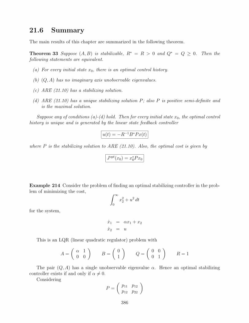
21.6 Summary

The main results of this chapter are summarized in the following theorem.

Theorem 33 Suppose (A,B) is stabilizable, R∗ = R > 0 and Q∗ = Q ≥ 0. Then thefollowing statements are equivalent.

(a) For every initial state x0, there is an optimal control history.

(b) (Q,A) has no imaginary axis unobservable eigenvalues.

(c) ARE (21.10) has a stabilizing solution.

(d) ARE (21.10) has a unique stabilizing solution P ; also P is positive semi-definite andis the maximal solution.

Suppose any of conditions (a)-(d) hold. Then for every initial state x0, the optimal controlhistory is unique and is generated by the linear state feedback controller

u(t) = −R−1B∗Px(t)

where P is the stabilizing solution to ARE (21.10). Also, the optimal cost is given by

Jopt(x0) = x∗0Px0

Example 214 Consider the problem of finding an optimal stabilizing controller in the prob-lem of minimizing the cost, ∫ ∞

0

x22 + u2 dt

for the system,

x1 = αx1 + x2

x2 = u

This is an LQR (linear quadratic regulator) problem with

A =

(α 10 0

)B =

(01

)Q =

(0 00 1

)R = 1

The pair (Q,A) has a single unobservable eigenvalue α. Hence an optimal stabilizingcontroller exists if and only if α 6= 0.

Considering

P =

(p11 p12

p12 p22

)

386

(we are looking for a symmetric P ) the ARE yields the following three scalar equations

2αp11 − p212 = 0

p11 + αp12 − p12p22 = 02p12 − p2

22 + 1 = 0(21.16)

We consider three cases:

Case 1 (α < 0.) The first equation in (21.16) yields p11 = p212/α. Since we require p11 ≥ 0

we must have

p11 = p12 = 0

The second equation in (21.16) is now automatically satisfied and (requiring p22 ≥ 0) thethird equation yields

p22 = 1

Since

P =

(0 00 1

)

is the only positive semi-definite solution to the ARE; it must be the stabilizing one. Thefact that it is stabilizing is evident from

Acl = A−BR−1B∗P =

(α 10 −1

)

So, the optimal stabilizing controller for this case is given by

u = −x2

Case 2 (α > 0.) We obtain three positive semi-definite solutions:

Pi =

(β2

i /2α βi

βi (1 + 2βi)12

)β1 = 2α(α + 1), β2 = 2α(α− 1), β3 = 0

Since (P1)11 ≥ (P2)11, (P3)11, and the stabilizing solution is maximal, the matrix P1 mustbe the stabilizing solution. Let us check that P1 is indeed a stabilizing solution. Thecorresponding closed loop matrix,

Acl = A−BR−1B∗P1 =

(α 1

−β1 −(1 + 2β1)12

)

has characteristic polynomial

q(s) = s2 + a1s + a0

witha1 = (1 + 2β1)

12 − α = (4α2 + 4α + 1)

12 − α > 0

a0 = β1 − α(1 + 2β1)12 = 2α(α + 1)− α(4α2 + 4α + 1)

12 > 0

387

Since all coefficients of this second order polynomial are positive, all roots of this polynomialhave negative real part; hence Acl is asymptotically stable. So, the optimal stabilizingcontroller for this case is given by

u = −2α(α + 1)x1 − (4α2 + 4α + 1)12 x2

Case 3 (α = 0.) We already know that there is no optimal stabilizing controller for this case.However, to see this explicitly note that the only positive semi-definite solution to the AREis

P =

(0 00 1

)

Since

Acl = A−BR−1B∗P =

(0 10 −1

),

this solution is not stabilizing; hence there there is no stabilizing solution and no optimalstabilizing controller.

388

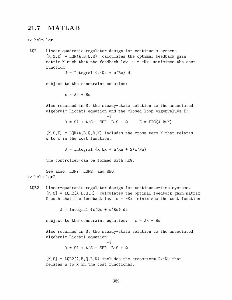
21.7 MATLAB

>> help lqr

LQR Linear quadratic regulator design for continuous systems.

[K,S,E] = LQR(A,B,Q,R) calculates the optimal feedback gain

matrix K such that the feedback law u = -Kx minimizes the cost

function:

J = Integral x’Qx + u’Ru dt

subject to the constraint equation:

.

x = Ax + Bu

Also returned is S, the steady-state solution to the associated

algebraic Riccati equation and the closed loop eigenvalues E:

-1

0 = SA + A’S - SBR B’S + Q E = EIG(A-B*K)

[K,S,E] = LQR(A,B,Q,R,N) includes the cross-term N that relates

u to x in the cost function.

J = Integral x’Qx + u’Ru + 2*x’Nu

The controller can be formed with REG.

See also: LQRY, LQR2, and REG.

>> help lqr2

LQR2 Linear-quadratic regulator design for continuous-time systems.

[K,S] = LQR2(A,B,Q,R) calculates the optimal feedback gain matrix

K such that the feedback law u = -Kx minimizes the cost function

J = Integral x’Qx + u’Ru dt

.

subject to the constraint equation: x = Ax + Bu

Also returned is S, the steady-state solution to the associated

algebraic Riccati equation:

-1

0 = SA + A’S - SBR B’S + Q

[K,S] = LQR2(A,B,Q,R,N) includes the cross-term 2x’Nu that

relates u to x in the cost functional.

389

The controller can be formed with REG.

LQR2 uses the SCHUR algorithm of [1] and is more numerically

reliable than LQR, which uses eigenvector decomposition.

See also: ARE, LQR, and LQE2.

>> help are

ARE Algebraic Riccati Equation solution.

X = ARE(A, B, C) returns the stablizing solution (if it

exists) to the continuous-time Riccati equation:

A’*X + X*A - X*B*X + C = 0

assuming B is symmetric and nonnegative definite and C is

symmetric.

See also: RIC.

21.8 Minimum energy controllers

Suppose we are interested in stabilizing a system with the minimum amount of control effort.Then, we might consider the problem of minimizing

∫ ∞

0

‖u(t)‖2 dt

subject to

x = Ax + Bu and x(0) = x0 and limt→∞

x(t) = 0 . (21.17)

This is an LQR problem with Q = 0 and R = I. The corresponding ARE is

PA + A∗P − PBR−1B∗P = 0 . (21.18)

Since Q = 0, it follows from our main LQR result that that an optimal stabilizing controllerexists if and only if A has no imaginary eigenvalues.

The optimal controllers for this problem result in a closed loop system having the followinginteresting property.

If λ is an eigenvalue of A := A + BK = A − BR−1B∗P , then either λ or −λ is aneigenvalue of A.

To demonstrate the above property, rewrite ARE as

PA + A∗P = 0 .

390

Suppose λ is an eigenvalue of A. Then there is a nonzero vector v such that Av = λv.Post-multiplying the ARE by v yields

λPv + A∗Pv = 0

If Pv 6= 0, then Pv is an eigenvector of A∗ with eigenvalue −λ. Hence , −λ is an eigenvalueof A. If Pv = 0, then Av = Av−BB∗Pv = Av; hence Av = λv and λ is an eigenvalue of A.

Example 215 Suppose we wish to obtain a stabilizing state feedback controller which al-ways minimizes

∫∞0

u(t)2 dt for the scalar system

x = ax + u .

HereA = a , B = 1 , R = 1 , Q = 0 .

So the problem has a solution provided a is not on the imaginary axis. The ARE corre-sponding to this problem,

(a + a)P − P 2 = 0 ,

has two solutionsP = 0 and P = a + a .

The two corresponding values of A := A−BR−1B∗P are

a and − a

respectively.From this we can explicitly that, when a is on the imaginary axis, there is no stabilizing

P .When a has negative real part, P = 0 is stabilizing, the optimal controller is zero and

A = A.When a has positive real part, P = a + a is stabilizing, the optimal controller is u =

−(a + a)x and A = −a.

391

21.9 H2 optimal controllers*


x = Ax + B1w + B2u

z = Cx + Du

where the m1-vector w(t) is a disturbance input; the m2-vector u(t) is a control input; andthe p-vector z performance output. We assume that

(i) rankD = m2.

(ii) D∗C = 0.

With the above assumptions, the energy ‖z‖2 associated with the output is given by

‖z‖22 =

∫ ∞

0

‖z(t)‖2 dt =

∫ ∞

0

‖Cx(t) + Du(t)‖2 dt =

∫ ∞

0

(x(t)∗Qx(t) + u(t)∗Ru(t)) dt

withQ = C∗C and R = D∗D .

Since D has full column rank, it follows that R is positive definite.A linear state feedback controller

u = Kx

results in the closed loop system

x = (A + B2K)x + B1w (21.19a)

z = (C + DK)x (21.19b)

Suppose that A + B2K is asymptotically stable and recall the definition of the H2-norm ofa linear system. If GK is the impulse response matrix from w to z then the H2 norm of the

above system is given by ‖GK‖2 =(trace

(∫∞0

G∗K(t)GK(t) dt

)) 12 . Noting that

(C + DK)∗(C + DK) = C∗C + K∗D∗DK

it follows that‖GK‖2

2 = traceB∗1PKB1

where PK is the unique solution to

PK(A + B2K) + (A + B2K)∗PK + K∗D∗DK + C∗C = 0 .

From this one can readily show that if one considers the LQ problem with

B = B2 , R = D∗D , Q = C∗C

then an optimal LQ controller minimizes the H2 norm of the closed loop system.The observability condition on (Q,A) is equivalent to:

392

• The pair (C, A) has no imaginary axis unobservable eigenvalues.

So provided this condition holds the controller which minimizes ‖GK‖2 is given by

u = −(D∗D)−1B∗2P

where P is the stabilizing solution to

PA + A∗P − PB∗1(D

∗D)−1B∗1P + C∗C = 0

• If A+B2K is asymptotically stable, it follows from an identity in Lyapunov revisited that

‖GK‖22 = trace (C + DK)∗X(C + DK)

where X is the unique solution to

(A + B2K)X + X(A + B2K)∗ + B∗1B1 = 0

The hermitian positive semi-definite matrix X is sometimes referred to as the state covariancematrix associated with the above system.

393

21.10 Exercises


x = 2x + u ,

where x and u are real scalars. Obtain an optimal stabilizing feedback controller which mini-mizes ∫ ∞

0

u(t)2 dt .


x1 = −x1 + x2

x2 = x2 + u ,

where x1, x2 and u are real scalars. Obtain an optimal stabilizing feedback controller whichminimizes ∫ ∞

0

u(t)2 dt .


x1 = −x2 + u

x2 = −x1 − u

where all quantities are scalar. Obtain a optimal stabilizing feedback controller which mini-mizes ∫ ∞

0

u(t)2 dt .

Exercise 153 For the system

x1 = αx1 + x2

x2 = −x2 + u

Obtain a optimal feedback controller which minimizes∫ ∞

0

u(t)2 dt

You may have to distinguish between different cases of α.

Exercise 154 2-link manipulator Recall the two link manipulator with measured outputy = q2. Recall the linearization of this system about

q1 = q2 = u = 0

and recall its state space description.Obtain an LQG controller for this linearized system. Apply the controller to the nonlinear

system and simulate the nonlinear closed loop system for various initial conditions. (Use zeroinitial conditions for the observer.)

394

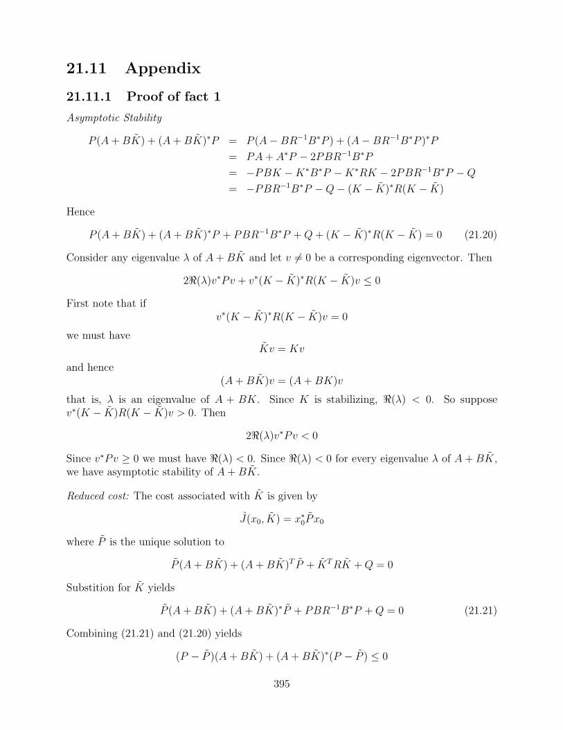
21.11 Appendix

21.11.1 Proof of fact 1

Asymptotic Stability

P (A + BK) + (A + BK)∗P = P (A−BR−1B∗P ) + (A−BR−1B∗P )∗P

= PA + A∗P − 2PBR−1B∗P

= −PBK −K∗B∗P −K∗RK − 2PBR−1B∗P −Q

= −PBR−1B∗P −Q− (K − K)∗R(K − K)

Hence

P (A + BK) + (A + BK)∗P + PBR−1B∗P + Q + (K − K)∗R(K − K) = 0 (21.20)

Consider any eigenvalue λ of A + BK and let v 6= 0 be a corresponding eigenvector. Then

2<(λ)v∗Pv + v∗(K − K)∗R(K − K)v ≤ 0

First note that ifv∗(K − K)∗R(K − K)v = 0

we must haveKv = Kv

and hence(A + BK)v = (A + BK)v

that is, λ is an eigenvalue of A + BK. Since K is stabilizing, <(λ) < 0. So supposev∗(K − K)R(K − K)v > 0. Then

2<(λ)v∗Pv < 0

Since v∗Pv ≥ 0 we must have <(λ) < 0. Since <(λ) < 0 for every eigenvalue λ of A + BK,we have asymptotic stability of A + BK.

Reduced cost: The cost associated with K is given by

J(x0, K) = x∗0P x0

where P is the unique solution to

P (A + BK) + (A + BK)T P + KT RK + Q = 0

Substition for K yields

P (A + BK) + (A + BK)∗P + PBR−1B∗P + Q = 0 (21.21)

Combining (21.21) and (21.20) yields

(P − P )(A + BK) + (A + BK)∗(P − P ) ≤ 0

395

In other words, for some hermitian positive semi-definite matrix ∆Q,

(P − P )(A + BK) + (A + BK)∗(P − P ) + ∆Q = 0

Since A + BK is asymptotically stable,

P − P =

∫ ∞

0

e(A+BK)∗t∆Qe(A+BK)t dt

Hence P − P ≥ 0, orP ≤ P

396

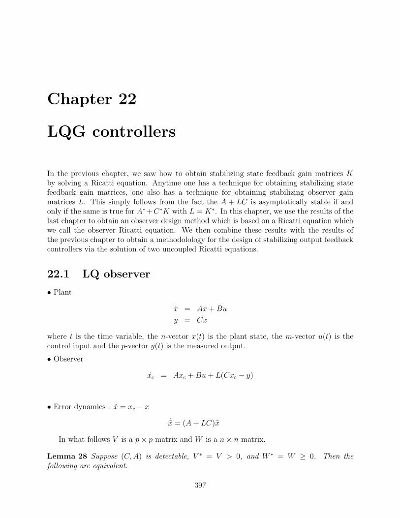
Chapter 22

LQG controllers

In the previous chapter, we saw how to obtain stabilizing state feedback gain matrices Kby solving a Ricatti equation. Anytime one has a technique for obtaining stabilizing statefeedback gain matrices, one also has a technique for obtaining stabilizing observer gainmatrices L. This simply follows from the fact the A + LC is asymptotically stable if andonly if the same is true for A∗+C∗K with L = K∗. In this chapter, we use the results of thelast chapter to obtain an observer design method which is based on a Ricatti equation whichwe call the observer Ricatti equation. We then combine these results with the results ofthe previous chapter to obtain a methodolology for the design of stabilizing output feedbackcontrollers via the solution of two uncoupled Ricatti equations.

22.1 LQ observer

• Plant

x = Ax + Bu

y = Cx

where t is the time variable, the n-vector x(t) is the plant state, the m-vector u(t) is thecontrol input and the p-vector y(t) is the measured output.

• Observer

xc = Axc + Bu + L(Cxc − y)

• Error dynamics : x = xc − x

˙x = (A + LC)x

In what follows V is a p× p matrix and W is a n× n matrix.

Lemma 28 Suppose (C, A) is detectable, V ∗ = V > 0, and W ∗ = W ≥ 0. Then thefollowing are equivalent.

397

(i) The pair (A,W ) has no imaginary axis uncontrollable eigenvalues.

(ii) The Riccati equation

AS + SA∗ − SC∗V −1CS + W = 0 (22.1)

has a hermitian solution S with A− SC∗V −1C asymptotically stable.

Proof. By duality.

• We will refer to ARE (22.1) as an observer Riccati equation associated with the plant.

• We say that S is a stabilizing solution to (22.1) if A − SC∗V −1C is asymptotically stable.The significance of this is that if one chooses the observer gain L as

L = −SC∗V −1 (22.2)

then the error dynamics are described by the asymptotically stable system

˙x = (A− SC∗V −1C)x

22.2 LQG controllers

Plant

x = Ax + Buy = Cx

Basically we combine an LQR regulator with an LQ observer.

So suppose the the plant satisfies the following minimal requirements for stabilization viaoutput feedback:

(i) (A,B) is stabilizable.

(ii) (C,A) is detectable.

Choose weighting matricesQ R W V

(of appropriate dimensions) which satisfy the following conditions:

(i) R∗ = R > 0 and Q∗ = Q ≥ 0, and (Q, A) has no imaginary axis unobservableeigenvalues.

(ii) V ∗ = V > 0 and W ∗ = W ≥ 0, and (A,W ) has no imaginary axis uncontrollableeigenvalues.

Let P and S be the stabilizing solutions to the Riccati equations

PA + A∗P − PBR−1B∗P + Q = 0

AS + SA∗ − SC∗V −1CS + W = 0

398

LQG Controller The corresponding LQG controller is given by

xc = (A−BR−1B∗P )xc − SC∗V −1(Cxc − y)u = −R−1B∗Pxc

Note that this can be written as

xc = (A−BR−1B∗P − SC∗V −1C)xc + SC∗V −1y

u = −R−1B∗Pxc

Letting ˙x = xc − x, the closed loop system is described by

x = (A−BR−1B∗P )x − BR−1B∗Px˙x = (A− SC∗V −1C)x

As we have seen before the eigenvalues of this closed loop system are simply the union ofthose of the asymptotically matrices A− BR−1B∗P and A− SC∗V −1C. Hence, the closedloop system is asymptotically stable.

22.3 H2 Optimal controllers*

22.3.1 LQ observers

Consider

x = Ax + B1w + B2u

y = Cx + Dw

where the measurement vector y(t) is a p-vector. We assume that

(i) rankD = p

(ii) DB∗1 = 0

With an observerxc = Axc + B2u + L(Cxc − y) ,

the corresponding observer error dynamics are described by

˙x = (A + LC)x + (B1 − LD)w .

Note that(B1 − LD)(B1 − LD)∗ = B1B

∗1 + LDD∗L∗

Consider any “performance variable”

z = Mx

399

Suppose A + LC is asymptotically stable and GL is the impulse response matrix from w toz. Then, the H2 norm of GL is given by

‖GL‖22 =

∫ ∞

0

trace (G∗(t)G(t)) dt = MSLM∗

where SL uniquely solves

(A + LC)SL + SL(A + LC)∗ + LDD∗L∗ + B1B∗1 = 0

WithV = DD∗ W = B1B

∗1

the corresponding LQ observer minimizes the H2 norm of GL.The controllability condition on (A,W ) is equivalent to:

• The pair (A,B1) has no imaginary axis uncontrollable eigenvalues.

So provided this condition holds the observer gain which minimizes the H2 norm of GL

is given byL = −SC∗(DD∗)−1

where S is the stabilizing solution to

AS + SA∗ − SC∗(DD∗)−1CS + B1B∗1 = 0

22.3.2 LQG controllers

Considerx = Ax + B1w + B2uz = C1x + D12uy = C2x + D21w

400

Chapter 23

Systems with inputs and outputs: II*

Recall

←− x = Ax + Buy = Cx + Du

←− (23.1)

23.1 Minimal realizations

Recall that (A,B, C, D) is a realization of a transfer matrix G if

G(s) = C(sI − A)−1B + D.

• A realization is minimal if the dimension of its state-space is less than or equal to the statespace dimension of any other realization.

SISO systems. Consider a SISO system described by

G(s) =n(s)

d(s)

where n and d are polynomials. If n and d are coprime (i.e., they have no common zeros),then the order of a minimal realization is simply the degree of d.

Equivalent systems. System


is equivalent to system˙x = Ax + Bu

y = Cx + Du

if there is a nonsingular matrix T such that

A = T−1AT B = T−1B

C = CT D = D

401

Theorem 34

(i) (A,B, C,D) is a minimal realization of G(s) iff (A,B) is controllable and (C, A) isobservable.

(ii) All minimal realizations are equivalent.

23.2 Exercises


G(s) =

1

s− 1

1

s− 1

1

s + 1− 1

s + 1

.



G(s) =

[s

s− 1

1

s + 1

].


Problem 2 Obtain a minimal state space realization of the transfer function

G(s) =s2 − 3s + 2

s2 + s− 2.

402

Chapter 24

Time-varying systems*

24.1 Linear time-varying systems (LTVs)

Here we are concerned with linear time-varying systems (LTVs) systems described by

x(t) = A(t)x(t) + B(t)u(t)y(t) = C(t)x(t) + D(t)u(t)

(24.1)

where t is the time variable, the state x(t) is an n-vector, the input u(t) is an m-vector whilethe output y(t) is a p-vector. We suppose that the time-varying matrices A(t), B(t), C(t), D(t)depend continuously on t.

24.1.1 Linearization about time-varying trajectories

Consider a nonlinear system described by

x = F (x, u) (24.2a)

y = H(x, u) . (24.2b)

Suppose u(·) is a specific time-varying input history to the nonlinear system and x(·) is anycorresponding state trajectory. Then

˙x(t) = F (x(t), u(t)) .

Let y(·) be the corresponding output history, that is,

y(t) = F (y(t), u(t)) .

Then, introducing the perturbed variables

δx = x− x and δu = u− u and δy = y − y ,

the linearization of system (24.2) about (x, u) is defined by

δx = A(t)δx + B(t)δu (24.3a)

δy = C(t)δx + D(t)δu (24.3b)

403

where

A(t) =∂F

∂x(x(t), u(t)) and B(t) =

∂F

∂x(u(t), u(t))

C(t) =∂H

∂x(x(t), u(t)) and D(t) =

∂H

∂u(x(t), u(t)) .

Note that, although the original nonlinear system is time-invariant, its linearization about atime-varying trajectory can be time-varying.

24.2 The state transition matrix

Consider a linear time-varying system described by

x = A(t)x (24.4)

where t is the time variable, x(t) is an n-vector and the time-varying matrix A(t) dependscontinuously on t.

Fact 16 We have existence and uniqueness of solutions, that is, for each initial condition,

x(t0) = x0 , (24.5)

there is a unique solution to the differential equation (24.4) which satisfies the initial condi-tion. Also, this solution is defined for all time.

Fact 17 Solutions depend linearly on initial state. More specifically, for each pair of timest, t0, there is a matrix Φ(t, t0) such that for every initial state x0, the solution x(t) at time tdue to initial condition (24.5) is given by

x(t) = Φ(t, t0)x0

The matrix Φ(t, t0) is called the state transition matrix associated with system (24.4).Note that it is uniquely defined by

Φ(t0, t0) = I

∂Φ

∂t(t, t0) = A(t)Φ(t, t0)

LTI systems

x = Ax

Φ(t, t0) = eA(t−t0)

404

Scalar systems. Consider any scalar system described by

x = a(t)x

where x(t) and a(t) are scalars. The solution to this system corresponding to initial conditionx(t0) = x0 is given by

x(t) = e∫ t

t0a(τ) dτ

x0 .

Hence,

Φ(t, t0) = e∫ t

t0a(τ) dτ

Some properties of the state transition matrix

(a)

Φ(t2, t1)Φ(t1, t0) = Φ(t2, t0)

(b) Φ(t, t0) is invertible and

Φ(t0, t) = Φ(t, t0)−1

(c)∂Φ

∂t0(t, t0) = −Φ(t, t0)A(t0)

(d)

det[Φ(t, t0)] = exp

∫ t

t0

trace [A(τ)] dτ

Computation of the state transition matrix. Let X be the solution of

X(t) = A(t)X(t) (24.6a)

X(0) = I (24.6b)

where I is the n×n identity matrix. Then X(t) = Φ(t, 0). Hence, using property (b) above,X(t0)

−1 = Φ(0, t0) Now use property (a) to obtain

Φ(t, t0) = X(t)X(t0)−1 (24.7)

24.3 Stability

Recall that when A is a constant matrix, system (24.4) is asymptotically stable if and onlyif all the eigenvalues of A have negative real parts. This leads to the following naturalconjecture: system (24.4) is asymptotically stable if the eigenvalues of A(t) have negativereal parts for all time t. This conjecture is, in general, false. This is demonstrated by thefollowing example. Actually, in this example, the eigenvalues of A(t) are the same for all tand have negative real parts. However, the system has unbounded solutions and is unstable.

405

Example 216 (Markus and Yamabe, 1960.) This is an example of an unstable secondorder system whose time-varying A matrix has constant eigenvalues with negative real parts.Consider

A(t) =

[ −1 + a cos2 t 1− a sin t cos t−1− a sin t cos t −1 + a sin2 t

]

with 1 < a < 2. Here,

Φ(t, 0) =

[e(a−1)t cos t e−t sin t−e(a−1)t sin t e−t cos t

]

Since a > 1, the system corresponding to this A(t) matrix has unbounded solutions. However,for all t, the characteristic polynomial of A(t) is given by

p(s) = s2 + (2− a)s + 2

Since 2− a > 0, the eigenvalues of A(t) have negative real parts.

24.4 Systems with inputs and outputs

x = A(t)x + B(t)u x(t0) = x0 (24.8)

y = C(t)x + D(t)u (24.9)

• The solution to (24.8) is uniquely given by

x(t) = Φ(t, t0)x0 +

∫ t

t0

Φ(t, τ)B(τ)u(τ) dτ

Impulse response matrix

y(t) = C(t)Φ(t, t0)x0 +

∫ t

t0

C(t)Φ(t, τ)B(τ)u(τ) dt + D(t)u(t)

Hence, for x(t0) = 0,

y(t) =

∫ t

t0

G(t, τ)u(τ) dτ

whereG(t, τ) := C(t)Φ(t, τ)B(τ) + D(τ)δ(τ)

24.5 DT

x(k) = Φ(k, k0)︸︷︷︸state transition matrix

x0

406

Fact 18 (a)Φ(k0, k0) = I

(b)Φ(k2, k1)Φ(k1, k0) = Φ(k2, k0)

(c)Φ(k + 1, k0) = A(k)Φ(k, k0)

LTIΦ(k) = Ak

407

Chapter 25

Appendix A: Complex stuff

25.1 Complex numbers

Think about ordered pairs (α, β) of real numbers α, β and suppose we define addition oper-ation and a multiplication operation by

(α, β) + (γ, δ) = (α + γ, β + δ)

(α, β)(γ, δ) = (αγ − βδ, αδ + βγ)

respectively. It can readily be shown that these two operations satisfy the ‘usual’ rules ofaddition and multiplication for real numbers.

Consider now any two ordered pairs of the form (α, 0) and (γ, 0). Using the abovedefinitions of addition and multiplication we obtain

(α, 0) + (γ, 0) = (α + γ, 0)

and(α, 0)(β, 0) = (αβ, 0)

(check it out) So we can identify each ordered pair of the form (α, 0) with the real numberα and the above definitions of addition and multiplication reduce to the usual ones for realnumbers.

Now consider := (0, 1). Using the above definition of multiplication, we obtain

j2 = (0, 1)(0, 1) = (−1, 0)

In other words (identifying (−1, 0) with the real number −1),

j2 = −1

We also note that for any real number β,

jβ = (0, 1)(β, 0) = (0, β)

409

hence,

(α, β) = (α, 0) + (0, β) = α + jβ

If we regard the set C of complex numbers as the set of ordered pairs of real numbersfor which an addition and multiplication are as defined above, we arrive at the followingrepresentation of complex nubers.

• A complex number λ can be written as

λ = α + β

where α, β are real numbers and j2 = −1. The real numbers α and β are called the real partand imaginary part of λ and are denoted by

α := <(λ) β := =(λ)

respectively.Note

(α + jβ) + (γ + jδ) = α + γ + j(β + δ)

and

(α + jβ)(γ + jδ) = αγ + jαδ + jβγ + j2βδ

= (αγ − βδ) + j(αδ + βγ)

In other words, we recovered our original definitions of complex addition and multiplication.

• If λ = α + β, its complex conjugate λ is defined by

λ := α− β

Some properties:

<(λ) =1

2(λ + λ)

=(λ) =1

2j(λ− λ)

λ + η = λ + η

λη = λη

• The absolute value of λ:

|λ| =√

λλ

=√

α2 + β2

410

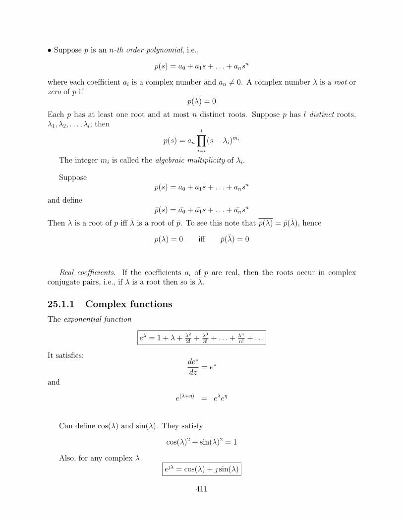
• Suppose p is an n-th order polynomial, i.e.,

p(s) = a0 + a1s + . . . + ansn

where each coefficient ai is a complex number and an 6= 0. A complex number λ is a root orzero of p if

p(λ) = 0

Each p has at least one root and at most n distinct roots. Suppose p has l distinct roots,λ1, λ2, . . . , λl; then

p(s) = an

l∏i=i

(s− λi)mi

The integer mi is called the algebraic multiplicity of λi.

Supposep(s) = a0 + a1s + . . . + ansn

and definep(s) = a0 + a1s + . . . + ansn

Then λ is a root of p iff λ is a root of p. To see this note that p(λ) = p(λ), hence

p(λ) = 0 iff p(λ) = 0

Real coefficients. If the coefficients ai of p are real, then the roots occur in complexconjugate pairs, i.e., if λ is a root then so is λ.

25.1.1 Complex functions

The exponential function

eλ = 1 + λ + λ2

2!+ λ3

3!+ . . . + λn

n!+ . . .

It satisfies:dez

dz= ez

and

e(λ+η) = eλeη

Can define cos(λ) and sin(λ). They satisfy

cos(λ)2 + sin(λ)2 = 1

Also, for any complex λ

eλ = cos(λ) + sin(λ)

411

Hence, for any real number β,

eβ = cos(β) + sin(β)

and|eβ| =

√cos(β)2 + sin(β)2 = 1

Also,e(α+β) = eαeβ = eα cos β + eα sin β

Hence,|e(α+β)| = |eα| |eβ)| = eα

25.2 Complex vectors and Cn

Read all the material on real vectors and replace the word real with the word complex andIR with C.

If x ∈ Cn, the complex conjugate of x:

x :=

x1

x2...

xn

Some properties:

x + y = x + y

λx = λx

<(x) =1

2(x + x)

=(x) =1

2j(x− x)

25.3 Complex matrices and Cm×n

Read all the material on real matrices and replace the word real with the word complex andIR with C

If A ∈ Cm×n, the complex conjugate of A:

A :=

a11 a12 . . . a1n

a21 a22 . . . a2n...

......

am1 am2 . . . amn

412

Some properties:

A + B = A + B

λA = λA

AB = AB

<(A) =1

2(A + A)

=(A) =1

2j(A− A)

The complex conjugate transpose of A:

A∗ := AT

=

a11 a21 . . . am1

a12 a22 . . . am2...

......

a1n a2n . . . amn

Some properties:

(A + B)∗ = A∗ + B∗

(λA)∗ = λA∗

(AB)∗ = B∗A∗

DEFN. A is hermitian ifA∗ = A

413

Chapter 26

Appendix B: Norms

26.1 The Euclidean norm

What is the size or magnitude of a vector? Meet norm.

• Consider any complex n vector x.The Euclidean norm or 2-norm of x is the nonegative real number given by

||x|| := (|x1|2 + . . . + |xn|2) 12

Note that

||x|| = (x1x1 + . . . + xnxn)12

= (x∗x)12

If x is real, these expressions become

||x|| = (x21 + . . . + x2

n)12

= (xT x)12

>> norm([3; 4])

ans = 5

>> norm([1; j])

ans = 1.4142

Note that in the last example xT x = 0, but x∗x = 2.

Properties of || · ||. The Euclidean norm has the following properties.

415

(i) For every vector x,||x|| ≥ 0

and||x|| = 0 iff x = 0

(ii) (Triangle Inequality.) For every pair of fectors x, y,

||x + y|| ≤ ||x||+ ||y||

(iii) For every vector x and every scalar λ.

||λx|| = |λ|||x||

Any real valued function on a vector space which has the above three properties is definedto be a norm. Two other commonly encountered norms on the space of n-vectors are the1-norm:

‖x‖1 := |x1|+ . . . + |xn|and the ∞-norm:

‖x‖∞ := maxi|xi|

As a example of a norm on the set of m× n matrices A, consider

‖A‖ = Tr(A′A)12 =

(m∑

i=1

n∑j=1

|Aij|2) 1

2

where Tr(M) denotes the trace of a square matrix M , that is the sum of its diagonal elements.This norm is called the Frobenius norm and is the matrix analog of the Euclidean norm forn-vectors. We will meet other matrix norms later.

416

Chapter 27

Appendix C: Some linear algebra

All the definitions and results of this section are stated for real scalars. However, they alsohold for complex scalars; to get the results for complex scalars, simply replace ‘real’ with‘complex’ and IR with C.

27.1 Linear equations

Many problems in linear algebra can be reduced to that of solving a bunch of linear equa-tions in a bunch of unknowns. Consider the following m linear scalar equations in n scalarunknowns x1, x2, . . . , xn:

a11x1 + a12x2 + · · ·+ a1nxn = b1

a21x1 + a22x2 + · · ·+ a2nxn = b2...

am1x1 + am2x2 + · · ·+ amnxn = bm

(27.1)

Given the scalars aij and bi, a basic problem is that of determining whether or not theabove system of linear equations has a solution for x1, x2, · · · , xn and, if a solution exists,determining all solutions.

One approach to solving the above problem is to carry out a sequence of elementaryoperations on the above equations to reduce them to a much simpler system of equationswhich have the same solutions as the original system. There are three elementary operations:

1) Interchanging two equations.

2) Multiplication of an equation by a nonzero scalar.

3) Addition of a multiple of one equation to another different equation.

Each of the above operations are reversible and do not change the set of solutions.

The above approach is usually implemented by expressing the above equations in matrixform and carrying out the above elementary operations via elementary matrix row operations.

417

Introducing

b =

b1

b2...

bm

, A =

a11 a12 · · · a1n

a21 a22 · · · a2n...

......

am1 am2 · · · amn

and x =

x1

x2...

xn

,

the above system of scalar equations can written in matrix form as:

Ax = b (27.2)

where x is an n-vector, b is an m-vector and A is an m× n matrix.

Elementary row operations. The above elementary operations on the original scalarequations are respectively equivalent to the following elementary row operations on the aug-mented matrix: (

A b)

associated with the scalar equations.

1) Interchanging two rows.2) Multiplication of a row by a nonzero scalar.3) Addition of a multiple of one row to another different row.

The reduced row echelon form of a matrix. Consider any matrix M . For each non-zero row, the leading element of that row is the first non-zero element of the row. Thematrix M is said to be in reduced row echelon form if its structure satisfies the following fourconditions.

1) All zero rows come after the nonzero rows.2) All leading elements are equal to one.3) The leading elements have a staircase pattern.4) If a column contains a leading element of some row, then all other elements of the columnare zero.

This is illustrated with the following matrix.

M =

0 · · · 0 1 ∗ · · · 0 ∗ · · · 0 · · · ∗0 · · · 0 0 0 · · · 1 ∗ · · · 0 · · · ∗0 · · · 0 0 0 · · · 0 0 · · · 1 · · · ∗...

......

......

......

...0 · · · 0 0 0 · · · 0 0 · · · 0 · · · 00 · · · 0 0 0 · · · 0 0 · · · 0 · · · 0

(27.3)

So, the matrices

0 1 0 0 2

0 0 1 0 3

0 0 0 1 4

1 2 0 0 2

0 0 1 0 3

0 0 0 1 4

1 0 0 2 0

0 0 1 3 0

0 0 0 0 10 0 0 0 0

418

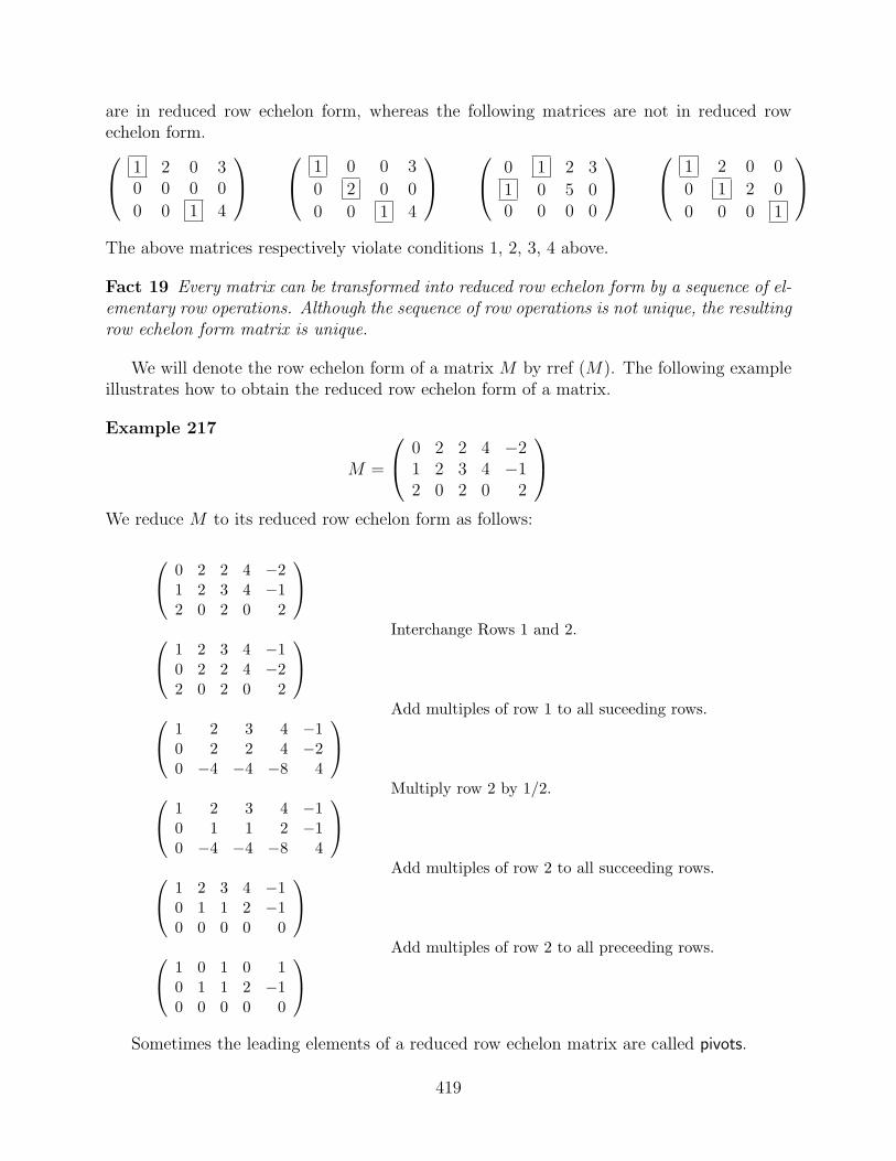
are in reduced row echelon form, whereas the following matrices are not in reduced rowechelon form.

1 2 0 30 0 0 0

0 0 1 4

1 0 0 3

0 2 0 0

0 0 1 4

0 1 2 3

1 0 5 00 0 0 0

1 2 0 0

0 1 2 0

0 0 0 1

The above matrices respectively violate conditions 1, 2, 3, 4 above.

Fact 19 Every matrix can be transformed into reduced row echelon form by a sequence of el-ementary row operations. Although the sequence of row operations is not unique, the resultingrow echelon form matrix is unique.

We will denote the row echelon form of a matrix M by rref (M). The following exampleillustrates how to obtain the reduced row echelon form of a matrix.

Example 217

M =

0 2 2 4 −21 2 3 4 −12 0 2 0 2

We reduce M to its reduced row echelon form as follows:

0 2 2 4 −21 2 3 4 −12 0 2 0 2

Interchange Rows 1 and 2.

1 2 3 4 −10 2 2 4 −22 0 2 0 2

Add multiples of row 1 to all suceeding rows.

1 2 3 4 −10 2 2 4 −20 −4 −4 −8 4

Multiply row 2 by 1/2.

1 2 3 4 −10 1 1 2 −10 −4 −4 −8 4

Add multiples of row 2 to all succeeding rows.

1 2 3 4 −10 1 1 2 −10 0 0 0 0

Add multiples of row 2 to all preceeding rows.

1 0 1 0 10 1 1 2 −10 0 0 0 0

Sometimes the leading elements of a reduced row echelon matrix are called pivots.

419

Gauss-Jordan procedure for solving systems of linear equations. Recall the prob-lem of solving the system of scalar linear equations (27.1) or their vector/matrix counterpart(27.2). The Gauss-Jordan procedure is a systematic method for solving such equations. Onesimply uses elementary row operations to transform the augmented matrix [Ab] into its re-duced row echelon form which we denote by [A b]. Since [A b] is obtained from [A b] byelementary row operations, the set of vectors x which satisfy Ax = b is exactly the same asthe set which satisfy Ax = b. However, since [A b] is in reduced row echelon form, it canbe simply determined whether or not the equation Ax = b has a solution for x, and, if asolution exists, to determine all solutions.

Example 218 Determine whether or not the following system of linear equations has asolution. If a solution exists, determine whether or not it is unique; if not unique, obtain anexpression for all solutions and give two solutions.

y − 2z = 4x− y = 1

3x− 3y + 4z = −9−2y + 10z = −26

Here the augmented matrix is given by

(A b

)=

0 1 −2 41 −1 0 13 −3 4 −90 −2 10 −26

Carrying our elementary row operations, we obtain

0 1 −2 41 −1 0 13 −3 4 −90 −2 10 −26

−→

1 −1 0 10 1 −2 43 −3 4 −90 −2 10 −26

−→

1 −1 0 10 1 −2 40 0 4 −120 −2 10 −26

−→

1 −1 0 10 1 −2 40 0 4 −120 0 6 −18

−→

1 −1 0 10 1 −2 40 0 1 −30 0 6 −18

−→

1 −1 0 10 1 −2 40 0 1 −30 0 0 0

−→

1 −1 0 10 1 0 −20 0 1 −30 0 0 0

−→

1 0 0 −10 1 0 −20 0 1 −30 0 0 0

The reduced row echelon form of [A b] (the last matrix above) tells us that the originalequations are equivalent to:

x = −1

y = −2

z = −3

Thus, the original equations have a unique solution given by x = −1, y = −2 and z = −3.

420

From the above procedure we see that there are three possibilities when it comes tosolving linear equations:

1) A unique solution.

2) Infinite number of solutions.

3) No solution.

421

MATLAB.

help rref

RREF Reduced row echelon form.

R = RREF(A) produces the reduced row echelon form of A.

[R,jb] = RREF(A) also returns a vector, jb, so that:

r = length(jb) is this algorithm’s idea of the rank of A,

x(jb) are the bound variables in a linear system, Ax = b,

A(:,jb) is a basis for the range of A,

R(1:r,jb) is the r-by-r identity matrix.

[R,jb] = RREF(A,TOL) uses the given tolerance in the rank tests.

Roundoff errors may cause this algorithm to compute a different

value for the rank than RANK, ORTH and NULL.

See also RREFMOVIE, RANK, ORTH, NULL, QR, SVD.

Overloaded methods

help sym/rref.m

Exercises

Exercise 157 Determine whether or not the following system of linear equations has asolution. If a solution exists, determine whether or not it is unique, and if not unique,obtain an expression for all solutions.

x1 − x2 + 2x3 + x4 = 5x1 − x2 + x3 = 3

−2x1 + 2x2 + 2x4 = −22x1 − 2x2 − x3 − 3x4 = 0

Exercise 158 Determine whether or not the following system of linear equations has asolution. If a solution exists, determine whether or not it is unique; if not unique, obtain anexpression for all solutions and given two solutions.

x1 − 2x2 − 4x3 = −12x1 − 3x2 − 5x3 = −1x1 + 2x3 = 1x1 + x2 + 5x3 = 2

Exercise 159 Determine whether or not the following system of linear equations has asolution. If a solution exists, determine whether or not it is unique; if not unique, obtain an

422

expression for all solutions and give two solutions.

x1 − 2x2 x3 − 2x4 = −1−3x1 + 7x2 − 3x3 + 7x4 = 4

2x1 − x2 + 2x3 − x4 = 2

Exercise 160 Determine whether or not the following system of linear equations has asolution. If a solution exists, determine whether or not it is unique; if not unique, obtain anexpression for all solutions and give two solutions.

x2 + x4 = 22x1 + 3x2 + 2x3 + 3x4 = 8x1 + x2 + x3 + x4 = 3


x1 − 2x2 − 4x3 = −12x1 − 3x2 − 5x3 = −1x1 + 2x3 = 1x1 + x2 + 5x3 = 2


y − 2z = 4x− y = 1

3x− 3y + 4z = −9−2y + 10z = −26

Exercise 163 We consider here systems of linear equations of the form

Ax = b

with x =

x1

x2

x3

.

For each of the following cases, we present the reduced row echelon form of the augmentedmatrix [A b ]. Determine whether or not the corresponding system of linear equations has asolution. If a solution exists, determine whether or not it is unique; if not unique, obtain anexpression for all solutions and given two solutions.

(a)

1 5 0 00 0 1 00 0 0 1

(b)

1 −2 0 60 0 1 40 0 0 0

(c)

1 2 0 00 0 1 00 0 0 10 0 0 0

(d)

1 0 0 00 1 0 00 0 1 00 0 0 1

423

27.2 Subspaces

Recall that a vector space is a set equipped with two operations, vector addition and mul-tiplication by a scalar, and these operations must satisfy certain properties. The followingconcept generalizes the notion of a line or a plane which passes through the origin.

A non-empty subset S of a vector space is a subspace if for every pair of elements x, y inS and every pair of scalars α, β, the vector αx + βy is contained in S.

In other words, a subset of a vector space is a subspace if it is closed under the operationsof addition and multiplication by a scalar. Note that a subspace can be considered a vectorspace (Why?). An immediate consequence of the above definition is that a subspace mustcontain the zero vector; to see this consider α and β to be zero.

Example 219 Consider the set of real 2-vectors x which satisfy

x1 − x2 = 0

This set is a subspace of IR2. Note that the set of vectors satisfying

Figure 27.1: A simple subspace

x1 − x2 − 1 = 0

is not a subspace.

Example 220 Consider any real m × n matrix A and consider the set of real n-vectors xwhich satisfy

Ax = 0

This set is a subspace of IRn.

Example 221 The set of real matrices of the form(

α ββ γ

)

is a subspace of the space of real 2× 2 matrices.

Example 222 As a more abstract example of a subspace space, let V be the set of con-tinuous real-valued functions which are defined on the interval [0,∞)and let addition andscalar multiplication be as defined earlier Suppose W be the subset of V which consists ofthe differentiable functions V . Then W is a subspace of V .

424

27.3 Basis

27.3.1 Span (not Spam)

Consider a bunch X of vectors. A linear combination of these vectors is a vector which canbe expressed as

α1x1 + α2x

2 + . . . + αmxm

where each xi is in the bunch and each αi is a scalar.

The span of a bunch X of vectors is the set of all vectors of the form

α1x1 + α2x

2 + . . . + αmxm

where each xi is in the bunch and each αi is a scalar; it is denoted by spanX .

In other words, the span of a bunch of vectors is the set of all linear combinations ofvectors from the bunch.

Exercise 164 Show that spanX is a subspace.

Example 223

span

(10

),

(01

)= IR2

To see this, note that any element x of IR2 can be expressed as(

x1

x2

)= x1

(10

)+ x2

(01

)

Example 224

span

(1 00 0

),

(0 10 0

),

(0 01 0

),

(0 00 1

)= IR2×2

To see this, note that any element A of IR2×2 can be expressed as:(

a11 a12

a21 a22

)= a11

(1 00 0

)+ a12

(0 10 0

)+ a21

(0 01 0

)+ a22

(0 00 1

)

Fact 20 Consider a bunch X of vectors. The following ‘experiences’ do not affect span.

(a) Multiplication of one of the vectors by a nonzero scalar.

(b) Replacing a vector by the sum of itself and a scalar multiple of another (different)vector in the bunch.

(c) Removal of a vector which is a linear combination of other vectors in the bunch.

(d) Inclusion of a vector which is in the span of the original bunch.

425

Span and rref. One can use rref to solve the following problem. Given a bunch of n-vectors x1, x2, · · · , xm and another n-vector b, determine whether or not b is in the span ofthe bunch. To solve this problem, consider any linear combination α1x

1+α2x2+. . .+αmxm of

the vectors x1, x2, · · · , xm. Let A be the matrix whose columns are the vectors x1, x2, · · · , xm,that is,

A =(

x1 x2 · · · xm)

and let α be the m-vector whose components are α1, · · · , αm, that is,

α = [ α1 α2 · · · αm ]T .

Then the above linear combination can be expressed as

α1x1 + α2x

2 + . . . + αmxm =(

x1 x2 · · · xm)

α1

α2...

αm

= Aα .

Thus, b is in the span of the bunch if and only if the equation

Aα = b

has a solution for α. One can determine whether or not a solution exists by consideringM = rref(M) where

M = [A b] =(

x1 x2 · · · xm b)

.

Example 225 Suppose we wish to determine whether or not the vector (1, 1,−1) is a linearcombination of the vectors

211

,

031

,

−1

10

.

Since

rref

2 0 −1 11 3 1 11 1 0 −2

=

1 0 −0.5 00 1 0.5 00 0 0 1

,

it follows that the first vector is not a linear combination of the remaining three.

27.3.2 Linear independence

A bunch of vectors, x1, x2, . . . , xm is linearly dependent if there exist scalars α1, α2, . . . , αm,not all zero, such that

α1x1 + α2x

2 + . . . + αmxm = 0 (27.4)

The bunch is linearly independent if it is not linearly dependent, that is, the bunch is linearlyindependent if and only if (27.4) implies that

α1, α2, . . . , αm = 0

426

If the bunch consists of a single vector, then it is linearly independent if and only if thatvector is not the zero vector. If a bunch consists of more than one vector, then it is linearlydependent if and only if one of the vectors can be expressed as a linear combination of thepreceding vectors in the bunch, that is for some j,

xj = β1x1 + β2x

2 + . . . + βj−1xj−1

for some scalars βi.

Example 226 The following bunches of vectors are linearly dependent.

(i) (00

)

(ii) (11

),

(22

)

(iii)

123

,

765

,

321

Why?

(iv) (1 00 1

),

(2 00 2

)

Example 227 The following bunches of vectors are linearly independent.

(a) (11

)

(b) (10

),

(01

)

(c)

123

,

765

427

(d)

01234

494

,

0056474

,

0000

20311

To see this:

α1

01234

494

+ α2

0056474

+ α3

0000

20311

=

000000

impliesα1 = 02α1 + 5α2 = 04α1 + 4α2 + 203α3 = 0

The first equation implies α1 = 0; combining this with the second equation yieldsα2 = 0; combining these results with the last equation produces α3 = 0. So, nonontrivial linear combination of this bunch equals zero; hence the bunch is linearlyindependent.

(e) (1 00 0

),

(0 10 0

),

(0 01 0

),

(0 00 1

)

Exercise 165 Useful generalization of example 227 (d)Consider a bunch of m vectors in IRn (m ≤ n) which have the following structure.

0...0

x1n1.........

,

0......0

x2n2......

, . . . ,

0.........0

xmnm

...

x1n1

, x2n2

, . . . , xmnm6= 0

In words, the first ni−1 components of the i-th vector are zero; its ni component is nonzero;and n1 < n2 < . . . < nnm .

Prove that this bunch is linearly independent.

428

• Consider a bunchx1, x2, . . . , xm

of vectors. It can readily be shown that:

Fact 21 The following ‘experiences’ do not affect linear independence status.

(a) Multiplication of one of the vectors by a nonzero scalar.

(b) Replacing a vector by the sum of itself and a scalar multiple of another (different)vector in the bunch.

(c) Removal of a vector from the bunch.

(d) Inclusion of a vector which is not in the span of the original bunch.

Using rref to determine linear independence. Suppose we want to determine whetheror not a bunch of n-vectors, x1, x2, · · · , xm, are linearly independent. We can achieve thisusing rref. To see this, consider any linear combination α1x

1+α2x2+. . .+αmxm of the vectors

x1, x2, · · · , xm. Let A be the n × m matrix whose columns are the vectors x1, x2, · · · , xm,that is,

A =(

x1 x2 · · · xm)

,

and let α be the m-vector whose components are α1, · · · , αm, that is,

α = [ α1 α2 · · · αm ]T .

Then the above linear combination of vectors can be expressed as

α1x1 + α2x

2 + . . . + αmxm =(

x1 x2 · · · xm)

α1

α2...

αm

= Aα .

Thus the linear combination is zero if and only if Aα = 0. Letting A be the reduced rowechelon form of A, it follows that α satisfies Aα = 0 if and only if Aα = 0. So, the columnsof A are linearly independent if and only if the columns of A are linearly independent. More-over, a column of A is a linear combination of the preceding columns of A if and only if thecorresponding column of A is the same linear combination of the preceding columns of A.From the above observations, we can obtain the following results where A is the reduced rowechelon form of A.

(a) The vectors are linear independent if and only if every column of A contains a leadingelement, that is, the number of leading elements of A is the same as the number of vectors.

(b) If A has a zero column, then the corresponding x-vector is zero; hence the vectors arelinearly dependent.

429

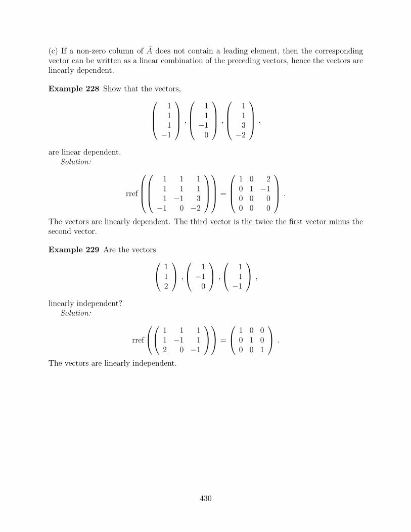
(c) If a non-zero column of A does not contain a leading element, then the correspondingvector can be written as a linear combination of the preceding vectors, hence the vectors arelinearly dependent.

Example 228 Show that the vectors,

111

−1

,

11

−10

,

113

−2

,

are linear dependent.Solution:

rref

1 1 11 1 11 −1 3

−1 0 −2

=

1 0 20 1 −10 0 00 0 0

.

The vectors are linearly dependent. The third vector is the twice the first vector minus thesecond vector.

Example 229 Are the vectors

112

,

1−1

0

,

11

−1

,

linearly independent?Solution:

rref

1 1 11 −1 12 0 −1

=

1 0 00 1 00 0 1

.

The vectors are linearly independent.

430

27.3.3 Basis

A basis for a vector space is a bunch of linearly independent vectors whose span is the space.

A vector space is called finite dimensional if it has a finite basis; otherwise it is infinitedimensional.

For a finite dimensional vector space V , it can be shown that the number of vectors inevery basis is the same; this number is called the dimension of the space and is denoteddim V . We refer to a vector space with dimension n as an n-dimensional space. In ann-dimensional space, every bunch of more than n vectors space must be linearly dependent,and every bunch of n linearly independent vectors must be a basis.

Example 230 The following vectors constitute a basis for IR2 (Why?) :

(10

),

(01

)

Hence IR2 is a 2-dimensional space (Big surprise!).

Example 231 The following vectors constitute a basis for IR2×2 (Why?) :

(1 00 0

),

(0 10 0

),

(0 01 0

),

(0 00 1

)

Hence IR2×2 is a 4-dimensional space.

Example 232 The following vectors constitute a basis for the subspace of example 221.(

1 00 0

),

(0 11 0

),

(0 00 1

)

Exercise 166 Give an example of a basis for IR3 and for IR2×3. What are the dimensionsof these spaces?

Coordinates. If e1, e2, . . . , en is a basis for an n-dimensional vector space, then everyvector x in the space has a unique representation of the form:

x = ξ1e1 + ξ2e

2 + . . . + ξnen

The scalars ξ1, ξ2, · · · , ξn are called the coordinates of x wrt the basis e1, e2, . . . , en. Thusthere is a one-to-one correspondence between any real n-dimensional vector space and IRn.

x→←

ξ1

ξ2...ξn

431

Any linear map from a real n-dimensional V space to a real m-dimensional space W canbe ‘uniquely’ represented by a real m×n matrix; that is, there is a one-to-one correspondencebetween the set of linear maps from V to W and IRm×n. This is achieved by choosing basesfor V and W .

27.4 Range and null space of a matrix

27.4.1 Null space

Consider any real m× n matrix A.

The null space of A, denoted by N (A), is the set of real n-vectors x which satisfy

Ax = 0

that is,

N (A) := x ∈ IRn : Ax = 0

• N (A) is a subspace of IRn. (Exercise)

• The nullity of A is the dimension of its null space, that is,

nullity A := dim N (A)

Determining the null space of a matrix A simply amounts to solving the homogeneousequation Ax = 0. This we can do by obtaining rref (A).

Example 233 A null space calculationLet’s compute a basis for the null space of the following matrix.

A =

0 2 2 4 −21 2 3 4 −12 0 2 0 2

We saw in Example 217 that the reduced row echelon form of A is given by

A =

1 0 1 0 10 1 1 2 −10 0 0 0 0

432

Hence, the vectors in the null space of A are those vectors x which satisfy Ax = 0, that is,

x1 + x3 + x5 = 0x2 + x3 + 2x4 − x5 = 0

these equations are equivalent to

x1 = −x3 − x5

x2 = −x3 − 2x4 + x5

Hence, we can consider x3, x4, x5 arbitrary and for any given x3, x4, x5, the remaining com-ponents x1 and x2 are uniquely determined; hence, all vectors in the null space must be ofthe form

−x3 − x5

−x3 − 2x4 + x5

x3

x4

x5

= x3

−1−1

100

+ x4

0−2

010

+ x5

−11001

where x3, x4, x5 are arbitrary. Thus the null space of A is the subspace spanned by the threevectors:

−1−1

100

0−2

010

−11001

Since the three vectors are linearly independent, they form a basis for the null space of A;hence the nullity of A is 3.

Example 234 Consider any non-zero (angular velocity) matrix of the form:

A =

0 −ω3 ω2

ω3 0 −ω1

−ω2 ω1 0

The null space of A is the set of vectors x which satisfy:

−ω3x2 + ω2x3 = 0ω3x1 − ω1x3 = 0

−ω2x1 + ω1x2 = 0

Every solution to these equations is a scalar multiple of

x =

ω1

ω2

ω3

Hence, the null space of A is the 1-dimensional subspace of IR3 spanned by this vector.

• The set of equilibrium states of a continuous LTI system x = Ax is the null space of A.

• The set of equilibrium states of a discrete LTI system x(k+1) = Ax(k) is the null space ofA− I.

433

27.4.2 Range

Consider a real m× n matrix A.

The range of A, denoted by R(A), is the set of m-vectors of the form Ax where x is ann-vector, that is,

R(A) := Ax : x ∈ IRn

Thus, the range of A is the set of vectors b for which the equation Ax = b has a least onesolution for x.

• R(A) is a subspace of IRm. (Exercise)

The rank of A is the dimension of its range space, that is,

rankA := dim R(A)

Since

A =(

a1 a2 . . . an

)

where a1, a2, . . . , an are the columns of A, it should be clear that

Ax =(

a1 a2 . . . an

)

x1

x2...

xn

= x1 a1 + x2 a2 + . . . + xn an

Hence, the range of a matrix is the set of all linear combinations of its columns. Thus therank of A equals the maximum number of linearly independent columns of A.

From Fact 20 it should be clear that if a matrix A is obtained from a matrix A by asequence of the following operations then A and A have the same range.

(a) Interchanging two columns.

(b) Mutiplication of one of the columns by a nonzero scalar.

(c) Replacing a column by the sum of itself and a scalar multiple of another (different)column in the bunch.

(d) Removal of a column which is a linear combination of other columns in the bunch.

(e) Inclusion of a column which is a linear combination of other columns in the bunch.

Calculation of range basis and rank with rref

Here, we present two ways to calculate a basis for the range of a matrix using rref.

434

Method one: rref(A) A basis for the range of A is given by the columns of A corre-sponding to the columns of rref(A) which contain leading elements. Thus the rank of A isthe number of leading elements in rref(A). This method yields a basis whose members arecolumns from A.

Method two: rref(AT ) Let B be the reduced row echelon form of AT , that is

B = rref(AT ) .

Then the nonzero columns of BT form a basis for the range of A. Thus the rank of A is thenumber of leading elements in rref(AT ).

From the above considerations, it follows that, for any matrix A,

rankAT = rankA

hence,

rankA = maximum number of linearly independent columns of A

= maximum number of linearly independent rows of A

Example 235 (A range calculation) Let’s compute a basis for the range of the matrix,

A =

0 1 1 21 2 3 42 0 2 0

Using Method one, we compute

rref(A) =

1 0 1 00 1 1 20 0 0 0

Since the leading elements of rref(A) occur in columns 1 and 2, a basis for the range of A isgiven by columns 1 and 2 of A, that is

012

,

120

.

Also, the rank of A is two.Using Method two, we compute

rref(AT ) =

1 0 −40 1 20 0 00 0 0

435

Hence,

rref(AT )T =

1 0 0 00 1 0 0

−4 2 0 0

Since columns 1 and 2 are the non-zero columns of rref(AT )T , a basis for the range of A isgiven by columns 1 and 2 of rref(AT )T , that is

10

−4

,

012

.

Again we obtain that the rank of A is two.

Fact 22 If A is an m× n matrix,

dim R(A) + dim N (A) = n

Fact 23 If A and B are two matrices which have the same numbers of columns, then

N (A) = N (B) if and only if R(AT ) = R(BT )

Exercise 167 Picturize the range and the null space of the following matrices.

(2 12 1

) (1 −11 −1

)

Exercise 168

(a) Find a basis for the null space of the matrix,

A =

1 2 3 42 3 4 53 4 5 6

.

(b) What is the nullity of A?

Check your answer using MATLAB.

Exercise 169

(a) Find a basis for the range of the matrix,

A =

1 2 3 42 3 4 53 4 5 6

.

(b) What is the rank of A?

436

Check your answer using MATLAB.

Exercise 170 Obtain a basis for the range of each of the following matrices. Also, what isthe rank and nullity of each matrix?

4 1 −13 2 −31 3 0

0 1 00 0 00 0 1

1 2 3 4 52 3 4 1 23 4 5 0 0

Check your answers using MATLAB.

Exercise 171 Obtain a basis for the the null space of each of the matrices in exercise 170.Check your answers using MATLAB

27.4.3 Solving linear equations revisited

Recall the problem of solving the following m scalar equations for n scalar unknowns x1, x2, . . . , xn:

a11x1 + a12x2 + . . . + a1nxn = b1

a21x1 + a22x2 + . . . + a2nxn = b2...

am1x1 + am2x2 + . . . + amnxn = bm

These equations can be written in matrix form as:

Ax = b

where x is n× 1, b is m× 1 and A is m× n.

• This matrix equation has at least one solution for x if and only if b is in the range of A.This is equivalent to

rank (A b) = rank A

The matrix equation has at least one solution for every b if and only if the range of A isRm, that is, the rank of A is m, or equivalently, the nullity of A is n−m; hence n ≥ m.

• If x∗ is any particular solution of Ax = b, then all other solutions have the form

x∗ + e

where e is in the null space of A.To see this:

Hence, a solution is unique if and only if the nullity of A is zero or equivalently, the rankof A is n; hence n ≤ m.

• It follows from the above that A is invertible if and only if its rank is m and its nullity is0; since rank A + nullityA = n, we must have m = n, that is A must be square.

437

MATLAB A solution (if one exists) to the equation Ax = b can be solved by

x= A\b

>> help orth

ORTH Orthogonalization.

Q = orth(A) is an orthonormal basis for the range of A.

Q’*Q = I, the columns of Q span the same space as the columns

of A and the number of columns of Q is the rank of A.

See also SVD, ORTH, RANK.

>> help rank

RANK Number of linearly independent rows or columns.

K = RANK(X) is the number of singular values of X

that are larger than MAX(SIZE(X)) * NORM(X) * EPS.

K = RANK(X,tol) is the number of singular values of X that

are larger than tol.

>> help null

NULL Null space.

Z = null(A) is an orthonormal basis for the null space of A.

Z’*Z = I, A*Z has negligible elements, and the number of columns

of Z is the nullity of A.

See also SVD, ORTH, RANK.

Exercise 172 Using MATLAB, compute the rank of the matrix(

1 00 δ

)

forδ = 1, 10−3, 10−10, 10−15, 10−16

Any comments?

Range and null space of linear maps

Suppose A is a linear map from an n-dimensional space V to an m-dimensional space W .Then the above definitions and results for matrices can be generalized as follows.

Range of AR(A) := Ax : x ∈ V

438

• R(A) is a subspace of W .

rank A := dim R(A)

Null space of A

N (A) := x ∈ V : Ax = 0• N (A) is a subspace of V .

nullity of A := dim N (A)

Fact 24dim R(A) + dim N (A) = n

• Suppose W = V . Then A is invertible if and only if rankA = n.

Suppose b is given vector in W and consider the equation.

Ax = b

This equation has a solution for x if and only if b is in the range of A. If x∗ is anyparticular solution of Ax = b, then all other solutions have the form

x∗ + e

where e is in the null space of A.........

439

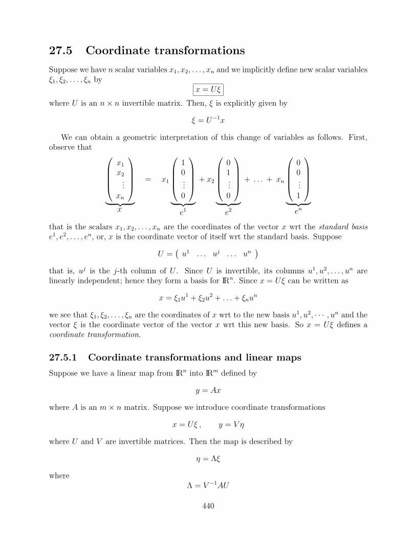
27.5 Coordinate transformations

Suppose we have n scalar variables x1, x2, . . . , xn and we implicitly define new scalar variablesξ1, ξ2, . . . , ξn by

x = Uξ

where U is an n× n invertible matrix. Then, ξ is explicitly given by

ξ = U−1x

We can obtain a geometric interpretation of this change of variables as follows. First,observe that

x1

x2...

xn

︸︷︷︸x

= x1

10...0

︸︷︷︸e1

+ x2

01...0

︸︷︷︸e2

+ . . . + xn

00...1

︸︷︷︸en

that is the scalars x1, x2, . . . , xn are the coordinates of the vector x wrt the standard basise1, e2, . . . , en, or, x is the coordinate vector of itself wrt the standard basis. Suppose

U =(

u1 . . . uj . . . un)

that is, uj is the j-th column of U . Since U is invertible, its columns u1, u2, . . . , un arelinearly independent; hence they form a basis for IRn. Since x = Uξ can be written as

x = ξ1u1 + ξ2u

2 + . . . + ξnun

we see that ξ1, ξ2, . . . , ξn are the coordinates of x wrt to the new basis u1, u2, · · · , un and thevector ξ is the coordinate vector of the vector x wrt this new basis. So x = Uξ defines acoordinate transformation.

27.5.1 Coordinate transformations and linear maps

Suppose we have a linear map from IRn into IRm defined by

y = Ax

where A is an m× n matrix. Suppose we introduce coordinate transformations

x = Uξ , y = V η

where U and V are invertible matrices. Then the map is described by

η = Λξ

whereΛ = V −1AU

440

Recalling that the columns u1, u2, . . . , un of U form a basis for IRn, and the columns v1, v2, . . . , vm

of V form a basis for IRm, we have now the following very useful result.

• Useful result: Suppose

Auj = α1jv1 + α2jv

2 + . . . + αmjvm

Then the matrix Λ = V −1AU is uniquely given by

Λij = αij

that is Λij is the i-th coordinate of the vector Auj wrt the basis v1, v2, . . . , vm, or, the j-thcolumn of Λ is the coordinate vector of Auj wrt the basis v1, v2, . . . , vm.

Example 236 Suppose A is a 2× 2 matrix and there are two linearly independent vectorsu1 and u2 which satisfy:

Au1 = 2u1 and Au2 = u1 + 2u2

Letting U =(

u1 u2), we can use the above useful result to obtain that

U−1AU =

(2 10 2

)

Example 237 Suppose A is a 3 × 2 matrix while U =(

u1 u2)

and V =(

v1 v2 v3)

are invertible 3× 3 and 2× 2 matrices, respectively, which satisfy

Au1 = v1 + 2v3 Au2 = 2v2 + v3

Then, applying the above useful result, we obtain

V −1AU =

1 00 22 1

Proof of useful result. Premultiply Λ = V −1AU by V to get:

V Λ = AU

On the right we have

AU = A(

u1 . . . uj . . . un)

=(

Au1 . . . Auj . . . Aun)

441

And on the left,

V Λ =(

v1 v2 . . . . . . vm)

Λ11 . . . Λ1j . . . Λ1n

Λ21 . . . Λ2j . . . Λ2n...

......

......

...Λm1 . . . Λmj . . . Λmn

=

(Λ11v

1 + · · ·+ Λm1vm ... . . . . . .

... Λ1jv1 + . . . + Λmjv

m

︸︷︷︸j-th column

... . . . . . .... Λ1nv1 + . . . + Λmnvm

)

Comparing the expressions for the j-th columns of AU and V Λ yields

Λ1jv1 + . . . + Λmjv

m = Auj = α1jv1 + . . . + αmjv

m

Since the v1, . . . , vm is a basis we must have Λij = αij.

27.5.2 The structure of a linear map

Consider again a linear map from IRn into IRm defined by

y = Ax

where A is an m × n matrix. Suppose the rank of A is r. Then the dimension of the nullspace of A is n− r. Choose any basis

v1, . . . , vrfor the range of A and extend it to a basis

v1, v2, . . . , vmfor IRm. Choose any basis

ur+1, . . . , unfor the null space of A and extend it to a basis

u1, u2, . . . , un

for IRn.If we introduce the coordinate transformations

y = V η , x = Uξ

whereV = [v1 . . . vm] , U = [u1 . . . un]

442

the original linear map is described by

η = Λξ

whereΛ = V −1AU .

Recall the useful result on coordinate transformations. Since the vectors uj, j = r + 1, . . . , nare in the null space of A we have

Auj = 0 for j = r + 1, . . . , n

Hence, the last r columns of Λ are zero. For j = 1, . . . , r the vector Auj is in the range of A.Hence it can be expressed as a linear combination of the vectors v1, . . . , vr. Consequently,the last m− r rows of Λ are zero and Λ has the following structure:

Λ =

(Λ11 00 0

)

where Λ11 ∈ IRr×r. Since the rank of A equals rank Λ which equals rank Λ11, the matrix Λ11

must be invertible.If we decompose ξ and η as

ξ =

(ξ1

ξ2

), η =

(η1

η2

)

where ξ1 ∈ IRr, ξ2 ∈ IRn−r, η1 ∈ IRr, η2 ∈ IRm−r, then the linear map is described by

η1 = Λ11ξ1

η2 = 0

where Λ11 is invertible.Also, we have shown that any matrix any m× n matrix A can be decomposed as

A = V

(Λ11 00 0

)U−1

where U , V , and Λ are square invertible matrices of dimensions n × n, m ×m, and r × r,respectively, and r is the rank of A.

443

Chapter 28

Appendix D: Inner products

28.1 The usual scalar product on IRn and Cn

Consider any pair x, y of real n-vectors. The scalar product (inner product) of x and y isthe real number given by

〈y, x〉 = y1x1 + . . . + ynxn .

Regarding x and y as real column matrices, we have

〈y, x〉 = yT x .

Suppose x and y are complex n-vectors. If we use the above definition as the definitionof inner product, we won’t have the property that 〈x, x〉 ≥ 0. To see this, note that x = results in x2 = −1. So we define the scalar product (inner product) of x and y to be thecomplex number given by

〈y, x〉 := y1x1 + . . . + ynxn

When x and y are real this definition yields the usual scalar product on IRn. Regarding xand y as column matrices, we have

〈y, x〉 = y∗x

where y∗ is the complex conjugate transpose of y.

We can obtain the usual Euclidean norm from the usual scalar product by noting that

〈x, x〉 = x1x1 + . . . + xnxn

= |x1|2 + |x2|2 + . . . + |xn|2= ‖x‖2 .

Hence

‖x‖ = 〈x, x〉 12 .

445

Properties of 〈·, ·〉. The usual scalar product on IRn or Cn has the following properties.

(i) For every pair of vectors x and y,

〈x, y〉 = 〈y, x〉

(ii) For every vector y, every pair of vectors x1, x2, and every pair of scalars α1, α2,

〈y, α1x1 + α2x

2〉 = α1〈y, x1〉+ α2〈y, x2〉

(iii) For every vector x,

〈x, x〉 ≥ 0

and

〈x, x〉 = 0 if and only if x = 0

For real vectors, property (i) reduces to 〈x, y〉 = 〈y, x〉. By utilizing properties (i) and(ii), we obtain that for every vector x, every pair of vectors y1, y2, and every pair of scalarsα1, α2,

〈α1y1 + α2y

2, x〉 = α1〈y1, x〉+ α2〈y2, x〉

Any scalar valued function on a real (or complex) vector space which has the above threeproperties is defined to be an inner product. A vector space equipped with an inner productis called an inner product space. For example, suppose V is the vector space of all real valuedcontinuous functions defined on the interval [0, 1]. For any two functions f and g in V , let

〈f, g〉 =

∫ 1

0

f(t)g(t) dt .

One may readily show that properties (i)-(iii) above hold.

28.2 Orthogonality

Suppose V is a real (or complex) vector space which is equipped with an inner product 〈·, ·〉.

A vector y is said to be orthogonal to a vector x if

〈y, x〉 = 0

For example, in IR2 the vector (1, 1) is orthogonal to vector (1,−1).

If y is orthogonal to x, then (using property (ii) above) x is orthogonal to y; so, weusually just say x and y are orthogonal.

446

Figure 28.1: Orthogonality

28.2.1 Orthonormal basis

Suppose V is finite dimensional and

b1, b2, . . . bn

is a basis for V . Then this basis is an orthonormal basis if for every i, j,

〈bi, bi〉 = 1

〈bi, b j〉 = 0 when i 6= j

that is each basis vector has magnitude 1 and is orthogonal to all the other basis vectors.

Unitary coordinate transformations

Suppose b1, b2, . . . , bn is an orthonormal basis for Cn and consider the transformation matrix

T =(

b1 b2 . . . bn)

Then

T ∗T =

b1∗

b2∗...

bn∗

(b1 b2 . . . bn

)

=

b1∗b1 b1∗b2 . . . b1∗bn

b2∗b1 b2∗b2 . . . b2∗bn

......

...bn∗b1 bn∗b2 . . . bn∗bn

=

1 0 . . . 00 1 . . . 0...

......

0 0 . . . 1

,

that is, T ∗T = I.

A square complex matrix T is said to be unitary if

T ∗T = I .

If T is unitary, thenT−1 = T ∗ .

447

Example 238 The following matrix is unitary for any θ.

T =

(cos θ − sin θsin θ cos θ

)

Consider a unitary coordinate transformation

x = Tξ

with T unitary. Then for any two n vectors ξ1 and ξ2,

〈Tξ1, T ξ2〉 = (Tξ1)∗Tξ2

= ξ1∗T ∗Tξ2

= ξ1∗ξ2

= 〈ξ1, ξ2〉

hence, 〈Tξ1, T ξ2〉 = 〈ξ1, ξ2〉; that is, unitary transformations preserve the scalar productand, hence, the Euclidean norm.

448

28.3 Hermitian matrices

In this section, the square (n× n) complex matrix P is hermitian, that is

P ∗ = P

If P is real, then hermitian is equivalent to symmetric, that is, P T = P .

• For any complex n-vector x, the scalar x∗Px is real:

x∗Px = (x∗Px)∗

= x∗P ∗x

= x∗Px

Since x∗Px = x∗Px, the scalar x∗Px is real.

• Every eigenvalue λ of P real. Since λ is an eigenvalue of P , there is a nonzero vector vsuch that

Pv = λv

Hencev∗Pv = λv∗v = λ||v||2

Since v∗Pv is real and ||v||2 is nonzero real, λ must be real.

• Suppose v1 and v2 are eigenvectors corresponding to different eigenvalues of P . Then v1

and v2 are orthogonal:

Pv1 = λ1v1

impliesv2∗Pv1 = λ1v2

∗v1

Similarly,v1∗Pv2 = λ2v1

∗v2

Taking the complex conjugate transpose of both sides of this last expression and usingP ∗ = P and λ2 = λ2 yields

v2∗Pv1 = λ2v2

∗v1

Equating the two expressions for v2∗Pv1 yields

λ1v2∗v1 = λ2v2

∗v1

Since λ1 6= λ2, we must have v2∗v1 = 0, that is, v2 is orthogonal to v1.

Actually, the following more general result is true.

Fact 25 Every hermitian matrix has an orthonormal basis of eigenvectors.

449

It now follows that every hermitian matrix P can be expressed as

P = TΛT ∗

where T is a unitary matrix and Λ is a real diagonal matrix whose diagonal elements arethe eigenvalues of P and the number of times an eigenvalue appears equals its algebraicmultiplicity.

28.4 Positive and negative (semi)definite matrices

28.4.1 Quadratic forms

For any square n× n matrix P we can define an associated quadratic form:

x∗Px =n∑

i=1

n∑j=1

pijx∗i xj .

Quadratic forms arise naturally is mechanics. For example, suppose one considers a rigidbody and chooses an orthogonal coordinate system with origin at the body mass center. Ifω is a real 3-vector consisting of the components of the angular velocity vector of the bodyand I is the 3 × 3 symmetric inertia matrix of the body, then the rotational kinetic energyof the body is given by 1

2ωT Iω.

If P is hermitian (P ∗ = P ) then, as we have already shown, the scalar x∗Px is real forall x ∈ Cn. The following result provides useful upper and lower bounds on x∗Px .

• If P is a hermitian n× n matrix, then for all x ∈ Cn

λmin(P )||x||2 ≤ x∗Px ≤ λmax(P )||x||2

where λmin(P ) and λmax(P ) denote the minimum and maximum eigenvalues of P respectively.

Proof. Letting ξ = T ∗x, we have

x∗Px = x∗TΛT ∗x

= ξ∗Λξ

= λ1ξ∗1ξ1 + . . . + λnξ

∗nξn

= λ1|ξ1|2 + . . . + λn|ξn|2

Since, λi ≤ λmax(P ) for i = 1, . . . , n we have λi|ξi|2 ≤ λmax(P )|ξi|2; hence

x∗Px ≤ λmax(P )(|ξ1|2 + . . . + |ξn|2

)= λmax(P )||ξ||2 ;

hence x∗Px ≤ λmax(P )||ξ||2. Also ||ξ|| = ||x||; hence,

x∗Px ≤ λmax(P )||x||2

In an analogous fashion one can show that

x∗Px ≥ λmin(P )||x||2

450

28.4.2 Definite matrices

DEFN. A hermitian matrix P is positive definite (pd) if

x∗Px > 0 for all nonzero x in Cn

We denote this by P > 0.

The matrix P is negative definite (nd) if −P is positive definite; we denote this by P < 0.

Example 239 For

P =

(1 −1

−1 2

)

we have (note the completion of squares trick)

x∗Px = x∗1x1 − x∗1x2 − x∗2x1 + 2x∗2x2

= (x1 − x2)∗(x1 − x2) + x∗2x2

= |x1 − x2|2 + |x2|2

Clearly, x∗Px ≥ 0 for all x. If x∗Px = 0, then x1 − x2 = 0 and x2 = 0; hence x = 0. So,P > 0.


(a) P is positive definite.

(b) All the eigenvalues of P are positive.

(c) All the leading principal minors of P are positive; that is,

p11 > 0

det

(p11 p12

p21 p22

)> 0

...

det(P ) > 0


P =

(1 −1

−1 2

)

Since p11 = 1 > 0 and det(P ) = 1 > 0, we must have P > 0.

>> eig(P)

ans =

0.3820

2.6180

Note the positive eigenvalues.

451

28.4.3 Semi-definite matrices

DEFN. A hermitian matrix P is positive semi-definite (psd) if

x∗Px ≥ 0 for all x in Cn

We denote this by P ≥ 0

The matrix P is negative semi-definite (nsd) if −P is positive semi-definite; we denote thisby P ≤ 0


(a) P is positive semi-definite.

(b) All the eigenvalues of P are non-negative.

(c) All the principal minors of P are non-negative.

Example 241 This example illustrates that non-negativity of only the leading principalminors of P is not sufficient for P ≥ 0. One needs non-negativity of all the principal minors.

P =

(0 00 −1

)

We have p11 = 0 and det(P ) = 0. However,

x∗Px = −|x2|2hence, P is not psd. Actually, P is nsd.

Fact 28 Consider any m× n complex matrix M and let P = M∗M . Then

(a) P is hermitian and P ≥ 0

(b) P > 0 if and only if rank M = n.

Example 242

P =

(1 11 1

)

Since

P =

(11

) (1 1

)

andrank

(1 1

)= 1

P ≥ 0 but P is not pd.

Exercise 173 (Optional)Suppose P is hermitian and T is invertible. Show that P > 0 if and only if T ∗PT > 0.

Exercise 174 (Optional)Suppose P and Q are two hermitian matrices with P > 0. Show that P + εQ > 0 for

all real ε sufficiently small; that is, there exists ε > 0 such that whenever |ε| < ε, one hasP + εQ > 0.

452

28.5 Singular value decomposition

In this section we introduce a matrix decomposition which is very useful for reliable numericalcomputations in linear algebra. First, some notation.

The diagonal elements of an m× n matrix A are

A11, A22, . . . , App where p = minm,nWe say that A is diagonal if all its nondiagonal elements are zero, that is, Aij = 0 for i 6= j.Examples are:

(1 00 2

),

1 00 20 0

,

1 0 0 00 2 0 00 0 0 0

,

(10

).

Theorem 35 (Singular value decomposition) If A is a complex m × n matrix, thenthere exist unitary matrices U ∈ Cm×m and V ∈ Cn×n such that

A = UΣV ∗

where Σ is a diagonal matrix of the same dimension as A and with real nonnegative diagonalelements:

σ1 ≥ σ2 ≥ . . . ≥ σp ≥ 0 p = minm,nIf A is real, then U and V are real.

So, if A is square (m = n), then

Σ =

σ1 0 · · · 00 σ2 · · · 0...

. . ....

0 0 · · · σn

.

When A is “fat” (m < n), we have

Σ =

σ1 0 · · · 0 0 · · · 00 σ2 · · · 0 0 · · · 0...

. . ....

......

0 0 · · · σm 0 · · · 0

.

Finally, a “tall” matrix (m > n) yields

Σ =

σ1 0 · · · 00 σ2 · · · 0...

. . ....

0 0 · · · σn

0 0 · · · 0...

......

0 0 · · · 0

.

453

The scalar σi is called the i-th singular value of A. Let σr be the smallest nonzero singularvalue of A. Then r is smaller than both m and n. Moreover, Σ can be expressed as

Σ =

(Σ11 00 0

)

where Σ11 is the square diagonal invertible matrix given by

Σ11 =

σ1 0 . . . 00 σ2 0

0 0. . .

...0 0 . . . σr

If

U

(Σ11 00 0

)V ∗

is a singular value decomposition of A, then

A∗A = V

(Σ2

11 00 0

)V ∗

Hence, the nonzero singular values of A are uniquely given by

σi =√

λi

where λ1, . . . , λr are the nonzero eigenvalues of the hermitian positive semidefinite matrixA∗A.


A =

(1.2 −0.64 −0.481.6 0.48 0.36

)

has the following singular value decomposition

A =

(0.6 0.80.8 −0.6

)

︸︷︷︸U

(2 0 00 1 0

)

︸︷︷︸Σ

1 0 00 −0.8 0.60 −0.6 −0.8

∗

︸︷︷︸V ∗

Useful facts

• The maximum (or largest) singular value of a matrix satisfies the properties of a norm.Thus, if we consider the set of m× n matrices A and define

||A|| = σmax(A)

454

where σmax(A) denotes the largest singular of A, then the following properties hold:

(a) ||A|| ≥ 0 and ‖A‖ = 0 if and only if A = 0(b) ||λA‖ = |λ|‖A‖(c) ‖A + B‖ ≤ ‖A‖+ ‖B‖ .

In addition to the above usual norm properties, this norm also satisfies

‖A‖ = supx6=0

‖Ax‖‖x‖

where the above vector norms are the usual euclidean vector norms. Thus,

‖Ax‖ ≤ ‖A‖‖x‖

for all x.

• Using the above norm, we can define the distance between two matrices A and B of thesame dimensions as ‖A−B‖.

• The rank of A equals the number of its nonzero singular values.

• Suppose k is a nonegative integer strictly less than the rank r of A. Then in a certainsense (which can be made precise), a matrix of rank k which is “closest” to A is given by

Ak = UΣkV∗

where Σk is the diagonal matrix with diagonal elements

σ1, σ2, . . . , σk, 0, . . . , 0︸︷︷︸p−k zeros

that is, the first k diagonal elements of Σk are the same as those of Σ and the remainingdiagonal elements are zero. Also, the “distance” between Ak and A is σk+1. So, the smallestnonzero singular value σr of A is a measure of the distance between A and the closest matrixof rank r−1.

• Suppose A has rank r and

U =(

u1 u2 . . . um)

, V =(

v1 v2 . . . vn)

Then the vectorsu1, u2, . . . , ur

form an orthonormal basis for the range of A and the vectors

vr+1, vr+2, . . . , vn

form an orthonormal basis for the null space of A

455

MATLAB

>> help svd

SVD Singular value decomposition.

[U,S,V] = SVD(X) produces a diagonal matrix S, of the same

dimension as X and with nonnegative diagonal elements in

decreasing order, and unitary matrices U and V so that

X = U*S*V’.

By itself, SVD(X) returns a vector containing diag(S).

[U,S,V] = SVD(X,0) produces the "economy size"

decomposition. If X is m-by-n with m > n, then only the

first n columns of U are computed and S is n-by-n.

456

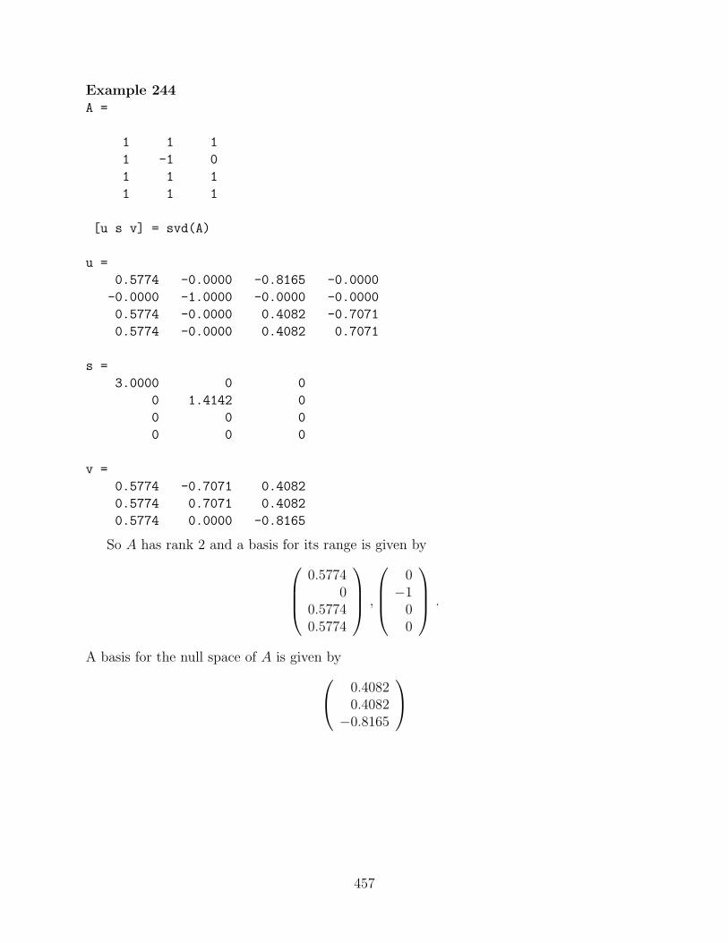
Example 244A =

1 1 1

1 -1 0

1 1 1

1 1 1

[u s v] = svd(A)

u =

0.5774 -0.0000 -0.8165 -0.0000

-0.0000 -1.0000 -0.0000 -0.0000

0.5774 -0.0000 0.4082 -0.7071

0.5774 -0.0000 0.4082 0.7071

s =

3.0000 0 0

0 1.4142 0

0 0 0

0 0 0

v =

0.5774 -0.7071 0.4082

0.5774 0.7071 0.4082

0.5774 0.0000 -0.8165

So A has rank 2 and a basis for its range is given by

0.57740

0.57740.5774

,

0−1

00

.

A basis for the null space of A is given by

0.40820.4082

−0.8165

457

Bibliography

[1] Chen, C.T., Linear System Theory and Design, 3rd Ed., Oxford University Press, 1998.

[2] T. Kailath, T., Linear Systems, Prentice-Hall Information and Systems Science Series,1979.

[3] Khalil, H., Nonlinear Systems, 3rd Ed., Prentice-Hall, 2002.

[4] Vidasagar, M., Nonlinear Systems Analysis, 2nd Ed., Prentice-Hall, 1993.

459

introduction to dynamic systems (network mathematics graduate

Documents