Introduction to Dynamical SystemsBasic Concepts of Dynamics

•  A dynamical system: –  Has a notion of state, which contains all the information upon which the dynamical

system acts. –  A simple set of deterministic rules for moving between states. (Minor exception:

stochastic dynamical systems). –  Iterators. State diagrams that plot xt+1 vs. xt characterize a dynamical system.

•  Example asymptotic behaviors –  Fixed point –  Limit cycles and quasi-periodicity –  Chaotic

•  Limit sets: The set of points in the asymptotic limit. •  Goal: Make quantitative or qualitative predictions of the asymptotic

behavior of a system.

Chaos

•  Chaotic dynamical systems –  Have complicated, often apparently random behavior –  Are deterministic –  Are predictable in the short term –  Are not predictable in the long term –  Are everywhere

•  Turbulence •  Planetary orbits •  Weather •  ?disease dynamics, stock markets and other CAS?

Introduction •  Two main types of dynamical systems:

–  Differential equations –  Iterated maps (difference equations)

•  Primarily concerned with how systems change over time, so focus on ordinary differential equations (one independent variable).

•  Framework for ODE:

•  Phase space is the space with coordinates <x1, … xn> •  We call this a n-dimensional system or an n-th order system.

€

˙ x 1 = f1(x1,x2,...,xn )

˙ x n = fn (x1,x2,...,xn )€

˙ x i ≡ dxi /dt

Linear vs. Nonlinear

•  A system is said to be linear if all xi on the right-hand side appear to the first power only.

•  Typical nonlinear terms are products, powers, and functions of xi, e.g., –  x1x2 –  (x1)3 –  cos x2

•  Why are nonlinear systems difficult to solve? –  Linear systems can be broken into parts and nonlinear systems cannot.

•  In many cases, we can use geometric reasoning to draw trajectories through phase space without actually solving the system.

Example Chaotic Dynamical SystemThe Logistic Map

•  Consider the following iterative equation:

•  We are interested in the following questions: –  What are the possible asymptotic trajectories given different x0 for fixed r?

•  Fixed points •  Limit cycles •  Chaos

–  How do these trajectories change with small perturbations? •  Stable •  Unstable

–  What happens as we vary r?

€

xt+1 = 4rxt (1− xt )

€

xt ,r ∈ [0,1]

The Logistic Map cont.

•  The logistic map:

•  What is the behavior of this equation for different values of r and x0?

–  For xt ==> 0 (stable fixed point)

–  For xt ==> stable fixed point attractor (next slide) note: xt = 0 is a second fixed point (unstable) –  For xt ==> periodic with unstable points and chaos

•  If r < 1/4 then xt+1 < xt

•  However, consider what happens as r increases, between 1/4 and 3/4: –  For an given r, system settles into a limit cycle (period) –  Successive period doublings (called bifurcations) as r increases

€

xt+1 = 4rxt (1− xt )

€

r ≤ 14

€

14

< r <34

€

r >34

Logistic MapState Diagram

€

xt+1 = 4rxt (1− xt )

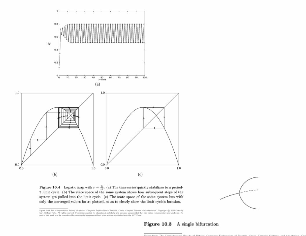
Figure 10.2 goes here.

Transition to Chaos

Characteristics of Chaos

•  Deterministic. •  Unpredictable:

–  Behavior of a trajectory is unpredictable in long run. –  Sensitive dependence on initial conditions.

•  Mixing : The points of an arbitrary small interval eventually become spread over the whole unit interval.

–  Ergodic (every state space trajectory will return to the local region of a previous point in the trajectory, for an arbitrarily small local region).

–  Chaotic orbits densely cover the unit interval. •  Embedded (infinite number of unstable periodic orbits within a chaotic

attractor). –  In a system with sensitivity there is no possibility of detecting a periodic orbit by

running the time series on a computer (limited precision, round-off error). •  Bifurcations.

–  Fractal regions in the bifurcation diagram

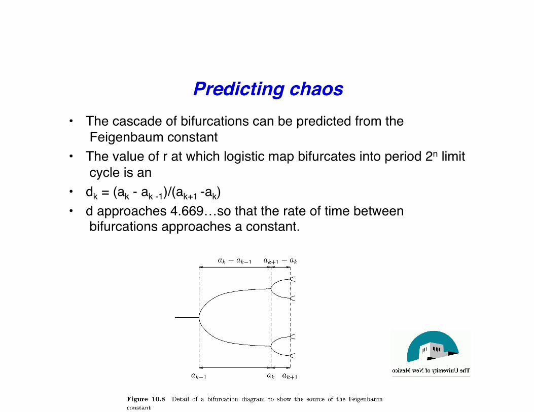
Predicting chaos •  The cascade of bifurcations can be predicted from the

Feigenbaum constant •  The value of r at which logistic map bifurcates into period 2n limit

cycle is an •  dk = (ak - ak -1)/(ak+1 -ak) •  d approaches 4.669…so that the rate of time between

bifurcations approaches a constant.

Information Loss

•  Chaos as Mixing and Folding •  Information loss as loss of correlation from initial conditions

Reading: •  Chapter 11, 12 for Monday •  Complexity in Climate Change Models for Wednesday

Transition to chaos in the Logistic Map http://en.wikipedia.org/wiki/File:LogisticCobwebChaos.gif

The Lorenz Equations http://cs.unm.edu/~bakera/lorenz.html

Chaos and Strange Attractors •  Bifurcations leading to chaos:

–  In the 1 D logistic map, the amount by which r must be increased to get new period doublings gets smaller and smaller for each new bifurcation. –  This continues until the critical point is reached (transition to chaos).

•  Why is chaos important? –  Seemingly random behavior may have a simple, deterministic explanation. –  Contrast with world view based on probability distributions.

•  A formal definition of chaos: –  Chaos is defined by the presence of positive Lyapunov exponents.

•  Working definition (Strogatz, 1994) –  “Chaos is aperiodic long-term behavior in a deterministic system that exhibits

sensitive dependence on initial conditions.” •  Strange Attractors: chaotic systems with an asymptotic dynamic equilibrium.

The system comes close to previous states, but never repeats them. –  Initially, a trajectory through a dynamical system may be erratic. This is known

as the initial transient, or start-up transient. –  The asymptotic behavior of the system is known as equilibrium, steady state,

or dynamic equilibrium. –  The equilibrium states which can be observed experimentally are those

modeled by limit sets which receive most of the trajectories. –  These are called attractors.

Attractor Basins(from Abraham and Shaw, 1984)

•  Basin of attraction: The points of all trajectories that converge to a given attractor.

–  In a typical phase portrait, there will be more than one attractor. •  The dividing boundaries (or regions) between different attractor regions (basins)

are called separatrices. –  Any point not in a basin of attraction belongs to a separatrix.

Example TrajectoriesLinear Vector Fields

Wikipedia, 2007

Shadowing Lemma

Chapter 12: Producer Consumer DynamicsState Spaces: A Geometric Approach

(Abraham and Shaw, 1984) •  An system of interest is observed in

different states. •  These observed states are the target of

modeling activity. •  State space: a geometric model of the set

of all modeled states. •  Trajectory: A curve in the state space,

connecting subsequent observations. •  Time series: A graph of the trajectory.

•  Example: Lotka-Volterra equations: population growth of 2 linked populations

dF/dt = F(a-bS) dS/dt = S(cF-d)

Lotka Volterra

2 spp Lotka Voltera dF/dt = F(a-bS) dS/dt = S(cF-d) a is reproduction rate of Fish b is # of Fish a Shark can eat c is the energy of a Fish (fraction of a new shark) d is death rate of a shark

Compare to single population logistic map

Where is the equilibrium?

€

xt+1 = 4rxt (1− xt )

Tuning parameters to find chaotic regimes

Discrete vs continuous equations continuous chaos requires 3 dimensions (3 populations)

A is a matrix of coefficients that spp j has on spp i A = A11 A12 A13 A21 A22 A23

A31 A32 A33

A = 0.5 0.5 0.1 -0.5 -0.1 0.1

α 0.1 0.1

Lotka Volterra Time Series

Individual Models

•  Implementing chaos as a quasi CA –  Each individual is represented explicitly –  Compare the sizes of the state spaces

•  3 floating point numbers vs •  2 bits per individual x the number of individuals

–  What can we hope to predict in such a complicated system? –  How can we hope to find ecosystem stability? –  Relate to Wolfram’s CA classes

Just one more little complication

•  We’ve gone from simple 1 species population model To a model where multiple populations interact To a model where each individual is represented

•  What if there are differences between individuals? •  Natural selection

–  Geometric increases in population sizes –  Carrying capacity (density dependence) that limits growth –  Heritable variation in individuals that results in differential survival –  Populations become dynamical complex adaptive systems

Reading & References

•  Chaos and Fractals by by H. Peitgen, H. Jurgens, and D. Saupe. Springer-Verlag (1992).

•  Nonlinear Dynamics and Chaos by S. H. Strogatz. Westview (1994). •  J. Gleick Chaos. Viking (1987). •  Robert L. Devaney An Introduction to Chaotic Dynamical Systems.

Addison-Wesley (1989). •  Ralph Abraham and Christopher D. Shaw Dynamics-The Geometry of

Behavior Vol. 1-3 (1984).