introduction to dynamics - uci social sciencesddhoff/omsix.pdf · the conclusion of an observer...

CHAPTER SIX

INTRODUCTION TO DYNAMICS

We begin to develop “participator dynamical systems” on environmentssupported by reflexive frameworks. We introduce the notions of action kerneland participator. For the cases of one and two participator systems, we givea description of the participator dynamics in the language of Markov chains.This chapter is motivational; it deals intuitively with very restricted cases. Inthe next chapter we consider a more general case.

1. Mathematical notation and terminology

The dynamics developed in this chapter makes use of several mathematicalconcepts from the theory of Markov chains. In this section we collect basicterminology and notation for the convenience of the reader.1 We assume afamiliarity with the notions of conditional probability and expectation.

Let (E, E) be a measurable space. The set of measurable functions f :E →R that are bounded is denoted by bE , and the set of measurable nonnegativefunctions by E+.

Recall from chapter two that a kernel P on E is said to be positive if itsrange is in [0, ∞]. It is called a transition probability or a submarkovian kernelif P (e, E) ≤ 1 for all e ∈ E. It is called markovian if P (e, E) = 1 for alle ∈ E. The abbreviation T.P. is sometimes used for transition probability.If P is a positive kernel and f ∈ E+, for example, then P can be viewed asan operator taking f to the function Pf defined by Pf(e) =

∫EP (e, dh)f(h).

1 For more background, beginning readers might refer to Breiman (1969) orNarayan Bhat (1984). For advanced readers we suggest Revuz (1984).

6–1 INTRODUCTION TO DYNAMICS 109

Similarly, if ν is a positive measure on E , then P can be viewed as the operatoron measures νP (A) =

∫Eν(dh)P (h, A) for A ∈ E . The composition or product

of two positive kernels P and Q is the kernel PQ(e, A) =∫EP (e, dh)Q(h, A).

The n-fold product of a kernel P with itself is denoted Pn.

Let (Ω,F , P0) be a probability space and Z = Znn≥0 a sequence ofrandom variables Zn: Ω → E. Such a structure is called a stochastic processwith base space (Ω,F , P0) and state space E. A sequence Gnn≥0 of subσ-algebras of F , such that Gn ⊂ Gn+1 ∀n, is called a filtration on (Ω,F). LetFn = σ(Zm, m ≤ n) and Gn be a filtration such that Gn ⊃ Fn for everyn. The sequence Z = Znn≥0 is called a Markov chain with respect to thefiltration Gnn≥0 if, for every n, the σ-algebras Gn and σ(Zm, m ≥ n) areconditionally independent with respect to Zn; i.e., if for every A ∈ Gn andB ∈ σ(Zm, m ≥ n), P0[A ∩ B|Zn] = P0[A|Zn]P0[B|Zn] a.s. The σ-algebrasFn are referred to as “past” σ-algebras. When we say simply that Z is a Markovchain (with base space (Ω,F , P0)) we mean that it is so with respect to the pastalgebras Fn. Intuitively, a sequence of random variables is a Markov chain ifthe probabilities for passing into the next state are completely determined bythe current state of the system.

A sequence Z = Znn≥0 of random variables is called a homogeneousMarkov chain with respect to the filtration Gn with transition probability P if, forany integersm, n withm < n and any function f ∈ bE , we have E0[f(Zn)| Gm] =Pn−mf(Zm), P0 a.s., where E0 denotes the mathematical expectation op-erator with respect to P0. The probability measure ν defined by ν(A) =P0[Z−1

0 (A)] ≡ P0[Z0 ∈ A], for A ∈ E , is called the starting measure.

Let P be a T.P. on E. It is customary to extend the state space (E, E)to the space (E∆, E∆), where ∆ is a point not in E called the cemetery, E∆ =E ∪ ∆, and E∆ = σ(E , ∆). P extends to a markovian kernel on (E∆, E∆)by setting P (e, ∆) = 1−P (e, E) if e 6= ∆, and P (∆, ∆) = 1. A canonicalprobability space is the space (Ω,F , P0) where Ω =

∏∞n=0E

(n)∆ , and E

(n)∆ is

a copy of E∆; where the σ-algebra F is generated by the semi-algebra ofmeasurable cylinders of Ω (namely sets of the form

∏∞n=0An, where An ∈ E(n)

∆ ,and An differs from E

(n)∆ for only finitely many n); and where P0 is a probability

measure. A point ω = ωn, n ≥ 0 of Ω is called a trajectory or path. Themapping Zn: Ω → E

(n)∆ taking ω = (ω0, ω1, ω2, . . .) ∈ Ω to its nth entry ωn

is called the nth coordinate mapping. If the sequence Z = Zn of coordinatemappings on the canonical probability space forms a homogeneous Markovchain with T.P. P , we call it the canonical Markov chain with T.P. P .

The shift operator θ is the point transformation on Ω defined by θ(ω0, ω1,

110 INTRODUCTION TO DYNAMICS 6–2

. . . , ωn, . . .) = (ω1, ω2, . . . , ωn+1, . . .). We write θn for the n-fold iteration ofθ: θ(ω0, ω1, . . .) = (ωn, ωn+1, . . .). A stopping time T of the canonical Markovchain Z is a random variable defined on (Ω, F) with range in N ∪ ∞ andsuch that for every integer n the event T = n is in Fn. (N is the set ofnatural numbers including 0.) The σ-algebra associated with T is the family FTof events A ∈ F such that for every n, T = n ∩ A ∈ Fn. Notice that thenthe random variable ZT (ω)(ω) is FT -measurable.

Let G be a group that is locally compact with countable basis (LCCB),and let G denote the σ-algebra of its Borel sets. Given probability measuresµ1, µ2 on G, their convolution µ1 ∗ µ2 is defined to be the probability measurewhich assigns to K ∈ G the measure (µ1∗µ2)(K) =

∫ ∫1K(x+y)µ1(dx)µ2(dy).

A right (left) random walk on G is a Markov chain with state space (G, G) andtransition probability εg ∗µ (µ∗εg), where µ is a probability measure on (G, G)which is called the law of the random walk, and εg is Dirac measure supportedat the point g ∈ G. On an abelian group there is only one random walk of lawµ, and it is invariant under translations.

2. Fundamentals of dynamics

The conclusion of an observer O’s perceptual inference is represented, as wehave discussed, by a probability measure η(s, ·). This conclusion is true in agiven semantics, according to Definition 4–3.5, if η(s, ·) is the actual regularconditional distribution, given s, of the measurable functions Xt (defined in4–3.1). Xt is a sequence of random variables indexed by a discrete time t,taking values in configuration space X, and whose domain is some unspecifiedprobability space Ω. In extended semantics (4–4) there is a set B of objectsof perception; for each t, a value of Xt is associated with an interaction of Owith an element of B. These interactions are called channelings. In the caseof an environment supported by a reflexive framework (5–2.6) we have a setof observers B which is also the set of objects of perception for each of itsmembers. At each instant of “reference” time (which, as we shall see, is notthe time t of the random variables Xt) the totality of channeling interactionsat that instant is described by a subset L of B and a relation χ on L as in 5–3.

We now begin to construct a class of models for environments supportedby reflexive frameworks; these models are called “participator dynamical sys-tems.” We do this using entities called “participators”; a participator manifests


as an observer in BE at each instant of reference time. The subset D of B atreference time n always contains the set of participator manifestations at timen. The determination of D and χ can be discussed in terms of participators (wediscuss this in 7–2). In the process of this development, an analytical viewpointemerges in which the participators themselves are the center of attention.

This chapter is informal; for clarity we present many of the ideas in specialcases. In the next chapter we provide a formal development.

The motivation for dynamics

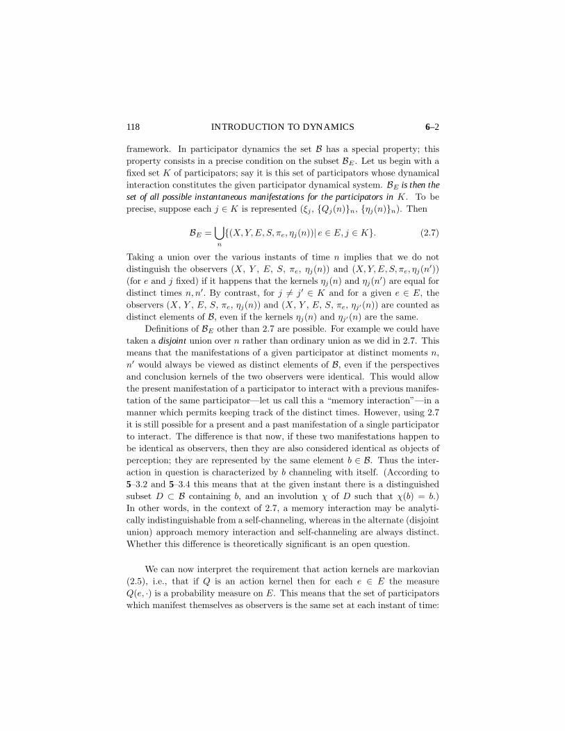
Consider two observers, A and B, in a reflexive framework (X, Y , E, S, π•)of the type shown in Figure 5–2.9. Recall (from 5–2.8) that this means thereexist points a, b ∈ E such that A = (X, Y , E, S, πa, ηA) and B = (X, Y ,E, S, πb, ηB), where ηA, ηB are some conclusion kernels. We depict this inFigure 2.1, where the observers A and B channel to each other. Each makesan inference about the perspective map of the other, i.e., about the point ofE that represents the perspective of the other. Figure 2.1 shows the premises = πa(b) of A’s perceptual inference, and the ray of configuration points x suchthat πa(x) = s (labelled in the figure as π−1

a s). A’s conclusion measure ηA issupported on the set ξ = π−1

a s∩E, which includes b. But ξ includes infinitelymany perspectives other than B’s as well, some of which are indicated by thesmaller dashed circles with numbers above. Thus A is faced with perceptualuncertainty: What was the perspective of the observer that channeled? Wasit 1, 2, b, 3, . . .? In general, A cannot pick just one perspective as the answerto this question. Instead A concludes that it is perspective 1 with probabilityP1, perspective 2 with probability P2, perspective b with probability Pb, andso on. This is the content of A’s conclusion measure ηA(s, ·).

How is A’s conclusion measure ηA(s, ·) to be chosen? On what basiscan A conclude that the other observer’s perspective was 1 with probabilityP1, 2 with probability P2, etc? The answer we give is roughly as follows. Amarkovian dynamics of perspectives naturally arises in the context of reflexiveframeworks. That observers in the framework perceive truly means that theirη’s should be related to the asymptotic behavior of this dynamics. Intuitively,the probability assigned by η(s, ·) to a point e ∈ E should be a conditionalprobability derived from the frequency with which the perspective correspond-ing to that e is adopted by participators in the given dynamical context. Inthis sense, the given dynamics plays the role of the “environment” in whichthese observers are embedded. To make these ideas more precise, we begin by


X

B Aab

πas

1234

-1s

FIGURE 2.1. Perceptual uncertainty in a reflexive framework.

discussing how a dynamics of perspectives arises on reflexive frameworks.When A and B channel, the premise s of A’s perceptual inference greatly

restricts what A can conclude about B’s perspective. Yet A has, in gen-eral, infinitely many choices remaining, for B’s perspective could be any inπ−1a s ∩ E. Suppose A and B retain their perspectives after channeling.

Then if they channel again A has precisely the same set of choices—and thesame ambiguity—regarding B’s perspective as before. In other words, if theobservers do not alter their perspectives after an observation then there is nopoint to further observations. A can channel with B as many times as you like,but the same premise s will result every time, and with it the same ambiguityof interpretation. Moreover, should A and B never change perspectives thewhole question of how ηA is chosen would be trivial: the ideal ηA(s, ·) wouldbe Dirac measure supported on b, and ηA(s′, ·) for s′ 6= s would need not bedefined. Indeed, the construction of reflexive frameworks would be pointless.

Let us, then, allow observers in a reflexive framework to change perspectivefollowing a channeling. That is, let us allow some kind of dynamics of per-spectives on reflexive frameworks. Several questions immediately arise. Howshall observers change perspective? Since the perspective of an observer in areflexive framework (together with its conclusion measure) is its only means ofindividuation, does not a change in perspective actually mean a change in ob-


server? If so, then what is it that is manifesting itself as a different observer ateach step of the dynamics? Furthermore, dynamics requires sequence. Whatis the formal structure of this sequence? What is the formal structure of thedynamics? How, precisely, shall η be related to the resulting dynamics? Weconsider these questions in turn here, and in succeeding chapters.

Action kernels

How should we allow observers to change perspective in reflexive frameworks?There are two basic issues. First, what information should be used to selectthe new perspective of an observer after a channeling? Second, should thenew perspective be chosen deterministically or probabilistically? We discussthese issues in the context of Figure 2.2. This figure shows observers A andB channeling to each other. In consequence of the channeling, A’s premise issA, and B’s premise is sB . The figure shows A changing its perspective fromπa to πa′ , and B changing from πb to πb′ . Of course, after these changes Aand B are no longer the same observers since they no longer have the sameperspectives. We denote the new observers A′ and B′. As can be seen inthe figure, the only information available to choose A’s new perspective isits current perspective and the premise sA. Similarly, mutatis mutandis, forB. Therefore, for maximum generality, we assume that an observer’s nextperspective is some function of its current perspective and current premise.Shall this function be deterministic or probabilistic? Again, for maximumgenerality, we assume that the next perspective is chosen probabilistically,according to some measure. (The deterministic case is the special case that themeasure governing the choice of next perspective is a Dirac measure.) Further,we assume this measure to be a probability measure; after we introduce thenotion of participator, we will interpret this assumption.

In light of these considerations, we could propose that the change in per-spective of an observer A should be governed by a probability measure thatis selected based on A’s current perspective and current premise. However, asense of symmetry suggests that A’s probability measure should depend noton its absolute perspective, but on the “difference” between its perspectiveand that of B. Symmetry also suggests that the probability that A moves toA′ should depend only on the “difference” in perspective between A and A′.Now to talk about differences of perspective in E requires some structure onE. For instance, E might be a principal homogeneous space for some groupof “translations.” More generally, the minimum structure necessary here is a


X

B Aab

sAsB

a’

b’

B’

A’

FIGURE 2.2. Changing perspective on a reflexive framework.

symmetric framework (Definition 5–5.1). However, since the purpose of thischapter is to introduce basic ideas of observer dynamics, we defer (until chap-ter seven) a systematic presentation at this level of generality. Throughoutthis chapter we assume, for simplicity,

Assumption 2.3. We are working in a symmetric framework (X, Y , E, S,G, J , π) in which G = X is an abelian group written additively and J = E

is a subgroup. Equivalently, we can say that (X,Y,E, S, π•) is a reflexiveframework in which X is an abelian group, E ⊂ X is a subgroup, and thereexists a map π:X → Y such that for each e ∈ E, πe(x) = π(x− e).

Thus we can speak of “differences in perspective” without thinking twice.The reader may rely for intuition on examples like Example 5–4.3: one canthink of X as Rn (with vector addition as the group operation) and E as ameasure zero subgroup thereof.

We return now to the question of the probability measure governing changesin perspective. In light of our assumptions, this is a measure on a group E,


telling how probable are various translations from the current perspective. Wecan capture the dependence of the measure on the observer’s current premiseby associating to each premise s of the observer a measure on the group oftranslations that acts on E. The appropriate mathematical device to do thisis a kernel Q that we call an action kernel. For each premise s, the measureQ(s, ·) is a probability measure on the group of translations that acts on E,(the group being, in this chapter, E itself).

X

B Aab

sA

sB

FIGURE 2.4. Action kernels. The shading of the upper circular region representsthe density of the probability distribution QA(sA, ·). Similarly, the shading of thelower circular region represents the density of the probability distribution QB(sB , ·).

These notions are illustrated in Figure 2.4. Once again, two observers Aand B channel with each other. A’s premise is sA. The measure QA(sA, ·),derived from A’s action kernel QA, is depicted by a shaded disk with a dashedline drawn from A to the center of the disk. The darkness of a region within thisdisk encodes the probability that A will adopt a perspective in that region asits next perspective. Darker regions are more probable than lighter ones. A’sexpected new perspective happens, in the case illustrated, to be the perspectiverepresented by the center of the disk. In general there will be some probabilitythat an observer does not change its perspective after a channeling. (Howeverfor pictorial clarity the disk is not drawn large enough to include A’s ownperspective.)


Definition 2.5. Under Assumption 2.3, an action kernel is a markovian kernelQ:E × E → [0, 1] such that Q(e, ·) = Q(e′, ·) if π(e) = π(e′). Given Q, toeach e1 ∈ E we can associate a kernel Qe1 :E × E → [0, 1] by Qe1(e, Γ) =Q(e− e1, Γ).

Suppose Q is an action kernel. Since Q(e, ·) depends only on π(e) we couldequally well define it as a kernel S × E → [0, 1]. In fact we will sometimeswrite Q(s, ·); this will mean Q(e, ·) for any e such that π(e) = s. SimilarlyQe1(e, ·) depends only on πe1(e). The interpretation of the action kernel is asfollows: Q(e, Γ) is the probability that the observer will change perspectiveby an increment in the set Γ, given that it channeled with an observer whoseperspective differed from its perspective by e. If the first observer is at e1,then Qe1(e1 +e, Γ) is an equivalent way to write this. The terminology “actionkernel,” when used for a given kernel Q:E × E → [0, 1], signals our intentionto consider the family of kernels Qee∈E .

Participators

In our discussion of action kernels we have spoken as though an observer in areflexive framework could change its perspective map π. We said, for instance,that an action kernel gives the probabilities with which an observer mightadopt various new perspectives. Now this way of speaking, though convenient,cannot be correct; the definition of observer does not permit a given observerto change its perspective. On the contrary, the definition requires an observerto have a fixed perspective map π:X → Y . Therefore, the formal entity thatchanges perspective according to the dictates of an action kernel is not itselfan observer. Instead this entity manifests itself at each instant as an observerin the context of a reflexive framework. This new formal entity we call a“participator.”

Definition 2.6. A participator on a reflexive framework (X, Y , E, S, π•) (underAssumption 2.3) is a triple, (ξ, Q(n)n, η(n)n), where n varies over thenonnegative integers, ξ is a probability measure on E, each Q(n) is an actionkernel, and each η(n) is a family of interpretation kernels for the reflexiveframework. (That is, η(n) = ηe(n)e∈E , where, for each e ∈ E, (X, Y , E,S, πe, ηe(n)) is an observer.) If all the Q(n) are equal to a fixed action kernelQ, we denote the participator simply by (ξ,Q, η(n)), and call it a kinematicalparticipator with action kernelQ. If, for some n, a participator A = (ξ, Q(n)n,


η(n)n) on a reflexive framework (X, Y , E, S, π•) has perspective πn, thenwe call the observer An = (X, Y , E, S, πn, η(n)) the manifestation of A at timen. We also say that A manifests as An. A preparticipator is a pair (ξ, Q(n)n)with ξ and Q(n) as in a participator.

The formal definition of participator is based upon the following intu-itions. A participator must have a first perspective; this is the purpose of ξ.The probability measure ξ on E, called the initial measure of the participator,governs the choice of the first perspective of the participator. When we say thata participator is initially “at e” or “has perspective e” we mean a participatorfor which ξ is Dirac measure at e; formally, we write ξ = εe. A participatormust also have a means of changing perspective; this is the purpose of the ac-tion kernels Q(n). The changes in perspective are discrete and sequential, withrespect to a notion of time that we discuss shortly. The notation means thatthe nth change of perspective in this sequence is governed by the action ker-nel Q(n). Since the action kernels give probabilities for change of perspectiveconditioned by premises arising from channelings, the perspective changes ofparticipators are probabilistic and are driven by channelings. The terminology“kinematical participator,” for the special case when all the Q(n) are identi-cal, indicates that this case gives rise to systems with a property analogous toconstant velocity. This does not mean that the motion of the participators is“linear” in the usual geometric sense of the word. Rather, it means that theinstantaneous state-change data (in this case, given by the action kernel) istime invariant.

We discuss shortly a dynamics of perspectives that arises from the mutualobservations of an ensemble of participators in a common reflexive framework.This dynamics is a Markov chain whose state space is a product of copies of E,one for each participator in the ensemble. In this chapter we consider a simpli-fied version of the dynamics which is determined entirely by the action kernelsand initial measures of the participators. To specify a (canonical) Markov chainon some space one need only give its initial measure and transition probability.The initial measure of the markovian dynamics of perspectives is simply theproduct of the initial measures of the participators; we study the transitionprobability in chapter seven. In the special case of kinematical participatorsthe resulting Markov chains are homogeneous. In this case we will sometimesuse the word kinematics rather than dynamics.

A participator dynamics on a reflexive framework incorporates a nond-ualistic model of extended semantics. There is some set B of observers inthe framework; B serves as the objects of perception for each observer in the


framework. In participator dynamics the set B has a special property; thisproperty consists in a precise condition on the subset BE . Let us begin with afixed set K of participators; say it is this set of participators whose dynamicalinteraction constitutes the given participator dynamical system. BE is then theset of all possible instantaneous manifestations for the participators in K. To beprecise, suppose each j ∈ K is represented (ξj , Qj(n)n, ηj(n)n). Then

BE =⋃n

(X,Y,E, S, πe, ηj(n))| e ∈ E, j ∈ K. (2.7)

Taking a union over the various instants of time n implies that we do notdistinguish the observers (X, Y , E, S, πe, ηj(n)) and (X,Y,E, S, πe, ηj(n′))(for e and j fixed) if it happens that the kernels ηj(n) and ηj(n′) are equal fordistinct times n, n′. By contrast, for j 6= j′ ∈ K and for a given e ∈ E, theobservers (X, Y , E, S, πe, ηj(n)) and (X, Y , E, S, πe, ηj′(n)) are counted asdistinct elements of B, even if the kernels ηj(n) and ηj′(n) are the same.

Definitions of BE other than 2.7 are possible. For example we could havetaken a disjoint union over n rather than ordinary union as we did in 2.7. Thismeans that the manifestations of a given participator at distinct moments n,n′ would always be viewed as distinct elements of B, even if the perspectivesand conclusion kernels of the two observers were identical. This would allowthe present manifestation of a participator to interact with a previous manifes-tation of the same participator—let us call this a “memory interaction”—in amanner which permits keeping track of the distinct times. However, using 2.7it is still possible for a present and a past manifestation of a single participatorto interact. The difference is that now, if these two manifestations happen tobe identical as observers, then they are also considered identical as objects ofperception; they are represented by the same element b ∈ B. Thus the inter-action in question is characterized by b channeling with itself. (According to5–3.2 and 5–3.4 this means that at the given instant there is a distinguishedsubset D ⊂ B containing b, and an involution χ of D such that χ(b) = b.)In other words, in the context of 2.7, a memory interaction may be analyti-cally indistinguishable from a self-channeling, whereas in the alternate (disjointunion) approach memory interaction and self-channeling are always distinct.Whether this difference is theoretically significant is an open question.

We can now interpret the requirement that action kernels are markovian(2.5), i.e., that if Q is an action kernel then for each e ∈ E the measureQ(e, ·) is a probability measure on E. This means that the set of participatorswhich manifest themselves as observers is the same set at each instant of time:


participators do not appear or disappear while a scenario is running. To seethis, recall that if Q is the action kernel of a participator A, the measure Q(e, ·)assigns probabilities to A’s perspective at time n + 1 (given that, at time n,A channeled with some participator whose perspective is e). And if Q is notmarkovian, i.e., if Q(e, E) < 1, then there is positive probability that A hasno perspective at time n + 1, so that it is not manifested as an observer inthe framework at that time. However, though A must manifest as an observerat each time n, A’s manifestation need not channel at each time n. In otherwords, the subset L of B which is the domain of the channeling relation attime n may be a proper subset of the set of all participator manifestations attime n. We see, then, that the markovian requirement on action kernels is amatter of convention, not a restrictive assumption: since we do not require theparticipators to channel at every instant, and since the dynamics is driven bychanneling, the net effect on the dynamics is the same whether a participatordoes not manifest at time n, or manifests but does not channel at time n.

Reference and proper timesDynamics requires some notion of time or sequence. Our notion of time in thecontext of participator dynamics is guided in part by the ideas of Einstein:

“ The experiences of an individual appear to us arranged in a seriesof events; in this series the single events which we remember ap-pear to be ordered according to the criterion of ‘earlier’ and ‘later,’which cannot be analyzed further. There exists, therefore, for theindividual, an I-time, or subjective time. This in itself is not mea-surable. I can, indeed, associate numbers with the events, in sucha way that a greater number is associated with the later event thanwith an earlier one; but the nature of this association may be quitearbitrary.”2

The only events in a reflexive framework with which to associate numbersare the discrete acts of observation and the consequent changes in perspective.To each participator, then, we assign a number, called the “proper time” ofthat participator, such that the number increases only when the participatormakes an observation. Every channeling that involves that participator in-creases its proper time. Thus discrete acts of observation constitute the unitsof subjective time in this framework. We will give a more formal treatment

2 Einstein (1956), p. 1.


of proper time in chapter seven; the examples we present in this chapter aresimplified (artificially) so that the proper time of each participator coincideswith “reference time” (defined below).

The setting of the dynamics described here is different from the space-time setting assumed in physics. In place of physical space we have the spaceof possible observer perspectives, and in place of physical time we have thesequence of discrete observations of participators.

A particular channeling may not include the perspectives of some partic-ipators in the dynamics. In this case the proper times of the excluded par-ticipators are not increased, but the proper times of the others are increased.Therefore, even if the proper times of all participators begin with the samevalue, say zero, their proper times will eventually differ due to channelingsthat exclude some participators. We cannot then, in general, take the propertime of any particular participator to be the time parameter of the markoviandynamics of the ensemble. For this we need a time parameter that increasesfor every channeling whether or not that channeling includes a particular par-ticipator. This time parameter we call “reference time.” In a given dynamicalsetting in which we have a fixed set K of participators, we may take the ref-erence time to be a copy of the nonnegative integers, called “R,” which is thedomain of the time index “n” of Definition 2.6 for all the participators in K.Thus in speaking of reference time we are making the assumption that theseindices have a common domain.

The reference time in a given dynamical context (corresponding to a setK of participators) is not the same as the active time in the sense of 4–2.1for the observers in the set BE of 2.7. In fact, reference time is associatedto a set of participators, not to a set of observers. And the reference timeneed not include those instants when the participators channel only to non-distinguished objects of perception. It need only include those instants whenparticipator observations occur, and by the term ‘observation’ we always meana channeling which results in a distinguished premise (which causes the outputof a conclusion, etc.). Now a channeling with a non-distinguished object ofperception may result in a distinguished premise (“false targets”), and aninstant of time in which this occurs (for the manifestation of a participator)would have to be included in reference time. But if no distinguished premisesoccurred at the given instant for any of the participators, then that instantwould be excluded from reference time.

Recall, by contrast, that since the active time of an observer indexes theXt’s, it consists by definition precisely of those instants when the observerreceives any channeling, from a distinguished object of perception or not.


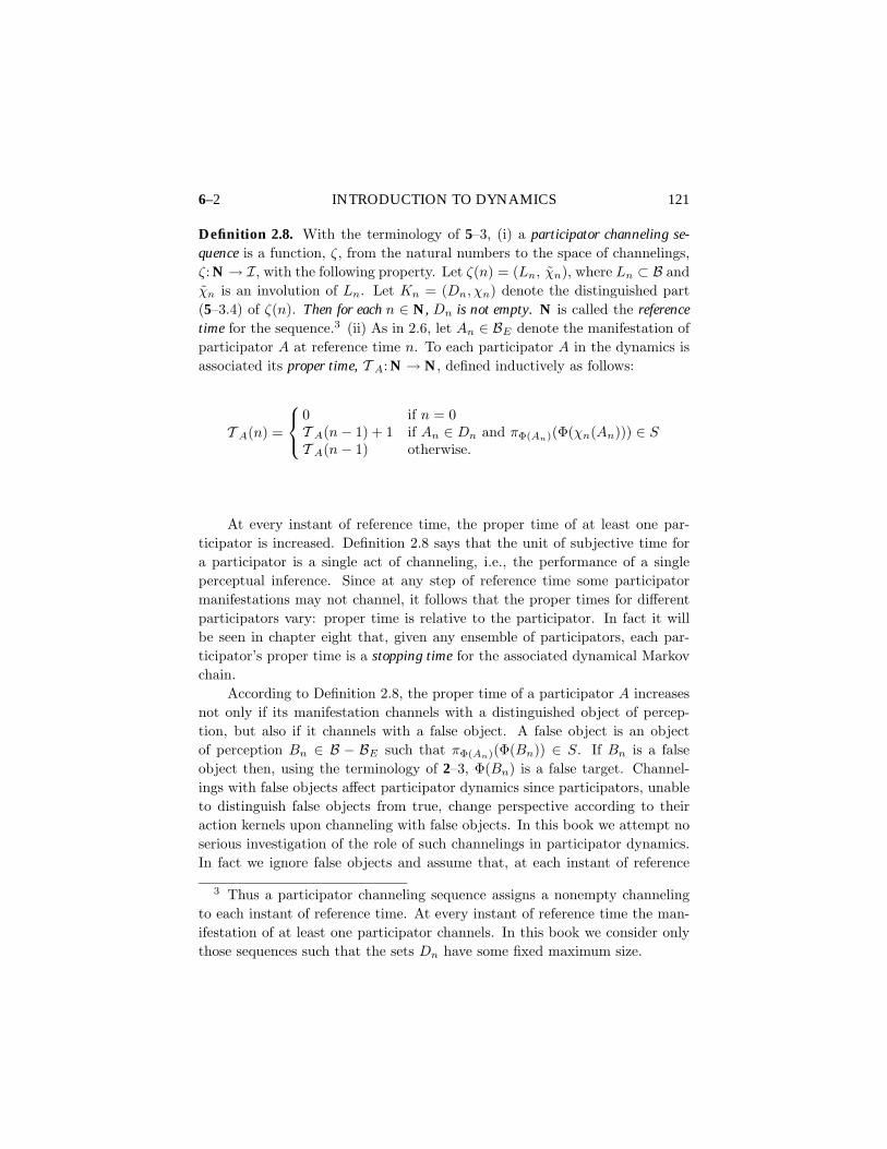
Definition 2.8. With the terminology of 5–3, (i) a participator channeling se-quence is a function, ζ, from the natural numbers to the space of channelings,ζ: N→ I, with the following property. Let ζ(n) = (Ln, χn), where Ln ⊂ B andχn is an involution of Ln. Let Kn = (Dn, χn) denote the distinguished part(5–3.4) of ζ(n). Then for each n ∈ N, Dn is not empty. N is called the referencetime for the sequence.3 (ii) As in 2.6, let An ∈ BE denote the manifestation ofparticipator A at reference time n. To each participator A in the dynamics isassociated its proper time, T A: N→ N, defined inductively as follows:

T A(n) =

0 if n = 0T A(n− 1) + 1 if An ∈ Dn and πΦ(An)(Φ(χn(An))) ∈ ST A(n− 1) otherwise.

At every instant of reference time, the proper time of at least one par-ticipator is increased. Definition 2.8 says that the unit of subjective time fora participator is a single act of channeling, i.e., the performance of a singleperceptual inference. Since at any step of reference time some participatormanifestations may not channel, it follows that the proper times for differentparticipators vary: proper time is relative to the participator. In fact it willbe seen in chapter eight that, given any ensemble of participators, each par-ticipator’s proper time is a stopping time for the associated dynamical Markovchain.

According to Definition 2.8, the proper time of a participator A increasesnot only if its manifestation channels with a distinguished object of percep-tion, but also if it channels with a false object. A false object is an objectof perception Bn ∈ B − BE such that πΦ(An)(Φ(Bn)) ∈ S. If Bn is a falseobject then, using the terminology of 2–3, Φ(Bn) is a false target. Channel-ings with false objects affect participator dynamics since participators, unableto distinguish false objects from true, change perspective according to theiraction kernels upon channeling with false objects. In this book we attempt noserious investigation of the role of such channelings in participator dynamics.In fact we ignore false objects and assume that, at each instant of reference

3 Thus a participator channeling sequence assigns a nonempty channelingto each instant of reference time. At every instant of reference time the man-ifestation of at least one participator channels. In this book we consider onlythose sequences such that the sets Dn have some fixed maximum size.


time, participator manifestations channel only with other participator mani-festations. (As an informal justification for this one might assume that thestatistical properties of the action kernels somehow take into account theseextraneous channelings.) This is the content of the following “closed system”assumption:

Assumption 2.9. Closed system. For each reference time n, Dn is containedin the set of participator manifestations at time n.

One further assumption should be noted. We conceive of the change ofperspectives of participators on a reflexive framework as probabilistic. How-ever, we have not given explicit details of the underlying probability spaceson which the dynamical mechanism depends. Our proposal for the underlyingframework will be made in the next chapter. Here we note only the followingcharacteristic:

Assumption 2.10. Independent action. At any instant of reference time, andgiven the current perspectives of all participators and the current channelinginvolution, the perspectives of the participators at the next instant of referencetime are independent random variables.

For example, suppose we have three participators A, B and C with actionkernels QA, QB and QC respectively, and with channeling involution χ =(A,B) (so that C is not channeled to). Then the probability that, at thenext instant, A ∈ ΓA, B ∈ ΓB , and C ∈ ΓC is

QA,eA(eB ,ΓA)QB,eB (eA,ΓB)1ΓC (eC).

That is, we need simply take a product of the appropriate probabilities for theindividual participators.

3. Kinematics of a single participator

In this section we consider the kinematics of perspectives that arises in a systemconsisting of a single kinematical participator. We find that this kinematics is a


random walk. In the next section we consider a kinematics of two participators.We consider the general case in the next chapter.

Consider a single participator on a symmetric framework (X, Y , E, S, G,J , π) satisfying Assumption 2.3. Let ξ = εe, e ∈ E. The first manifestationof this participator then has perspective map πe, defined by πe(g) = π(g − e),g ∈ X. The only channeling possible, since there is but one participator, isa “self channeling,” viz., a channeling in which χ(e) = e. The participator’spremise is then πe(e), i.e., π(0), where 0 denotes the identity element of ouradditive abelian group E. This applies to each instant of the participator’sproper time and, since there are no other participators, the system is inertat all other instants. It follows from this that the same perceptual premises0 = π(0) ∈ S obtains at each step of the kinematics. And, denoting by Q theaction kernel of the participator, this implies that the same probability measureQ(s0, ·) for the next perspective obtains at each step of the kinematics. Thisimplies that the kinematics is a random walk of law Q(s0, ·) with respect tothe discrete time which is the participator’s proper time and, in this specialcase, the reference time.

4. Kinematics of pairs

We now consider a system involving two kinematical participators. In such asystem each participator might channel with itself, with the other participator,or not at all, at each step of reference time. In this section we assume forsimplicity that each participator channels with the other at each step of thekinematics. In the next chapter we consider the general case.

Again we are in the situation of Assumption 2.3. When two participators,A and B, observe each other, each changes its perspective according to itsaction kernel. This leads to a new difference in their perspectives. This changein the relationship between their perspectives is governed by a kernel P whichwe can define as follows: for each e ∈ E and Γ ∈ E , P (e, Γ) is the probabilitythat, as the result of a change in their perspectives, the new perspective of Brelative to A (i.e., the difference of their new perspectives) will lie in the set Γ,given that the present difference in their perspectives is e. We can compute Pfrom the action kernels of the individual participators as illustrated in Figure4.1. The figure shows two participators with initial perspectives a and b. Theperspective of B relative to A is e (that of A relative to B is −e). After


observing, A changes perspective by an amount dk and B changes perspectiveby an amount dh. This leads to a new difference in perspective e−dk+dh (or−(e− dk + dh)).

Let Q and R denote the action kernels of the participators whose currentperspectives are a and b respectively. Then the probability that A changesperspective by an amount dk given that B’s perspective differs from A’s by anamount e is Q(e, dk). Similarly, the probability that B changes perspective byan amount dh given that A’s perspective differs from B’s by an amount −e isR(−e, dh). The probability of the joint event that A changes by dk and B bydh is, by Assumption 2.10, Q(e, dk)R(−e, dh). That is, the probability thatthe new difference in perspective is e − dk + dh, given that the old differencein perspective was e, is given by Q(e, dk)R(−e, dh). Thus, to determine whatis the probability that the new difference in perspective lies within a regionΓ ∈ E , we simply find the measure of the region (k, h) ∈ E×E| e−k+h ∈ Γwith respect to the product measure Q(e, dk)⊗R(−e, dh) on E × E. This isthe same as the integral∫

E×E1Γ(e− k + h)Q(e, dk)R(−e, dh);

we conclude that P (e, Γ) is this integral.

X

B Aab e

dk

e-dk

+dh

dh

FIGURE 4.1. Two participators change perspective.


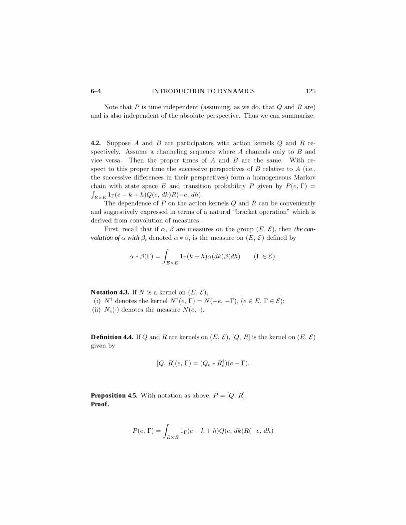
Note that P is time independent (assuming, as we do, that Q and R are)and is also independent of the absolute perspective. Thus we can summarize:

4.2. Suppose A and B are participators with action kernels Q and R re-spectively. Assume a channeling sequence where A channels only to B andvice versa. Then the proper times of A and B are the same. With re-spect to this proper time the successive perspectives of B relative to A (i.e.,the successive differences in their perspectives) form a homogeneous Markovchain with state space E and transition probability P given by P (e, Γ) =∫E×E 1Γ(e− k + h)Q(e, dk)R(−e, dh).

The dependence of P on the action kernels Q and R can be convenientlyand suggestively expressed in terms of a natural “bracket operation” which isderived from convolution of measures.

First, recall that if α, β are measures on the group (E, E), then the con-volution of α with β, denoted α ∗ β, is the measure on (E, E) defined by

α ∗ β(Γ) =∫E×E

1Γ(k + h)α(dk)β(dh) (Γ ∈ E).

Notation 4.3. If N is a kernel on (E, E),(i) N† denotes the kernel N†(e, Γ) = N(−e, −Γ), (e ∈ E, Γ ∈ E);(ii) Ne(·) denotes the measure N(e, ·).

Definition 4.4. If Q and R are kernels on (E, E), [Q, R] is the kernel on (E, E)given by

[Q, R](e, Γ) = (Qe ∗R†e)(e− Γ).

Proposition 4.5. With notation as above, P = [Q, R].Proof.

P (e, Γ) =∫E×E

1Γ(e− k + h)Q(e, dk)R(−e, dh)


=∫E×E

1e−Γ(k − h)Q(e, dk)R(−e, dh);

change variables so that h is replaced by −h:

=∫E×E

1e−Γ(k + h)Q(e, dk)R(−e, −dh)

=∫E×E

1e−Γ(k + h)Q(e, dk)R†(e, dh)

= (Qe ∗R†e)(e− Γ) = [Q, R](e, Γ).

For the moment, let P ′ denote the kernel for the Markov chain of per-spectives of A relative to B. On the one hand, it is geometrically evident thatP ′(e, Γ) = P (−e, −Γ) (where, as above, P denotes the kernel for the perspec-tives of B relative to A). On the other hand, from Proposition 4.5 we find thatP ′ = [Q, R]. We conclude

Proposition 4.6. For any kernels Q, R,

[Q, R] = [R, Q]†.

This may also be verified directly from Notation 4.3 and Definition 4.4.

We close this section with several remarks. First, nothing prevents Aand B from occupying the same perspective in E at a given instant. Second,the situation considered in this section, where each participator channels onlyto the other (and not to itself) is the opposite extreme of that treated inthe previous section, where a participator channels only to itself. To makethe comparison appropriate, imagine two kinematical participators A and B,each channeling only to itself. In this case we would get a Markov chain onE × E; in each factor we would have a random walk, (one for A and onefor B) as in the previous section. These random walks would be completely“uncoupled.” In the situation treated in this section the perspectives of Aand B are completely coupled: it is very unlikely that we would get anythingresembling a random walk by looking at their sequences of states separately(or jointly). In the general setting, the question of the relative frequenciesof cross-channelings and self-channelings in, say, a two participator dynamical


system is described by an additional datum, called a τ -distribution, which wethink of as describing the “informational conductivity” of E. Depending on theτ -distribution, the dynamical chain generated by an ensemble of participatorswith given action kernels will express some degree of coupling of the randomwalks each participator would undergo were there no cross-channelings. Wewill study this in more detail in the next chapter. The main idea here is that,given an ensemble of participators and a τ -distribution, a dynamical Markovchain is generated.

5. True perception among pairs

We have seen that a dynamics of perspectives arises naturally on reflexiveframeworks. Intuitively, the purpose of the dynamics is to allow the participa-tors to “perceive truly,” i.e., to choose conclusion measures η(s, ·) which in factreflect the probabilities of events on the reflexive framework. Specifically, ifparticipator A channels with B, leading to a premise sA, then A should arriveat a conclusion measure ηA(sA, ·) which correctly describes with what proba-bility the perspective of B, relative to A, lies in various subsets of π−1

a (sA)∩E.In this section we specify conditions in which each participator, in a systemof two mutually observing participators, can perceive truly the perspective ofthe other. Chapter eight addresses the issue of true perception formally andin greater generality.

We assume, as in the previous section, that there are no self-channelings;all channelings are cross-channelings. In chapter seven we consider more gen-eral dynamics, but several ideas are revealed by considering the simpler case.

We found in the last section that the kinematics of relative perspectivesfor two participators is markovian with transition probability P . The theoryof Markov chains describes some interesting properties of this kinematics thatare relevant to the problem of true perception. We describe these propertiesinformally now, and formally in the next chapters.

Depending on the details of the transition probability P , one finds that thestate space E of the markovian dynamics contains different “pockets” whichact like traps; if the state of the chain happens to enter one of these pockets,then the chain will forever stay within that pocket almost surely. For thisreason these pockets are called “absorbing sets.” The complement in the statespace of all the absorbing sets is a pool of states called the “transient states.”This is depicted in Figure 5.1, where the white disks represent absorbing sets


E

FIGURE 5.1. Absorbing sets on the state space of a markovian dynamics. Whitedisks represent absorbing sets. Blue regions represent transient states.

and the states outside the disks are the transient states. An absorbing set maycontain infinitely many states. If a chain enters an absorbing set, the chainthen marches probabilistically from state to state within the absorbing set,and almost surely never enters a state outside of the absorbing set.

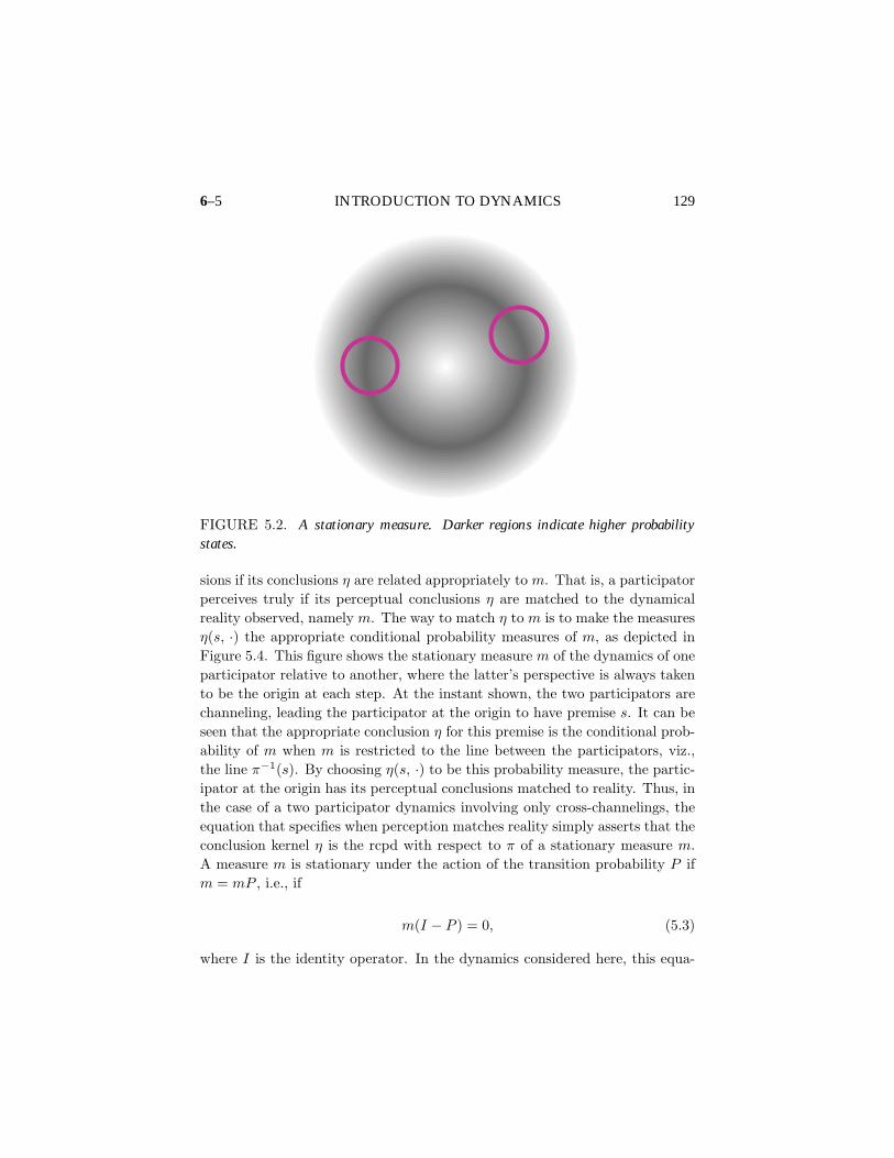
One finds that, for each absorbing set C, there is a unique probabilitymeasure supported on C which describes the long term behavior of the chain,once it is trapped in C. This measure, say m, gives for each subset D of theabsorbing set a probability, m(D); m(D) can be interpreted as the relativefrequency that the trapped chain is found within D over a very long time. Themeasure m is called a “stationary” measure; an example of such a measure fora dynamics of two participators is shown in Figure 5.2. Darker regions indicatehigher frequency states. The little circles drawn over the stationary measureindicate the perspectives each participator happens to adopt at some instantof the dynamics.4

Now if a two participator dynamical chain enters an absorbing set withstationary measure m, then each participator can reach true perceptual conclu-

4 Figure 5.2 does not represent the stationary measure on the original statespace of the Markov chain. The original state space is a product space, E2,where there are two participators in the chain. Figure 5.2 represents the sta-tionary measure on a single copy of E, which describes the perspective of Brelative to A.


FIGURE 5.2. A stationary measure. Darker regions indicate higher probabilitystates.

sions if its conclusions η are related appropriately to m. That is, a participatorperceives truly if its perceptual conclusions η are matched to the dynamicalreality observed, namely m. The way to match η to m is to make the measuresη(s, ·) the appropriate conditional probability measures of m, as depicted inFigure 5.4. This figure shows the stationary measure m of the dynamics of oneparticipator relative to another, where the latter’s perspective is always takento be the origin at each step. At the instant shown, the two participators arechanneling, leading the participator at the origin to have premise s. It can beseen that the appropriate conclusion η for this premise is the conditional prob-ability of m when m is restricted to the line between the participators, viz.,the line π−1(s). By choosing η(s, ·) to be this probability measure, the partic-ipator at the origin has its perceptual conclusions matched to reality. Thus, inthe case of a two participator dynamics involving only cross-channelings, theequation that specifies when perception matches reality simply asserts that theconclusion kernel η is the rcpd with respect to π of a stationary measure m.A measure m is stationary under the action of the transition probability P ifm = mP , i.e., if

m(I − P ) = 0, (5.3)

where I is the identity operator. In the dynamics considered here, this equa-


tion, together with the stipulation that η is the rcpd of m, is the “perception= reality” equation. Note that there are in general many absorbing sets, eachwith its own stationary measure, so that the measure m is not uniquely de-termined even when P is fixed. Therefore, to determine if perception matchesreality, we must be careful to use the appropriate stationary measure.

FIGURE 5.4. A participator’s conclusion measure should be derived as the rcpd ofthe appropriate stationary measure.

Now if the chain never enters an absorbing set, i.e., if the dynamics isnot stable, then there is no stationary probability measure to use to computeη. True perception is not possible. There are no probability measures η(s, ·)that are matched to the dynamical reality. We see that a stable dynamics ofperspectives is necessary for true perception.

In chapter ten we discuss how, to each absorbing set, there are associatedin a natural manner complex-valued eigenfunctions of the transition probabil-ity P . We show that the squared amplitude of these eigenfunctions yields aprobability measure which is stationary or asymptotic (a property, to be dis-cussed later, which is slightly weaker than stationarity).


6. An example

We close this chapter with an illustration of participator dynamics by meansof a specific and elementary example, including a computation of its stationarymeasures. Consider the symmetric framework (X, Y , E, S, G, J , π), where

X = R, E = Z (the integers),

Y = S = 1, 0,−1, G = 〈R,+〉, J = 〈Z,+〉,π(x) = sgn(x) (6.1)

and where the signum function “sgn” is given by

sgn(x) =

1, if x > 0;0, if x = 0;−1, if x < 0.

(6.2)

Suppose we have two participators labelled “1” and “2” respectively, whichchannel with each other at each instant of reference time. As before, we do notallow self-channeling. Both participators are assumed to have the same actionkernel Q, defined as follows:

Q(0, ·) = ε0(·)(where ε0(·) is Dirac measure at 0); if r 6= 0,

Q(r, x) =

ρ, if x = sgn(r);1− ρ, if x = sgn(−r);0, otherwise.

(6.3)

(Here r is the relative position before channeling and x is the participator’schange in position after channeling; we assume that the quantity ρ lies between0 and 1). In words: if a channeling came from the participator’s currentposition, there is no movement. Otherwise, the participator moves one step inthe direction from which the channeling came, with a probability of ρ, or onestep away from that direction, with the complementary probability of 1− ρ.

Imagine that the two participators are initially separated by a nonzero dis-tance. After they channel, their relative distance will either remain unchanged,or will have changed by two units. These are the only possibilities. (If they


were initially at the same position in E, nothing will change.) This is expressedin the following derivation of the dynamical kernel P of the joint markoviandynamics (as introduced in section four above). Note that the dynamics isrelativized; it is a dynamics on the group Z of the relative displacements ofparticipator 2 with respect to participator 1.

1− ρ← • → ρ ρ← • → 1− ρ

∗ ∗ ∗| ∗ ∗ ∗ ∗| ∗ ∗ ∗ ∗© ∗ ∗ ∗ ∗ | ∗ ∗ ∗ ∗| ∗ ∗ ∗ ∗| ∗ ∗ ∗ ∗| ∗ ∗ ∗ ∗© ∗ ∗ ∗ ∗ | ∗ ∗ ∗ ∗| ∗ ∗∗

Participator 2 Participator 1

FIGURE 6.4. A markovian two-participator dynamics with E = Z. The currentrelative separation is r = −5. After a channeling each participator will jump in theindicated directions with the given probabilities.

Proposition 6.5. Let r denote the current relative separation and q therelative separation after channeling. Then the kernel P of the dynamics isgiven byIf r = 0,

P (0, q) = ε0(q). (6.6)

If q = r, r 6= 0,P (r, q) = 2ρ(1− ρ). (6.7)

If q = r − 2sgn(r), r 6= 0,P (r, q) = ρ2. (6.8)

If q = r + 2sgn(r), r 6= 0,P (r, q) = (1− ρ)2. (6.9)

If q 6= r, and q 6= r ± 2P (r, q) = 0. (6.10)


Proof. The result is a consequence of the assumption of independence betweenthe jumps of the individual participators, as expressed in Proposition 4.5. Bythat Proposition we see that

P (r, q) = [Q,Q](r, q)

=∑z,w

Q(r, z)Q(−r, w)1q(r − z + w)

=∑w

Q(r, (r − q) + w)Q(−r, w). (6.11)

The result then follows from the definition 6.3 of Q, after analyzing the possi-bilities into the indicated cases.

Notice that∑q P (r, q) = 1, for all r ∈ Z.

Up to an arbitrary initial probability measure ξ on the group Z, we havedescribed the Markov chain which is the (relative) dynamics. We may nowinquire into the long-term behavior of the dynamics, as introduced in sectionfive.

Suppose that ν is a probability measure on Z. Recall that ν is said to bestationary for the chain with T.P. P if

νP = ν,

i.e., if for all q ∈ Z, ∑r

ν(r)P (r, q) = ν(q).

This is just equation 5.3 transcribed to our situation. For convenience weextract the r = 0 term in the sum on the left, to get∑

r 6=0

ν(r)P (r, q) + ν(0)ε0(q) = ν(q). (6.12)

If ρ = 1, the participators simply move towards each other after anychanneling. Imagine that the participators are initially an even distance apart.Then they will move towards each other until they are at the same point,thenceforth to remain there. If they were to start an odd distance apart,they would eventually find themselves one unit apart. From then on theywould oscillate, with relative positions of ±1. Thus when ρ = 1 there are two


stationary measures: Dirac measure ε0(·) at the origin and a measure µ givenby µ(+1) = µ(−1) = 1/2, µ(q) = 0 if q 6= ±1.

In general, the set of measures stationary with respect to a given T.P. isalways a convex set. That is, if λ and σ are stationary, so is aλ+ bσ whenever0 ≤ a, b ≤ 1 and a+ b = 1. In particular, in our situation when ρ = 1 the setof stationary measures consists of all convex combinations aε0(·) + bµ(·).

Note that, regardless of the value of ρ, ν(·) = ε0(·) is always a stationarymeasure for P . It is interesting that the only set of values of ρ for which thedynamics has a stationary measure other than ε0(·) is the interval ( 1

2 , 1]. Inthe rest of this section we will demonstrate this fact and explicitly determinethe stationary measures.

If ρ = 0 it is intuitively clear from 6.3 that the chain wanders off to infinity,if it is not already at the origin. Thus, if ρ = 0, the Dirac measure at zero isin fact the only stationary measure. Henceforth we assume ρ 6= 0.

Now applying Proposition 6.5 to equation 6.12, we identify the followingcases:

(i) If q = 0,

ν(0) = ρ2(ν(2) + ν(−2)) + ν(0). (6.13)

(ii) If q = ±1,

ν(±1) = 2ρ(1− ρ)ν(±1) + ρ2ν(∓1) + ρ2ν(±3). (6.14)

(iii) If q = ±2,

ν(±2) = 2ρ(1− ρ)ν(±2) + ρ2ν(±4). (6.15)

These cases are special; for the general case |q| ≥ 3, we have

ν(q) = 2ρ(1− ρ)ν(q) + ρ2ν(q + 2sgn(q)) + (1− ρ)2ν(q − 2sgn(q)),

which, with a little algebra, may be re-expressed as follows:

(iv) If |q| ≥ 3,

ν(q) = c2ν(q + 2sgn(q)) + s2ν(q − 2sgn(q)). (6.16)

where

c2 =ρ2

ρ2 + (1− ρ)2, s2 =

(1− ρ)2

ρ2 + (1− ρ)2; (6.17)

note that c2 + s2 = 1.

Equation 6.16 is a linear difference equation with constant coefficients. Itssolutions may be obtained by substituting the trial solution ν(q) = xq, x 6= 0.


Doing so, we get

xq = c2xq+2sgn(q) + s2xq−2sgn(q), |q| ≥ 3 (6.18)

Now the substitution x → x−1 into 6.18 converts any solution for q ≥ 3 intoone for q ≤ −3, as may easily be checked. This allows us to concentrate on6.18 for positive q only. So doing, and dividing out by xq−2, we arrive at thecharacteristic equation

c2x4 − x2 + s2 = 0. (6.19)

Solving this for x2, we get x2 = 1 or (s/c)2. (A quick way to see this is to setc = cos θ and s = sin θ and to use elementary trigonometric formulas.)

If s = c, these two solutions to 6.19 are the same. This happens whenρ = 1/2. For the moment, assume s 6= c. Put

t =(sc

)2

=(

1− ρρ

)2

. (6.20)

We may immediately solve 6.16 for ν at the even integers. If ρ 6= 1/2 (i.e.,t 6= 1), every solution to 6.16 is, at even values of q, of the form

ν(2k) =a+ + b+t

k, if k ≥ 2a− + b−t|k|, if k ≤ −2

(t 6= 1) (6.21)

for some constants a±, b±.Consider now t = 1. Then s2 = c2 = 1/2 and, by 6.16, ν(q) is an average

of ν(q + 2) and ν(q − 2):

ν(q) = 12ν(q + 2) + 1

2ν(q − 2).

The characteristic equation of this difference equation is

x4 − 2x2 + 1 = 0,

so that x2 can only be unity. In this case, we have

ν(2k) =a+ + b+k, if k ≥ 2a− + b−|k|, if k ≤ −2 (t = 1), (6.22)

for some constants a± and b±, as the general solution of 6.16.


Lemma 6.23. If ν is a stationary measure with respect to the T.P. P ofProposition 6.5, then

ν(2k) = 0 for all k ∈ Z, k 6= 0.

Proof: Since ν is a probability measure, ν(2k)∞k=0 is a summable sequenceof non-negative terms. Hence a+ = a− = 0. If ρ = 1 (i.e., t = 0 by 6.20), by6.21 we are done.

Next assume that 0 < t 6= 1. By 6.13 we have ρ2(ν(2) + ν(−2)) = 0. But,since ρ 6= 0, the non-negative quantities ν(2) and ν(−2) are both null. By6.15, the same holds for ν(4) and ν(−4). When k = 2, 6.21 says

0 = ν(4) = 0 + b+t2

0 = ν(−4) = 0 + b−t2,

that is, b+ = b− = 0. Thus the result obtains if t 6= 1.If t = 1, the same requirement of summability shows, using 6.22, that only

ν(0) could possibly be nonzero.

We turn now to the computation of ν at odd integral points. Assume thatρ 6= 1

2 (i.e., t 6= 1). We solve the formal difference equation in 6.16 for ν at theodd integers. The general solution has the form

ν(2k + 1) = c+ + d+t|k|, if k ≥ 0;

ν(2k − 1) = c− + d−t|k|, if k ≤ 0,

(6.24)

for some constants c+, d+, c−, and d−. As in the even case, summabilityrequires that c+ = c− = 0 and that t < 1. Thus, in terms of q = 2k + 1 (fork ≥ 0) or q = 2k − 1 (for k ≤ 0), our general solution is,

for ρ 6= 12

ν(q) =d+t|q−1|/2, for odd q ≥ 0;

d−t|q+1|/2, for odd q ≤ 0.(6.25)

In particular,ν(1) = d+, ν(−1) = d−. (6.26)

Since∑q ν(q) = 1, we have that

∑qodd ν(q) ≤ 1. Thus

∑k≤0

d−t|k| +

∑k≥0

d+t|k| =

d+ + d−1− t ≤ 1. (6.27)


In terms of ρ (using the definition 6.20 of t), this says that

1 ≥ ρ ≥ 11 +

√1− (d+ + d−)

(6.28)

(which restricts ρ to the interval (12 , 1]). We know that ν(2k) = 0 if k 6= 0

(Proposition 6.23). Thus, by 6.27,

ν(0) +d+ + d−

1− t = 1

or

ν(0) =2ρ− 1− ρ2(d+ + d−)

2ρ− 1,

12< ρ ≤ 1. (6.29)

We are now in a position to delineate all possible stationarities of thischain. This is significant, for once we know the stationary measures it ispossible to describe the “true perception” of the dynamical situation by agiven participator, as discussed in the previous section of this chapter. Weshall not delve into such detail here; our purpose is to give a feel for how thedynamics is analyzed. We end this chapter with the following theorem.

Theorem 6.30.(i) If 1

2 < ρ ≤ 1, there is a one-parameter family of probability measuresstationary with respect to the T.P. P (given in 6.5) of the dynamicalchain of our example. With parameter denoted by d, this family may bedescribed as:

ν(q) =

d

(1− ρρ

)|q−1|, if q is odd and q > 0;

d

(1− ρρ

)|q+1|, if q is odd and q < 0;

0, if q is even and q 6= 0;2ρ− 1− 2ρ2d

2ρ− 1, if q = 0.

The range of allowed values of the parameter d is contained in the closedinterval [0, 1]. For fixed ρ ∈ ( 1

2 , 1] the range is [0, (2ρ− 1)/2ρ2].(ii) If 0 ≤ ρ ≤ 1

2 , the only stationary measure is ε0(·).Proof. Consider (i). For q odd we have equation 6.25. Recalling from 6.20that t1/2 = (1− ρ)/ρ, we obtain the first two formulas below.


ν(q) =

d+

(1− ρρ

)|q−1|, if q is odd and q > 0;

d−

(1− ρρ

)|q+1|, if q is odd and q < 0;

0, if q is even and q 6= 0;2ρ− 1− ρ2(d+ + d−)

2ρ− 1, if q = 0.

The third formula above is Lemma 6.23 and the fourth is equation 6.29.Substituting the formula for odd q into 6.14 we get

d± = 2ρ(1− ρ)d± + ρ2d∓ + ρ2d±

(1− ρρ

)|±2|,

which reduces to d+ = d−. Set d = d+ = d−; the range of allowed values ofthe parameter d as given in the statement is computed by requiring that

0 ≤ ν(0) =2ρ− 1− 2ρ2d

2ρ− 1≤ 1.

This concludes (i).It remains to verify (ii). We have already done so for 0 < ρ < 1/2,

since 6.28 shows us that the fact that ν is a probability measure requires thatρ ≥ 1/2. Moreover, the instance ρ = 1/2 requires, in the same way as in 6.22above, that

ν(2k + 1) =a+ + b+k, if k ≥ 1a− + b−|k|, if k ≤ −1

which is only summable if it is in fact zero.

introduction to dynamics - uci social sciencesddhoff/omsix.pdf · the conclusion of an observer...

Documents