1

INTRODUCTION TO EXPERIMENTAL DESIGN

TUTORIAL 1

BASIC STATISTICAL CONCEPTS

1. Mean, Variance, and Expected Values

The mean, variance and expected value are extensively used in statistics and as such it’s defined

here at the start of the course. The mean, μ, is a measure of the central tendency of a probability

distribution. The mean, variance and expected value can be described in terms of a continuous

as well as a discrete definition. The mathematical definition of the mean is given below.

yAll

discreteyyyp

continuousydyyyf

)(

)(

(1)

Another way to express the mean which is often used in financial and economic analysis of data

is the expected value (E(y)).

1. Mean, Variance and Expected Value

2. Examples of Statistical Distributions

3. Statistical Inference

3.1 Hypothesis Testing

3.2 Two –Sample Student t-Test

3.3 Use of the P-values in Hypothesis Testing

3.4 Use of the F-test

4. Summary

2

yAll

discreteyyyp

continuousydyyyf

yE)(

)(

)( (2)

To what extent the data varies from the central location can be expressed by the variance.

22)( yEyV (3)

Having defined some of the main features of a probability distribution it now becomes possible

to define the statistics associated with statistical inference. Examples of statistics are the sample

mean and the sample variance or standard deviation. These quantities are measures of the central

tendency and dispersion of a sample which can be thought of as a subset of a population if we

want to keep the discussion mathematical.

n

y

y

n

i

i 1 . (4)

1

2

2

n

yy

S

n

i

(5)

Having defined the main statistics it now becomes possible to progress to the next phase where

different samples can now be compared (statistical inference) and decisions made regarding

certain assumptions concerning these samples (hypothesis testing).

2. Examples of Statistical Distributions

Before moving to statistical inference it remains to acquaint the reader with a core aspect of

statistics namely the sampling distributions used to test assumptions. As stated previously a

distribution of sampling points allows one to obtain an idea of the central tendency of the data as

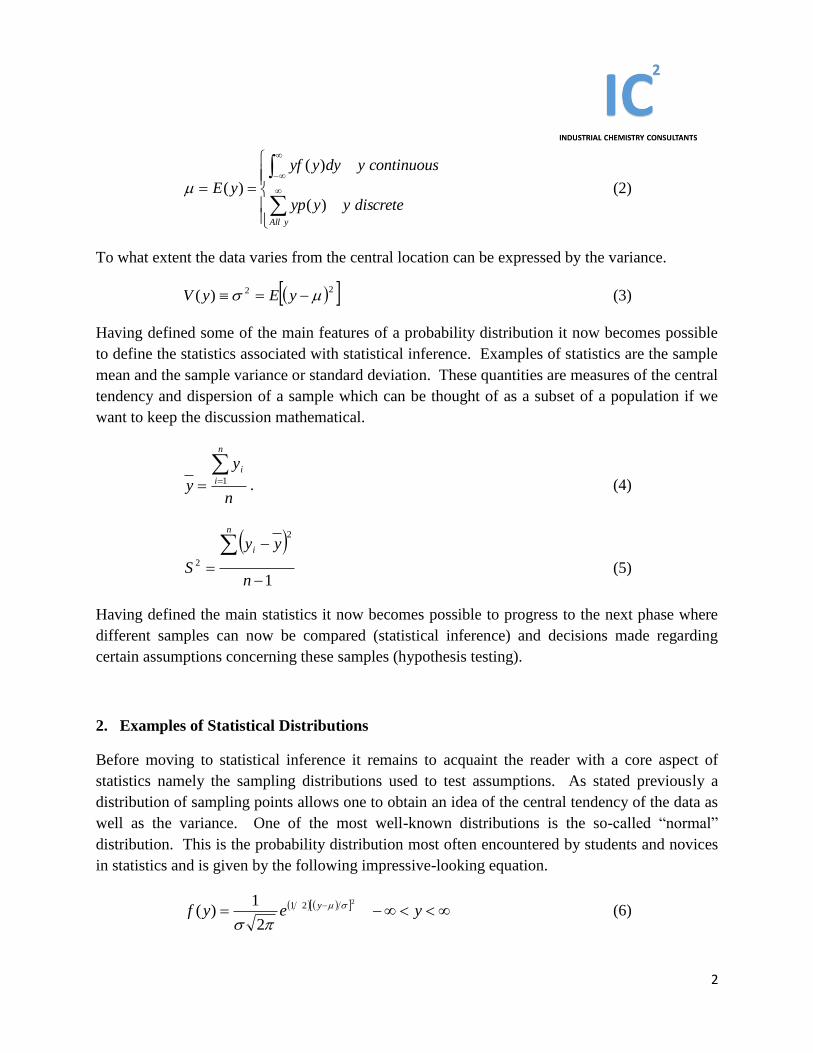
well as the variance. One of the most well-known distributions is the so-called “normal”

distribution. This is the probability distribution most often encountered by students and novices

in statistics and is given by the following impressive-looking equation.

yeyf y2

21

2

1)(

(6)

3

This equation expresses simply what we experience intuitively everyday namely that certain

events or actions produce over a period of time an average value. If we want to look closer at

our results we also see that some values deviate from the average either in a small way or a large

amount.

Figure 1. Characteristic bell shaped curve of normal distribution. The cumulative distribution on the right hand

side is simply the area under the bell curve.

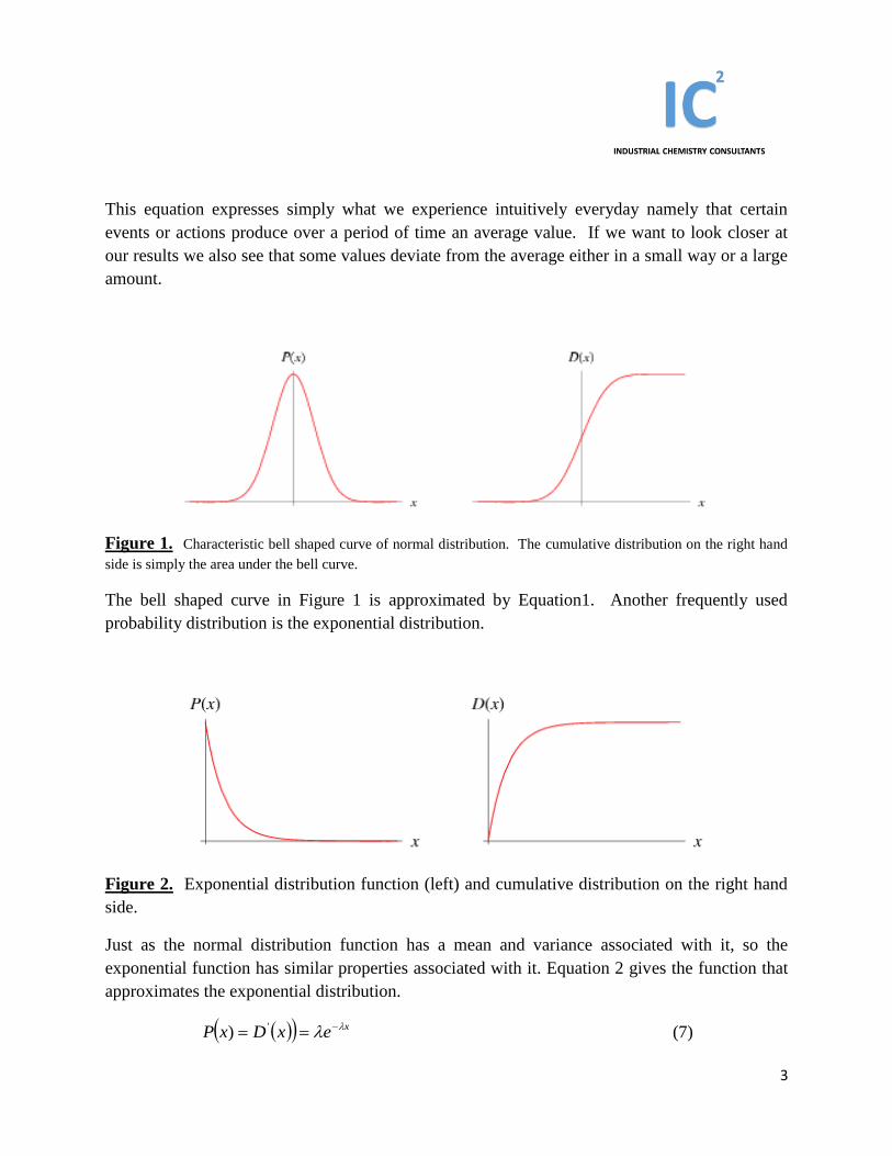
The bell shaped curve in Figure 1 is approximated by Equation1. Another frequently used

probability distribution is the exponential distribution.

Figure 2. Exponential distribution function (left) and cumulative distribution on the right hand

side.

Just as the normal distribution function has a mean and variance associated with it, so the

exponential function has similar properties associated with it. Equation 2 gives the function that

approximates the exponential distribution.

xexDxP ') (7)

4

The mean, variance, skewness and kurtosis are given below.

1 (8)

2

2 1

(9)

21 (10)

62 (11)

The skewness gives an indication to what extent the distribution curve leans to a particular side

while the kurtosis is a measure of the “peakedness” of a distribution. According to one

definition high kurtosis illustrates a distribution with a sharper peak and longer fatter tails while

lower kurtosis indicates a distribution with lower rounder peaks and thinner tails. The normal

distribution has zero kurtosis and skewness and is called mesokurtic.

There are numerous other distributions in use and they have specific areas of application where a

specific type of distribution can describe the observed data. For example, exponential

distributions describe situations such as queuing for example in a bank or supermarket better

than a normal distribution. Because the normal distribution is so well known it is used to

approximate other distributions either in a certain data range or through data transformations.

Sometimes very simple probability distributions can be used if the exact distribution is not

known to obtain an approximate mean or variance. These distributions are the triangular and the

uniform distribution. Figure 3 illustrates the triangular distribution and its cumulative form.

Figure 3. Triangular distribution and its cumulative form on the right hand side.

The function that approximates the triangular distribution is given in Eqation 3 below.

5

bxcforcbab

xb

cxaforacab

ax

xP

))((

)(2

))((

)(2

)( (12)

The mean of the distribution is also given in Equation 13.

cba 3

1 (13)

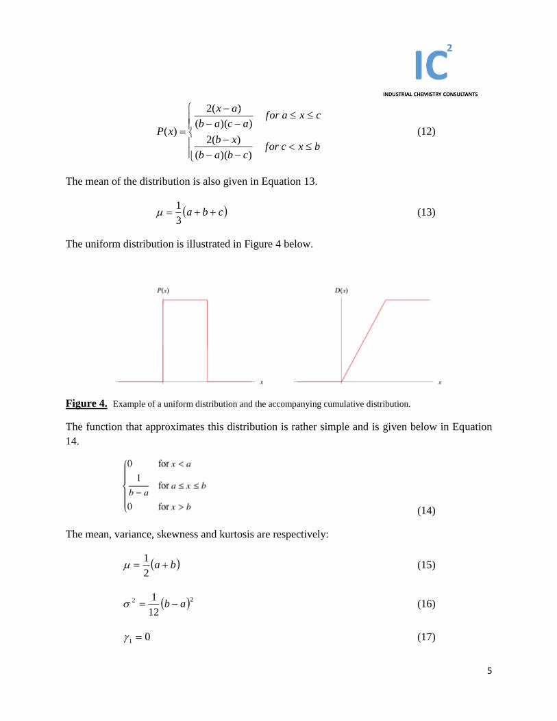
The uniform distribution is illustrated in Figure 4 below.

Figure 4. Example of a uniform distribution and the accompanying cumulative distribution.

The function that approximates this distribution is rather simple and is given below in Equation

14.

(14)

The mean, variance, skewness and kurtosis are respectively:

ba 2

1 (15)

22

12

1ab (16)

01 (17)

6

5

62 (18)

The probability distributions defined up until now are very handy for most work where sample

results have to be compared. Sample comparisons or statistical inference is the backbone of

statistical interpretation of data and as such these distributions are “sampling distributions” that

allows us to analyze the data and to decide whether changes that we make to experimental data

are “real” or significant or simply due to “noise” or random variation. A very important special

case of the normal distribution that allows significant simplification in terms of the mathematics

of the statistical interpretation of data must be introduced at this stage namely the standard

normal distribution. This is the case where μ = 0 and σ2 = 1. Any random variable in a data set

can be transformed so that the data set in its entirety can be described by the standard normal

distribution according to Equation 19 below.

yz (19)

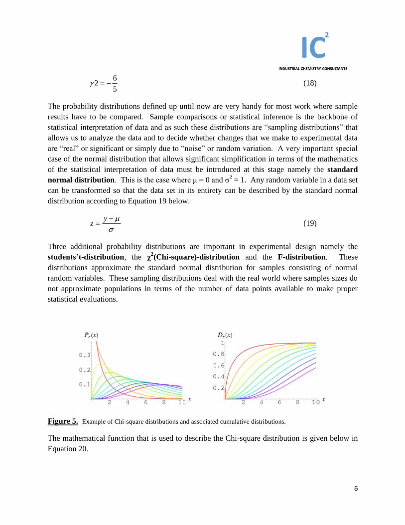
Three additional probability distributions are important in experimental design namely the

students’t-distribution, the χ2(Chi-square)-distribution and the F-distribution. These

distributions approximate the standard normal distribution for samples consisting of normal

random variables. These sampling distributions deal with the real world where samples sizes do

not approximate populations in terms of the number of data points available to make proper

statistical evaluations.

Figure 5. Example of Chi-square distributions and associated cumulative distributions.

The mathematical function that is used to describe the Chi-square distribution is given below in

Equation 20.

7

212

2

22

1)( xk

k

ek

xf

(20)

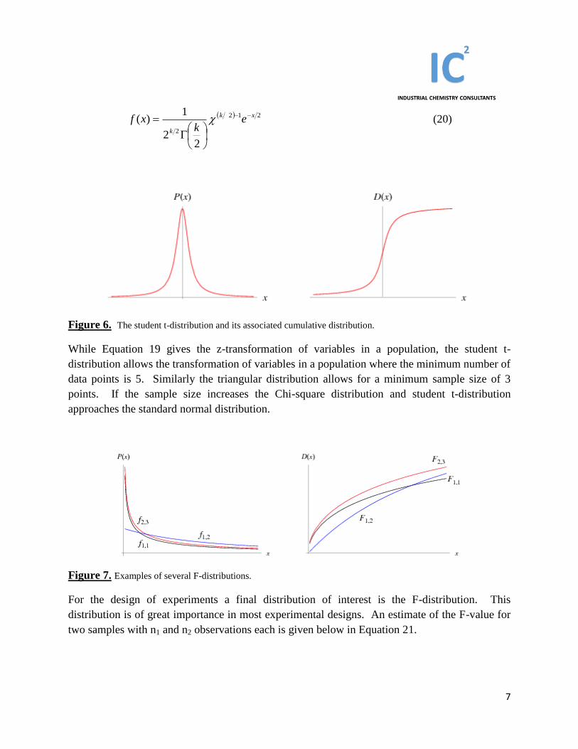
Figure 6. The student t-distribution and its associated cumulative distribution.

While Equation 19 gives the z-transformation of variables in a population, the student t-

distribution allows the transformation of variables in a population where the minimum number of

data points is 5. Similarly the triangular distribution allows for a minimum sample size of 3

points. If the sample size increases the Chi-square distribution and student t-distribution

approaches the standard normal distribution.

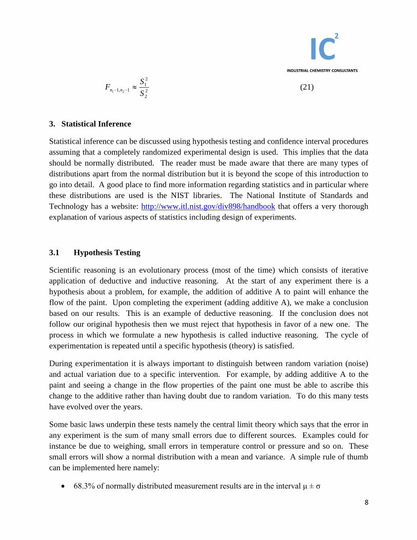
Figure 7. Examples of several F-distributions.

For the design of experiments a final distribution of interest is the F-distribution. This

distribution is of great importance in most experimental designs. An estimate of the F-value for

two samples with n1 and n2 observations each is given below in Equation 21.

8

2

2

2

11,1 21 S

SF nn (21)

3. Statistical Inference

Statistical inference can be discussed using hypothesis testing and confidence interval procedures

assuming that a completely randomized experimental design is used. This implies that the data

should be normally distributed. The reader must be made aware that there are many types of

distributions apart from the normal distribution but it is beyond the scope of this introduction to

go into detail. A good place to find more information regarding statistics and in particular where

these distributions are used is the NIST libraries. The National Institute of Standards and

Technology has a website: http://www.itl.nist.gov/div898/handbook that offers a very thorough

explanation of various aspects of statistics including design of experiments.

3.1 Hypothesis Testing

Scientific reasoning is an evolutionary process (most of the time) which consists of iterative

application of deductive and inductive reasoning. At the start of any experiment there is a

hypothesis about a problem, for example, the addition of additive A to paint will enhance the

flow of the paint. Upon completing the experiment (adding additive A), we make a conclusion

based on our results. This is an example of deductive reasoning. If the conclusion does not

follow our original hypothesis then we must reject that hypothesis in favor of a new one. The

process in which we formulate a new hypothesis is called inductive reasoning. The cycle of

experimentation is repeated until a specific hypothesis (theory) is satisfied.

During experimentation it is always important to distinguish between random variation (noise)

and actual variation due to a specific intervention. For example, by adding additive A to the

paint and seeing a change in the flow properties of the paint one must be able to ascribe this

change to the additive rather than having doubt due to random variation. To do this many tests

have evolved over the years.

Some basic laws underpin these tests namely the central limit theory which says that the error in

any experiment is the sum of many small errors due to different sources. Examples could for

instance be due to weighing, small errors in temperature control or pressure and so on. These

small errors will show a normal distribution with a mean and variance. A simple rule of thumb

can be implemented here namely:

68.3% of normally distributed measurement results are in the interval μ ± σ

9

95.4% of normally distributed measurement results are in the interval μ ± 2σ

99.7% of normally distributed measurement results are in the interval μ ± 3σ

As a consequence if any measured result shows a deviation more than 3σ from the expected

value μ then one should assume that this is due to a measurement error or due to an actual change

brought about by a deliberate change in a variable. To ascertain if it is due to either an error or a

deliberate change involves the use of the aforementioned statistical tests. These tests require the

use of specific distributions as specified previously.

In statistics we always have two hypothesis namely the null hypothesis and the alternative

hypothesis. The null hypothesis assumes that there is no difference between two subjects and

any observed variance is simply due to random noise. The alternative hypothesis can be one

sided or two sided. The two sided alternative is less sensitive and only states that there is a

difference between sample A and sample B. The one sided alternative states that one of the

subjects is better than the other. There is also a risk associated in rejecting the null hypothesis

which is called the level of significance (α) and the erroneous rejection of the null hypothesis is

called a type I error. Therefore a small α signifies a high level of significance. For example, an

α value of 0.05 means that there is a 95% probability that the test statistic can be accepted to

yield accurate results. The power of the experiment is therefore 95% or (1-α). If the null

hypothesis is not rejected when it is false a type II error (β) occurs. Below an example is used to

illustrate some of the statistical tests that are common to experimental design in general.

Sometimes it may be that a practically significant difference (due to experience by the

experimenter) in the data may be observed that does not reflect any statistical significance. This

may indicate that the number of experimental runs may not be enough to confirm the hunch that

the practically significant difference is also statistically significant. The following formula may

then be used to determine the sample size that is required to yield statistically significant results:

2

2/

B

zn

(22)

If a specific power is required for the experiment, say 0.99 then 2 must be 0.005 and from the

standard normal probability tables the z-value can be obtained. The standard deviation may be

approximated by 4/Range . An example taken from the referenced literature (Ref. 13)

should illustrate this important concept.

Example: The assembly time for an electronic component is noted amongst several workers.

The shortest assembly time is 10 minutes while the longest is 22 minutes. How large should the

10

test sample of workers be if the assembly time must be estimated to within 20 seconds at a

confidence level of 99%?

The confidence level is 1-α = 0.99 and therefore the z-value from the standard normal

distribution should be 575.2005.02 zz . The error bound is 20 seconds and the range is 22 –

10 = 12 minutes or 720 seconds. Therefore σ = 720/4 = 180 seconds so that:

08.537

20

180575.22

n

This means about 538 workers should be sampled in order to be sure that a mean is obtained to

within 20 seconds with 99% confidence.

3.2 Two-Sample Student t-Test

The test statistic used to compare two sample means is given below in Equation 23.

21

210

11

nnS

yyt

p

(23)

Where

2

11

21

2

22

2

112

nn

SnSnS p (24)

Note that this is a two-sided test which means it only indicates 21 . A one-sided test would

indicate that 21 or 21 . This is important because a two-sided test requires that half of

α be used. The reference distribution used in this test is the t-distribution previously defined.

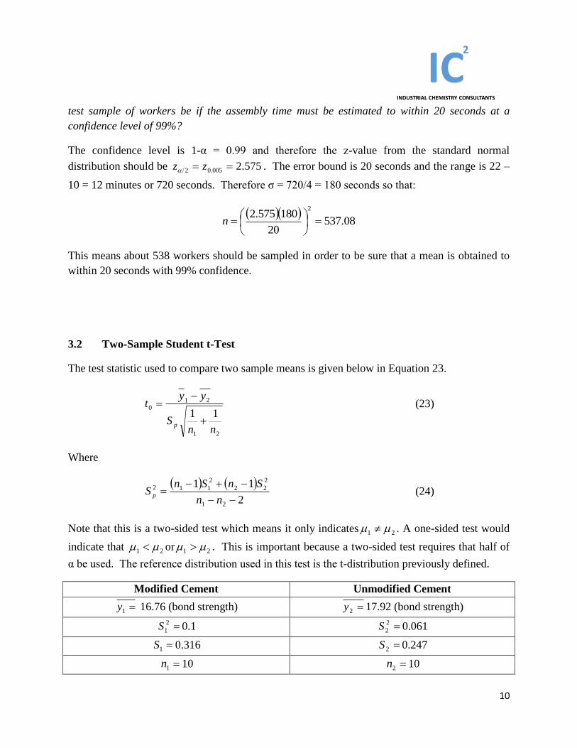
Modified Cement Unmodified Cement

1y 16.76 (bond strength) 2y 17.92 (bond strength)

2

1S 0.1 2

2S 0.061

1S 0.316 2S 0.247

1n 10 2n 10

11

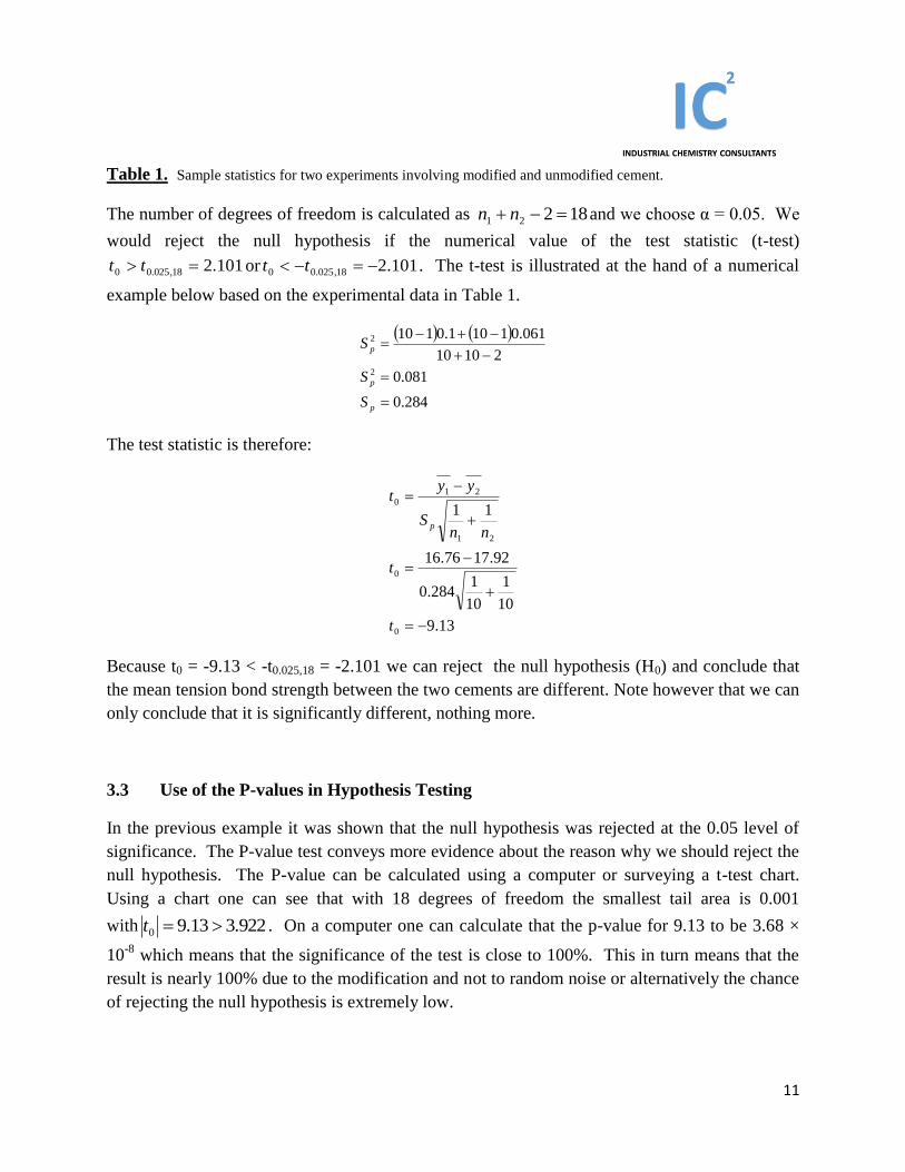
Table 1. Sample statistics for two experiments involving modified and unmodified cement.

The number of degrees of freedom is calculated as 18221 nn and we choose α = 0.05. We

would reject the null hypothesis if the numerical value of the test statistic (t-test)

101.218,025.00 tt or 101.218,025.00 tt . The t-test is illustrated at the hand of a numerical

example below based on the experimental data in Table 1.

284.0

081.0

21010

061.01101.0110

2

2

p

p

p

S

S

S

The test statistic is therefore:

13.9

10

1

10

1284.0

92.1776.16

11

0

0

21

210

t

t

nnS

yyt

p

Because t0 = -9.13 < -t0.025,18 = -2.101 we can reject the null hypothesis (H0) and conclude that

the mean tension bond strength between the two cements are different. Note however that we can

only conclude that it is significantly different, nothing more.

3.3 Use of the P-values in Hypothesis Testing

In the previous example it was shown that the null hypothesis was rejected at the 0.05 level of

significance. The P-value test conveys more evidence about the reason why we should reject the

null hypothesis. The P-value can be calculated using a computer or surveying a t-test chart.

Using a chart one can see that with 18 degrees of freedom the smallest tail area is 0.001

with 922.313.90 t . On a computer one can calculate that the p-value for 9.13 to be 3.68 ×

10-8

which means that the significance of the test is close to 100%. This in turn means that the

result is nearly 100% due to the modification and not to random noise or alternatively the chance

of rejecting the null hypothesis is extremely low.

12

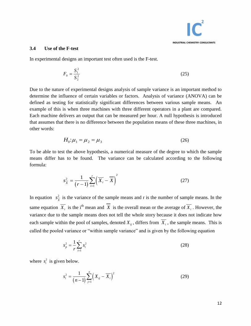
3.4 Use of the F-test

In experimental designs an important test often used is the F-test.

2

2

2

10

S

SF (25)

Due to the nature of experimental designs analysis of sample variance is an important method to

determine the influence of certain variables or factors. Analysis of variance (ANOVA) can be

defined as testing for statistically significant differences between various sample means. An

example of this is when three machines with three different operators in a plant are compared.

Each machine delivers an output that can be measured per hour. A null hypothesis is introduced

that assumes that there is no difference between the population means of these three machines, in

other words:

H0 1 2 3: (26)

To be able to test the above hypothesis, a numerical measure of the degree to which the sample

means differ has to be found. The variance can be calculated according to the following

formula:

sr

X XX i

i

r2

1

21

1

(27)

In equation sX

2 is the variance of the sample means and r is the number of sample means. In the

same equation X i is the ith

mean and X is the overall mean or the average of X i . However, the

variance due to the sample means does not tell the whole story because it does not indicate how

each sample within the pool of samples, denoted X ij , differs from X i , the sample means. This is

called the pooled variance or “within sample variance” and is given by the following equation

sr

sp i

i

r2 2

1

1

(28)

where si

2 is given below.

s

nX Xi ij i

j

n2

2

1

1

1

(29)

13

So, what does this mean? This analysis strives to tell us whether the sample means are truly just

chance variations about a common population mean, i.e. the null hypothesis holds or the null

hypothesis is wrong and there is some erratic behavior within the samples. This would mean that

the data is not spread by chance around a general population mean and there is some significant

effect due to some machine (in this illustration).

If H0 is true, the F-ratio will have a value near 1. However, because of statistical fluctuation

(we assume the data is normally distributed), F sometimes will be above 1 or sometimes below 1.

If H0 is not true, ns

X

2 will be relatively large compared to sp

2 and the F-ratio will be much

greater than 1. This brings us to a convenient method of establishing quickly whether a specific

factor is significant. We simply look at the analysis of variance table and the concomitant F-

ratios. However, although they provide a point of departure in evaluating data, these F-ratios on

their own do not tell us enough. We still need to test the null hypothesis and decide whether to

reject the null-hypothesis or not because we do not know the degree of fluctuation in the data

around the F-values.

The F-ratios or values can be evaluated at various levels of probabilities using F-tables. If the

calculated F-ratio value is compared with the value in the F-table, the probability of accepting

the null-hypothesis can be evaluated. If the calculated F-ratio value is much larger than the value

in the F-table at a particular probability level, the null-hypothesis may be rejected at that level.

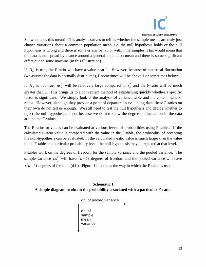
F-tables work on the degrees of freedom for the sample variance and the pooled variance. The

sample variance nsX

2 will have n 1 degrees of freedom and the pooled variance will have

r n 1 degrees of freedom (d.f.). Figure 1 illustrates the way in which the F-table is used.1

Schematic 1

A simple diagram to obtain the probability associated with a particular F-ratio.

d.f. of pooled variance

d.f. of sample mean variance

14

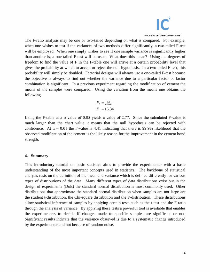
The F-ratio analysis may be one or two-tailed depending on what is compared. For example,

when one wishes to test if the variances of two methods differ significantly, a two-tailed F-test

will be employed. When one simply wishes to see if one sample variance is significantly higher

than another is, a one-tailed F-test will be used. What does this mean? Using the degrees of

freedom to find the value of F in the F-table one will arrive at a certain probability level that

gives the probability at which to accept or reject the null-hypothesis. In a two-tailed F-test, this

probability will simply be doubled. Factorial designs will always use a one-tailed F-test because

the objective is always to find out whether the variance due to a particular factor or factor

combination is significant. In a previous experiment regarding the modification of cement the

means of the samples were compared. Using the variation from the means one obtains the

following.

34.160

0061.01.0

0

F

F

Using the F-table at a α value of 0.05 yields a value of 2.77. Since the calculated F-value is

much larger than the chart value it means that the null hypothesis can be rejected with

confidence. At α = 0.01 the F-value is 4.41 indicating that there is 99.9% likelihood that the

observed modification of the cement is the likely reason for the improvement in the cement bond

strength.

4. Summary

This introductory tutorial on basic statistics aims to provide the experimenter with a basic

understanding of the most important concepts used in statistics. The backbone of statistical

analysis rests on the definition of the mean and variance which is defined differently for various

types of distributions of the data. Many different types of data distributions exist but in the

design of experiments (DoE) the standard normal distribution is most commonly used. Other

distributions that approximate the standard normal distribution when samples are not large are

the student t-distribution, the Chi-square distribution and the F-distribution. These distributions

allow statistical inference of samples by applying certain tests such as the t-test and the F-ratio

through the analysis of variance. By applying these tests a powerful tool is available that enables

the experimenters to decide if changes made to specific samples are significant or not.

Significant results indicate that the variance observed is due to a systematic change introduced

by the experimenter and not because of random noise.

15

REFERENCES

1. Chemometrics: Experimental Design, Analytical Chemistry by OpenLearning, Ed

Morgan, John Wiley and Sons, New York, (1982)

2. Designing for Quality, An Introduction to the best of Taguchi and Western methods

of Statistical Experimental Design, Robert H. Lochner, Joseph E. Matar, Quality

Resources, A Division of The Kraus Organisation Limited, New York, (1990)

3. Statistics and Experimental Design in Engineering and the Physical Sciences,

Volume II, Second Edition, Norman L. Johnson, Fred C. Leone, John Wiley & Sons,

New York, (1977)

4. Experiments with Mixtures, Designs, Models, and the analysis of Mixture data, John

A. Cornell, John Wiley & Sons, New York, (1981)

16

5. Introductory Statistics, Third Edition, Thomas H. Wonnacot, Ronald J. Wonnacot, John

Wiley & Sons, New York, (1977)

6. Edward J. Powers, Proceedings of the Water-Borne and Higher Solids Coatings

Symposium, “Handling and curing a water-borne epoxy coating”, pp. 111 – 135,

(1981)

7. Chorng-Shyan Chern, Yu-Chang Chen, Polymer Journal, “Semibatch emulsion

polymerization of butyl acrylate stabilised by a polymerizable surfactant”, , Vol. 28, No.

7, pp. 627-632, (1996)

8. G.E.P. Box, J.S. Hunter, Technometrics, “The 2k-p

fractional factorial designs. Part I”,

Vol. 3, No. 3, (1961)

9. W.J. Youden, Technometrics, “Partial confounding in fractional replication”, Vol. 3,

No. 3, (1961)

10. Dunae E. Long Analytica Chimica Acta, “Simplex optimisation of the response from

chemical systems”, Vol. 46, pp. 193 – 206, (1969)

11. Linear Algebra and its Applications, Gilbert Strang, Third Edition, Chapter 3, p. 153,

Harcourt Brace Jovanovich, Inc., Orlando, (1988)

12. Andre I. Khuri, John A. Cornell, Response Surfaces, Designs and Analyses, Second

Edition, Revised and Expanded, Chapter 2, Matrix Algebra, Least Squares, the Analysis

of Variance, and Principles of Experimental Design, Marcel Dekker, Inc., New York,

1996

13. Statistics for Management and Economics, Gerald Keller, Brian Warrack, Duxbury

Press, Johannesburg, 1997

14. Introduction to DOE, Veli-Matti Taavitsainen, 2009

15. Design and Analysis of Experiments, 5th

Edition, Douglas C. Montgomery, Wiley

Student Edition, Wiley India, 2004

16. Design and optimization in organic synthesis, Second revised and enlarged edition,

Rolf Carlson, Johan E. Carlson, Elsevier, Sweden, 2005

17. Operations Research: Applications and Algorithms, Wayne L. Winston, PWS-Kent

Publishing Company, Boston, 1987

17

18. http://mathworld.wolfram.com/NormalDistribution.html