introduction to fiber optic sensors -...

Chapter I

Introduction to Fiber Optic Sensors

1.1 Introduction

An optical fiber is defined as a flexible optically transparent

fiber, usually made of glass or plastic, through which light can be transmitted

by successive internal reflections. The history of light guidance starts with

the experiment by Daniel Colladon and Jacques Babinet in 1841 [1]. In their

experiment they demonstrated that a jet of water can guide light waves

through it. John Tyndall included a demonstration of it in his public lectures

and also wrote about the property of total internal reflection in an

introductory book about the nature of light in 1870. During the early half of

20th century, experiments were carried out using bent glass rod to guide light

but leakage of optical power was the hurdle. The solution to this problem

was solved by Brian O’Brien, Haay Hopkins and Narinder Kapany in 1950

by proposing a lower refractive index coating termed as cladding to the

waveguide [1]. The serious problem faced during that period was related to

the absorption of light by glass and the attenuation in glass fibers was around

1000 dB/Km.

In 1965 Charles K Kao and George Hockham concluded that the loss

in optical fibers is merely due to absorption by impurities and the

fundamental limitation for glass light attenuation is below 20 dB/km, which

is a key threshold value for optical communications [2]. This conclusion

opened an intense race to find low-loss materials and suitable fibers for

reaching such criteria which laid the groundwork for high-speed data

communication in the Information Age. In 2009 The Royal Swedish

Academy of Sciences awarded the Nobel Prize in Physics to Charles K Kao

"for groundbreaking achievements concerning the transmission of light in

fibers for optical communication"[3]. The fiber loss gradually got reduced

and in 1970 Corning introduced the 20 dB/Km loss fiber making the optical

fibers usable for communication purpose. The first generation optical

communication used 850 nm light with a loss of 22dB/Km which then

migrated to second generation where 1310 nm was used with 0.5dB/Km loss.

Now we are in the third generation fiber optic communication where 1550


2

nm wavelength is used with loss in the range of 0.2 dB/Km, which is close to

the theoretical limit based on Rayleigh scattering in an amorphous glass

material [4]. Optical fibers provide unmatched transmission bandwidth, but

light propagates 31% slower in a silica glass fiber than in vacuum. Wide-

bandwidth signal transmission with low latency is emerging as a key

requirement in a number of applications, including the development of future

exascale supercomputers, financial algorithmic trading and cloud computing.

The research today is focused on the development of hollow-core photonic-

bandgap fibers which can significantly reduce fiber latency due to air

guidance. Recently a fundamentally improved hollow-core photonic-

bandgap fiber that provides a loss of 3.5 dB km−1 with a wide bandwidth of

160 nm was reported to transmit 37 × 40 Gbit s−1 channels at a 1.54 µs

km−1 faster speed than a conventional fiber [5].

The field of fiber optic technologies has undergone tremendous

growth and advancement and has revolutionized the telecommunications

industry by providing high performance and reliable telecommunication

links. The costs of laser diodes and optical fibers have drastically reduced

along with the evolution of the technology. In parallel with these

developments, fiber optic sensor [6-10] technology has undergone

tremendous growth using the technologies associated with the optoelectronic

and fiber optic communications industry. Over the past decades fiber optic

sensors for the measurement of strain [11], temperature [12], pressure [13],

velocity [14,15], magnetic field [16], electric current [17], acoustic signal

[18] chemical and biological parameters[19-22]etc. have been reported.

Though fiber optic sensors excel in performance, they face the problem of

competing with the well-established conventional sensor technologies which

provide adequate and reliable performance at low cost. However they have

found excellent applications in harsh environment defined by high

temperature, high pressure, corrosive/erosive, and strong electromagnetic

interference, where conventional electronic sensors do not have a chance to

survive. In some applications the ability to efficiently multiplex fiber sensors

may be the criterion used to select fiber sensors over other technologies.

Fiber Optic sensors have inherent advantages such as immunity to

electromagnetic interference (EMI), lightweight, small size, high sensitivity,

multiplexing capability and large bandwidth over other technologies. Due to

these inherent advantages fiber optic sensors have an edge over electronic


3

sensors and various ideas have been proposed and various techniques have

been developed for various measurands and applications. A vide variety of

sensors were reported during the past decades for sensing various physical

and chemical parameters. Though some types of optical fiber sensors have

been commercialized, only a limited number of techniques and applications

have been commercially successful.

This chapter describes the structure and light guiding mechanism of

optical fibers. The general principle of operation of fiber optic sensors is

discussed. Various schemes used in fiber optic sensing technology to convert

the measuring parameter into corresponding variation of optical properties

are presented along with their merits and demerits. This chapter also presents

a brief review about fiber optic sensors reported during the past decades in

the area of quality evaluation.

1.2. Optical Fiber

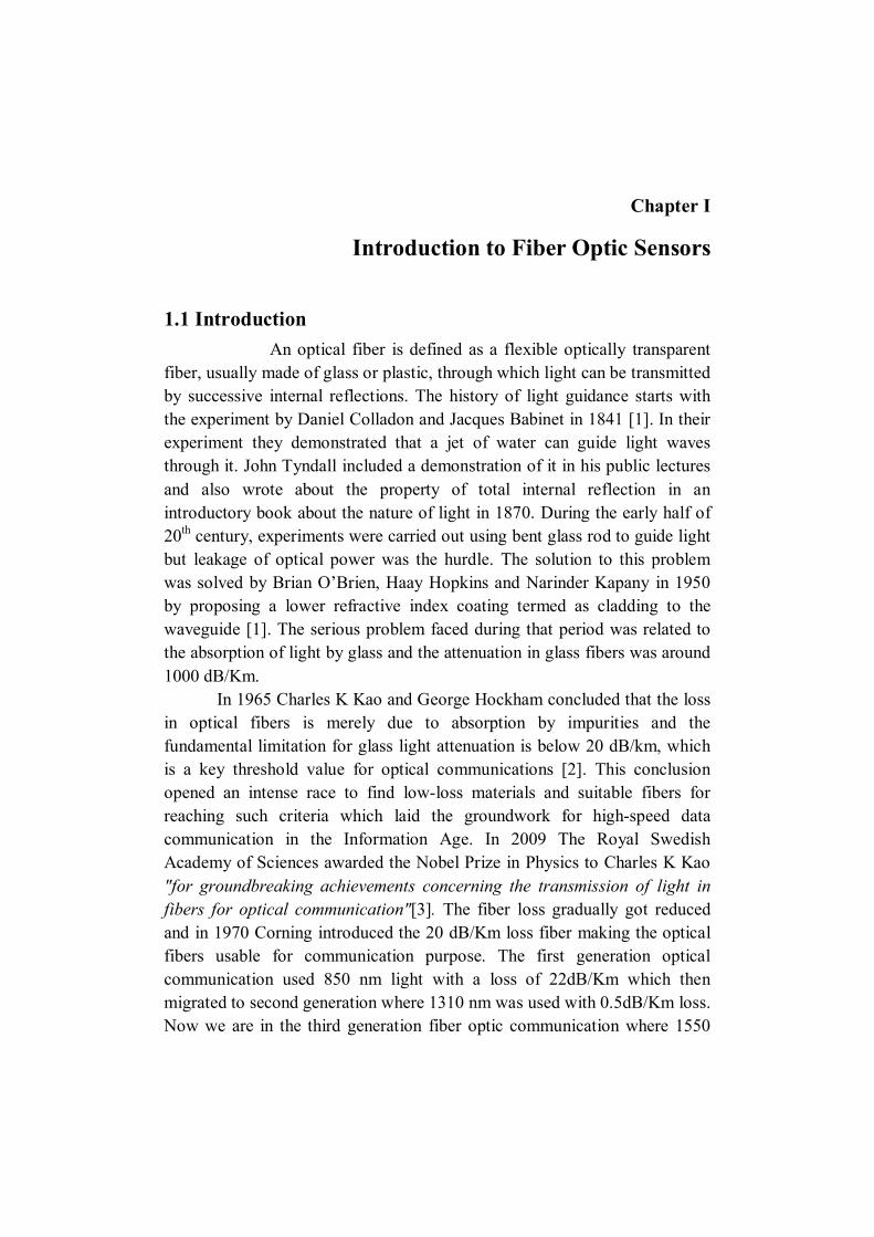
A typical communication optical fiber is a cylindrical optical

waveguide as shown in figure 1.1(a), consisting of a number of layers

namely core, cladding, buffer and jacket. The outer layers, typically made of

polymer or plastic materials, are the buffer and jacket and are for the purpose

of reinforcing the mechanical strength. The center layer is made of doped

glass and is the core of the fiber where most of the light energy is confined.

The cladding layer is made of fused silica glass and has a refractive index

(ncl) less than that of the core (nco). Thus light is guided inside the core as a

result of total internal reflection (TIR) at the core-cladding interface [23,24].

Figure 1.1 a) Structure of Optical Fiber b) Ray-optics representation of light propagation mechanisms in an ideal step-index optical fiber


4

If a beam of light is incident on the end face of a fiber within the

angular cone specified by an entrance (or acceptance) angle θ0, the light is

confined to the core material by virtue of total internal reflection from the

core-cladding interface [24], as shown in Figure 1.1(b). From elementary

optics, total internal reflection is only supported in the fiber if the angle that

the ray makes with the core-cladding interface is greater than the critical

angle θc. By applying Snell’s law to the air-fiber face boundary, the

maximum entrance angle θ0 can be deduced as

220sin clco nnn (1.1)

where n is the refractive index of air.

The value on the left hand side of equation 1.1 is defined as the

numerical aperture (NA) of the fiber. Since it is related to the maximum

acceptance angle, numerical aperture defines the light gathering capability of

the fiber.

Thus 22clco nnNA (1.2)

1.2.1 Mechanism of Light Guidance and Fiber Modes

The basic mechanism by which light is transmitted through an optical

fiber is total internal reflection (TIR). The simplest approach in analyzing

light confinement is using geometrical optics. When a light ray incidents on

the boundary of an optically denser medium (refractive index nco) that

separates it from a rarer medium (refractive index ncl, nco>ncl) at an angle

greater than the critical angle (θc) it will be totally internally reflected back to

the denser medium itself. Thus light coupled to the core gets confined in it

due to total internal reflection at the core cladding boundary.

Although it would seem possible for all light rays to propagate along

the fiber if they are incident at an angle θ1 (π/2-angle of incidence θ) from

the core-cladding interface, where θ1< θc , this is not the case because the

phase of the light wave also needs to be considered [24]. The phase that

results after the wave has undergone two reflections from the core-cladding

interface must be an integer multiple of the incident phase. If this condition

is not satisfied, the wave will interfere destructively with itself and ultimately

cease to propagate, thus restricting the light to certain discrete ray paths

within the core. The total phase shift consists of two components namely the


5

shift in phase due to the distance traversed by the light wave and the Goos-

Hanchen shift due to reflection from the dielectric (core-cladding) interface

[23,24].

The phase change due to the former effect can be formulated from

Skco (1.3)

where kco is the propogation constant in the medium of refractive index nco

and S is the distance the wave travels in the material.

Since the free space propagation constant k=kco/nco=2π/λ

/2 SnkSn coco (1.4)

The Goos-Hanchen shift arising from a single reflection is calculated using

the following expression [24]

sin

costan2

22

1

cl

clco

HGn

nn

(1.5)

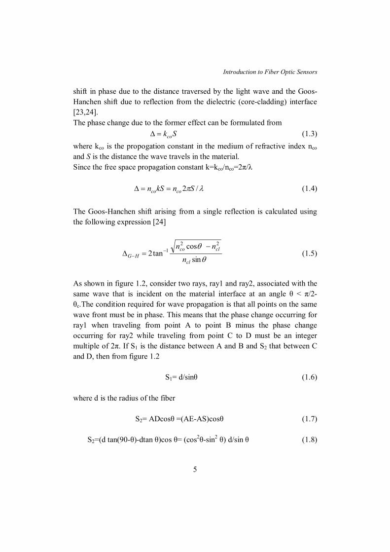
As shown in figure 1.2, consider two rays, ray1 and ray2, associated with the

same wave that is incident on the material interface at an angle θ < π/2-

θc.The condition required for wave propagation is that all points on the same

wave front must be in phase. This means that the phase change occurring for

ray1 when traveling from point A to point B minus the phase change

occurring for ray2 while traveling from point C to D must be an integer

multiple of 2π. If S1 is the distance between A and B and S2 that between C

and D, then from figure 1.2

S1= d/sinθ (1.6)

where d is the radius of the fiber

S2= ADcosθ =(AE-AS)cosθ (1.7)

S2=(d tan(90-θ)-dtan θ)cos θ= (cos2θ-sin2 θ) d/sin θ (1.8)


6

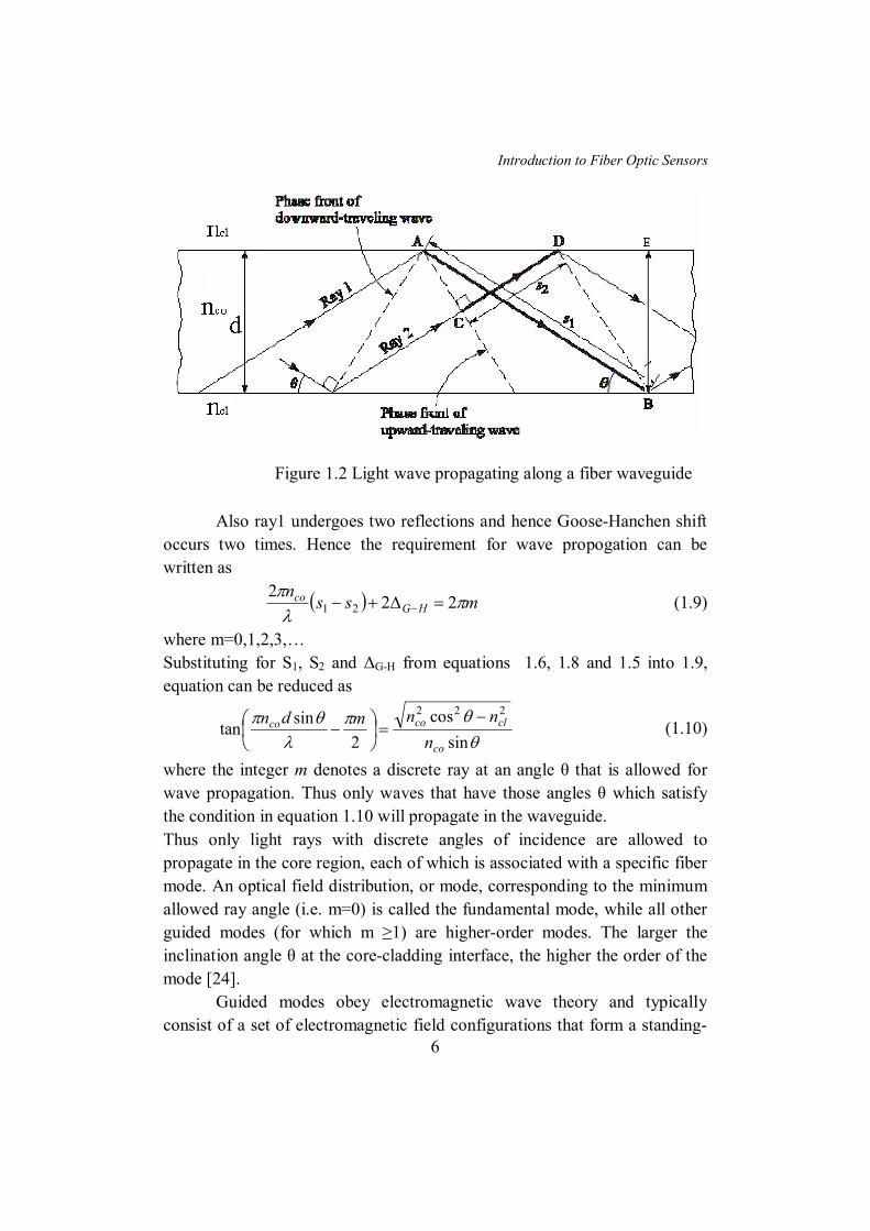
Also ray1 undergoes two reflections and hence Goose-Hanchen shift

occurs two times. Hence the requirement for wave propogation can be

written as

mssn

HGco

22

221 (1.9)

where m=0,1,2,3,…

Substituting for S1, S2 and ΔG-H from equations 1.6, 1.8 and 1.5 into 1.9,

equation can be reduced as

sin

cos

2

sintan

222

co

clcoco

n

nnmdn

(1.10)

where the integer m denotes a discrete ray at an angle θ that is allowed for

wave propagation. Thus only waves that have those angles θ which satisfy

the condition in equation 1.10 will propagate in the waveguide.

Thus only light rays with discrete angles of incidence are allowed to

propagate in the core region, each of which is associated with a specific fiber

mode. An optical field distribution, or mode, corresponding to the minimum

allowed ray angle (i.e. m=0) is called the fundamental mode, while all other

guided modes (for which m ≥1) are higher-order modes. The larger the

inclination angle θ at the core-cladding interface, the higher the order of the

mode [24].

Guided modes obey electromagnetic wave theory and typically

consist of a set of electromagnetic field configurations that form a standing-

Figure 1.2 Light wave propagating along a fiber waveguide


7

wave pattern in a direction transverse to that of the fiber axis. Maxwell’s

equations in a linear, isotropic dielectric material having no currents and free

charges are given below.

0. D (1.11)

0. B (1.12)

t

BE

(1.13)

t

DH

(1.14)

where ε is the permittivity and μ is the permeability of the medium. The

electric flux and magnetic flux are given by D=εE and B=μH

By taking the curl of these equations, the wave equations for the

electromagnetic fields are obtained as

2

22

t

EE

(1.15)

2

22

t

HH

(1.16)

Here 2 is called the scalar Laplacian and the choice of coordinate system is

critical in solving the wave equation. If a cylindrical coordinate system

{r,ф,z} with the z axis lying on the axis of the wave guide is defined for a

cylindrical fiber, then the solutions of the wave equations take the form

ztjerEE ,0 (1.17)

ztjerHH ,0 (1.18)

which are harmonic in time t and coordinate z. The parameter β is the z

component of the propagating mode while E and H gives the electric and

magnetic filed distributions of the mode.

As discussed using ray theory, the electric field distribution has a

peak value corresponding to points where two positive wave fronts interfere

constructively, and a trough is formed for constructive interference between

negative phase fronts [23]. Destructive interference occurs when positive and

negative phase fronts cause total field cancellation at a certain point. Thus a

standing wave is formed in the transverse direction that varies periodically

along the fiber’s axis. This standing wave has a period corresponding to the

wavelength given by [23]


8

2

cos0

con (1.19)

Fiber modes traveling in the positive z-direction, composed of light of a

single angular frequency ω (and wavelengthλ), have a spatial and time

dependence proportional to ej(ωt-βz) . The fiber optic axial propagation

constant β– the component of k in the z direction is given by [24]

coscokn (1.20)

Due to the restriction on the inclination angle θ, the propagation constant β

also has a discrete set of solutions, and is denoted as an eigenvalue. This

constant is thus an indication of whether or not the mode propagates in the

core of the fiber or not. A mode remains guided if [24]

cocl knkn (1.21)

The wave equations in cylindrical coordinates are obtained by substituting

the general solution in the wave equations. The equations thus obtained are

011 2

2

2

22

2

z

zzz EqE

rr

E

rr

E

(1.22)

011 2

2

2

22

2

z

zzz HqH

rr

H

rr

H

(1.23)

where 22222 kq

These two equations contain either Ez or Hz. This implies that the

longitudinal components of E and H are uncoupled and can be chosen

arbitrarily provided that they satisfy equations 1.22 and 1.23. However,

coupling of Ez and Hz is required by the boundary conditions of the

electromagnetic field components. If there is no coupling then mode

solutions can be obtained in which either Ez or Hz = 0.When Ez = 0 modes

are called transverse electric or TE modes and when Hz = 0, they are called

transverse magnetic or TM modes. Hybrid modes exist if both Ez and Hz are

non zeros and are designated as HE or EH modes depending whether Hz or

Ez makes a larger contribution to the transverse field. The two lowest order

modes are designated by HE11 and TE01.

The wave equations can be solved using the variable separable method. The

solution of the equation is of the form [24]

tFzFFrAFEz 4321 (1.24)


9

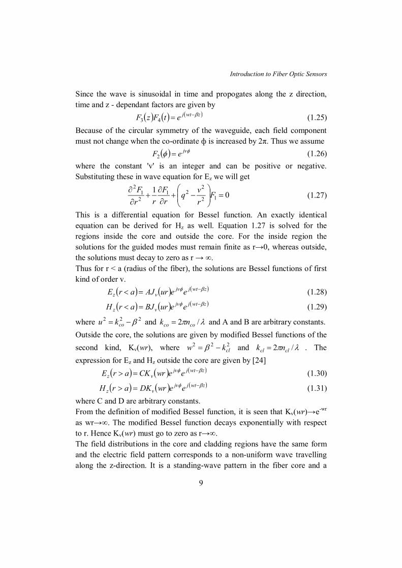
Since the wave is sinusoidal in time and propogates along the z direction,

time and z - dependant factors are given by

zwtjetFzF 43 (1.25)

Because of the circular symmetry of the waveguide, each field component

must not change when the co-ordinate ф is increased by 2π. Thus we assume

jveF 2 (1.26)

where the constant 'v' is an integer and can be positive or negative.

Substituting these in wave equation for Ez we will get

01

12

221

21

2

F

r

vq

r

F

rr

F (1.27)

This is a differential equation for Bessel function. An exactly identical

equation can be derived for Hz as well. Equation 1.27 is solved for the

regions inside the core and outside the core. For the inside region the

solutions for the guided modes must remain finite as r→0, whereas outside,

the solutions must decay to zero as r → ∞.

Thus for r < a (radius of the fiber), the solutions are Bessel functions of first

kind of order v.

zwtjjvvz eeurAJarE (1.28)

zwtjjvvz eeurBJarH (1.29)

where 222 coku and /2 coco nk and A and B are arbitrary constants.

Outside the core, the solutions are given by modified Bessel functions of the

second kind, Kv(wr), where 222clkw and /2 clcl nk . The

expression for Ez and Hz outside the core are given by [24]

zwtjjvvz eewrCKarE (1.30)

zwtjjvvz eewrDKarH (1.31)

where C and D are arbitrary constants.

From the definition of modified Bessel function, it is seen that Kv(wr)→e-wr

as wr→∞. The modified Bessel function decays exponentially with respect

to r. Hence Kv(wr) must go to zero as r→∞.

The field distributions in the core and cladding regions have the same form

and the electric field pattern corresponds to a non-uniform wave travelling

along the z-direction. It is a standing-wave pattern in the fiber core and a


10

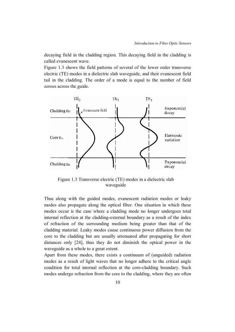
decaying field in the cladding region. This decaying field in the cladding is

called evanescent wave.

Figure 1.3 shows the field patterns of several of the lower order transverse

electric (TE) modes in a dielectric slab waveguide, and their evanescent field

tail in the cladding. The order of a mode is equal to the number of field

zeroes across the guide.

Thus along with the guided modes, evanescent radiation modes or leaky

modes also propagate along the optical fiber. One situation in which these

modes occur is the case where a cladding mode no longer undergoes total

internal reflection at the cladding-external boundary as a result of the index

of refraction of the surrounding medium being greater than that of the

cladding material. Leaky modes cause continuous power diffusion from the

core to the cladding but are usually attenuated after propagating for short

distances only [24], thus they do not diminish the optical power in the

waveguide as a whole to a great extent.

Apart from these modes, there exists a continuum of (unguided) radiation

modes as a result of light waves that no longer adhere to the critical angle

condition for total internal reflection at the core-cladding boundary. Such

modes undergo refraction from the core to the cladding, where they are often

Figure 1.3 Transverse electric (TE) modes in a dielectric slab waveguide


11

trapped as a result of the abrupt cladding-ambient interface to form cladding

modes. Once generated, cladding modes travel alongside the guided core

modes in the optical fiber. Subsequently, mode coupling occurs because the

electric field distributions of both types of modes penetrate the material on

either side of the core-cladding interface. This mainly results in power being

lost from the guided core modes into the cladding. A lossy coating around

the cladding serves to attenuate cladding modes, thus limiting the amount of

optical power leaking out of the core.

1.2.2 Weakly guiding approximation and Linearly Polarized (LP) modes

The electromagnetic field expressions for the guided modes are rather

complicated to derive and hence a simpler method for obtaining the fiber

modes is required. An assumption is made that will simplify analysis to a

great extent – the weakly guiding fiber approximation [24], first introduced

by Gloge in 1971 [25]. This approximation technique assumes that the

difference in refractive index between the core of the fiber and cladding

material is very small, typically of the order of one percent (nco-ncl <<1) .

Technically speaking, the weakly guiding approximation neglects the

longitudinal components of the electric and magnetic fields , resulting in

linearly polarised (LP) ‘pseudo-modes’ [24]. This terminology has been

applied because the waves described by these simplified solutions propagate

at small angles to the fiber axis and are essentially polarised in a single

direction, transverse to the fiber axis. In this scheme for the lowest order

modes, each LP0m mode is derived from an HE1m mode and each LP1m mode

comes from TE0m, TM0m, and HE0m modes. Thus the fundamental LP01 mode

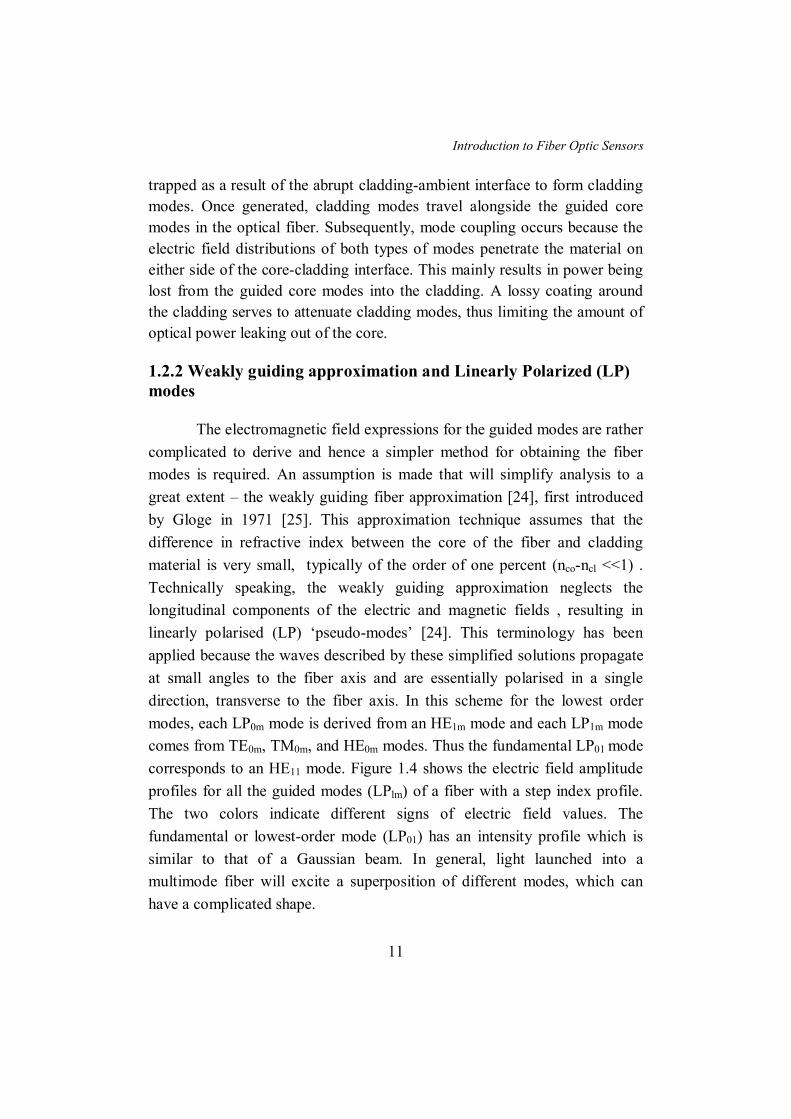
corresponds to an HE11 mode. Figure 1.4 shows the electric field amplitude

profiles for all the guided modes (LPlm) of a fiber with a step index profile.

The two colors indicate different signs of electric field values. The

fundamental or lowest-order mode (LP01) has an intensity profile which is

similar to that of a Gaussian beam. In general, light launched into a

multimode fiber will excite a superposition of different modes, which can

have a complicated shape.


12

1.2.3. Single mode fiber and Normalized frequency

A core mode remains guided as long as β satisfies the condition given

in equation 1.21. The boundary between truly guided modes and leaky

modes is defined by the cutoff condition β=nclk. Another parameter

connected with the cutoff condition is called the normalized frequency or V

parameter/number defined by [24]

NAa

nna

V clco

22 22 (1.32)

where a is the radius of the fiber core

This is a dimensionless number that determines how many modes a fiber can

support. Except for the fundamental or lowest order mode (LP01) each mode

can exist only for values of V that exceed a certain limiting value. The

modes are cutoff when β=nclk, and this occurs when V≤2.405. The

fundamental mode has no cutoff and ceases to exist only when the core

diameter is zero. This is the principle on which single mode fibers are

Figure 1.4 Electric field amplitude profiles for the guided modes (LPlm) of a step index fiber


13

constructed, which guides only the fundamental mode. As per equation 1.32,

V parameter can be reduced by reducing numerical aperture (NA) and/or

radius of the core ‘a’. Single mode fibers are fabricated by letting the core

diameter to be a few wavelengths (usually 8-12 μm) and by having small

index differences between the core and the cladding.

The V number can also be used to calculate the number of modes M in a

multimode fiber and is given by [24]

M=V2/2 (1.33)

1.3. Fiber Optic Sensors

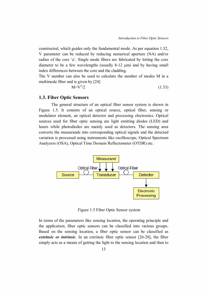
The general structure of an optical fiber sensor system is shown in

Figure 1.5. It consists of an optical source, optical fiber, sensing or

modulator element, an optical detector and processing electronics. Optical

sources used for fiber optic sensing are light emitting diodes (LED) and

lasers while photodiodes are mainly used as detectors. The sensing area

converts the measurands into corresponding optical signals and the detected

variation is processed using instruments like oscilloscope, Optical Spectrum

Analyzers (OSA), Optical Time Domain Reflectometer (OTDR) etc.

In terms of the parameters like sensing location, the operating principle and

the application, fiber optic sensors can be classified into various groups.

Based on the sensing location, a fiber optic sensor can be classified as

extrinsic or intrinsic. In an extrinsic fiber optic sensor [26-28], the fiber

simply acts as a means of getting the light to the sensing location and then to

Figure 1.5 Fiber Optic Sensor system


14

the detector. In the sensing zone the properties of light is changed using

various physical and chemical techniques. Chemical agents like dyes can be

used to change of the properties of the light in the presence of measurands or

a physical deformation proportional to the measurands can change the

coupled light intensity.

In the case of intrinsic fiber optic sensors, the internal property of optical

fiber itself converts the environmental changes into a modulated light signal.

This modulation of light signal can be in the form of intensity, phase,

frequency or polarization [6-10, 26].

Based on the operating principle or the light modulation process, a fiber

optic sensor can be classified as intensity, phase, frequency, or polarization

modulated sensor [6-10]. All these parameters can be transformed as

functions of external perturbations. The external perturbations can be sensed

by measuring these parameters and their changes.

1.3.1 Intensity modulated Fiber Optic Sensors

Intensity-based fiber optic sensors rely on generating a loss or gain to

the transmitted optical power proportional to the measurands. They are made

by using a transducer to convert the measurand into a factor which causes

attenuation of the signal. There are a variety of mechanisms like

microbending loss, attenuation and evanescent fields to produce a change in

the optical intensity guided by an optical fiber proportional to the

measurand[6- 10]. These types of fiber optic sensors possess inherent

advantages like simplicity of implementation, low cost, multiplexing

capability, and ability to perform as real distributed sensors. There are also

some limitations like unwanted power variation in the system due to

connections at joints, splices, micro bending loss, macro bending loss,

mechanical creep and many other factors.

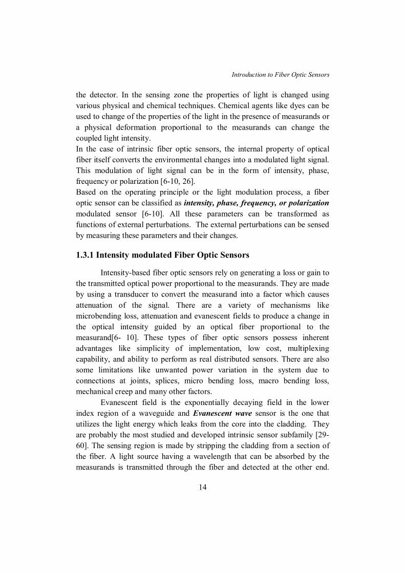
Evanescent field is the exponentially decaying field in the lower

index region of a waveguide and Evanescent wave sensor is the one that

utilizes the light energy which leaks from the core into the cladding. They

are probably the most studied and developed intrinsic sensor subfamily [29-

60]. The sensing region is made by stripping the cladding from a section of

the fiber. A light source having a wavelength that can be absorbed by the

measurands is transmitted through the fiber and detected at the other end.


15

The resulting change in light intensity is a measure of the measurand

concentration [39]. The cladding can also be made sensitive to specific

organic vapors [35] or the cladding of the optical fiber can be replaced along

a small section by a sensitive material [30,31,33]. Any change in the optical

or structural characteristic of the coating material due to the presence of the

measurands generates a change in the effective index of the optical fiber.

Generally fibers have a cladding made of silica, which is difficult to

remove or modify. A remedy is to polish the fiber to eliminate the cladding

[40-42] or using chemical etching where the optical fiber is soaked in

hydrofluoric acid solution [31,43,44]. Plastic cladded fibers (PCS) are an

easy alternative where the cladding can be easily removed either

mechanically or with non hazardous solvents such as acetone [45-48].

Once the cladding is removed or modified the sensing material has to

be fixed onto the fiber core surface. To achieve this analyte is dissolved in a

chemical solution and the fiber is dipped into it several times, known as dip

coating [49,50]. Another method of coating sensitive material is using sol-gel

solutions. Since the sol-gel solution is in liquid phase, the sensing material is

added to it and then the fiber is dipped into the mixture. After drying the

deposition, an optically uniform porous matrix doped with the analyte fixed

onto the fiber is achieved [35,43, 51-57]. Langmuir-Blodgett technique is

another available deposition procedure. The process is based on the

Figure 1.6 Evanescent wave Fiber Optic Sensor System


16

deposition of layers with hydrophobic and hydrophilic behavior, yielding a

homogeneous structure formed by bilayers [58,59].

1.3.2. Wavelength Modulated Fiber Optic Sensors

Wavelength modulated sensors use changes in the wavelength of

light for detection. Fluorescence sensors and fiber grating sensors are

examples of wavelength-modulated sensors. The most widely used

wavelength based sensor is the fiber grating sensor and are generally of two

types namely Fiber Bragg Grating (FBG) and Long Period Fiber Grating

(LPFG) based sensors. In the case of Bragg gratings (FBG) the change is in

the reflection and transmission spectrum, while the variation occurs in the

transmission wavelength in the case of long period fiber a grating (LPFG)

1.3.2.1. Fluorescence sensors

These sensors are based on the spontaneous light emission of a

fluorophore when it is excited with light at a wavelength located in the

absorption spectral region of such fluorophore. The change in the emission

of the dye when it interacts with the measurands is used as the sensing

response. Different schemes have been proposed for fluorescent based fiber

optic sensors and the most popular schemes are fluorescence intensity

sensors, fluorescence lifetime sensors and fluorescence phase-modulation

sensors [61-65].

1.3.2.2. Fiber Gratings

Fiber grating was first reported by Hill et al [66] in 1978 at the

Canadian Communications Research Centre (CRC) and was an outgrowth of

research investigating in nonlinear properties of germania-doped silica fiber.

It is a submicron periodical modulation of the refractive index of the fiber

core coupling light from the forward-propagating mode to a counter

propagating mode of the optical fiber [67-71] and is known as Fiber Bragg

Grating (FBG). In the original experiments an intense Argon-ion laser

(488nm) was launched into a germania-doped fiber and an increase in the

reflected light intensity was noticed with the advancement of time. This light

reflection was due to the formation of periodic refractive index modulation

occurring in the fiber core due to the standing wave pattern formed by the

laser reflected from the fiber end [68]. The technique of grating fabrication

by side illumination was demonstrated by Meltz et al. [72] while a more


17

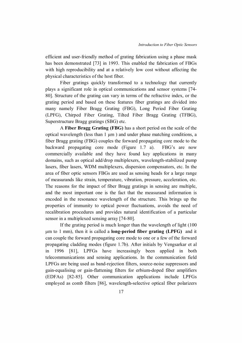
efficient and user-friendly method of grating fabrication using a phase mask

has been demonstrated [73] in 1993. This enabled the fabrication of FBGs

with high reproducibility and at a relatively low cost without affecting the

physical characteristics of the host fiber.

Fiber gratings quickly transformed to a technology that currently

plays a significant role in optical communications and sensor systems [74-

80]. Structure of the grating can vary in terms of the refractive index, or the

grating period and based on these features fiber gratings are divided into

many namely Fiber Bragg Grating (FBG), Long Period Fiber Grating

(LPFG), Chirped Fiber Grating, Tilted Fiber Bragg Grating (TFBG),

Superstructure Bragg gratings (SBG) etc.

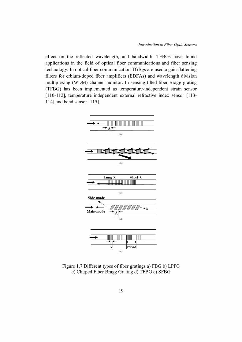
A Fiber Bragg Grating (FBG) has a short period on the scale of the

optical wavelength (less than 1 μm ) and under phase matching conditions, a

fiber Bragg grating (FBG) couples the forward propagating core mode to the

backward propagating core mode (Figure 1.7 a). FBG’s are now

commercially available and they have found key applications in many

domains, such as optical add/drop multiplexers, wavelength-stabilized pump

lasers, fiber lasers, WDM multiplexers, dispersion compensators, etc. In the

area of fiber optic sensors FBGs are used as sensing heads for a large range

of measurands like strain, temperature, vibration, pressure, acceleration, etc.

The reasons for the impact of fiber Bragg gratings in sensing are multiple,

and the most important one is the fact that the measurand information is

encoded in the resonance wavelength of the structure. This brings up the

properties of immunity to optical power fluctuations, avoids the need of

recalibration procedures and provides natural identification of a particular

sensor in a multiplexed sensing array [74-80].

If the grating period is much longer than the wavelength of light (100

μm to 1 mm), then it is called a long-period fiber grating (LPFG) and it

can couple the forward propagating core mode to one or a few of the forward

propagating cladding modes (figure 1.7b). After initials by Vengsarkar et al

in 1996 [81], LPFGs have increasingly been applied in both

telecommunications and sensing applications. In the communication field

LPFGs are being used as band-rejection filters, source-noise suppressors and

gain-equalising or gain-flattening filters for erbium-doped fiber amplifiers

(EDFAs) [82-85]. Other communication applications include LPFGs

employed as comb filters [86], wavelength-selective optical fiber polarizers


18

[87-90], add-drop couplers [91], components in wavelength division

multiplexing (WDM) systems [92-94], or in all-optical switching [95], and

for chromatic dispersion compensation [96]. Though long period fiber

gratings (LPFG) lacks the ability of multiplexing, its high sensitivity to

refractive index gives them an edge over fiber bragg gratings (FBG) in

chemical and biochemical applications.

In a chirped fiber grating (figure 1.7c) the grating period is not

uniform along the length and is achieved by varying the grating period, the

average index, or both along the length of the grating. Chirp in gratings may

take many different forms. The period may vary symmetrically, either

increasing or decreasing in period around a pitch in the middle of a grating

[97-98]. The reflection spectrum of a chirped fiber grating is wider compared

to FBG and each wavelength component is reflected at different positions.

This causes a delay time difference for different reflected wavelengths.

Several techniques to impart chirp was reported namely, exposure to UV

beams of non uniform intensity of the fringe pattern, varying the refractive

index along the length of a uniform period grating, altering the coupling

constant of the grating as a function of position, incorporating a chirp in the

inscribed grating, fabricating gratings in a tapered fiber, applying a non

uniform strain [99-101] etc. All these gratings have special characteristics,

which are like signatures and may be recognized as special features of the

type of grating. Chirped gratings have many applications and have found a

special place in optics as a dispersion-correcting and compensating device.

Ultralong, broad-bandwidth chirped gratings of high quality is used for high-

bit-rate transmission in excess of 40 Gb/sec over 100 km [102]. Some of the

other applications include chirped pulse amplification [103], chirp

compensation of gain-switched semiconductor lasers [104], sensing [68,105],

higher-order fiber dispersion compensation [106], ASE suppression [107],

amplifier gain flattening [108], and band blocking and band-pass filters [109].

In standard FBGs, the grading or variation of the refractive index is

along the length of the fiber (the optical axis) and perpendicular to the

optical axis. In a tilted FBG (TFBG), the variation of the refractive index is

at an angle to the optical axis leading to the occurrence of more complex

mode coupling, as shown in Figure 1.7d. A tilted fiber grating can thus

couple the forward propagating core mode to the backward propagating core

mode and a backward propagating cladding mode and the angle of tilt has an


19

effect on the reflected wavelength, and bandwidth. TFBGs have found

applications in the field of optical fiber communications and fiber sensing

technology. In optical fiber communication TGBgs are used a gain flattening

filters for erbium-doped fiber amplifiers (EDFAs) and wavelength division

multiplexing (WDM) channel monitor. In sensing tilted fiber Bragg grating

(TFBG) has been implemented as temperature-independent strain sensor

[110-112], temperature independent external refractive index sensor [113-

114] and bend sensor [115].

Figure 1.7 Different types of fiber gratings a) FBG b) LPFG c) Chirped Fiber Bragg Grating d) TFBG e) SFBG


20

A sampled fiber Bragg grating (SFBG) or superstructure Bragg

grating (SBG’s) are structures for which parameters vary periodically along

the length of the grating on a scale much larger than the wavelength of light.

They are contra-directional coupling gratings foe which effective refractive

index amplitude and/or phase is modulated through a long periodic structure

(figure 1.7e). The special reflection characteristics of SFBGs make them very

useful and attractive devices for optical communications and fiber sensors

[116-117]. A sampled fiber grating can reflect several wavelength

components with equal wavelength spacing.

1.3.3. Phase Modulated Fiber Optic Sensors

Phase modulated sensors use changes in the phase of light for

detection. The measurands modulate the phase of the light wave passing

through the fiber and this phase modulation is then detected

interferometrically [6-10,118-127]. Mach-Zehnder and Michelson [118-119],

Fabry-Perot [120-126], Sagnac [127] and grating interferometers [123, 126]

are the most commonly used intereferometers. Fiber Fabry-Perot

interferometric sensor (FFPI) is the commonly used interferometer based

sensor and is classified into two categories namely Intrinsic Fabry-Perot

interferometer (IFPI) sensor [121-122] and Extrinsic Fabry-Perot

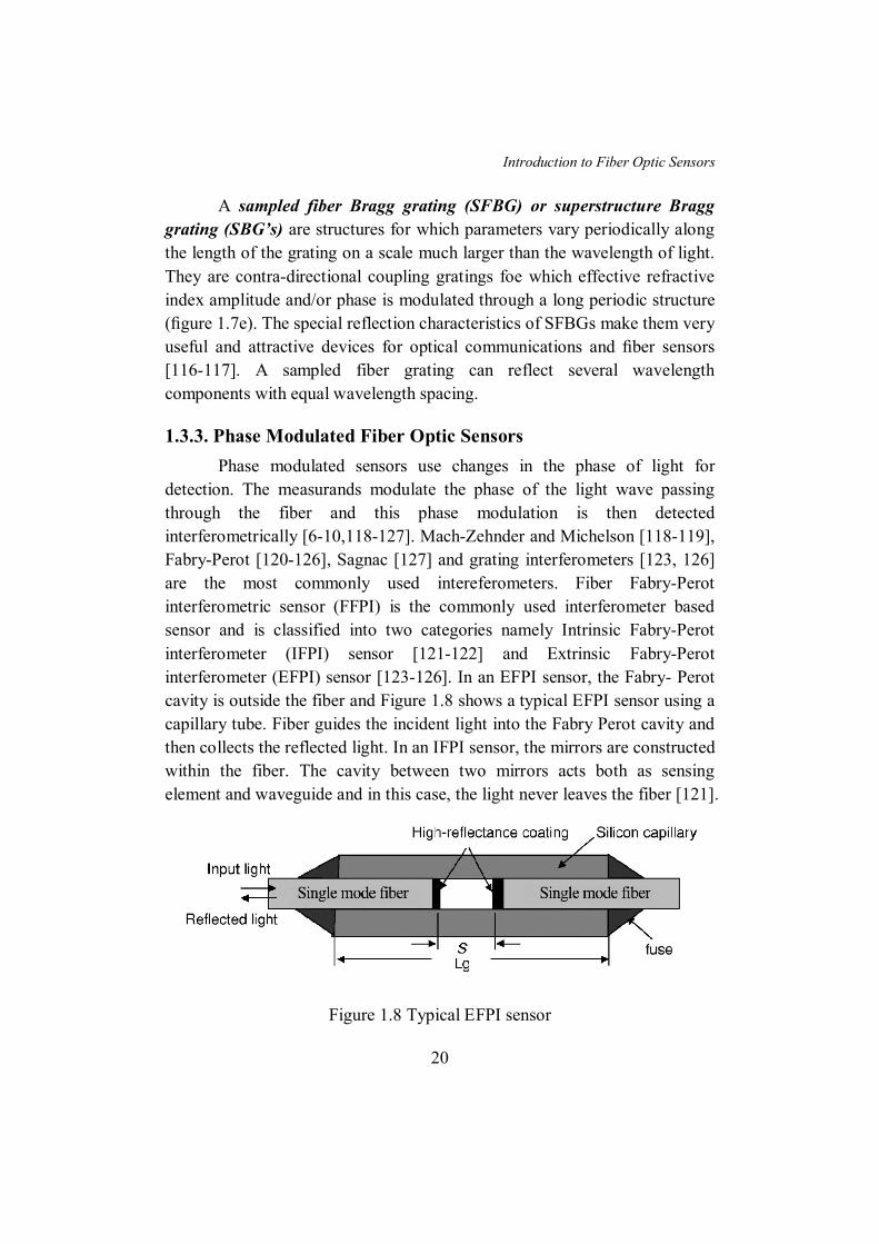
interferometer (EFPI) sensor [123-126]. In an EFPI sensor, the Fabry- Perot

cavity is outside the fiber and Figure 1.8 shows a typical EFPI sensor using a

capillary tube. Fiber guides the incident light into the Fabry Perot cavity and

then collects the reflected light. In an IFPI sensor, the mirrors are constructed

within the fiber. The cavity between two mirrors acts both as sensing

element and waveguide and in this case, the light never leaves the fiber [121].

Figure 1.8 Typical EFPI sensor


21

1.3.4. Polarization Modulated Fiber Optic Sensors

The direction of the electric field portion of the light field is defined

as its polarization state and the fiber optic sensors based on detection of

change in induced phase difference between different polarization directions

are termed as Polarization Modulated Fiber Optic Sensors. The refractive

index of a fiber varies when it undergoes stress or strain and the induced

refractive index change occurs in the direction of applied stress or strain.

Thus an induced phase difference is created between different polarization

directions and this phenomenon is called photoelastic effect. Therefore, by

detecting the change in the output polarization state, the external perturbation

can be sensed [9].

1.4 Fiber Optic Sensors in Quality evaluation

Quality is defined as the standard of something as measured against

other things of a similar kind or in other words the degree of excellence of

something. The definition of quality depends on the role of the people

defining it and on the material on which it is defined. Some people view

quality as “performance to standards” while some view it as “meeting the

customer’s needs” or “satisfying the customer.” The difficulty in defining

quality exists regardless of product, and this is true for both manufacturing

and quality control organizations.

The evaluation of quality of a product is thus important in both the

production side and consumer side. It can be either done manually or

automatically and both methods have its own merits and demerits.

Traditionally quality evaluation is done manually and it requires skilled

operators and the process is time consuming. Moreover, the chances for

human error are more in this process. On contrary automatic quality

evaluation is fast, cost effective and accurate.

Sensors are the vital elements of such automatic quality evaluation

systems where appropriate sensors with high sensitivity and resolution are a

necessity and sensors based on various technologies have carved their niches

in their areas. One of the major application area of fiber optic sensors is in

monitoring the physical health of structures like buildings, bridges, tunnels,

dams and heritage structures in real time. Concrete monitoring during setting,

crack (length, propagation speed) monitoring, pre stressing monitoring,


22

spatial displacement measurement, neutral axis evolution, long-term

deformation (creep and shrinkage) monitoring, concrete-steel interaction,

and post-seismic damage evaluation are some of the civil engineering

parameters measured using fiber optic sensors [128-131]. Twenty-six FBG

strain sensors have been reported to be monitoring the Horsetail Falls Bridge

in Oregom successfully for 2 years [132]. The bridge was originally built in

1914 and in 1998 it was strengthened by placing composite wraps over the

concrete beams. Bragg grating strain sensors have been employed for

monitoring the prestressing tendons of the Beddington Trail Bridge, Canada

[133] and Tsing Ma Bridge in China [134]. Gebremichael et al. in 2005 have

reported the use of 40 FBG sensors to remotely monitor the real-time strain

on Europe’s first all-fiber reinforced composite bridge, The West Mill

Bridge [135]. In situ monitoring of strain data from the bridge and to analyze

this data for assessment of its structural integrity, maintenance scheduling

and validation of design codes are the main objective behind this study.

Quality measurement of reinforced concrete beams instrumented with FBG

sensors have been reported in literatures [136-140]. Bragg grating sensors

have been used successfully to monitor the strain in concrete piles [141-144]

and are essential since piles carry the weight of the foundation and transmit

the load of the structure to the subsoil. Another area where quality

monitoring is essential is the cement curing process which is affected by the

water to cement ratio, the curing temperature, humidity and type of cement

used. FBG strain sensors have been used to study early-age cement paste

shrinkage [145] and the shrinkage and temperature change behavior of

reactive powder concrete (RPC) in the early age was studied by Wong et al.

[146]. M. Rajesh et. al [147] did studies on the setting characteristics of

various grades of cement while plastic optical fibers were successfully used

for cement setting studies by Andrea et.al [148].

Adulteration in food is a major area of concern and a fiber optic

sensor for determining quality of coconut oil was reported by Sheeba et al

[149]. An evanescent type fiber optic sensor using a side polished plastic

clad silica fiber was used in their work. Altering the quality of fuels is

another major problem faced world wide and fiber optic sensors were

successfully developed to test the purity of petrol and diesel. [150-153].

While Mishra et.al [153] developed long period based sensor for identifying

kerosene adulteration in petrol, a similar technique was utilized by Falate


23

et.al [151] for Biodiesel Quality Control. Fiber optic sensors supervised by

artificial neural networks were demonstrated as integrate systems for smart

sensing in fuel industry by Possetti et.al [152].

Another important area is contamination of water where authors have

reported works on pH detection using optical methods [154-160]. Ganesh

et.al [154] used a membrane made of cellulose acetate for reagent

immobilization and congo red (pKa 3.7) and neutral red (pKa 7.2) as pH

indicators while a sol–gel derived film doped with a pH indicator

bromocresol purple (BCP) was reported by Burke et.al [160]. Long Period

Fiber Gratings (LPFG) based in-fiber Mach–Zehnder interferometer for

salinity measurement in a water solution was reported by Possetti et. al [161]

and Samer et.al [162]. Ethanol concentration detection in alcohol beverages

is another area where adulteration is common and an optical-fiber sensor

using the fluorescence induced by a laser-diode-pumped Tm3+:YAG for

determining water concentrations in ethanol–water and methanol–water

mixtures was reported by Yokota et.al [163]. A fiber-optic sensor with a

chitosan/poly(vinyl alcohol) blended membrane as the cladding was

fabricated to determine ethanol in alcoholic beverages by Kurauchi et. al

[164]

Quality of air depends on the concentration of many parameters and

their measurement in various environments is a necessity. Humidity is one

such parameter and its precise measurement is inevitable in various industrial

and domestic environments and various authors have presented fiber optic

sensors for humidity detection [165-171]. Long Period Fiber Grating based

humidity sensor with PVA coating was reported by Venugopalan et. al [165-

167] while Liwei Wang et. al [166] and Arregui et. al [169] used hydro gel

as the sensitive material. An Optical fiber based humidity sensor using

cobalt-polyaniline as sensitive cladding material was reported by Anu

Vijayan et. al [171]. Measurement of ammonia concentration is important in

industrial environments and Wenqing Cao et. al. [172] have developed an

optical fiber based sensor system using sol-gel immobilized bromocresol

purple (BCP). An ammonia sensor using a pH Indicator dye p-nitrophenol

was reported by Arnold et.al. [173]. Fiber optic gas sensors were reported for

the detection of Oxygen [174], carbon dioxide [175-177], hydrogen [178]

and nitrogen dioxide [179-181]. Mahesh et.al.[175] have developed a carbon

dioxide sensor for fermentation monitoring while Shelly et.al.[181] reported


24

a sensor with nanoporous structure for the selective detection of NO2 in air

samples.

Conclusions

In this chapter we discussed the basics of optical fiber and

fiber optic sensor technology. The theory of light guiding in an optical fiber

was explained along with various types of fiber sensor configurations, their

advantages and disadvantages. Fiber sensors are being investigated for the

past forty years and some of the findings related to their applications in

quality evaluation of civil structures, liquids and air are discussed in this

chapter.

References

1. V. P. N. Nampoori, “Dream Merchants-The Evolution of Fiber Optics”, http://photonics.cusat.edu/Article1.html

2. K. C. Kao and G. A. Hockham, “Dielectric-fiber surface waveguides for optical frequencies”, Proc. IEE 113, 1151-1158 (1966)

3. Charles K. Kao, “Nobel Lecture: Sand from centuries past: Send future voices fast”, Rev. Mod. Phys. 82, 2299-2303 (2010)

4. K. Saito, M. Yamaguchi, H. Kakiuchida, A. J. Ikushima, K. Ohsono and Y. Kurosawa, “Limit of the Rayleigh scattering loss in silica fiber”, Appl. Phys. Lett. 83, 5175-5177 (2003)

5. F. Poletti, N. V. Wheeler,M. N. Petrovich,N. Baddela, E. Numkam Fokoua, J. R. Hayes, D. R. Gray, Z. Li, R. Slavík and D. J. Richardson, “Towards high-capacity fiber-optic communications at the speed of light in vacuum”, Nature Photonics 7, 279–284 (2013)

6. B Culshaw and J Dakin, Optical Fiber Sensors: Systems and Applications, (Artech House, Boston, 1989)

7. D A Krohn, Fiber Optic Sensors: Fundamental and Applications, (Instrument Society of America, Research Triangle Park, North Carolina, 1988).

8. E Udd, Fiber Optic Sensors: An Introduction for Engineers and Scientists, (Wiley, New York, 1991).

9. Francis To So Yu and Shizhuo Yin, Fiber Optic Sensors, (Marcel Dekker, Inc. New York, 2002).

10. B.D.Gupta, Gupta and Banshi Das, Fiber Optic Sensors: Principles and Applications (New India Publishing, New Delhi,2006)

11. Daru Chen, Weisheng Liu, Meng Jiang, and Sailing He, “High-Resolution Strain/Temperature Sensing System Based on a High-Finesse Fiber Cavity and Time-Domain Wavelength Demodulation”, J. Lightwave Technol. 27, 2477-2481 (2009)


25

12. N. Lagakos, J. A. Bucaro, and J. Jarzynski, "Temperature-Induced Optical Phase Shifts in Fibers," Appl. Opt. 20, 2305-2308 (1981).

13. H. Y. Fu, H. Y. Tam, L. Y. Shao, X. Dong, P. K. A. Wai, C. Lu, and S. K. Khijwania, "Pressure sensor realized with polarization-maintaining photonic crystal fiber-based Sagnac interferometer," Appl. Opt. 47, 2835-2839 (2008).

14. A. B. Tveten, A. Dandridge, C. M. Davis, and T. G. Giallorenzi, "Fiber Optic Accelerometer" Electron. Lett.16, 854-856 (1980).

15. V. Vali, R.W. Shorthill, “Fiber ring interferometer”, Appl. Opt. 15, 1099–1100 (1976).

16. Sven Kuehn, Fin Bomholt and Niels Kuste, “Miniature Electro-Optical Probe for Magnitude, Phase and Time-Domain Measurements of Radio-Frequency Magnetic Fields”, (Asia-Pacific International Symposium on Electromagnetic Compatibility, Institute of Electrical and Electronics Engineers, New York, 2010)

17. A.H. Rose, Z.B. Ren, G.W. Day, “Twisting and annealing optical fiber for current sensors”, J. Lightwave Technol. 14, 2492–2498 (1996).

18. G.D. Peng, P.L. Chu, “Optical fiber hydrophone systems”, in: F.T.S. Yu, S. Yin (Eds.), Fiber Optic Sensors (Dekker, New York, 2002).

19. Colette McDonagh, Conor S. Burke and Brian D. MacCraith, “Optical Chemical Sensors”, Chem. Rev. 108, 400-422 (2008).

20. Otto S. Wolfbeis, “Fiber-Optic Chemical Sensors and Biosensors”, Anal. Chem.78, 3859-3874 (2006).

21. Otto S. Wolfbeis, “Fiber-Optic Chemical Sensors and Biosensors”, Anal. Chem. 80, 4269–4283 (2008).

22. M.D. Marazuela, M.C. Moreno-Bondi, “Fiber-optic biosensors—an overview”, Anal. Bioanal. Chem. 372, 664–682 (2002).

23. K Okamoto, Fundamentals of optical waveguides, (Academic Press. San Diego 2000).

24. G Keiser, Optical fiber communications. (3rd ed.). (McGraw-Hill, Singapore, 2000)

25. D Gloge, “Weakly guiding fibers”, Appl.Opt. 10, 2252-2258 (1971).

26. Culshaw B,Stewart G, Dong F, Tandy C, Moodie D, “Fiber optic techniques for remote spectroscopic methane detection-from concept to system realization”. Sensor. Actuat. B-Chem. 51, 25-37 (1998).

27. Stewart G, Tandy C, Moodie, D, Morante, M.A, Dong F, “Design of a fiber optic multi-point sensor for gas detection”, Sensor. Actuat. B-Chem. 51, 227-232 (1998).

28. Ho H.L, Jin W, Yu H.B, Chan K.C, Chan C.C, Demokan M.S, “Experimental demonstration of a Fiber-Optic Gas Sensor Network Addressed by FMCW”, IEEE Photon. Tech. Lett. 12, 1546-1548 (2000).

29. Tracey, P. M., “Intrinsic Fiber-Optic Sensors”, IEEE Trans. Ind. Appl. 27, 96-98 (1991)

30. Khijwania S.K, Gupta B.D, “Fiber optic evanescent field absorption sensor with high sensitivity and linear dynamic range”, Opt. Commun.152, 259-262 (1998)

31. Khalil S, Bansal L, El-Sherif M, “Intrinsic fiber optic chemical sensor for the detection of dimethyl methylphosphonate”, Opt. Eng. 43, 2683-2688 (2004).


26

32. Dickinson T.A, Michael K.L, Kauer J.S, Walt D.R, “Convergent, Self-Encoded Bead Sensor Arrays in the design of an Artificial Nose”, Anal. Chem. 71, 2192-2198 (1999).

33. Yuan J, El-Sherif A, “Fiber-Optic Chemical Sensor Using Polyaniline as Modified Cladding Material”, IEEE Sensor. J. 3, 5-12 (2003).

34. Messica A, Greenstein A, Katzir A, “Theory of fiber-optic, evanescent-wave spectroscopy and sensors”, Appl. Opt. 35, 2274-2284 (1996).

35. Schwotzer G, Latka I, Lehmann H.,Willsch R, “Optical sensing of hydrocarbons in air or in water using UV absorption in the evanescent field of fibers”, Sensor. Actuat. B-Chem. 38-39, 150-153 (1997).

36. Shadaram M, Espada L, Garcoa F, “Modeling and performance evaluation of ferrocene-based polymer clad tapered optical fiber gas sensors”, Opt. Eng. 37, 1124-1129 (1998)

37. Barmenkov Y.O, “Time-domain fiber laser hydrogen sensor”, Opt. Lett. 29, 2461-2463 (2004).

38. Lacroix S, Bourbonnais R, Gonthier F, Bures J, “Tapered monomode optical fibers: understanding large power transfer” Appl. Opt. 25, 4421-4425 (1986).

39. Willer U, Scheel D, Kostjucenko I, Bohling C, Schade W, Faber E, “Fiber-optic evanescent-field laser sensor for in-situ gas diagnostics”, Spectrochim. Acta A 58, 2427-2432 (2002).

40. Senosiain J, Díaz I, Gastón A, Sevilla J, “High Sensitivity Temperature Sensor Based on Side-Polished Optical Fiber”, IEEE Trans. Instrum. Meas. 50, 1656-1660 (2001).

41. Gastón A, Pérez F, Sevilla J, “Optical fiber relative-humidity sensor with polyvinyl alcohol film”, Appl. Opt. 43, 4127-4132 (2004)

42. Gastón A, Lozano I, Pérez F, Auza F, Sevilla J, “Evanescent Wave Optical-Fiber Sensing (Temperature, Relative Humidity and pH Sensors)”, IEEE Sensor. J. 3, 806-811 (2003).

43. Sumdia S, Okazaki S, Asakura S, Nakagawa H, Murayama H, Hasegawa T, “Distributed hydrogen determination with fiber-optic sensor”, Sensor. Actuat. B-Chem. 108, 508-514 (2005).

44. Segawa H, Ohnishi E, Arai Y, Yoshida K, “Sensitivity of fiber-optic carbon dioxide sensors utilizing indicator dye”, Sensor. Actuat. B-Chem. 94, 276-281 (2003).

45. Cherif K, Mrazek J, Hleli S, Matejec, V, Abdelghani, A Chomat M, Jaffrezic-Renault N, Kasik I, “Detection of aromatic hydrocarbons in air and water by using xerogel layers coated on PCS fibers excited by an inclined collimated beam”, Sensor. Actuat. B-Chem. 95, 97-106 (2003).

46. Malis C, Landl M, Simon P, MacCraith B.D, “Fiber optic ammonia sensing employing novel near infrared dyes” Sensor. Actuat. B-Chem. 51, 359-367 (1998).

47. Potyrailo R.A, Hieftje G.M, “Oxygen detection by fluorescence quenching of tetraphenylporphyrin immobilized in the original cladding of an optical fiber”, Anal. Chim. Acta. 370, 1-8 (1998).

48. Okazaki S, Nakagawa H, Asakura S, Tomiuchi Y,Tsuji N, Murayama H, Washiya M, “Sensing Characteristics of an optical fiber sensor for hydrogen leak” Sensor. Actuat. B-Chem. 93, 142-147 (2003).


27

49. Ho H.L, Jin W, Yu H.B, Chan K.C, Chan C.C, Demokan M.S, “Experimental demonstration of a Fiber-Optic Gas Sensor Network Addressed by FMCW”, IEEE Photon. Tech. Lett. 12, 1546-1548 (2000).

50. Scorsone E, Christie S, Persaud K.C, Simon P, Kvasnik F, “Fiber-optic evanescent sensing of gaseous ammonia with two forms of a new near-infrared dye in comparison to phenol red”, Sensor. Actuat. B-Chem. 90, 37-45 (2003).

51. Sekimoto S, Nakagawa H, Okazaki S, Fukuda K, Asakura S, Shigemori T, Takahashi S, “A Fiber-optic evanescent-wave hydrogen gas sensor using palladium-supported tungsten oxide”, Sensor. Actuat. B-Chem. 66, 142-145 (2000).

52. Jorge P.A.S, Caldas P, Rosa C.C, Oliva A.G, Santos J.L, “Optical fiber probes for fluorescente based oxygen sensing”, Sensor. Actuat. B-Chem. 130, 290-299 (2004).

53. Grant S.A, Satcher J.H. Jr, Bettencourt K, “Development of sol-gel-based fiber nitrogen dioxide gas sensors”, Sensor. Actuat. B-Chem. 69, 132-137 (2000).

54. Abdelghani A, Chovelon J.M, Jaffrezic-Renault N, Lacroix M, Gagnaire H, Veillas C, Berkova B, Chomat M, Matejec V, “Optical fiber sensor coated with porous silica layers for gas and chemical vapour detection”, Sensor. Actuat. B-Chem. 44, 495-498 (1997).

55. Abdelmalek F, Chovelon J.M, Lacroix M, Jaffrezic-Renault N, Matajec V, “Optical fiber sensors sensitized by phenyl-modified porous silica prepared by sol-gel”, Sensor. Actuat. B-Chem. 56, 234-242 (1999)

56. Bariain C, Matias I.R, Romeo I, Garrido J, Laguna M, “Detection of volatile organic compund vapors by using a vapochromic material on a tapered optical fiber”, Appl. Phys. Lett. 77, 2274-2276 (2000).

57. Bariain C, Matias I.R, Romeo I, Garrido J, Laguna M, “Behavioral experimental studies of a novel vapochromic material towards development of optical fiber organic compounds sensor”, Sensor. Actuat. B-Chem. 76, 25-31 (2001).

58. Hu W, Liu Y, Xu Y, Liu S, Zhou S, Zeng P, Zhu D.B, “The gas sensitivity of Langmuir-Blodgett films of a new asymmetrically substituted phthalocyanine”, Sensor. Actuat. B-Chem. 56, 228-233 (1999).

59. Bariain C, Matias I.R, Fernandez-Valdivielso C, Arregui F.J, Rodríguez-Méndez M.L, De Saja J.A, “Optical fiber sensor based on lutetium bisphthalocyanine for the detection of gases using standard telecommunication wavelengths”, Sensor. Actuat. B-Chem. 93, 153-158 (2003).

60. Gutierrez N, Rodríguez-Méndez M.L, De Saja J.A, “Array of sensors based on lanthanide bisphthalocyanine Langmuir-Blodgett films for the detection of olive oil aroma”, Sensor. Actuat. B-Chem. 77, 437-442 (2001).

61. Mitsubayashi K, Minamide T, Otsuka K, Kudo H, Saito H, “Optical bio-sniffer for methyl mercaptan in halitosis”, Anal. Chim. Acta, 573, 75-80.( 2006).

62. Wolfbeis O.S, Kovacs B, Goswami K, Klainer S.M, “Fiber-Optic Fluorescence Carbon Dioxide Sensor for Environmental Monitoring”, Mikrochim. Acta. 129, 181-188 (1998).

63. Kim Y.C, Peng W, Banerji S, Booksh K.S, “Tapered fiber optic surface plasmon resonance sensor for analyses of vapor and liquid phases”, Opt. Lett. 30, 2218-2220 (2005)


28

64. O’Neal P.D, Meledeo A, Davis J.R, Ibey B.L, Gant V.A, Pishko M.V, Cote G.L, “Oxygen Sensor Based on the Fluorescence Quenching of a Ruthenium Complex Immobilized in a Biocompatible Poly(Ethylene Glycol) Hydrogel”, IEEE Sensor. J. 4, 728-734 (2004).

65. Grattan K.T.V, Zhang Z.Y, “Fiber Optic Fluorescence Thermometry”, (Chapman & Hall: London, 1995).

66. K.O. Hill, Y. Fujii, D.C. Johnson, B.S. Kawasaki “Photosensitivity in optical fiber waveguides: application to reflection filter fabrication”, Appl. Phys. Lett. 32 647–649 (1978).

67. Raman Kashyap, “Fiber Bragg Gratings”, (Academic Press, San Diego, USA 1999).

68. K.O. Hill and Gerald Meltz, “Fiber Bragg Grating Technology Fundamentals and Overview”, J. Lightwave Technol. 15 ,1263-1276 (1997)

69. K.O. Hill, “Photosensitivity in Optical Fiber Waveguides: From Discovery to Commercialization”, IEEE J. Sel. Top. Quantum Electron. 6, 1186-1189 (2000)

70. Andreas Othonos, “Fiber Bragg gratings”, Rev. Sci. Instrum. 68 ,4309-4341 (1997)

71. Turan Erdogan, “Fiber Grating Spectra”, J. Lightwave Technol. 15, 1277-1294 (1997)

72. G. Meltz, W.W. Morey, W.H. Glenn, Formation of Bragg gratings in optical fibers by a transverse holographic method”, Opt. Lett. 14, 823–825 (1989).

73. K. O. Hill, B Malo, F. Bilodeau, D. C. Johnson, and J. Albert, “Bragg gratings fabricated in monomode photosensitive optical fiber by UV exposure through a phase mask”, Appl. Phys. Lett. 62, 1035-1037(1993).

74. O. Frazao,L. A. Ferreira, F. M. Araujo, J. L. Santos, “Applications of Fiber Optic Grating Technology to Multi-Parameter Measurement”, Fiber Integr. Opt. 24, 227–244 (2005).

75. Giles, C. R. “Lightwave applications of fiber Bragg gratings”, J. Lightwave Technol. 15, 1391-1395 (1997)

76. Yun-Jiang Rao, “In-fiber Bragg grating sensors”, Meas. Sci. Technol. 8 , 355–375 (1997)

77. A. D. Kersey, M. A. Davis, H. J. Patrick, M. LeBlanc, K. P. Koo, C. G. Askins, M. A. Putnam, and E. J. Friebele, "Fiber grating sensors," J. Lightwave Technol. 15, 1442-1462 (1997).

78. Alan D. Kersey, Michael A. Davis, Heather J. Patrick, Michel LeBlanc, K. P. Koo, C. G. Askins, M. A. Putnam, and E. Joseph Friebele, “Fiber Grating Sensors”, J. Lightwave Technol. 15, 1442-1463 (1997)

79. Y.J. Rao, “Recent progress in applications of in-fiber Bragg grating sensors”, Opt. Lasers Eng. 31, 297-324 (1999)

80. Byoungho Lee, “Review of the present status of optical fiber sensors”, Opt. Fiber Technol. 9, 57-79 (2003)

81. Vengsarkar A.N., Lemaire P.J., Judkins J.B., Bhatia V., Erdogan T. and Sipe J.E, “Long-period fiber gratings as band-rejection filters”. J. Lightwave Technol. 14,58-65 (1996).

82. James S.W. and Tatam R.P., “Optical fiber long-period grating sensors: characteristics and applications”, Meas. Sci. Technol. 14, R49-R61 (2003).


29

83. Vengsarkar A.N., Pedrazzani J.R., Judkins J.B. and Lemaire P.J., “Longperiod fiber-grating-based gain equalizers”, Opt. Lett. 21,336-338 (1996).

84. Wysocki P.F., Judkins J.B., Espindola R.P., Andrejco M. and Vengsarkar A.M., “Broad-band erbium-doped fiber amplifier flattened beyond 40 nm using long-period grating filter”, IEEE Photonics Technol. Lett. 9, 1343-1345 (1997).

85. Frazão O., Rego G., Lima M., Teixeira A., Araújo F.M., André P., Da Rocha J.F.and Salgado H.M., “EDFA gain flattening using long-period fibergratings based on the electric arc technique”, (Proceedings of the London Communications Symposium-LCS2001, 2001)

86. Gu X.J., “Wavelength-division multiplexing isolation fiber filter and light source using cascaded long-period fiber gratings”, Opt. Lett. 23, 509-510 (1998).

87. Ortega B., Dong L., Liu W.F., De Sandro J.P., Reekie L., Tsypina S.I., Bagratashvili V.N. and Laming R.I., “High-performance optical fiber polarizers based on long-period gratings in birefringent optical fibers”, IEEE Photonics Technol. Lett. 9,1370-1372 (1997).

88. Kurkov A.S., Douay M., Duhem O., Leleu B., Henninot J.F., Bayon J.F. and Rivoallan L., “Long-period fiber grating as a wavelength selective polarisation element”, Electron. Lett. 33, 616-617 (1997).

89. Kurkov A.S., Vasil’ev S.A., Korolev I.G., Medvedkov O.I. and Dianov E.M., “Fiber laser with an intracavity polariser based on a long-period fiber grating”, Quantum Electron. 31, 421-423 (2001).

90. Zhang L., Liu Y., Everall L., Williams J.A.R. and Bennion I., “Design and realization of long-period grating devices in conventional and high birefringence fibers and their novel applications as fiber-optic load sensors”, IEEE J. Sel. Top. Quantum Electron. 5, 1373-1378 (1999).

91. Chiang K.S., Liu Y., Ng M.N. and Li S., “Coupling between two parallel long-period fiber gratings”, Electron. Lett. 36, 1408-1409 (2000).

92. Laffont G. and Ferdinand P., “Fiber Bragg grating-induced coupling to cladding modes for refractive index measurements”, Proc. SPIE 4185, 326-329 (2000).

93. Lam P.K., Stevenson A.J. and Love J.D., “Bandpass spectra of evanescent couplers with long period gratings”, Electron. Lett. 36, 967-969 (2000).

94. Zhu Y., Lu C., Lacquet B.M., Swart P.L. and Spammer S.J., “Wavelength tunable add/drop multiplexer for dense wavelength division multiplexing using long-period gratings and fiber stretchers:, Opt. Commun. 208, 337-344 (2002).

95. Eggleton B.J., Slusher R.E., Judkins J.B., Stark J.B. and Vengsarkar A.M., “All-optical switching in long-period fiber gratings”, Opt. Lett. 22, 883-885 (1997).

96. Das M. and Thyagarajan K. , “Dispersion compensation in transmission using uniform long period fiber gratings”, Opt. Commun. 190, 159-163 (2001).

97. Byron K. C., Sugden K, Bircheno T. and Bennion I., "Fabrication of chirped Bragg gratings in photosensitive fiber," Electron. Lett. 29, 1659 (1993).

98. Parries M. C., Sugden K., Reid D. C. J., Bennion L, Molony A. and Goodwin M. J., "Very broad reflection bandwidth (44 nm) chirped fiber gratings and narrow-bandpass filters produced by the use of an amplitude mask," Electron. Lett. 30, 891-892 (1994).

99. Stephens T, Krug P. A., Brodzeli Z., Doshi G., Ouellette R and Poladin L., "257 km transmission at 10 Gb/s in non dispersion shifted fiber using an unchirped


30

fiber Bragg grating dispersion compensator," Electron. Lett. 32, 1559-1561 (1996).

100. Kashyap R., McKee P. R, Campbell R. J. and Williams D. L., "A novel method of writing photo-induced chirped Bragg gratings in optical fibers," Electron. Lett. 30, 996-997 (1994).

101. Putnam M. A., Williams G. M. and Friebele E. J., " 'Fabrication of tapered, strain-gradient chirped fiber Bragg gratings," Electron. Lett. 31, 309-310 (1995).

102. Loh W. H., Laming R. I., Robinson N., Cavaciuti A., Vaninetti, Anderson C. J., Zervas M. N. and Cole M. J., "Dispersion compensation over distances in excess of 500 km for 10 Gb/s systems using chirped fiber gratings," IEEE Photon. Technol. Lett. 8, 944 (1996).

103. Boskovic A., Guy M. J., Chernikov S. V., Taylor J. R. and Kashyap R., "All fiber diode pumped, femtosecond chirped pulse amplification system," Electron.Lett. 31, 877-879 (1995).

104. Gunning P., Kashyap R., Siddiqui A. S. and Smith K., "Picosecond pulse generation of <5 ps from gain-switched DFB semiconductor laser diode using linearly step-chirped fiber grating," Electron. Lett. 31, 1066-1067 (1995).

105. M.G. Xu, L. Dong, L. Reekie, J.A. Tucknott and J.L. Cruz, “Temperature-independent strain sensor using a chirped Bragg grating in a tapered optical fiber”, Electron.Lett. 31, 823 – 825 (1995).

106. Williams J. A. R., Bennion I. and Doran N. J. "The design of in-fiber Bragg grating systems for cubic and quadratic dispersion compensation," Opt. Commun.,116, 62-66 (1995).

107. Fairies M. C., Ragdale G. M. and Reid D. C. J., "Broadband chirped fiber Bragg grating filters for pump rejection and recycling in erbium doped fiber amplifiers," Electron. Lett. 28, 487-489 (1992).

108. Kashyap R., Wyatt R. and McKee P. F, "Wavelength flattened saturated erbium amplifier using multiple side-tap Bragg gratings," Electron. Lett. 29, 1025-1027 (1993).

109. Zhang I., Sugden K, Williams J. A. R. and Bennion I., "Postfabrication exposure of gap-type bandpass filters in broadly chirped fiber gratings," Opt. Lett. 20, 1927-1929 (1995).

110. Kang S C, Kim S Y, Lee S B, Kwon S W, Choi S S and Lee B, “Temperature-independent strain sensor system using a tilted fiber Bragg grating demodulator”, IEEE Photon. Technol. Lett. 10, 1461–1463 (1998).

111. Chen C, Xiong L, Jafari A and Albert J, “Differential sensitivity characteristics of tilted fiber Bragg grating sensors”, Proc. SPIE. 6004, 6004–6013 (2005).

112. Chen X, Zhou K, Zhang L and Bennion I, “ In-fiber twist sensor based on a fiber Bragg grating with 81 degrees tilted structure”, IEEE Photon. Technol. Lett. 18, 2596–2604 (2006).

113. Laffont G and Ferdinand P, “Tilted short-period fiber-Bragg-grating-induced coupling to cladding modes for accurate refractometer”, Meas. Sci. Technol. 12, 765–770 (2001)

114. Chan C F, Chen C, Jafari A, Laronche A, Thomson D J and Albert J, “Optical fiber refractometer using narrowband cladding mode resonance shifts”, Appl. Opt. 46, 1142–1149 (2007)


31

115. Baek S, Jeong Y and Lee B, “Characteristics of short-period blazed fiber Bragg gratings for use as macro-bending sensors”, Appl. Opt. 41, 631–636 (2002)

116. Frazao O, Romero R, Rego G, Marques P V S, Salgado H M and Santos J L, “Sampled fiber Bragg grating sensors for simultaneous strain and temperature measurement”, Electron. Lett. 38 693–695 (2002)

117. Neil J. Baker, Ho W. Lee, Ian C. M. Littler, C. Martijn de Sterke, Benjamin J. Eggleton, Duk-Yong Choi, Steve Madden and Barry Luther-Davies, “Sampled Bragg gratings in chalcogenide (As2S3) rib-waveguides”, Opt. Express 14, 9451-9459 (2006)

118. Zhaobing Tian, Scott S-H. Yam and Hans-Peter Loock, “Single-Mode Fiber Refractive Index Sensor Based on Core-Offset Attenuators”, IEEE Photon. Tech. Lett. 20, 1387-1389 (2008).

119. T. Allsop, R. Reeves, D. J. Webb, and I. Bennion, “A high sensitivity refractometer based upon a long period grating Mach–Zehnder interferometer”, Rev. Sci. Instrum. 73, 1702-1705 (2002)

120. Yuan-Tai Tseng, Yun-Ju Chuang, Yi-ChienWu, Chung-Shi Yang, Mu-ChunWang and Fan-Gang Tseng, “A gold-nanoparticle-enhanced immune sensor based on fiber optic interferometry”, Nanotechnology 19, 345501(1-9) (2008)

121. Christopher J Tuck, Richard Hague and Crispin Doyle, “Low cost optical fiber based Fabry–Perot strain sensor production”, Meas. Sci. Technol. 17 ,2206–2212 (2006)

122. Tao Wei, Yukun Han, Yanjun Li, Hai-Lung Tsai, and Hai Xiao, “Temperature-insensitive miniaturized fiber inline Fabry-Perot interferometer for highly sensitive refractive index measurement”, Opt. Express 16, 5764-5769 (2008).

123. Yun-Jiang Rao, “Recent progress in fiber-optic extrinsic Fabry–Perot interferometric sensors”, Opt. Fiber Technol. 12, 227–237 (2006

124. Vikram Bhatia, Kent A Murphy, Richard 0 Claus, Mark E Jones, Jennifer L Grace, Tuan A Tran and Jonathan A Greene, “Multiple strain state measurements using conventional and absolute optical fiber-based extrinsic Fabry-Perot interferometric strain sensors”, Smart Mater. Struct. 4, 240-245 (1995)

125. Vikram Bhatia, Kent A Murphy, Richard 0 Claus, Mark E Jones, Jennifer L Grace, Tuan A Tran and Jonathan A Greene, “Optical fiber based absolute extrinsic Fabry–P´erot interferometric sensing system”, Meas. Sci. Technol. 7 ,58–61 (1996).

126. Yun-Jiang Rao, Zeng-Ling Ran, Xian Liao, and Hong-You Deng, “Hybrid LPFG/MEFPI sensor for simultaneous measurement of high-temperature and strain”, Opt. Express 15, 14936-14941(2007).

127. A. N. Starodumov, L. A. Zenteno, D. Monzon and E. De La Rosa, “Fiber Sagnac interferometer temperature sensor”, Appl. Phys. Lett. 70 ,19-21 (1997).

128. F. Ansari, “State-of-the-art in the applications of fiber-optic sensors to cementitious composites”, Cem. Concr. Compos. 19, 3–19 (1997).

129. R.C. Tennyson, A.A. Mufti, S. Rizkalla, G. Tadros, B. Benmokrane, “Structural health monitoring of innovative bridges in Canada with fiber optic sensors”, Smart Mater. Struct. 10, 560–573 (2001).

130. Y.B. Lin, C.L. Pan, Y.H. Kuo, K.C. Chang, “Online monitoring of highway bridge construction using fiber Bragg grating sensors”, Smart Mater. Struct. 14, 1075–1082 (2005).


32

131. Y.B. Lin, J.S. Lai, K.C. Chang, L.S. Li, “Flood scour monitoring system using fiber Bragg grating sensors”, Smart Mater. Struct. 15, 1950–1959 (2006).

132. W.L. Schulz, J.P. Conte, E. Udd, J.M. Seim, “Static and dynamic testing of bridges and highways using long-gage fibre Bragg grating based strain sensors”, Proc. SPIE 4202, 79 (2000).

133. R. Maaskant, A.T. Alavie, R.M. Measures, G. Tadroos, S.H. Rizkalla, A. Guha- Thakurta, “Fiber optic Bragg grating sensors for bridge monitoring”, Cem. Concr. Compos. 19, 21–33 (1997).

134. T.H.T. Chan, L. Yu, H.Y. Tam, Y.Q. Ni, S.Y. Liu, W.H. Chung, L.K. Cheng, “Fiber Bragg grating sensors for structural health monitoring of Tsing Ma bridge: background and experimental observation”, Eng. Struct. 28, 648– 659 (2006).

135. Y.M. Gebremichael, W. Li, W.J.O. Boyle, B.T. Meggit, K.T.V. Grattan, B. McKin- ley, G.F. Fernando, G. Kister, D. Winter, L. Canning, S. Luke, “Integration and assessment of fibre Bragg grating sensors in an all-fibre reinforced polymer composite road bridge”, Sens. Actuators A 118, 78–85 (2005).

136. Y.B. Lin, K.C. Chang, J.C. Chern, L.A. Wang, “The health monitoring of a pre-stressed concrete beam by using fiber Bragg grating sensors”, Smart Mater.Struct. 13, 712–718 (2004).

137. M.H. Maher, E.G. Nawy, “Evaluation of fiber optic Bragg grating strain sen-sors in high strength concrete beams”, in: F. Ansari (Ed.), Applications of FiberOptic Sensors in Engineering Mechanics, (ASCE-EMD, ASCE, New York, 1993)

138. M.A. Davis, D.G. Bellemore, A.D. Kersey, “Distributed fiber Bragg grating strainsensing in reinforced concrete structural components”, Cem. Concr. Comp. 19, 45–57 (1997).

139. J.S. Leng, G.C. Mays, G.F. Fernando, “Structural NDE of concrete structures using protected EFPI and FBG sensors”, Sens. Actuators A 126, 340–347 (2006).

140. W. Chung, D. Kang, “Full-scale test of a concrete box girder using FBG sensing system”, Eng. Struct. 30, 643–652 (2008).

141. G. Kister, D. Winter, R.A. Badcock, Y.M. Gebremichael, W.J.O. Boyle, B.T. Meg-gitt, K.T.V. Grattan, G.F. Fernando, “Structural health monitoring of a composite bridge using Bragg grating sensors. Part 1. Evaluation of adhesives and pro- tection systems for the optical sensors”, Eng. Struct. 29, 440–448 (2007).

142. H.N. Li, D.S. Li, G.B. Song, “Recent applications of fiber optic sensors to health monitoring in civil engineering”, Eng. Struct. 26, 1647–1657(2004).

143. G. Kister, D. Winter, J. Leighton, R.A. Badcock, P.D. Tester, S. Krishnamurthy, W.J.O. Boyle, K.T.V. Grattan, G.F. Fernando, “Methodology and integrity moni-toring of foundation concrete piles using Bragg grating optical fibre sensors”, Eng. Struct. 29 2048–2055 (2007).

144. W. Lee, W.J. Lee, S.B. Lee, R. Salgado, “Measurement of pile load transfer using the fiber Bragg grating sensor system”, Can. Geotech. J. 41, 1222–1232 (2004).

145. V. Slowik, E. Schlattner, T. Klink, “Experimental investigation into early age shrinkage of cement paste by using fibre Bragg gratings”, Cem. Concr. Comp. 26, 473–479 (2004)

146. A.C. Wong, P.A. Childs, R. Berndt, T. Macken, G.D. Peng, N. Gowripalan, “Simul-taneous measurement of shrinkage and temperature of reactive powderconcrete at early age using fibre Bragg grating sensors”, Cem. Concr. Comp.29, 490–497. (2007).


33

147. M. Rajesh, K. Geetha, M. Sheeba, P. Radhakrishnan, C.P.G. Vallabhan and V.P.N. Nampoori, “A fiber optic smart sensor for studying the setting characteristics of various grades of cement”, Opt. Lasers Eng. 44, 486–493 (2006)

148. P.S. Andréa, Humberto Varum, Paulo Antunes, Licínio Ferreira and M.G. Sousa, “Monitoring of the concrete curing process using plastic optical fibers”, Measurement 45, 556–560 (2012).

149. M Sheeba, M Rajesh, C P G Vallabhan, V P N Nampoori and P Radhakrishnan, “Fiber optic sensor for the detection of adulterant traces in coconut oil”, Meas. Sci. Technol. 16, 2247-2250 (2005)

150. R. Falate, R.C. Kamikawachi, M. M¨uller, H.J. Kalinowski, J.L. Fabris, “Fiber optic sensors for hydrocarbon detection”, Sens. Actuators, B 105, 430–436 (2005)

151. R Falate, K Nike,Pedro Ramos da Costa Neto, Eduardo Caçao Jr., Marcia Muller, Hypolito Jose Kalinowski and Jose Luis Fabris, “Alternative Technique For Biodiesel Quality Control Using An Optical Fiber Long period Grating Sensor”, Quim. Nova 30, 1677-1680 (2007)

152. G R C Possetti, L C Cocco, C I Yamamoto, L V R de Arruda, R Falate, M Muller and J L Fabris, “Application of a long-period fiber grating-based transducer in the fuel industry”, Meas. Sci. Technol. 20, 034012(1-9) (2009)

153. V Mishra, S C Jain, N Singh, G C Poddar and P Kapur,” Fuel Adulteration Detection using Long Period Fiber Grating Sensor Technology”, Indian J. Pure Ap. Phy. 46, 106-110 (2008)

154. A. Balaji Ganesh, T. K. Radhakrishnan, “Fiber-Optic pH Sensor Fiber Integrated Opt. 25, 403–409 ( 2006)

155. Wolthuis, R., D. McCrae, E. Saaski, J. Hartl, and G. Mitchell. “Development of medical fiber-optic pH sensor based on optical absorption”, IEEE Trans. Biomed. Eng. 39, 531-535 (1992).

156. Lin, J., and D. Liu. “An optical pH sensor with a linear response over a broad range”, Anal. Chim. Acta. 408, 49-54 (2000).

157. Delana, A. N., M. V. Schiza, and S. M. Angel, “Multilayer sol-gel membranes for optical sensing applications: Single layer pH and dual layer CO2 and NH3 sensors”, Talanta 58, 543-551 (2002).

158. Jin, J., and Z. Rosenzweig. “Fiber optic pH/Ca2+ fluorescence microsensor based on spectral processing of sensing signals”, Anal. Chim. Acta. 397, 93-98 (1999).

159. John, E. L., and S. S. Saavedra. “Evanescent sensing in doped sol-gel glass films”, Anal.Chim. Acta 285, 265-269 (1994).

160. C S Burke, L Polerecky and B D MacCraith, “Design and fabrication of enhanced polymer waveguide platforms for absorption-based optical chemical sensors”, Meas. Sci. Technol. 15, 1140–1145 (2004)

161. G R C Possetti, R C Kamikawachi, C L Prevedello, M Muller, and J L Fabris, “Salinity measurement in water environment with a long period grating based interferometer”, Meas. Sci. Technol. 20, 034003 (1-6) (2009)

162. Samer K. Abi Kaed Bey , Cathy Chung Chun Lam, Tong Sun, Kenneth T.V. Grattan, “Chloride ion optical sensing using a long period grating pair”, Sens. Actuators, A 141, 390–395(2008)

163. Masayuki Yokota and Toshihiko Yoshino, “An optical-fiber water-concentration sensor using Tm3+:YAG fluorescent light”, Meas. Sci. Technol. 11, 152–156 (2000)


34

164. Yoshiaki Kurauchi , Takayuki Yanai, Naoyoshi Egashira and Kazuya Ohga, “Fiber-Optic Sensor with a Chitosan/Poly(vinyl alcohol) Cladding for the Determination of Ethanol in Alcoholic Beverages”, Anal. Sci. 10, 213-217 (1994)

165. T. Venugopalan, Teck L. Yeo, Tong Sun, and Kenneth T. V. Grattan, “LPG-Based PVA Coated Sensor for Relative Humidity Measurement”, IEEE Sens. J. 8,1093-1098 (2008)

166. LiweiWang, Yang Liu, Min Zhang, Dongsheng Tu, Xianhui Mao and Yanbiao Liao, “A relative humidity sensor using a hydrogel-coated long period grating”, Meas. Sci. Technol. 18, 3131–3134 (2007)

167. T. Venugopalan, T. Sun, K.T.V. Grattan, “Long period grating-based humidity sensor for potential structural health monitoring”, Sens. Actuators, A 148, 57–62 (2008)

168. Ainhoa Gaston, Fatima Perez, and Joaquın Sevilla, “Optical fiber relative-humidity sensor with polyvinyl alcohol film”, Appl. Opt. 43, 4127-4132 (2004)

169. Francisco J. Arregui, Zuri Ciaurriz, Maria Oneca, Ignacio R. Matıas, “An experimental study about hydrogels for the fabrication of optical fiber humidity sensors”, Sens. Actuators, B 96, 165–172 (2003)

170. Jinesh Mathew, Yuliya Semenova,Ginu Rajan,Pengfei Wang and Gerald Farrell, “Improving the sensitivity of a humidity sensor based on fiber bend coated with a hygroscopic coating”, Opt. Laser Technol. 43, 1301–1305 (2011)

171. Anu Vijayan , Madhavi Fuke , Ranjit Hawaldar, Milind Kulkarni , D. Amalnerkar , R.C. Aiyer, “Optical fiber based humidity sensor using Co-polyaniline clad”, Sens. Actuators, B 129, 106–112 (2008)

172. Wenqing Cao, Yixiang Duan, “Optical fiber-based evanescent ammonia sensor”, Sens. Actuators, B 110, 252–259 (2005)

173. Mark A. Arnold and Tiffany J. Ostler, “Fiber Optic Ammonia Gas Sensing Probe”, Anal. Chem. 58, 1137-1140 (1986)

174. Otto S. Wolfbeis, Leonie J. Weis, Marc J. P. Leiner and Werner E. Ziegler “Fiber-optic Fluorosensor for Oxygen and Carbon Dioxide”, Anal. Chem. 60, 2028-2030 (1988).

175. Mahesh Uttamlal and David R. Wal, “A Fiber-Optic Carbon Dioxide Sensor for Fermentation Monitoring”, Nat. Biotechnol. 13, 597 - 601 (1995)

176. Otto S. Wolfbeis, Barna Kovdcs, Kisholoy Goswami and Stanley M. Klainer, “Fiber-Optic Fluorescence Carbon Dioxide Sensor for Environmental Monitoring”, Mikrochim. Acta 129, 181-188 (1998)

177. Christjanem Unkholm, David R. Walt and Fred P. Milanovich, “A Fiber-Optic Sensor for CO2 Measurement”, Talanta 35, 109-112 (1988).

178. S. Sekimoto, H. Nakagawa , S. Okazaki, K. Fukuda, S. Asakura, T Shigemori and S. Takahashi, “A fiber-optic evanescent-wave hydrogen gas sensor using palladium-supported tungsten oxide”, Sens. Actuators, B 66, 142–145 (2000).

179. Susan L. R. Barker, Raoul Kopelman, Terrance E. Meyer and Michael A. Cusanovich, “Fiber-Optic Nitric Oxide-Selective Biosensors and Nanosensors”, Anal. Chem. 70, 971-976 (1998).

180. Sheila A. Grant, Joe H. Satcher Jr. and Kerry Bettencourt, “Development of sol–gel-based fiber optic nitrogen dioxide gas sensors”, Sens. Actuators, B 69, 132–137 (2000).


35

181. Shelly John Mechery and Jagdish P. Singh, “Fiber optic based gas sensor with nanoporous structure for the selective detection of NO2 in air samples”, Anal. Chim. Acta. 557, 123–129 (2006)

introduction to fiber optic sensors -...

Documents