introduction to finite element analysis - nafems · pdf fileiv acknowledgements this manual is...

Introductionto

Finite Element Analysis

ITTI Update

January 2008

For use by NAFEMS members for non-commercial purposes only

© The University of Manchester 2010 All rights reserved

ii

Contents

Contents ii

Acknowledgements iv

Notation v

1 Introduction . . . . . . . . . . . . . . . . . . . . . . . . . . . . . . . . . . . . . . . . . . . . . . . . 1

1.1 What is finite element analysis (FEA)? . . . . . . . . . . . . . . . . . . . . 1

1.2 The User's View . . . . . . . . . . . . . . . . . . . . . . . . . . . . . . . . . . . . . . 1

1.2.1 Pre-processing . . . . . . . . . . . . . . . . . . . . . . . . . . . . . . . . . . 3

1.2.2 Analysis . . . . . . . . . . . . . . . . . . . . . . . . . . . . . . . . . . . . . . 4

1.2.3 Post-processing . . . . . . . . . . . . . . . . . . . . . . . . . . . . . . . . . 4

1.3 The FE Developer's View . . . . . . . . . . . . . . . . . . . . . . . . . . . . . . . 5

2 The Ideas of FEA . . . . . . . . . . . . . . . . . . . . . . . . . . . . . . . . . . . . . . . . . . . . . 6

2.1 The Engineering Approach . . . . . . . . . . . . . . . . . . . . . . . . . . . . . . 6

2.2 The Principles of Virtual Displacement and of Minimum Potential

Energy . . . . . . . . . . . . . . . . . . . . . . . . . . . . . . . . . . . . . . . . . . . . . . 11

2.3 Shape Functions . . . . . . . . . . . . . . . . . . . . . . . . . . . . . . . . . . . . . . 13

2.4 Relationship between displacement and strain . . . . . . . . . . . . . 16

2.5 Use of the principle of virtual displacements . . . . . . . . . . . . . . . 18

2.6 Use of the Principle of Minimum Potential Energy . . . . . . . . . . 20

3 Variational and Weighted Residual Methods . . . . . . . . . . . . . . . . . . . . . 22

3.1 Introduction . . . . . . . . . . . . . . . . . . . . . . . . . . . . . . . . . . . . . . . . . 22

3.2 Governing equations for physical problems . . . . . . . . . . . . . . . . 22

3.3 Variational Methods . . . . . . . . . . . . . . . . . . . . . . . . . . . . . . . . . . . 24

3.3.1 Numerical Solution of Variational Problems: the

Rayleigh-Ritz Method . . . . . . . . . . . . . . . . . . . . . . . . . . . 27

3.3.2 The Finite-Element Modification of the Rayleigh-Ritz

Method . . . . . . . . . . . . . . . . . . . . . . . . . . . . . . . . . . . . . . . 31

3.3.3 Natural coordinates and quadratic shape functions . . . 38

3.4 The Weighted Residual Method . . . . . . . . . . . . . . . . . . . . . . . . . . 41

3.5 Extension to Two and Three Dimensions . . . . . . . . . . . . . . . . . . 46

3.5.1 Three-noded element for thermal conduction . . . . . . . . 48

4 References . . . . . . . . . . . . . . . . . . . . . . . . . . . . . . . . . . . . . . . . . . . . . . . . . 52

Appendix 1 . . . . . . . . . . . . . . . . . . . . . . . . . . . . . . . . . . . . . . . . . . . . . . . . . . . . . . . . 53

Review of Matrix Algebra . . . . . . . . . . . . . . . . . . . . . . . . . . . . . . . . . . . . . 53



iii

Appendix 2 . . . . . . . . . . . . . . . . . . . . . . . . . . . . . . . . . . . . . . . . . . . . . . . . . . . . . . . . 59

Isotropic Elasticity . . . . . . . . . . . . . . . . . . . . . . . . . . . . . . . . . . . . . . . . . . . 59

Appendix 3 . . . . . . . . . . . . . . . . . . . . . . . . . . . . . . . . . . . . . . . . . . . . . . . . . . . . . . . . 68

Shape Functions . . . . . . . . . . . . . . . . . . . . . . . . . . . . . . . . . . . . . . . . . . . . 68

Appendix 4 . . . . . . . . . . . . . . . . . . . . . . . . . . . . . . . . . . . . . . . . . . . . . . . . . . . . . . . . 78

Rotation of axes & Isoparametric elements. . . . . . . . . . . . . . . . . . . . . . . 78



iv

Acknowledgements

This manual is part of a set of training material for finite element analysis software

packages, developed by the Manchester Computer Centre UMIST Support Unit under the

Universities Funding Council, Information Systems Committee (UFC,ISC) Information

Technology Training Initiative (ITTI), during 1993 -1995.

This module was developed and written by,

Dr Geoffrey Modlen,

Department of Manufacturing,

Loughborough University

on behalf of the project holders at the Manchester Computer Centre UMIST Support Unit.

The illustrations for this document were prepared by Mrs Mary McDerby of the Manchester

Computer Centre Graphics Unit and Dr Rae S. Gordon of the Manchester Computer Centre

UMIST Support Unit.

The material was updated in 2007 under the supervision of Dr Jim Wood, Department of

Mechanical Engineering, University of Strathclyde, who was also a member of the Steering

Committee for the original ITTI project. The updating involved conversion of all text

documents to pdf; conversion of all associated overheads to Powerpoint and conversion of all

figures to jpeg format. Colour was also added to figures.

This updating was funded by the Higher Education Academy Engineering Subject Centre.



v

Notation

A Element Area

E Youngs modulus of elasticity

G modulus of rigidity

i unit vector in x direction

j unit vector in y direction

k unit vector in z direction

k stiffness component

1,etcL area coordinate

x,etcL length dimension

N shape function

P nodal load component

q distributed load

r radial cylindrical polar coordinate

t element thickness

u displacement component in x direction

U strain energy

v displacement component in y direction

w displacement component in z direction

iw weighting function for numerical integration

W work done by external loads

x cartesian coordinate

y cartesian coordinate

z cartesian coordinate / axial cylindrical polar coordinate

{a} displacement vector

[B] strain shape function matrix

[C] cofactor matrix

[D] elasticity matrix

{f} nodal force vector

[J] Jacobian matrix

[K] stiffness matrix

[N] shape function matrix

á coefficient of assumed solution polynomial

ã shear strain component

ä Kronecker delta

å direct strain components

æ intrinsic coordinate

ç intrinsic coordinate

è cylindrical polar coordinate

í Poissons ratio



Notation

vi

î intrinsic coordinate

Ð total potential energy

ó direct stress component

ô shear stress component

{å} strain vector

{ó} stress vector

Lagrangian operator



1

1 Introduction

1.1 What is finite element analysis (FEA)?

Finite element analysis is a method of solving, usually approximately, certain problems in

engineering and science. It is used mainly for problems for which no exact solution,

expressible in some mathematical form, is available. As such, it is a numerical rather than

an analytical method. Methods of this type are needed because analytical methods cannot

cope with the real, complicated problems that are met with in engineering. For example,

engineering strength of materials or the mathematical theory of elasticity can be used to

calculate analytically the stresses and strains in a bent beam, but neither will be very

successful in finding out what is happening in part of a car suspension system during

cornering. One of the first applications of FEA was, indeed, to find the stresses and strains

in engineering components under load. FEA, when applied to any realistic model of an

engineering component, requires an enormous amount of computation and the development

of the method has depended on the availability of suitable digital computers for it to run on.

The method is now applied to problems involving a wide range of phenomena, including

vibrations, heat conduction, fluid mechanics and electrostatics, and a wide range of material

properties, such as linear-elastic (Hookean) behaviour and behaviour involving deviation from

Hooke's law (for example, plasticity or rubber-elasticity).

1.2 The user's view

Many comprehensive general-purpose computer packages are now available that can deal

with a wide range of phenomena, together with more specialised packages for particular

applications, for example, for the study of dynamic phenomena or large-scale plastic flow.

Depending on the type and complexity of the analysis, such packages may run on a

microcomputer or, at the other extreme, on a supercomputer.

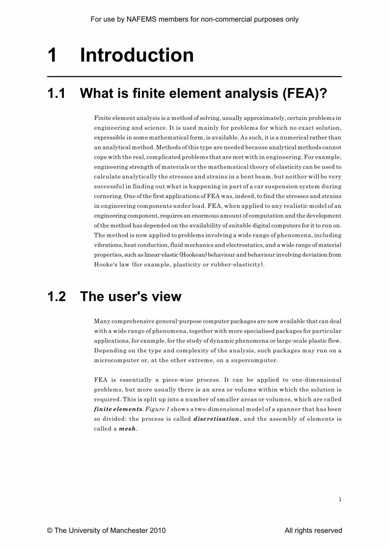
FEA is essentially a piece-wise process. It can be applied to one-dimensional

problems, but more usually there is an area or volume within which the solution is

required. This is split up into a number of smaller areas or volumes, which are called

finite elements. Figure 1 shows a two-dimensional model of a spanner that has been

so divided: the process is called discretisation, and the assembly of elements is

called a mesh.



Introduction

2

Figure 1 : Spanner divided into a number of finite elements.

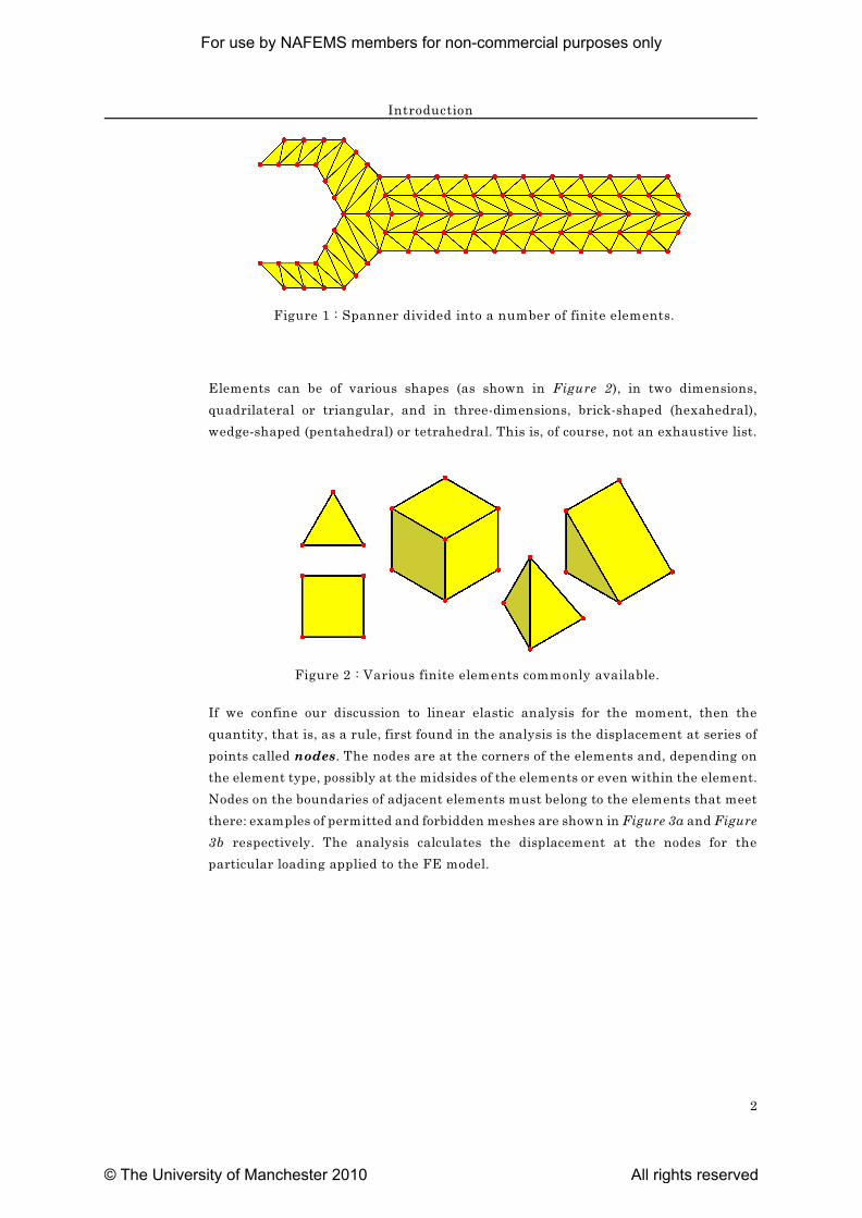
Figure 2 : Various finite elements commonly available.

Elements can be of various shapes (as shown in Figure 2), in two dimensions,

quadrilateral or triangular, and in three-dimensions, brick-shaped (hexahedral),

wedge-shaped (pentahedral) or tetrahedral. This is, of course, not an exhaustive list.

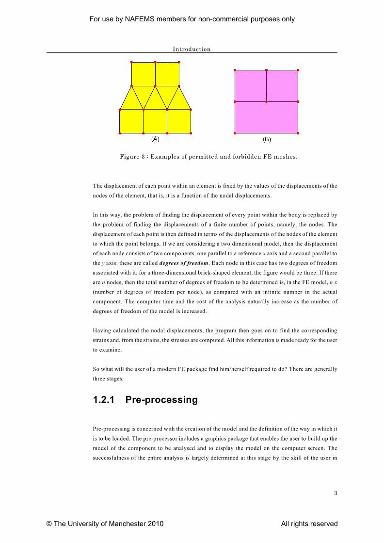
If we confine our discussion to linear elastic analysis for the moment, then the

quantity, that is, as a rule, first found in the analysis is the displacement at series of

points called nodes. The nodes are at the corners of the elements and, depending on

the element type, possibly at the midsides of the elements or even within the element.

Nodes on the boundaries of adjacent elements must belong to the elements that meet

there: examples of permitted and forbidden meshes are shown in Figure 3a and Figure

3b respectively. The analysis calculates the displacement at the nodes for the

particular loading applied to the FE model.



Introduction

3

Figure 3 : Examples of permitted and forbidden FE meshes.

The displacement of each point within an element is fixed by the values of the displacements of the

nodes of the element, that is, it is a function of the nodal displacements.

In this way, the problem of finding the displacement of every point within the body is replaced by

the problem of finding the displacements of a finite number of points, namely, the nodes. The

displacement of each point is then defined in terms of the displacements of the nodes of the element

to which the point belongs. If we are considering a two dimensional model, then the displacement

of each node consists of two components, one parallel to a reference x axis and a second parallel to

the y axis: these are called degrees of freedom . Each node in this case has two degrees of freedom

associated with it: for a three-dimensional brick-shaped element, the figure would be three. If there

are n nodes, then the total number of degrees of freedom to be determined is, in the FE model, n x

(number of degrees of freedom per node), as compared with an infinite number in the actual

component. The computer time and the cost of the analysis naturally increase as the number of

degrees of freedom of the model is increased.

Having calculated the nodal displacements, the program then goes on to find the corresponding

strains and, from the strains, the stresses are computed. All this information is made ready for the user

to examine.

So what will the user of a modern FE package find him/herself required to do? There are generally

three stages.

1.2.1 Pre-processing

Pre-processing is concerned with the creation of the model and the definition of the way in which it

is to be loaded. The pre-processor includes a graphics package that enables the user to build up the

model of the component to be analysed and to display the model on the computer screen. The

successfulness of the entire analysis is largely determined at this stage by the skill of the user in



Introduction

4

determining what simplifications (if any) are to be introduced into the model as compared with the

`real thing' and by the choice of the mesh and type of element to be used. Appropriate mechanical

or physical properties must be allocated to the material of which the model is made and loads and

possibly any restriction to the movement of certain nodes (restraints) must be applied.

The geometrical and other data produced by the pre-processor go into an input file (or deck, a term

left over from the days when the input to a computer was in the form of a stack or deck of punched

cards). It may be necessary to add to the input file other information about the way in which the

analysis is to be carried out and about the type of output (results) required: for example, are the

stresses to be determined throughout the model or - which would reduce the computing time and cost

- only in a few selected elements? When the input file is complete it is then submitted for analysis.

It is, of course, possible to produce the input file without the use of pre-processor if the model is

particularly simple. In other cases, if the software permits, the geometric information for the model

may be taken in by the pre-processor from a CAD (computer-aided design) package.

1.2.2 Analysis

The analysis part of the FE package takes in the input file, carries out certain checks on the

information contained therein and then, if there are no errors in the input file, the analysis is carried

out and output files are produced. These contain an enormous amount of information if the analysis

is at all complex. These files can be examined and the relevant information extracted but, as a rule,

there is so much information that it needs to be presented to the user in a more intelligible and user-

friendly manner. This is the job of the post-processor. The pre- and post-processor are essentially the

same software package.

1.2.3 Post-processing

The post-processor takes in the information from the output files and can present it to the user in a

range of different graphical and tabular forms. For example, depending on the facilities available,

colour may be used to indicate the value of some component of stress on the surface of the

component, or contour lines of equal stress may be drawn as in Figure 4, or similar forms of display

may be produced on sections through the model.



Introduction

5

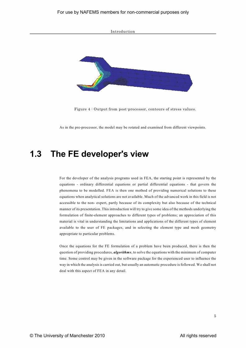
Figure 4 : Output from post-processor, contours of stress values.

As in the pre-processor, the model may be rotated and examined from different viewpoints.

1.3 The FE developer's view

For the developer of the analysis programs used in FEA, the starting point is represented by the

equations - ordinary differential equations or partial differential equations - that govern the

phenomena to be modelled. FEA is then one method of providing numerical solutions to these

equations when analytical solutions are not available. Much of the advanced work in this field is not

accessible to the non- expert, partly because of its complexity but also because of the technical

manner of its presentation. This introduction will try to give some idea of the methods underlying the

formulation of finite-element approaches to different types of problems; an appreciation of this

material is vital in understanding the limitations and applications of the different types of element

available to the user of FE packages, and in selecting the element type and mesh geometry

appropriate to particular problems.

Once the equations for the FE formulation of a problem have been produced, there is then the

question of providing procedures, algorithms, to solve the equations with the minimum of computer

time. Some control may be given in the software package for the experienced user to influence the

way in which the analysis is carried out, but usually an automatic procedure is followed. We shall not

deal with this aspect of FEA in any detail.



6

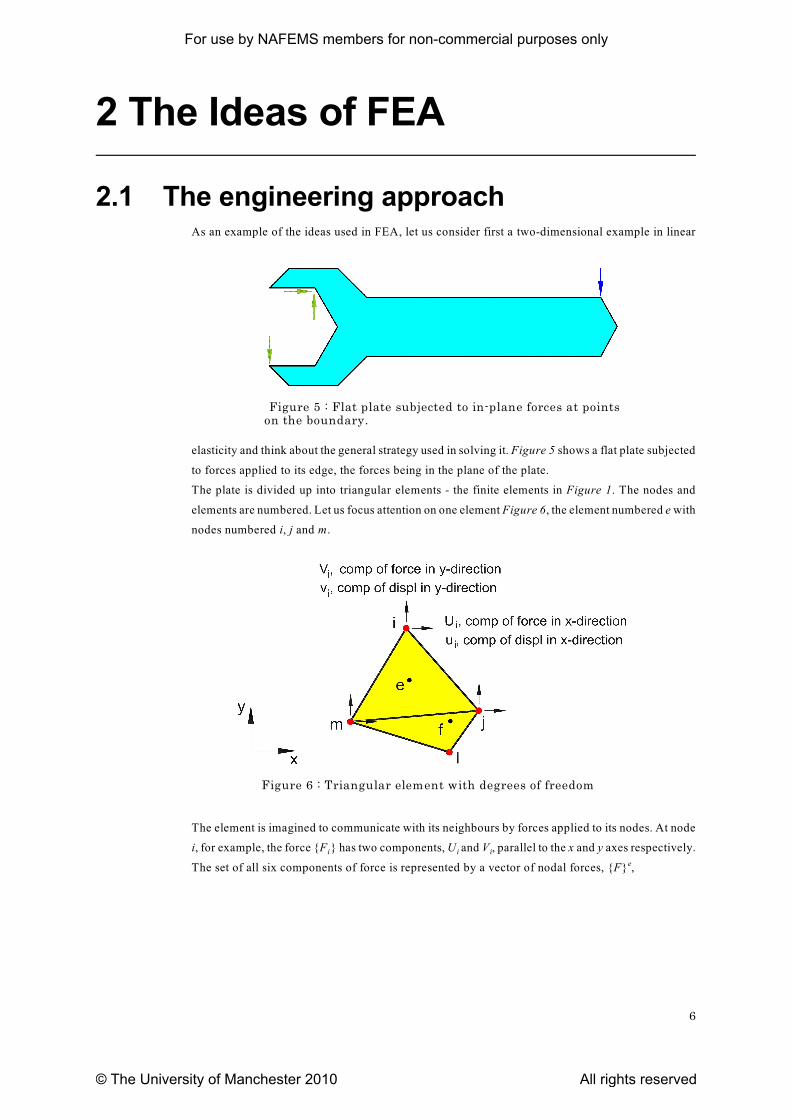
Figure 5 : Flat plate subjected to in-plane forces at pointson the boundary.

Figure 6 : Triangular element with degrees of freedom

2 The Ideas of FEA

2.1 The engineering approachAs an example of the ideas used in FEA, let us consider first a two-dimensional example in linear

elasticity and think about the general strategy used in solving it. Figure 5 shows a flat plate subjected

to forces applied to its edge, the forces being in the plane of the plate.

The plate is divided up into triangular elements - the finite elements in Figure 1. The nodes and

elements are numbered. Let us focus attention on one element Figure 6, the element numbered e with

nodes numbered i, j and m.

The element is imagined to communicate with its neighbours by forces applied to its nodes. At node

i i ii, for example, the force {F } has two components, U and V , parallel to the x and y axes respectively.

The set of all six components of force is represented by a vector of nodal forces, {F} ,e



The Ideas of FEA

7

(1)

where,

(2)

and so on, so that,

(3)

Similarly, the displacement of each node has two components, u and v, displacement of node i

i iparallel to the x-axis being denoted by u and that parallel to the y-axis by v . There is thus a vector

of nodal displacements, {ä} :e

(4)

where,

(5)

and so on, so that,



The Ideas of FEA

8

(6)

The nodal forces are dependent on the strains produced in the element by the movement of the nodes.

Of course, if all the nodes are displaced by the same vector, then the element is merely translated

without strain, and the nodal forces are zero. Similarly, if the movement reduces to a rotation without

strain, the nodal forces are also zero. The mechanical properties of the material of which the element

is made are needed to make the transition from nodal displacements to nodal forces. We shall go

through the derivation in more detail later, but at this stage we shall just state the result that the nodal

forces may be related to the nodal displacements by using a 6x6 matrix, called the element stiffness

matrix, [K] ,e

(7)

or,

(8)

The dotted lines show the partitioning of the 6x6 element stiffness matrix into nine 2x2 submatrices,

so that,

(9)

where,



The Ideas of FEA

9

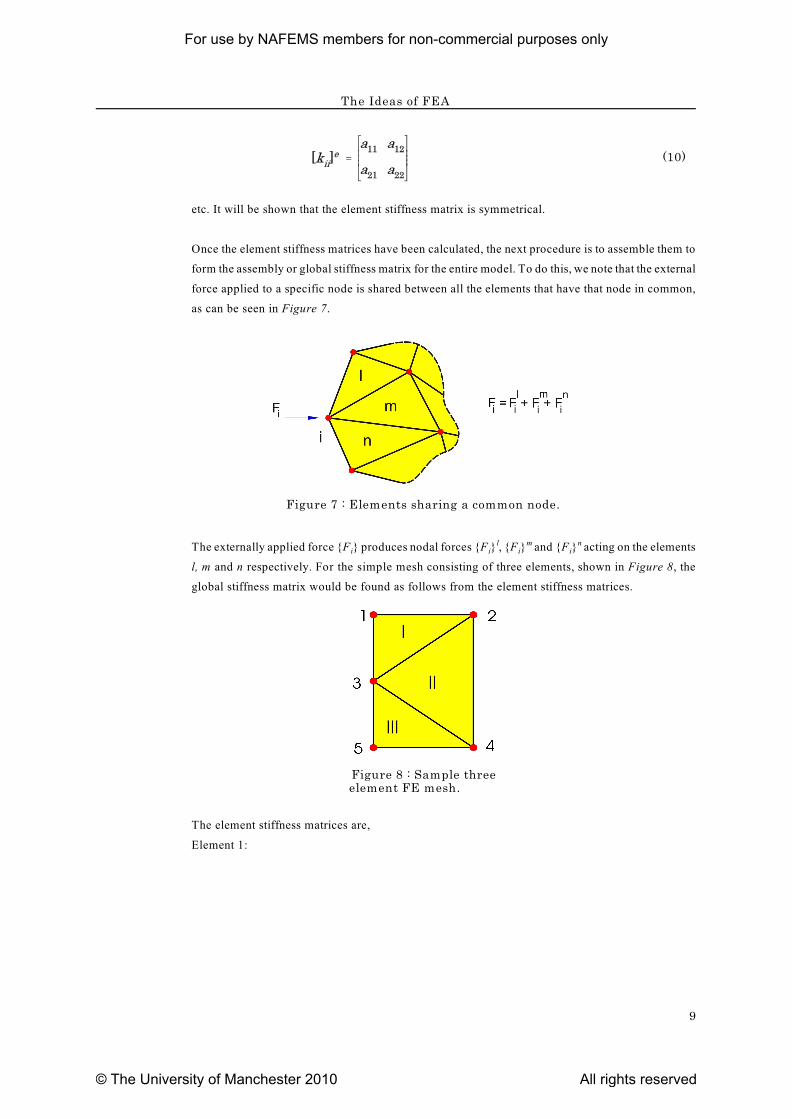
Figure 7 : Elements sharing a common node.

Figure 8 : Sample threeelement FE mesh.

(10)

etc. It will be shown that the element stiffness matrix is symmetrical.

Once the element stiffness matrices have been calculated, the next procedure is to assemble them to

form the assembly or global stiffness matrix for the entire model. To do this, we note that the external

force applied to a specific node is shared between all the elements that have that node in common,

as can be seen in Figure 7.

i i i iThe externally applied force {F } produces nodal forces {F } , {F } and {F } acting on the elementsl m n

l, m and n respectively. For the simple mesh consisting of three elements, shown in Figure 8, the

global stiffness matrix would be found as follows from the element stiffness matrices.

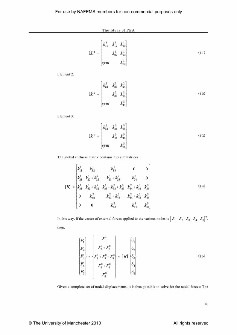
The element stiffness matrices are,

Element 1:



The Ideas of FEA

10

(11)

Element 2:

(12)

Element 3:

(13)

The global stiffness matrix contains 5x5 submatrices.

(14)

In this way, if the vector of external forces applied to the various nodes is ,

then,

(15)

Given a complete set of nodal displacements, it is thus possible to solve for the nodal forces: The



The Ideas of FEA

11

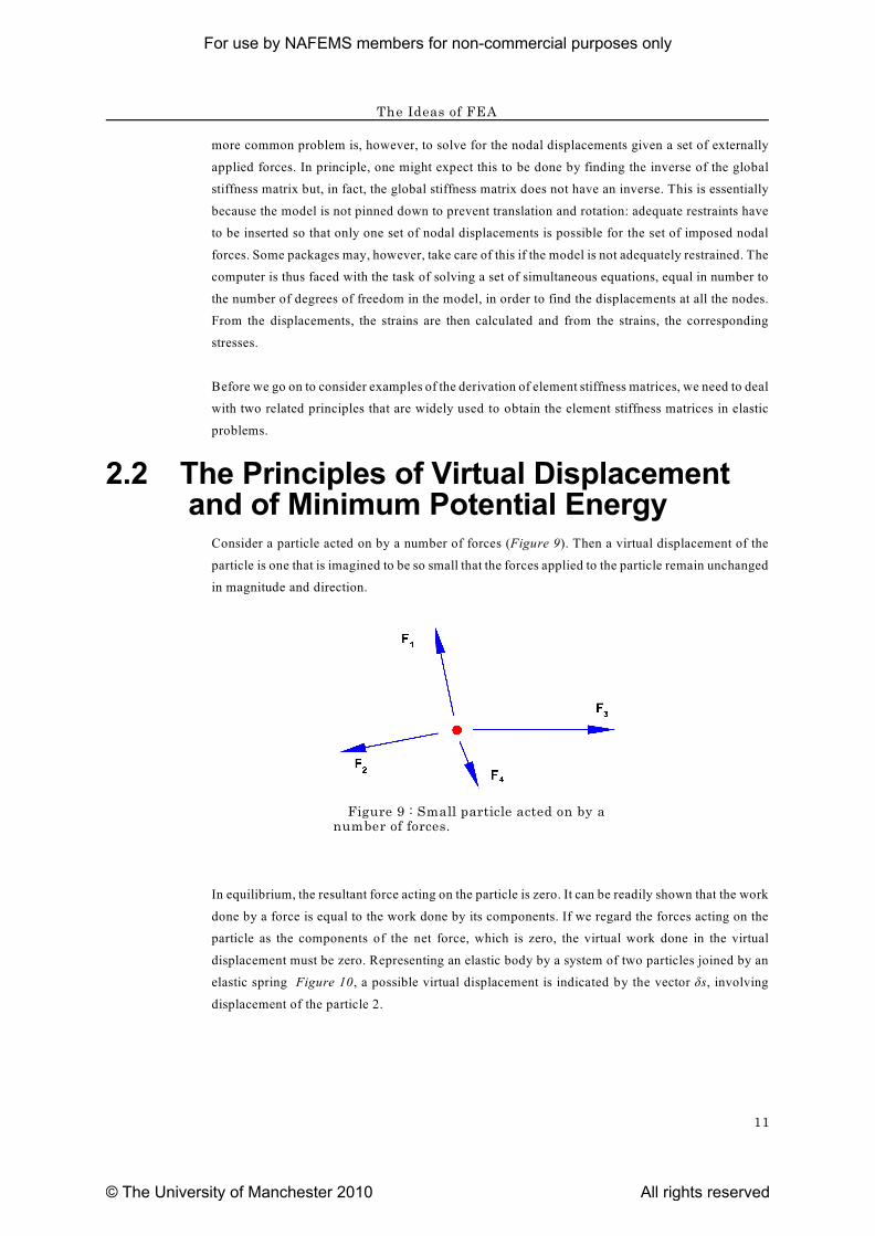
Figure 9 : Small particle acted on by anumber of forces.

more common problem is, however, to solve for the nodal displacements given a set of externally

applied forces. In principle, one might expect this to be done by finding the inverse of the global

stiffness matrix but, in fact, the global stiffness matrix does not have an inverse. This is essentially

because the model is not pinned down to prevent translation and rotation: adequate restraints have

to be inserted so that only one set of nodal displacements is possible for the set of imposed nodal

forces. Some packages may, however, take care of this if the model is not adequately restrained. The

computer is thus faced with the task of solving a set of simultaneous equations, equal in number to

the number of degrees of freedom in the model, in order to find the displacements at all the nodes.

From the displacements, the strains are then calculated and from the strains, the corresponding

stresses.

Before we go on to consider examples of the derivation of element stiffness matrices, we need to deal

with two related principles that are widely used to obtain the element stiffness matrices in elastic

problems.

2.2 The Principles of Virtual Displacement and of Minimum Potential Energy

Consider a particle acted on by a number of forces (Figure 9). Then a virtual displacement of the

particle is one that is imagined to be so small that the forces applied to the particle remain unchanged

in magnitude and direction.

In equilibrium, the resultant force acting on the particle is zero. It can be readily shown that the work

done by a force is equal to the work done by its components. If we regard the forces acting on the

particle as the components of the net force, which is zero, the virtual work done in the virtual

displacement must be zero. Representing an elastic body by a system of two particles joined by an

elastic spring Figure 10, a possible virtual displacement is indicated by the vector äs, involving

displacement of the particle 2.



The Ideas of FEA

12

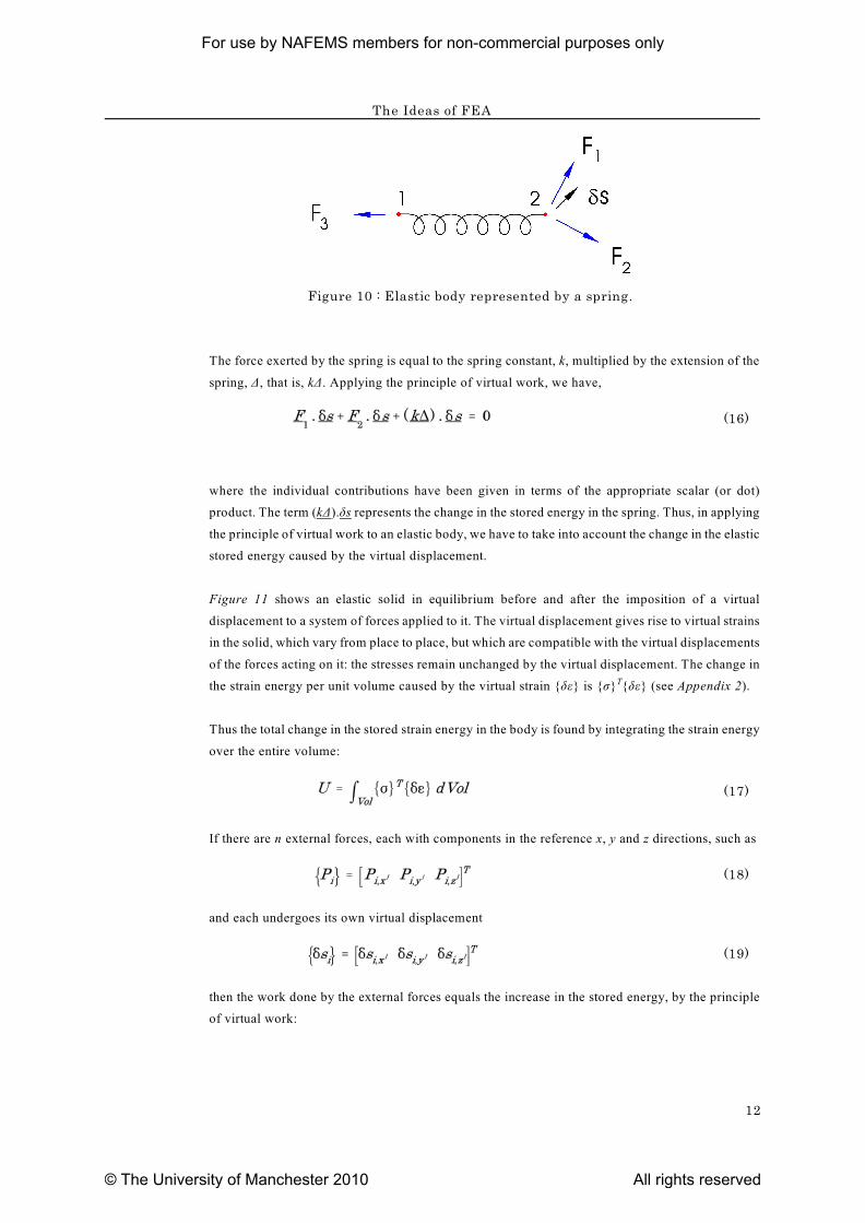
Figure 10 : Elastic body represented by a spring.

The force exerted by the spring is equal to the spring constant, k, multiplied by the extension of the

spring, Ä, that is, kÄ. Applying the principle of virtual work, we have,

(16)

where the individual contributions have been given in terms of the appropriate scalar (or dot)

product. The term (kÄ).äs represents the change in the stored energy in the spring. Thus, in applying

the principle of virtual work to an elastic body, we have to take into account the change in the elastic

stored energy caused by the virtual displacement.

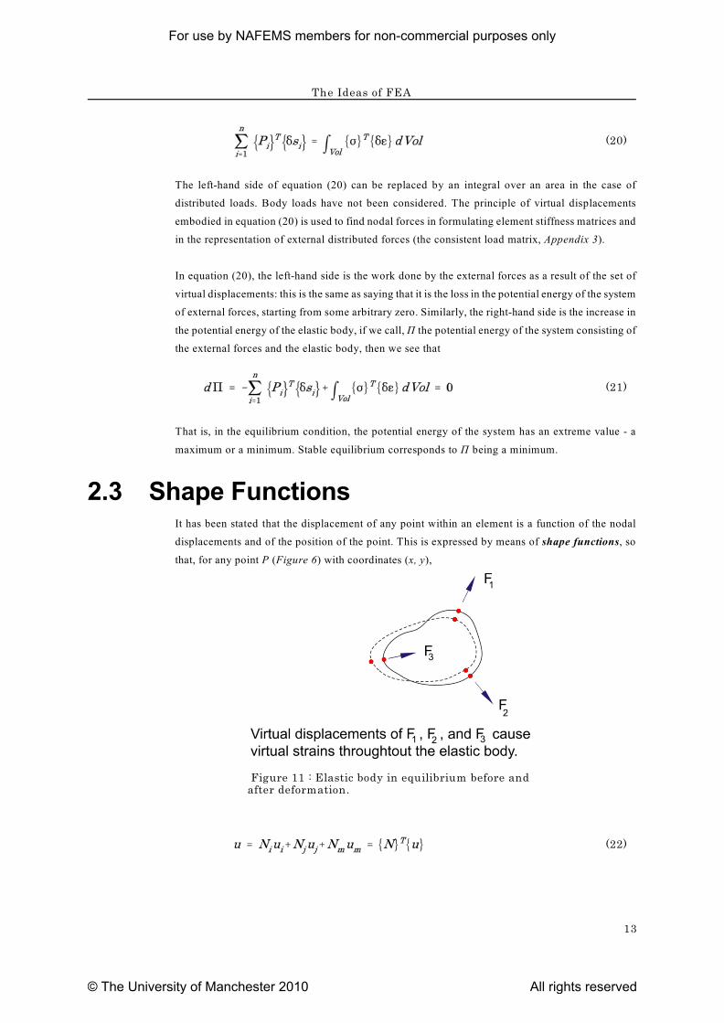
Figure 11 shows an elastic solid in equilibrium before and after the imposition of a virtual

displacement to a system of forces applied to it. The virtual displacement gives rise to virtual strains

in the solid, which vary from place to place, but which are compatible with the virtual displacements

of the forces acting on it: the stresses remain unchanged by the virtual displacement. The change in

the strain energy per unit volume caused by the virtual strain {äå} is {ó} {äå} (see Appendix 2). T

Thus the total change in the stored strain energy in the body is found by integrating the strain energy

over the entire volume:

(17)

If there are n external forces, each with components in the reference x, y and z directions, such as

(18)

and each undergoes its own virtual displacement

(19)

then the work done by the external forces equals the increase in the stored energy, by the principle

of virtual work:



The Ideas of FEA

13

Figure 11 : Elastic body in equilibrium before andafter deformation.

(20)

The left-hand side of equation (20) can be replaced by an integral over an area in the case of

distributed loads. Body loads have not been considered. The principle of virtual displacements

embodied in equation (20) is used to find nodal forces in formulating element stiffness matrices and

in the representation of external distributed forces (the consistent load matrix, Appendix 3).

In equation (20), the left-hand side is the work done by the external forces as a result of the set of

virtual displacements: this is the same as saying that it is the loss in the potential energy of the system

of external forces, starting from some arbitrary zero. Similarly, the right-hand side is the increase in

the potential energy of the elastic body, if we call, Ð the potential energy of the system consisting of

the external forces and the elastic body, then we see that

(21)

That is, in the equilibrium condition, the potential energy of the system has an extreme value - a

maximum or a minimum. Stable equilibrium corresponds to Ð being a minimum.

2.3 Shape FunctionsIt has been stated that the displacement of any point within an element is a function of the nodal

displacements and of the position of the point. This is expressed by means of shape functions, so

that, for any point P (Figure 6) with coordinates (x, y),

(22)



The Ideas of FEA

14

where,

(23)

and,

(24)

Each shape function is a function of position, .

What conditions must shape functions fulfil?

1. At a node, we know what the displacement should be in terms of the nodal displacements:

iat node i, it is {ä }. So, for example,

(25)

iThis is true for any value that the nodal displacements may have, and so N is equal to 1 at

node i and is zero at all the other nodes. The same is true of all the other shape functions:

(26)

2. The displacement needs to be continuous at the boundary between one element and its

neighbours. In Figure 6, along the boundary jm, for example, the displacement at a point

must depend only on the nodal displacements at the ends of the boundary (and the position

i lof the point). If it were to depend on {ä } in element e, then it would also depend on {ä }

l iin element f, and since, in general, {ä } � {ä }, the displacement would not be continuous

iacross the boundary. So The shape function, N must be zero along the boundary jm, and

j msimilarly for N and N along the boundaries im and ij respectively. The shape function

corresponding to a node is thus zero along a boundary not including that node.

3. The shape functions should be able to represent translation,

(27)

without distortion. All points in the element should be displaced by the same amount as the

nodes,

(28)

But,

(29)



The Ideas of FEA

15

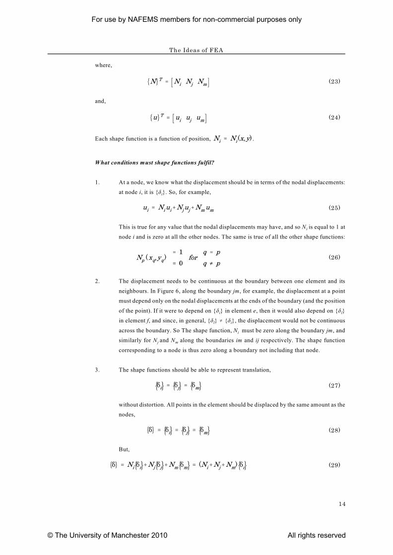
Figure 12 : Point subjected to a small rotation

i j mThis condition requires that N + N + N = 1 for all points in the element.

4. The shape functions should be able to represent rotation without distortion. Figure 12

shows the point P with coordinates (x, y) subjected to a small rotation about the origin,

causing it to move through a distance rè.

The component of the displacement in the x direction, u, is given by,

(30)

and since

(31)

equation (30) can be written as

(32)

Similarly for the nodal displacements:

(33)

By substituting these values into equation (22), we obtain

(34)

Hence by making use of equation (33),

(35)

and similarly,



The Ideas of FEA

16

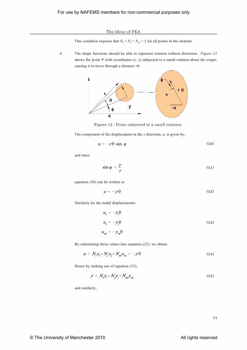
Figure 13 : Area shape functions for atriangular element.

(36)

For the triangular element, suitable shape functions are the so-called area shape functions (Figure

13): for example,

(37)

i j mThe shape functions N , N and N clearly satisfy the first three conditions given above, and it can also

be shown that they satisfy the fourth.

2.4 Relationship between displacementand strain

x y xyIt can be shown (see Appendix 1) that the strains å , å and ã at any

point in a two-dimensional state of strain are given by:

(38)



The Ideas of FEA

17

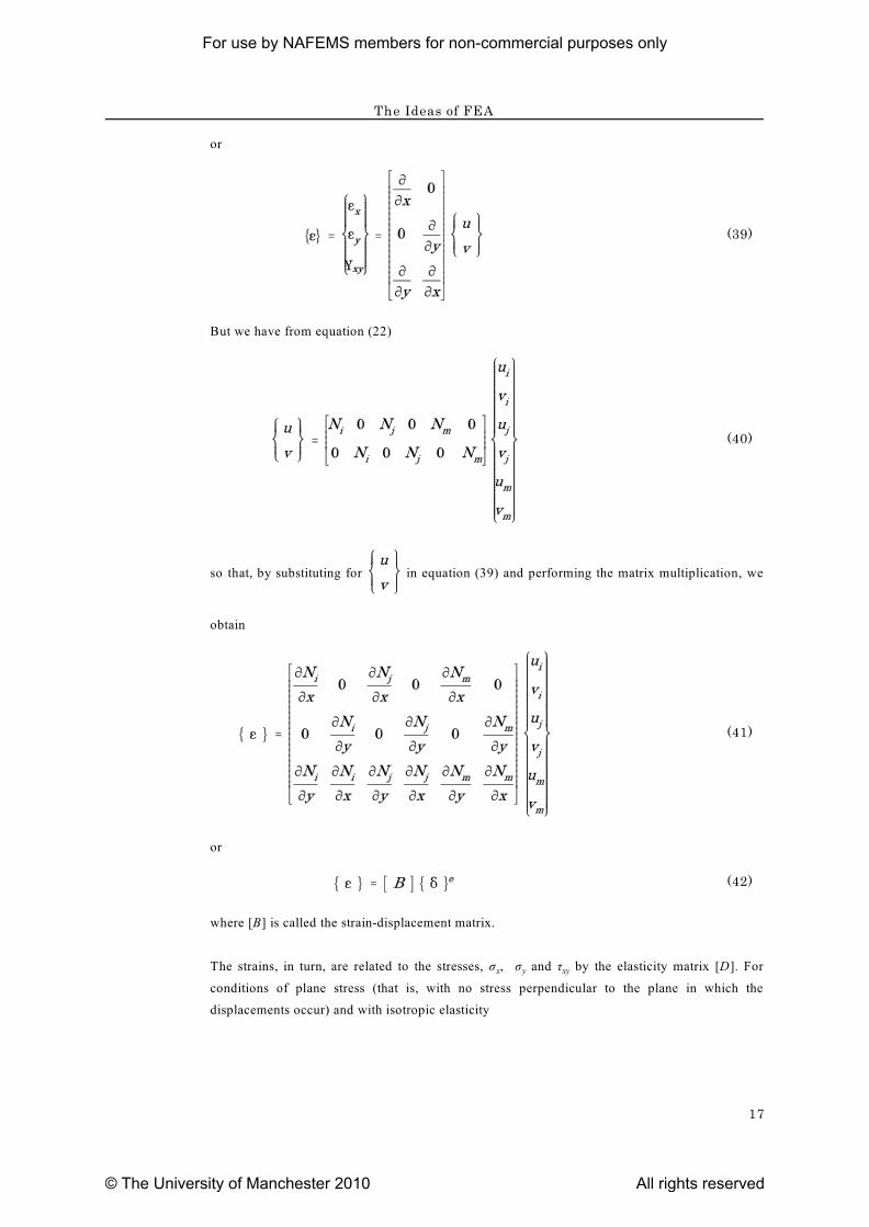
or

(39)

But we have from equation (22)

(40)

so that, by substituting for in equation (39) and performing the matrix multiplication, we

obtain

(41)

or

(42)

where [B] is called the strain-displacement matrix.

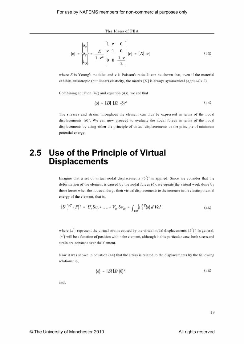
x y xyThe strains, in turn, are related to the stresses, ó , ó and ô by the elasticity matrix [D]. For

conditions of plane stress (that is, with no stress perpendicular to the plane in which the

displacements occur) and with isotropic elasticity



The Ideas of FEA

18

(43)

where E is Young's modulus and í is Poisson's ratio. It can be shown that, even if the material

exhibits anisotropic (but linear) elasticity, the matrix [D] is always symmetrical (Appendix 2).

Combining equation (42) and equation (43), we see that

(44)

The stresses and strains throughout the element can thus be expressed in terms of the nodal

displacements {ä} . We can now proceed to evaluate the nodal forces in terms of the nodale

displacements by using either the principle of virtual displacements or the principle of minimum

potential energy.

2.5 Use of the Principle of VirtualDisplacements

Imagine that a set of virtual nodal displacements {ä } is applied. Since we consider that the* e

deformation of the element is caused by the nodal forces (6), we equate the virtual work done by

these forces when the nodes undergo their virtual displacements to the increase in the elastic potential

energy of the element, that is,

(45)

where {å } represent the virtual strains caused by the virtual nodal displacements {ä } . In general,* * e

{å } will be a function of position within the element, although in this particular case, both stress and*

strain are constant over the element.

Now it was shown in equation (44) that the stress is related to the displacements by the following

relationship,

(46)

and,



The Ideas of FEA

19

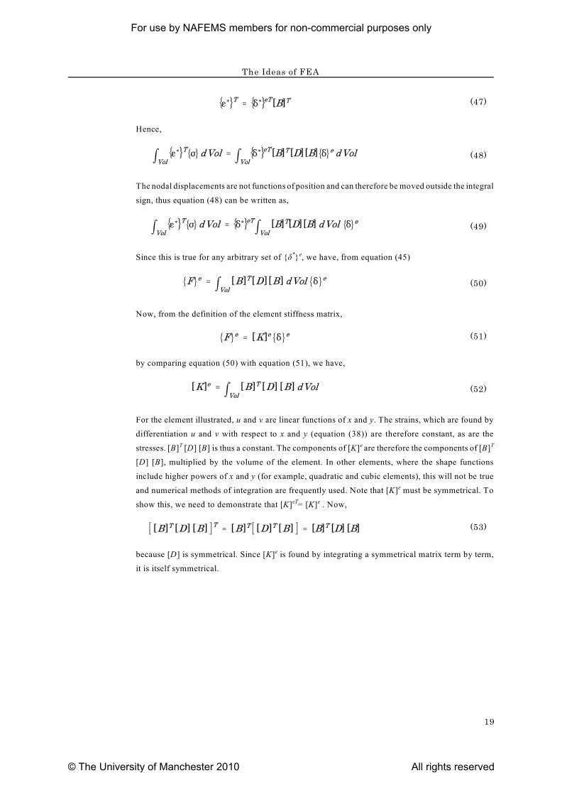
(47)

Hence,

(48)

The nodal displacements are not functions of position and can therefore be moved outside the integral

sign, thus equation (48) can be written as,

(49)

Since this is true for any arbitrary set of {ä } , we have, from equation (45)* e

(50)

Now, from the definition of the element stiffness matrix,

(51)

by comparing equation (50) with equation (51), we have,

(52)

For the element illustrated, u and v are linear functions of x and y. The strains, which are found by

differentiation u and v with respect to x and y (equation (38)) are therefore constant, as are the

stresses. [B] [D] [B] is thus a constant. The components of [K] are therefore the components of [B]T e T

[D] [B], multiplied by the volume of the element. In other elements, where the shape functions

include higher powers of x and y (for example, quadratic and cubic elements), this will not be true

and numerical methods of integration are frequently used. Note that [K] must be symmetrical. Toe

show this, we need to demonstrate that [K] = [K] . Now,eT e

(53)

because [D] is symmetrical. Since [K] is found by integrating a symmetrical matrix term by term,e

it is itself symmetrical.



The Ideas of FEA

20

2.6 Use of the Principle of MinimumPotential Energy

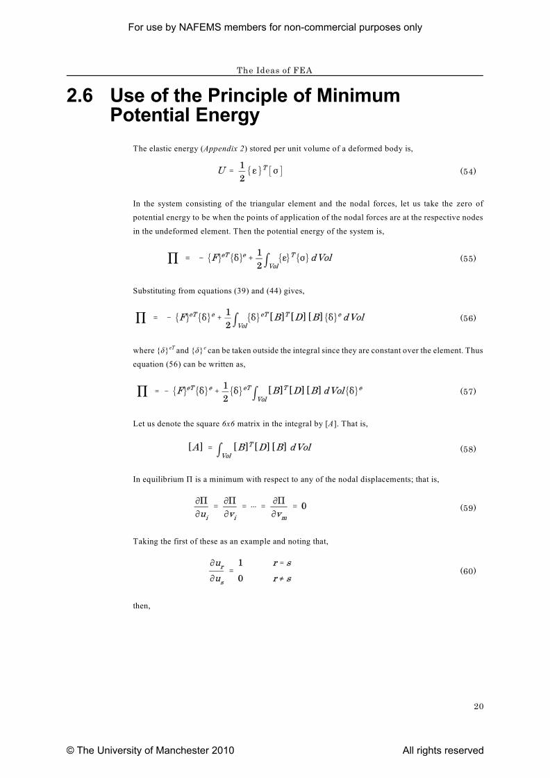
The elastic energy (Appendix 2) stored per unit volume of a deformed body is,

(54)

In the system consisting of the triangular element and the nodal forces, let us take the zero of

potential energy to be when the points of application of the nodal forces are at the respective nodes

in the undeformed element. Then the potential energy of the system is,

(55)

Substituting from equations (39) and (44) gives,

(56)

where {ä} and {ä} can be taken outside the integral since they are constant over the element. ThuseT e

equation (56) can be written as,

(57)

Let us denote the square 6x6 matrix in the integral by [A]. That is,

(58)

In equilibrium Ð is a minimum with respect to any of the nodal displacements; that is,

(59)

Taking the first of these as an example and noting that,

(60)

then,



The Ideas of FEA

21

(61)

which can be written explicitly as,

(62)

It has been noted in Section 2.5 that [A] is symmetrical and the last two terms in equation (61) are

therefore equal, so that,

(63)

and, in general,

(64)

By comparing this with equation (51), we see that,

(65)

and the same result is, of course, obtained as by use of the method of virtual displacement (equation

(52)).

In this particular case of the uniform-strain triangular element, since the integrand in equation (64)

is a constant, equation (65) may be written as

(66)

where Ä is the area of the triangular element and t is its thickness.



22

3 Variational and Weighted

Residual Methods

3.1 Introduction

In Section 2, an approach based on the ideas employed in solid mechanics was used to indicate how

the stiffness matrix could be derived for a linear elastic element, and how such matrices could be

assembled to represent an entire body. As a result, a global stiffness matrix is obtained that relates

the nodal displacements to the applied nodal forces.

The finite-element method is not, however, confined to problems in applied mechanics: it can also

be used to solve steady-state field problems (for example, involving a temperature distribution) as

well as time-dependent problems (for example, the approach to a transient temperature distribution).

It is with the first of these two types of problem that we shall be concerned in this section.

Let us imagine that the problem that we wish to solve is one involving a two-dimensional steady-state

temperature distribution: that is, there is one dimension, z, along which temperature does not vary.

Suppose that the temperature distribution is given on the boundary Ã of a certain region, Ù, and we

know the rate at which heat is being supplied at all positions in Ù. Our task is to find the temperature

distribution throughout Ù. (Other types of boundary condition may be specified, for example, the rate

at which heat is flowing into or out of the region across part of the boundary may be fixed). Then if

{ö} is the vector of nodal temperatures and Q is a function defining the heat input, then we seek a

matrix expression such that

(67)

which gives a system of simultaneous equations that may be solved to find {ö}. By analogy with the

nomenclature first used in stress analysis, the matrix [K] is called the stiffness matrix. The column

matrix {f} depends on Q and may incorporate certain of the boundary conditions.

3.2 Governing equations for physicalproblems

In order to solve the steady-state heat flow problem posed above, we must have some underlying

equation that, together with the boundary conditions, must be satisfied by the solution. For the

conduction of heat in one dimension,



Variational and Weighted Residual Methods

23

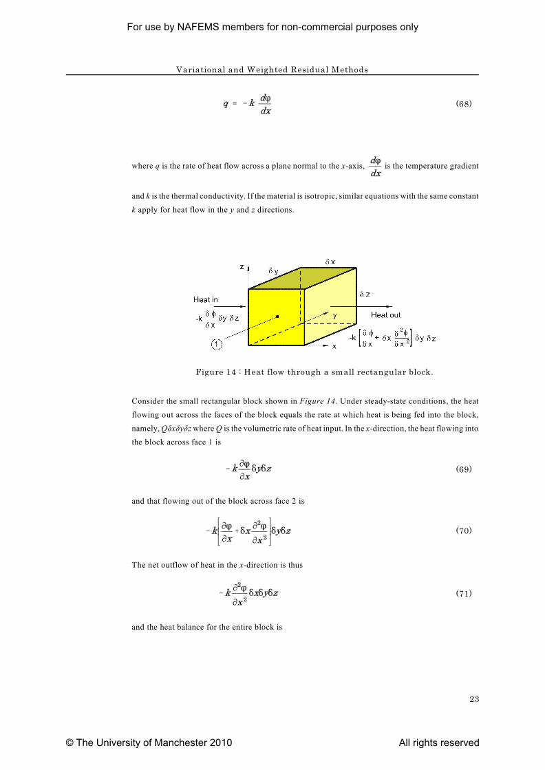
Figure 14 : Heat flow through a small rectangular block.

(68)

where q is the rate of heat flow across a plane normal to the x-axis, is the temperature gradient

and k is the thermal conductivity. If the material is isotropic, similar equations with the same constant

k apply for heat flow in the y and z directions.

Consider the small rectangular block shown in Figure 14. Under steady-state conditions, the heat

flowing out across the faces of the block equals the rate at which heat is being fed into the block,

namely, Qäxäyäz where Q is the volumetric rate of heat input. In the x-direction, the heat flowing into

the block across face 1 is

(69)

and that flowing out of the block across face 2 is

(70)

The net outflow of heat in the x-direction is thus

(71)

and the heat balance for the entire block is




24

(72)

or

(73)

Equation (73) is the governing partial differential equation for the steady-state conduction of heat

in an isotropic body. Governing equations that are, of course, different in form, apply to other

physical phenomena, for example, gravitational fields, electrostatic fields, fluid flow (potential flow)

etc.

3.3 Variational Methods

In the previous section, we have tried to show, with steady-state heat conduction as an example, that

the solution of many problems in science and engineering involves the solution of a governing

equation: that is, an equation (usually a partial differential equation), which is subject to certain

boundary conditions. Variational methods, on the other hand, approach the problem in a different

way. In a steady-state heat conduction problem in two dimensions, the solution is a temperature

distribution ö(x, y). This distribution is that that makes a certain integral over the region to which it

applies take on an extreme value. An integral of this type is called a functional, and the branch of

mathematics concerned with variational methods is called the Calculus of Variations.

The functional often embodies some physical principle: for example, in elastic problems it is the

potential energy of the deformed body and of the forces acting on the body. In this case, the

functional takes on a minimum value at equilibrium and the use of variational methods is equivalent

to the use of the principle of virtual work.

It can be shown that, for any functional, there is a corresponding equation - the Euler equation - the

solution of which, subject to the appropriate boundary conditions, gives rise to stationarity of the

functional (that is, the functional has an extreme value, usually a maximum or a minimum). The

reverse is not true: that is, a functional cannot always be found to correspond to a particular

governing equation.

As an example, consider the functional:

(74)




25

0 Lwhich is to be made stationary, subject to the following conditions: ö= ö at x = 0 and ö = ö at x =

L. k is a constant: Q is a given function of position, x, and ö is to be determined in the range 0<x<L

so that Ð(ö) should be stationary.

If Ð(ö) is stationary when ö(x)= u(x), then any small permissible change in ö, that is, a change that

is consistent with the boundary conditions, will cause a change in Ð(ö) that will tend to zero as the

magnitude in the change in ö decreases. This is called the first variation in Ð(ö), äÐ(ö) and so äÐ(ö)

= 0 is merely an alternative way of expressing the requirement of stationarity. The variation away

from u(x), that is, away from the value of ö giving rise to the extremum of the functional, is expressed

as åç(x), where å is a number and ç(x) is a function of x satisfying the conditions ç(0) = ç(L) = 0.

Then

(75)

and the condition of stationarity to be satisfied is that

(76)

when å = 0.

Differentiating under the integral sign, we obtain:

(77)

and hence:

(78)

Evaluating the first term by integration by parts and noting that ç(0) = ç(L) = 0, we have:

(79)

Hence




26

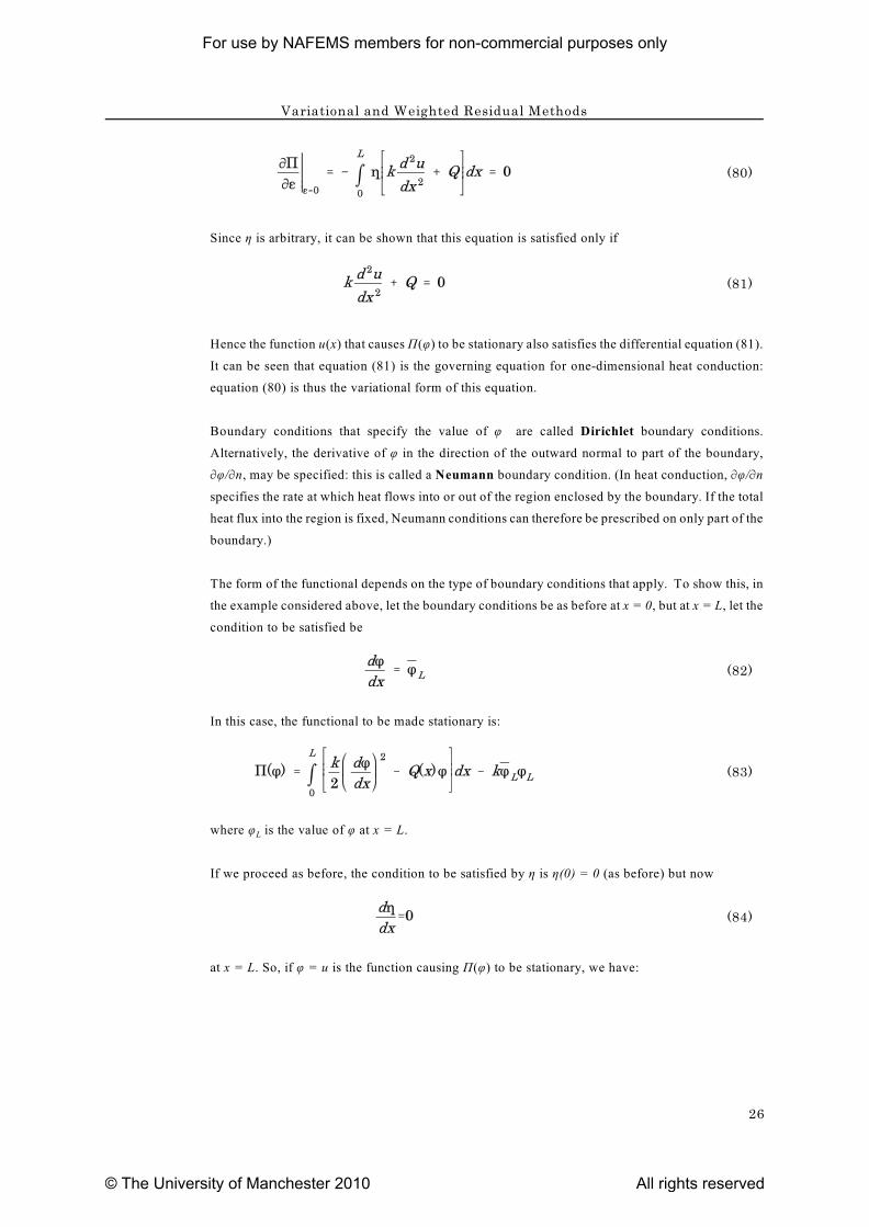
(80)

Since ç is arbitrary, it can be shown that this equation is satisfied only if

(81)

Hence the function u(x) that causes Ð(ö) to be stationary also satisfies the differential equation (81).

It can be seen that equation (81) is the governing equation for one-dimensional heat conduction:

equation (80) is thus the variational form of this equation.

Boundary conditions that specify the value of ö are called Dirichlet boundary conditions.

Alternatively, the derivative of ö in the direction of the outward normal to part of the boundary,

Mö/Mn, may be specified: this is called a Neumann boundary condition. (In heat conduction, Mö/Mn

specifies the rate at which heat flows into or out of the region enclosed by the boundary. If the total

heat flux into the region is fixed, Neumann conditions can therefore be prescribed on only part of the

boundary.)

The form of the functional depends on the type of boundary conditions that apply. To show this, in

the example considered above, let the boundary conditions be as before at x = 0, but at x = L, let the

condition to be satisfied be

(82)

In this case, the functional to be made stationary is:

(83)

Lwhere ö is the value of ö at x = L.

If we proceed as before, the condition to be satisfied by ç is ç(0) = 0 (as before) but now

(84)

at x = L. So, if ö = u is the function causing Ð(ö) to be stationary, we have:




27

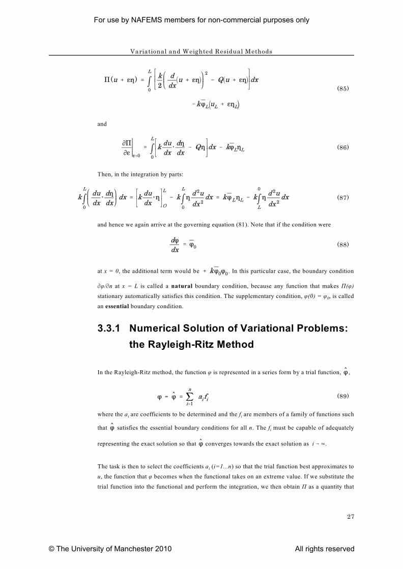
(85)

and

(86)

Then, in the integration by parts:

(87)

and hence we again arrive at the governing equation (81). Note that if the condition were

(88)

at x = 0, the additional term would be . In this particular case, the boundary condition

Mö/Mn at x = L is called a natural boundary condition, because any function that makes Ð(ö)

0stationary automatically satisfies this condition. The supplementary condition, ö(0) = ö , is called

an essential boundary condition.

3.3.1 Numerical Solution of Variational Problems:

the Rayleigh-Ritz Method

In the Rayleigh-Ritz method, the function ö is represented in a series form by a trial function, ,

(89)

i iwhere the a are coefficients to be determined and the f are members of a family of functions such

ithat satisfies the essential boundary conditions for all n. The f must be capable of adequately

representing the exact solution so that converges towards the exact solution as i 6 4.

iThe task is then to select the coefficients a (i=1...n) so that the trial function best approximates to

u, the function that ö becomes when the functional takes on an extreme value. If we substitute the

trial function into the functional and perform the integration, we then obtain Ð as a quantity that




28

1 ndepends on the coefficients a ......a .

Since Ð is required to be stationary, the derivatives of Ð with respect to any of the coefficients

1 na ......a will be zero: that is

(90)

Hence a series of n simultaneous equations is obtained from which the n coefficients can be

calculated. The procedure is illustrated by means of a simple example.

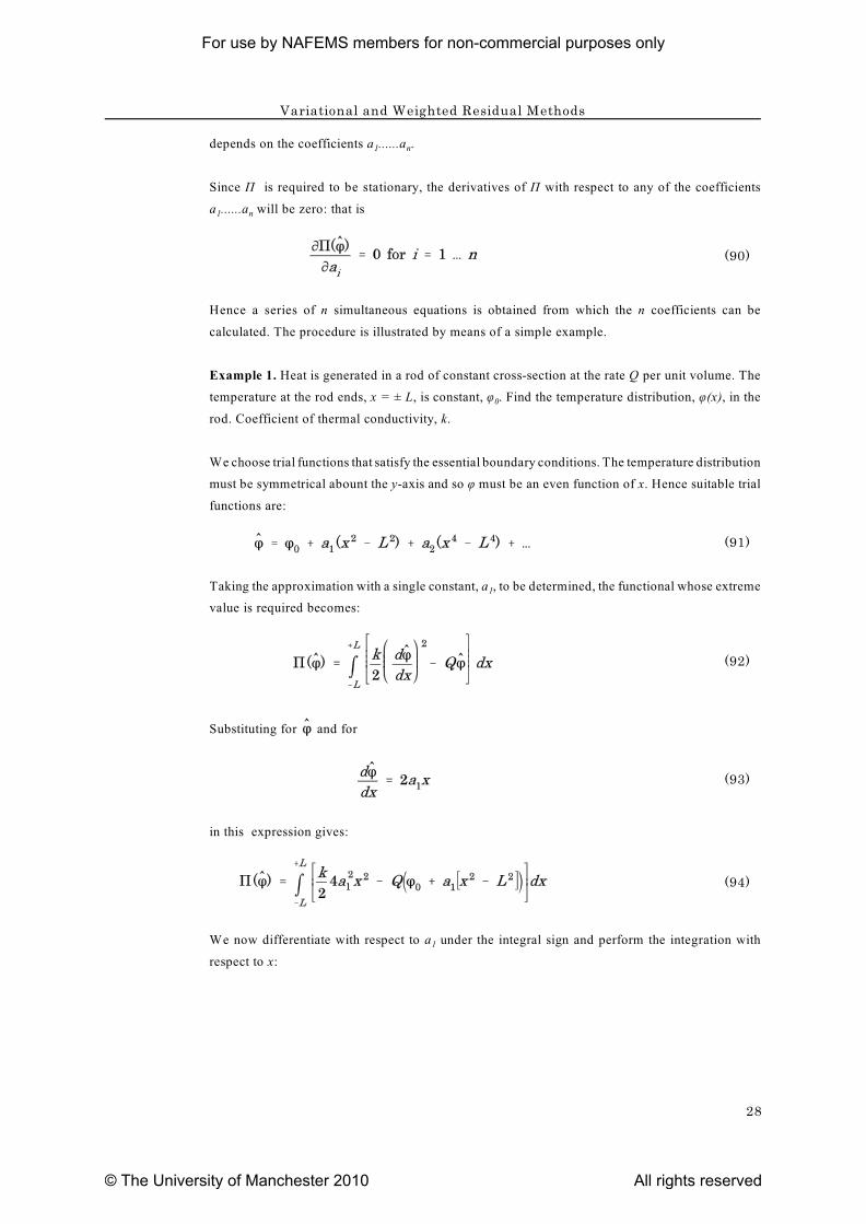
Example 1. Heat is generated in a rod of constant cross-section at the rate Q per unit volume. The

0temperature at the rod ends, x = ± L, is constant, ö . Find the temperature distribution, ö(x), in the

rod. Coefficient of thermal conductivity, k.

We choose trial functions that satisfy the essential boundary conditions. The temperature distribution

must be symmetrical abount the y-axis and so ö must be an even function of x. Hence suitable trial

functions are:

(91)

1Taking the approximation with a single constant, a , to be determined, the functional whose extreme

value is required becomes:

(92)

Substituting for and for

(93)

in this expression gives:

(94)

1We now differentiate with respect to a under the integral sign and perform the integration with

respect to x:




29

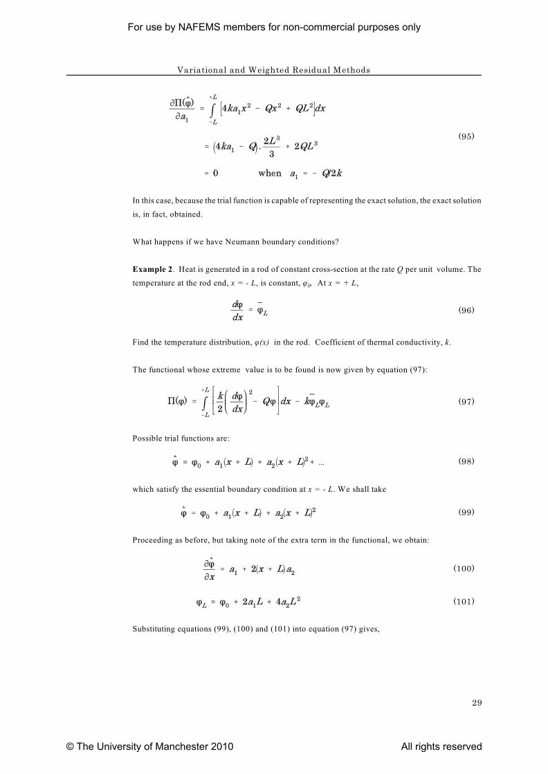
(95)

In this case, because the trial function is capable of representing the exact solution, the exact solution

is, in fact, obtained.

What happens if we have Neumann boundary conditions?

Example 2. Heat is generated in a rod of constant cross-section at the rate Q per unit volume. The

0temperature at the rod end, x = - L, is constant, ö . At x = + L,

(96)

Find the temperature distribution, ö(x) in the rod. Coefficient of thermal conductivity, k.

The functional whose extreme value is to be found is now given by equation (97):

(97)

Possible trial functions are:

(98)

which satisfy the essential boundary condition at x = - L. We shall take

(99)

Proceeding as before, but taking note of the extra term in the functional, we obtain:

(100)

(101)

Substituting equations (99), (100) and (101) into equation (97) gives,




30

(102)

1Differentiating with respect to a gives,

(103)

(* Neglecting terms in , since the integral is zero.)

The condition

(104)

gives the equation:

(105)

Similarly:

(106)

This can be written as,

(107)

Evaluating the integral gives,




31

(108)

and the condition

(109)

gives the equation,

(110)

1 2Solving equations (105) and (110) for a and a gives:

(111)

In this case again, the exact solution is obtained. Note that the boundary condition at x = + L is

automatically satisfied by the solution, in accordance with its being a natural boundary condition.

3.3.2 The Finite-Element Modification of the

Rayleigh-Ritz Method

In the Raleigh-Ritz method, a single trial function is applied throughout the entire region in which

the solution is sought. Trial functions of increasing complexity are required to realistically model all

but the simplest problems. The finite-element approach, on the other hand, uses comparatively simple

trial functions that are applied piece-wise to parts of the region. These subsections of the region are

then the finite elements. In most cases, the trial functions are required to be continuous from element

to element.

As an example, consider the problem of one dimensional heat flow. The functional to be extremised

is

(112)

where the integral over Ù corresponds to the length of the region and Neumann boundary conditions




32

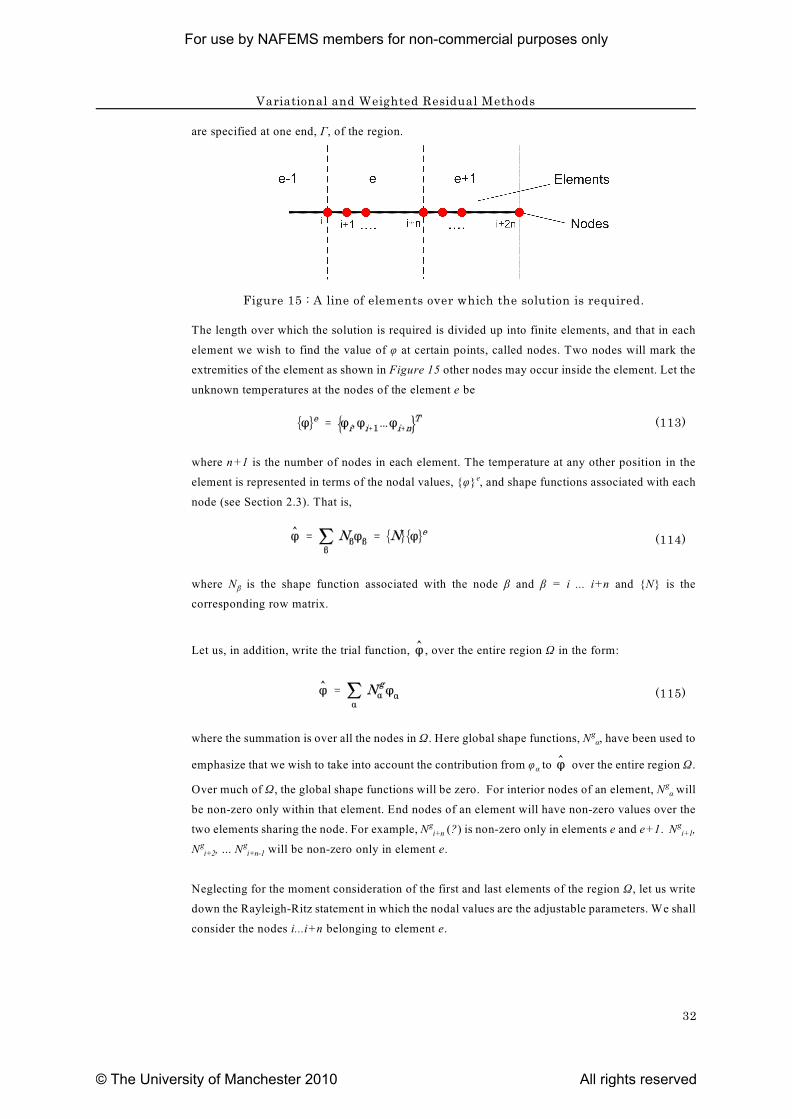
Figure 15 : A line of elements over which the solution is required.

are specified at one end, Ã, of the region.

The length over which the solution is required is divided up into finite elements, and that in each

element we wish to find the value of ö at certain points, called nodes. Two nodes will mark the

extremities of the element as shown in Figure 15 other nodes may occur inside the element. Let the

unknown temperatures at the nodes of the element e be

(113)

where n+1 is the number of nodes in each element. The temperature at any other position in the

element is represented in terms of the nodal values, {ö} , and shape functions associated with eache

node (see Section 2.3). That is,

(114)

âwhere N is the shape function associated with the node â and â = i ... i+n and {N} is the

corresponding row matrix.

Let us, in addition, write the trial function, , over the entire region Ù in the form:

(115)

áwhere the summation is over all the nodes in Ù. Here global shape functions, N , have been used tog

áemphasize that we wish to take into account the contribution from ö to over the entire region Ù.

áOver much of Ù, the global shape functions will be zero. For interior nodes of an element, N willg

be non-zero only within that element. End nodes of an element will have non-zero values over the

i+n i+1two elements sharing the node. For example, N (?) is non-zero only in elements e and e+1. N ,g g

i+2 i+n-1N , ... N will be non-zero only in element e.g g

Neglecting for the moment consideration of the first and last elements of the region Ù, let us write

down the Rayleigh-Ritz statement in which the nodal values are the adjustable parameters. We shall

consider the nodes i...i+n belonging to element e.




33

(116)

(117)

(118)

where, for example, stands for

(119)

over the element e. Since

(120)

is an expression involving the {ö} ande-1

(121)

involves {ö} and there is no relationship between {ö} and {ö} , both expresssions must be equale e-1 e

to zero.

For the moment, we shall confine attention to the terms containing an integral over the element e.

We shall drop the superfix g on the shape functions, since we are now focussing on one specific

e eelement. Let us suppose that the element extends from x=x to x=x + h. No loss in generality is

eincurred if we shift the origin to x=x and take the element to extend rather from 0 to h. Then,

(122)

We note that




34

(123)

and

(124)

since

(125)

and hence

(126)

So, differentiating under the integral sign, we have:

(127)

Hence

(128)

This equation is one in the set of n+1 simultaneous equations obtained by letting á run through the

values i...i+n:

(129)

where




35

(130)

and

(131)

In the end elements, where Neumann boundary conditions may have to be considered, there is an

additional term on the right-hand side, namely,

(132)

á,r áwhere N is the value of N on the boundary Ã.

Assembly of the element matrices is carried out as in Section 2.1. For example, if there are two two-

noded elements, labelled m and n, with nodes i , i+1 (the common node between elements m and n)

and i+2, then:

(133)

and

(134)

so that, by combining these two matrix equations:

(135)

In this way, the global assembly matrix is built up. The boundary conditions on the extreme elements

may then be inserted and the set of equations solved for the unknown values of ö.

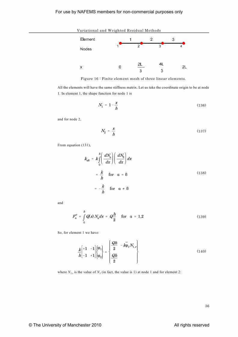
Example 3. Find an approximate solution to example 1, using three linear elements of equal length

(see Figure 16).




36

Figure 16 : Finite element mesh of three linear elements.

All the elements will have the same stiffness matrix. Let us take the coordinate origin to be at node

1. In element 1, the shape function for node 1 is

(136)

and for node 2,

(137)

From equation (131),

(138)

and

(139)

So, for element 1 we have:

(140)

1,r 1where N is the value of N (in fact, the value is 1) at node 1 and for element 2:




37

(141)

and for element 3

(142)

4,r 4where N is the value of N at node 4 (where N is, in fact, equal to 1).

Assembling the matrices, we have:

(143)

1 4 0 2 3Given ö = ö = ö ,we can solve for ö and ö from rows 2 and 3:

(144)

from which

(145)

since

(146)

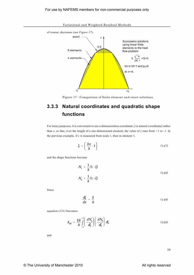
In fact, this is the same as the exact solution for the nodal values, but between the nodes the finite-

element approximation deviates from the exact solution. (The fact that the exact solution is obtained

at the nodes is called superconvergence).

As the number of elements is increased, the deviation from the exact result at the non-nodal positions,




38

Figure 17 : Comparison of finite element and exact solutions.

of course, decreases (see Figure 17).

3.3.3 Natural coordinates and quadratic shape

functions

For many purposes, it is convenient to use a dimensionless coordinate î (a natural coordinate) rather

than x, so that, over the length of a one-dimensional element, the value of î runs from +1 to -1. In

the previous example, if x is measured from node 1, then in element 1,

(147)

and the shape functions become

(148)

Since

(149)

equation (131) becomes:

(150)

and




39

(151)

The use of coordinates of this type will be found to be especially valuable in treating two- and three-

dimensional elements with curvilinear boundaries (Appendix 4).

Higher-order shape functions allow the variable to alter in a more complicated fashion - not merely

linearly - within an element. This means that, for example, fewer quadratic than linear elements are

required to represent a given physical problem with a given degree of precision, but the amount of

computation per element is increased. For many purposes, quadratic elements represent a good

compromise in requiring neither an excessive number of elements nor an excessive amount of

computation per element. There are, however, finite-element packages that employ large finite

elements and obtain results of increasing precision with an unchanged mesh by using shape functions

of increasing complexity. This is the p-approach, as opposed to the more common h-approach in

which one attempts to get better precision by mesh refinement.

Quadratic one-dimensional elements have three nodes in each element: one at each end and one in

the middle. The corresponding shape functions are:

(152)

Example 4. Obtain the element stiffness matrix for a quadratic one-dimensional element for heat

conduction and using one such element, obtain a solution to the problem of Example 1.

From equation (131), the components of the 3x3 element stiffness matrix satisfy the condition:

(153)

Now




40

(154)

Hence

(155)

and so on, so that:

(156)

Note that the matrix is symmetrical. We also need to evaluate

(157)

With Q a constant:

(158)




41

If and are the values of at x = ± L,

then the equations to be solved are:

(159)

1 3 0with ö = ö = ö .

2Expanding row 2 and solving for ö gives

(160)

2since h=2L, which, of course, is the exact solution. Substituting the value of ö and expanding row

1 enables to be found. Again the exact value is obtained,

(161)

since the quadratic finite element can exactly represent the actual quadratic variation of ö with x.

With the linear finite elements used in the previous section, it is clear that the estimate of

approaches the exact value as the number of elements is increased.

3.4 The Weighted Residual Method

Let us again take as an example the governing equation for one-dimensional heat conduction:

(162)

As in the previous section, where a solution to this equation for specific boundary conditions was

sought in terms of extremising a functional, we wish to find a solution by making use of a trial

1 2 nfunction containing a number of parameters, a , a .... a , to be determined. In general, the trial

function will not exactly satisfy equation (145) at all points in the region Ù in which the solution is

sought: that is,




42

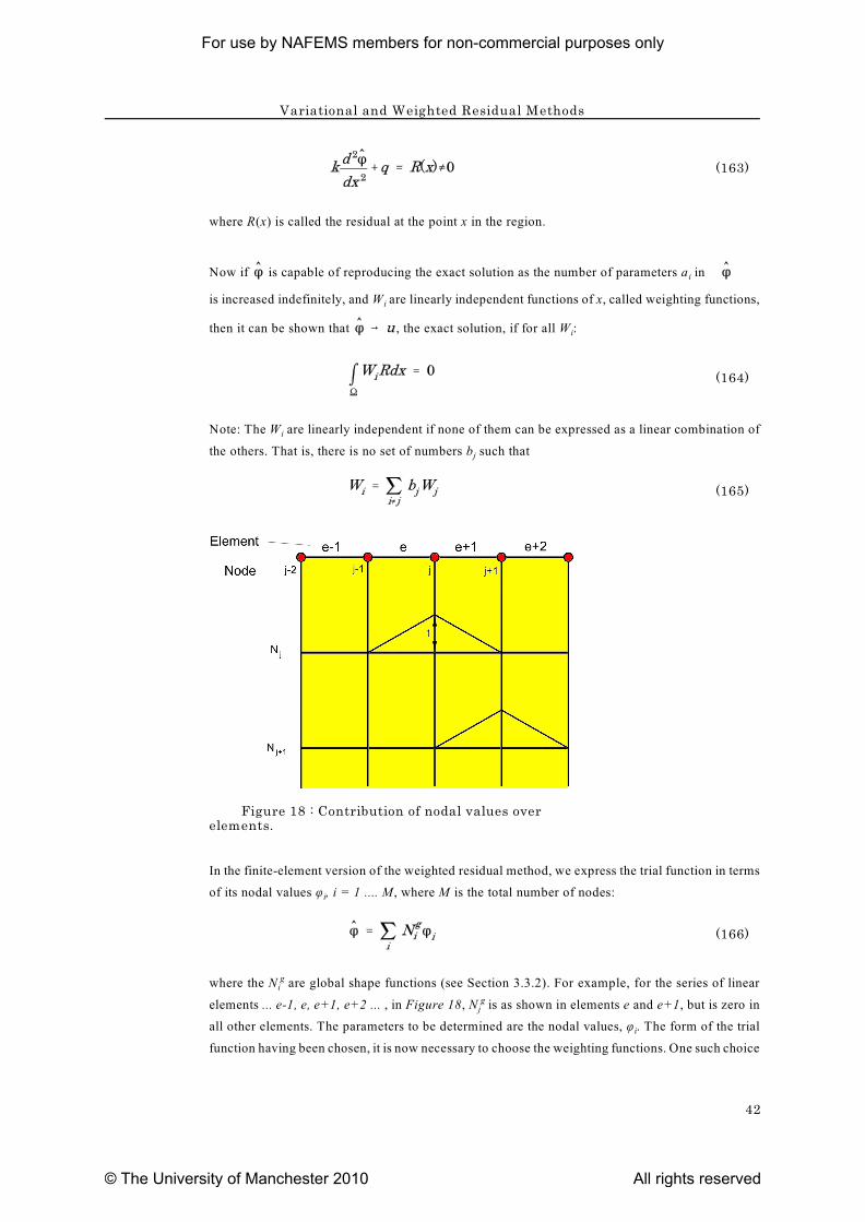
Figure 18 : Contribution of nodal values overelements.

(163)

where R(x) is called the residual at the point x in the region.

iNow if is capable of reproducing the exact solution as the number of parameters a in

iis increased indefinitely, and W are linearly independent functions of x, called weighting functions,

ithen it can be shown that , the exact solution, if for all W :

(164)

iNote: The W are linearly independent if none of them can be expressed as a linear combination of

jthe others. That is, there is no set of numbers b such that

(165)

In the finite-element version of the weighted residual method, we express the trial function in terms

iof its nodal values ö , i = 1 .... M, where M is the total number of nodes:

(166)

iwhere the N are global shape functions (see Section 3.3.2). For example, for the series of linearg

jelements ... e-1, e, e+1, e+2 ... , in Figure 18, N is as shown in elements e and e+1, but is zero ing

iall other elements. The parameters to be determined are the nodal values, ö . The form of the trial

function having been chosen, it is now necessary to choose the weighting functions. One such choice




43

is to make the weighting functions the same as the shape functions: this is the Galerkin method. The

weighted residual statement is then:

(167)

A problem here is that the method appears to fail with piece-wise linear shape functions, since

is everywhere zero (except at nodes where is discontinuous).

However, we may integrate by parts:

(168)

i áLooking at the second term on the right-hand side, we see that it is zero unless both N and Ng g

j j+1belong to the same finite element. For example, N and N both belong to element e+1. The firstg g

term on the right-hand side is also zero, apart from the two elements at the extremities of Ù. For the

first element:

(169)

Since

(170)

then

(171)

This can be written as

(172)

Again, since




44

(173)

this becomes

(174)

where the notation of the previous section has been used for . Similarly for the last element:

(175)

Hence

iágives the component K of the global stiffness matrix [K] andg

(176)

where

(177)

(178)

(179)

If we look at the j-th row of the matrix product [K] {ö}, the only non-zero terms are:g

(180)

(181)




45

(182)

jReverting to the shape functions within the individual elements, such as N , we see that these threee

non-zero terms can be expressed respectively as

(183)

j j-1which is an integral over element e, since N is zero for element numbers less than e and N is zerog g

for element numbers greater than e. Similarly the second term can be expressed as

(184)

and the third as,

(185)

Hence we can express the global stiffness matrix by assembling the element stiffness matrices [K] ,e

where

(186)

and á and â could each take on the values j-1 and j for the element e shown in Figure 18 and the

superfix has been removed from the element shape functions.

The result obtained by the Galerkin weighted residual method is exactly the same as that obtained

by the piece-wise application of the variational approach, using the Raleigh-Ritz method. The

stiffness matrices are symmetrical, which is advantageous in reducing the computation in solving the

system of simultaneous equations obtained.

Variational methods are extremely powerful in mathematical physics. They often provide an insight

into the basic principles governing the behaviour of a system. On the other hand, even if a variational

formulation of a certain problem is possible, the same results can be obtained by the Galerkin

weighted residual method and the latter can also be used when no variational formulation is available.

Although the Galerkin is the most commonly used of the weighted residual methods, it is possible

to use other weighting functions.




46

3.5 Extension to Two and Three Dimensions

The heat-conduction equation in two dimensions is:

(187)

for an isotropic medium. The weighted residual statement then becomes:

(188)

iwhere, as in the previous section, is a trial function containing M unknowns and W are M linearly

independent weighting functions, now of x and y and not of x alone. The integral is taken over the

area Ù in which the solution is sought.

The integral in equation (188) can be re-arranged by the use of Green's lemma, which is something

like a two-dimensional integration by parts:

(189)

and similarly:

(190)

x ywhere á and â are functions of x and y; n and n are the direction cosines of the outwards-pointing

normal to the closed curve Ã encompassing Ù. Applying Green's lemma to part of the integral in

equation (188) gives:

(191)

iin which á has been replaced by W and â by . So, with the sign changed, equation (188)

becomes:




47

(192)

The trial function is expressed in terms of the nodal values and piece-wise global shape functions:

(193)

so that the region Ù is divided up into finite elements within each of which is entirely determined

by the values of ö at the nodes lying on the boundary of the element or within the element. That is,

a node at the corner of an element will have a non-zero shape function only over the elements sharing

that corner; nodes on a boundary will have non-zero shape functions only over the two elements

meeting at the boundary, and internal nodes will have non-zero values only within the element to

which they belong.

In the weighted residual statement, equation (192), we now apply the Galerkin method and make the

i iweighting functions, W , the same as the shape functions, N :g

(194)

The left-hand side of this set of equations is the product of an M x M symmetrical matrix ([K] theg

global stiffness matrix) and the column vector of nodal values. The components of [K] are given by:g

(195)

npAs in the one-dimensional case, the K are made up of contributions from the various elementsg

n pwithin which both N and N are non-zero. For the element e, if n and p are nodes belonging to theg g

element and we omit the superfix e attached to the shape functions in the element, then the

npcomponent k of the element stiffness matrix is:e




48

(196)

and

(197)

or, in matrix form,

(198)

ewhere m is over the area of the element e and the integral over the boundary occurs only in the case

of elements with sides forming part of the boundary of Ù. The components of the element stiffness

matrices are assembled to form the global stiffness matrix. To do this, the components are placed in

ijthe global stiffness matrix in such a way as to multiply the correct ö : k therefore goes into the rowe

ilabelled i and the column labelled j. Similarly, f will be placed in row i. Quantities located in the

same position are simply added. The boundary conditions are inserted either in terms of specified

nodal values (Dirichlet) or specified values of and (Neumann conditions) in the

system of equations (194).

3.5.1 Three-noded element for thermal conduction

As in the linear triangular element for plane elasticity (Section 2.3), area shape functions are used to

áexpress in terms of the nodal values ö (Figure 13):

(199)

where, for example,

(200)

From this definition of the area shape functions, we have:




49

(201)

where Ä is the area of the triangle ijm. Differentiation then gives:

(202)

and

(203)

and similarly for the other shape functions. Hence, for example, equation (196) gives

(204)

and the element stiffness matrix becomes:

(205)

Turning now to the right-hand side of equation (197), let us assume that Q, and

are, or may be approximately represented by, values that are constant in the element. Then the first

term on the right-hand side is

(206)




50

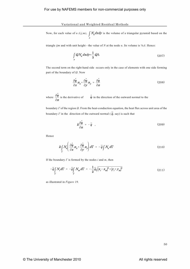
Now, for each value of á (i,j,m), is the volume of a triangular pyramid based on the

triangle ijm and with unit height - the value of N at the node á. Its volume is aÄ. Hence:

(207)

The second term on the right-hand side occurs only in the case of elements with one side forming

part of the boundary of Ù. Now

(208)

where is the derivative of in the direction of the outward normal to the

boundary Ã of the region Ù. From the heat-conduction equation, the heat flux across unit area of the

boundary Ã in the direction of the outward normal ( , say) is such that

(209)

Hence

(210)

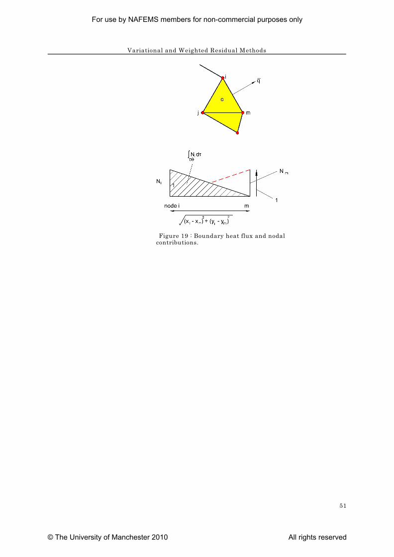
If the boundary Ã is formed by the nodes i and m, then

(211)

as illustrated in Figure 19.




51

Figure 19 : Boundary heat flux and nodalcontributions.



52

4 References

There are many textbooks on finite element analysis, but those that have been particularly used in preparing this

Introduction are:

Cheung, Y.K.,Yeo, M.F., A Practical Introduction to Finite Element Analysis, Pitman, 1979

Cook, R.D., Concepts and Applications of Finite Element Analysis (2nd edition), John Wiley and Sons, 1981

Huebner, K.H., Thornton, E.A., The Finite Element Method for Engineers (2nd edition), John Wiley and Sons, 1982

Zienkiewicz, O.C., The Finite Element Method,(4th edition), McGraw-Hill, 1991

Zienkiewicz, O.C., Morgan, K., Finite Elements and Approximation, John Wiley and Sons, 1982



53

Appendix 1

Review of Matrix Algebra

A Matrix

A matrix is a set of mxn quantities (its elements) arranged in the form of m rows and n columns. The

quantities in matrix may not all have the same dimensions: for example, some may be forces and

others may be moments. If m=1, the matrix is sometimes called a row matrix or a row vector and if

n=1, a column matrix or vector. This use of the term vector is not confined to the traditional vector

quantities, such as force or displacement.

The notation used in the present work is as follows: if m�1 and n�1, the matrix is denoted by a

symbol, usually a capital letter in bold type, contained in square brackets, [ ] , or by its elements

contained within square brackets. The elements are denoted by lower-case characters with

appropriate suffixes, the first standing for the row and the second for the column. For example, a

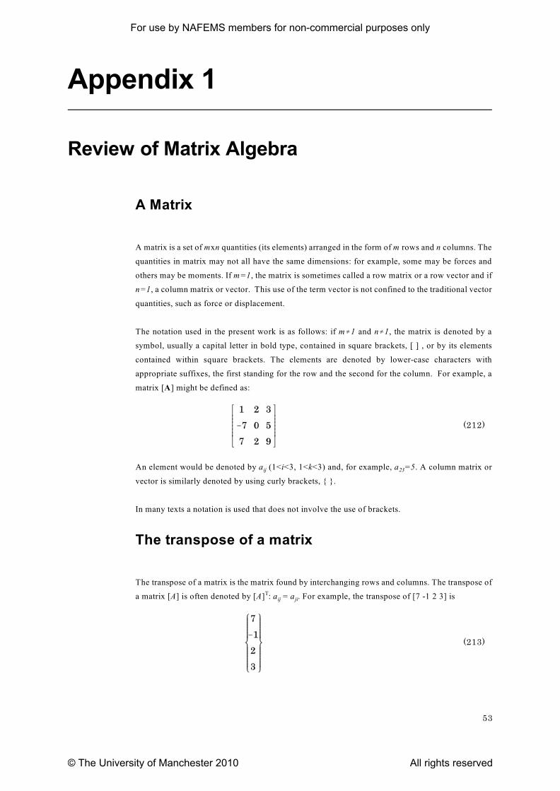
matrix [A] might be defined as:

(212)

ij 23An element would be denoted by a (1<i<3, 1<k<3) and, for example, a =5. A column matrix or

vector is similarly denoted by using curly brackets, { }.

In many texts a notation is used that does not involve the use of brackets.

The transpose of a matrix

The transpose of a matrix is the matrix found by interchanging rows and columns. The transpose of

ij jia matrix [A] is often denoted by [A] : a = a . For example, the transpose of [7 -1 2 3] is T

(213)



Appendix 1

54

To save space, a column matrix is sometimes shown as the transpose of a row matrix.

A square matrix

A square matrix has the same number of rows as columns i.e. m=n.

A Symmetrical Matrix

ij jiA symmetrical matrix is one in which corresponding off-diagonal terms are equal, that is a =a .

An anti-symmetric matrix

An anti-symmetric matrix is one in which the off-diagonal terms are of opposite sign but equal

absolute magnitude: the diagonal terms are zero. Both symmetrical and anti-symmetrical matrices

are, of course, square.

Equality, addition and subtraction of matrices

Only matrices which each have the same number of rows and columns may be equated, added or

subtracted.

Matrix equality

ij ijTwo matrices are equal if all their elements are equal: that is, [A]=[B] if a =b for all i and j.

Matrix addition

In matrix addition the values at each position ij within a matrix [A] are added to the value at position

ij ij ijij of a matrix [B] and the results placed in position of matrix [C]. i.e. [A]+[B]=[C]; c =a +b

Matrix subtraction

The value at position ij within a matrix [B] is subtracted from the value at position ij within a matrix

[A] and the result is placed in position ij in a matrix [C]. i.e.



Appendix 1

55

ij ij ij[A]-[B]=[C]; c =a -b

Matrix multiplication

Matrix multiplication is defined in the case of matrices that are conformable for multiplication. If

there is a product [A][B] of two matrices, then [A] must have the same number of columns as [B] has

rows. For example, if [A] is an (mxn) matrix and [B] is an (nxp) matrix, the product [A][B]=[C] will

be an (mxp) matrix with elements.

(214)

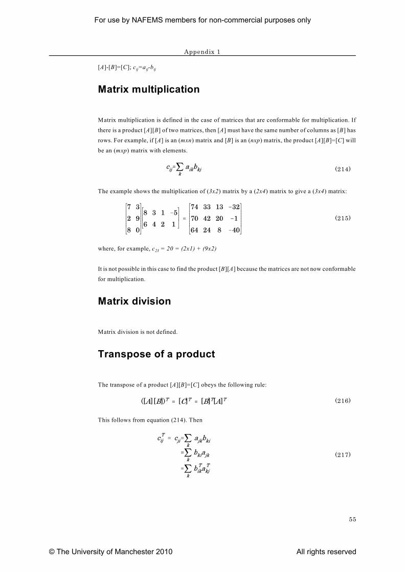
The example shows the multiplication of (3x2) matrix by a (2x4) matrix to give a (3x4) matrix:

(215)

23where, for example, c = 20 = (2x1) + (9x2)

It is not possible in this case to find the product [B][A] because the matrices are not now conformable

for multiplication.

Matrix division

Matrix division is not defined.

Transpose of a product

The transpose of a product [A][B]=[C] obeys the following rule:

(216)

This follows from equation (214). Then

(217)



Appendix 1

56

or

(218)

Inverse of a square matrix

The inverse of a square matrix [A] is denoted by [A] , and it is such that-1

(219)

where [I] is the unit matrix or the identity matrix, which has all its diagonal elements equal to 1 and

all remaining elements equal to zero. Multiplication of a matrix by the appropriate unit matrix (that

is, with the correct number of rows and, of course, the same number of columns) leaves the elements

of the matrix unaltered. The expression for the inverse of a matrix is given below. An orthogonal

matrix is a square matrix whose inverse is equal to its transpose. For example, if and axes are

obtained by rotation through an angle è anticlockwise with respect to the x and y axes, then the two

sets of axes are related by

(220)

or

(221)

It is readily shown that [R][R] =[I] so that [R] =[R] , or [R] is orthogonal.T T -1

Determiant of a square matrix

The determinant of a square matrix is found by multiplying out its elements: it is a number and is

denoted by det A or |A|. For example:



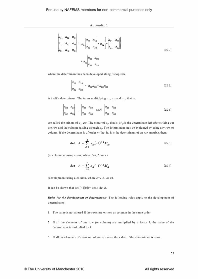
Appendix 1

57

(222)

where the determinant has been developed along its top row.

(223)

11 12 13is itself a determinant. The terms multiplying a , a and a , that is,

(224)

11 ij ijare called the minors of a etc. The minor of a , that is, M , is the determinant left after striking out

ijthe row and the column passing through a . The determinant may be evaluated by using any row or

column: if the determinant is of order n (that is, it is the determinant of an nxn matrix), then:

(225)

(development using a row, where i=1,2...or n)

(226)

(development using a column, where k=1,2...or n).

It can be shown that det([A][B])= det A det B.

Rules for the development of determinants. The following rules apply to the development of

determinants:

1. The value is not altered if the rows are written as columns in the same order.

2. If all the elements of one row (or column) are multiplied by a factor k, the value of the

determinant is multiplied by k.

3. If all the elements of a row or column are zero, the value of the determinant is zero.



Appendix 1

58

4. If any two rows or columns are interchanged, the value of the determinant is multiplied by -1.

5. If the corresponding elements of two rows or two columns are proportional, the value of the

determinant is zero.

6. The value of a determinant is unchanged if the elements of a row (or column) are changed by

adding to them any constant multiple of the corresponding elements of any other row (or

column).

Expression for the inverse of a square matrix

The minor of an element of a square matrix has been defined above. The cofactor of an element is

equal to the minor multiplied by the sign in front of it in the development of the determinant. The

ij ijcofactor of a , denoted by A , is then

(227)

If each element in the matrix is replaced by its cofactor and the transpose of the resulting matrix is

taken, that matrix is called the adjoint of [A], [adj A]. It can be shown that:

(228)

Clearly [A] is not defined if det A=0. The matrix is then said to be singular.-1



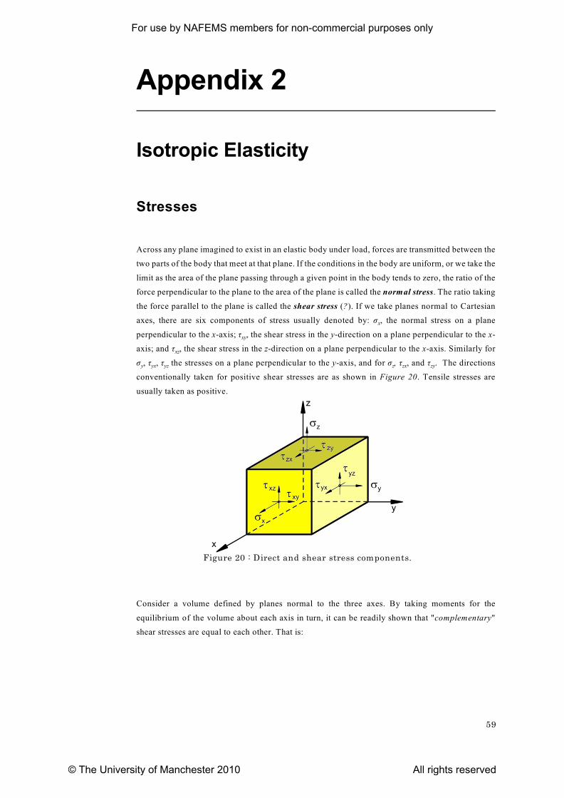
59

Figure 20 : Direct and shear stress components.

Appendix 2

Isotropic Elasticity

Stresses

Across any plane imagined to exist in an elastic body under load, forces are transmitted between the

two parts of the body that meet at that plane. If the conditions in the body are uniform, or we take the

limit as the area of the plane passing through a given point in the body tends to zero, the ratio of the

force perpendicular to the plane to the area of the plane is called the normal stress. The ratio taking

the force parallel to the plane is called the shear stress (?). If we take planes normal to Cartesian

xaxes, there are six components of stress usually denoted by: ó , the normal stress on a plane

xyperpendicular to the x-axis; ô , the shear stress in the y-direction on a plane perpendicular to the x-

xzaxis; and ô , the shear stress in the z-direction on a plane perpendicular to the x-axis. Similarly for

y yx yz z zx zyó , ô , ô the stresses on a plane perpendicular to the y-axis, and for ó , ô , and ô . The directions

conventionally taken for positive shear stresses are as shown in Figure 20. Tensile stresses are

usually taken as positive.

Consider a volume defined by planes normal to the three axes. By taking moments for the

equilibrium of the volume about each axis in turn, it can be readily shown that "complementary"

shear stresses are equal to each other. That is:



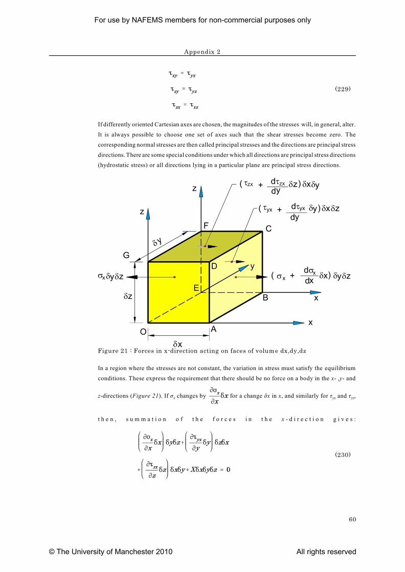
Appendix 2

60

(229)

If differently oriented Cartesian axes are chosen, the magnitudes of the stresses will, in general, alter.

It is always possible to choose one set of axes such that the shear stresses become zero. The

corresponding normal stresses are then called principal stresses and the directions are principal stress

directions. There are some special conditions under which all directions are principal stress directions

(hydrostatic stress) or all directions lying in a particular plane are principal stress directions.

In a region where the stresses are not constant, the variation in stress must satisfy the equilibrium

conditions. These express the requirement that there should be no force on a body in the x- ,y- and

x yx zxz-directions (Figure 21). If ó changes by for a change äx in x, and similarly for ô and ô ,

t h e n , s u m m a t i o n o f t h e f o r c e s i n t h e x - d i r e c t i o n g i v e s :

(230)

Figure 21 : Forces in x-direction acting on faces of volume dx,dy,dz



Appendix 2

61

or

(231)

and similarly

(232)

and

(233)

where X, Y and Z are body forces, for example, gravity forces (per unit volume) acting respectively

in the x-, y- and z-directions.

Relationship between displacement and strain

The strains used in the theory of elasticity are "infinitesimal" or vanishingly small quantities. Figure

22 shows a region before, ijkl, and after, i'j'k'l', deformation. The strain in the x-direction is defined

as the change in length of a fibre parallel to the x-axis, divided by its original length. For the line ij,

then

(234)

Similarly

(235)

xyThe engineering shear strain, â , is defined to be the change in the right-angle lij: that is, (Figure

22).

(236)



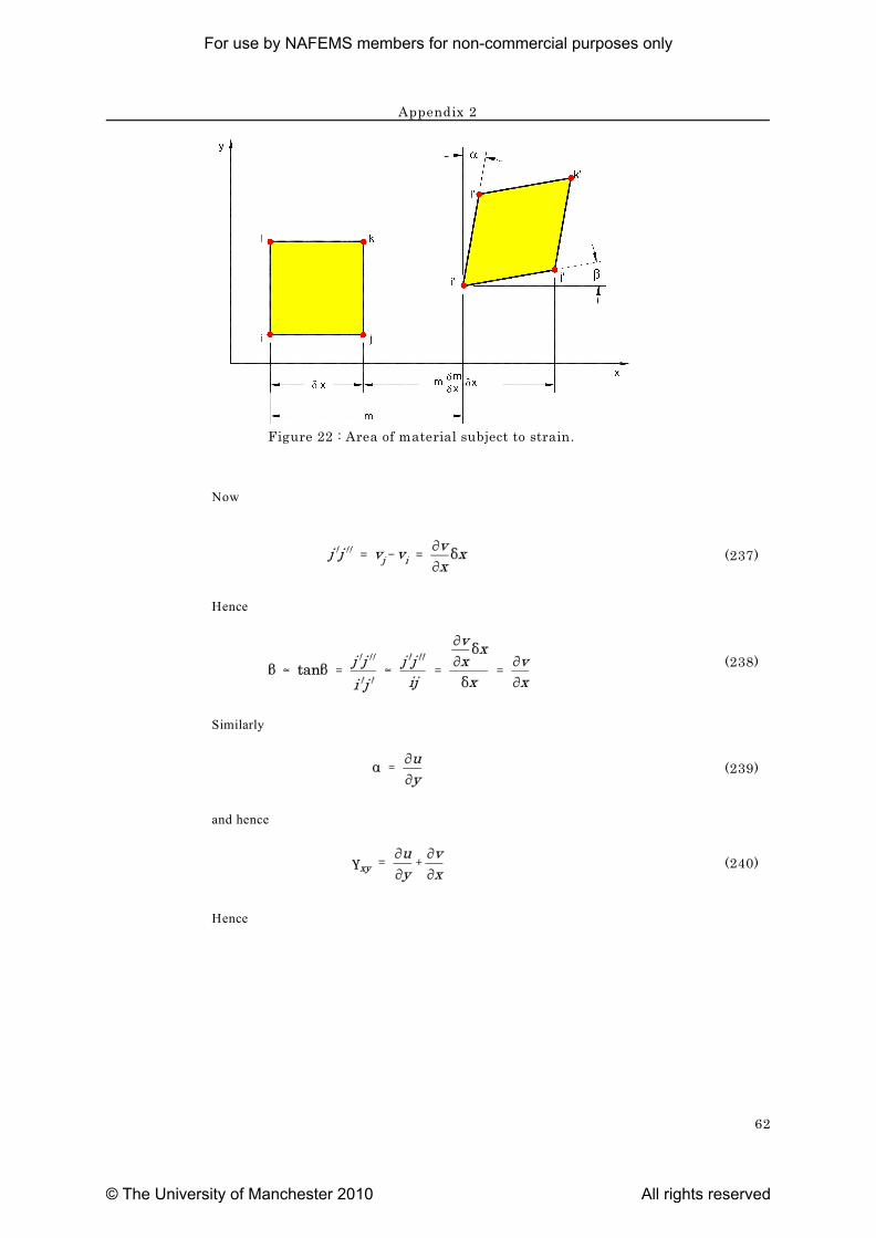
Appendix 2

62

Figure 22 : Area of material subject to strain.

Now

(237)

Hence

(238)

Similarly

(239)

and hence

(240)

Hence



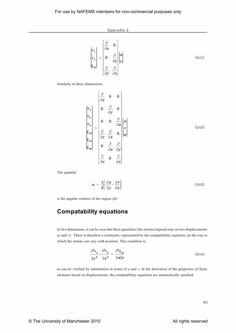
Appendix 2

63

(241)

Similarly in three dimensions:

(242)

The quantity

(243)

is the angular rotation of the region ijkl.

Compatability equations

In two dimensions, it can be seen that three quantities (the strains) depend only on two displacements

(u and v). There is therefore a constraint, represented by the compatability equation, on the way in

which the strains can vary with position. This condition is:

(244)

as can be verified by substitution in terms of u and v. In the derivation of the properties of finite

elements based on displacements, the compatability equations are automatically satisfied.



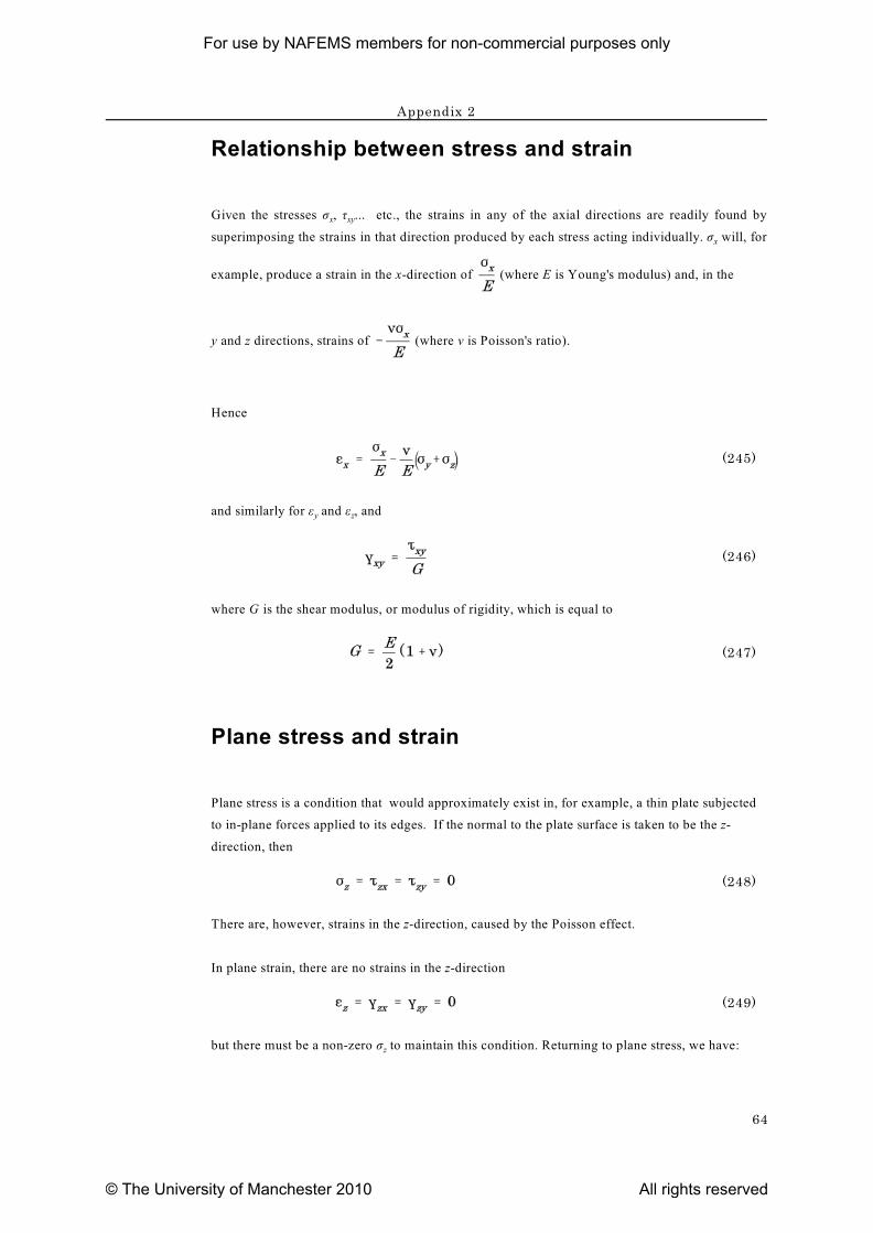
Appendix 2

64

Relationship between stress and strain

x xyGiven the stresses ó , ô ... etc., the strains in any of the axial directions are readily found by

xsuperimposing the strains in that direction produced by each stress acting individually. ó will, for

example, produce a strain in the x-direction of (where E is Young's modulus) and, in the

y and z directions, strains of (where í is Poisson's ratio).

Hence

(245)

y zand similarly for å and å , and

(246)

where G is the shear modulus, or modulus of rigidity, which is equal to

(247)

Plane stress and strain

Plane stress is a condition that would approximately exist in, for example, a thin plate subjected

to in-plane forces applied to its edges. If the normal to the plate surface is taken to be the z-

direction, then

(248)

There are, however, strains in the z-direction, caused by the Poisson effect.

In plane strain, there are no strains in the z-direction

(249)

zbut there must be a non-zero ó to maintain this condition. Returning to plane stress, we have:



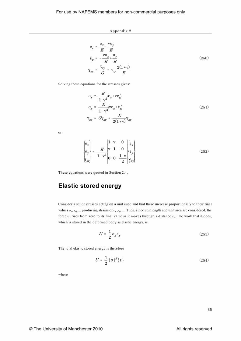
Appendix 2

65

(250)

Solving these equations for the stresses gives:

(251)

or

(252)

These equations were quoted in Section 2.4.

Elastic stored energy

Consider a set of stresses acting on a unit cube and that these increase proportionally to their final

x xy x, xyvalues ó , ô .... producing strains of å ã .... Then, since unit length and unit area are considered, the

x xforce ó rises from zero to its final value as it moves through a distance å . The work that it does,

which is stored in the deformed body as elastic energy, is

(253)

The total elastic stored energy is therefore

(254)

where



Appendix 2

66

(255)

In considering virtual work, one must remember that the stresses remain constant as the virtual strains

are produced.

Hence the virtual work done is ,

where are the virtual strains.

Symmetry of the elasticity matrix

The elasticity matrix, [D], relates the stresses to the strains for specific conditions of loading. To

show that [D] must be symmetrical, we note that

(256)

and similarly for the other stresses.

Hence, for example,

(257)

etc. But, if U is the elastic stored energy per unit volume,

(258)

and so

(259)

Similarly,

(260)



Appendix 2

67

and

(261)

12 21Hence D = D . This result holds similarly for the other off-diagonal terms and [D] must therefore

be symmetrical. This result holds for both isotropic and anisotropic behaviour.



68

Appendix 3

Shape Functions

Displacement functions

The variable to be evaluated within an element can be expressed explicitly in terms of the nodal

values by the use of shape functions (Section 2.3). An alternative procedure is to express the

variable as a polynomial (or some other function) with coefficients to be determined from the nodal

values. For example, for a three-noded triangular element, the variable ö could be expressed as:

(262)

Since this expression must also hold for the nodal values:

(263)

or

(264)

so that

(265)

In this way,

(266)

Hence



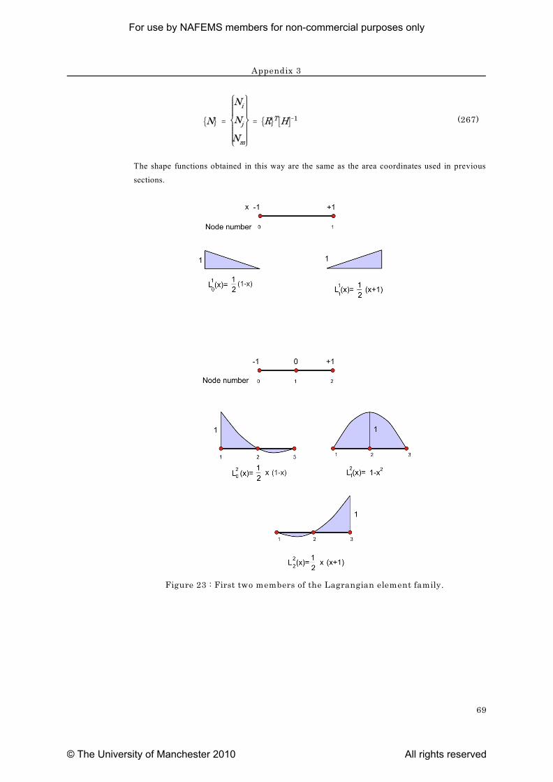
Appendix 3

69

Figure 23 : First two members of the Lagrangian element family.

(267)

The shape functions obtained in this way are the same as the area coordinates used in previous

sections.



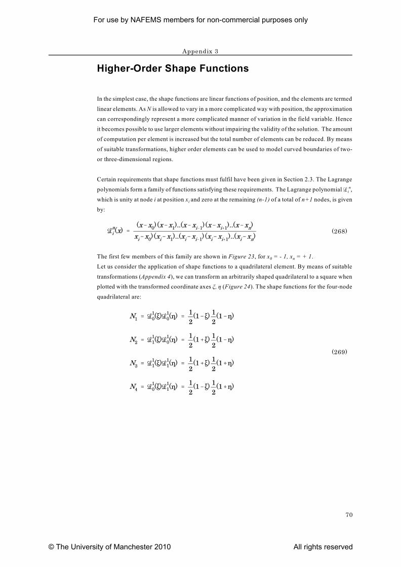
Appendix 3

70

Higher-Order Shape Functions

In the simplest case, the shape functions are linear functions of position, and the elements are termed

linear elements. As N is allowed to vary in a more complicated way with position, the approximation

can correspondingly represent a more complicated manner of variation in the field variable. Hence

it becomes possible to use larger elements without impairing the validity of the solution. The amount

of computation per element is increased but the total number of elements can be reduced. By means

of suitable transformations, higher order elements can be used to model curved boundaries of two-

or three-dimensional regions.

Certain requirements that shape functions must fulfil have been given in Section 2.3. The Lagrange

ipolynomials form a family of functions satisfying these requirements. The Lagrange polynomial � ,n

iwhich is unity at node i at position x and zero at the remaining (n-1) of a total of n+1 nodes, is given

by:

(268)

0 nThe first few members of this family are shown in Figure 23, for x = - 1, x = + 1.

Let us consider the application of shape functions to a quadrilateral element. By means of suitable

transformations (Appendix 4), we can transform an arbitrarily shaped quadrilateral to a square when

plotted with the transformed coordinate axes î, ç (Figure 24). The shape functions for the four-node

quadrilateral are:

(269)



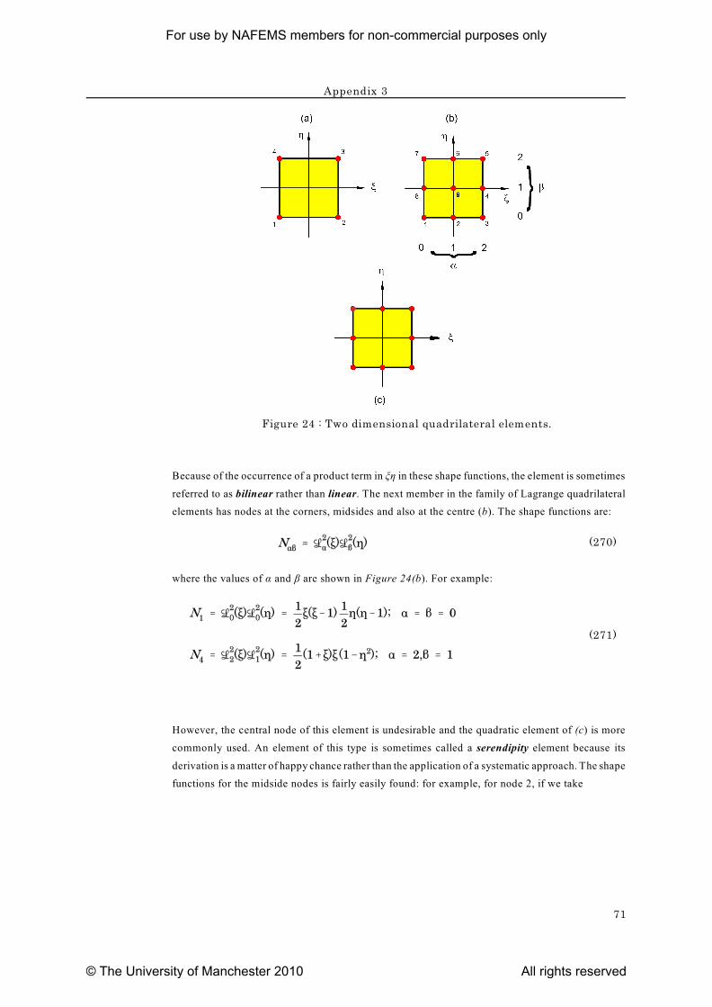
Appendix 3

71

Figure 24 : Two dimensional quadrilateral elements.

Because of the occurrence of a product term in îç in these shape functions, the element is sometimes

referred to as bilinear rather than linear. The next member in the family of Lagrange quadrilateral

elements has nodes at the corners, midsides and also at the centre (b). The shape functions are:

(270)

where the values of á and â are shown in Figure 24(b). For example:

(271)

However, the central node of this element is undesirable and the quadratic element of (c) is more

commonly used. An element of this type is sometimes called a serendipity element because its

derivation is a matter of happy chance rather than the application of a systematic approach. The shape

functions for the midside nodes is fairly easily found: for example, for node 2, if we take



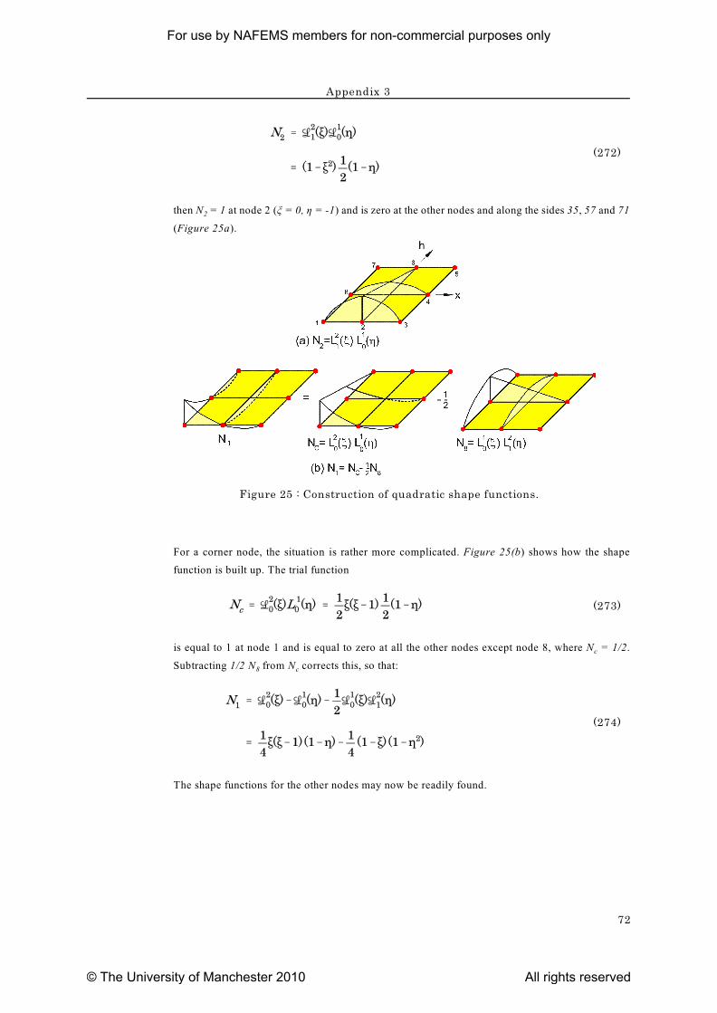
Appendix 3

72

Figure 25 : Construction of quadratic shape functions.

(272)

2then N = 1 at node 2 (î = 0, ç = -1) and is zero at the other nodes and along the sides 35, 57 and 71

(Figure 25a).

For a corner node, the situation is rather more complicated. Figure 25(b) shows how the shape

function is built up. The trial function

(273)

cis equal to 1 at node 1 and is equal to zero at all the other nodes except node 8, where N = 1/2.

8 cSubtracting 1/2 N from N corrects this, so that:

(274)

The shape functions for the other nodes may now be readily found.



Appendix 3

73

Continuity of first derivatives

The shape functions referred to above provide C continuity between elements: that is, the fieldo

variable is continuous between elements but its derivatives are not. In structural analysis, continuity

of the first derivative (C continuity) is required when rotation, in addition to displacement, is a nodal1

degree of freedom. Examples occur in the case of beam elements and shell elements.

Functions of this type may be expressed in terms of Hermitian polynomials.

If, for a straight two-noded beam element extending from x = -1 to x = +1, we express w in terms

1 2 1 2of the displacements, w and w , and the rotations, ö and ö , at the ends of the beam element, then:

(275)

and

(276)

1Since the nodal values are prescribed, it follows for N that

(277)

2and for N :

(278)

3 4and similarly for N and N .

The simplest polynomials satisfying these conditions are cubic. By solving for the coefficients, it is

readily found that:



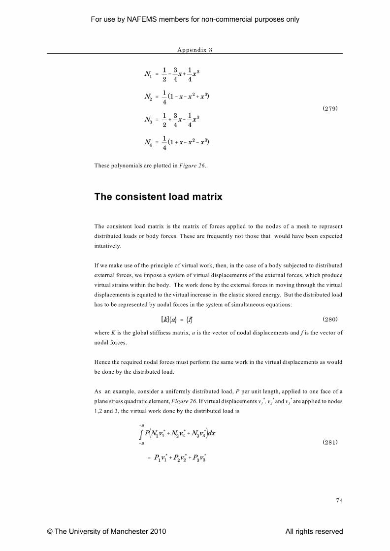
Appendix 3

74

(279)

These polynomials are plotted in Figure 26.

The consistent load matrix

The consistent load matrix is the matrix of forces applied to the nodes of a mesh to represent

distributed loads or body forces. These are frequently not those that would have been expected

intuitively.

If we make use of the principle of virtual work, then, in the case of a body subjected to distributed

external forces, we impose a system of virtual displacements of the external forces, which produce

virtual strains within the body. The work done by the external forces in moving through the virtual

displacements is equated to the virtual increase in the elastic stored energy. But the distributed load

has to be represented by nodal forces in the system of simultaneous equations:

(280)

where K is the global stiffness matrix, a is the vector of nodal displacements and f is the vector of

nodal forces.

Hence the required nodal forces must perform the same work in the virtual displacements as would

be done by the distributed load.

As an example, consider a uniformly distributed load, P per unit length, applied to one face of a

1 2 3plane stress quadratic element, Figure 26. If virtual displacements v , v and v are applied to nodes* * *

1,2 and 3, the virtual work done by the distributed load is

(281)



Appendix 3

75

Figure 26 : Distributed and equivalent loading.

1 2 3where P , P and P are the required nodal forces.

Since the v 's are arbitrary:*

(282)

In terms of x, the shape functions determining the displacement of points along the boundary 123 of

the element are

(283)

(284)

and



Appendix 3

76

(285)

Performing the required integration gives

(286)

and

(287)

where 2Pa is the total load applied to the boundary 123.

Other forms of loading, for example, a distributed load rising uniformly from zero at node 1 to node

2, are found by expressing P as an appropriate function of x. Complicated distributions cannot,

however, be realistically modelled without refinement of the mesh. Body forces require the

integration to be performed over the volume of the element. The representation of distributed loads

by nodal forces that are statically equivalent to the applied loads but differ from the consistent loads

will adversely affect the finite-element analysis near to the region where the loads are applied, but

not in regions that are more remote.



77

Appendix 4

Rotation of axes & Isoparametricelements.

Rotation of axes

It is sometimes convenient to use local Cartesian axes, differently oriented from the global Cartesian

axes, in delineating some elements in a structure. It then becomes necessary to convert the properties

obtained in the local axial system to those in the global system. In this Appendix, we shall deal with

the effect of the rotation of axes on the components of stress, strain and the element stiffness matrix.

We shall consider old axes x, y and z and new axes and .

11In addition, we shall denote the direction cosine between the old x axis and the new x axis, a , that

23between the old y axis and the new z axis, a , and so on. Then the component of a vector F in the

new direction is found by taking the resolved part of each component in the old axes in the new

direction and is given by:

(288)

or, for all the new components:

(289)

To find how the components of the stress change, consider the equilibrium of the volume shown in

1 2 3Figure 27. The oblique plane of unit area has a normal with direction cosines n , n and n .



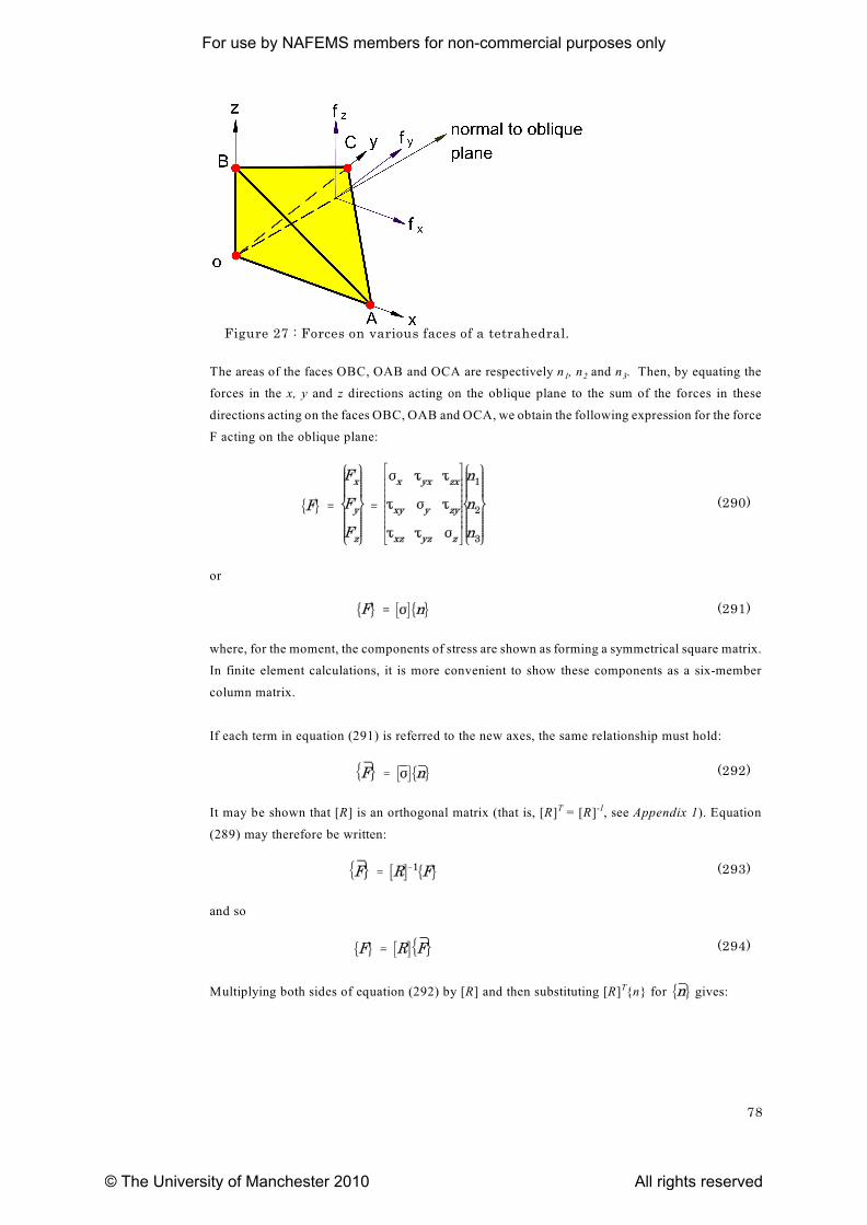
78

Figure 27 : Forces on various faces of a tetrahedral.

1 2 3The areas of the faces OBC, OAB and OCA are respectively n , n and n . Then, by equating the

forces in the x, y and z directions acting on the oblique plane to the sum of the forces in these

directions acting on the faces OBC, OAB and OCA, we obtain the following expression for the force

F acting on the oblique plane:

(290)

or

(291)

where, for the moment, the components of stress are shown as forming a symmetrical square matrix.

In finite element calculations, it is more convenient to show these components as a six-member

column matrix.

If each term in equation (291) is referred to the new axes, the same relationship must hold:

(292)

It may be shown that [R] is an orthogonal matrix (that is, [R] = [R] , see Appendix 1). EquationT -1

(289) may therefore be written:

(293)

and so

(294)

Multiplying both sides of equation (292) by [R] and then substituting [R] {n} for gives:T



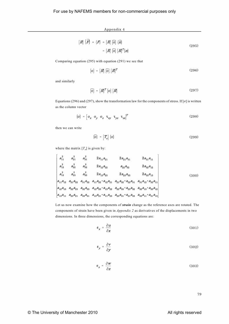
Appendix 4

79

(295)

Comparing equation (295) with equation (291) we see that

(296)

and similarly

(297)

Equations (296) and (297), show the transformation law for the components of stress. If [ó] is written

as the column vector

(298)

then we can write

(299)

ówhere the matrix [T ] is given by:

(300)

Let us now examine how the components of strain change as the reference axes are rotated. The

components of strain have been given in Appendix 2 as derivatives of the displacements in two

dimensions. In three dimensions, the corresponding equations are:

(301)

(302)

(303)



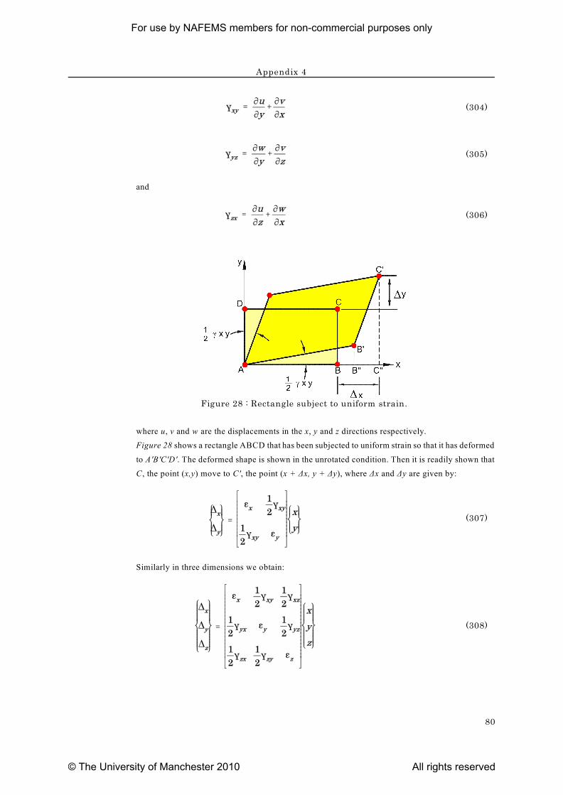
Appendix 4

80

Figure 28 : Rectangle subject to uniform strain.

(304)

(305)

and

(306)

where u, v and w are the displacements in the x, y and z directions respectively.

Figure 28 shows a rectangle ABCD that has been subjected to uniform strain so that it has deformed

to A'B'C'D'. The deformed shape is shown in the unrotated condition. Then it is readily shown that

C, the point (x,y) move to C', the point (x + Äx, y + Äy), where Äx and Äy are given by:

(307)

Similarly in three dimensions we obtain:

(308)



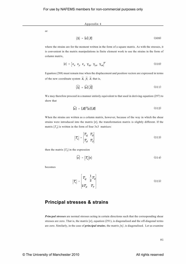
Appendix 4

81

or

(309)

where the strains are for the moment written in the form of a square matrix. As with the stresses, it

is convenient in the matrix manipulations in finite element work to use the strains in the form of

column matrix,

(310)

Equation (288) must remain true when the displacement and position vectors are expressed in terms

of the new coordinate system , that is,

(311)

We may therefore proceed in a manner entirely equivalent to that used in deriving equation (297) to

show that

(312)

When the strains are written as a column matrix, however, because of the way in which the shear

strains were introduced into the matrix [g], the transformation matrix is slightly different. If the

ömatrix [T ] is written in the form of four 3x3 matrices:

(313)

gthen the matrix [T ] in the expression

(314)

becomes

(315)

Principal stresses & strains

Princpal stresses are normal stresses acting in certain directions such that the corresponding shear

stresses are zero. That is, the matrix [ó], equation (291), is diagonalised and the off-diagonal terms

are zero. Similarly, in the case of principal strains, the matrix [g] , is diagonalised. Let us examine



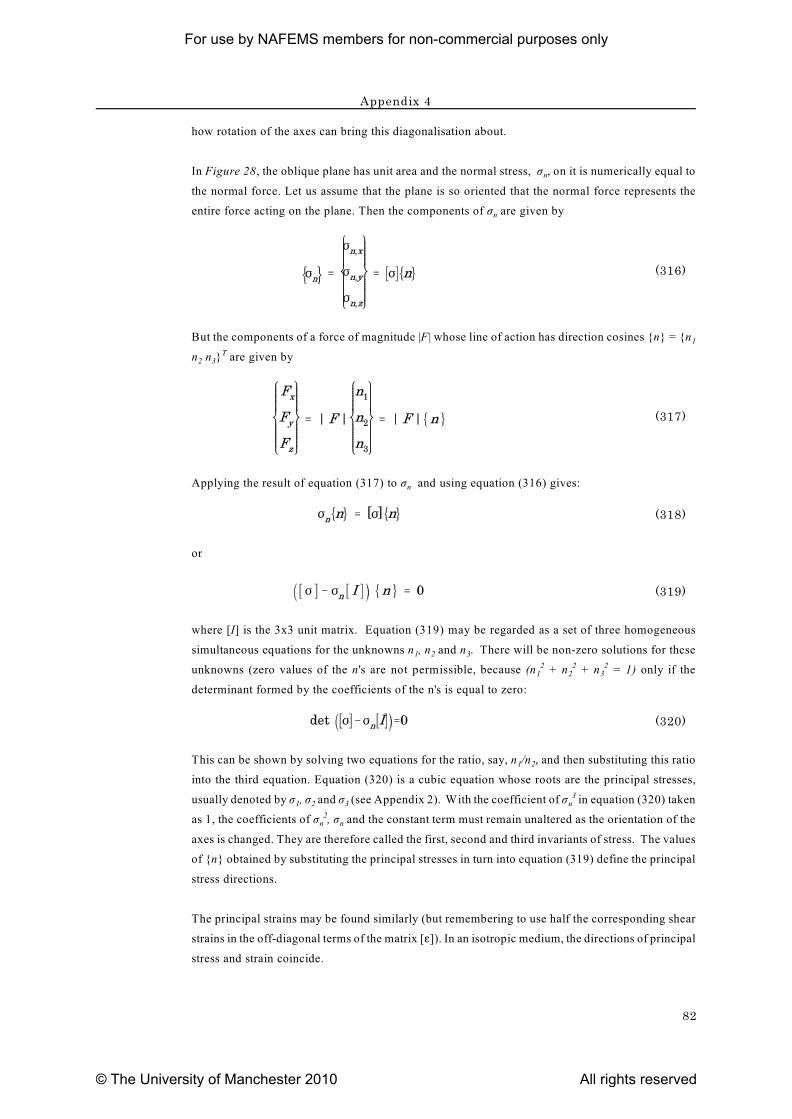
Appendix 4

82

how rotation of the axes can bring this diagonalisation about.

nIn Figure 28, the oblique plane has unit area and the normal stress, ó , on it is numerically equal to

the normal force. Let us assume that the plane is so oriented that the normal force represents the

nentire force acting on the plane. Then the components of ó are given by

(316)

1But the components of a force of magnitude |F| whose line of action has direction cosines {n} = {n

2 3n n } are given byT

(317)

nApplying the result of equation (317) to ó and using equation (316) gives:

(318)

or

(319)

where [I] is the 3x3 unit matrix. Equation (319) may be regarded as a set of three homogeneous

1 2 3simultaneous equations for the unknowns n , n and n . There will be non-zero solutions for these

1 2 3unknowns (zero values of the n's are not permissible, because (n + n + n = 1) only if the2 2 2

determinant formed by the coefficients of the n's is equal to zero:

(320)

1 2This can be shown by solving two equations for the ratio, say, n /n , and then substituting this ratio

into the third equation. Equation (320) is a cubic equation whose roots are the principal stresses,

1 2 3 nusually denoted by ó , ó and ó (see Appendix 2). With the coefficient of ó in equation (320) taken3

n nas 1, the coefficients of ó , ó and the constant term must remain unaltered as the orientation of the2

axes is changed. They are therefore called the first, second and third invariants of stress. The values

of {n} obtained by substituting the principal stresses in turn into equation (319) define the principal

stress directions.

The principal strains may be found similarly (but remembering to use half the corresponding shear

strains in the off-diagonal terms of the matrix [g]). In an isotropic medium, the directions of principal

stress and strain coincide.



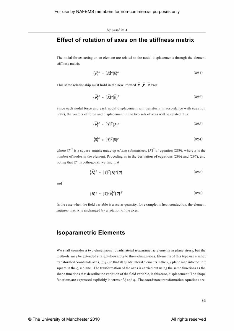
Appendix 4

83

Effect of rotation of axes on the stiffness matrix

The nodal forces acting on an element are related to the nodal displacements through the element

stiffness matrix

(321)

This same relationship must hold in the new, rotated axes:

(322)

Since each nodal force and each nodal displacement will transform in accordance with equation

(289), the vectors of force and displacement in the two sets of axes will be related thus:

(323)

(324)

where [T] is a square matrix made up of nxn submatrices, [R] of equation (289), where n is theT T

number of nodes in the element. Proceding as in the derivation of equations (296) and (297), and

noting that [T] is orthogonal, we find that

(325)

and

(326)

In the case when the field variable is a scalar quantity, for example, in heat conduction, the element

stiffness matrix is unchanged by a rotation of the axes.

Isoparametric Elements

We shall consider a two-dimensional quadrilateral isoparametric elements in plane stress, but the

methods may be extended straight-forwardly to three-dimensions. Elements of this type use a set of

transformed coordinate axes, (î,ç), so that all quadrilateral elements in the x, y plane map into the unit

square in the î, ç plane. The tranformation of the axes is carried out using the same functions as the

shape functions that describe the variation of the field variable, in this case, displacement. The shape

functions are expressed explicitly in terms of î and ç. The coordinate transformation equations are:



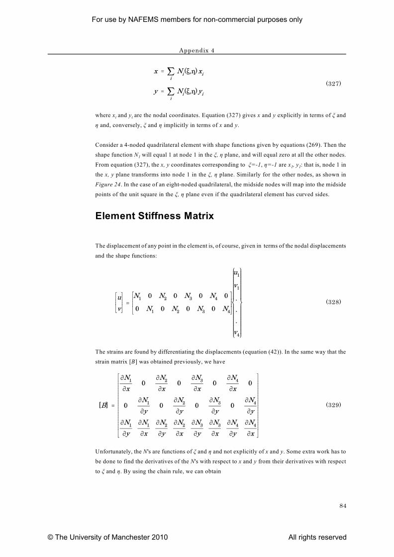
Appendix 4

84

(327)

i iwhere x and y are the nodal coordinates. Equation (327) gives x and y explicitly in terms of î and

ç and, conversely, î and ç implicitly in terms of x and y.

Consider a 4-noded quadrilateral element with shape functions given by equations (269). Then the

1shape function N will equal 1 at node 1 in the î, ç plane, and will equal zero at all the other nodes.

1 1From equation (327), the x, y coordinates corresponding to î=-1, ç=-1 are x , y : that is, node 1 in

the x, y plane transforms into node 1 in the î, ç plane. Similarly for the other nodes, as shown in

Figure 24. In the case of an eight-noded quadrilateral, the midside nodes will map into the midside

points of the unit square in the î, ç plane even if the quadrilateral element has curved sides.

Element Stiffness Matrix

The displacement of any point in the element is, of course, given in terms of the nodal displacements

and the shape functions:

(328)

The strains are found by differentiating the displacements (equation (42)). In the same way that the

strain matrix [B] was obtained previously, we have

(329)

Unfortunately, the N's are functions of î and ç and not explicitly of x and y. Some extra work has to

be done to find the derivatives of the N's with respect to x and y from their derivatives with respect

to î and ç. By using the chain rule, we can obtain



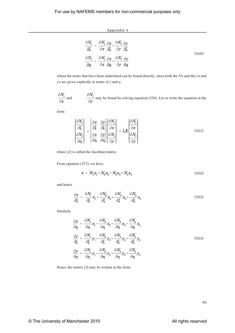
Appendix 4

85

(330)

where the terms that have been underlined can be found directly, since both the N's and the x's and

y's are given explicitly in terms of î and ç.

and may be found by solving equation (330). Let us write the equation in the

form:

(331)

where [J] is called the Jacobian matrix.

From equation (327), we have

(332)

and hence

(333)

Similarly

(334)

Hence the matrix [J] may be written in the form:



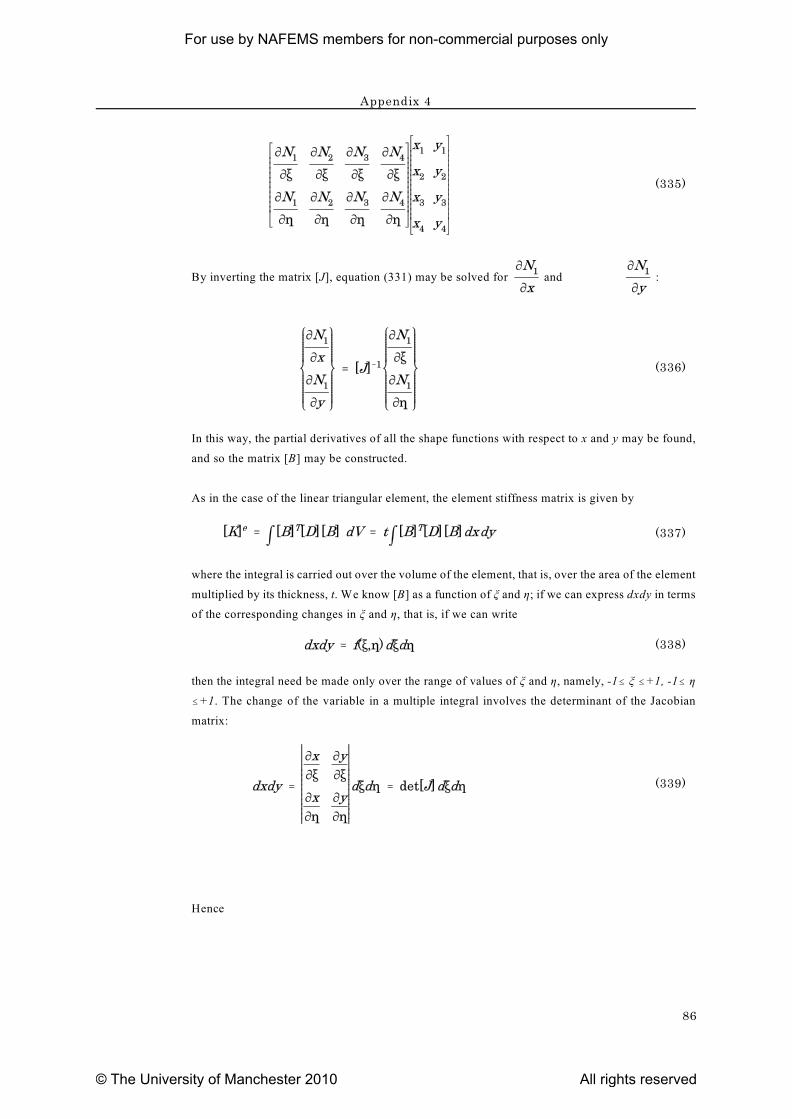
Appendix 4

86

(335)

By inverting the matrix [J], equation (331) may be solved for and :

(336)

In this way, the partial derivatives of all the shape functions with respect to x and y may be found,

and so the matrix [B] may be constructed.

As in the case of the linear triangular element, the element stiffness matrix is given by

(337)

where the integral is carried out over the volume of the element, that is, over the area of the element

multiplied by its thickness, t. We know [B] as a function of î and ç; if we can express dxdy in terms

of the corresponding changes in î and ç, that is, if we can write

(338)

then the integral need be made only over the range of values of î and ç, namely, -1# î #+1, -1# ç

#+1. The change of the variable in a multiple integral involves the determinant of the Jacobian

matrix:

(339)

Hence



Appendix 4

87

(340)

The integral has to be evaluated by numerical methods.



introduction to finite element analysis - nafems · pdf fileiv acknowledgements this manual is...

Documents