Introduction to Graphing Using MATLAB

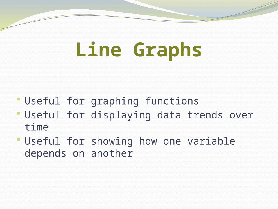
Line Graphs

Useful for graphing functions Useful for displaying data trends over time Useful for showing how one variable depends on

another

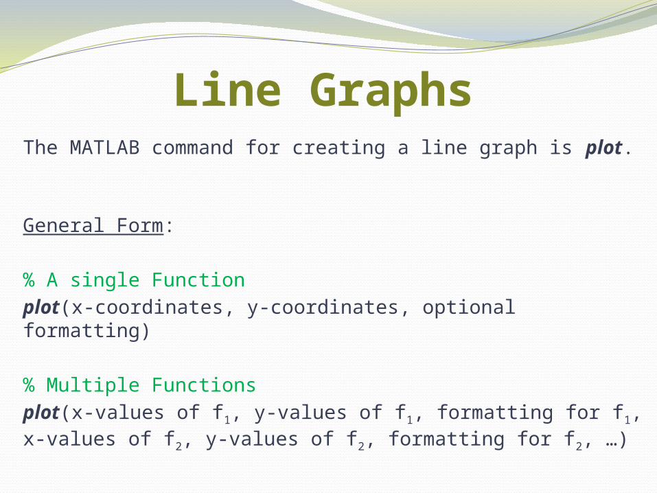
Line GraphsThe MATLAB command for creating a line graph is plot.

General Form:

% A single Function

plot(x-coordinates, y-coordinates, optional formatting)

% Multiple Functions

plot(x-values of f1, y-values of f1, formatting for f1, x-values of f2, y-values of f2, formatting for f2, …)

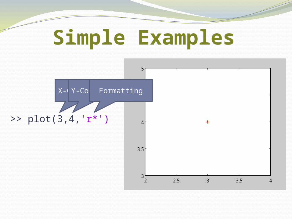
Simple Examples

>> plot(3,4,'r*')

2 2.5 3 3.5 43

3.5

4

4.5

5

X-CoordinatesY-CoordinatesFormatting

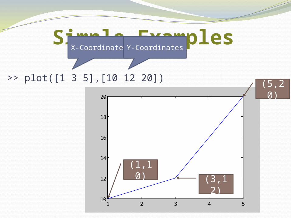
Simple Examples

>> plot([1 3 5],[10 12 20])

1 2 3 4 510

12

14

16

18

20

X-Coordinates Y-Coordinates

(1,10)

(3,12)

(5,20)

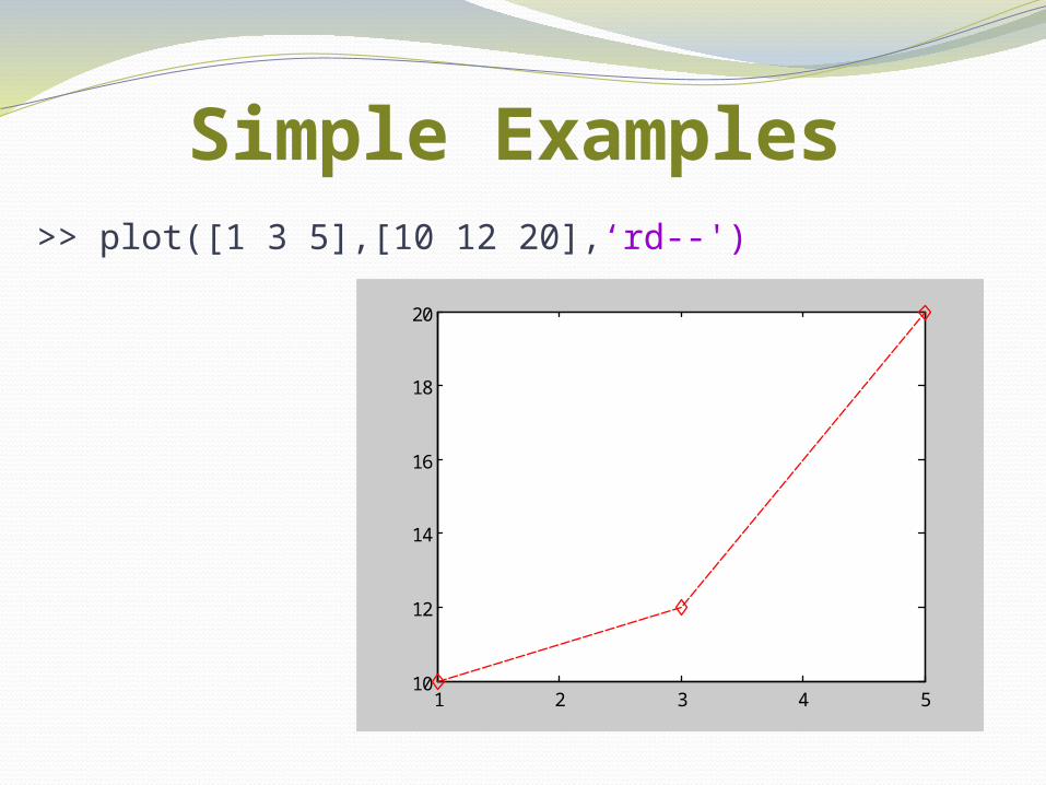
Simple Examples>> plot([1 3 5],[10 12 20],‘rd--')

1 2 3 4 510

12

14

16

18

20

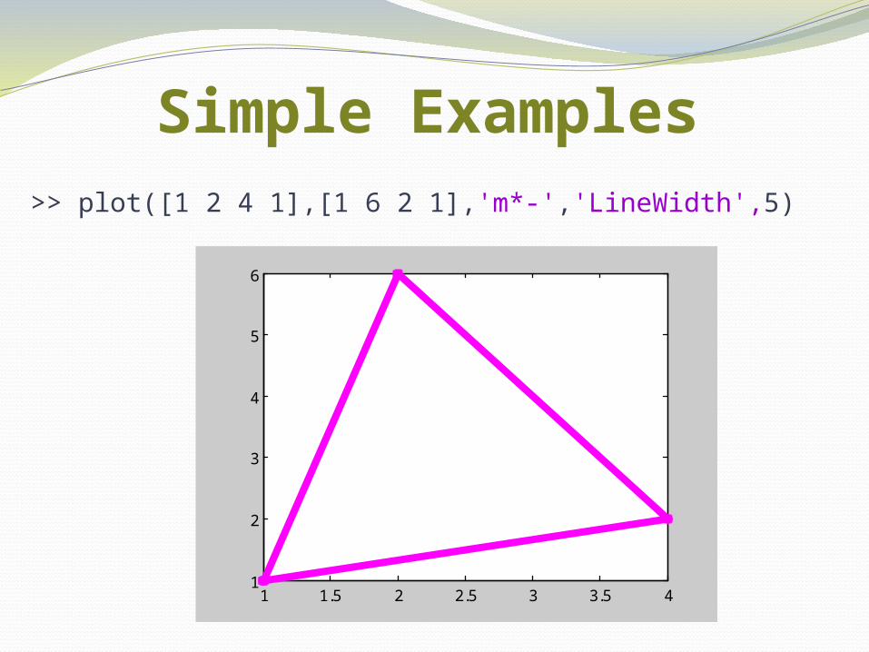
Simple Examples>> plot([1 2 4 1],[1 6 2 1],'m*-','LineWidth',5)

1 1.5 2 2.5 3 3.5 41

2

3

4

5

6

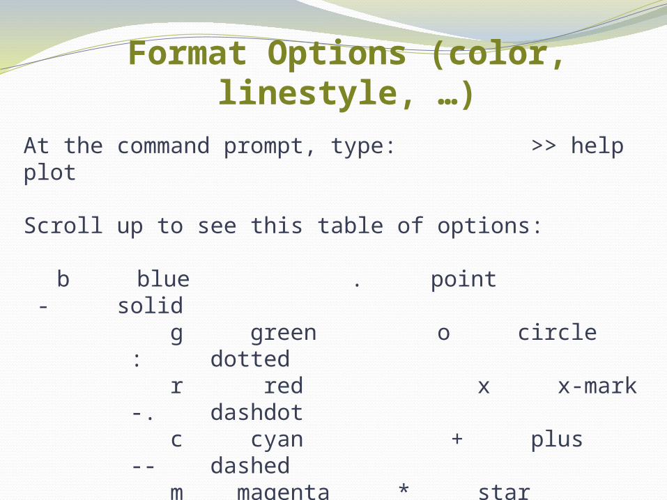
Format Options (color, linestyle, …)At the command prompt, type: >> help plot

Scroll up to see this table of options:

b blue . point - solid g green o circle : dotted r red x x-mark -. dashdot c cyan + plus -- dashed m magenta * star (none) no line y yellow s square k black d diamond w white v triangle (down)

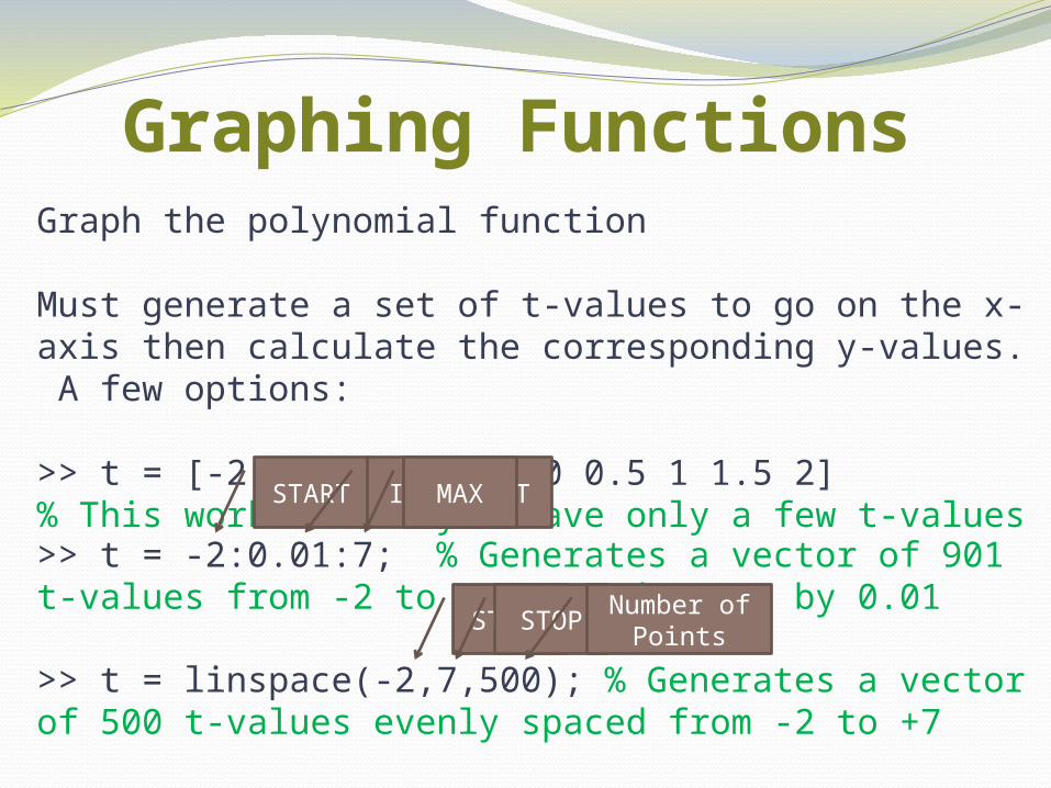
Graphing FunctionsGraph the polynomial function

Must generate a set of t-values to go on the x-axis then calculate the corresponding y-values. A few options:

>> t = [-2 -1.5 -1 -0.5 0 0.5 1 1.5 2] % This works OK if you have only a few t-values

>> t = -2:0.01:7; % Generates a vector of 901 t-values from -2 to +7 spaced apart by 0.01

>> t = linspace(-2,7,500); % Generates a vector of 500 t-values evenly spaced from -2 to +7

START INCREMENTMAX

STARTSTOPNumber of

Points

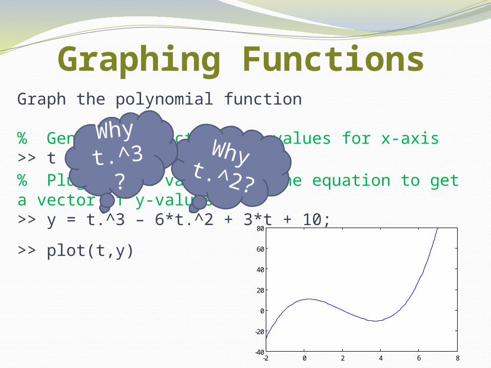
Graphing FunctionsGraph the polynomial function

% Generate a vector of t-values for x-axis>> t = -2:0.01:7;

-2 0 2 4 6 8-40

-20

0

20

40

60

80

% Plug each t value into the equation to get a vector of y-values>> y = t.^3 – 6*t.^2 + 3*t + 10;

>> plot(t,y)

Why t.^2?

Why t.^3?

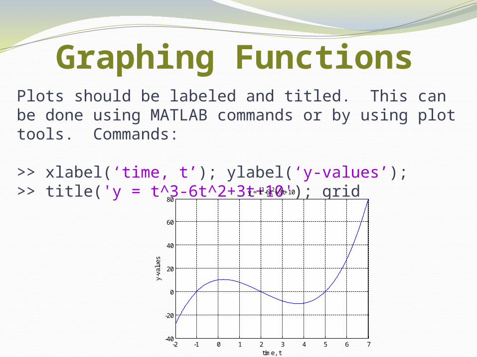
Graphing FunctionsPlots should be labeled and titled. This can be done using MATLAB commands or by using plot tools. Commands:

>> xlabel(‘time, t’); ylabel(‘y-values’);>> title('y = t^3-6t^2+3t+10'); grid

-2 -1 0 1 2 3 4 5 6 7-40

-20

0

20

40

60

80

time, t

y-va

lues

y = t3-6t2+3t+10

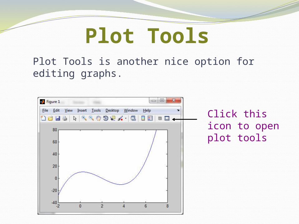
Plot ToolsPlot Tools is another nice option for editing graphs.

Click this icon to open plot tools

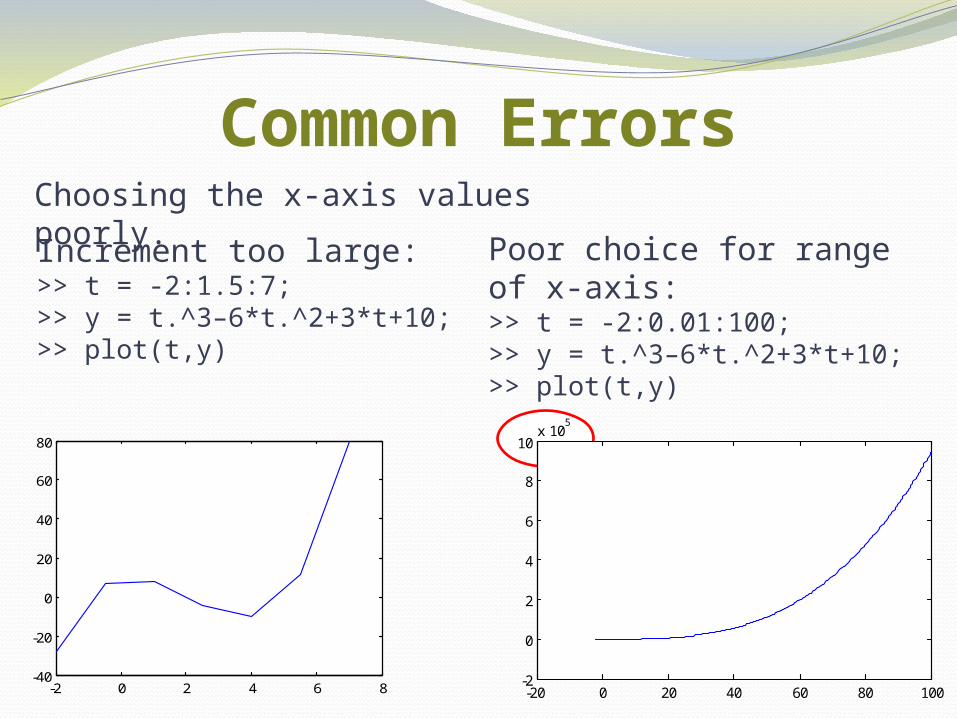
Common Errors

Increment too large:>> t = -2:1.5:7; >> y = t.^3–6*t.^2+3*t+10; >> plot(t,y)

-2 0 2 4 6 8-40

-20

0

20

40

60

80

-20 0 20 40 60 80 100-2

0

2

4

6

8

10x 10

5

Choosing the x-axis values poorly.

Poor choice for range of x-axis:>> t = -2:0.01:100; >> y = t.^3–6*t.^2+3*t+10; >> plot(t,y)

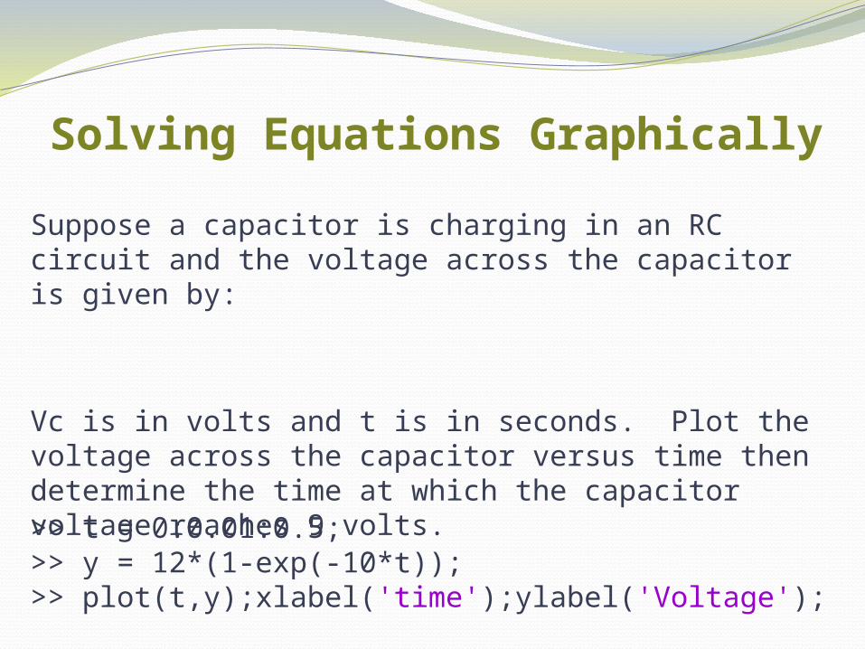
Solving Equations GraphicallySuppose a capacitor is charging in an RC circuit and the voltage across the capacitor is given by:

Vc is in volts and t is in seconds. Plot the voltage across the capacitor versus time then determine the time at which the capacitor voltage reaches 9 volts.

>> t = 0:0.01:0.5; >> y = 12*(1-exp(-10*t));>> plot(t,y);xlabel('time');ylabel('Voltage');

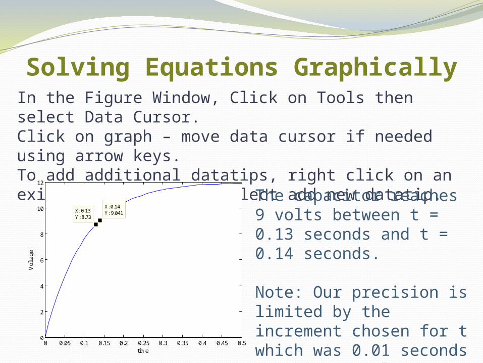
Solving Equations GraphicallyIn the Figure Window, Click on Tools then select Data Cursor.Click on graph – move data cursor if needed using arrow keys.To add additional datatips, right click on an existing datatip and select add new datatip.

0 0.05 0.1 0.15 0.2 0.25 0.3 0.35 0.4 0.45 0.50

2

4

6

8

10

12

X: 0.14Y: 9.041

time

Vol

tage

X: 0.13Y: 8.73

The capacitor reaches 9 volts between t = 0.13 seconds and t = 0.14 seconds.

Note: Our precision is limited by the increment chosen for t which was 0.01 seconds in this example.

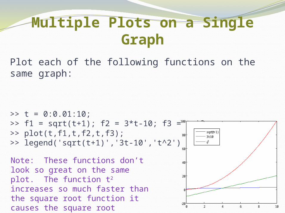
Multiple Plots on a Single GraphPlot each of the following functions on the same graph:

>> t = 0:0.01:10;>> f1 = sqrt(t+1); f2 = 3*t-10; f3 = t.^2;

0 2 4 6 8 10-20

0

20

40

60

80

100

sqrt(t+1)3t-10

t2

Note: These functions don’t look so great on the same plot. The function t2 increases so much faster than the square root function it causes the square root function to look pretty flat.

>> plot(t,f1,t,f2,t,f3);>> legend('sqrt(t+1)','3t-10','t^2')

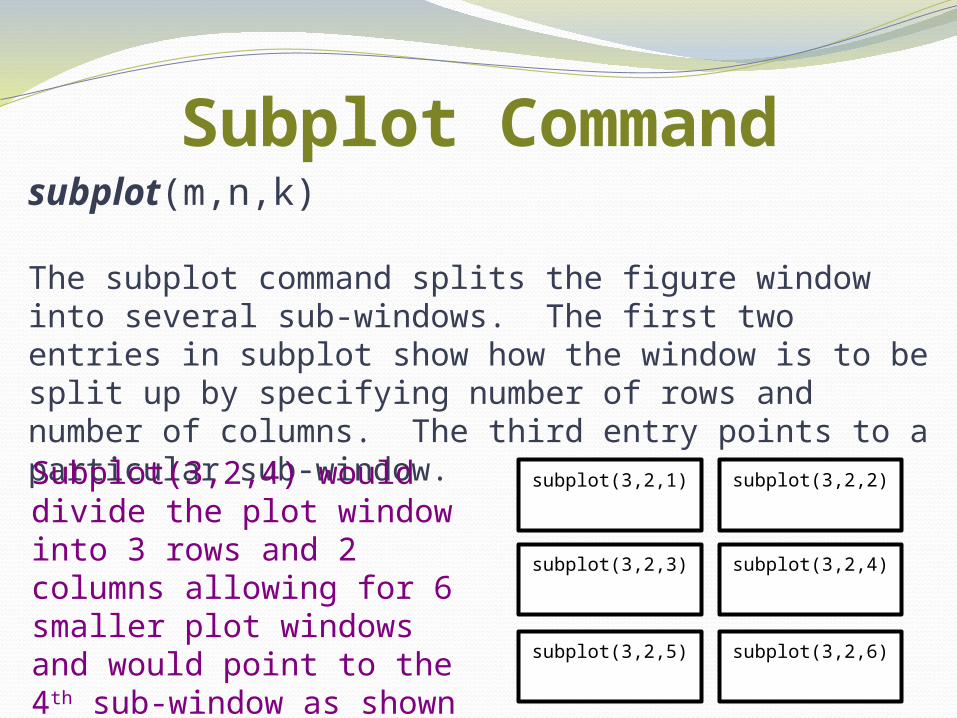
Subplot Commandsubplot(m,n,k)

The subplot command splits the figure window into several sub-windows. The first two entries in subplot show how the window is to be split up by specifying number of rows and number of columns. The third entry points to a particular sub-window.

subplot(3,2,1) subplot(3,2,2)

subplot(3,2,3) subplot(3,2,4)

subplot(3,2,5) subplot(3,2,6)

Subplot(3,2,4) would divide the plot window into 3 rows and 2 columns allowing for 6 smaller plot windows and would point to the 4th sub-window as shown in the diagram.

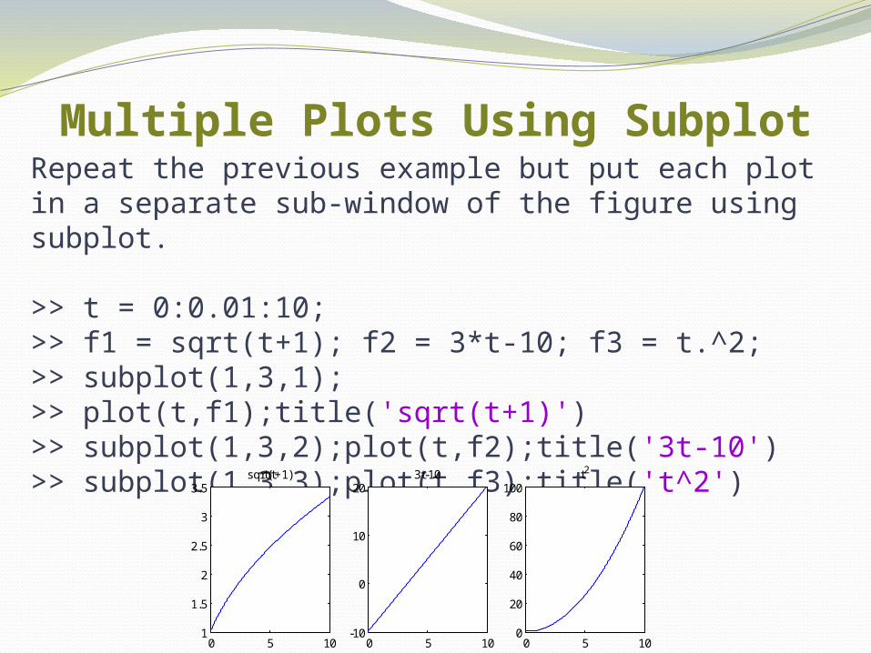
Multiple Plots Using SubplotRepeat the previous example but put each plot in a separate sub-window of the figure using subplot.

>> t = 0:0.01:10;>> f1 = sqrt(t+1); f2 = 3*t-10; f3 = t.^2;>> subplot(1,3,1);>> plot(t,f1);title('sqrt(t+1)')>> subplot(1,3,2);plot(t,f2);title('3t-10')>> subplot(1,3,3);plot(t,f3);title('t^2')

0 5 101

1.5

2

2.5

3

3.5sqrt(t+1)

0 5 10-10

0

10

203t-10

0 5 100

20

40

60

80

100t2

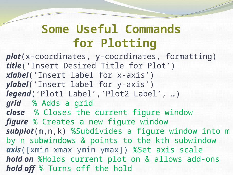
Some Useful Commands for Plotting

plot(x-coordinates, y-coordinates, formatting)title(‘Insert Desired Title for Plot’)xlabel(‘Insert label for x-axis’)ylabel(‘Insert label for y-axis’)legend(‘Plot1 Label’,’Plot2 Label’, …)grid % Adds a gridclose % Closes the current figure windowfigure % Creates a new figure windowsubplot(m,n,k) %Subdivides a figure window into m by n subwindows & points to the kth subwindowaxis([xmin xmax ymin ymax]) %Set axis scale hold on %Holds current plot on & allows add-onshold off % Turns off the hold

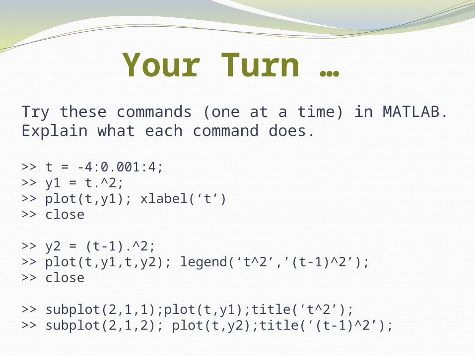
Your Turn …Try these commands (one at a time) in MATLAB. Explain what each command does.

>> t = -4:0.001:4;>> y1 = t.^2;>> plot(t,y1); xlabel(‘t’)>> close

>> y2 = (t-1).^2;>> plot(t,y1,t,y2); legend(‘t^2’,’(t-1)^2’);>> close

>> subplot(2,1,1);plot(t,y1);title(‘t^2’);>> subplot(2,1,2); plot(t,y2);title(‘(t-1)^2’);

Test Your Understanding