Introduction to Harmonic Analysis Basics Course No: E05-009

Credit: 5 PDH

Velimir Lackovic, Char. Eng.

Continuing Education and Development, Inc. 9 Greyridge Farm Court Stony Point, NY 10980 P: (877) 322-5800 F: (877) 322-4774 info@cedengineering.com

Basics of Harmonic Analysis Introduction In this course we will discuss the underlying concepts of harmonic analysis in

relation to industrial and commercial power systems. Also included will be the

reasons we require this analysis, the recognition of problems that may arise in the

process, methods of correcting and preventing these issues, the data required to

perform this analysis, and the benefits of technology in performing a harmonic

analysis study.

The main source of power system harmonics has traditionally been the static power

converter, used as a rectifier in many industrial processes. The static power

converter is now used in a number of different applications. These include adjustable

speed drives, frequency changers for induction heating, switched-mode supplies,

and many more. Increasingly, semiconductor devices are being used as static

switches to adjust the amount of voltage being applied to a load. Some applications

for this include light dimmers, electronic ballasts for discharge lamps, soft starters for

motors, and static var compensators. Any device with a nonlinear voltage current like

an arc furnace or saturable electromagnetic device can also be included.

Nonlinear loads represent a growing portion of the total load of a commercial or

industrial power system. This means harmonic studies are an important part of any

system design and operation. Fortunately, the software available to assist us with

harmonic analysis has grown also.

If we model power system impedances as a function of frequency, we can determine

the effect of harmonic contributions produced by nonlinear loads on voltage and

current in a power system. The majority of harmonic analysis software will offer the

ability to do as follows:

- Calculate harmonic bus voltages and branch current flows produced by

harmonic sources in a network

- See resonances in an existing or planned system

- Calculate the effects of harmonics on voltage or current waveform distortion

or telephone interference through performance indices. This can also aid in

finding capacitors and passive filters to produce optimal system performance.

We will discuss the details of applicable standards and system modelling, particularly

in industrial and commercial systems running at low or medium voltages. The basics

are applicable also to higher voltage systems and other system applications. In this

course, we will not cover active filters as part of a design, but some references will

be made to their use and application.

From the beginning we may say that harmonic filter design is linked closely to power-

factor (PF) requirements in a system, based on utility tariffs. Both must therefore be

considered together. Many studies on PF compensation have previously been made

without considering possible resonances or harmonic absorption by capacitors.

Background By definition, any device or load that doesn’t draw a sinusoidal current when excited

by a sinusoidal voltage of the same frequency is a nonlinear load. Most commonly

these are switching devices like solid-state converters which force conduction of

currents for particular periods. They can also include saturable impedance devices

like transformers with nonlinear voltage vs. impedance characteristics. Nonlinear

loads are also considered sources of harmonic currents, in which harmonic

frequencies are classed as integer multiples of the system frequency. Arc furnaces,

cycloconverters, and other specific nonlinear loads can have non-integer harmonic

frequencies as well as the integer harmonics expected in the system.

Harmonics are a part of every fundamental current cycle. When calculating them,

they are considered part of the steady-state solution. But harmonics can vary from

cycle to cycle, as exceptions will always occur. These are classed as time-varying

harmonics. These are neither dealt with in this chapter, nor are quasisteady-state or

transient solutions (as in magnetization inrush current of a transformer).

In industrial application studies, the nonlinear load or harmonic source is classed as

an ideal current source without a Norton’s impedance (i.e. assume infinite Norton

impedance), providing a constant current, regardless of the system impedance seen

by the source. This is generally a reasonable assumption and tends to yield

acceptable results. A Norton equivalent current source can still be used when a

nonlinear device acts as a voltage source, such as with pulse-width-modulated or

PWM inverters, as most computer software works on the current injection method.

Networks are solved for current and voltage individually at each frequency, as a

system is subjected to current injections at multiple frequencies. Then, the total

voltage or current can be found through a root-mean-square or arithmetic sum via

the principle of superposition.

Different types of nonlinear loads will generate different harmonic frequencies. Most

will produce odd harmonics, with small, even harmonics, but loads like arc furnaces

produce the entire spectrum: odd, even, and non-integer, also known as

interharmonics. In general, the harmonic amplitude will decrease as the harmonic

order or frequency increases.

Depending on harmonic voltage drops in various series elements of the network,

distortion of the voltage waveform is produced due to the effects of harmonic current

propagation through the network (including the power source). Voltage distortion at a

bus depends on the equivalent source impedance – smaller impedance means

better quality voltage. Note that nonlinear loads of harmonic sources are not power

sources, but the cause of active and reactive losses of power in a system.

The Purpose of a Harmonic Study

Nonlinear loads represent a growing propagation in commercial buildings and

industrial plants, in the range of thirty to fifty percent of the total load. This means we

need to examine the effects of harmonics within a system and the impact they have

on a utility and neighbouring loads, to prevent any complaints, equipment damage,

or loss in production.

The list below represents a number of situations in which a harmonic study may be

necessary, including recommendations for mitigation of harmonic effects.

a) IEEE Std. 519-1992 compliance, defining the current distortion limits that

should be met in the utility at the point of common coupling or PCC. As a

basis for the system design, limits of voltage distortion are also defined.

These are intended to provide a good sine wave voltage in the utility, but

users are expected to use them as a basis for the design of a system. If

current distortion limits are met, voltage distortion limits should also be met,

allowing for unusual and exceptional circumstances.

b) Harmonic related problems in the past, including failure of power-factor

compensation capacitors; overheating of transformers, motors, cables, and

other such equipment; and misoperation of protective relays and control

devices.

c) Expansion in which significant nonlinear loads are added, or a significant

capacitance is added to a plant.

d) Designing a new power system or facility in which the power factor

compensation, load-flow, and harmonic analyses need to be studied in one

integrated unit, in order to determine reactive power demands, harmonic

performance limits, and how to meet these requirements. If system problems

appear to be caused by harmonics, it becomes important to determine

resonant frequencies at points which are causing problems. Parallel system

resonance can also occur around the lower harmonic orders (3, 5…) with

banks of power-factor correction capacitors. This can be critical if a harmonic

current injection at that frequency excites the resonance.

Frequently you will find systems where taking harmonic measurements as a tool for

diagnostics rather than performing detailed analysis studies will be a much more

practical task. Measurements can also be used to verify system models before

performing a detailed harmonic analysis study. Arc furnace installations are a

situation in which this is especially desirable. Careful consideration must be given to

procedures and test equipment to make sure harmonic measurements will produce

reliable results. These may produce the cause of a problem, meaning a simpler

study or even the elimination of the need for a study.

Harmonic Sources

Harmonic sources are all considered nonlinear loads, as when a sinusoidal voltage

is applied, they draw non-sinusoidal currents. This may be caused by the inherent

characteristics of the load as in arc furnaces, or due to a switching circuit like a 6-

pulse converter, which forces conduction for particular periods. There may be many

such harmonic sources throughout an industrial or commercial power system.

Harmonic studies require that the performer has knowledge of harmonic currents

produced by the involved nonlinear loads. An analytical engineer has three main

choices.

- Measuring harmonics produced at each source

- Calculating harmonics produced via a mathematic analysis in applicable

situations; e.g. converters or static var compensators

- Using typical values from published data on similar applications

All three of these methods are used in practice and acceptable results are produced

by each.

System configuration and loads are continually changing. This means that the

harmonics also change, and studying all possible conditions would be a difficult task.

Instead, designs are based on the “worst-generated” harmonics, by finding the worst

operating condition available. However, even with this case, harmonic flows through

various parts of a network can be different, depending on tie breakers or

transformers involved. Even with the “worst-generated” case, this means we must

also analyse the “worst operating case(s)”.

When multiple harmonic sources are connected to the same or different buses,

another difficulty arises in the analysis. Phase angles between same order

harmonics are usually unknown. This means that we generally have to turn to

arithmetic addition of harmonic magnitudes, assuming the sources are similar, with

similar operating load points. If sources are different, or operate at different load

points, this approach can produce more conservative filter designs or distortion

calculations. For common industrial applications, determining phase angles of

harmonics and vectorial addition is often not very cost-effective and can be over-

complicated, but this can be resolved by simplifying assumptions through field

measurements or previous experience. When accuracy is more important, such as in

high-voltage DC transmission and other utility applications, more advanced

techniques are employed.

Industrial harmonic studies are usually based on the assumption that a positive

sequence analysis applies, and a system is balanced. This means they are

represented on a single-phase basis. If the system or load is extremely unbalanced,

or a four-wire system exists with single-phase loads, this warrants a three-phase

study. This situation makes it appropriate and preferred to find the harmonics

generated in all three phases. A three phase study, however, may not serve the full

purpose of the study if harmonic generation is assumed to be balanced, while the

system is unbalanced. The cost of one of these studies can be much higher than a

single-phase study, so it should only be used if it is justifiable to produce this

expense for this purpose.

Effects of Harmonics

Harmonic effects are only described here in terms of an analytical study of a

harmonic system. These harmonics influence system losses, operation, and

performance, making them ubiquitous in a power system. If they are not contained

within acceptable limits, harmonics can damage both power and electronic

equipment, resulting in costly system outages.

Harmonic effects are caused by both voltage and current, but the effects of current

are more often seen in a conventional performance. However, degradation of

insulation can be caused by voltage effects, thereby shortening equipment life. The

list below describes some common harmonic effects:

- Losses in equipment, cables, lines, etc.

- Rotating equipment produces pulsating and reduced torque

- Increased stress in equipment insulation causing premature aging

- Rotating and static equipment producing increased audible noise

- Waveform sensitive equipment being misoperated

- Resonances causing significant amplification of voltage and current

- Inductive coupling between power and communication circuits causing

communication interference

Common harmonic studies including harmonic flows and filter design tend not to

involve an in-depth analysis of harmonic effects when the limits of a standard or user

are met, but in some specific cases, a separate study is required for harmonics

penetrating into rotating equipment, affecting communication circuits, or causing

misoperation of relays.

Resonance

Elements of a power system circuit are predominantly inductive. This means the

inclusion of shunt capacitors for power-factor correction or harmonic filtering can

cause inductive and capacitive elements to transfer cyclic energy at the natural

resonance frequency. Inductive and capacitive reactance is equal at this frequency.

When viewed from a bus of interest, commonly the bus where a nonlinear source

injects harmonic currents, the combination of inductive (L) and capacitive (C)

elements can result in either a series resonance (L and C in series) or a parallel

resonance (L and C in parallel). The following sections will show that a series

resonance results in low impedance, while a parallel resonance will result in a high

impedance. The net impedance in either series or parallel is resistive. It is essential

that the driving-point impedance (as seen from the bus of interest) is examined in a

harmonic study, to determine the frequencies of series and parallel resonances, and

their resulting impedances.

PF correction capacitors are commonly used in practical electrical systems to offset

utility-imposed power factor penalties. The combination of capacitors and inductive

elements in the system can result either in series or parallel resonance, or a

combination of both, depending on the system configuration, which can result in an

abnormal situation. Parallel resonance is more common as capacitor banks act in

parallel with inductive system impedance, which can be a problem when the

resonant frequency is close to one of those generated by the harmonic sources.

Series resonance can result in unexpected amounts of harmonic currents flowing

through certain elements. Excessive harmonic current flow can cause inadvertent

relay operation, burned fuses, or overheating of cables.

Parallel resonance may produce excessive harmonic voltage across network

elements. Commonly, this will cause capacitor or insulation failure.

Series Resonance

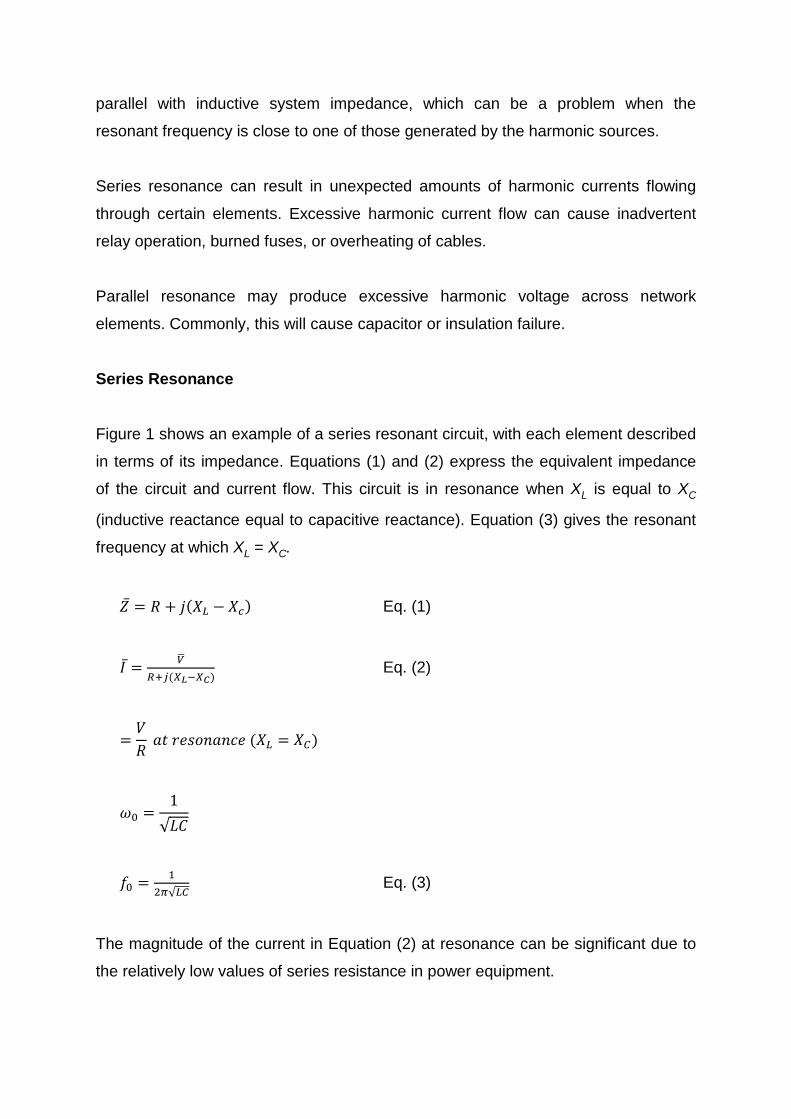
Figure 1 shows an example of a series resonant circuit, with each element described

in terms of its impedance. Equations (1) and (2) express the equivalent impedance

of the circuit and current flow. This circuit is in resonance when XL is equal to XC

(inductive reactance equal to capacitive reactance). Equation (3) gives the resonant

frequency at which XL = XC.

�̅�𝑍 = 𝑅𝑅 + 𝑗𝑗(𝑋𝑋𝐿𝐿 − 𝑋𝑋𝑐𝑐) Eq. (1)

𝐼𝐼 ̅ = 𝑉𝑉�

𝑅𝑅+𝑗𝑗(𝑋𝑋𝐿𝐿−𝑋𝑋𝐶𝐶) Eq. (2)

=𝑉𝑉𝑅𝑅

𝑎𝑎𝑎𝑎 𝑟𝑟𝑟𝑟𝑟𝑟𝑟𝑟𝑟𝑟𝑎𝑎𝑟𝑟𝑟𝑟𝑟𝑟 (𝑋𝑋𝐿𝐿 = 𝑋𝑋𝐶𝐶)

𝜔𝜔0 =1

√𝐿𝐿𝐿𝐿

𝑓𝑓0 = 12𝜋𝜋√𝐿𝐿𝐶𝐶

Eq. (3)

The magnitude of the current in Equation (2) at resonance can be significant due to

the relatively low values of series resistance in power equipment.

R jXL

-jXCV+

-

I

Figure 1. Series resonance circuit example.

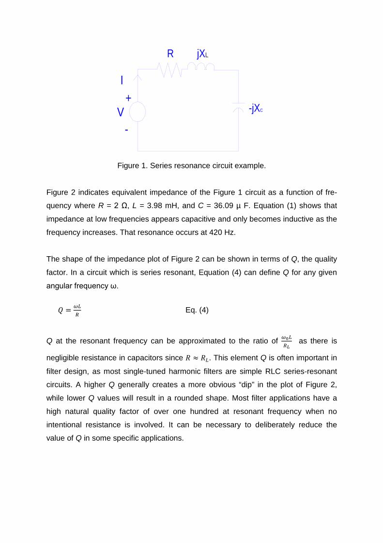
Figure 2 indicates equivalent impedance of the Figure 1 circuit as a function of fre-

quency where R = 2 Ω, L = 3.98 mH, and C = 36.09 µ F. Equation (1) shows that

impedance at low frequencies appears capacitive and only becomes inductive as the

frequency increases. That resonance occurs at 420 Hz.

The shape of the impedance plot of Figure 2 can be shown in terms of Q, the quality

factor. In a circuit which is series resonant, Equation (4) can define Q for any given

angular frequency ω.

𝑄𝑄 = 𝜔𝜔𝐿𝐿

𝑅𝑅 Eq. (4)

Q at the resonant frequency can be approximated to the ratio of 𝜔𝜔0𝐿𝐿𝑅𝑅𝐿𝐿

as there is

negligible resistance in capacitors since 𝑅𝑅 ≈ 𝑅𝑅𝐿𝐿. This element Q is often important in

filter design, as most single-tuned harmonic filters are simple RLC series-resonant

circuits. A higher Q generally creates a more obvious “dip” in the plot of Figure 2,

while lower Q values will result in a rounded shape. Most filter applications have a

high natural quality factor of over one hundred at resonant frequency when no

intentional resistance is involved. It can be necessary to deliberately reduce the

value of Q in some specific applications.

Frequency (Hz)60

Impe

danc

e M

agni

tude

(O

)

0

10

20

30

40

50

60

200 340 480 620 760

70

Figure 2. Impedance magnitude vs. frequency in a series resonant circuit

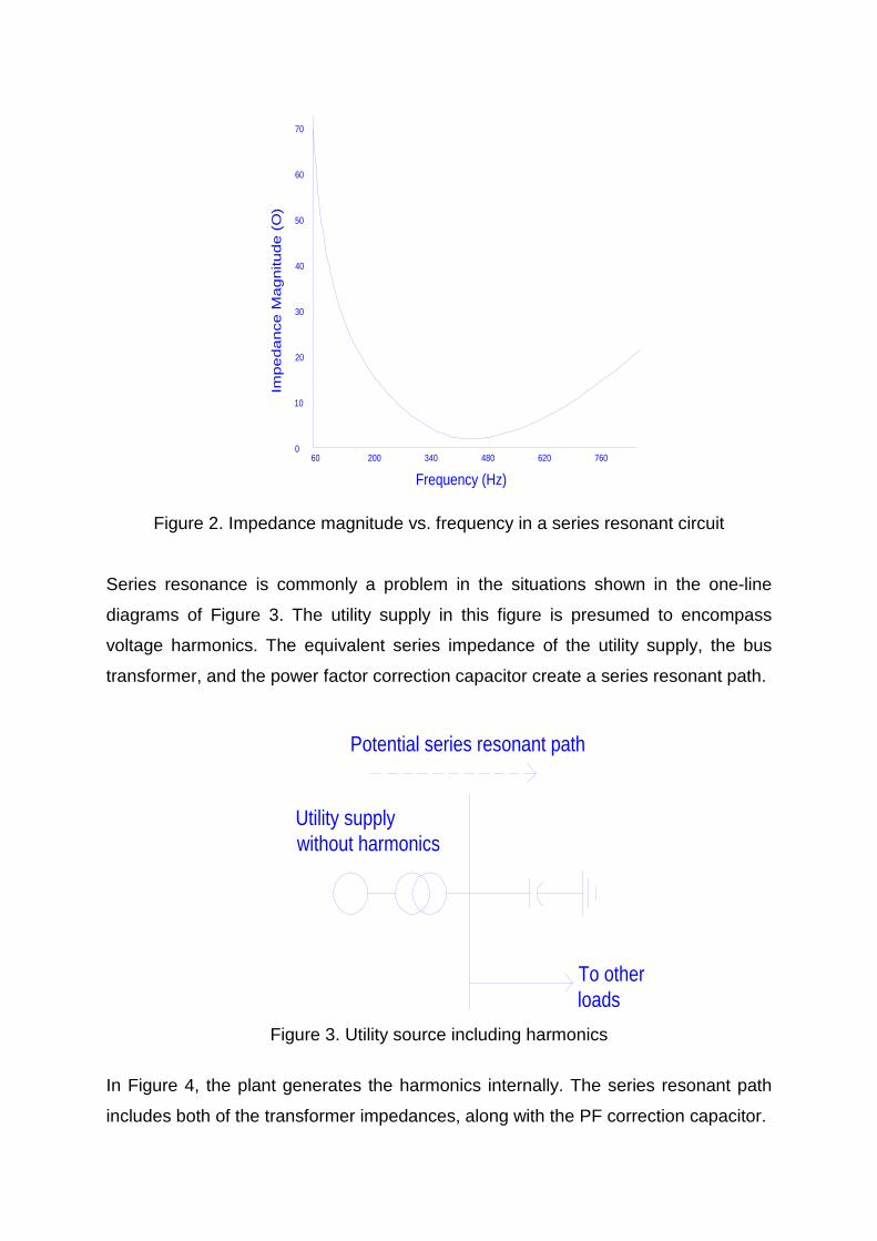
Series resonance is commonly a problem in the situations shown in the one-line

diagrams of Figure 3. The utility supply in this figure is presumed to encompass

voltage harmonics. The equivalent series impedance of the utility supply, the bus

transformer, and the power factor correction capacitor create a series resonant path.

To otherloads

Utility supplywithout harmonics

Potential series resonant path

Figure 3. Utility source including harmonics

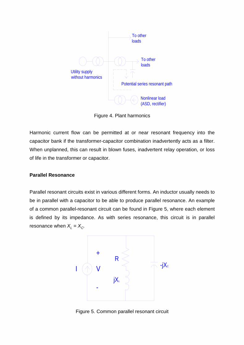
In Figure 4, the plant generates the harmonics internally. The series resonant path

includes both of the transformer impedances, along with the PF correction capacitor.

To otherloads

To otherloads

Nonlinear load(ASD, rectifier)

Utility supplywithout harmonics

Potential series resonant path

Figure 4. Plant harmonics

Harmonic current flow can be permitted at or near resonant frequency into the

capacitor bank if the transformer-capacitor combination inadvertently acts as a filter.

When unplanned, this can result in blown fuses, inadvertent relay operation, or loss

of life in the transformer or capacitor.

Parallel Resonance

Parallel resonant circuits exist in various different forms. An inductor usually needs to

be in parallel with a capacitor to be able to produce parallel resonance. An example

of a common parallel-resonant circuit can be found in Figure 5, where each element

is defined by its impedance. As with series resonance, this circuit is in parallel

resonance when XL = XC.

jXL

R-jXCV

+

-

I

Figure 5. Common parallel resonant circuit

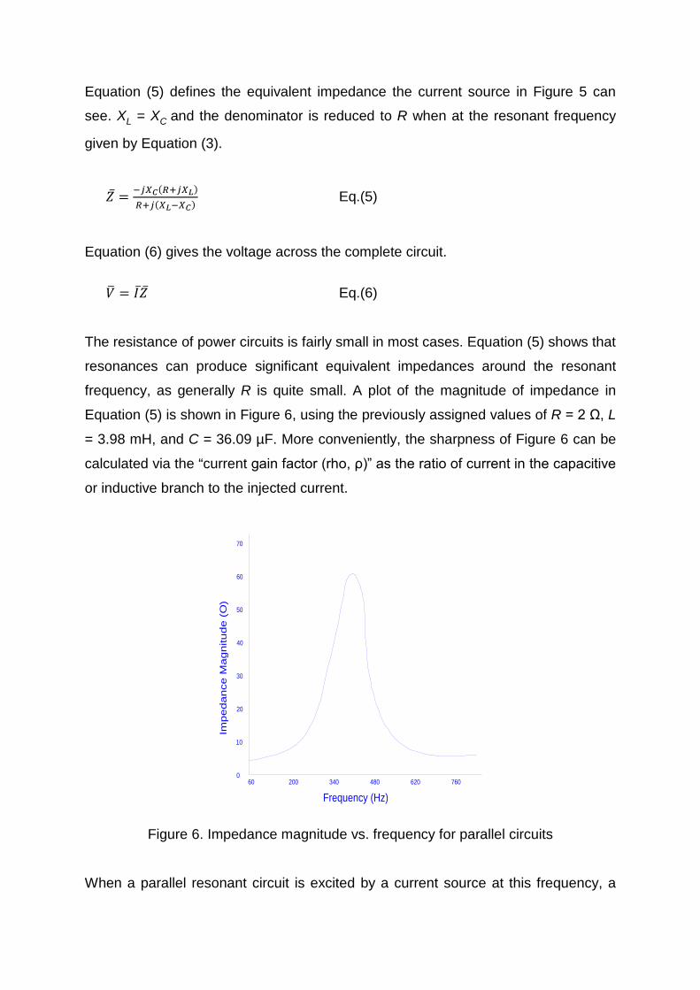
Equation (5) defines the equivalent impedance the current source in Figure 5 can

see. XL = XC and the denominator is reduced to R when at the resonant frequency

given by Equation (3).

�̅�𝑍 = −𝑗𝑗𝑋𝑋𝐶𝐶(𝑅𝑅+𝑗𝑗𝑋𝑋𝐿𝐿)𝑅𝑅+𝑗𝑗(𝑋𝑋𝐿𝐿−𝑋𝑋𝐶𝐶) Eq.(5)

Equation (6) gives the voltage across the complete circuit.

𝑉𝑉� = 𝐼𝐼�̅̅�𝑍 Eq.(6)

The resistance of power circuits is fairly small in most cases. Equation (5) shows that

resonances can produce significant equivalent impedances around the resonant

frequency, as generally R is quite small. A plot of the magnitude of impedance in

Equation (5) is shown in Figure 6, using the previously assigned values of R = 2 Ω, L

= 3.98 mH, and C = 36.09 µF. More conveniently, the sharpness of Figure 6 can be

calculated via the “current gain factor (rho, ρ)” as the ratio of current in the capacitive

or inductive branch to the injected current.

Frequency (Hz)60

Impe

danc

e M

agni

tude

(O

)

0

10

20

30

40

50

60

200 340 480 620 760

70

Figure 6. Impedance magnitude vs. frequency for parallel circuits

When a parallel resonant circuit is excited by a current source at this frequency, a

high circulating current will flow in the capacitance-inductance loop, regardless of the

source current being comparatively small. This is unique to a parallel resonant

circuit. Loop circuit current is amplified dependant purely on the quality factor Q in

the circuit.

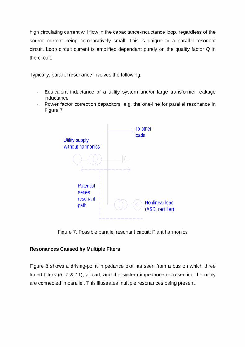
Typically, parallel resonance involves the following:

- Equivalent inductance of a utility system and/or large transformer leakage inductance

- Power factor correction capacitors; e.g. the one-line for parallel resonance in Figure 7

To otherloads

Nonlinear load(ASD, rectifier)

Utility supplywithout harmonics

Potentialseriesresonantpath

Figure 7. Possible parallel resonant circuit: Plant harmonics

Resonances Caused by Multiple Flters

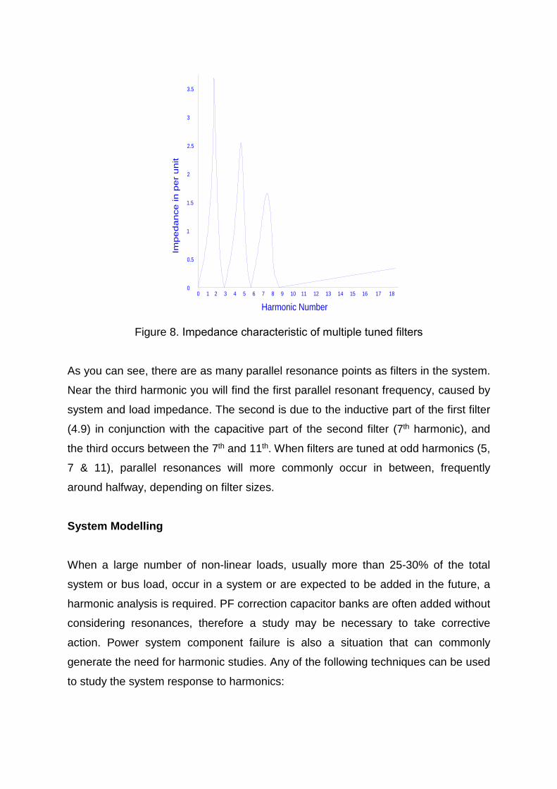
Figure 8 shows a driving-point impedance plot, as seen from a bus on which three

tuned filters (5, 7 & 11), a load, and the system impedance representing the utility

are connected in parallel. This illustrates multiple resonances being present.

Harmonic Number0 1 2 3 4 5 6 7 8 9 10 11 12 13 14 15 16 17 18

Impe

danc

e in

per

uni

t

0

0.5

1

1.5

2

2.5

3

3.5

Figure 8. Impedance characteristic of multiple tuned filters

As you can see, there are as many parallel resonance points as filters in the system.

Near the third harmonic you will find the first parallel resonant frequency, caused by

system and load impedance. The second is due to the inductive part of the first filter

(4.9) in conjunction with the capacitive part of the second filter (7th harmonic), and

the third occurs between the 7th and 11th. When filters are tuned at odd harmonics (5,

7 & 11), parallel resonances will more commonly occur in between, frequently

around halfway, depending on filter sizes.

System Modelling

When a large number of non-linear loads, usually more than 25-30% of the total

system or bus load, occur in a system or are expected to be added in the future, a

harmonic analysis is required. PF correction capacitor banks are often added without

considering resonances, therefore a study may be necessary to take corrective

action. Power system component failure is also a situation that can commonly

generate the need for harmonic studies. Any of the following techniques can be used

to study the system response to harmonics:

- Hand Calculations. Manual calculations can be used, however these are quite

tedious and vulnerable to error, and are therefore restricted to small networks

- Transient Network Analyzer or TNA. These are also kept to smaller networks,

as they are usually time consuming and expensive.

- Field Measurements. Often, harmonic measurements can be used to

establish individual and total harmonic distortions in a system. This can be

done as part of design verification, standard compliance, or field problem

diagnosis. These are effective for validating and refining system modelling in

digital simulations, especially if a parallel resonance is encountered, or non-

characteristic harmonics are present. If using field data for digital simulations

of harmonic current injections, particular attention should be paid if the data

differs significantly from generally acceptable values per unit, or calculated

values. Interharmonic measurements also require special instrumentation and

consideration.

It can be expensive and time-consuming to take harmonic measurements

systematically. They only consider the circumstances in which they were taken,

therefore can’t be guaranteed to reflect the worst possible conditions of a system.

Measurements can also be inaccurate due to measuring errors or flawed use of

instruments.

- Digital Simulation. The most convenient and perhaps economical system

analysis method, as computer technology affords quite advanced programs

with a variety of system component models that can be used in various

different cases. Powerful, elegant numerical calculation techniques work with

the ideas of system impedance and admittance matrices to perform a system-

wide analysis

While they do require additional information for frequency dependence, short-circuit

and load-flow data can be used for harmonic studies. The behaviour of the

equipment involved must be predicted for frequencies above and beyond the current

or usual values. The subclause below provides a summary of system modelling for

harmonic analysis. Assume the models and constants are just examples, as many

others can be substituted.

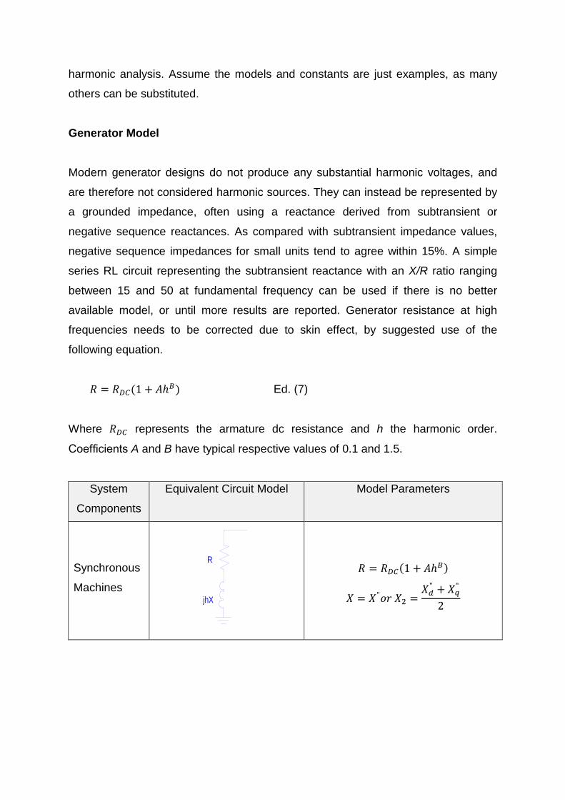
Generator Model

Modern generator designs do not produce any substantial harmonic voltages, and

are therefore not considered harmonic sources. They can instead be represented by

a grounded impedance, often using a reactance derived from subtransient or

negative sequence reactances. As compared with subtransient impedance values,

negative sequence impedances for small units tend to agree within 15%. A simple

series RL circuit representing the subtransient reactance with an X/R ratio ranging

between 15 and 50 at fundamental frequency can be used if there is no better

available model, or until more results are reported. Generator resistance at high

frequencies needs to be corrected due to skin effect, by suggested use of the

following equation.

𝑅𝑅 = 𝑅𝑅𝐷𝐷𝐶𝐶(1 + 𝐴𝐴ℎ𝐵𝐵) Ed. (7)

Where 𝑅𝑅𝐷𝐷𝐶𝐶 represents the armature dc resistance and h the harmonic order.

Coefficients A and B have typical respective values of 0.1 and 1.5.

System

Components

Equivalent Circuit Model Model Parameters

Synchronous

Machines

R

jhX

𝑅𝑅 = 𝑅𝑅𝐷𝐷𝐶𝐶(1 + 𝐴𝐴ℎ𝐵𝐵)

𝑋𝑋 = 𝑋𝑋"𝑟𝑟𝑟𝑟 𝑋𝑋2 =𝑋𝑋𝑑𝑑" + 𝑋𝑋𝑞𝑞"

2

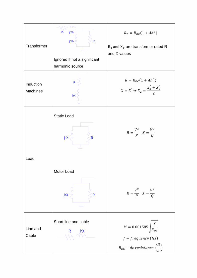
Transformer jhXm Rc

jhXTRT

Ignored if not a significant

harmonic source

𝑅𝑅𝑇𝑇 = 𝑅𝑅𝐷𝐷𝐶𝐶(1 + 𝐴𝐴ℎ𝐵𝐵)

RT and XT are transformer rated R

and X values

Induction

Machines

R

jhX

𝑅𝑅 = 𝑅𝑅𝐷𝐷𝐶𝐶(1 + 𝐴𝐴ℎ𝐵𝐵)

𝑋𝑋 = 𝑋𝑋"𝑟𝑟𝑟𝑟 𝑋𝑋2 =𝑋𝑋𝑑𝑑" + 𝑋𝑋𝑞𝑞"

2

Load

Static Load

jhX R

Motor Load

jhX R

𝑅𝑅 =𝑉𝑉2

𝑃𝑃 𝑋𝑋 =

𝑉𝑉2

𝑄𝑄

𝑅𝑅 =𝑉𝑉2

𝑃𝑃 𝑋𝑋 =

𝑉𝑉2

𝑄𝑄

Line and

Cable

Short line and cable

R jhX

𝑀𝑀 = 0.001585�𝑓𝑓𝑅𝑅𝐷𝐷𝐶𝐶

𝑓𝑓 − 𝑓𝑓𝑟𝑟𝑟𝑟𝑓𝑓𝑓𝑓𝑟𝑟𝑟𝑟𝑟𝑟𝑓𝑓 (𝐻𝐻𝐻𝐻)

𝑅𝑅𝐷𝐷𝐶𝐶 − 𝑑𝑑𝑟𝑟 𝑟𝑟𝑟𝑟𝑟𝑟𝑟𝑟𝑟𝑟𝑎𝑎𝑎𝑎𝑟𝑟𝑟𝑟𝑟𝑟 �𝛺𝛺𝑚𝑚�

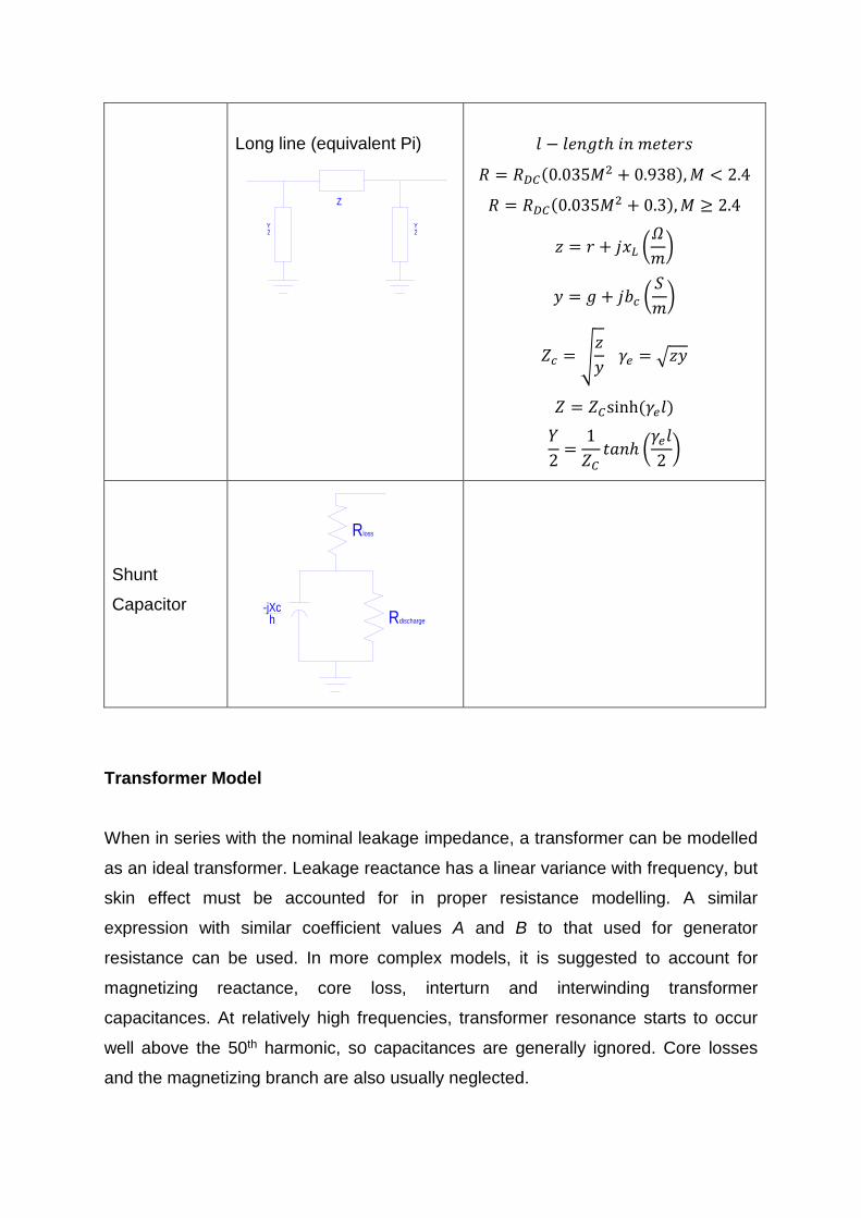
Long line (equivalent Pi)

Z

Y2

Y2

𝑙𝑙 − 𝑙𝑙𝑟𝑟𝑟𝑟𝑙𝑙𝑎𝑎ℎ 𝑟𝑟𝑟𝑟 𝑚𝑚𝑟𝑟𝑎𝑎𝑟𝑟𝑟𝑟𝑟𝑟

𝑅𝑅 = 𝑅𝑅𝐷𝐷𝐶𝐶(0.035𝑀𝑀2 + 0.938),𝑀𝑀 < 2.4

𝑅𝑅 = 𝑅𝑅𝐷𝐷𝐶𝐶(0.035𝑀𝑀2 + 0.3),𝑀𝑀 ≥ 2.4

𝐻𝐻 = 𝑟𝑟 + 𝑗𝑗𝑥𝑥𝐿𝐿 �𝛺𝛺𝑚𝑚�

𝑓𝑓 = 𝑙𝑙 + 𝑗𝑗𝑏𝑏𝑐𝑐 �𝑆𝑆𝑚𝑚�

𝑍𝑍𝑐𝑐 = �𝐻𝐻𝑓𝑓

𝛾𝛾𝑒𝑒 = �𝐻𝐻𝑓𝑓

𝑍𝑍 = 𝑍𝑍𝐶𝐶sinh (𝛾𝛾𝑒𝑒𝑙𝑙) 𝑌𝑌2

=1𝑍𝑍𝐶𝐶𝑎𝑎𝑎𝑎𝑟𝑟ℎ �

𝛾𝛾𝑒𝑒𝑙𝑙2�

Shunt

Capacitor -jXch Rdischarge

Rloss

Transformer Model

When in series with the nominal leakage impedance, a transformer can be modelled

as an ideal transformer. Leakage reactance has a linear variance with frequency, but

skin effect must be accounted for in proper resistance modelling. A similar

expression with similar coefficient values A and B to that used for generator

resistance can be used. In more complex models, it is suggested to account for

magnetizing reactance, core loss, interturn and interwinding transformer

capacitances. At relatively high frequencies, transformer resonance starts to occur

well above the 50th harmonic, so capacitances are generally ignored. Core losses

and the magnetizing branch are also usually neglected.

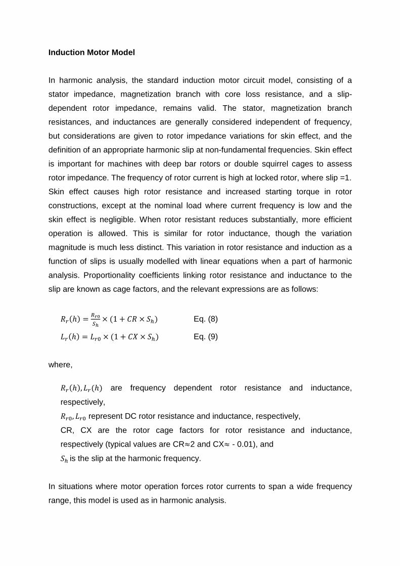
Induction Motor Model

In harmonic analysis, the standard induction motor circuit model, consisting of a

stator impedance, magnetization branch with core loss resistance, and a slip-

dependent rotor impedance, remains valid. The stator, magnetization branch

resistances, and inductances are generally considered independent of frequency,

but considerations are given to rotor impedance variations for skin effect, and the

definition of an appropriate harmonic slip at non-fundamental frequencies. Skin effect

is important for machines with deep bar rotors or double squirrel cages to assess

rotor impedance. The frequency of rotor current is high at locked rotor, where slip =1.

Skin effect causes high rotor resistance and increased starting torque in rotor

constructions, except at the nominal load where current frequency is low and the

skin effect is negligible. When rotor resistant reduces substantially, more efficient

operation is allowed. This is similar for rotor inductance, though the variation

magnitude is much less distinct. This variation in rotor resistance and induction as a

function of slips is usually modelled with linear equations when a part of harmonic

analysis. Proportionality coefficients linking rotor resistance and inductance to the

slip are known as cage factors, and the relevant expressions are as follows:

𝑅𝑅𝑟𝑟(ℎ) = 𝑅𝑅𝑟𝑟0𝑆𝑆ℎ

× (1 + 𝐿𝐿𝑅𝑅 × 𝑆𝑆ℎ) Eq. (8)

𝐿𝐿𝑟𝑟(ℎ) = 𝐿𝐿𝑟𝑟0 × (1 + 𝐿𝐿𝑋𝑋 × 𝑆𝑆ℎ) Eq. (9)

where,

𝑅𝑅𝑟𝑟(ℎ),𝐿𝐿𝑟𝑟(ℎ) are frequency dependent rotor resistance and inductance,

respectively,

𝑅𝑅𝑟𝑟0, 𝐿𝐿𝑟𝑟0 represent DC rotor resistance and inductance, respectively,

CR, CX are the rotor cage factors for rotor resistance and inductance,

respectively (typical values are CR≈2 and CX≈ - 0.01), and

𝑆𝑆ℎ is the slip at the harmonic frequency.

In situations where motor operation forces rotor currents to span a wide frequency

range, this model is used as in harmonic analysis.

Each element of the harmonic current (1h) flowing into a motor will see any

impedance whose value is defined as per the equations above, at the appropriate

slip. For that slip value (𝑆𝑆ℎ) the first expression of the value is obtained from the

basic slip definition, where the slip is the difference between the stator or harmonic

frequency and the rotor electrical frequency, divided by the stator frequency.

𝑆𝑆ℎ = 𝜔𝜔ℎ−𝜔𝜔𝑟𝑟𝜔𝜔ℎ

= ℎ×𝜔𝜔0−(1−𝑠𝑠)×𝜔𝜔0ℎ×𝜔𝜔0

= ℎ+𝑠𝑠−1ℎ

≅ ℎ−1ℎ

Eg. (10)

where,

h is the harmonic order,

𝜔𝜔ℎ,𝜔𝜔𝑟𝑟 ,𝜔𝜔0 are the harmonic angular frequency, rotor angular frequency, and syn-

chronous frequency, respectively, and

𝑆𝑆 is the conventional slip at fundamental frequency.

At higher harmonic orders, we notice that harmonic slip approaches 1, while

resistance and inductance become constants. The harmonic slip can be considered

1 for any harmonic order greater than 9 when used in practice.

Balanced harmonic currents of order Nk + 1, Nk + 2, and Nk + 3 (k = 0, 1, 2 for N =

1, 2, 3…) have been associated with the positive, negative, and zero sequences,

respectively. A negative sequence flux will rotate opposite to the rotor direction, and

the rotor flux frequency can be defined as the sum of the rotor and stator

frequencies. By replacing the minus sign in the harmonic slip expression, we can

take this into account, as shown below.

𝑆𝑆ℎ ≅ℎ±1ℎ

Eq. (11)

where,

“–” is applied to positive sequence harmonics,

“+” is applied to negative sequence harmonics, and

𝑆𝑆ℎ = 1 for zero sequence harmonics.

At higher frequencies, the magnitude of the harmonic slip approaches unity, and we

can approximate the motor inductance using its locked rotor or subtransient value.

Load Model

There have been various models proposed to denote individual and aggregate loads

in harmonic study. There are specific models available for any individual load,

regardless of whether they are passive, rotating, solid-state, or otherwise. Aggregate

loads are usually represented as a parallel or series combination of inductances and

resistances. These are produced as estimated values based on the load power at

fundamental frequency. Using this model we can show aggregates of passive or

motor loads. Resistance and inductances are considered constant over the range of

involved frequencies in this model.

Transmission Line and Cable Models

A series RL circuit denoting the line series resistance and reactance can be used to

represent a short line or cable, but the resistance needs to be corrected for skin

effect at higher frequencies. Modelling the line shunt capacitance becomes

necessary with longer lines. Lumped parameter models like the equivalent pi model,

or distributed parameter models can both be used for this task. The latter is generally

more representative of the line response when used over a wide range of

frequencies. Cascading several lumped parameter models will approximate the

distributed line model. In either model, it is worthwhile to cascade sections to

represent a long line, as this produces a better profile of harmonic voltage along the

line.

The following expression can be used to evaluate the variation in line resistance

caused by skin effect:

𝑅𝑅 = 𝑅𝑅𝑑𝑑𝑐𝑐(0.35𝑋𝑋2 + 0.938),𝑋𝑋 < 2.4 Eq. (12)

𝑅𝑅 = 𝑅𝑅𝑑𝑑𝑐𝑐(0.35𝑋𝑋 + 0.3),𝑋𝑋 ≥ 2.4 Eq. (13)

where,

𝑋𝑋 = 0.001585 � 𝑓𝑓𝑅𝑅𝑑𝑑𝑑𝑑�0.5

,

f is frequency in Hz, and 𝑅𝑅𝑑𝑑𝑐𝑐 is in Ω/mi.

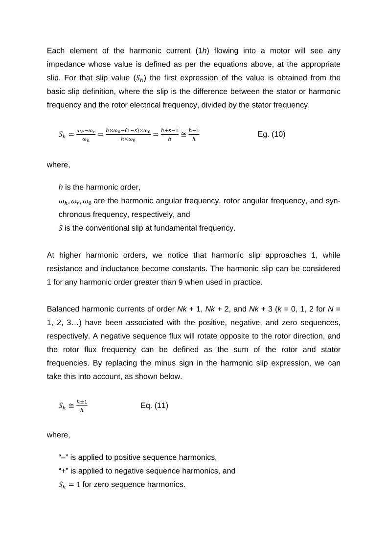
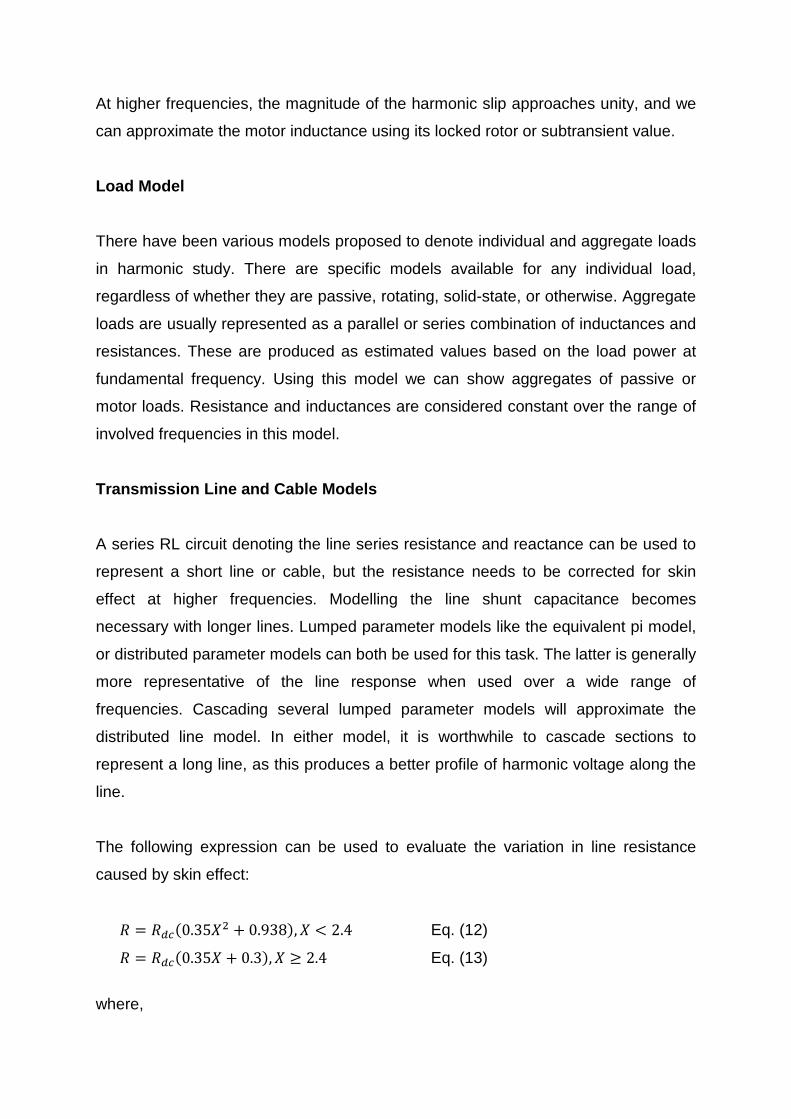
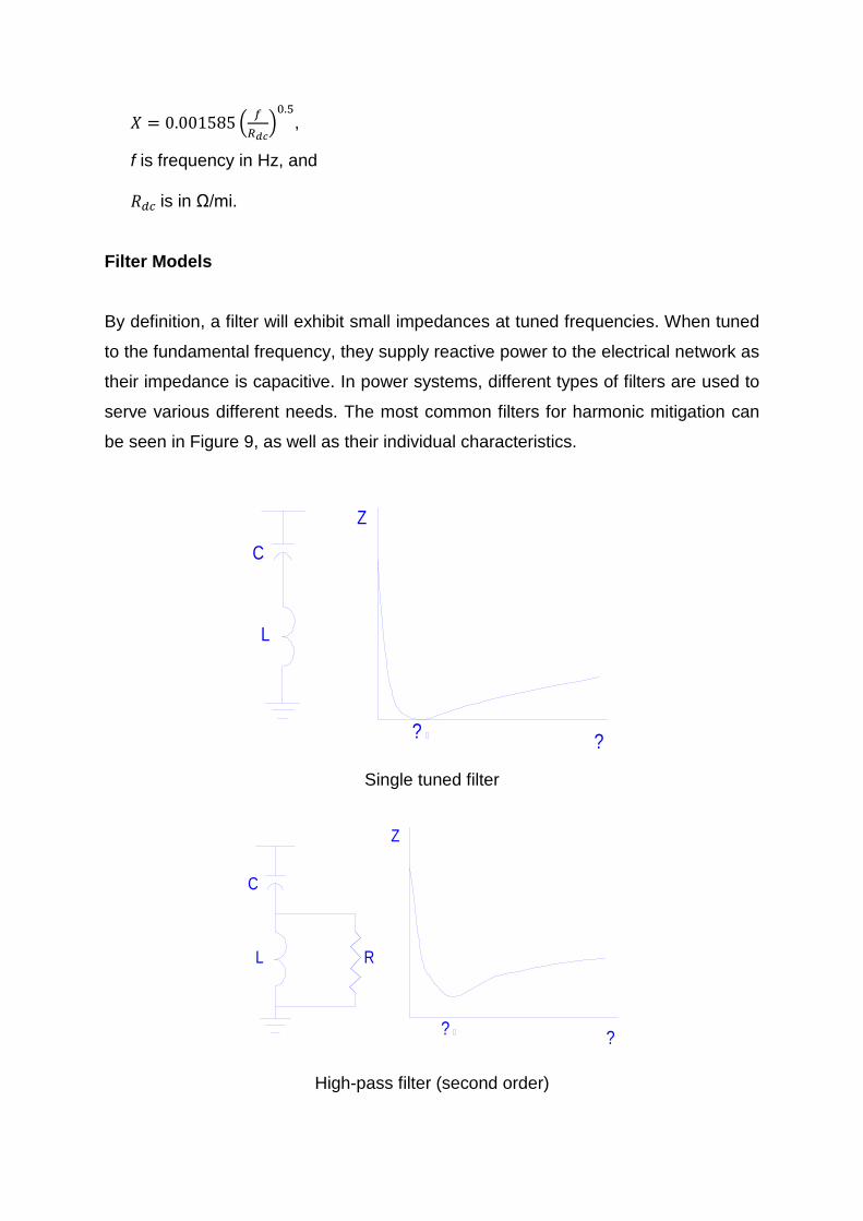
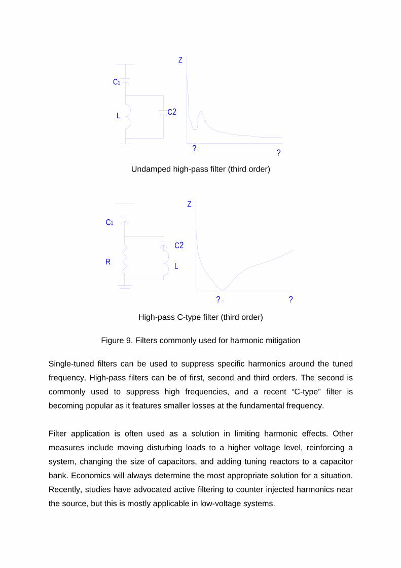
Filter Models

By definition, a filter will exhibit small impedances at tuned frequencies. When tuned

to the fundamental frequency, they supply reactive power to the electrical network as

their impedance is capacitive. In power systems, different types of filters are used to

serve various different needs. The most common filters for harmonic mitigation can

be seen in Figure 9, as well as their individual characteristics.

Z

? ?

C

L

Single tuned filter

Z

? ?

C

L R

High-pass filter (second order)

Z

? ?

C1

L C2

Undamped high-pass filter (third order)

C1

R

C2

L

Z

? ? High-pass C-type filter (third order)

Figure 9. Filters commonly used for harmonic mitigation

Single-tuned filters can be used to suppress specific harmonics around the tuned

frequency. High-pass filters can be of first, second and third orders. The second is

commonly used to suppress high frequencies, and a recent “C-type” filter is

becoming popular as it features smaller losses at the fundamental frequency.

Filter application is often used as a solution in limiting harmonic effects. Other

measures include moving disturbing loads to a higher voltage level, reinforcing a

system, changing the size of capacitors, and adding tuning reactors to a capacitor

bank. Economics will always determine the most appropriate solution for a situation.

Recently, studies have advocated active filtering to counter injected harmonics near

the source, but this is mostly applicable in low-voltage systems.

Network Modelling and Computer-Based Solution Techniques

The most common methodology of harmonic analysis, although several others have

also been used successfully, is the current injection method. This models nonlinear

loads as ideal harmonic sources, and represents each network element with a set of

linear equations corresponding to its previously described circuit. Ohm’s law and

Kirchoff’s laws connect all network elements and loads according to the network

topology. Mathematically, this means each bus of the network holds an equation. So

at bus i, connected to a set of buses j, we have the following:

�∑ 𝑌𝑌𝑖𝑖𝑗𝑗𝑗𝑗 � × 𝑉𝑉𝑖𝑖 = 𝐼𝐼𝑖𝑖 + ∑ �𝑌𝑌𝑖𝑖𝑗𝑗 × 𝑉𝑉𝑗𝑗�𝑗𝑗 Eq. (14)

By solving this system of equations, we obtain the nodal voltages. This computation

is performed for each harmonic frequency of interest. From the harmonic voltages

we can compute the harmonic currents in each branch:

𝐼𝐼𝑖𝑖𝑗𝑗 = �𝑉𝑉𝑖𝑖 − 𝑉𝑉𝑗𝑗� × 𝑌𝑌𝑖𝑖𝑗𝑗 Eq. (15)

Most of the work involved comes from forming the network equations. There are

excellent linear equation solvers available.

The inverse of the nodal admittance matrix is known as the nodal impedance matrix,

and is full of quantitative information. The diagonal entry on the Ith row is known as

the Thevenin impedance of the network, as seen by bus i. We can obtain the

frequency response of a network from each bus by computing these matrix values

over a range of frequencies. This computation can be used to obtain exact resonant

frequencies. In this matrix, off-diagonal values show the effect on bus voltages of a

harmonic current injection.

The total harmonic distortion, rms value, telephone interference factor, and related

factors 𝑉𝑉𝑉𝑉 and 𝐼𝐼𝑉𝑉 are computed from the harmonic voltage or current (𝑈𝑈𝑛𝑛) and the

fundamental frequency (𝑈𝑈1) quantities as below.

Total harmonic distortion (THD) = 100 �∑ 𝑉𝑉𝑛𝑛2∞

𝑛𝑛=2

𝑉𝑉1 Eq. (16)

where n is the harmonic order and usually the summation is made up to the 25th or

50th harmonic order.

rms value: 𝑈𝑈𝑟𝑟𝑟𝑟𝑠𝑠 = �∑ 𝑉𝑉𝑛𝑛2∞𝑛𝑛=1 Eq. (17)

VT or IT: 𝑈𝑈𝑉𝑉 = �∑ �𝐾𝐾𝑓𝑓 × 𝑃𝑃𝑓𝑓 × 𝑉𝑉𝑓𝑓�2∞

𝑓𝑓=0 Eq. (18)

where U designates either voltage or current.

Telephone interference factor: 𝑉𝑉𝐼𝐼𝑇𝑇 =�∑ �𝐾𝐾𝑓𝑓×𝑃𝑃𝑓𝑓×𝑉𝑉𝑓𝑓�

2∞𝑓𝑓=0

𝑉𝑉 Eq. (19)

where V is the voltage and 𝐾𝐾𝑓𝑓 and 𝑃𝑃𝑓𝑓 are the weighting factors related to hearing

sensitivity. These quantities are useful in summarizing a harmonic analysis into

quality-related factors.

Two impedance calculations are made in a harmonic analysis to study system

characteristics in both series and parallel resonances. These are the driving point

and transfer impedances. Driving point impedance is defined by voltage at a node i

due to current injected at the same node, otherwise use:

𝑍𝑍𝑖𝑖𝑖𝑖 = 𝑉𝑉𝑖𝑖𝐼𝐼𝑖𝑖

Eq. (20)

As this is the net impedance of circuits from that bus, useful information on

resonances can be acquired. Changing the locations of capacitors, cables etc. in a

circuit, or the design of planned filters, can change the driving point impedance and

therefore the resonance etc. Transfer impedance is similar to driving point

impedance in the sense that it is the voltage measured at a bus due to injected

current at another bus; in other words:

𝑍𝑍𝑖𝑖𝑗𝑗 = 𝑉𝑉𝑖𝑖𝐼𝐼𝑗𝑗

Eq. (21)

where,

𝑍𝑍𝑖𝑖𝑗𝑗 is the transfer impedance to bus i,

𝑉𝑉𝑖𝑖 is the voltage measured at bus i,

𝐼𝐼𝑗𝑗 is the current injected at bus j.

This is useful when evaluating harmonic voltages at any bus other than the one

where the current is injected.

Harmonic Analysis for Industrial and Commercial Systems

The following list summarizes the steps a harmonic study consists of in the industrial

environment:

- Prepare a system one-line diagram. Be sure to include capacitor banks, long

lines and cables within the industrial or utility system near the point of

common coupling (PCC).

- Collect data and ratings for equipment.

- Obtain nonlinear load locations and generated harmonic currents.

- From the utility company, collect the necessary data and harmonic

requirements at the PCC. These should include the following:

o System impedances, or minimum and maximum fault levels, as a function

of frequency for various system conditions.

o Acceptable harmonic limits, including distortion factors and IT factor.

Criteria and limits vary considerably around the world.

- Carry out harmonic analysis for the base system configuration, through

calculation of the driving point impedance loci at harmonic source buses, and

all shunt capacitor locations.

- Compute individual and total harmonic voltage, current distortion factors, and

IT values if applicable, at the point of common coupling.

- Examine the results, and return to the first or third step, depending whether

the network data or parameters of the analysis need to be changed.

- Compare the composite (fundamental plus harmonic) shunt capacitor bank

loading requirements with the maximum rating permitted by the applicable

standards.

- Relocate the capacitors or change the bank ratings if they exceed the

necessary ratings. If a resonance condition is found, apply a detuning reactor.

(Note that adding a tuning reactor will increase the fundamental voltage on

the capacitor and may also increase harmonic voltage.)

- If the harmonic distortion factors and IT values at the PCC exceed the limit

imposed by the utility, add more filters.

These steps should be followed both for the base system configuration and any

system topologies resulting from likely contingencies. System expansions and short-

circuit level changes in the future should also be taken into consideration in the

process.

Data for Analysis

For a typical study, the following data is required:

- A single-line diagram of the power system in question.

- The short-circuit capacity and X/R ratio of the utility power supply system, and

the existing harmonic voltage spectrum at the PCC (external to the system

being modeled).

- Subtransient reactance and kVA of any rotating machines. If limitations exist,

one composite equivalent machine can be formed from all the machines on a

given bus.

- Reactance and resistance of cables, lines, bus work, current limiting reactors,

and the rated voltage of the circuit the element belongs to. These units can be

presented in per-unit or percent values, or ohmic values, depending on

preference or software usage.

- The three-phase connections, percent impedance, and kVA of all power

transformers.

- The three-phase connections, kvar, and unit kV ratings of all shunt and

reactors.

- Nameplate ratings, number of phases, pulses, and converter connections,

whether they are diodes or thyristors, and, if thyristors, the maximum phase

delay angle per unit loading, and loading cycle of each converter unit involved

in the system. Manufacturer’s test sheets for each converter transformer are

helpful but not mandatory. If this information is not readily available, the kVA

rating of the converter transformer can be used to establish the harmonic

current spectrum being injected into the system.

- Specific system configurations.

- Maximum expected voltage for the nonlinear load system.

- In the case of arc furnace installations, secondary lead impedance from the

transformer to the electrodes, plus a loading cycle to include arc megawatts,

secondary voltages, secondary current furnace transformer taps, and

transformer connections.

- Utility-imposed harmonic limits at the PCC, otherwise limits specified in

applicable standards may be used.

Example Solutions

In this section, several applications of harmonic studies will be discussed. Frequency

scans, capacitor effects, and filter design will be established.

Test System Single-Line Diagram and Data

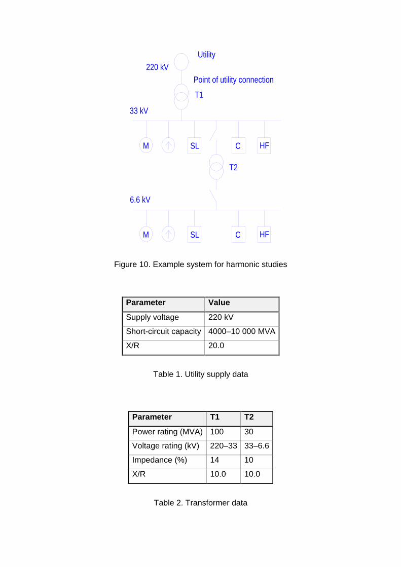
Figure 10 will be used for all examples, as the system in this diagram is

representative of a common industrial power system, including power factor

correction capacitors and voltage levels. Tables 1, 2 and 3 include the necessary

data for a basic harmonic study.

M

33 kV

T1

220 kVUtility

Point of utility connection

6.6 kV

M

SL

T2

C HF

SL C HF

Figure 10. Example system for harmonic studies

Parameter Value

Supply voltage 220 kV

Short-circuit capacity 4000–10 000 MVA

X/R 20.0

Table 1. Utility supply data

Parameter T1 T2

Power rating (MVA) 100 30

Voltage rating (kV) 220–33 33–6.6

Impedance (%) 14 10

X/R 10.0 10.0

Table 2. Transformer data

Load Type Value

33 kV bus

Linear load 25 MVA @ 0.8 lag

Converter 25 MW

Capacitor 8.4 Mvar

6.6 kV bus

Linear load 15 MVA @ 0.8 lag

Converter 15 MW

Capacitor 5 Mvar

Table 3. Load and capacitor data

These capacitor banks have been designed to output a power factor of 0.95, lagging

at the low-voltage side of each transformer. They may consist of both series and

parallel units. The modelling of harmonic studies is, in most cases, not entirely

different from static load. Table 3 therefore includes both types for each bus.

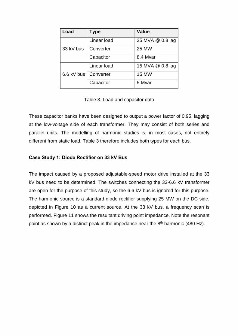
Case Study 1: Diode Rectifier on 33 kV Bus

The impact caused by a proposed adjustable-speed motor drive installed at the 33

kV bus need to be determined. The switches connecting the 33-6.6 kV transformer

are open for the purpose of this study, so the 6.6 kV bus is ignored for this purpose.

The harmonic source is a standard diode rectifier supplying 25 MW on the DC side,

depicted in Figure 10 as a current source. At the 33 kV bus, a frequency scan is

performed. Figure 11 shows the resultant driving point impedance. Note the resonant

point as shown by a distinct peak in the impedance near the 8th harmonic (480 Hz).

Harmonic Number0 1 2 3 4 5 6 7 8 9 10 11 12 13 14 15 16 17 18

Driv

ing

Poi

nt Im

peda

nce

(O)

0

5

10

15

20

25

30

Figure 11. Driving point impedance at 33 kV bus

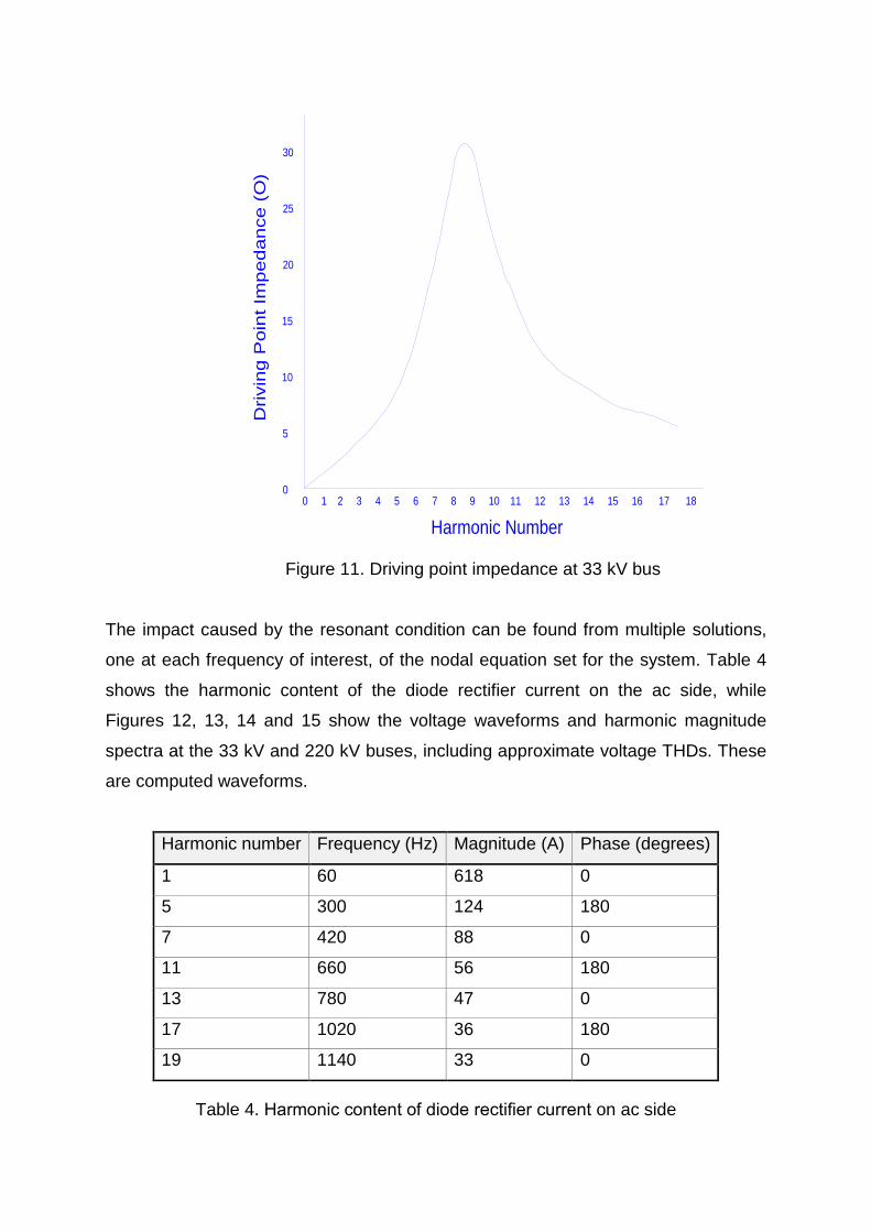
The impact caused by the resonant condition can be found from multiple solutions,

one at each frequency of interest, of the nodal equation set for the system. Table 4

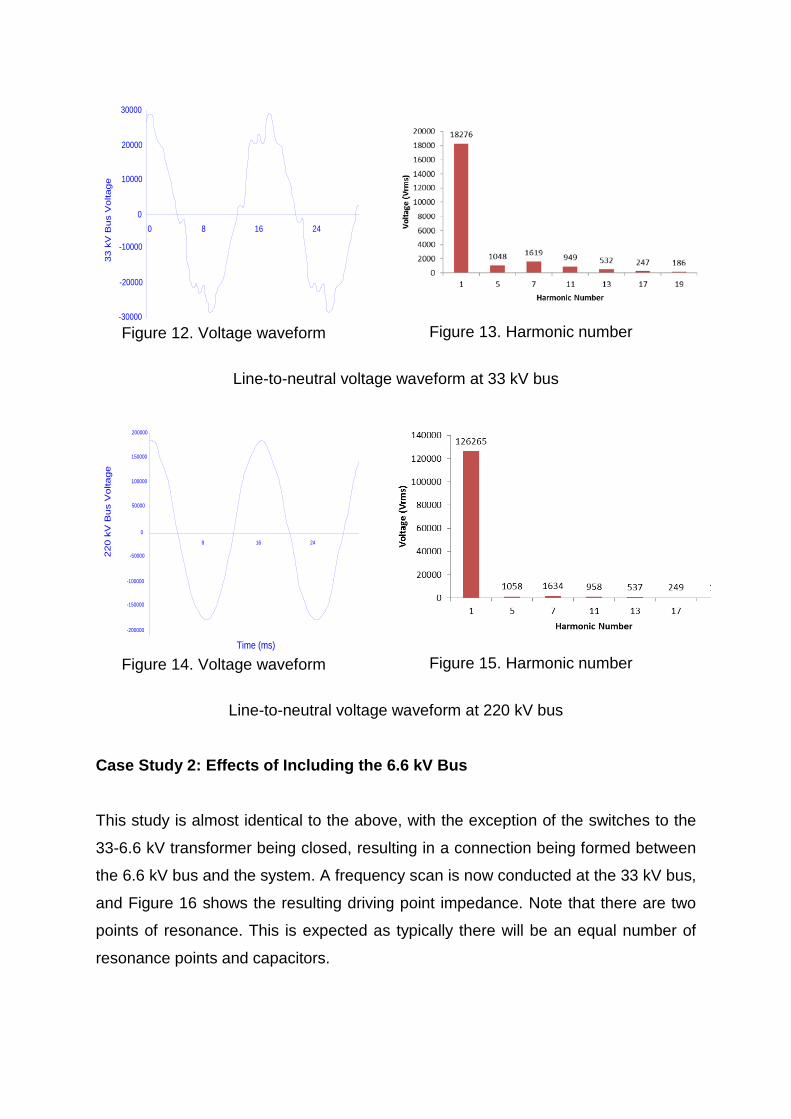
shows the harmonic content of the diode rectifier current on the ac side, while

Figures 12, 13, 14 and 15 show the voltage waveforms and harmonic magnitude

spectra at the 33 kV and 220 kV buses, including approximate voltage THDs. These

are computed waveforms.

Harmonic number Frequency (Hz) Magnitude (A) Phase (degrees)

1 60 618 0

5 300 124 180

7 420 88 0

11 660 56 180

13 780 47 0

17 1020 36 180

19 1140 33 0

Table 4. Harmonic content of diode rectifier current on ac side

0

10000

20000

30000

-10000

-20000

-30000

0 8 16 24

33 k

V B

us V

olta

ge

Figure 12. Voltage waveform

Figure 13. Harmonic number

Line-to-neutral voltage waveform at 33 kV bus

8 16 24

Time (ms)

0

220

kV B

us V

olta

ge

50000

100000

150000

200000

-50000

-100000

-150000

-200000

Figure 14. Voltage waveform

Figure 15. Harmonic number

Line-to-neutral voltage waveform at 220 kV bus

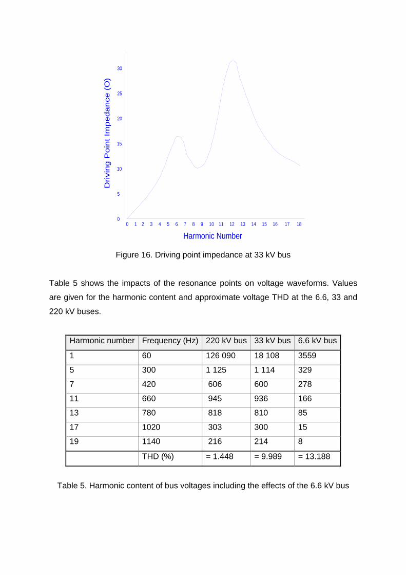
Case Study 2: Effects of Including the 6.6 kV Bus

This study is almost identical to the above, with the exception of the switches to the

33-6.6 kV transformer being closed, resulting in a connection being formed between

the 6.6 kV bus and the system. A frequency scan is now conducted at the 33 kV bus,

and Figure 16 shows the resulting driving point impedance. Note that there are two

points of resonance. This is expected as typically there will be an equal number of

resonance points and capacitors.

Harmonic Number0 1 2 3 4 5 6 7 8 9 10 11 12 13 14 15 16 17 18

Driv

ing

Poi

nt Im

peda

nce

(O)

0

5

10

15

20

25

30

Figure 16. Driving point impedance at 33 kV bus

Table 5 shows the impacts of the resonance points on voltage waveforms. Values

are given for the harmonic content and approximate voltage THD at the 6.6, 33 and

220 kV buses.

Harmonic number Frequency (Hz) 220 kV bus 33 kV bus 6.6 kV bus

1 60 126 090 18 108 3559

5 300 1 125 1 114 329

7 420 606 600 278

11 660 945 936 166

13 780 818 810 85

17 1020 303 300 15

19 1140 216 214 8

THD (%) = 1.448 = 9.989 = 13.188

Table 5. Harmonic content of bus voltages including the effects of the 6.6 kV bus

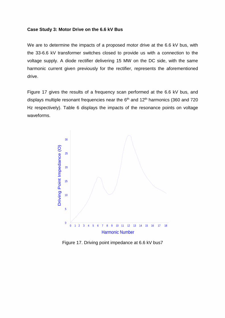
Case Study 3: Motor Drive on the 6.6 kV Bus

We are to determine the impacts of a proposed motor drive at the 6.6 kV bus, with

the 33-6.6 kV transformer switches closed to provide us with a connection to the

voltage supply. A diode rectifier delivering 15 MW on the DC side, with the same

harmonic current given previously for the rectifier, represents the aforementioned

drive.

Figure 17 gives the results of a frequency scan performed at the 6.6 kV bus, and

displays multiple resonant frequencies near the 6th and 12th harmonics (360 and 720

Hz respectively). Table 6 displays the impacts of the resonance points on voltage

waveforms.

Harmonic Number0 1 2 3 4 5 6 7 8 9 10 11 12 13 14 15 16 17 18

Driv

ing

Poi

nt Im

peda

nce

(O)

0

5

10

15

20

25

30

Figure 17. Driving point impedance at 6.6 kV bus7

Harmonic number Frequency (Hz) 220 kV bus 33 kV bus 6.6 kV bus

1 60 126 296 18 307 3 476

5 300 956 947 461

7 420 807 799 294

11 660 482 477 101

13 780 248 246 100

17 1020 45 45 47

19 1140 25 24 35

THD (%) = 1.081 = 7.383 = 16.339

Table 6. Harmonic content of bus voltages: Motor drive at 6.6 kV bus

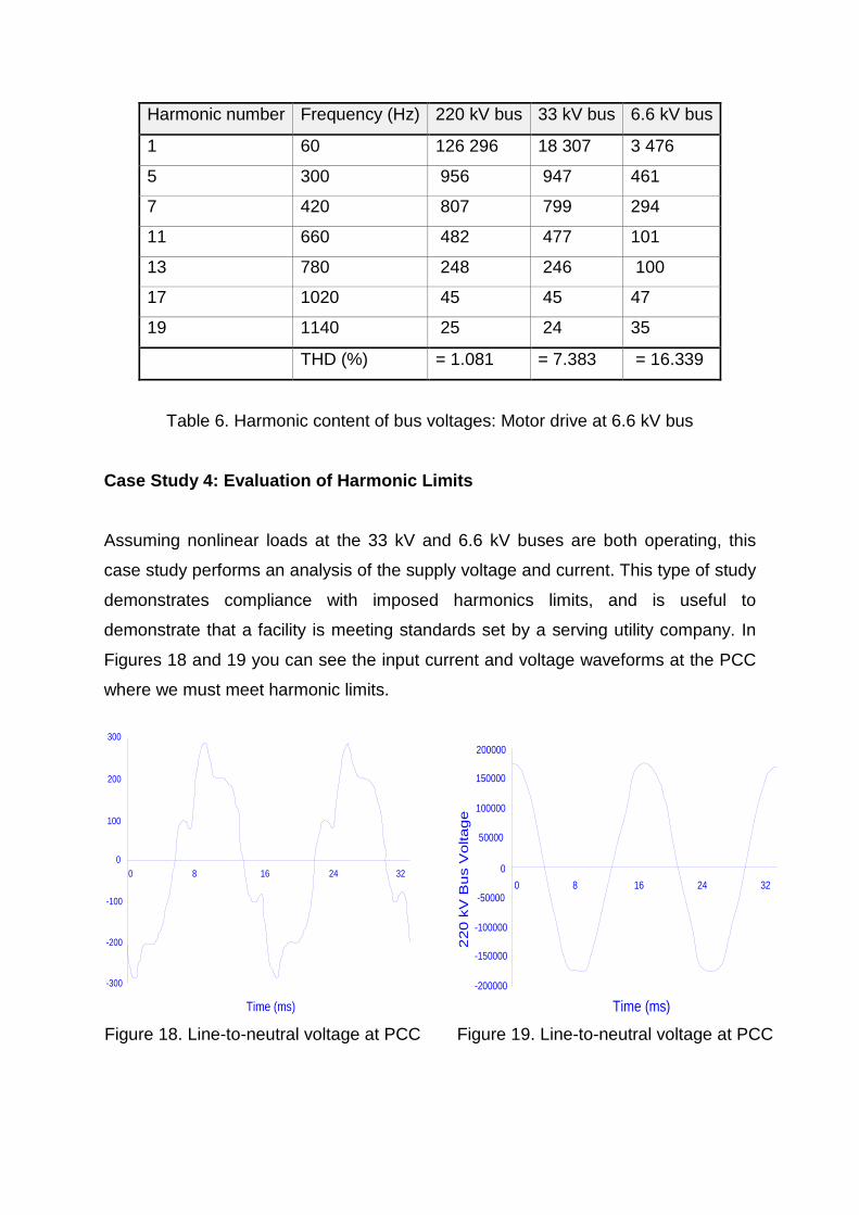
Case Study 4: Evaluation of Harmonic Limits

Assuming nonlinear loads at the 33 kV and 6.6 kV buses are both operating, this

case study performs an analysis of the supply voltage and current. This type of study

demonstrates compliance with imposed harmonics limits, and is useful to

demonstrate that a facility is meeting standards set by a serving utility company. In

Figures 18 and 19 you can see the input current and voltage waveforms at the PCC

where we must meet harmonic limits.

0

100

200

300

-100

-200

-300

0 8 16 24 32

Time (ms)

Figure 18. Line-to-neutral voltage at PCC Time (ms)

80 16 24 320

50000

100000

150000

200000

-50000

-100000

-150000

-200000

220

kV

Bu

s V

olta

ge

Figure 19. Line-to-neutral voltage at PCC

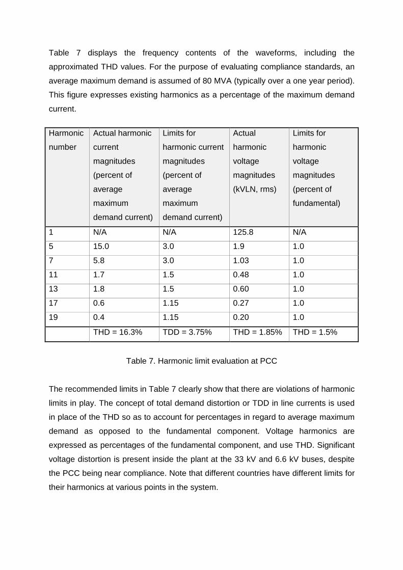
Table 7 displays the frequency contents of the waveforms, including the

approximated THD values. For the purpose of evaluating compliance standards, an

average maximum demand is assumed of 80 MVA (typically over a one year period).

This figure expresses existing harmonics as a percentage of the maximum demand

current.

Harmonic

number

Actual harmonic

current

magnitudes

(percent of

average

maximum

demand current)

Limits for

harmonic current

magnitudes

(percent of

average

maximum

demand current)

Actual

harmonic

voltage

magnitudes

(kVLN, rms)

Limits for

harmonic

voltage

magnitudes

(percent of

fundamental)

1 N/A N/A 125.8 N/A

5 15.0 3.0 1.9 1.0

7 5.8 3.0 1.03 1.0

11 1.7 1.5 0.48 1.0

13 1.8 1.5 0.60 1.0

17 0.6 1.15 0.27 1.0

19 0.4 1.15 0.20 1.0

THD = 16.3% TDD = 3.75% THD = 1.85% THD = 1.5%

Table 7. Harmonic limit evaluation at PCC

The recommended limits in Table 7 clearly show that there are violations of harmonic

limits in play. The concept of total demand distortion or TDD in line currents is used

in place of the THD so as to account for percentages in regard to average maximum

demand as opposed to the fundamental component. Voltage harmonics are

expressed as percentages of the fundamental component, and use THD. Significant

voltage distortion is present inside the plant at the 33 kV and 6.6 kV buses, despite

the PCC being near compliance. Note that different countries have different limits for

their harmonics at various points in the system.

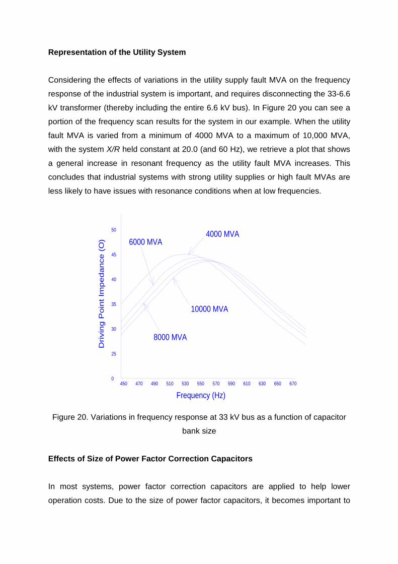
Representation of the Utility System

Considering the effects of variations in the utility supply fault MVA on the frequency

response of the industrial system is important, and requires disconnecting the 33-6.6

kV transformer (thereby including the entire 6.6 kV bus). In Figure 20 you can see a

portion of the frequency scan results for the system in our example. When the utility

fault MVA is varied from a minimum of 4000 MVA to a maximum of 10,000 MVA,

with the system X/R held constant at 20.0 (and 60 Hz), we retrieve a plot that shows

a general increase in resonant frequency as the utility fault MVA increases. This

concludes that industrial systems with strong utility supplies or high fault MVAs are

less likely to have issues with resonance conditions when at low frequencies.

Frequency (Hz)450 470 490 510 530 550 570 590 610 630 650 670

Driv

ing

Poi

nt Im

peda

nce

(O)

0

25

30

35

40

45

50 4000 MVA

10000 MVA

8000 MVA

6000 MVA

Figure 20. Variations in frequency response at 33 kV bus as a function of capacitor

bank size

Effects of Size of Power Factor Correction Capacitors

In most systems, power factor correction capacitors are applied to help lower

operation costs. Due to the size of power factor capacitors, it becomes important to

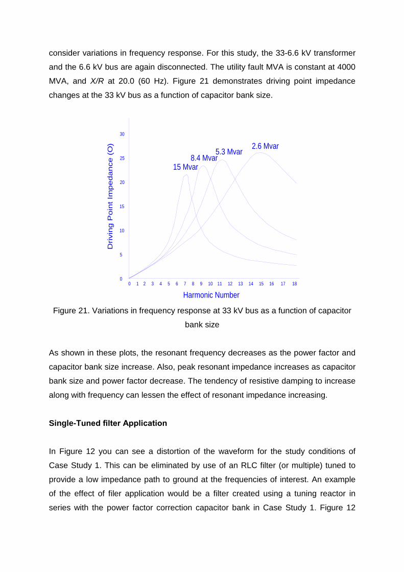
consider variations in frequency response. For this study, the 33-6.6 kV transformer

and the 6.6 kV bus are again disconnected. The utility fault MVA is constant at 4000

MVA, and X/R at 20.0 (60 Hz). Figure 21 demonstrates driving point impedance

changes at the 33 kV bus as a function of capacitor bank size.

Harmonic Number0 1 2 3 4 5 6 7 8 9 10 11 12 13 14 15 16 17 18

Driv

ing

Poi

nt Im

peda

nce

(O)

0

5

10

15

20

25

30

15 Mvar8.4 Mvar

5.3 Mvar 2.6 Mvar

Figure 21. Variations in frequency response at 33 kV bus as a function of capacitor

bank size

As shown in these plots, the resonant frequency decreases as the power factor and

capacitor bank size increase. Also, peak resonant impedance increases as capacitor

bank size and power factor decrease. The tendency of resistive damping to increase

along with frequency can lessen the effect of resonant impedance increasing.

Single-Tuned filter Application

In Figure 12 you can see a distortion of the waveform for the study conditions of

Case Study 1. This can be eliminated by use of an RLC filter (or multiple) tuned to

provide a low impedance path to ground at the frequencies of interest. An example

of the effect of filer application would be a filter created using a tuning reactor in

series with the power factor correction capacitor bank in Case Study 1. Figure 12

shows us via frequency scan results that the resonant point is near 480 Hz or the 8th

harmonic. The filter can be tuned to remove this resonance, however this more than

likely would produce a lower frequency resonance that coincides more with the

rectifier harmonics. Filter tuning frequencies should therefore be selected by

removing specific harmonic currents before they can excite resonant modes, instead

of selecting a tuning frequency to modify a specific frequency response. It is

important to apply a filter at the lowest current harmonic frequency, in this case 300

Hz or the 5th harmonic as mentioned above, as the application of single-tuned filters

tends to produce a new resonant point at a lower frequency. Ideally, a filter should

be tuned to this low frequency (i.e. 300 Hz) but often significant variations in system

parameters are enough to shift the resonant frequency in Figure 20 slightly. To

counter this, single-tuned filters can be, and often are, constructed based around a

target frequency 3-5% lower than that of the harmonic current to be removed.

Most applications use a single-tuned filter created from the existing power factor

correction capacitors. At power frequencies of 50-60 Hz, the series RLC combination

supplies reactive power to the system as it appears to be capacitive. The series

impedance at the tuned frequency is very low, and provides a low impedance path to

ground for the specific harmonic currents needed.

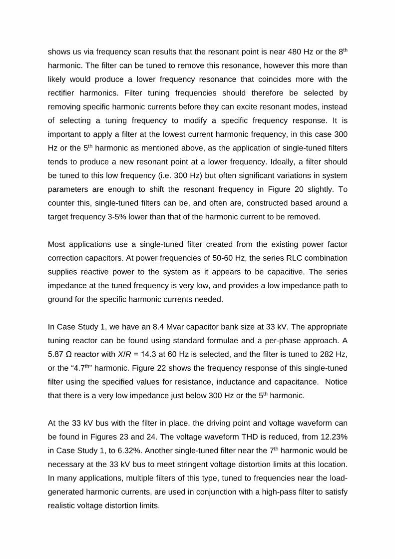
In Case Study 1, we have an 8.4 Mvar capacitor bank size at 33 kV. The appropriate

tuning reactor can be found using standard formulae and a per-phase approach. A

5.87 Ω reactor with X/R = 14.3 at 60 Hz is selected, and the filter is tuned to 282 Hz,

or the “4.7th” harmonic. Figure 22 shows the frequency response of this single-tuned

filter using the specified values for resistance, inductance and capacitance. Notice

that there is a very low impedance just below 300 Hz or the 5th harmonic.

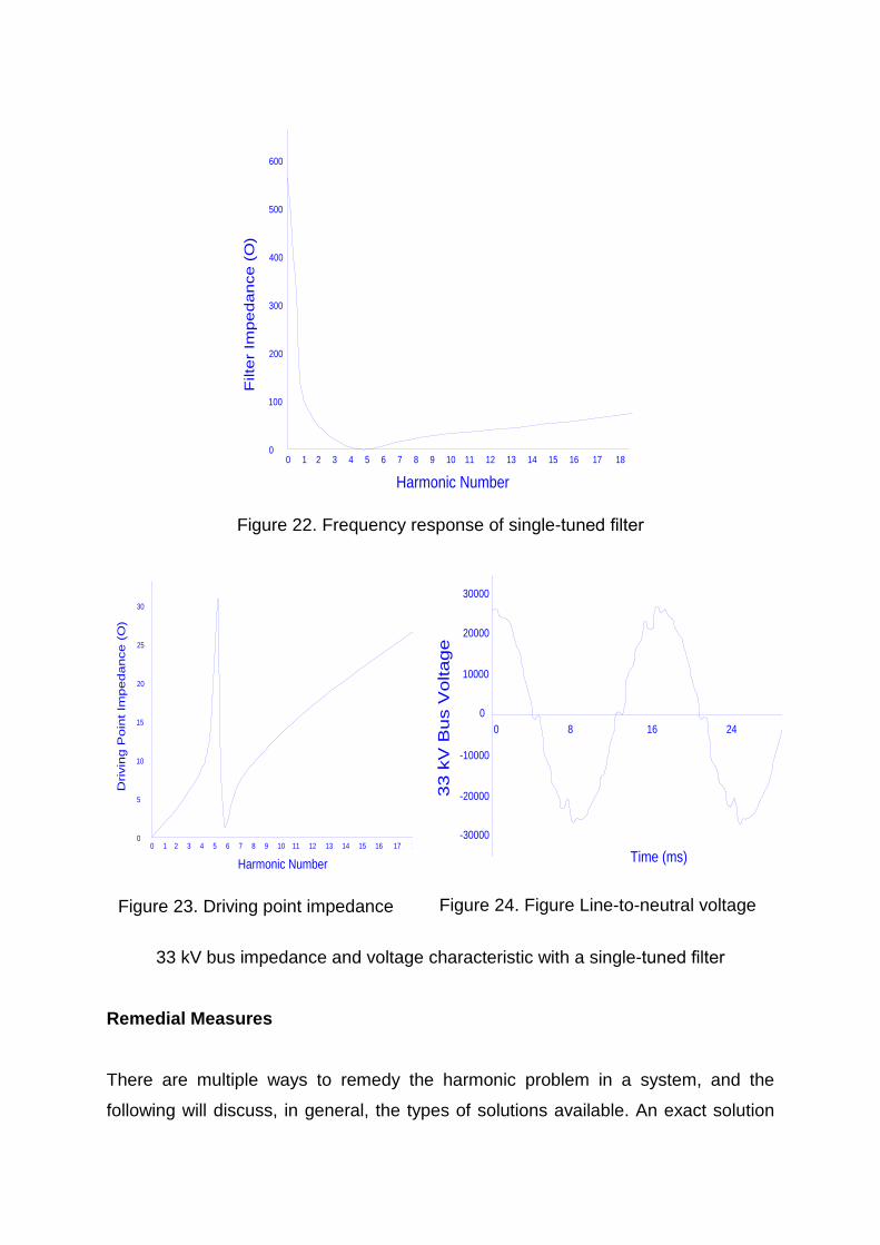
At the 33 kV bus with the filter in place, the driving point and voltage waveform can

be found in Figures 23 and 24. The voltage waveform THD is reduced, from 12.23%

in Case Study 1, to 6.32%. Another single-tuned filter near the 7th harmonic would be

necessary at the 33 kV bus to meet stringent voltage distortion limits at this location.

In many applications, multiple filters of this type, tuned to frequencies near the load-

generated harmonic currents, are used in conjunction with a high-pass filter to satisfy

realistic voltage distortion limits.

Harmonic Number0 1 2 3 4 5 6 7 8 9 10 11 12 13 14 15 16 17 18

Filt

er Im

peda

nce

(O)

0

100

200

300

400

500

600

Figure 22. Frequency response of single-tuned filter

Harmonic Number0 1 2 3 4 5 6 7 8 9 10 11 12 13 14 15 16 17 1

Driv

ing

Poi

nt Im

peda

nce

(O)

0

5

10

15

20

25

30

Figure 23. Driving point impedance

0

10000

20000

30000

-10000

-20000

-30000

0 8 16 24

Time (ms)

33 k

V B

us V

olta

ge

Figure 24. Figure Line-to-neutral voltage

33 kV bus impedance and voltage characteristic with a single-tuned filter

Remedial Measures

There are multiple ways to remedy the harmonic problem in a system, and the

following will discuss, in general, the types of solutions available. An exact solution

will depend on multiple factors, including whether the system is new or previously

existing, is flexible to changes, is open to adding harmonic filters, or is receptive to

modification of existing capacitor banks.

- Care should be taken when designing or expanding a system to ensure that

the total harmonic load is kept to a low percentage of the total plant load, with

around 30% being a good maximum target. Consideration should be given to

the location of harmonic loads, number of buses, size of transformers, choice

of connections, etc. in addition to adding harmonic filters, if the measured or

calculated levels of distortion are quite high.

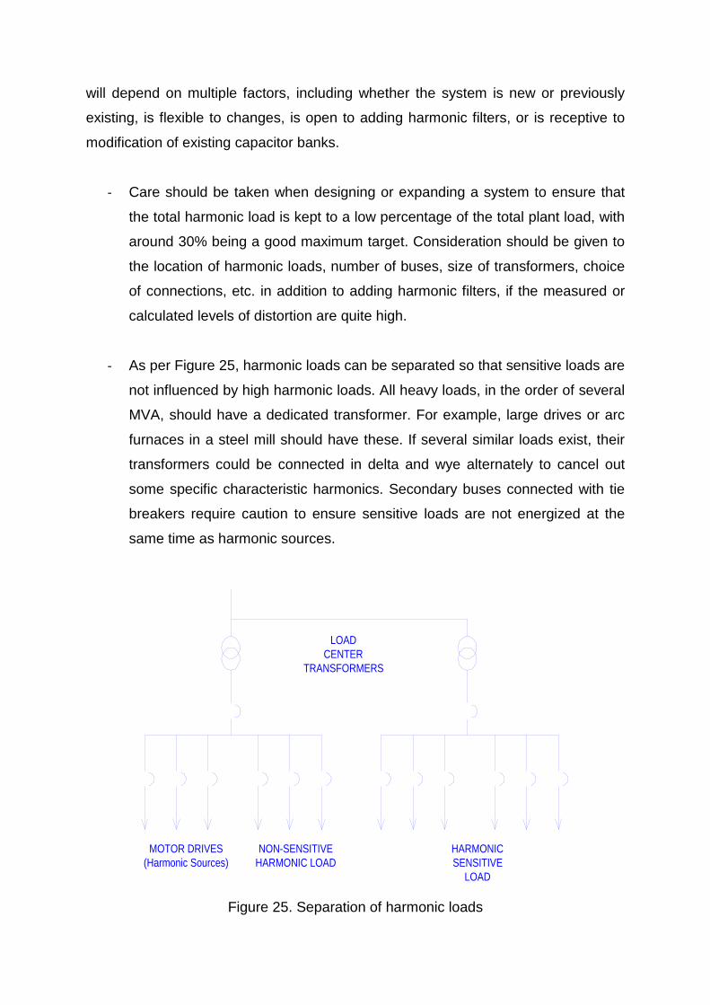
- As per Figure 25, harmonic loads can be separated so that sensitive loads are

not influenced by high harmonic loads. All heavy loads, in the order of several

MVA, should have a dedicated transformer. For example, large drives or arc

furnaces in a steel mill should have these. If several similar loads exist, their

transformers could be connected in delta and wye alternately to cancel out

some specific characteristic harmonics. Secondary buses connected with tie

breakers require caution to ensure sensitive loads are not energized at the

same time as harmonic sources.

NON-SENSITIVEHARMONIC LOAD

MOTOR DRIVES(Harmonic Sources)

HARMONICSENSITIVE

LOAD

LOADCENTER

TRANSFORMERS

Figure 25. Separation of harmonic loads

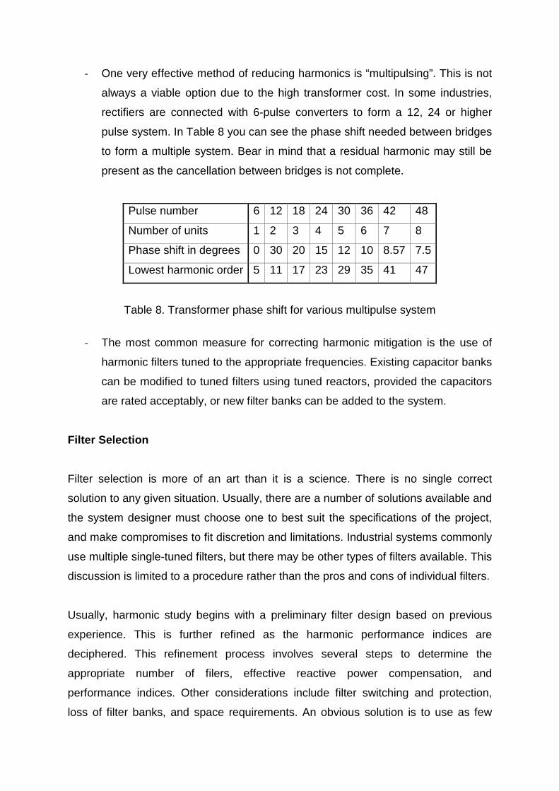
- One very effective method of reducing harmonics is “multipulsing”. This is not

always a viable option due to the high transformer cost. In some industries,

rectifiers are connected with 6-pulse converters to form a 12, 24 or higher

pulse system. In Table 8 you can see the phase shift needed between bridges

to form a multiple system. Bear in mind that a residual harmonic may still be

present as the cancellation between bridges is not complete.

Pulse number 6 12 18 24 30 36 42 48

Number of units 1 2 3 4 5 6 7 8

Phase shift in degrees 0 30 20 15 12 10 8.57 7.5

Lowest harmonic order 5 11 17 23 29 35 41 47

Table 8. Transformer phase shift for various multipulse system

- The most common measure for correcting harmonic mitigation is the use of

harmonic filters tuned to the appropriate frequencies. Existing capacitor banks

can be modified to tuned filters using tuned reactors, provided the capacitors

are rated acceptably, or new filter banks can be added to the system.

Filter Selection

Filter selection is more of an art than it is a science. There is no single correct

solution to any given situation. Usually, there are a number of solutions available and

the system designer must choose one to best suit the specifications of the project,

and make compromises to fit discretion and limitations. Industrial systems commonly

use multiple single-tuned filters, but there may be other types of filters available. This

discussion is limited to a procedure rather than the pros and cons of individual filters.

Usually, harmonic study begins with a preliminary filter design based on previous

experience. This is further refined as the harmonic performance indices are

deciphered. This refinement process involves several steps to determine the

appropriate number of filers, effective reactive power compensation, and

performance indices. Other considerations include filter switching and protection,

loss of filter banks, and space requirements. An obvious solution is to use as few

filters as possible, and compare this performance with no filter. Filter location is

something else to take into consideration. Effective filtering generally necessitates

that the filters be located at higher voltage levels, near the PCC or main bus, to meet

the demands of all harmonic sources.

Filters are most commonly tuned to one of the odd dominant characteristic

harmonics, starting from the lowest order. Generally this will be 5, 7, 11, etc. In some

cases the lowest order can be 2 or 3, as in arc furnace applications. Ideally filters

should be tuned to the exact harmonic order needed, but practical considerations

mean it may be necessary to tune below the nominal frequency. If the parallel

resonance frequency needs to be offset, the filter may intentionally be tuned above

or below the nominal frequency. For example, if a 5th harmonic filter causes

resonance near the 3rd, tuning it slightly below or above the 5th can offset the

resonance at the 3rd. Another example is where the resonant frequency is very close

to the 5th, e.g. 4.7 for very sharp filters, it will be desirable to tune it below to avoid

the resonant frequency coinciding with the harmonic injection frequency when

accounting for tolerances, temperature deviations, etc.

Capacitors and reactors, the two main parts of a passive filter, are discussed here.

The nominal fundamental kvar rating of capacitors determines the harmonic filtering

effectivity. An initial estimate of the capacitor kvar is therefore very important. A

larger bank size makes it easier to meet a given harmonic performance criteria.

Beside the harmonic requirements, you may need to consider the following design

factors:

- The system power factor or displacement power factor may be corrected to a

required or more desirable value, usually above 0.9.

- If a transformer is overloaded, the total kVA demand on the supply

transformer may have to be reduced.

- The current ratings of buses and cables may also have to be reduced.

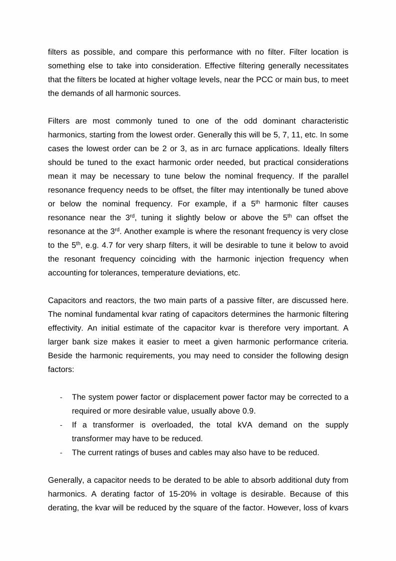
Generally, a capacitor needs to be derated to be able to absorb additional duty from

harmonics. A derating factor of 15-20% in voltage is desirable. Because of this

derating, the kvar will be reduced by the square of the factor. However, loss of kvars

is somewhat compensated for by the cancellation of capacitive reactance in the

filters inductive reactance. The effect of this is to increase the voltage of a capacitor

(above bus voltage) by the factor below.

𝑟𝑟 = ℎ2

ℎ2−1 Eq. (22)

For a conventional single-tuned filter this factor is calculated in Table 9.

Harmonic order 3rd 5th 7th 11th 13th

Per-unit voltage 1.125 1.049 1.021 1.008 1.005

Table 9. Fundamental voltage across a single-tuned filter capacitor

When the harmonic study is finished, and the filter selection is complete, a capacitor

rating with respect to voltage, current and kvar should be checked. These three

elements need to be individually satisfied. The filter designer can do this himself if

standard units are used, or the capacitor supplier can be requested to meet them if

special units are used.

In industrial applications, an air or iron core reactor can be used, depending on size

and cost. In general, iron-core reactors are limited to 13.8 kV, while air-core reactors

can cover the complete range of low, medium, and high voltage applications. Iron-

core reactors can save space and can be enclosed in housing either indoors or

outdoors, along with capacitors and other components as needed.

Reactors need to be rated for the maximum fundamental current along with the worst

generated harmonics for the “worst” system configuration. The reactor vendor must

calculate all losses, fundamental and harmonic, core in the case of iron-core

reactors, and stray due to frequency effects. This is to ensure hot-spot temperatures

are within acceptable limits for dielectric temperature.

A big unknown in the filter design is the Q factor, or the ratio of inductive resistance

to that of the tuned frequency. This can generally be estimated based on prior

experience, but if it is determined during the study that Q is not critical, the reactor

should be specified to have the “natural Q”, or that of the reactor that is naturally

obtained with no cost or design consideration. However, if a low-Q reactor will help

mitigate amplifications near parallel resonance, then a low-Q reactor should be

specified. Manufacturers have a high tolerance of up to 20% that should be

recognized in Q values. Bear in mind that a low-Q design will produce higher losses.