introduction to hidden markov models for gene...

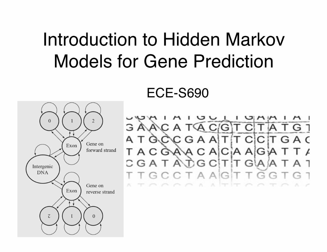
Introduction to Hidden Markov Models for Gene Prediction

ECE-S690

Outline

 Markov Models  The Hidden Part  How can we use this for gene

prediction?

Learning Models

 Want to recognize patterns (e.g. sequence motifs), we have to learn from the data

Markov Chains

A B C Probability

of Transition

Probability of

Transition

Current State only depends on previous state and transition

probability

aBA=Pr(xi=B|xi-1=A)

Example: Estimating Mood State from Grad Student Observations

Example: “Happy” Grad Student Markov Chain

Lab Coffee Shop Bar

0.5

0.3 0.2

0.2

0.7

0.2

Observations: Lab, Coffee, Lab, Coffee, Lab, Lab, Bar, Lab, Coffee,…

0.5

0.3

0.1

Depressed about research

Lab Coffee Shop Bar

0.05

0.1 0.75

0.8

0.1

0.2

0.1

0.2

0.7

Evaluating Observations

 The probability of observing a given sequence is equal to the product of all observed transition probabilities.

 P(Coffee->Bar->Lab) = P(Coffee) P(Bar | Coffee) P(Lab | Bar)

P(CBL) = P(L|B) P(B|C)P(C)

X are the observations

1st order model

 Probability of Next State | Previous State  Calculate all probabilities

Convert “Depressed” Observations to Matrix

Lab Coffee Shop Bar

0.05

0.1 0.75

0.8

0.1

0.2

0.1

0.2

0.7

Scoring Observations: Depressed Grad Student

From Lab

From Coffee Shop

From Bar

To Lab 0.1 0.05 0.2

To Coffee Shop

0.1 0.2 0.1

To Bar 0.8 0.75 0.7

Pr from each state add to 1

Student 1:LLLCBCLLBBLL Student 2:LCBLBBCBBBBL Student 3:CCLLLLCBCLLL


From Lab

From Coffee Shop

From Bar

To Lab 0.1 0.05 0.2

To Coffee Shop

0.1 0.2 0.1

To Bar 0.8 0.75 0.7

Student 1:LLLCBCLLBBLL


p’s


From Lab

From Coffee Shop

From Bar

To Lab 0.1 0.05 0.2

To Coffee Shop

0.1 0.2 0.1

To Bar 0.8 0.75 0.7

Student 1:LLLCBCLLBBLL



From Lab

From Coffee Shop

From Bar

To Lab 0.1 0.05 0.2

To Coffee Shop

0.1 0.2 0.1

To Bar 0.8 0.75 0.7

Student 1:LLLCBCLLBBLL = 4.2x10-9 Student 2:LCBLBBCBBBBL = 4.3x10-5 Student 3:CCLLLLCBCLLL = 3.8x10-11


p’s

Equilibrium State From Lab

From Coffee Shop

From Bar

To Lab 0.333 0.333 0.333

To Cofee Shop

0.333 0.333 0.333

To Bar 0.333 0.333 0.333

Student 1:LLLCBCLLBBLL = 5.6x10-6 Student 2:LCBLBBCBBBBL = 5.6x10-6 Student 3:CCCLCCCBCCCL = 5.6x10-6

q’s

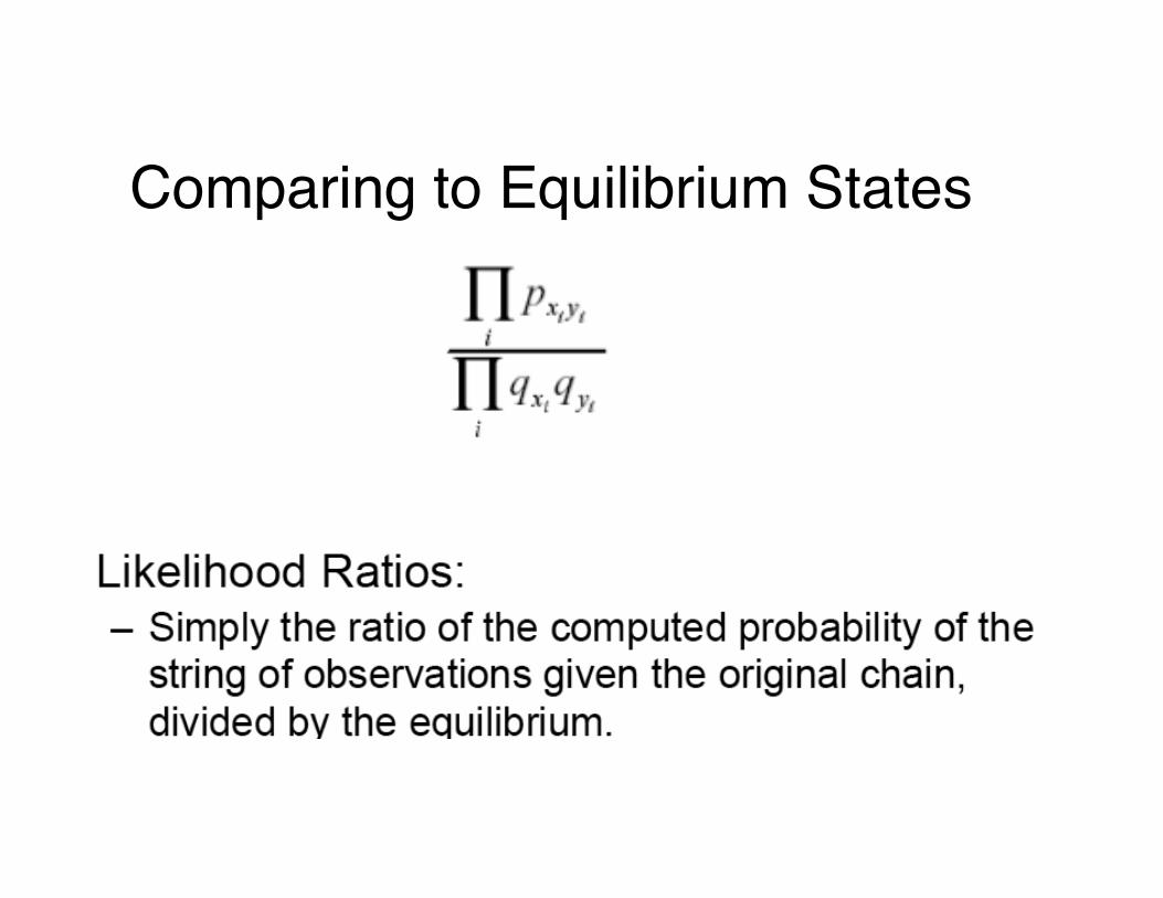
Comparing to Equilibrium States

Evaluation Observations

 Likelihood ratios:  Student 1 = 4.2x10-9 / 5.6x10-6 = 7.5x10-4  Student 2 = 4.3x10-5 / 5.6x10-6 = 7.7  Student 3 = 3.8x10-11 / 5.6x10-6 = 6.8 x 10-6

 Log likelihood ratios  Student 1 = -3.2  Student 2 = 0.9 (Most likely sad)  Student 3 = -5.2

The model could represent Research Breakthrough (Happy) Student!: Transition Probabilities

From Lab

From Coffee Shop

From Bar

To Lab 0.6 0.75 0.5

To Cofee Shop

0.25 0.2 0.45

To Bar 0.15 0.05 0.05

Combined Model

Lab Coffee Shop Bar

Lab Coffee Shop Bar

Happy Student

Depressed Student

“Generalized” HMM

Lab Coffee Shop Bar

Lab Coffee Shop Bar

Emission

Transition

Happy

Depressed

Generalized HMM - Combined Model

Lab Coffee Shop Bar

Lab Coffee Shop Bar

Start End

Happy

Depressed

Simplifying the Markov Chains to 0th order to model hidden states

 Happy: Lab: 75%, Coffee: 20%, Bar 5%  Sad: Lab:40%, Coffee: 20%, Bar 40%

HMM - Combined Model

Start End

Happy

Depressed

L: 0.75 C: 0.2 B: 0.05

L: 0.4 C: 0.2 B: 0.4

Hiddenness

Evaluating Hidden State

 Evaluating Hidden State  Observations: LLLCBCLLBBLLCBLBBCBBBBLCLLLCCL Hidden state: HHHHHHHHHHHHHDDDDDDDDDDHHHHHHH

Applications

Particulars about HMMs

Gene Prediction

Why are HMMs a good fit for DNA and Amino Acids?

HMM Caveats

•  States are supposed to be independent of each other and this isn’t always true • Need to be mindful of overfitting – Need a good training set – More training data does not always mean a better model • HMMs can be slow (if proper Decoding not implemented) – Some decoding maps out all paths through the model – DNA sequences can be very long so processing/ annotating them can be very time consuming

Genomic Applications

  Finding Genes   Finding Pathogenicity Islands

Neisseria meningitidis, 52% G+C

(from Tettelin et al. 2000. Science)

GC Content

Example Bio App: Pathogenicity Islands

 Clusters of genes acquired by horizontal transfer  Present in pathogenic species

but not others  Frequently encode virulence

factors  Toxins, secondary

metabolites, adhesins

 (Flanked by repeats, regulation and have different codon usage)

 Different GC content than rest of genome

Modeling Sequence Composition (Simple Probability of Sequence)

  Calculate sequence distribution from known islands   Count occurrences of A,T,G,C

  Model islands as nucleotides drawn independently from this distribution

A: 0.15 T: 0.13 G: 0.30 C: 0.42

… … A: 0.15 T: 0.13 G: 0.30 C: 0.42

A: 0.15 T: 0.13 G: 0.30 C: 0.42

P(Si|MP)

... C C TA A G T T A G A G G A T T G A G A ….

The Probability of a Sequence (Simplistic)

 Can calculate the probability of a particular sequence (S) according to the pathogenicity island model (MP)

Example

S = AAATGCGCATTTCGAA A: 0.15 T: 0.13 G: 0.30 C: 0.42

Background Island

0.15

0.25 0.75 0.85

A: 0.25 T: 0.25 G: 0.25 C: 0.25

TAAGAATTGTGTCACACACATAAAAACCCTAAGTTAGAGGATTGAGATTGGCA GACGATTGTTCGTGATAATAAACAAGGGGGGCATAGATCAGGCTCATATTGGC

A: 0.15 T: 0.13 G: 0.30 C: 0.42

A More Complex Model

P

B B

P P

B

P P

B

P

B

P

B

P

B

P

B

A Generative Model

P P

B B B

P P

C A A A T G C G S:

B B B

P P P

B B

A: 0.42 T: 0.30 G: 0.13 C: 0.15

A: 0.25 T: 0.25 G: 0.25 C: 0.25

P(S|P) P(S|B) P(Li+1|Li) Bi+1 Pi+1

Bi 0.85 0.15

Pi 0.25 0.75

The Hidden in HMM

 DNA does not come conveniently labeled (i.e. Island, Gene, Promoter)

 We observe nucleotide sequences

  The hidden in HMM refers to the fact that state labels, L, are not observed  Only observe emissions (e.g.

nucleotide sequence in our example)

State i State j

…A A G T T A G A G…

A Hidden Markov Model

Hidden States L = { 1, ..., K }

Transition probabilities akl = Transition probability from state k to state l

Emission probabilities ek(b) = P( emitting b | state=k)

Initial state probability π(b) = P(first state=b)

State i State j

el(b) ek(b)

Emission Probabilities

Transition Probabilities

HMM with Emission Parameters

 a13: Probability of a transition from State 1 to State 3

 e2(A): Probability of emitting character A in state 2

Hidden Markov Models (HMM)

 Allows you to find sub-sequence that fit your model

 Hidden states are disconnected from observed states

 Emission/Transition probabilities  Must search for optimal paths

Three Basic Problems of HMMs  The Evaluation Problem

 Given an HMM and a sequence of observations, what is the probability that the observations are generated by the model?

 The Decoding Problem  Given a model and a sequence of observations, what

is the most likely state sequence in the model that produced the observations?

 The Learning Problem  Given a model and a sequence of observations, how

should we adjust the model parameters in order to maximize evaluation/decoding

Fundamental HMM Operations

Decoding   Given an HMM and sequence S   Find a corresponding sequence

of labels, L Evaluation   Given an HMM and sequence S   Find P(S|HMM)

Training   Given an HMM w/o parameters

and set of sequences S   Find transition and emission

probabilities the maximize P(S | params, HMM)

Computation Biology

Annotate pathogenicity islands on a new sequence

Score a particular sequence

Learn a model for sequence composed of background DNA and pathogenicity islands

Markov chains and processes 1st order Markov chain

2nd order Markov chain

1st order with stochastic observations -- HMM

HMM - Combined Model for Gene Detection

Start End

Coding

Noncoding

1st-order transition matrix (4x4)

A C G T

A 0.2 0.15 0.25 0.2

C 0.3 0.35 0.25 0.2

G 0.3 0.4 0.3 0.3

T 0.2 0.1 0.2 0.2

2nd Order Model (16x4)

A C G T AA 0.1 0.3 0.25 0.05 AC 0.05 0.25 0.3 0.1 AG 0.3 0.05 0.1 0.25 AT 0.25 0.1 0.05 0.3

.

.

.

Three Basic Problems of HMMs

 The Evaluation Problem  Given an HMM and a sequence of observations, what

is the probability that the observations are generated by the model?

 The Decoding Problem  Given a model and a sequence of observations, what

is the most likely state sequence in the model that produced the observations?

 The Learning Problem  Given a model and a sequence of observations, how

should we adjust the model parameters in order to maximize

What Questions can an HMM Answer?

Viterbi Algorithm: What is the most probable path that generated sequence X? Forward Algorithm: What is the likelihood of sequence X given HMM M – Pr(X|M)? Forward-Backward (Baum-Welch) Algorithm: What is the probability of a particular state k having generated symbol Xi?

“Decoding” With HMM

Pathogenicity Island Example Given a nucleotide sequence, we want a labeling of each nucleotide as either “pathogenicity island” or “background DNA”

Given observations, we would like to predict a sequence of hidden states that is most likely to have generated that sequence

The Most Likely Path

 Given observations, one reasonable choice for labeling the hidden states is:

The sequence of hidden state labels, L*, (or path) that makes the labels and

sequence most likely given the model

Probability of a Path,Seq

P

B

P

B

P

B B

P

B B

P

B

P

B

G C A A A T G C

L:

S:

P P

0.25 0.25

B B B

0.25

0.85 0.85 0.85 0.85 B B B B B

0.85

0.25

0.85

0.25 0.25 0.25 0.25

0.85

Probability of a Path,Seq

P

B

P

B

P

B B

P

B B

P

B

P

B

G C A A A T G C

L:

S:

P P

B B B B B 0.85

0.25

0.85

0.15 0.25

0.25 0.25 0.42 0.42 0.30 0.25 0.25

0.85

P P P 0.75 0.75

We could try to calculate the probability of every path, but….

Decoding

 Viterbi Algorithm  Finds most likely sequence of hidden states or

labels, L* or P* or π*, given sequence and model

 Uses dynamic programming (same technique used in sequence alignment)

 Much more efficient than searching every path

Finding Best Path

 Viterbi  Dynamic programming  Maximize Probability Emission of

observations on trace-back

Viterbi Algorithm

Most probable state path given sequence (observations)?

Viterbi (in pseudocode)

 l is previous state and k is next state  vl(i)= el(xi) maxk(vk(i-1)akl)  π* are the paths that maximizes the

probability of the previous path times new transition in maxk(vk(i-1)akl)

Each node picks one max Start

Forward Alg: Probability of a Single Label (Hidden State)

 Calculate most probable label, L*i , at each position i

 Do this for all N positions gives us {L*1, L*

2, L*3…. L*

N}

P

B

P

B

P

B B

P

B B

P

B

P

B

G C A A A T G C

L:

S:

P P P

B

P

B

P

B B

P

B B

P

B

P

B

P P Sum over all paths

P(Label5=B|S) Forward algorithm (dynamic programming)

fl(i) = el(xi) Σkfk(i-1)akl

Forward Algorithm

Start

fl(i) = el(xi) Σkfk(i-1)akl

P(x) = Σk fk(N)ak0

Add probs of all Different paths to get Probability of sequence

 Viterbi Algorithm  Finds most likely sequence of hidden states, L* or P*

or π*, given sequence and model

 Posterior Decoding  Finds most likely label at each position for all

positions, given sequence and model {L*

1, L*2, L*

3…. L*N}

 Forward and Backward equations

Two Decoding Options

Relation between Viterbi and Forward VITERBI

Vj(i) = P(most probable path ending in state j with observation i )

Initialization: V0(0) = 1 Vk(0) = 0, for all k > 0

Iteration: Vl(i)= el(xi)maxkVk(i-1) akl

Termination: P(x, π*) = maxkVk(N)

FORWARD

fl(i)=P(x1…xi,statei=l)

Initialization: f0(0) = 1 fk(0) = 0, for all k > 0

Iteration: fl(i) = el(xi) Σkfk(i-1)akl

Termination: P(x) = Σk fk(N)ak0

Forward/Backward Algorithms

 Way to compute probability of most probable path

 Forward and Backward can be combined to find Probability of emission, xi from state k given sequence x. P(πi=k | x)

 P(πi=k | x) is called posterior decoding  P(πi=k | x) = fk(I)bk(I)/P(x)

Example Application: Bacillus subtilis

Method

Nicolas et al (2002) NAR

Gene+ Gene-

AT Rich

Second Order Emissions

P(Si)=P(Si|State,Si-1,Si-2) (capturing trinucleotide

Frequencies)

Train using EM

Predict w/Posterior Decoding

Three State Model

Results

Nicolas et al (2002) NAR

Gene on positive strand

Each line is P(label|S,model)

color coded by label

Gene on negative strand

A/T Rich -  Intergenic regions -  Islands

Training an HMM

Transition probabilities e.g. P(Pi+1|Bi) – the probability of entering a pathogenicity island from background DNA

Emission probabilities i.e. the nucleotide frequencies for background DNA and pathogenicity islands

B P

P(S|P) P(S|B)

P(Li+1|Li)

Learning From Labelled Data

P

B

P

B

P

B B

P

B B

P

B

P

B

G C A A A T G C

L:

S:

If we have a sequence that has islands marked, we can simply count

A: T: G: C:

P(S|P) P(S|B) P(Li+1|Li) Bi+1 Pi+1 End

Bi 3/5 1/5 1/5

Pi 1/3 2/3 0

Start 1 0 0

End start

P

B B B B B

P

ETC.. ! A: 1/5

T: 0 G: 2/5 C: 2/5

Unlabelled Data

P

B

P

B

P

B B

P

B B

P

B

P

B

G C A A A T G C

L:

S:

How do we know how to count?

A: T: G: C:

A: T: G: C:

P(S|P) P(S|B) P(Li+1|Li)

Start

? Pi

Pi+1

Bi

End Bi+1

End start

P P

?

Unlabeled Data

An idea: 1. Imagine we start with some parameters

(e.g. initial or bad model)

2. We could calculate the most likely path, P*, given those parameters and S

3. We could then use P* to recalculate our parameters by maximum likelihood

4. And iterate (to convergence)

P

B

P

B

P

B B

P

B B

P

B

P

B

G C A A A T G C

L:

S:

P(S|P)0 P(S|B)0 P(Li+1|Li)0

End start

P P



P(S|P)K P(S|B)K P(Li+1|Li)K

…

B B B B B B B B B B B B B

P P P

Training Models for Classification

 Correct Order for the model  Higher order models remember more “history”   Additional history can have predictive value

  Example:   predict the next word in this sentence fragment   “…finish __” (up, it, first, last, …?)   now predict it given more history   “Fast guys finish __”

Model Order  However, the number of parameters to estimate

grows exponentially with the order for modeling DNA we need parameters for an nth order model, with n>=5 normally

 The higher the order, the less reliable we can expect our parameter estimates to be   estimating the parameters of a 2nd order Markov

chain from the complete genome of E. Coli, each word > 72,000 times on average

  estimating the parameters of an 8th order chain, word 5 times on average

HMMs in Context

  HMMs   Sequence alignment  Gene Prediction

  Generalized HMMs   Variable length states   Complex emissions models   e.g. Genscan

  Bayesian Networks  General graphical model   Arbitrary graph structure   e.g. Regulatory network

analysis

HMMs can model different regions

Example Model for Gene Recognition

Promoter C Start Trans- cription Factor

Exon Splice Intron

Repeat

End

Another Example

CpG Islands: Another Application

 CG dinucleotides are rarer in eukaryotic genomes than expected given the independent probabilities of C, G

 Particularly, the regions upstream of genes are richer in CG dinucleotides than elsewhere - CpG islands

Most transitions omitted for clarity

A+ C+

G+ T+

+aGC +aCG

A- C-

G- T-

-aGC -aCG B E

-+aAC

CpG island DNA states: large C, G transition

probabilities

“Normal DNA” states: small C, G transition

probabilities

CpG Island Sub-model Normal DNA Sub-model

CpG Islands

CpG Islands

  In human genome, CG dinucleotides are relatively rare  CG pairs undergo a process called methylation

that modifies the C nucleotide  A methylated C mutate (with relatively high

chance) to a T  Promotor regions are CG rich

 These regions are not methylated, and thus mutate less often

 These are called CG (aka CpG) islands

CpG Island Prediction

  In a CpG island, the probability of a “C” following a “G” is much higher than in “normal” intragenic DNA sequence.

 We can construct an HMM to model this by combining two HMMs: one for normal sequence and one for CpG island sequence.

  Transitions between the two sub-models allow the model to switch between CpG island and normal DNA.

  Because there is more than one state that can generate a given character, the states are “hidden” when you just see the sequence.

  For example, a “C” can be generated by either the C+ or C-

states in the following model.

Inhomogenous Markov Chains Borodovsky’s Lab: http://exon.gatech.edu/GeneMark/

Variable-length

Full

Variable Length

Interpolated HMMs

 Manage Model Trade-off by interpolating between various HMM Model orders

 GlimmerHMM

The Three Basic HMM Problems

  Problem 1 (Evaluation): Given the observation sequence O=o1,…,oT and an

HMM model, how do we compute the probability of O given the model?

  Problem 2 (Decoding): Given the observation sequence O=o1,…,oT and an

HMM model, how do we find the state sequence that best explains the observations?

 Problem 3 (Learning): How do we adjust the model parameters to maximize the probability of observations given the model?

The Three Basic HMM Problems

Conclusions

 Markov Models  HMMs  Issues  Applications

Example of Viterbi, Forward, Backward, and Posterior Algorithms

Real DNA sequences are inhomogeneous and can be described by a hidden Markov model with hidden states representing different types of nucleotide composition. Consider an HMM that includes two hidden states H and L for high and lower C+G content, respectively. Initial probabilities for both H and L are equal to 0.5, while transition probabilities are as follows: aHH=0.5, aHL=0.5, aLL=0.6, aLH=0.4. Nucleotides T, C, A, G are emitted from states H and L with probabilities 0.2, 0.3, 0.2, 0.3, and 0.3, 0.2, 0.3, 0.2, respectively. Use the Viterbi algorithm to define the most likely sequence of hidden states for the sequence, X=TGC.

introduction to hidden markov models for gene...

Documents