introduction to lie groups - alistair...
TRANSCRIPT
Introduction to Lie GroupsMAT 4144/5158
Winter 2015
Alistair Savage
Department of Mathematics and Statistics
University of Ottawa
This work is licensed under aCreative Commons Attribution-ShareAlike 4.0 International License
Contents
Preface iii
1 Introduction and first examples 11.1 Category theoretic definitions . . . . . . . . . . . . . . . . . . . . . . . . . . 11.2 The circle: S1 . . . . . . . . . . . . . . . . . . . . . . . . . . . . . . . . . . . 31.3 Matrix representations of complex numbers . . . . . . . . . . . . . . . . . . . 51.4 Quaternions . . . . . . . . . . . . . . . . . . . . . . . . . . . . . . . . . . . . 61.5 Quaternions and space rotations . . . . . . . . . . . . . . . . . . . . . . . . . 91.6 Isometries of Rn and reflections . . . . . . . . . . . . . . . . . . . . . . . . . 141.7 Quaternions and rotations of R4 . . . . . . . . . . . . . . . . . . . . . . . . . 161.8 SU(2)× SU(2) and SO(4) . . . . . . . . . . . . . . . . . . . . . . . . . . . . 17
2 Matrix Lie groups 202.1 Definitions . . . . . . . . . . . . . . . . . . . . . . . . . . . . . . . . . . . . . 202.2 Finite groups . . . . . . . . . . . . . . . . . . . . . . . . . . . . . . . . . . . 212.3 The general and special linear groups . . . . . . . . . . . . . . . . . . . . . . 212.4 The orthogonal and special orthogonal groups . . . . . . . . . . . . . . . . . 212.5 The unitary and special unitary groups . . . . . . . . . . . . . . . . . . . . . 222.6 The complex orthogonal groups . . . . . . . . . . . . . . . . . . . . . . . . . 232.7 The symplectic groups . . . . . . . . . . . . . . . . . . . . . . . . . . . . . . 232.8 The Heisenberg group . . . . . . . . . . . . . . . . . . . . . . . . . . . . . . 252.9 The groups R∗, C∗, S1 and Rn . . . . . . . . . . . . . . . . . . . . . . . . . . 262.10 The Euclidean group . . . . . . . . . . . . . . . . . . . . . . . . . . . . . . . 262.11 Homomorphisms of Lie groups . . . . . . . . . . . . . . . . . . . . . . . . . . 27
3 Topology of Lie groups 293.1 Connectedness . . . . . . . . . . . . . . . . . . . . . . . . . . . . . . . . . . . 293.2 Polar Decompositions . . . . . . . . . . . . . . . . . . . . . . . . . . . . . . . 333.3 Compactness . . . . . . . . . . . . . . . . . . . . . . . . . . . . . . . . . . . 363.4 Lie groups . . . . . . . . . . . . . . . . . . . . . . . . . . . . . . . . . . . . . 37
4 Maximal tori and centres 394.1 Maximal tori . . . . . . . . . . . . . . . . . . . . . . . . . . . . . . . . . . . 394.2 Centres . . . . . . . . . . . . . . . . . . . . . . . . . . . . . . . . . . . . . . 444.3 Discrete subgroups and the centre . . . . . . . . . . . . . . . . . . . . . . . . 45
i
ii CONTENTS
5 Lie algebras and the exponential map 475.1 The exponential map onto SO(2) . . . . . . . . . . . . . . . . . . . . . . . . 475.2 The exponential map onto SU(2) . . . . . . . . . . . . . . . . . . . . . . . . 485.3 The tangent space of SU(2) . . . . . . . . . . . . . . . . . . . . . . . . . . . 495.4 The Lie algebra su(2) of SU(2) . . . . . . . . . . . . . . . . . . . . . . . . . 515.5 The exponential of square matrices . . . . . . . . . . . . . . . . . . . . . . . 525.6 The tangent space . . . . . . . . . . . . . . . . . . . . . . . . . . . . . . . . 555.7 The tangent space as a Lie algebra . . . . . . . . . . . . . . . . . . . . . . . 595.8 Complex Lie groups and complexification . . . . . . . . . . . . . . . . . . . . 615.9 The matrix logarithm . . . . . . . . . . . . . . . . . . . . . . . . . . . . . . . 645.10 The exponential mapping . . . . . . . . . . . . . . . . . . . . . . . . . . . . 655.11 The logarithm into the tangent space . . . . . . . . . . . . . . . . . . . . . . 675.12 Some more properties of the exponential . . . . . . . . . . . . . . . . . . . . 715.13 The functor from Lie groups to Lie algebras . . . . . . . . . . . . . . . . . . 735.14 Lie algebras and normal subgroups . . . . . . . . . . . . . . . . . . . . . . . 785.15 The Campbell–Baker–Hausdorff Theorem . . . . . . . . . . . . . . . . . . . . 79
6 Covering groups 856.1 Simple connectedness . . . . . . . . . . . . . . . . . . . . . . . . . . . . . . . 856.2 Simply connected Lie groups . . . . . . . . . . . . . . . . . . . . . . . . . . . 886.3 Three Lie groups with tangent space R . . . . . . . . . . . . . . . . . . . . . 896.4 Three Lie groups with the cross-product Lie algebra . . . . . . . . . . . . . . 906.5 The Lie group-Lie algebra correspondence . . . . . . . . . . . . . . . . . . . 916.6 Covering groups . . . . . . . . . . . . . . . . . . . . . . . . . . . . . . . . . . 956.7 Subgroups and subalgebras . . . . . . . . . . . . . . . . . . . . . . . . . . . . 97
7 Further directions of study 1017.1 Lie groups, Lie algebras, and quantum groups . . . . . . . . . . . . . . . . . 1017.2 Superalgebras and supergroups . . . . . . . . . . . . . . . . . . . . . . . . . 1017.3 Algebraic groups and group schemes . . . . . . . . . . . . . . . . . . . . . . 1027.4 Finite simple groups . . . . . . . . . . . . . . . . . . . . . . . . . . . . . . . 1027.5 Representation theory . . . . . . . . . . . . . . . . . . . . . . . . . . . . . . 103
Preface
These are notes for the course Introduction to Lie Groups (cross-listed as MAT 4144 andMAT 5158) at the University of Ottawa. At the title suggests, this is a first course in thetheory of Lie groups. Students are expected to a have an undergraduate level backgroundin group theory, ring theory and analysis. We focus on the so-called matrix Lie groups sincethis allows us to cover the most common examples of Lie groups in the most direct mannerand with the minimum amount of background knowledge. We mention the more generalconcept of a general Lie group, but do not spend much time working in this generality.
After some motivating examples involving quaternions, rotations and reflections, we givethe definition of a matrix Lie group and discuss the most well-studied examples, includingthe classical Lie groups. We then study the topology of Lie groups, their maximal tori,and their centres. In the second half of the course, we turn our attention to the connectionbetween Lie algebras and Lie groups. We conclude with a discussion of simply connectedLie groups and covering groups.
Acknowledgement: The author would like to thank the students of MAT 4144/5158 formaking this such an enjoyable course to teach, for asking great questions, and for pointingout typographical errors in the notes.
Alistair Savage Ottawa, 2015.
Course website: http://alistairsavage.ca/mat4144/
iii
Chapter 1
Introduction and first examples
In this chapter we introduce the concept of a Lie group and then discuss some importantbasic examples.
1.1 Category theoretic definitions
We will motivate the definition of a Lie group in category theoretic language. Although wewill not use this language in the rest of the course, it provides a nice viewpoint that makesthe analogy with usual groups precise.
Definition 1.1.1 (Category). A category C consists of
• a class of objects ob C,
• for each two objects A,B ∈ ob C, a class hom(A,B) of morphisms between them,
• for every three objects A,B,C ∈ ob C, a binary operation
hom(B,C)× hom(A,B)→ hom(A,C)
called composition and written (f, g) 7→ f ◦ g
such that the following axioms hold:
• Associativity. If f ∈ hom(A,B), g ∈ hom(B,C) and h ∈ hom(C,D), then h◦ (g ◦f) =(h ◦ g) ◦ f .
• Identity. For every object X, there exists a morphism 1X ∈ hom(X,X) such that forevery morphism f ∈ hom(A,B) we have 1B ◦ f = f = f ◦ 1A.
Definition 1.1.2 (Terminal object). An object T of a category C is a terminal object if thereexists a single morphism X → T for every X ∈ ob C.
Examples 1.1.3.
1
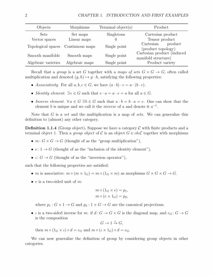
2 CHAPTER 1. INTRODUCTION AND FIRST EXAMPLES
Objects Morphisms Terminal object(s) Product
Sets Set maps Singletons Cartesian productVector spaces Linear maps 0 Tensor product
Topological spaces Continuous maps Single pointCartesian product(product topology)
Smooth manifolds Smooth maps Single pointCartesian product (inducedmanifold structure)
Algebraic varieties Algebraic maps Single point Product variety
Recall that a group is a set G together with a maps of sets G × G → G, often calledmultiplication and denoted (g, h) 7→ g · h, satisfying the following properties:
• Associativity. For all a, b, c ∈ G, we have (a · b) · c = a · (b · c).
• Identity element. ∃ e ∈ G such that e · a = a · e = a for all a ∈ G.
• Inverse element. ∀ a ∈ G ∃ b ∈ G such that a · b = b · a = e. One can show that theelement b is unique and we call it the inverse of a and denote it a−1.
Note that G is a set and the multiplication is a map of sets. We can generalize thisdefinition to (almost) any other category.
Definition 1.1.4 (Group object). Suppose we have a category C with finite products and aterminal object 1. Then a group object of C is an object G ∈ ob C together with morphisms
• m : G×G→ G (thought of as the “group multiplication”),
• e : 1→ G (thought of as the “inclusion of the identity element”),
• ι : G→ G (thought of as the “inversion operator”),
such that the following properties are satisfied:
• m is associative: m ◦ (m× 1G) = m ◦ (1G ×m) as morphisms G×G×G→ G.
• e is a two-sided unit of m:
m ◦ (1G × e) = p1,
m ◦ (e× 1G) = p2,
where p1 : G× 1→ G and p2 : 1×G→ G are the canonical projections.
• ι is a two-sided inverse for m: if d : G→ G×G is the diagonal map, and eG : G→ Gis the composition
G→ 1e−→ G,
then m ◦ (1G × ι) ◦ d = eG and m ◦ (ι× 1G) ◦ d = eG.
We can now generalize the definition of group by considering group objects in othercategories.
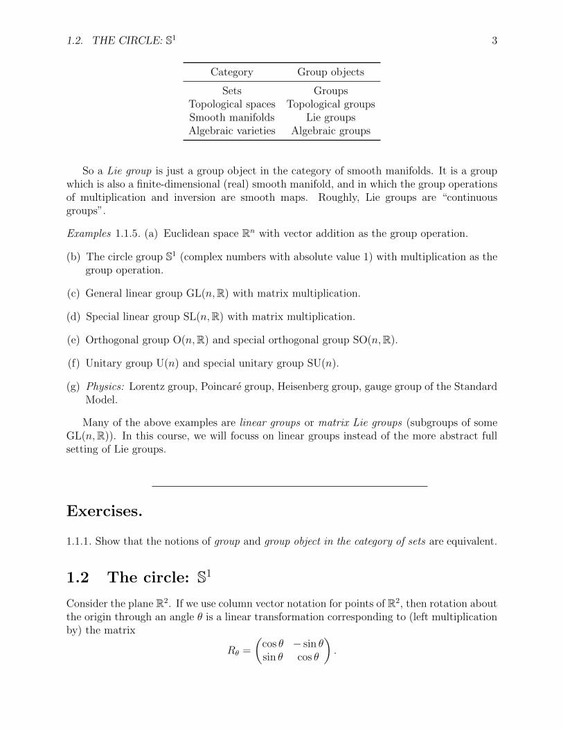
1.2. THE CIRCLE: S1 3
Category Group objects
Sets GroupsTopological spaces Topological groupsSmooth manifolds Lie groupsAlgebraic varieties Algebraic groups
So a Lie group is just a group object in the category of smooth manifolds. It is a groupwhich is also a finite-dimensional (real) smooth manifold, and in which the group operationsof multiplication and inversion are smooth maps. Roughly, Lie groups are “continuousgroups”.
Examples 1.1.5. (a) Euclidean space Rn with vector addition as the group operation.
(b) The circle group S1 (complex numbers with absolute value 1) with multiplication as thegroup operation.
(c) General linear group GL(n,R) with matrix multiplication.
(d) Special linear group SL(n,R) with matrix multiplication.
(e) Orthogonal group O(n,R) and special orthogonal group SO(n,R).
(f) Unitary group U(n) and special unitary group SU(n).
(g) Physics: Lorentz group, Poincare group, Heisenberg group, gauge group of the StandardModel.
Many of the above examples are linear groups or matrix Lie groups (subgroups of someGL(n,R)). In this course, we will focuss on linear groups instead of the more abstract fullsetting of Lie groups.
Exercises.
1.1.1. Show that the notions of group and group object in the category of sets are equivalent.
1.2 The circle: S1
Consider the plane R2. If we use column vector notation for points of R2, then rotation aboutthe origin through an angle θ is a linear transformation corresponding to (left multiplicationby) the matrix
Rθ =
(cos θ − sin θsin θ cos θ
).

4 CHAPTER 1. INTRODUCTION AND FIRST EXAMPLES
This rotation corresponds to the map(xy
)7→ Rθ
(xy
)=
(x cos θ − y sin θx sin θ + y cos θ
).
Rotating first by θ and then by ϕ corresponds to multiplication by Rθ and then by Rϕ or,equivalently, by RϕRθ. So composition of rotation corresponds to multiplication of matrices.
Definition 1.2.1 (SO(2)). The group {Rθ | θ ∈ R} is called the special orthogonal groupSO(2). The term special refers to the fact that their determinant is one (check!) and theterm orthogonal refers to the fact that they do not change distances (or that RθR
Tθ = 1 for
any θ) – we will come back to this issue later.
Another way of viewing the plane is as the set of complex numbers C. Then the point(x, y) corresponds to the complex number x+ iy. Then rotation by θ corresponds to multi-plication by
zθ = cos θ + i sin θ
since
zθ(x+ iy) = (cos θ + i sin θ)(x+ iy)
= x cos θ − y sin θ + i(x sin θ + y cos θ).
Composition of rotations corresponds to multiplication of complex numbers since rotatingby θ and then by ϕ is the same as multiplying by zϕzθ.
Note thatS1 := {zθ | θ ∈ R}
is the precisely the set of complex numbers of absolute value 1. Thus S1 is the circle of radius1 centred at the origin. Therefore, S1 has a geometric structure (as a circle) and a groupstructure (via multiplication of complex numbers). The multiplication and inverse maps areboth smooth and so S1 is a Lie group.
Definition 1.2.2 (Matrix group and linear group). A matrix group is a set of invertiblematrices that is closed under multiplication and inversion. A linear group is a group that isisomorphic to a matrix group.
Remark 1.2.3. Some references use the term linear group to mean a group consisting ofmatrices (i.e. a matrix group as defined above).
Example 1.2.4. We see that SO(2) is a matrix group. Since S1 is isomorphic (as a group) toSO(2) (Exercise 1.2.2), S1 is a linear group.
1.3. MATRIX REPRESENTATIONS OF COMPLEX NUMBERS 5
Exercises.
1.2.1. Verify that if u, v ∈ R2 and R ∈ SO(2), then the distance between the points u and vis the same as the distance between the points Ru and Rv.
1.2.2. Prove that the map zθ 7→ Rθ, θ ∈ R, is a group isomorphism from S1 to SO(2).
1.3 Matrix representations of complex numbers
Define
1 =
(1 00 1
), i =
(0 −11 0
).
The set of matrices
C := {a1 + bi | a, b ∈ R} =
{(a −bb a
) ∣∣∣∣ a, b ∈ R}
is closed under addition and multiplication, and hence forms a subring of M2(R) (Exer-cise 1.3.1).
Theorem 1.3.1. The map
C→ C, a+ bi 7→ a1 + bi,
is a ring isomorphism.
Proof. It is easy to see that it is a bijective map that commutes with addition and scalarmultiplication. Since we have
12 = 1, 1i = i1 = i, i2 = −1,
it is also a ring homomorphism.
Remark 1.3.2. Theorem 1.3.1 will allow us to convert from matrices with complex entries to(larger) matrices with real entries.
Note that the squared absolute value |a+ bi|2 = a2 + b2 is the determinant of the corre-
sponding matrix
(a −bb a
). Let z1, z2 be two complex numbers with corresponding matrices
A1, A2. Then
|z1|2|z2|2 = detA1 detA2 = det(A1A2) = |z1z2|2,
and thus
|z1||z2| = |z1z2|.
So multiplicativity of the absolute value corresponds to multiplicativity of determinants.
6 CHAPTER 1. INTRODUCTION AND FIRST EXAMPLES
Note also that if z ∈ C corresponds to the matrix A, then
z−1 =a− bia2 + b2
corresponds to the inverse matrix(a −bb a
)−1
=1
a2 + b2
(a b−b a
).
Of course, this also follows from the ring isomorphism above.
Exercises.
1.3.1. Show that the set of matrices
C := {a1 + bi | a, b ∈ R} =
{(a −bb a
) ∣∣∣∣ a, b ∈ R}
is closed under addition and multiplication and hence forms a subring of Mn(R).
1.4 Quaternions
Definition 1.4.1 (Quaternions). Define a multiplication on the real vector space with basis{1, i, j, k} by
1i = i1 = i, 1j = j1 = j, 1k = k1 = k,
ij = −ji = k, jk = −kj = i, ki = −ik = j,
12 = 1, i2 = j2 = k2 = −1,
and extending by linearity. The elements of the resulting ring (or algebra) H are calledquaternions .
Strictly speaking, we need to check that the multiplication is associative and distributiveover addition before we know it is a ring (but see below). Note that the quaternions are notcommutative.
We would like to give a matrix realization of quaternions like we did for the complexnumbers. Define 2× 2 complex matrices
1 =
(1 00 1
), i =
(0 −11 0
), j =
(0 −i−i 0
), k =
(i 00 −i
).
Then define
H = {a1 + bi + cj + dk | a, b, c, d ∈ R} =
{(a+ di −b− cib− ci a− di
) ∣∣∣∣ a, b, c, d ∈ R}
1.4. QUATERNIONS 7
=
{(z w−w z
) ∣∣∣∣ z, w ∈ C}.
The mapH→ H, a+ bi+ cj + dk 7→ a1 + bi + cj + dk, (1.1)
is an isomorphism of additive groups that commutes with the multiplication (Exercise 1.4.1).It follows that the quaternions satisfy the following properties.
Addition:
• Commutativity. q1 + q2 = q2 + q1 for all q1, q2 ∈ H.
• Associativity. q1 + (q2 + q3) = (q1 + q2) + q3 for all q1, q2, q3 ∈ H.
• Inverse law. q + (−q) = 0 for all q ∈ H.
• Identity law. q + 0 = q for all q ∈ H.
Multiplication:
• Associativity. q1(q2q3) = (q1q2)q3 for all q1, q2, q3 ∈ H.
• Inverse law. qq−1 = q−1q = 1 for q ∈ H, q 6= 0. Here q−1 is the quaternion correspond-ing to the inverse of the matrix corresponding to q.
• Identity law. 1q = q1 = q for all q ∈ H.
• Left distributive law. q1(q2 + q3) = q1q2 + q1q3 for all q1, q2, q3 ∈ H.
• Right distributive law. (q2 + q3)q1 = q2q1 + q3q1 for all q1, q2, q3 ∈ H.
In particular, H is a ring. We need the right and left distributive laws because H is notcommutative.
Remark 1.4.2. Note that C is a subring of H (spanned by 1 and i).
Following the example of complex numbers, we define the absolute value of the quaternionq = a+ bi+ cj+ dk to be the (positive) square root of the determinant of the correspondingmatrix. That is
|q|2 = det
(a+ id −b− icb− ic a− id
)= a2 + b2 + c2 + d2.
In other words, |q| is the distance of the point (a, b, c, d) from the origin in R4.As for complex numbers, multiplicativity of the determinant implies multiplicativity of
absolute values of quaternions:
|q1q2| = |q1||q2| for all q ∈ H.
From our identification with matrices, we get an explicit formula for the inverse. Ifq = a+ bi+ cj + dk, then
q−1 =1
a2 + b2 + c2 + d2(a− bi− cj − dk).
8 CHAPTER 1. INTRODUCTION AND FIRST EXAMPLES
If q = a+ bi+ cj + dk, then q := a− bi− cj − dk is called the quaternion conjugate of q.So we have
qq = qq = a2 + b2 + c2 + d2 = |q|2.
Because of the multiplicative property of the absolute value of quaternions, the 3-sphereof unit quaternions
{q ∈ H | |q| = 1} = {a+ bi+ cj + dk | a2 + b2 + c2 + d2 = 1}
is closed under multiplication. Since H can be identified with R4, this shows that S3 is agroup under quaternion multiplication (just like S1 is group under complex multiplication).
If X is a matrix with complex entries, we define X∗ to be the matrix obtained from thetranspose XT by taking the complex conjugate of all entries.
Definition 1.4.3 (U(n) and SU(n)). A matrix X ∈ Mn(C) is called unitary if X∗X = In.The unitary group U(n) is the subgroup of GL(n,C) consisting of unitary matrices. Thespecial unitary group SU(n) is the subgroup of U(n) consisting of matrices of determinant 1.
Remark 1.4.4. Note that X∗X = I implies that | detX| = 1.
Proposition 1.4.5. The group S3 of unit quaternions is isomorphic to SU(2).
Proof. Recall that under our identification of quaternions with matrices, absolute valuecorresponds to the determinant. Therefore, the group of unit quaternions is isomorphic tothe matrix group {
Q =
(z w−w z
) ∣∣∣∣ detQ = 1
}.
Now, if Q =
(z wx y
), w, x, y, z ∈ C, and detQ = 1, then Q−1 =
(y −w−x z
). Therefore
Q∗ = Q−1 ⇐⇒(z xw y
)=
(y −w−x z
)⇐⇒ y = z, w = −x
and the result follows.
Exercises.
1.4.1. Show that the map (1.1) is an isomorphism of additive groups that commutes withthe multiplication.
1.4.2. Show that if q ∈ H corresponds to the matrix A, then q corresponds to the matrix A∗.Show that it follows that
q1q2 = q2q1.
1.5. QUATERNIONS AND SPACE ROTATIONS 9
1.5 Quaternions and space rotations
The pure imaginary quaternions
Ri+ Rj + Rk := {bi+ cj + dk | b, c, d ∈ R}
form a three-dimensional subspace of H, which we will often simply denote by R3 when thecontext is clear. This subspace is not closed under multiplication. An easy computationshows that
(u1i+ u2j + u3k)(v1i+ v2j + v3k)
= −(u1v1 + u2v2 + u3v3) + (u2v3 − u3v2)i− (u1v3 − u3v1)j + (u1v2 − u2v1)k.
If we identify the space of pure imaginary quaternions with R3 by identifying i, j, k with thestandard unit vectors, we see that
uv = −u · v + u× v,
where u× v is the vector cross product.Recall that u× v = 0 if u and v are parallel (i.e. if one is a scalar multiple of the other).
Thus, if u is a pure imaginary quaterion, we have
u2 = −u · u = −|u|2.
So if u is a unit vector in Ri+Rj+Rk, then u2 = −1. So every unit vector in Ri+Rj+Rkis a square root of −1.
Lett = t0 + t1i+ t2j + t3k ∈ H, |t| = 1.
LettI = t1i+ t2j + t3k
be the imaginary part of t. We have
t = t0 + tI , 1 = |t|2 = t20 + t21 + t22 + t23 = t20 + |tI |2.
Therefore, (t0, |tI |) is a point on the unit circle and so there exists θ such that
t0 = cos θ, |tI | = sin θ
and
t = cos θ +tI|tI ||tI | = cos θ + u sin θ
where
u =tI|tI |
is a unit vector in Ri+ Rj + Rk and hence u2 = −1.We want to associate to the unit quaternion t a rotation of R3. However, this cannot
be simply by multiplication by t since this would not preserve R3. However, note that
10 CHAPTER 1. INTRODUCTION AND FIRST EXAMPLES
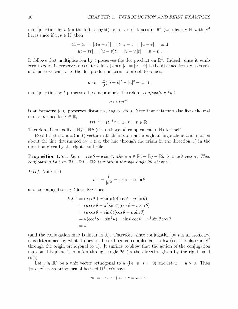
multiplication by t (on the left or right) preserves distances in R4 (we identify H with R4
here) since if u, v ∈ H, then
|tu− tv| = |t(u− v)| = |t||u− v| = |u− v|, and
|ut− vt| = |(u− v)t| = |u− v||t| = |u− v|.
It follows that multiplication by t preserves the dot product on R4. Indeed, since it sendszero to zero, it preserves absolute values (since |u| = |u− 0| is the distance from u to zero),and since we can write the dot product in terms of absolute values,
u · v =1
2(|u+ v|2 − |u|2 − |v|2),
multiplication by t preserves the dot product. Therefore, conjugation by t
q 7→ tqt−1
is an isometry (e.g. preserves distances, angles, etc.). Note that this map also fixes the realnumbers since for r ∈ R,
trt−1 = tt−1r = 1 · r = r ∈ R.Therefore, it maps Ri+ Rj + Rk (the orthogonal complement to R) to itself.
Recall that if u is a (unit) vector in R, then rotation through an angle about u is rotationabout the line determined by u (i.e. the line through the origin in the direction u) in thedirection given by the right hand rule.
Proposition 1.5.1. Let t = cos θ + u sin θ, where u ∈ Ri+ Rj + Rk is a unit vector. Thenconjugation by t on Ri+ Rj + Rk is rotation through angle 2θ about u.
Proof. Note that
t−1 =t
|t|2= cos θ − u sin θ
and so conjugation by t fixes Ru since
tut−1 = (cos θ + u sin θ)u(cos θ − u sin θ)
= (u cos θ + u2 sin θ)(cos θ − u sin θ)
= (u cos θ − sin θ)(cos θ − u sin θ)
= u(cos2 θ + sin2 θ)− sin θ cos θ − u2 sin θ cos θ
= u
(and the conjugation map is linear in R). Therefore, since conjugation by t is an isometry,it is determined by what it does to the orthogonal complement to Ru (i.e. the plane in R3
through the origin orthogonal to u). It suffices to show that the action of the conjugationmap on this plane is rotation through angle 2θ (in the direction given by the right handrule).
Let v ∈ R3 be a unit vector orthogonal to u (i.e. u · v = 0) and let w = u × v. Then{u, v, w} is an orthonormal basis of R3. We have
uv = −u · v + u× v = u× v.
1.5. QUATERNIONS AND SPACE ROTATIONS 11
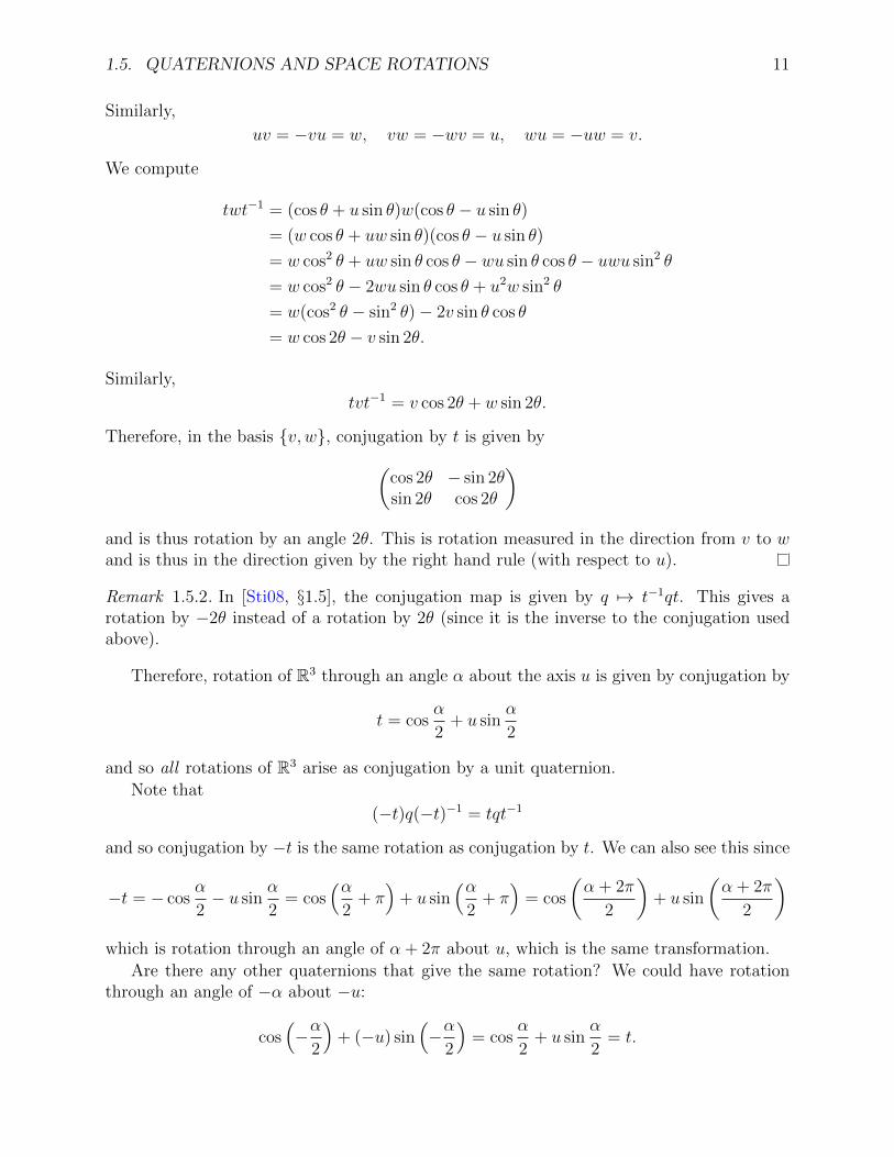
Similarly,
uv = −vu = w, vw = −wv = u, wu = −uw = v.
We compute
twt−1 = (cos θ + u sin θ)w(cos θ − u sin θ)
= (w cos θ + uw sin θ)(cos θ − u sin θ)
= w cos2 θ + uw sin θ cos θ − wu sin θ cos θ − uwu sin2 θ
= w cos2 θ − 2wu sin θ cos θ + u2w sin2 θ
= w(cos2 θ − sin2 θ)− 2v sin θ cos θ
= w cos 2θ − v sin 2θ.
Similarly,
tvt−1 = v cos 2θ + w sin 2θ.
Therefore, in the basis {v, w}, conjugation by t is given by(cos 2θ − sin 2θsin 2θ cos 2θ
)and is thus rotation by an angle 2θ. This is rotation measured in the direction from v to wand is thus in the direction given by the right hand rule (with respect to u).
Remark 1.5.2. In [Sti08, §1.5], the conjugation map is given by q 7→ t−1qt. This gives arotation by −2θ instead of a rotation by 2θ (since it is the inverse to the conjugation usedabove).
Therefore, rotation of R3 through an angle α about the axis u is given by conjugation by
t = cosα
2+ u sin
α
2
and so all rotations of R3 arise as conjugation by a unit quaternion.
Note that
(−t)q(−t)−1 = tqt−1
and so conjugation by −t is the same rotation as conjugation by t. We can also see this since
−t = − cosα
2− u sin
α
2= cos
(α2
+ π)
+ u sin(α
2+ π)
= cos
(α + 2π
2
)+ u sin
(α + 2π
2
)which is rotation through an angle of α + 2π about u, which is the same transformation.
Are there any other quaternions that give the same rotation? We could have rotationthrough an angle of −α about −u:
cos(−α
2
)+ (−u) sin
(−α
2
)= cos
α
2+ u sin
α
2= t.
12 CHAPTER 1. INTRODUCTION AND FIRST EXAMPLES
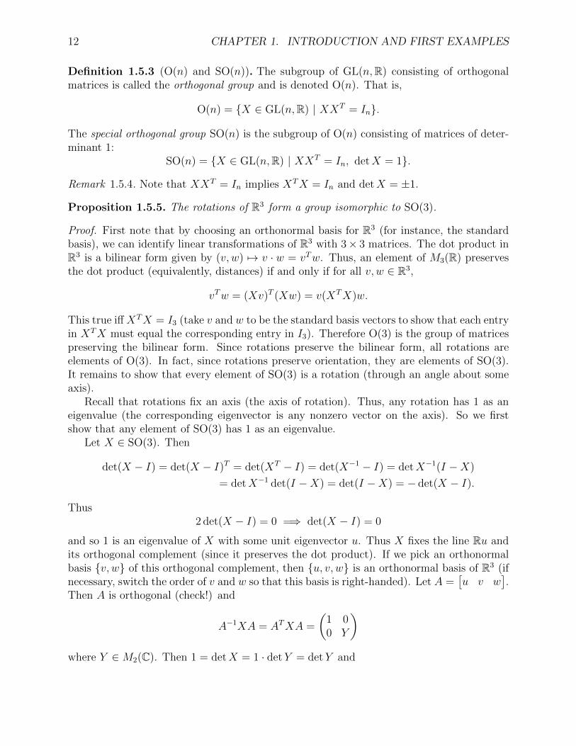
Definition 1.5.3 (O(n) and SO(n)). The subgroup of GL(n,R) consisting of orthogonalmatrices is called the orthogonal group and is denoted O(n). That is,
O(n) = {X ∈ GL(n,R) | XXT = In}.
The special orthogonal group SO(n) is the subgroup of O(n) consisting of matrices of deter-minant 1:
SO(n) = {X ∈ GL(n,R) | XXT = In, detX = 1}.
Remark 1.5.4. Note that XXT = In implies XTX = In and detX = ±1.
Proposition 1.5.5. The rotations of R3 form a group isomorphic to SO(3).
Proof. First note that by choosing an orthonormal basis for R3 (for instance, the standardbasis), we can identify linear transformations of R3 with 3× 3 matrices. The dot product inR3 is a bilinear form given by (v, w) 7→ v · w = vTw. Thus, an element of M3(R) preservesthe dot product (equivalently, distances) if and only if for all v, w ∈ R3,
vTw = (Xv)T (Xw) = v(XTX)w.
This true iff XTX = I3 (take v and w to be the standard basis vectors to show that each entryin XTX must equal the corresponding entry in I3). Therefore O(3) is the group of matricespreserving the bilinear form. Since rotations preserve the bilinear form, all rotations areelements of O(3). In fact, since rotations preserve orientation, they are elements of SO(3).It remains to show that every element of SO(3) is a rotation (through an angle about someaxis).
Recall that rotations fix an axis (the axis of rotation). Thus, any rotation has 1 as aneigenvalue (the corresponding eigenvector is any nonzero vector on the axis). So we firstshow that any element of SO(3) has 1 as an eigenvalue.
Let X ∈ SO(3). Then
det(X − I) = det(X − I)T = det(XT − I) = det(X−1 − I) = detX−1(I −X)
= detX−1 det(I −X) = det(I −X) = − det(X − I).
Thus2 det(X − I) = 0 =⇒ det(X − I) = 0
and so 1 is an eigenvalue of X with some unit eigenvector u. Thus X fixes the line Ru andits orthogonal complement (since it preserves the dot product). If we pick an orthonormalbasis {v, w} of this orthogonal complement, then {u, v, w} is an orthonormal basis of R3 (ifnecessary, switch the order of v and w so that this basis is right-handed). Let A =
[u v w
].
Then A is orthogonal (check!) and
A−1XA = ATXA =
(1 00 Y
)where Y ∈M2(C). Then 1 = detX = 1 · detY = detY and
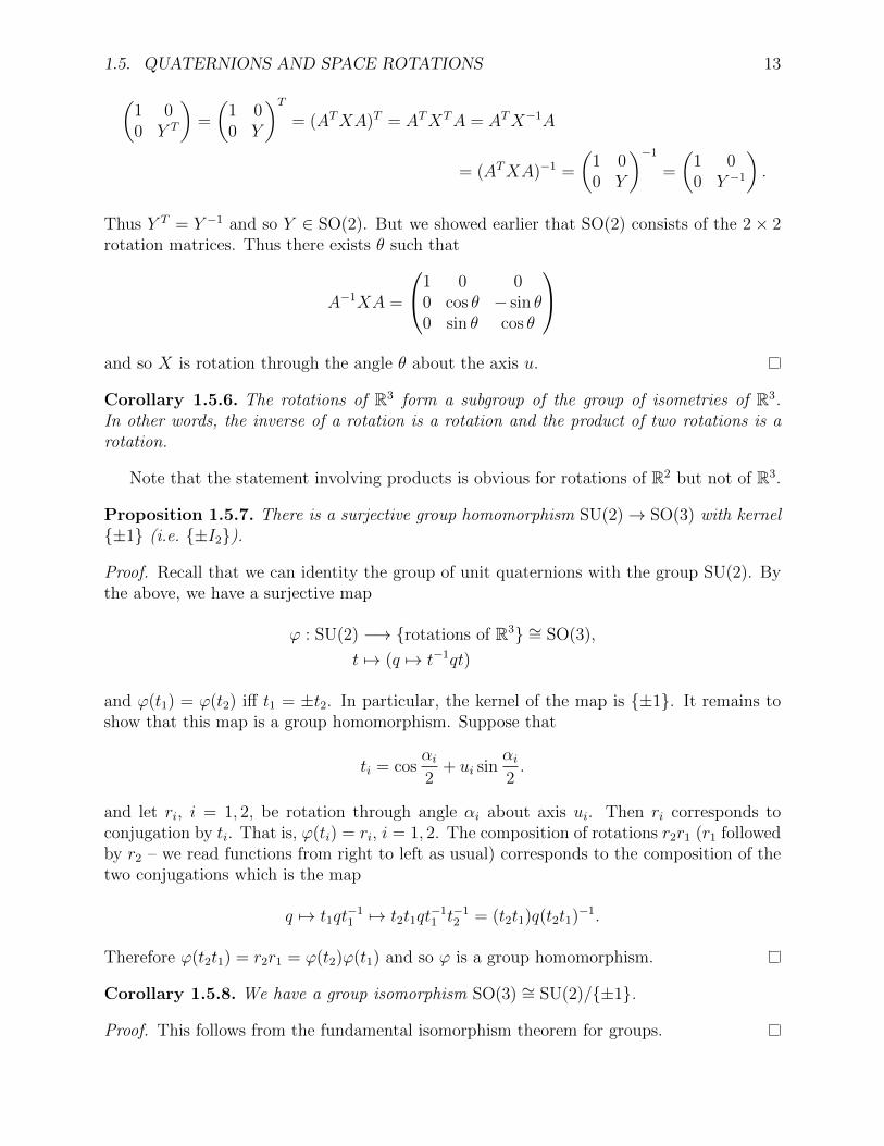
1.5. QUATERNIONS AND SPACE ROTATIONS 13
(1 00 Y T
)=
(1 00 Y
)T= (ATXA)T = ATXTA = ATX−1A
= (ATXA)−1 =
(1 00 Y
)−1
=
(1 00 Y −1
).
Thus Y T = Y −1 and so Y ∈ SO(2). But we showed earlier that SO(2) consists of the 2× 2rotation matrices. Thus there exists θ such that
A−1XA =
1 0 00 cos θ − sin θ0 sin θ cos θ
and so X is rotation through the angle θ about the axis u.
Corollary 1.5.6. The rotations of R3 form a subgroup of the group of isometries of R3.In other words, the inverse of a rotation is a rotation and the product of two rotations is arotation.
Note that the statement involving products is obvious for rotations of R2 but not of R3.
Proposition 1.5.7. There is a surjective group homomorphism SU(2)→ SO(3) with kernel{±1} (i.e. {±I2}).
Proof. Recall that we can identity the group of unit quaternions with the group SU(2). Bythe above, we have a surjective map
ϕ : SU(2) −→ {rotations of R3} ∼= SO(3),
t 7→ (q 7→ t−1qt)
and ϕ(t1) = ϕ(t2) iff t1 = ±t2. In particular, the kernel of the map is {±1}. It remains toshow that this map is a group homomorphism. Suppose that
ti = cosαi2
+ ui sinαi2.
and let ri, i = 1, 2, be rotation through angle αi about axis ui. Then ri corresponds toconjugation by ti. That is, ϕ(ti) = ri, i = 1, 2. The composition of rotations r2r1 (r1 followedby r2 – we read functions from right to left as usual) corresponds to the composition of thetwo conjugations which is the map
q 7→ t1qt−11 7→ t2t1qt
−11 t−1
2 = (t2t1)q(t2t1)−1.
Therefore ϕ(t2t1) = r2r1 = ϕ(t2)ϕ(t1) and so ϕ is a group homomorphism.
Corollary 1.5.8. We have a group isomorphism SO(3) ∼= SU(2)/{±1}.
Proof. This follows from the fundamental isomorphism theorem for groups.
14 CHAPTER 1. INTRODUCTION AND FIRST EXAMPLES
Remark 1.5.9. Recall that the elements of SU(2)/{±1} are cosets {±t} and multiplication isgiven by {±t1}{±t2} = {±t1t2}. The above corollary is often stated as “SU(2) is a doublecover of SO(3).” It has some deep applications to physics. If you “rotate” an electronthrough an angle of 2π it is not the same as what you started with. This is related tothe fact that electrons are described by representations of SU(2) and not SO(3). One canillustrate this idea with Dirac’s belt trick .
Proposition 1.5.7 allows one to identify rotations of R3 with pairs ±t of antipodal unitquaternions. One can thus do things like compute the composition of rotations (and findthe axis and angle of the composition) via quaternion arithmetic. This is actually done inthe field of computer graphics.
Recall that a subgroup H of a group G is called normal if gHg−1 = H for all g ∈ G.Normal subgroups are precisely those subgroups that arise as kernels of homomorphisms. Agroup G is simple if its only normal subgroups are the trivial subgroup and G itself.
Proposition 1.5.10 (Simplicity of SO(3)). The group SO(3) is simple.
Proof. See [Sti08, p. 33]. We will return to this issue later with a different proof (seeCorollary 5.14.7).
1.6 Isometries of Rn and reflections
We now want to give a description of rotations in R4 via quaternions. We first prove someresults about isometries of Rn in general. Recall that an isometry of Rn is a map f : Rn → Rn
such that
|f(u)− f(v)| = |u− v|, ∀ u, v ∈ Rn.
Thus, isometries are maps that preserve distance. As we saw earlier, preserving dot productsis the same as preserving distance and fixing the origin.
Definition 1.6.1. A hyperplane H through O is an (n − 1)-dimensional subspace of Rn,and reflection in H is the linear endomorphism of Rn that fixes the points of H and reversesvectors orthogonal to H.
We can give an explicit formula for reflection ru in the hyperplane orthogonal to a(nonzero) vector u. It is
ru(v) = v − 2v · u|u|2
u, v ∈ Rn. (1.2)
Theorem 1.6.2 (Cartan–Dieudonne Theorem). Any isometry of Rn that fixes the origin Ois the product of at most n reflections in hyperplanes through O.
Note: There is an error in the proof of this result given in [Sti08, p. 36]. It states there thatruf is the identity on Ru when it should be Rv.
Proof. We prove the result by induction on n.
1.6. ISOMETRIES OF RN AND REFLECTIONS 15
Base case (n = 1). The only isometries of R fixing O are the identity and the mapx 7→ −x, which is reflection in O (a hyperplane in R).
Inductive step. Suppose the result is true for n = k − 1 and let f be an isometry of Rk
fixing O. If f is the identity, we’re done. Therefore, assume f is not the identity. Then thereexists v ∈ Rk such that f(v) = w 6= v. Let ru be the reflection in the hyperplane orthogonalto u = v − w. Then
ru(w) = w − 2w · u|u|2
u = w − 2w · (v − w)
|v − w|2(v − w)
= w − 2w · v − w · w
v · v − 2w · v + w · w(v − w)
= w − 2w · v − w · w
2w · w − 2w · v(v − w) (since v · v = f(v) · f(v) = w · w)
= w + (v − w) = v.
Thus ruf(v) = ru(w) = v and so v is fixed by ruf . Since isometries are linear transformations,ruf is the identity on the subspace Rv of Rn and is determined by its restriction g to theRk−1 orthogonal to Rv. By induction, g is the product of ≤ k − 1 reflections. Thereforef = rug is the product of ≤ k reflections.
Remark 1.6.3. The full Cartan–Dieudonne Theorem is actually more general, concerningisometries of n-dimensional vector spaces over a field of characteristic not equal to 2 with anon-degenerate bilinear form. What we proved above is just a special case.
Definition 1.6.4 (Orientation-preserving and orientation-reversing). A linear map is calledorientation-preserving if its determinant is positive and orientation-reversing otherwise.
Reflections are linear and have determinant −1. To see this, pick a basis compatible withthe reflection, i.e. a basis {v1, . . . , vn} where {v1, . . . , vn−1} span the hyperplane of reflectionand vn is orthogonal to the hyperplane of reflection. Then in this basis, the reflection isdiagonal with diagonal entries 1, . . . , 1,−1.
So we see that a product of reflections is orientation-preserving iff it contains an evennumber of terms.
Definition 1.6.5 (Rotation). A rotation of Rn about O is an orientation-preserving isometrythat fixes O.
It follows that if we choose an orthonormal basis of Rn (for instance, the standard basis)so that linear maps correspond to n× n matrices, the rotations of Rn correspond to SO(n).
Exercises.
16 CHAPTER 1. INTRODUCTION AND FIRST EXAMPLES
1.6.1. Verify that the map ru defined by (1.2) is indeed reflection in the hyperlane orthogonalto the nonzero vector U . (It helps to draw a picture.) Note that it suffices to show that theright hand side maps u to u and fixes any vector orthogonal to u.
1.7 Quaternions and rotations of R4
It follows from the Cartan–Dieudonne Theorem that any rotation of R4 is the product of 0,2, or 4 reflections. Recall that we identify the group of unit quaternions with SU(2) and Hwith R4.
Proposition 1.7.1. Let u ∈ SU(2) be a unit quaternion. The map
ru : H→ H, ru(q) = −uqu
is reflection in the hyperplane through O orthogonal to u.
Proof. Note that q 7→ −q is the map
a+ bi+ cj + dk 7→ −a+ bi+ cj + dk, a, b, c, d ∈ R
and is therefore reflection in the hyperplane Ri + Rj + Rk, which is an isometry. We sawbefore that left or right multiplication by a unit quaternion is an isometry and thus thecomposition
q 7→ −q 7→ −uq 7→ −uquis also an isometry. Now, for v ∈ H, we have
ru(vu) = −u(vu)u = −uuvu = −|u|2vu = −vu.
Therefore, we have
ru(u) = −u, ru(iu) = iu, ru(ju) = ju, ru(ku) = ku.
So ru reverses vectors parallel to u and fixes points in the space spanned by iu, ju and ku.Therefore, it suffices to show that iu, ju and ku span the hyperplane through O orthogonalto u. First note that if u = a+ bi+ cj + dk, then
u · iu = (a, b, c, d) · (−b, a,−d, c) = 0.
Similarly, one can show that u is also orthogonal to ju and ku. So it remains to show thatiu, ju and ku span a 3-dimensional subspace of H or, equivalently, that u, iu, ju, ku span allof H. But this is true since for any v ∈ H, we have
v = (vu−1)u
and we can express vu−1 as an R-linear combination of 1, i, j and k.
Proposition 1.7.2. The rotations of H = R4 about O are precisely the maps of the formq 7→ vqw, where v, w ∈ SU(2) are unit quaternions.
1.8. SU(2)× SU(2) AND SO(4) 17
Proof. We know that any rotation of H is a product of an even number of reflections. Thecomposition of reflections in the hyperplanes orthogonal to u1, u2, . . . , u2n ∈ SU(2) is themap
q 7→ −u1qu1 7→ −u2(−u1qu1)u2 = u2u1qu1u2 7→ . . . 7→ u2n · · · u3u2u1qu1u2u3 · · ·u2n.
Thus we have that this composition is the map q 7→ vqw where
v = u2n · · · u3u2u1, w = u1u2u3 · · ·u2n.
It follows that all rotations are of this form.It remains to show that all maps of the form q 7→ vqw for v, w ∈ SU(2) are rotations of
H about O. Since this map is the composition of left multiplication by v followed by rightmultiplication by w, it is enough to show that multiplication of H on either side by a unitquaternion is an orientation-preserving isometry (i.e. a rotation). We have already shownthat such a multiplication is an isometry, so we only need to show it is orientation-preserving.Let
v = a+ bi+ cj + dk, a2 + b2 + c2 + d2 = 1,
be an arbitrary unit quaternion. Then in the basis {1, i, j, k} of H = R4, left multiplicationby v has matrix
a −b −c −db a −d cc d a −bd −c b a
and one can verify by direct computation that this matrix has determinant one. The proofthat right multiplication by w is orientation-preserving is analogous.
1.8 SU(2)× SU(2) and SO(4)
Recall that the direct product G×H of groups G and H is the set
G×H = {(g, h) | g ∈ G, h ∈ H}
with multiplication(g1, h1) · (g2, h2) = (g1g2, h1h2).
The unit of G × H is (1G, 1H) where 1G is the unit of G and 1H is the unit of H and theinverse of (g, h) is (g−1, h−1).
If G is a group of n× n matrices and H is a group of m×m matrices, then the map
(g, h) 7→(g 00 h
)is an isomorphism from G×H to the group{(
g 00 h
) ∣∣∣∣ g ∈ G, h ∈ H}
18 CHAPTER 1. INTRODUCTION AND FIRST EXAMPLES
of block diagonal matrices (n+m)× (n+m) matrices since(g1 00 h1
)(g2 00 h2
)=
(g1g2 00 h1h2
).
For each pair of unit quaternions (v, w) ∈ SU(2)× SU(2), we know that the map
q 7→ vqw−1
is a rotation of H = R4 (since w−1 is also a unit quaterion) and is hence an element of SO(4).
Proposition 1.8.1. The map
ϕ : SU(2)× SU(2)→ SO(4), (v, w) 7→ (q 7→ vqw−1),
is a surjective group homomorphism with kernel {(1, 1), (−1,−1)}.
Proof. For q ∈ H,
ϕ((v1, w1)(v2, w2))(q) = ϕ(v1v2, w1w2)(q) = (v1v2)q(w1w2)−1
= v1(v2qw−12 )w−1
1 = ϕ(v1, w1)ϕ(v2, w2)(q).
Thereforeϕ((v1, w1)(v2, w2)) = ϕ(v1, w1)ϕ(v2, w2),
and so ϕ is a group homomorphism. It is surjective since we showed earlier that any rotationof R4 is of the form q 7→ vqw−1 for v, w ∈ SU(2).
Now suppose that (v, w) ∈ kerϕ. Then q 7→ vqw−1 is the identity map. In particular
v1w−1 = 1
and thus v = w. Therefore ϕ(v, w) = ϕ(v, v) is the map q 7→ vqv−1. We saw in ourdescription of rotations of R3 using quaternions that this map fixes the real axis and rotatesthe space of pure imaginary quaternions. We also saw that it is the identity map if and onlyif v = ±1.
Remark 1.8.2. Our convention here is slightly different from the one used in [Sti08]. Thatreference uses the map q 7→ v−1qw. This difference is analogous to one noted in the de-scription of rotations of R3 by quaternions (see Remark 1.5.2). Essentially, in [Sti08], thecomposition of rotations r1 and r2 is thought of as being r1r2 instead of r2r1. We use thelatter composition since it corresponds to the order in which you apply functions (right toleft).
Corollary 1.8.3. We have a group isomorphism (SU(2) × SU(2))/{±1} ∼= SO(4). Here1 = (1, 1) is the identity element of the product group SU(2)× SU(2) and −1 = (−1,−1).
Proof. This follows from the fundamental isomorphism theorem for groups.
Lemma 1.8.4. The group SO(4) is not simple.
1.8. SU(2)× SU(2) AND SO(4) 19
Proof. The subgroup SU(2) × {1} = {(v, 1) | v ∈ SU(2)} is the kernel of the group homo-morphism (v, w) 7→ (1, w), projection onto the second factor, and is thus a normal subgroupof SU(2)×SU(2). It follows that its image (under the map ϕ above) is a normal subgroup ofSO(4). This subgroup consists of the maps q 7→ vq. This subgroup is nontrivial and is notthe whole of SO(4) because since it does not contain the map q 7→ qw−1 for w 6= 1 (recallthat maps q 7→ v1qw
−11 and q 7→ v2qw
−12 are equal if and only if (v1, w1) = (±v1,±w1) by the
above corollary).
Chapter 2
Matrix Lie groups
In this chapter, we will study what is probably the most important class of Lie groups,matrix Lie groups. In addition to containing the important subclass of classical Lie groups ,focussing on matrix Lie groups (as opposed to abstract Lie groups) allows us to avoid muchdiscussion of abstract manifold theory.
2.1 Definitions
Recall that we can identify Mn(R) with Rn2and Mn(C) with Cn2
by interpreting the n2
entries
a11, a12, . . . , a1n, a21, . . . , a2n, . . . , an1, . . . , ann
as the coordinates of a point/matrix.
Definition 2.1.1 (Convergence of matrices). Let (Am)m∈N be a sequence of elements ofMn(C). We say that Am converges to a matrix A if each entry of Am converges (as m→∞)to the corresponding entry of A. That is, Am converges to A if
limm→∞
|(Am)k` − Ak`| = 0, ∀ 1 ≤ k, ` ≤ n.
Note that convergence in the above sense is the same as convergence in Cn2.
Definition 2.1.2 (Matrix Lie group). A matrix group is any subgroup of GL(n,C). Amatrix Lie group is any subgroup G of GL(n,C) with the following property: If (Am)m∈N isa sequence of matrices in G, and Am converges to some matrix A then either A ∈ G, or Ais not invertible.
Remark 2.1.3. The convergence condition on G in Definition 2.1.2 is equivalent to the condi-tion that G be a closed subset of GL(n,C). Note that this does not imply that G is a closedsubset of Mn(C). So matrix Lie groups are closed subgroups of GL(n,C).
Definition 2.1.4 (Linear group). A linear group is any group that is isomorphic to a matrixgroup. A linear Lie group is any group that is isomorphic to a matrix Lie group. We willsometimes abuse terminology and refer to linear Lie groups as matrix Lie groups.
20
2.2. FINITE GROUPS 21
Before discussing examples of matrix Lie groups, let us give a non-example. Let G bethe set of all n× n invertible matrices with (real) rational entries. Then, for example,
limm→∞
∑mk=0
1k!
0 · · · · · · 0
0 1. . .
......
. . . . . . . . ....
.... . . 1 0
0 · · · · · · 0 1
=
e 0 · · · · · · 0
0 1. . .
......
. . . . . . . . ....
.... . . 1 0
0 · · · · · · 0 1
,
which is invertible but not in G. Therefore G is not a matrix Lie group.We now discuss important examples of matrix Lie groups.
2.2 Finite groups
Suppose G is a finite subgroup of GL(n,C). Then any convergent sequence (Am)m∈N in G iseventually stable (i.e. there is some A ∈ G such that Am = A for m sufficiently large). ThusG is a matrix Lie group.
Recall that Sn is isomorphic to a subgroup of GL(n,C) as follows. Consider the standardbasis X = {e1, . . . , en} of Cn. Then permutations of this set correspond to elements ofGL(n,C). Thus Sn is a linear Lie group.
Any finite group G acts on itself (regarded as a set) by left multiplication. This yieldsan injective group homomorphism G→ SG and so G is isomorphic to a subgroup of SG and,hence, all finite groups are linear Lie groups.
2.3 The general and special linear groups
The complex general linear group GL(n,C) is certainly a subgroup of itself. If (Am)m∈Nis a sequence of matrices in GL(n,C) converging to A, then A is in GL(n,C) or A is notinvertible (by the definition of GL(n,C)). Therefore GL(n,C) is a matrix Lie group.
GL(n,R) is a subgroup of GL(n,C) and if Am is a sequence of matrices in GL(n,R)converging to A, then the entries of A are real. Thus either A ∈ GL(n,R) or A is notinvertible. Therefore the real general linear group GL(n,R) is a matrix Lie group.
The real special linear group SL(n,R) and complex special linear group SL(n,C) are bothsubgroups of GL(n,C). Suppose (Am)m∈N is a sequence of matrices in SL(n,R) or SL(n,C)converging to A. Since the determinant is a continuous function of the entries of a matrix,detA = 1. Therefore SL(n,R) and SL(n,C) are both matrix Lie groups.
2.4 The orthogonal and special orthogonal groups
Recall that we have an inner product (dot product) on Rn defined as follows. If u =(u1, . . . , un) and v = (v1, . . . , vn), then
u · v = uTv = u1v1 + · · ·+ unvn.
22 CHAPTER 2. MATRIX LIE GROUPS
(In the above, we view u and v as column vectors.) We have that |u|2 = u · u and we knowthat a linear transformation preserves length (or distance) if and only if it preserves the innerproduct. We showed that an n× n matrix X preserves the dot product if and only if
X ∈ O(n) = {A ∈ GL(n,R) | ATA = In}.
Since we defined rotations to be orientation preserving isometries, we have that X is arotation if and only if
X ∈ SO(n) = {A ∈ O(n) | detA = 1}.
One easily checks (Exercise 2.4.1) that the orthogonal group O(n) and special orthogonalgroup SO(n) are closely under multiplication and inversion and contain the identity matrix.For instance, if A,B ∈ O(n), then
(AB)T (AB) = BTATAB = BT IB = BTB = I.
Thus SO(n) is a subgroup of O(n) and both are subgroups of GL(n,C).Suppose (Am)m∈N is a sequence of matrices in O(n) converging to A. Since multiplication
of matrices is a continuous function (Exercise 2.4.2), we have that ATA = In and henceA ∈ O(n). Therefore O(n) is a matrix Lie group. Since the determinant is a continuousfunction, we see that SO(n) is also a matrix Lie group.
Remark 2.4.1. Note that we do not write O(n,R) because, by convention, O(n) alwaysconsists of real matrices.
Exercises.
2.4.1. Verify that SO(n) and O(n) are both subgroups of GL(n,C).
2.4.2. Show that multiplication of matrices is a continuous function in the entries of thematrices.
2.5 The unitary and special unitary groups
The unitary group
U(n) = {A ∈ GL(n,C) | AA∗ = In}, where (A∗)jk = Akj
is a subgroup of GL(n,C). The same argument used for the orthogonal and special orthogonalgroups shows that U(n) is a matrix Lie group, and so is the special unitary group
SU(n) = {A ∈ U(n) | detA = 1}.
2.6. THE COMPLEX ORTHOGONAL GROUPS 23
Remark 2.5.1. A unitary matrix can have determinant eiθ for any θ, whereas an orthogonalmatrix can only have determinant ±1. Thus SU(n) is a “smaller” subset of U(n) than SO(n)is of O(n).
Remark 2.5.2. For a real or complex matrix A, the condition AA∗ = I (which reduces toAAT = I if A is real) is equivalent to the condition A∗A = I. This follows from the standardresult in linear algebra that if A and B are square and AB = I, then B = A−1 (one doesn’tneed to check that BA = I as well).
Exercises.
2.5.1. For an arbitrary θ ∈ R, write down an element of U(n) with determinant eiθ.
2.5.2. Show that the unitary group is precisely the group of matrices preserving the bilinearform on Cn given by
〈x, y〉 = x1yn + · · ·+ xnyn.
2.6 The complex orthogonal groups
The complex orthogonal group is the subgroup
O(n,C) = {A ∈ GL(n,C) | AAT = In}
of GL(n,C). As above, we see that O(n,C) is a matrix Lie group and so is the specialcomplex orthogonal group
SO(n,C) = {A ∈ O(n,C) | detA = 1}.
Note that O(n,C) is the subgroup of GL(n,C) preserving the bilinear form on Cn givenby
〈x, y〉 = x1y1 + · · ·+ xnyn.
Note that this is not an inner product since it is symmetric rather than conjugate-symmetric.
2.7 The symplectic groups
We have a natural inner product on Hn given by
〈(p1, . . . , pn), (q1, . . . , qn)〉 = p1q1 + . . . pnqn.
Note that Hn is not a vector space over H since quaternions do not act properly as “scalars”since their multiplication is not commutative (H is not a field).
24 CHAPTER 2. MATRIX LIE GROUPS
Since quaternion multiplication is associative, matrix multiplication of matrices withquaternionic entries is associative. Therefore we can use them to define linear transformationsof Hn. We define the (compact) symplectic group Sp(n) to be the subset of Mn(H) consistingof those matrices that preserve the above bilinear form. That is,
Sp(n) = {A ∈Mn(H) | 〈Ap,Aq〉 = 〈p, q〉 ∀ p, q ∈ Hn}.
The proof of the following lemma is an exercise (Exercise 2.7.1). It follows from this lemmathat Sp(n) is a matrix Lie group.
Lemma 2.7.1. We have
Sp(n) = {A ∈Mn(H) | AA? = In}
where A? denotes the quaternion conjugate transpose of A.
Remark 2.7.2. Note that, for a quaternionic matrix A, the condition AA? = I is equivalentto the condition A?A = I. This follows from the fact that Sp(n) is a group, or from therealization of quaternionic matrices as complex matrices (see Section 1.4 and Remark 2.5.2).
Because H is not a field, it is often useful to express Sp(n) in terms of complex matrices.Recall that we can identify quaternions with matrices of the form(
α −ββ α
), α, β ∈ C.
Replacing the quaternion entries in A ∈ Mn(H) with the corresponding 2 × 2 complexmatrices produces a matrix in A ∈M2n(C) and this identification is a ring isomorphism.
Preserving the inner product means preserving length in the corresponding real spaceR4n. For example, Sp(1) consists of the 1× 1 quaternion matrices, multiplication by whichpreserves length in H = R4. We saw before that these are simply the unit quaternions, whichwe identified with SU(2). Therefore,
Sp(1) =
{(a+ id −b− icb− ic a− id
)∣∣∣∣ a2 + b2 + c2 + d2 = 1
}= SU(2).
We would like to know, for general values of n, which matrices in M2n(C) correspond toelements of Sp(n).
Define a skew-symmetric bilinear form B on R2n or C2n by
B((x1, y1, . . . , xn, yn), (x′1, y′1, . . . , x
′n, y
′n)) =
n∑k=1
xky′k − ykx′k.
Then the real symplectic group Sp(n,R) (respectively, complex symplectic group Sp(n,C)) isthe subgroup of GL(2n,R) (respectively, GL(2n,C)) consisting of matrices preserving B.
Let
J =
(0 1−1 0
),
2.8. THE HEISENBERG GROUP 25
and let
J2n =
J 0. . .
0 J
.
ThenB(x, y) = xTJ2ny
and
Sp(n,R) = {A ∈ GL(2n,R) | ATJ2nA = J2n},Sp(n,C) = {A ∈ GL(2n,C) | ATJ2nA = J2n}.
Note that we use the transpose (not the conjugate transpose) in the definition of Sp(n,C).For a symplectic (real or complex) matrix, we have
det J2n = det(ATJ2nA) = (detA)2 det J2n =⇒ detA = ±1.
In fact one can show that detA = 1 for A ∈ Sp(n,R) or A ∈ Sp(n,C). We will come backto this point later.
The proof of the following proposition is an exercise (see [Sti08, Exercises 3.4.1–3.4.3]).
Proposition 2.7.3. We have
Sp(n) = Sp(n,C) ∩ U(2n).
Remark 2.7.4. Some references write Sp(2n,C) for what we have denoted Sp(n,C).
Example 2.7.5 (The metaplectic group). There do exist Lie groups that are not matrix Liegroups. One example is the metaplectic group Mp(n,R), which is the unique connecteddouble cover (see Section 6.6) of the symplectic Lie group Sp(n,R). It is not a matrix Liegroup because it has no faithful finite-dimensional representations.
Exercises.
2.7.1. Prove Lemma 2.7.1.
2.8 The Heisenberg group
The Heisenberg group H is the set of all 3× 3 real matrices of the form
A =
1 a b0 1 c0 0 1
, a, b, c ∈ R.
26 CHAPTER 2. MATRIX LIE GROUPS
It is easy to check that I ∈ H and that H is closed under multiplication. Also
A−1 =
1 −a ac− b0 1 −c0 0 1
and so H is closed under inversion. It is clear that the limit of matrices in H is again in Hand so H is a matrix Lie group.
The name “Heisenberg group” comes from the fact that the Lie algebra of H satisfies theHeisenberg commutation relations of quantum mechanics.
2.9 The groups R∗, C∗, S1 and Rn
The groups R∗ and C∗ under matrix multiplication are isomorphic to GL(1,R) and GL(1,C),respectively, and so we view them as matrix Lie groups. The group S1 of complex numberswith absolute value one is isomorphic to U(1) and so we also view it as a matrix Lie group.
The group Rn under vector addition is isomorphic to the group of diagonal real matriceswith positive diagonal entries, via the map
(x1, . . . , xn) 7→
ex1 0
. . .
0 exn
.
One easily checks that this is a matrix Lie group and thus we view Rn as a matrix Lie groupas well.
2.10 The Euclidean group
The Euclidean group E(n) is the group of all one-to-one, onto, distance-preserving mapsfrom Rn to itself:
E(n) = {f : Rn → Rn | |f(x)− f(y)| = |x− y| ∀ x, y ∈ Rn}.
Note that we do not require these maps to be linear.The orthogonal group O(n) is the subgroup of E(n) consisting of all linear distance-
preserving maps of Rn to itself. For x ∈ Rn, define translation by x, denoted Tx, by
Tx(y) = x+ y.
The set of all translations is a subgroup of E(n).
Proposition 2.10.1. Every element of E(n) can be written uniquely in the form
TxR, x ∈ Rn, R ∈ O(n).
Proof. The proof of this proposition can be found in books on Euclidean geometry.
2.11. HOMOMORPHISMS OF LIE GROUPS 27
One can show (Exercise 2.10.2) that the Euclidean group is isomorphic to a matrix Liegroup.
Exercises.
2.10.1. Show that, for x1, x2 ∈ Rn and R1, R2 ∈ O(n), we have
(Tx1R1)(Tx2R2) = Tx1+R1x2(R1R2)
and that, for x ∈ Rn and R ∈ O(n), we have
(TxR)−1 = T−R−1xR−1.
This shows that E(n) is a semidirect product of the group of translations and the group O(n).More precisely, E(n) is isomorphic to the group consisting of pairs (Tx, R), for x ∈ Rn andR ∈ O(n), with multiplication
(x1, R1)(x2, R2) = (x1 +R1x2, R1R2).
2.10.2. Show that the map E(n)→ GL(n+ 1,R) given by
TxR 7→
x1
R...xn
0 · · · 0 1
is a one-to-one group homomorphism and conclude that E(n) is isomorphic to a matrix Liegroup.
2.11 Homomorphisms of Lie groups
Whenever one introduces a new type of mathematical object, one should define the allowedmaps between objects (more precisely, one should define a category).
Definition 2.11.1 (Lie group homomorphism/isomorphism). Let G and H be (matrix) Liegroups. A map Φ from G to H is called a Lie group homomorphism if
(a) Φ is a group homomorphism, and
(b) Φ is continuous.
If, in addition, Φ is one-to-one and onto and the inverse map Φ−1 is continuous, then Φ is aLie group isomorphism.
Examples 2.11.2. (a) The map R→ U(1) given by θ 7→ eiθ is a Lie group homomorphism.
28 CHAPTER 2. MATRIX LIE GROUPS
(b) The map U(1)→ SO(2) given by
eiθ 7→(
cos θ − sin θsin θ cos θ
)is a Lie group isomorphism (you should check that this map is well-defined and is indeedan isomorphism).
(c) Composing the previous two examples gives the Lie algebra homomorphism R→ SO(2)defined by
θ 7→(
cos θ − sin θsin θ cos θ
).
(d) The determinant is a Lie group homomorphism GL(n,C)→ C∗.
(e) The map SU(2) → SO(3) of Proposition 1.5.7 is continuous and is thus a Lie grouphomomorphism (recall that this map has kernel {±1}).
Chapter 3
Topology of Lie groups
In this chapter, we discuss some topological properties of Lie groups, including connectednessand compactness.
3.1 Connectedness
An important notion in theory of Lie groups is that of path-connectedness.
Definition 3.1.1 (Path-connected). Let A be a subset of Rn. A path in A is a continuousmap γ : [0, 1] → A. We say A is path-connected if, for any two points a, b ∈ A, there is apath γ in A such that γ(0) = a and γ(1) = b.
Remark 3.1.2. If γ : [a, b] → A, a < b, is a continuous map, we can always rescale to obtaina path γ : [0, 1]→ A. Therefore, we will sometimes also refer to these more general maps aspaths.
Remark 3.1.3. For those who know some topology, you know that the notion of path-connectedness is not the same, in general, as the notion of connectedness. However, it turnsout that a matrix Lie group is connected if and only if it is path-connected. (This followsfrom the fact that matrix Lie groups are manifolds, and hence are locally path-connected.)Thus we will sometimes ignore the difference between the two concepts in this course.
The property of being connected by some path is an equivalence relation on the set ofpoints of a matrix Lie group. The equivalence classes are the (connected) components of thematrix Lie group. Thus, the components have the property that two elements of the samecomponent can be joined by a continuous path but two elements of different componentscannot.
The proof of the following proposition is an exercise (see [Sti08, Exercises 3.2.1–3.2.3]).
Proposition 3.1.4. If G is a matrix Lie group, then the component of G containing theidentity is a subgroup of G.
Proposition 3.1.5. The group GL(n,C) is connected for all n ≥ 1.
29
30 CHAPTER 3. TOPOLOGY OF LIE GROUPS
We will give two proofs, one explicit and one not explicit (but shorter).
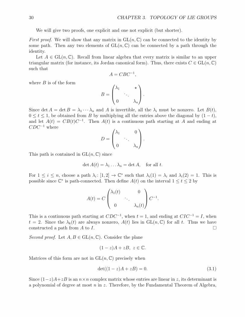
First proof. We will show that any matrix in GL(n,C) can be connected to the identity bysome path. Then any two elements of GL(n,C) can be connected by a path through theidentity.
Let A ∈ GL(n,C). Recall from linear algebra that every matrix is similar to an uppertriangular matrix (for instance, its Jordan canonical form). Thus, there exists C ∈ GL(n,C)such that
A = CBC−1,
where B is of the form
B =
λ1 ?. . .
0 λn
.
Since detA = detB = λ1 · · ·λn and A is invertible, all the λi must be nonzero. Let B(t),0 ≤ t ≤ 1, be obtained from B by multiplying all the entries above the diagonal by (1− t),and let A(t) = CB(t)C−1. Then A(t) is a continuous path starting at A and ending atCDC−1 where
D =
λ1 0. . .
0 λn
.
This path is contained in GL(n,C) since
detA(t) = λ1 . . . λn = detA, for all t.
For 1 ≤ i ≤ n, choose a path λi : [1, 2] → C∗ such that λi(1) = λi and λi(2) = 1. This ispossible since C∗ is path-connected. Then define A(t) on the interval 1 ≤ t ≤ 2 by
A(t) = C
λ1(t) 0. . .
0 λn(t)
C−1.
This is a continuous path starting at CDC−1, when t = 1, and ending at CIC−1 = I, whent = 2. Since the λk(t) are always nonzero, A(t) lies in GL(n,C) for all t. Thus we haveconstructed a path from A to I.
Second proof. Let A,B ∈ GL(n,C). Consider the plane
(1− z)A+ zB, z ∈ C.
Matrices of this form are not in GL(n,C) precisely when
det((1− z)A+ zB) = 0. (3.1)
Since (1−z)A+zB is an n×n complex matrix whose entries are linear in z, its determinant isa polynomial of degree at most n in z. Therefore, by the Fundamental Theorem of Algebra,
3.1. CONNECTEDNESS 31
the left hand side of (3.1) has at most n roots. These roots correspond to at most n pointsin the plane (1− z)A+ zB, z ∈ C, not including the points A or B. Therefore, we can finda path from A to B which avoids these n points (since the plane minus a finite number ofpoints is path-connected).
The proof of the following proposition is left as an exercise (Exercise 3.1.1).
Proposition 3.1.6. The group SL(n,C) is connected for all n ≥ 1.
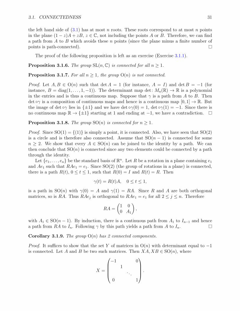
Proposition 3.1.7. For all n ≥ 1, the group O(n) is not connected.
Proof. Let A,B ∈ O(n) such that detA = 1 (for instance, A = I) and detB = −1 (forinstance, B = diag(1, . . . , 1,−1)). The determinant map det : Mn(R) → R is a polynomialin the entries and is thus a continuous map. Suppose that γ is a path from A to B. Thendet ◦γ is a composition of continuous maps and hence is a continuous map [0, 1] → R. Butthe image of det ◦γ lies in {±1} and we have det ◦γ(0) = 1, det ◦γ(1) = −1. Since there isno continuous map R→ {±1} starting at 1 and ending at −1, we have a contradiction.
Proposition 3.1.8. The group SO(n) is connected for n ≥ 1.
Proof. Since SO(1) = {(1)} is simply a point, it is connected. Also, we have seen that SO(2)is a circle and is therefore also connected. Assume that SO(n − 1) is connected for somen ≥ 2. We show that every A ∈ SO(n) can be joined to the identity by a path. We canthen conclude that SO(n) is connected since any two elements could be connected by a paththrough the identity.
Let {e1, . . . , en} be the standard basis of Rn. Let R be a rotation in a plane containing e1
and Ae1 such that RAe1 = e1. Since SO(2) (the group of rotations in a plane) is connected,there is a path R(t), 0 ≤ t ≤ 1, such that R(0) = I and R(t) = R. Then
γ(t) = R(t)A, 0 ≤ t ≤ 1,
is a path in SO(n) with γ(0) = A and γ(1) = RA. Since R and A are both orthogonalmatrices, so is RA. Thus RAej is orthogonal to RAe1 = e1 for all 2 ≤ j ≤ n. Therefore
RA =
(1 00 A1
),
with A1 ∈ SO(n − 1). By induction, there is a continuous path from A1 to In−1 and hencea path from RA to In. Following γ by this path yields a path from A to In.
Corollary 3.1.9. The group O(n) has 2 connected components.
Proof. It suffices to show that the set Y of matrices in O(n) with determinant equal to −1is connected. Let A and B be two such matrices. Then XA,XB ∈ SO(n), where
X =
−1 0
1. . .
0 1
.
32 CHAPTER 3. TOPOLOGY OF LIE GROUPS
Since SO(n) is connected, there is a path γ : [0, 1]→ SO(n) with γ(0) = XA and γ(1) = XB.Then Xγ(t) is a path from A to B in Y .
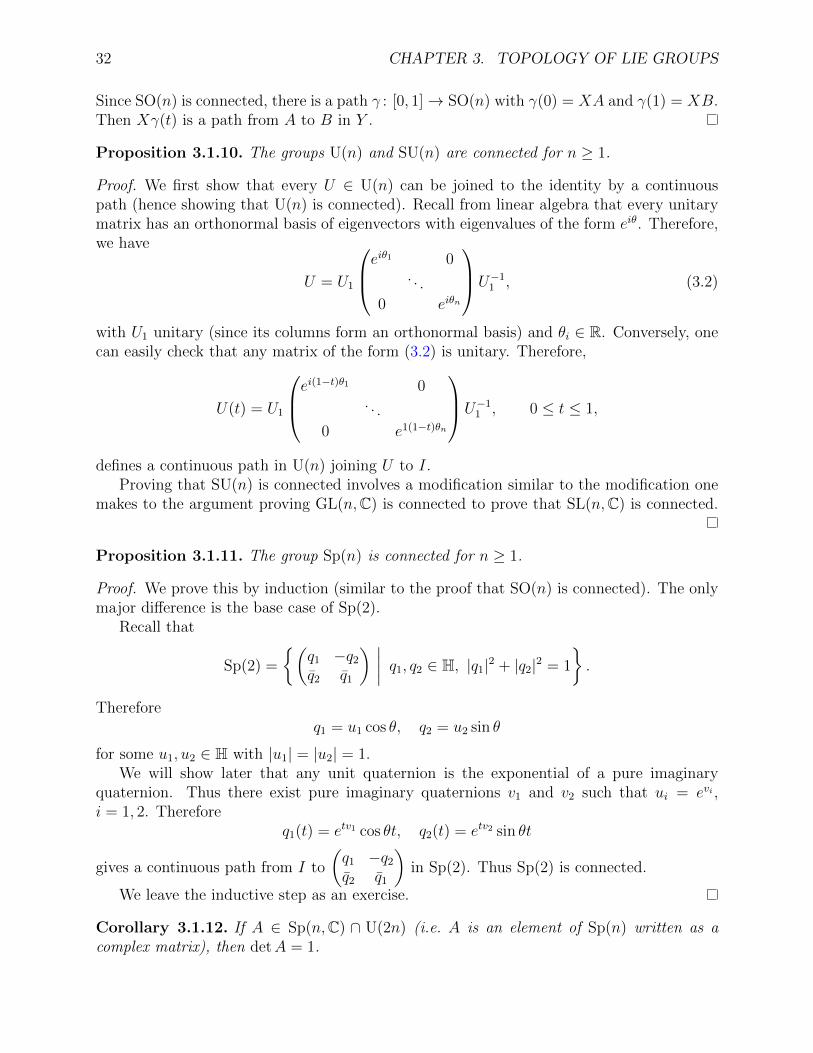
Proposition 3.1.10. The groups U(n) and SU(n) are connected for n ≥ 1.
Proof. We first show that every U ∈ U(n) can be joined to the identity by a continuouspath (hence showing that U(n) is connected). Recall from linear algebra that every unitarymatrix has an orthonormal basis of eigenvectors with eigenvalues of the form eiθ. Therefore,we have
U = U1
eiθ1 0
. . .
0 eiθn
U−11 , (3.2)
with U1 unitary (since its columns form an orthonormal basis) and θi ∈ R. Conversely, onecan easily check that any matrix of the form (3.2) is unitary. Therefore,
U(t) = U1
ei(1−t)θ1 0
. . .
0 e1(1−t)θn
U−11 , 0 ≤ t ≤ 1,
defines a continuous path in U(n) joining U to I.Proving that SU(n) is connected involves a modification similar to the modification one
makes to the argument proving GL(n,C) is connected to prove that SL(n,C) is connected.
Proposition 3.1.11. The group Sp(n) is connected for n ≥ 1.
Proof. We prove this by induction (similar to the proof that SO(n) is connected). The onlymajor difference is the base case of Sp(2).
Recall that
Sp(2) =
{(q1 −q2
q2 q1
) ∣∣∣∣ q1, q2 ∈ H, |q1|2 + |q2|2 = 1
}.
Thereforeq1 = u1 cos θ, q2 = u2 sin θ
for some u1, u2 ∈ H with |u1| = |u2| = 1.We will show later that any unit quaternion is the exponential of a pure imaginary
quaternion. Thus there exist pure imaginary quaternions v1 and v2 such that ui = evi ,i = 1, 2. Therefore
q1(t) = etv1 cos θt, q2(t) = etv2 sin θt
gives a continuous path from I to
(q1 −q2
q2 q1
)in Sp(2). Thus Sp(2) is connected.
We leave the inductive step as an exercise.
Corollary 3.1.12. If A ∈ Sp(n,C) ∩ U(2n) (i.e. A is an element of Sp(n) written as acomplex matrix), then detA = 1.
3.2. POLAR DECOMPOSITIONS 33
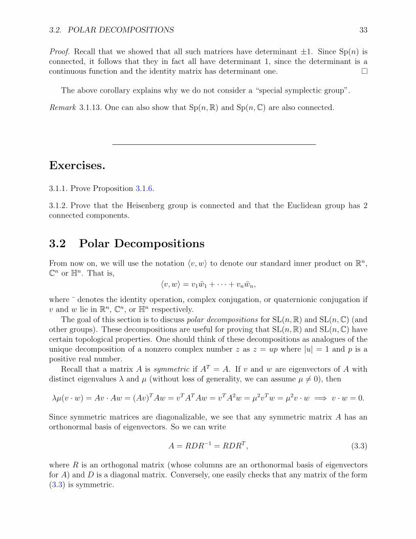
Proof. Recall that we showed that all such matrices have determinant ±1. Since Sp(n) isconnected, it follows that they in fact all have determinant 1, since the determinant is acontinuous function and the identity matrix has determinant one.
The above corollary explains why we do not consider a “special symplectic group”.
Remark 3.1.13. One can also show that Sp(n,R) and Sp(n,C) are also connected.
Exercises.
3.1.1. Prove Proposition 3.1.6.
3.1.2. Prove that the Heisenberg group is connected and that the Euclidean group has 2connected components.
3.2 Polar Decompositions
From now on, we will use the notation 〈v, w〉 to denote our standard inner product on Rn,Cn or Hn. That is,
〈v, w〉 = v1w1 + · · ·+ vnwn,
where ¯ denotes the identity operation, complex conjugation, or quaternionic conjugation ifv and w lie in Rn, Cn, or Hn respectively.
The goal of this section is to discuss polar decompositions for SL(n,R) and SL(n,C) (andother groups). These decompositions are useful for proving that SL(n,R) and SL(n,C) havecertain topological properties. One should think of these decompositions as analogues of theunique decomposition of a nonzero complex number z as z = up where |u| = 1 and p is apositive real number.
Recall that a matrix A is symmetric if AT = A. If v and w are eigenvectors of A withdistinct eigenvalues λ and µ (without loss of generality, we can assume µ 6= 0), then
λµ(v · w) = Av · Aw = (Av)TAw = vTATAw = vTA2w = µ2vTw = µ2v · w =⇒ v · w = 0.
Since symmetric matrices are diagonalizable, we see that any symmetric matrix A has anorthonormal basis of eigenvectors. So we can write
A = RDR−1 = RDRT , (3.3)
where R is an orthogonal matrix (whose columns are an orthonormal basis of eigenvectorsfor A) and D is a diagonal matrix. Conversely, one easily checks that any matrix of the form(3.3) is symmetric.
34 CHAPTER 3. TOPOLOGY OF LIE GROUPS
Definition 3.2.1 (Positive real symmetric matrix). An n × n real symmetric matrix P ispositive (or positive-definite) if 〈x, Px〉 > 0 for all nonzero vectors x ∈ Rn. Equivalently, areal symmetric matrix is positive if all of its eigenvalues are positive.
By the above, given a real symmetric positive matrix P , there exists an orthogonal matrixR such that
P = RDR−1,
where D is diagonal with positive diagonal entries λ1, . . . , λn. We can then construct a squareroot of P as
P 1/2 = RD1/2R−1, (3.4)
where D is the diagonal matrix with positive diagonal entries λ1/21 , . . . , λ
1/2n . So P 1/2 is also
symmetric and positive. In fact, one can show that P 1/2 is the unique positive symmetricmatrix whose square is P (Exercise 3.2.1).
Proposition 3.2.2 (Polar decomposition of SL(n,R)). For every A ∈ SL(n,R), there existsa unique pair (R,P ) such that R ∈ SO(n), P is real, symmetric and positive, and A = RP .The matrix P satisfies detP = 1.
Proof. If such a pair existed, we would have
ATA = (RP )T (RP ) = P TRTRP = PIP = P 2.
Since (ATA)T = AT (AT )T = ATA, the matrix ATA is symmetric. It is also positive sincefor all x ∈ Rn, x 6= 0, we have
〈x,ATAx〉 = 〈Ax,Ax〉 > 0
since Ax 6= 0 (because A is invertible). Therefore we can define
P = (ATA)1/2,
and this P is real, symmetric, and positive. Since we want A = RP , we define
R = AP−1 = A((ATA)1/2)−1.
For the existence part of the proposition, it remains to show that R ∈ SO(n). Since
RTR = A((ATA)1/2)−1((ATA)1/2)−1AT (recall that ATA is symmetric)
= A(ATA)−1AT = AA−1(AT )−1AT = I,
we see that R ∈ O(n). Also, we have
1 = detA = detR detP.
Since P is positive (in particular, all its eigenvalues are positive), we have detP > 0. There-fore, detR > 0 and so detR = 1 (since R is orthogonal, detR = ±1). It then follows thatdetP = 1 as well.
To prove uniqueness, note that we saw above that we must have P 2 = ATA. By theuniqueness of the square root of a real, symmetric, positive matrix, P is unique. ThenR = AP−1 is also unique.
3.2. POLAR DECOMPOSITIONS 35
Definition 3.2.3 (Positive self-adjoint complex matrix). If P is an n × n self-adjoint (orhermitian) complex matrix (i.e. P ∗ = P ), then we say P is positive (or positive-definite) if〈x, Px〉 > 0 for all nonzero x ∈ Cn.
Proposition 3.2.4 (Polar decomposition of SL(n,C)). For every A ∈ SL(n,C), there existsa unique pair (U, P ) with U ∈ SU(n), P self-adjoint and positive, and A = UP . The matrixP satisfies detP = 1.
Proof. The proof is analogous to the proof of the polar decomposition for SL(n,R).
Remark 3.2.5. (a) Any complex matrix A can be written in the form A = UP where U isunitary and P is a positive-semidefinite (〈x,Ax〉 ≥ 0 for all x ∈ Cn) self-adjoint matrix.We just do not have the uniqueness statement in general.
(b) Our decomposition gives a polar decomposition
detA = detP detU = reiθ
of the determinant of A since detP is a nonnegative real number and detU is a unitcomplex number.
(c) We have similar (unique) polar decompositions for
GL(n,R), GL(n,R)+ = {A ∈ GL(n,R) | detA > 0}, and GL(n,C).
GL(n,R) : A = UP, U ∈ O(n), P real, symmetric, positive
GL(n,R)+ : A = UP, U ∈ SO(n), P real, symmetric, postive
GL(n,C) : A = UP, U ∈ U(n), P self-adjoint, positive
The proofs of these are left as an exercise. Note that the only difference between thepolar decomposition statements for GL(n,R)+ and SL(n,R) is that we do not concludethat detP = 1 for GL(n,R)+.
Exercises.
3.2.1. Show that P 1/2 given by (3.4) is the unique positive symmetric matrix whose squareis P . Hint: show that any matrix that squares to P has the same set of eigenvectors as P .
3.2.2. Prove the results stated in Remark 3.2.5(c).
3.2.3. Prove that a real symmetric matrix is positive if and only if all of its eigenvalues arepositive (see Definition 3.2.1).
36 CHAPTER 3. TOPOLOGY OF LIE GROUPS
3.3 Compactness
Definition 3.3.1 (Comact). A matrix Lie group G is compact if the following two conditionsare satisfied:
(a) The set G is closed in Mn(C): If Am is a sequence of matrices in G, and Am convergesto a matrix A, then A is in G.
(b) The set G is bounded: There exists a constant C ∈ R such that for all A ∈ G, |Aij| ≤ Cfor all 1 ≤ i, j ≤ n.
Remark 3.3.2. (a) The conditions in the above definition say that G is a closed boundedsubset of Cn2
(when we identify Mn(C) with Cn2). For subsets of Cn2
, this is equivalentto the usual, more general, definition of compact (that any open cover has a finitesubcover).
(b) All of our examples of matrix Lie groups except GL(n,R) and GL(n,C) satisfy theclosure condition above. Thus, we are most interested in the boundedness condition.
Proposition 3.3.3. The groups O(n), SO(n), U(n), SU(n) and Sp(n) are compact.
Proof. We have already noted that these groups satisfy the closure condition. The columnvectors of any matrix in the first four groups in the proposition have norm one (and also inthe last if we consider the complex form of elements of Sp(n)) and hence |Aij| ≤ 1 for all1 ≤ i, j ≤ n.
Proposition 3.3.4. The following groups are noncompact:
GL(n,R), GL(n,C), n ≥ 1,
SL(n,R), SL(n,C), O(n,C), SO(n,C), n ≥ 2,
H, Sp(n,R), Sp(n,C), E(n), Rn, R∗, C∗, n ≥ 1.
Proof. The groups GL(n,R) and GL(n,C) violate the closure condition since a limit ofinvertible matrices may be not invertible.
Since a
1a
1. . .
1
has determinant one for any nonzero a, we see that the groups SL(n,R) and SL(n,C) arenot bounded for n ≥ 2.
We have (z −ww z
)∈ SO(2,C)
for z, w ∈ C with z2 + w2 = 1. We can take z with |z| arbitrarily large and let w be anysolution to z2 + w2 = 1 (such solutions always exist over the complex numbers) and thus
3.4. LIE GROUPS 37
SO(2) is unbounded. By considering block matrices, we see that SO(n) is unbounded forn ≥ 2.
We leave the remaining cases as an exercise (Exercise 3.3.1).
Exercises.
3.3.1. Complete the proof of Proposition 3.3.4.
3.4 Lie groups
Technically speaking, we gave the definition of an arbitrary Lie group (as opposed to amatrix Lie group) in Section 1.1. But in this section we will give the definition more directly.Although we will focus on matrix Lie groups in this course, it is useful to see the more generaldefinition, which is the approach one must take if one wishes to study Lie groups in moredetail (beyond this course). Our discussion here will be very brief. Further details can befound in [Hal03, Appendix C].
Definition 3.4.1 (Lie group). A (real) Lie group is a (real) smooth manifold G which isalso a group and such that the group product G×G→ G and the inverse map g 7→ g−1 aresmooth maps.
Roughly speaking, a smooth manifold is an object that looks locally like Rn. For example,the torus is a two-dimensional manifold since it looks locally (but not globally) like R2.
Example 3.4.2. Let
G = R× R× S1,
with group product
(x1, y1, u1) · (x2, y2, u2) = (x1 + x2, y1 + y2, eix1y2u1u2).
One can check that this operation does indeed make G into a group (Exercise 3.4.1). Themultiplication and inversion maps are both smooth, and so G is a Lie group. However, onecan show that G is not isomorphic to a matrix Lie group (see [Hal03, §C.3]).
Theorem 3.4.3 ([Sti08, Corollary 2.33]). Every matrix Lie group is a smooth embeddedsubmanifold of Mn(C) and is thus a Lie group.
Usually one says that a map Φ between Lie groups is a Lie group homomorphism if Φis a group homomorphism and Φ is smooth. However, in Definition 2.11.1, we only requiredthat Φ be continuous. This is because of the following result. A proof for the case of matrixLie groups can be found in [Sti08, Corollary 2.34].
38 CHAPTER 3. TOPOLOGY OF LIE GROUPS
Proposition 3.4.4. Suppose G and H are Lie groups and Φ: G→ H is a group homomor-phism from G to H. If Φ is continuous, then it is also smooth.
Exercises.
3.4.1. Show that G, as defined in Example 3.4.2, is a group.
Chapter 4
Maximal tori and centres
From now on, we will sometimes use the term Lie group. For the purposes of this course,you can replace this term by matrix Lie group. In this chapter we discuss some importantsubgroups of Lie groups.
4.1 Maximal tori
Definition 4.1.1 (Torus). A torus (or k-dimensional torus) is a group isomorphic to
Tk = S1 × S1 × · · · × S1 (k-fold Cartesian product).
A maximal torus of a Lie group G is a torus subgroup T of G such that if T ′ is another torussubgroup containing T then T = T ′.
Remark 4.1.2. (a) Note that tori are abelian.
(b) For those who know something about Lie algebras, maximal tori correspond to Cartansubalgebras of Lie algebras.
Example 4.1.3. The group SO(2) = S1 = T1 is its own maximal torus.
Recall that SO(3) is the group of rotations of R3. Let e1, e2, e3 be the standard basisvectors. Then the matrices
R′θ =
cos θ − sin θ 0sin θ cos θ 0
0 0 1
=
(Rθ 00 1
), θ ∈ R,
form a copy of T1 in SO(3).
Proposition 4.1.4. The set {R′θ | θ ∈ R} forms a maximal torus in SO(3).
Proof. Suppose T is a torus in SO(3) containing this T1. Since all tori are abelian, any A ∈ Tcommutes with all R′θ ∈ T1. Thus is suffices to show that, for A ∈ SO(3),
AR′θ = R′θA for all R′θ ∈ T1 (4.1)
39
40 CHAPTER 4. MAXIMAL TORI AND CENTRES
implies that A ∈ T1. Suppose A ∈ SO(3) satisfies (4.1). First we show that
A(e1), A(e2) ∈ Span{e1, e2}.
SupposeA(e1) = a1e1 + a2e2 + a3e3.
By (4.1), A commutes with
R′π =
−1 0 00 −1 00 0 1
.
Since
AR′π(e1) = A(−e1) = −a1e1 − a2e2 − a3e3,
R′πA(e1) = R′π(a1e1 + a2e2 + a3e3) = −a1e1 − a2e2 + a3e3,
we have a3 = 0 and so A(e1) ∈ Span{e1, e2} as desired. A similar argument shows thatA(e2) ∈ Span{e1, e2}.
Thus, the restriction of A to the (e1, e2)-plane is an isometry of that plane that fixesthe origin. Therefore it is a rotation or a reflection. However, no reflection commutes withall rotations (Exercise 4.1.1). Thus A must be a rotation in the (e1, e2)-plane. Since Apreserves the dot product, it must leave invariant Re3, which is the orthogonal complementto Span{e1, e2}. So A is of the form
A =
(Rθ 00 c
)for some c ∈ R. Since detA = detRθ = 1, it follows that c = 1, and hence A ∈ T1 asdesired.
Definition 4.1.5 (Centre). The centre of a Lie group G is the subgroup (see Exercise 4.1.2)
Z(G) = {A ∈ G | AB = BA ∀ B ∈ G}.
Corollary 4.1.6. The Lie group SO(3) has trivial centre:
Z(SO(3)) = {1}.
Proof. Suppose A ∈ Z(SO(3)). Then A commutes with all elements of SO(3) and hence allelements of T1. By the above argument, this implies that A fixes e3. Interchanging basisvectors in this argument shows that A also fixes e1 and e2 and hence A is the identity.
We now find maximal tori in all of the compact connected matrix Lie groups we haveseen. We focus on connected groups because one can easily see (since Tk is connected) thata maximal torus must always be contained in the identity component of a Lie group.
First of all, we note that there are at least three natural matrix groups isomorphic to T1:
(a) The group {Rθ | θ ∈ R} consisting of 2× 2 matrices.
4.1. MAXIMAL TORI 41
(b) The groupeiθ = cos θ + i sin θ, θ ∈ R,
consisting of complex numbers (or 1× 1 complex matrices).
(c) The groupeiθ = cos θ + i sin θ, θ ∈ R,
consisting of quaternions (or 1× 1 quaternionic matrices).
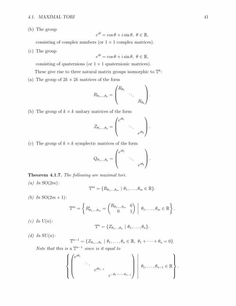
These give rise to three natural matrix groups isomorphic to Tk:
(a) The group of 2k × 2k matrices of the form
Rθ1,...,θk =
Rθ1. . .
Rθk
.
(b) The group of k × k unitary matrices of the form
Zθ1,...,θk =
eiθ1
. . .
eiθk
.
(c) The group of k × k symplectic matrices of the form
Qθ1,...,θk =
eiθ1
. . .
eiθk
.
Theorem 4.1.7. The following are maximal tori.
(a) In SO(2m):Tm = {Rθ1,...,θm | θ1, . . . , θm ∈ R}.
(b) In SO(2m+ 1):
Tm =
{R′θ1,...,θm =
(Rθ1,...,θm 0
0 1
) ∣∣∣∣ θ1, . . . , θm ∈ R}.
(c) In U(n):Tn = {Zθ1,...,θn | θ1, . . . , θn}.
(d) In SU(n):Tn−1 = {Zθ1,...,θn | θ1, . . . , θn ∈ R, θ1 + · · ·+ θn = 0}.
Note that this is a Tn−1 since is it equal toeiθ1
. . .
eiθn−1
e−θ1−···−θn−1
∣∣∣∣∣∣∣∣∣ θ1, . . . , θn−1 ∈ R
.

42 CHAPTER 4. MAXIMAL TORI AND CENTRES
(e) In Sp(n):Tn = {Qθ1,...,θn | θ1, . . . , θn ∈ R}.
Proof. We prove each case separately. As for the case of SO(3) dealt with above, in each casewe will show that if an element A of the group commutes with all elements of the indicatedtorus, then A must be included in this torus. Then the result follows as it did for SO(3).
(a) Let e1, e2, . . . , e2m denote the standard basis of R2m. Suppose that A ∈ SO(2m)commutes will all elements of Tm. We first show that
A(e1), A(e2) ∈ Span{e1, e2},A(e3), A(e4) ∈ Span{e3, e4},
...
A(e2m−1), A(e2m) ∈ Span{e2m−1, e2m}.
We do the case of e1, since the rest are analogous. Recall that we assume that A commuteswith all elements of Tm. Therefore,
ARπ,0,...,0(e1) = Rπ,0,...,0A(e1).
IfA(e1) = a1e1 + · · ·+ a2me2m,
thenARπ,0,...,0(e1) = A(−e1) = −a1e1 − · · · − a2me2m,
but
Rπ,0,...,0A(e1) = Rπ,0,...,0(a1e1 + · · ·+ a2me2m) = −a1e1 − a2e2 + a3e3 + · · ·+ e2me2m.
Thusa3 = a4 = · · · = a2m
as desired. Therefore, A is a product of rotations or reflections in the planes
Span{e1, e2}, . . . , Span{e2m−1, e2m}.
However, the case of reflections is ruled out as it was for SO(3) and hence A is a product ofrotations in these planes and therefore is an element of Tm.
(b) This is a generalization of the argument for SO(3), using maps such as R′π,0,...,0 inplace of R′π. The details are left as an exercise.
(c) Let e1, . . . , en be the standard basis of Cn. Suppose that A ∈ U(n) commutes withall elements of Tn. In particular, A commutes with Zπ,0,...,0. Let
A(e1) = a1e1 + · · ·+ anen.
Then
AZπ,0,...,0(e1) = A(−e1) = −a1e1 − · · · − anen,Zπ,0,...,0A(e1) = Zπ,0,...,0(a1e1 + · · ·+ anen) = −a1e1 + a2e2 + · · ·+ anen.
Thus a2 = · · · = an = 0 and so A(e1) = c1e1 for some c1 ∈ C. A similar argument showsthat A(ek) = ckek for each k. Since A is unitary, we must have |ck| = 1 for each k and thusA ∈ Tn.
4.1. MAXIMAL TORI 43
(d) The case n = 1 is trivial and so we begin with the case n = 2. Suppose that
A =
(a bc d
)commutes will all elements of T1. Then A commutes with
Zπ/2,−π/2 =
(i 00 −i
),
and thus (ai −bici −di
)= AZπ/2,−π/2 = Zπ/2,−π/2A =
(ai bi−ci −di
).
Therefore b = c = 0. Then we must have |a| = |d| = 1 since A is unitary and a = d−1 sinceA has determinant one. Therefore A ∈ T1. For n > 2, we leave it as an exercise to showthat if A ∈ SU(n) commutes with Zπ,π,0,...,0 and Zπ,0,π,0,...,0 then Ae1 = c1e1 for some c1 ∈ C.(Note that we could not use Zπ,0,...,0 as we did for the U(n) case since detZπ,0,...,0 = −1.)Similarly, one can show that Aek = ckek for each k. Then the result follows as it did for theU(n) case.
(e) Suppose A ∈ Sp(n) commutes with all elements of Tn. By the argument used forU(n), one can show that for all k, Aek = ckek for some ck ∈ H. But then the fact that Amust commute with all elements of Tn shows that each ck must commute with all eiθ, θ ∈ R.In particular, ck must commute with i and thus ck ∈ R + Ri. We must also have |ck| = 1since A ∈ Sp(n) and so A ∈ Tn.
Remark 4.1.8. (a) Note that in our proofs, we only used the fact that A commuted withall elements of the torus in question. Thus it follows that these maximal tori are alsomaximal abelian subgroups of the respective Lie groups.
(b) Since Tk is connected, any maximal torus must lie in the identity component of the Liegroup. Therefore, the maximal tori of SO(2m) and SO(2m + 1) found above are alsomaximal tori of O(2m) and O(2m+ 1).
Remark 4.1.9. A noncompact Lie group need not have any nontrivial tori (for example, Rn).However, the maximal tori in compact groups are well-behaved. In particular, we have thefollowing results which we state without proof (at least for now) because the proofs usematerial we have not covered. They are useful facts that motivate some of the terminologywe will use. Let G be a compact Lie group and T a maximal torus.
(a) Every conjugate of a maximal torus is a maximal torus.
(b) Every element g ∈ G is conjugate to an element of T , hence lies in a maximal torus.
(c) All maximal tori in G are conjugate. So the maximal tori form a single conjugacy classin G.
(d) It follows that all maximal tori in G have the same dimension, called the rank of G.
44 CHAPTER 4. MAXIMAL TORI AND CENTRES
Exercises.
4.1.1. Show that no reflection of the plane commutes with all rotations.
4.1.2. Show that Z(G) is indeed a subgroup of G. In fact, show that it is a Lie subgroup ofG.
4.2 Centres
We now determine the centres of the compact classical groups SO(n), U(n), SU(n) and Sp(n).Any element of the centre of a Lie groups commutes will all elements of the Lie group andthus with all elements of a maximal torus. Therefore, by the arguments of the previoussection, the centres are contained in the maximal tori we described there. Note also thatany scalar multiple of the identity n× n matrix commutes will all n× n matrices.
Theorem 4.2.1. The compact classical groups have the following centres.
(a) Z(SO(2)) = SO(2), Z(SO(2m)) = {±1}, m ≥ 2.
(b) Z(SO(2m+ 1)) = {1}, m ≥ 1.
(c) Z(U(n)) = {ω1 | |ω| = 1}, n ≥ 1.
(d) Z(SU(n)) = {ω1 | ωn = 1}, n ≥ 1.
(e) Z(Sp(n)) = {±1}, n ≥ 1.
Here 1 = I is the identity matrix.
Proof. All of the subgroups mentioned in the proposition consist of multiples of the identitymatrix. Therefore, by the above comment, they are contained in the centres. It thus sufficesto show that all elements of the centres lie in these subgroups.
(a) We know that SO(2) is abelian and so the first statement follows. Suppose A ∈Z(SO(2m)), m ≥ 2. As noted, we can assume that A lies in the maximal torus Tm. ThusA = Rθ1,...,θm for some θ1, . . . , θm ∈ R. Let
M =
(1 00 −1
).
Then Rθ commutes with M if and only if(cos θ sin θsin θ − cos θ
)=
(cos θ − sin θsin θ cos θ
)M = M
(cos θ − sin θsin θ cos θ
)=
(cos θ − sin θ− sin θ − cos θ
).
So Rθ commutes with M if and only if sin θ = 0, which implies cos θ = ±1.
4.3. DISCRETE SUBGROUPS AND THE CENTRE 45
Forming a matrix with (an even number of) copies of M on the diagonal (and all otherentries zero), we see that A will commute with such matrices if and only if each sin θk = 0and cos θk = ±1. Therefore, A is a diagonal matrix with diagonal entries ±1. Suppose thatboth +1 and −1 occur. Then let B be the matrix with Rθ (with sin θ 6= 0) on the diagonalat the position of an adjacent +1 and −1 (and otherwise only 1’s on the diagonal). Then Adoes not commute with B. Therefore A = I or A = −I as desired.
(b) We follow the argument for SO(2m). However, since −I 6= SO(2m+ 1), we concludethat A = I.
(c) If n = 1, then U(n) is isomorphic to S1 = {eiθ | θ ∈ R}, which is abelian and thusU(1) is its own centre. Therefore we assume n ≥ 2. Let A ∈ Z(U(n)). Then A = Zθ1,...,θn
for some θ1, . . . , θn ∈ R. Note that
(0 ii 0
)∈ U(2) (in fact, it is in SU(2), something we will
use in the next part) and(0 ieiθ1
ieiθ2 0
)=
(eiθ1 00 eiθ2
)(0 ii 0
)=
(0 ii 0
)(eiθ1 00 eiθ2
)=
(0 ieiθ2
ieiθ1 0
)if and only if eiθ1 = eiθ2 . Therefore, since A must commute with all matrices obtained
by placing a
(0 ii 0
)somewhere on the diagonal, 1’s elsewhere on the diagonal, and zeros
everywhere else, we see that eiθ1 = · · · = eiθn . Therefore A = eiθ1I as desired.(d) Let A ∈ Z(SU(n)). The argument for U(n) shows that A = ωI for some ω ∈ C,
|w| = 1. We must also have1 = detA = ωn,
as claimed.
Note: [Sti08] uses the matrix
(0 11 0
)instead of
(0 ii 0
)for the proof of the U(n) and
SU(n) cases. While this works for U(n), it is a problem for SU(n) since this matrix does nothave determinant one.
(e) Let A ∈ Z(Sp(n)). An argument similar to the one used for U(n) shows that A = qIfor some q ∈ H with |q| = 1. However, since this matrix must commute with all elements ofSp(n), it must, in particular, commute with I, iI, jI and kI. Thus, q must commute withall quaternions. But the only quaternions that commute with all other quaternions are thereal numbers. Thus q ∈ R. But then |q| = 1 implies that q = ±1 as desired.
4.3 Discrete subgroups and the centre
Recall that a subgroup H of a group G is normal if
gHg−1 = H for all g ∈ G,
and G is simple if it has no nontrivial (i.e. not equal to {1} or G) normal subgroups. It iseasy to see that the centre Z(G) of a group G is a normal subgroup of G. Thus if G hasnontrivial centre, it is not simple. Therefore, by our computation of centres in the previous
46 CHAPTER 4. MAXIMAL TORI AND CENTRES
section, the groups SO(2m), U(n), SU(n) and Sp(n) are not simple. This leaves SO(2m+ 1)as the only possibility.
Given any two matrices A,B ∈ Mn(C), we can consider the distance between them aspoints in Cn2
. Thus, the distance d(A,B) between A and B is√ ∑1≤i,j≤n
|aij − bij|2.
Definition 4.3.1 (Discrete subgroup). A subgroup H of a Lie group G is called discrete ifthere is a positive lower bound to the distance between any two distinct elements of H. Inother words H is discrete if there exists a c > 0 such that
d(A,B) > c for all A,B ∈ H, A 6= B.
It follows immediately that any finite subgroup of G is discrete – just take c to be theminimum of the (finite number of) distances between elements of H. Thus, the centres ofSO(n), SU(n), and Sp(n) are discrete. However, the centre of U(n) is not.
Theorem 4.3.2 (Schreier’s Theorem). If G is a path-connected Lie group then any discretenormal subgroup is contained in the centre of G.
Proof. Let H be a discrete normal subgroup of G. Then
BAB−1 ∈ H for all A ∈ H, B ∈ G.
Fix A ∈ H. Then we have a continuous map
ϕ : G→ H, ϕ(B) = BAB−1.
Note that ϕ(1) = A. Let C be an arbitrary element of G. Since G is path-connected, thereis a path from 1 to C. Since ϕ is continuous, it maps this path to a path in H. But H isdiscrete and so the image must be the single point A. In other words ϕB = BAB−1 = A orBA = AB for all B ∈ G. Therefore A ∈ Z(G). So H ⊆ Z(G).
We have seen that SO(n), SU(n), and Sp(n) are all path-connected. Therefore, their dis-crete normal subgroups are contained in their centres, which we have computed. Conversely,any subgroup of the centre is normal and so, in fact, we now know all the discrete normalsubgroups of these Lie groups. In particular, since Z(SO(2m + 1)) = {1}, the Lie groupSO(2m+ 1) has no nontrivial discrete normal subgroups.
We will see later that there are no normal subgroups of these Lie groups that are notdiscrete. In particular, it will follow that SO(2m+1) is simple and that the others are simplemodulo their centres (i.e. G/Z(G) is simple).
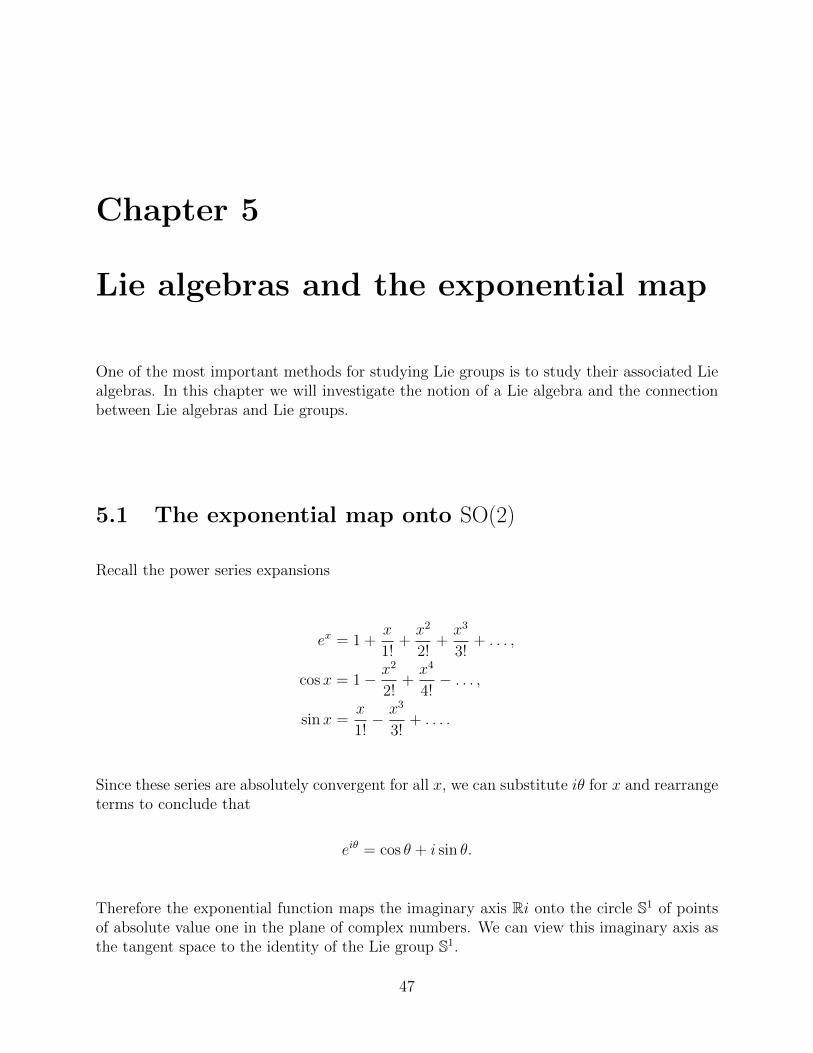
Chapter 5
Lie algebras and the exponential map
One of the most important methods for studying Lie groups is to study their associated Liealgebras. In this chapter we will investigate the notion of a Lie algebra and the connectionbetween Lie algebras and Lie groups.
5.1 The exponential map onto SO(2)
Recall the power series expansions
ex = 1 +x
1!+x2
2!+x3
3!+ . . . ,
cosx = 1− x2
2!+x4
4!− . . . ,
sinx =x
1!− x3
3!+ . . . .
Since these series are absolutely convergent for all x, we can substitute iθ for x and rearrangeterms to conclude that
eiθ = cos θ + i sin θ.
Therefore the exponential function maps the imaginary axis Ri onto the circle S1 of pointsof absolute value one in the plane of complex numbers. We can view this imaginary axis asthe tangent space to the identity of the Lie group S1.
47
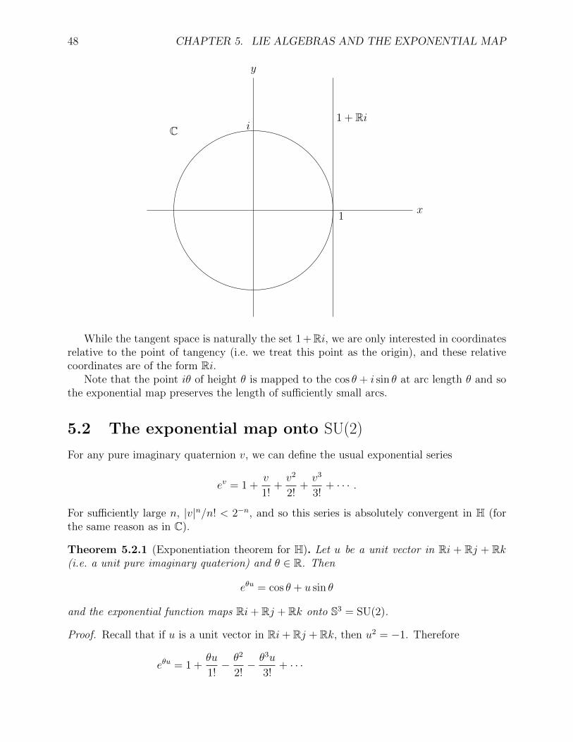
48 CHAPTER 5. LIE ALGEBRAS AND THE EXPONENTIAL MAP
x
y
i
1
1 + RiC
While the tangent space is naturally the set 1 +Ri, we are only interested in coordinatesrelative to the point of tangency (i.e. we treat this point as the origin), and these relativecoordinates are of the form Ri.
Note that the point iθ of height θ is mapped to the cos θ + i sin θ at arc length θ and sothe exponential map preserves the length of sufficiently small arcs.
5.2 The exponential map onto SU(2)
For any pure imaginary quaternion v, we can define the usual exponential series
ev = 1 +v
1!+v2
2!+v3
3!+ · · · .
For sufficiently large n, |v|n/n! < 2−n, and so this series is absolutely convergent in H (forthe same reason as in C).
Theorem 5.2.1 (Exponentiation theorem for H). Let u be a unit vector in Ri + Rj + Rk(i.e. a unit pure imaginary quaterion) and θ ∈ R. Then
eθu = cos θ + u sin θ
and the exponential function maps Ri+ Rj + Rk onto S3 = SU(2).
Proof. Recall that if u is a unit vector in Ri+ Rj + Rk, then u2 = −1. Therefore
eθu = 1 +θu
1!− θ2
2!− θ3u
3!+ · · ·
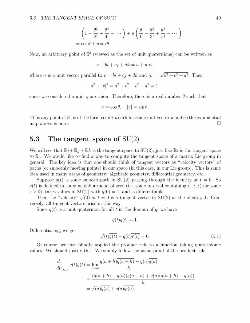
5.3. THE TANGENT SPACE OF SU(2) 49
=
(1− θ2
2!+θ4
4!− · · ·
)+ u
(θ
1!− θ3
3!+θ5
5!− · · ·
)= cos θ + u sin θ.
Now, an arbitrary point of S3 (viewed as the set of unit quaternions) can be written as
a+ bi+ cj + dk = a+ u|v|,
where u is a unit vector parallel to v = bi+ cj + dk and |v| =√b2 + c2 + d2. Then
a2 + |v|2 = a2 + b2 + c2 + d2 = 1,
since we considered a unit quaternion. Therefore, there is a real number θ such that
a = cos θ, |v| = sin θ.
Thus any point of S3 is of the form cos θ+u sin θ for some unit vector u and so the exponentialmap above is onto.
5.3 The tangent space of SU(2)
We will see that Ri+Rj+Rk is the tangent space to SU(2), just like Ri is the tangent spaceto S1. We would like to find a way to compute the tangent space of a matrix Lie group ingeneral. The key idea is that one should think of tangent vectors as “velocity vectors” ofpaths (or smoothly moving points) in our space (in this case, in our Lie group). This is sameidea used in many areas of geometry: algebraic geometry, differential geometry, etc.
Suppose q(t) is some smooth path in SU(2) passing through the identity at t = 0. Soq(t) is defined in some neighbourhood of zero (i.e. some interval containing (−ε, ε) for someε > 0), takes values in SU(2) with q(0) = 1, and is differentiable.
Then the “velocity” q′(0) at t = 0 is a tangent vector to SU(2) at the identity 1. Con-versely, all tangent vectors arise in this way.
Since q(t) is a unit quaternion for all t in the domain of q, we have
q(t)q(t) = 1.
Differentiating, we getq′(t)q(t) + q(t)q′(t) = 0. (5.1)
Of course, we just blindly applied the product rule to a function taking quaternionicvalues. We should justify this. We simply follow the usual proof of the product rule:
d
dt
∣∣∣∣t=a
q(t)q(t) = limh→0
q(a+ h)q(a+ h)− q(a)q(a)
h
=(q(a+ h)− q(a))q(a+ h) + q(a)(q(a+ h)− q(a))
h
= q′(a)q(a) + q(a)q′(a).
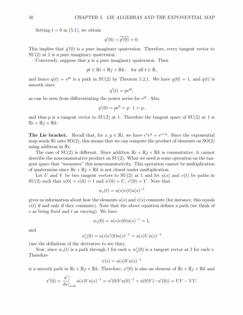
50 CHAPTER 5. LIE ALGEBRAS AND THE EXPONENTIAL MAP
Setting t = 0 in (5.1), we obtain
q′(0) + q′(0) = 0.
This implies that q′(0) is a pure imaginary quaternion. Therefore, every tangent vector toSU(2) at 1 is a pure imaginary quaternion.
Conversely, suppose that p is a pure imaginary quaternion. Then
pt ∈ Ri+ Rj + Rk, for all t ∈ R,
and hence q(t) = ept is a path in SU(2) by Theorem 5.2.1. We have q(0) = 1, and q(t) issmooth since
q′(t) = pept,
as can be seen from differentiating the power series for ept. Also,
q′(0) = pe0 = p · 1 = p,
and thus p is a tangent vector to SU(2) at 1. Therefore the tangent space of SU(2) at 1 isRi+ Rj + Rk.
The Lie bracket. Recall that, for x, y ∈ Ri, we have exey = ex+y. Since the exponentialmap sends Ri onto SO(2), this means that we can compute the product of elements on SO(2)using addition in Ri.
The case of SU(2) is different. Since addition Ri + Rj + Rk is commutative, it cannotdescribe the noncommutative product on SU(2). What we need is some operation on the tan-gent space that “measures” this noncommutativity. This operation cannot be multiplicationof quaternions since Ri+ Rj + Rk is not closed under multiplication.
Let U and V be two tangent vectors to SU(2) at 1 and let u(s) and v(t) be paths inSU(2) such that u(0) = v(0) = 1 and u′(0) = U , v′(0) = V . Note that
ws(t) = u(s)v(t)u(s)−1
gives us information about how the elements u(s) and v(s) commute (for instance, this equalsv(t) if and only if they commute). Note that the above equation defines a path (we think ofs as being fixed and t as varying). We have
ws(0) = u(s)v(0)u(s)−1 = 1,
andw′s(0) = u(s)v′(0)u(s)−1 = u(s)V u(s)−1
(use the definition of the derivative to see this).Now, since ws(t) is a path through 1 for each s, w′s(0) is a tangent vector at 1 for each s.
Thereforex(s) = u(s)V u(s)−1
is a smooth path in Ri+ Rj + Rk. Therefore, x′(0) is also an element of Ri+ Rj + Rk and
x′(0) =d
ds
∣∣∣∣s=0
u(s)V u(s)−1 = u′(0)V u(0)−1 + u(0)V (−u′(0)) = UV − V U.
5.4. THE LIE ALGEBRA SU(2) OF SU(2) 51
Here we have used the fact that dds
∣∣s=0
u(s)−1 = −u′(0) if u(0) = 1 (see [Sti08, Exer-cise 4.3.2]).
We see that the map
(U, V ) 7→ [U, V ]
is a binary operation on the tangent space Ri + Rj + Rk to SU(2) at the identity, which isrelated to the (non)commutativity of SU(2).
5.4 The Lie algebra su(2) of SU(2)
Definition 5.4.1 (Lie algebra). A Lie algebra is a vector space g with a bilinear operation(the Lie bracket) [·, ·] : g× g→ g that
• is alternating : [X,X] = 0 for all X ∈ g (equivalently, if the field is not of characteristic2, [X, Y ] = −[Y,X] for all X, Y ∈ g), and
• satisfies the Jacobi identity
[X, [Y, Z]] + [Y, [Z,X]] + [Z, [X, Y ]] = 0.
If g1 and g2 are Lie algebras, a homomorphism (resp. isomorphism) of Lie algebras is alinear map (resp. vector space isomorphism) ϕ : g1 → g2 that commutes with the Lie bracket:
ϕ([X, Y ]1) = [ϕ(X), ϕ(Y )]2
where [·, ·]i denotes the Lie bracket on [·, ·]i, i = 1, 2.
Definition 5.4.2 (su(2)). It follows from Exercise 5.4.1 that Ri+Rj+Rk, with Lie bracketgiven by [U, V ] = UV −V U (i.e. the tangent space to SU(2) at the identity), is a Lie algebra.We denote this Lie algebra by su(2).
One can show that R3 is a Lie algebra with bracket equal to the cross-product (see [Sti08,Exercises 1.4.1 and 1.4.4]).
Definition 5.4.3 (Ideal of a Lie algebra). An ideal of a Lie algebra g is a subspace a of gwith the property that [X, Y ] ∈ a for all X ∈ g and Y ∈ a.
The proof of the following lemma is left as an exercise (Exercise 5.4.2).
Lemma 5.4.4. If ϕ : g1 → g2 is a homomorphism of Lie algebras, then kerϕ is an ideal ofg1.
The following notion will be useful for us later.
Definition 5.4.5 (Simple Lie algebra). A Lie algebra is simple if it has dimension at leasttwo and it has no proper nonzero ideals.
52 CHAPTER 5. LIE ALGEBRAS AND THE EXPONENTIAL MAP
Exercises.
5.4.1. Show that any vector space of matrices closed under matrix multiplication (moregenerally, any associative algebra) is a Lie algebra with bracket given by [A,B] = AB−BA.
5.4.2. Prove Lemma 5.4.4.
5.4.3. Show that Ri+ Rj + Rk (with Lie bracket as in Definition 5.4.2) is isomorphic to R3
with the cross-product. Note that the isomorphism is not given by the “identity” map.
5.5 The exponential of square matrices
Recall that we identify Mn(C) with Cn2or R2n2
and thus we have a matrix absolute value
‖A‖ =
√∑i,j
|aij|2, A = (aij).
This is the distance from the origin to the point A. Similarly, if A ∈ Mn(H), then ‖A‖ isthe distance from the origin to A in R4n2
(where we identify H with R4).If A,A1, A2, . . . are n× n matrices, we say
limm→∞
Am = A
if∀ ε ∃ M such that
(m > M =⇒ ‖Am − A‖ < ε
).
Equivalently, limm→∞Am = A if the limits of the entries of the Am exists and equal thecorresponding entries of A.
Proposition 5.5.1 (Submultiplicative property). If A and B are n× n real matrices, then‖AB‖ ≤ ‖A‖‖B‖.
Proof. Let A = (aij) and B = (bij) and C = AB = (cij). Then
|cij| = |ai1b1j + ai2b2j + · · ·+ ainbnj|= |(ai1, ai2, . . . , ain) · (b1j, b2j, . . . , bnj)|≤ |(ai1, ai2, . . . , ain)||(b1j, b2j, . . . , bnj)| (Cauchy-Schwartz Inequality).
Thus
‖AB‖2 =∑i,j
|cij|2
≤∑i,j
(|ai1|2 + · · ·+ |ain|2)(|bi1|2 + · · ·+ |bin|2)
5.5. THE EXPONENTIAL OF SQUARE MATRICES 53
=∑i
(|ai1|2 + · · ·+ |ain|2)∑j
(|bi1|2 + · · ·+ |bin|2)
= ‖A‖2‖B‖2.
Therefore ‖AB‖ ≤ ‖A‖‖B‖.
Proposition 5.5.2 (Convergence of the matrix exponential). If A is any real n× n matrix,then
In +A
1!+A2
2!+A3
3!+ · · · ,
is absolutely convergent in Rn2and hence defines a function of A. This function is continu-
ous.
Proof. The series
‖In‖+‖A‖1!
+‖A2‖
2!+‖A3‖
3!+ · · ·
is a series of positive real numbers, whose terms (except for the first) are less than or equalto the corresponding terms of
1 +‖A‖1!
+‖A‖2
2!+‖A‖3
3!+ · · ·
by the submultiplicative property. This is the power series for e‖A‖ and thus it converges.Therefore the series in the proposition converges absolutely.
Since each Am is continuous, the partial sums of the series are continuous. Since theseries converges uniformly (exercise) on every set of the form {A | ‖A‖ ≤ R}, R > 0, thesum is continuous.
Remark 5.5.3. Recall that complex numbers can be viewed as 2 × 2 real matrices, and onecan check that if Z is the matrix corresponding to the complex number z, then eZ is thematrix corresponding to the complex number ez. Thus, the exponential of a complex matrixmay be represented by the exponential of a real matrix and so the series above also convergesfor complex matrices. Similarly, it converges for quaternionic matrices.
Definition 5.5.4 (Exponential of a matrix). The exponential of an n×n (real, complex, orquaternionic) matrix A is
expA = eA = In +A
1!+A2
2!+A3
3!+ · · · .
Remark 5.5.5. One can define an exponential in the more general setting of Riemannianmanifolds, where it maps lines (through the origin) in the tangent space to geodesics throughthe tangent point. One can also define an exponential for arbitrary Lie groups by consideringone-parameter subgroups.
Proposition 5.5.6 (Properties of the matrix exponential). Suppose X and Y are arbitraryn× n (real, complex, or quaternionic) matrices. Then we have the following.
54 CHAPTER 5. LIE ALGEBRAS AND THE EXPONENTIAL MAP
(a) e0 = I.
(b) (eX)∗ = eX∗.
(c) eX is invertible and (eX)−1 = e−X .
(d) e(α+β)X = eαXeβX for all α and β in C.
(e) If XY = Y X, then eX+Y = eXeY = eY eX .
(f) If C is invertible, then eCXC−1
= CeXC−1.
(g) ‖eX‖ ≤ e‖X‖.
Proof. Part (a) is obvious. Part (b) follows by taking term-by-term adjoints (the adjoint ofa sum is the sum of adjoints and (Xm)∗ = (X∗)m). Parts (c) and (d) are special cases ofpart (e). For part (e), we compute
eXeY =
(I +X +
X2
2!+ · · ·
)(I + Y +
Y 2
2!+ · · ·
)=
∞∑m=0
m∑k=0
Xk
k!
Y m−k
(m− k)!=
∞∑m=0
1
m!
m∑k=0
m!
k!(m− k)!XkY m−k.
Now, when X and Y commute, we have
(X + Y )m =m∑k=0
m!
k!(m− k)!XkY m−k,
and so
eXeY =∞∑m=0
1
m!(X + Y )m = eX+Y .
Part (f) follows from the fact that (CXC−1)m = CXmC−1 and part (g) follows from ourproof of the convergence of the exponential of matrices.
Proposition 5.5.7. Let X be a square complex matrix. Then t 7→ etX is a smooth curve inMn(C) and
d
dtetX = XetX = etXX.
In particular,d
dtetX∣∣∣∣t=0
= X.
Proof. Since for each i, j, the entry (etX)ij is given by a convergent power series in t, we candifferentiate the series for etX term by term. The result follows easily.
At some points, we may wish to explicitly compute the exponential of a matrix X. Thereis a general method for doing this.
5.6. THE TANGENT SPACE 55
Case 1: X is diagonalizable. If X is diagonalizable, then there exists an invertiblematrix C such that X = CDC−1 with
D =
λ1 0. . .
0 λn
.
It is easy to check that
eD =
eλ1 0
. . .
0 eλn
,
and so, by Proposition 5.5.6, we have
eX = C
eλ1 0
0. . .
0 eλn
C−1,
Case 2: X is nilpotent. A matrix X is nilpotent if Xm = 0 for some m > 0 (henceX` = 0 for all ` > m). In this case the series for eX terminates after the first m terms andso can be computed explicitly. For example (an example related to the Heisenberg group),if
X =
0 a b0 0 c0 0 0
,
then
X2 =
0 0 ac0 0 00 0 0
,
and X3 = 0. Thus
eX =
1 a b+ ac/20 1 c0 0 1
.
General case: X arbitrary. By a theorem in linear algebra, every matrix X can bewritten uniquely in the form X = S+N , with S diagonalizable, N nilpotent, and SN = NS.Therefore,
eX = eS+N = eSeN ,
and we can compute eS and eN as in the previous cases.
5.6 The tangent space
Definition 5.6.1 (Smooth paths and their derivatives). Let S be a space of matrices. Wesay that a path t 7→ A(t) is smooth, or differentiable, if the coordinate functions aij(t) are
56 CHAPTER 5. LIE ALGEBRAS AND THE EXPONENTIAL MAP
differentiable. If A(t) is smooth, its derivative A′(t) is defined in the usual way by
lim∆t→0
A(t+ ∆t)− A(t)
∆t.
Remark 5.6.2. It follows from the definition that A′(t) is just the matrix with entries a′ij(t)where aij(t) are the entries of A(t).
Definition 5.6.3 (Tangent vectors and the tangent space). The tangent vectors at theidentity 1 of a matrix Lie group G are the matrices X of the form
X = A′(0)
where A(t) is a smooth path in G with A(0) = 1. The tangent space to G at 1 is the set ofall tangent vectors at 1.
Remark 5.6.4. We will see later (Proposition 5.10.1) that if X is a tangent vector at theidentity to a matrix Lie group G, then eX ∈ G. It follows that an equivalent definition ofthe tangent space is the set of all X such that etX ∈ G for all t ∈ R. (See Corollary 5.11.10and Remark 5.11.11.) In fact, this is the definition used in [Hal03] and it will be useful tosometimes use this characterization when computing tangent spaces.
Proposition 5.6.5 (Tangent spaces of O(n), U(n) and Sp(n)). The tangent spaces at theidentity of the groups O(n), U(n) and Sp(n) are given as follows.
(a) O(n): {X ∈Mn(R) | X +XT = 0}.
(b) U(n): {X ∈Mn(C) | X +X∗ = 0}.
(c) Sp(n): {X ∈Mn(H) | X +X∗ = 0}.
Proof. Let A(t) be a smooth path in O(n), U(n) or Sp(n) with A(0) = 1. Then
A(t)A(t)∗ = 1 for all t
(note that M∗ = MT for M ∈Mn(R)). Taking the derivative with respect to t, we obtain
A′(t)A(t)∗ + A(t)A′(t)∗ = 0.
(There are a few technicalities here, which are left as an exercise. For instance, one should
check that ddt
(MT ) = ( ddtM)T , d
dt
(A(t)
)= A′(t) – see Exercise 5.6.1.) Since A(0) = 1, we
haveA′(0) + A′(0)∗ = 0.
It follows that the tangent spaces are contained in the sets in the statement of the proposition.Now suppose that a matrix X satisfies X + X∗ = 0. Then etX is a path in the corre-
sponding group since
etX(etX)∗ = etXetX∗
= etXe−tX = et(X−X) = e0 = I.
Since ddt
∣∣t=0
etX = X, we see that X is in the tangent space.
5.6. THE TANGENT SPACE 57
Definition 5.6.6 (Skew-symmetric and skew-Hermitian). If X ∈Mn(R), we say X is skew-symmetric if X + XT = 0. If X ∈ Mn(C) or X ∈ Mn(H), we say X is skew-Hermitian ifX +X∗ = 0.
Remark 5.6.7. From now on, when we refer to a tangent vector to a (matrix) Lie group G, wemean a tangent vector at the identity and by the tangent space of G, we mean the tangentspace at the identity.
Proposition 5.6.8 (Tangent space of SO(n)). The tangent space of SO(n) is the same asthe tangent space of O(n), namely the space of real skew-symmetric matrices:
{X ∈Mn(R) | X +XT = 0}.
Proof. Since all paths in SO(n) are also paths in O(n), all tangent vectors to SO(n) arealso tangent vectors to O(n) and hence are skew-symmetric. Conversely, let X be a skew-symmetric matrix. Then t 7→ etX is a path in O(n) with tangent vector X. Now, whent = 0, we have etX = e0 = I, which has determinant one. Since all matrices in O(n)have determinant ±1 and etX is a continuous path, we must have det etX = 1 for all real t.Therefore, t 7→ etX is actually a path in SO(n) and hence X is a tangent vector to SO(n).
We cannot use the same type of argument we used for SO(n) to find the tangent space toSU(n) because elements of U(n) can have determinant equal to any unit complex number.To determine the tangent space of SU(n), we need the following result.
Proposition 5.6.9 (Determinant of the exponential). For any square complex matrix A,
det eA = etrA.
Proof. Suppose the result is true for upper triangular matrices. Then for an arbitrary com-plex matrix A, we can find an invertible complex matrix B and an upper triangular complexmatrix T such that A = BTB−1. Then
det eA = det(eBTB−1
) = det(BeTB−1) = det eT = etrT = etr(BTB−1) = etrA.
Thus, it suffices to show the result for an upper triangular matrix T . Suppose
T =
t11 ∗ ∗ · · · ∗0 t22 ∗ · · · ∗0 0 t33 · · · ∗...
...0 0 · · · 0 tnn
.
Then for k > 0, T k is upper triangular with ith diagonal entry equal to tkii. Thus eT is uppertriangular with ith diagonal entry equal to etii . Therefore,
det eT = et11et22 · · · etnn = et11+t22+···+tnn = etrT .
Proposition 5.6.10 (Tangent space of SU(n)). The tangent space of SU(n) is
{X ∈Mn(C) | X +X∗ = 0, trX = 0}.
58 CHAPTER 5. LIE ALGEBRAS AND THE EXPONENTIAL MAP
Proof. Since any path in SU(n) is also a path in U(n), the tangent space to SU(n) is includedin the tangent space to U(n). By Remark 5.6.4, it suffices to consider paths of the formt → etX in order to compute the tangent space of SU(n). Note that t 7→ etX is a path inSU(n) if and only if
det etX = 1 ∀ t ⇐⇒ et trX = 1 ∀ t ⇐⇒ t trX = 0 ∀ t ⇐⇒ trX = 0.
The result follows.
Proposition 5.6.11 (Tangent space of GL(n,C) and SL(n,C)). The tangent space of GL(n,C)is Mn(C) and the tangent space of SL(n,C) is
{X ∈Mn(C) | trX = 0}.
Proof. The tangent space of GL(n,C) is contained in Mn(C) by definition. Furthermore, forX ∈Mn(C), t 7→ etX is a path in GL(n,C) (recall that etX is always invertible) with tangentvector X. Hence the tangent space to GL(n,C) is all of Mn(C).
The statement for SL(n,C) follows from Proposition 5.6.9. The details are left as anexercise (Exercise 5.6.3).
The proof of the following proposition is left as an exercise (Exercise 5.6.4).
Proposition 5.6.12 (Some other tangent spaces). We have the following tangent spaces(where J = J2n is the matrix used to define the symplectic groups):
(a) O(n,C), SO(n,C): {X ∈Mn(C) | X +XT = 0}.
(b) Sp(n,R): {X ∈Mn(R) | JXTJ = X}.
(c) Sp(n,C): {X ∈Mn(C) | JXTJ = X}.
(d) Heisenberg group H: {X ∈M3(R) | X is strictly upper triangular}.
Exercises.
5.6.1. Suppose A(t) is a smooth path in Mn(C). Prove that ddt
(AT ) = ( ddtA)T and d
dt
(A(t)
)=
A′(t).
5.6.2. Show that the exponential map exp: u(n) → U(n) is surjective. Hint: Recall that ifA is a unitary matrix, then there is a unitary matrix U and a diagonal matrix D such thatA = UDU∗. (The proof of this fact is similar to the proof of the analogous statement forsymmetric matrices given in Section 3.2.)
5.6.3. Complete the proof of Proposition 5.6.11.
5.6.4. Prove Proposition 5.6.12.
5.7. THE TANGENT SPACE AS A LIE ALGEBRA 59
5.7 The tangent space as a Lie algebra
The tangent space has interesting structure – it is a Lie algebra – reflecting the structure ofthe Lie group itself. To prove this, we need to define a Lie bracket and then show that thetangent space satisfies the axioms of a Lie algebra.
The first property we need to verify is that the tangent space is actually a vector space.We write T1(G) for the tangent space of G at the identity.
Proposition 5.7.1 (Tangent spaces are vector spaces). For any Lie group G, T1(G) is areal vector space.
Proof. Suppose X, Y ∈ T1(G). Then there exists paths A(t) and B(t) in G such thatA(0) = B(0) = 1, A′(0) = X and B′(0) = Y . Then C(t) = A(t)B(t) is also a smooth pathin G (see Exercise 5.7.1) with C(0) = 1. Thus C ′(0) ∈ T1(G). Now
C ′(0) =d
dt
∣∣∣∣t=0
A(t)B(t) = A′(0)B(0) + A(0)B′(0) = X + Y.
Therefore X + Y ∈ T1(G) and the tangent space is closed under vector addition.Now let r ∈ R. Since D(t) = A(rt) is a smooth path in G and D(0) = A(0) = 1, we have
D′(0) ∈ T1(G). SinceD′(0) = rA′(0) = rX,
we see that rX ∈ T1(G). Therefore T1(G) is also closed under scalar multiplication andhence is a vector space.
It is straightforward to verify that Mn(C) is a Lie algebra under the Lie bracket givenby [A,B] = AB − BA (see Exercise 5.4.1). Therefore, in order to show that T1(G) is a Liealgebra, it now suffices to show that it is closed under this Lie bracket (since then it is a Liesubalgebra of Mn(C)).
Proposition 5.7.2 (Tangent spaces are closed under the Lie bracket). For any Lie groupG, the tangent space T1(G) is closed under the Lie bracket.
Proof. Suppose X, Y ∈ T1(G). Then there exists paths A(t) and B(t) in G with A(0) =B(0) = 1, A′(0) = X, and B′(0) = Y .
For a fixed s ∈ R, consider the path
Cs(t) = A(s)B(t)A(s)−1.
Then Cs(t) is smooth and Cs(0) = 1 and so C ′s(0) ∈ T1(G). Now,
C ′s(0) = A(s)B′(0)A(s)−1 = A(s)TA(s)−1
is a smooth function of s since A(s) is. Therefore D(s) = A(s)Y A(s)−1 defines a smoothpath in T1(G) and so its tangent vector at s = 0 must also lie in T1(G) (the tangent of apath in some vector space is an element of that vector space). Now,
D′(0) = A′(0)Y A(0)−1 + A(0)Y (−A′(0)) = XY − Y X = [X, Y ],
where we have used A′(0) = X, A(0) = 1 and dds
∣∣s=0
A(s) = −A′(0) when A(0) = 1 (see[Sti08, Exercise 4.3.2]). Hence [X, Y ] ∈ T1(G) as desired.
60 CHAPTER 5. LIE ALGEBRAS AND THE EXPONENTIAL MAP
Definition 5.7.3 (Lie algebra of a Lie group). The Lie algebra g of a Lie group G is thetangent space T1(G) with the Lie bracket [X, Y ] = XY −Y X. We denote the Lie algebra ofa particular Lie group by using lowercase gothic (Fraktur) letters. For instance, gl(n,C) isthe Lie algebra of GL(n,C), so(n) is the Lie algebra of SO(n), etc. (One exception to thisrule is that we will not assume that h is the Lie algebra of the Heisenberg group H, since his often used for a Cartan subalgebra of a give Lie algebra.)
Example 5.7.4. By the results of Section 5.6, we have
gl(n,R) = Mn(R), gl(n,C) = Mn(C),
sl(n,R) = {X ∈Mn(R) | trX = 0}, sl(n,C) = {X ∈Mn(C) | trX = 0},o(n) = so(n) = {X ∈Mn(R) | X +XT = 0},
o(n,C) = so(n,C) = {X ∈Mn(C) | X +XT = 0},u(n) = {X ∈Mn(C) | X +X∗ = 0},
su(n) = {X ∈Mn(C) | X +X∗ = 0, trX = 0},sp(n) = {X ∈Mn(H) | X +X∗ = 0},
sp(n,R) = {X ∈Mn(R) | JXTJ = X}, sp(n,C) = {X ∈Mn(C) | JXTJ = X}.
Remark 5.7.5. (a) One of the most important ideas in Lie theory is to study Lie groups bylooking at their Lie algebras. Lie algebras are “flat” (i.e. they are vectors spaces) andare thus easier to study than “curved” Lie groups.
(b) While the Lie algebra captures a lot of information about the Lie group, it does notalways capture G entirely. For instance, we have seen that O(n) and SO(n) have thesame Lie algebra.
(c) We usually consider the tangent spaces at the identity but in fact all of the tangent spacesare isomorphic. This is because of the symmetry of a Lie group G given by multiplyingby an element g ∈ G (which maps the identity to g). See [Sti08, Exercises 5.4.4 and5.4.5].
Since the Lie algebra of a Lie group is a real vector space, it has a dimension. In ourparticular examples, we can compute this dimension explicitly.
Proposition 5.7.6 (Dimension of so(n), u(n), su(n), and sp(n)). As vector spaces over R,we have
(a) dim so(n) = n(n− 1)/2.
(b) dim u(n) = n2.
(c) dim su(n) = n2 − 1.
(d) dim sp(n) = n(2n+ 1).
Proof. (a) We know that
so(n) = {X ∈Mn(R) | X = −XT}
5.8. COMPLEX LIE GROUPS AND COMPLEXIFICATION 61
is the space of skew-symmetric matrices. For a skew-symmetric matrix X, its diagonal entriesare zero and its entries below the diagonal are determined by its entries above the diagonal(which can be arbitrary). Therefore, dim so(n) is the number of entries above the diagonal,which is
(n− 1) + (n− 2) + · · ·+ 1 = n(n− 1)/2.
(b) We know that u(n) is the space of skew-Hermitian matrices. Such matrices have pureimaginary entries on the diagonal and n(n−1)/2 arbitrary entries above the diagonal (whichdetermine the entries below the diagonal). So the number of independent real parameters is
2 · n(n− 1)
2+ n = n2.
(c) We know that su(n) is the space of skew-Hermitian matrices with trace zero. Thecondition of the trace being zero is the same as saying that the nth diagonal entry must bethe negative of the sum of the other diagonal entries. Therefore, the number of independentreal parameters is n2 − 1.
(d) We know that sp(n) consists of the skew-Hermitian quaternion matrices. Thus, asabove, such a matrix has n(n−1)/2 quaternion entries above the diagonal (which determinethe entries below the diagonal), and n pure imaginary quaternion entries on the diagonal.So the number of independent real parameters is
4 · n(n− 1)
2+ 3n = n(2n+ 1).
Exercises.
5.7.1. Show that if A(t) and B(t) are smooth paths in a Lie group G, then A(t)B(t) is alsoa smooth path in G.
5.8 Complex Lie groups and complexification
Recall that the Lie algebra of a Lie group is a real vector space (and the Lie bracket is bilinearfor real scalars).
Definition 5.8.1 (Complex matrix Lie group). A matrix Lie group G ⊆ GL(n,C) is complexif its Lie algebra is a complex subspace of gl(n,C).
Definition 5.8.2 (Complexification of a vector space). If V is a finite-dimensional real vectorspace, then the complexification of V , denoted VC, is the space of formal linear combinations
v1 + iv2
62 CHAPTER 5. LIE ALGEBRAS AND THE EXPONENTIAL MAP
with v1, v2 ∈ V . This is a real vector space with “componentwise” addition and scalarmultiplication given by
a(v1 + iv2) = av1 + i(av2), a ∈ R.
It is a complex vector space if we define
i(v1 + iv2) = −v2 + iv1.
We can identify V with the real subspace {v+ i0 ∈ VC} and so view V as a real subspace ofVC.
Remark 5.8.3. (a) In terms of the tensor product, we have VC = V ⊗R C.
(b) Suppose V is already a complex vector space. Then it is also a real vector space and wecan form VC. Note that VC is not equal to V . The dimension of VC is always twice thedimension of V . In the language of tensor products, this non-equality comes from thefact that we are tensoring over R and not over C. For example, CC is isomorphic (as acomplex vector space) to C2.
Proposition/Definition 5.8.4 (Complexification of a Lie algebra). If g is a finite-dimensionalreal Lie algebra, then the Lie bracket on g has a unique extension to gC which makes gC intoa complex Lie algebra, called the complexification of g.
Proof. If such a Lie bracket on gC exists, it must be given by
[X1 + iX2, Y1 + iY2] = ([X1, Y1]− [X2, Y2]) + i([X1, Y2] + [X2, Y1]), X1, X2, Y1, Y2 ∈ g, (5.2)
(by C-bilinearity and the fact that the bracket on gC must be an extension of the Lie bracketon g – that is, the restriction of the Lie bracket on gC to g must agree with the original Liebracket on g). Thus, the uniqueness result follows. For existence, we must show that theLie bracket defined by (5.2) is C-bilinear, skew-symmetric, and satisfies the Jacobi identity.
It is easy to see that the bracket defined by (5.2) is skew-symmetric, thus to show complexbilinearity, it suffices to show bilinearity in the first argument. Also, (5.2) is clearly realbilinear (since the bracket on g is). So to show complex bilinearity, we only need to showthat
[i(X1 + iX2), Y1 + iY2] = i[X1 + iX2, Y2 + iY2], for X1, X2, Y1, Y2 ∈ g.
Now,
i[X1 + iX2, Y2 + iY2] = i(([X1, Y1]− [X2, Y2]) + i([X2, Y1] + [X1, Y2])
)= (−[X2, Y1]− [X1, Y2]) + i([X1, Y1]− [X2, Y2])
= [−X2 + iX1, Y1 + iY2]
= [i(X1 + iX2), Y1 + Y2],
as desired. We know that the Jacobi identity
[X, [Y, Z]] + [Y, [Z,X]] + [Z, [X, Y ]] = 0
5.8. COMPLEX LIE GROUPS AND COMPLEXIFICATION 63
holds for X, Y, Z ∈ g. Now, the left hand side is complex linear in X. So for X1, X2 ∈ g, wehave
[X1 + iX2, [Y, Z]] + [Y, [Z,X1 + iX2]] + [Z, [X1 + iX2, Y ]]
= [X1, [Y, Z]] + [Y, [Z,X1]] + [Z, [X1, Y ]] + i([X2, [Y, Z]] + [Y, [Z,X2]] + [Z, [X2, Y ]]
)= 0
Thus the Jacobi identity holds for X ∈ gC and Y, Z ∈ g. Since it is also complex linear in Yand Z, repeating the above argument then shows it holds for X, Y, Z ∈ gC.
Remark 5.8.5. Note that the definition of complexification given in [Sti08, §5.6] is slightlydifferent. Instead of considering formal expressions X1 + iX2 as above, [Sti08, §5.6] usesthe fact that one considers spaces inside gl(n,C), where complex multiplication is de-fined and X1 + iX2 is to be viewed as an expression is that space. Thus, for instance,gl(n,C)C = gl(n,C) in [Sti08, §5.6] (whereas this is not the case in the above definition ofcomplexification, as noted in Remark 5.8.3).
Proposition 5.8.6. The Lie algebras gl(n,C), sl(n,C), so(n,C), and sp(n,C) are complexLie algebras (hence GL(n,C), SL(n,C), SO(n,C), and Sp(n,C) are complex Lie groups).Furthermore, we have the following isomorphisms of complex Lie algebras.
gl(n,R)C ∼= u(n)C ∼= gl(n,C),
su(n)C ∼= sl(n,R)C ∼= sl(n,C),
so(n)C ∼= so(n,C),
sp(n,R)C ∼= sp(n)C ∼= sp(n,C).
Proof. The first statement is left as an easy exercise. Every X ∈ gl(n,C) can be writtenuniquely in the form X1 + iX2 where X1, X2 ∈ gl(n,R). This gives an isomorphism ofcomplex vector spaces between gl(n,R)C and gl(n,C). It is easy to check (exercise) thatthis isomorphism commutes with the Lie bracket and is thus an isomorphism of complex Liealgebras. Similarly, sl(n,R)C ∼= sl(n,C).
Also, for X ∈ gl(n,C), we have
X =X −X∗
2+ i
X +X∗
2i,
and (X−X∗)/2 and (X+X∗)/2i are both skew-symmetric. To show that this decompositionis unique, suppose
X = X1 + iX2, X1, X2 ∈ u(n).
Then
X +X∗ = (X1 + iX2) + (X1 + iX2)∗ = (X1 + iX2) + (X∗1 − iX∗2 )
= X1 + iX2 −X1 + iX2 = 2iX2.
and
X −X∗ = (X1 + iX2)− (X1 + iX2)∗ = X1 + iX2 −X∗1 + iX∗2
64 CHAPTER 5. LIE ALGEBRAS AND THE EXPONENTIAL MAP
= X1 + iX2 +X1 − iX2 = 2X1.
ThusX1 = (X −X∗)/2, X2 = (X +X∗)/2i,
and so the decomposition is unique. Therefore u(n)C ∼= gl(n,C). Since X has trace zero ifand only if X1 and X2 do, we see that su(n)C ∼= sl(n,C).
The other proofs are analogous.
Definition 5.8.7 (Real forms). Suppose g is a complex Lie algebra. A real Lie algebra g iscalled a real form of g if gC ∼= g.
So, for example, gl(n,R) and u(n) are real forms of gl(n,C). Note however that gl(n,R)and u(n) are not isomorphic (real) Lie algebras, except when n = 1.
5.9 The matrix logarithm
Our goal is to give a (more) precise relationship between a Lie group and its Lie algebra. Wehave the exponential map which maps the Lie algebra into the Lie group. We now considerthe inverse map.
In this course, the notation log will mean loge. Recall the series for log(1 + x):
log(1 + x) = x− x2
2+x3
3− x4
4+ · · · , x ∈ R, |x| < 1.
Definition 5.9.1 (Matrix logarithm). For a square matrix I + A with ‖A‖ < 1, we defineits logarithm by
log(I + A) = A− A2
2+A3
3− · · · .
By the submultiplicative property, we know this series is absolutely convergent for ‖A‖ <1 and so log(I + A) is a well-defined continuous function in this neighbourhood of I.
Proposition 5.9.2 (Inverse property of the matrix logarithm). (a) For any matrix X suchthat ‖eX − I‖ < 1, we have
log(eX) = X.
(b) For any matrix X such that ‖X − I‖ < 1, we have
elogX = X.
Proof. By the definition of the matrix logarithm, we have
log(eX) = log(I + (ex − I))
= log
(I +
(X
1!+X2
2!+ . . .
))=
(X
1!+X2
2!+ . . .
)− 1
2
(X
1!+X2
2!+ . . .
)2
+1
3
(X
1!+X2
2!+ . . .
)3
− . . . .
5.10. THE EXPONENTIAL MAPPING 65
Since the series are absolutely convergent, we can rearrange terms. Collecting powers of Xm
gives
log(eX) = X +
(1
2!− 1
2
)X2 +
(1
3!− 1
2+
1
3
)X3 + . . . .
The coefficient in front of Xm for m ≥ 2 is exactly the same as the coefficient that appearsin the expansion of log(ex) for a real number x with |ex − 1| < 1. Since we know thatlog(ex) = x for such x, these coefficients are zero. Therefore log(eX) = X as desired.
Similarly, if ‖X − I‖ < 1, we have
exp(logX) = exp(log(I + (X − I)))
= exp
((X − I)− (X − I)2
2+
(X − I)3
3− . . .
)= I +
((X − I)− (X − I)2
2+ . . .
)+
1
2!
((X − I)− (X − I)2
2+ . . .
)2
+ · · · .
Again, since the series are absolutely convergent, we can rearrange terms. We collect powersof Xm and use the fact that elog x = x for x ∈ R, |x−1| < 1, to conclude that elogX = X.
Proposition 5.9.3 (Multiplicative property of the matrix logarithm). If AB = BA andlogA, logB and log(AB) are all defined, then
log(AB) = logA+ logB.
Proof. Let X = logA and Y = logB. Then
X = log(I + (A− I)) = (A− I)− (A− I)2
2+
(A− I)3
3− . . . ,
Y = log(I + (B − I)) = (B − I)− (B − I)2
2+
(B − I)3
3− . . . .
Since A and B commute, these series commute, hence X and Y commute. Thus
AB = eXeY = eX+Y .
Taking log of both sides, we get
log(AB) = log(eX+Y ) = X + Y = logA+ logB,
by the inverse property of the matrix logarithm.
5.10 The exponential mapping
When we computed the tangent spaces of the classical groups, we used the explicit definingequations (such at AA∗ = I) to find an equation defining the Lie algebra and then usedthe exponential map to show that all matrices satisfying this defining equation are in thetangent space. However, in an arbitrary (matrix) Lie group, we may not have these explicitdefining equations at our disposal. So we need a more general (abstract) approach.
66 CHAPTER 5. LIE ALGEBRAS AND THE EXPONENTIAL MAP
Proposition 5.10.1 (Exponentiation of tangent vectors). If X is a tangent vector at theidentity to a matrix Lie group G, then eX ∈ G. In other words, exp maps the tangent spaceT1(G) into G.
Proof. Suppose A(t) is a smooth path in G with A(0) = I and A′(0) = X. Then
X = A′(0) = lim∆t→0
A(∆t)− 1
∆t= lim
n→∞
A(1/n)− 1
1/n.
Now, using the definition of the logarithm of a square matrix, we have
logA(1/n) = log(I + (A(1/n)− I))
= (A(1/n)− I)− (A(1/n)− I)2
2+
(A(1/n)− I)3
3− · · · .
Multiplying both sides by n (or dividing by 1/n) gives
n logA(1/n) =A(1/n)− I
1/n− A(1/n)− I
1/n
(A(1/n)− I
2− (A(1/n)− I)2
3+ · · ·
). (5.3)
Now, since we are interested in the limit as n→∞, we can restrict our attention to n > Nfor some N > 0. Also, since A(0) = I and A(t) is continuous, for all 0 < ε < 1/2, thereexists an N > 0 such that ‖A(1/n)−I‖ < ε < 1/2 for n > N . Then the series in parentheseshas a sum of absolute value less than
ε+ ε2 + ε3 + · · · = ε
1− ε< 2ε,
and so this sum tends to zero as n→∞. Therefore, by (5.3), we have
limn→∞
n logA(1/n) = A′(0)− A′(0)0 = A′(0) = X.
Exponentiating both side of this equation, we obtain
eX = elimn→∞ n logA(1/n)
= limn→∞
en logA(1/n) (since exp is continuous)
= limn→∞
(elogA(1/n)
)n(since eA+B = eAeB when AB = BA)
= limn→∞
A(1/n)n (since exp is the inverse of log).
Now, A(1/n) ∈ G since A(t) is a path in G. Thus A(1/n)n ∈ G since G is a group (i.e.closed under products). Thus we have a convergent sequence of elements of G. The limitis nonsingular since the limit, eX , has inverse e−X . Therefore, by the closure property of(matrix) Lie groups, eX ∈ G as desired.
Remark 5.10.2. This is the first time we have really made use of the closure (under limits)property of a Lie group.
5.11. THE LOGARITHM INTO THE TANGENT SPACE 67
We have seen examples where every element of a Lie group G is the exponential of anelement of its Lie algebra (for instance, SO(2) and SU(2)). This also turns out to be truefor GL(n,C) (i.e. every invertible complex matrix is the exponential of some n× n matrix).However, this is not true for all matrix Lie groups.
Consider, for example
A =
(−1 10 −1
)∈ SL(2,C).
We claim that there is no X ∈ sl(2,C) such that eX = A. Let X be an arbitrary matrix insl(2,C). Then trX = 0 and so the two eigenvalues of X are negatives of each other. If botheigenvalues are zero, then eX has 1 as an eigenvalue since if v is an eigenvector of X witheigenvalue 0, then
eXv = (I +X + · · · ) v = v.
But A does not have 1 as an eigenvalue and so eX 6= A. Therefore, the eigenvalues of Xmust be distinct. Thus X is diagonalizable and hence eX is diagonalizable. But A is notdiagonalizable. Therefore eX 6= A.
Therefore, we see that the exponential mapping is not always onto. It is also not alwaysone-to-one (remember the example of S1 ∼= SO(2)). However, we will see that it is locallyone-to-one and onto.
Remark 5.10.3. A natural question one might ask is “what is the image of the exponentialmap?” This is actually a highly nontrivial question and the answer is not known in general,although there has been some progress towards answering it.
5.11 The logarithm into the tangent space
We have shown that exp maps the Lie algebra into the Lie group. The next natural questionis “Does the logarithm map the Lie group into the Lie algebra?” We first consider a slightlymodified notion of a tangent vector which will be useful.
Definition 5.11.1. X is a sequential tangent vector to G at 1 if there is a sequence (Am) ofelements of G, and a sequence (αm) of real numbers, such that
limm→∞
Am = 1, limm→∞
Am − 1
αm= X.
Note that the difference between this definition and the usual definition of a tangentvector is that we take a sequence and not a continuous limit.
Proposition 5.11.2. We have that X is a sequential tangent vector to a Lie group G if andonly if it is a tangent vector to G.
Proof. Suppose X is a tangent vector to G. Then there exists a path A(t) in G with A(0) = Iand A′(0) = X. Then the sequence (Am = A(1/m)) tends to I and
limm→∞
Am − I1/m
= A′(0) = X
68 CHAPTER 5. LIE ALGEBRAS AND THE EXPONENTIAL MAP
and so X is a sequential tangent vector.Now suppose that X is a sequential tangent vector. Then there is a sequence (Am) in G,
and a sequence (αm) of real numbers, such that
limm→∞
Am = I, limm→∞
Am − Iαm
= X. (5.4)
Our goal is to show that etX ∈ G for all t ∈ R. Then X is the tangent vector to this path.We first show that eX ∈ G. It follows from (5.4) that αm → 0 as m → ∞. Thus
1/αm →∞. Letam = nearest integer to 1/αm.
Then we also havelimm→∞
am(Am − I) = X,
since∥∥∥∥ 1
αm(Am − I)− am(Am − I)
∥∥∥∥ =
∥∥∥∥( 1
αm− am
)(Am − I)
∥∥∥∥ < ‖Am − I‖ → 0 as m→∞.
Since am is an integer, by the multiplicativity property of the logarithm, we have
log(Aamm ) = am log(Am) = am(Am − I)− am(Am − I)
(Am − I
2− (Am − I)2
3+ · · ·
).
As before, we know that the terms in parenthesis tends to zero as m→∞. Thus
X = limm→∞
am(Am − I) = limm→∞
log(Aamm ).
ThereforeeX = elimm→∞ log(Aam
m ) = limm→∞
elog(Aamm ) = lim
m→∞Aamm .
Since am is an integer, Aamm ∈ G. Then by the closure of G under limits, we have eX ∈ G.Now, to show that etX ∈ G for all t ∈ R, replace 1/αm in the above argument by t/αm
and letbm = nearest integer to t/αm.
Then we havelimm→∞
bm(Am − I) = tX.
If we consider the series forlog(Abmm ) = bm log(Am)
and argue as above, we find that
etX = limm→∞
Abmm ∈ G.
Remark 5.11.3. The argument used in the above proof (namely, the passage from a sequenceto a smooth path) is an essential ingredient in proving that matrix Lie groups are smoothmanifolds.
5.11. THE LOGARITHM INTO THE TANGENT SPACE 69
Definition 5.11.4. A neighbourhood of 1 in G is a set of the form
Nδ(1) = {A ∈ G | ‖A− 1‖ < δ},
for some δ > 0. The above set is called a δ-neighbourhood of 1.
Proposition 5.11.5 (The logarithm of a neighbourhood of 1). For any matrix Lie group Gthere is a neighbourhood Nδ(1) mapped into T1(G) by the logarithm.
Proof. We prove the claim by contradiction. Suppose that no neighbourhood of 1 is mappedinto T1(G) by the logarithm. Then there exists a sequence (Am) in G with limm→∞Am = 1and logAm 6∈ T1(G) for all m.
Since, by the definition of a matrix Lie group, G is contained in some Mn(C), we havelogAm ∈Mn(C) and we can write (uniquely)
logAm = Xm + Ym,
where Xm ∈ T1(G) and 0 6= Ym ∈ T1(G)⊥ where T1(G) is the orthogonal complement toT1(G) in Mn(C). Since log is continuous and Am → 1, we have Xm, Ym → 0.
Consider the matricesYm‖Ym‖
∈ T1(G)⊥.
These all have absolute value 1 and so lie on the sphere of radius 1 and centre 0 in T1(G)⊥.Since this sphere is bounded, there is a convergent subsequence, whose limit Y is a vectorof absolute value 1 in T1(G)⊥. We replace our original sequence with this subsequence andthus have
limm→∞
Ym‖Ym‖
= Y.
Now consider the sequence of terms
Tm = e−XmAm.
Since e−Xm ∈ G (we know that exp maps tangent vectors into G) and Am ∈ G, we haveTm ∈ G for all m. Also, by the inverse property of log, we have Am = eXm+Ym . Therefore
Tm = e−XmeXm+Ym
=
(I −Xm +
X2m
2!+ . . .
)(I +Xm + Ym +
(Xm + Ym)2
2!+ . . .
)= I + Ym + higher order terms.
Now, the higher order terms in Xm that do not involve any positive power of Ym are exactlythe terms that appear in the expansion of e−XmeXm = I and so they sum to zero. Therefore
limm→∞
Tm − I‖Ym‖
= limm→∞
Ym‖Ym‖
= Y.
Since each ‖Ym‖ → 0, we have Tm → I and thus Y is a sequential tangent vector. Therefore,by Proposition 5.11.2, it is a tangent vector and so lies in T1(G). But we saw above that
70 CHAPTER 5. LIE ALGEBRAS AND THE EXPONENTIAL MAP
0 6= Y ∈ T1(G)⊥ and so Y 6∈ T1(G). This contradiction demonstrates that our initialassumption was false. Therefore there is a neighbourhood of the identity mapped into T1(G)by log.
Corollary 5.11.6. There exists δ > 0 such that the log and exp functions give a bijection,continuous in both directions, between Nδ(1) in G and logNδ(1) in T1(G).
Remark 5.11.7. A continuous bijection with continuous inverse is called a homeomorphism(it is an isomorphism in the category of topological spaces). It follows from Corollary 5.11.6that the topological dimension (a concept we have not defined) of a Lie group G is equal tothe dimension of its Lie algebra.
Corollary 5.11.8. If G is a connected matrix Lie group, then every element A ∈ G can bewritten in the form
A = eX1eX2 . . . eXm ,
for some X1, . . . , Xm ∈ g.
For the following proof, we need to use a well-known property of compact sets: If X is acompact set and (Uα)α∈A is a collection of open sets in X such that
⋃α∈A Uα = X, then there
exists a finite subset A′ ⊆ A such that⋃α∈A′ Uα = X. In fact, this is the defining property
of compact sets in general – our characterization of compact sets as closed and bounded setsin Cn or Rn is equivalent (for subsets of Cn and Rn).
Proof. Let V be a neighbourhood of I in G as in Corollary 5.11.6. Since G is connected,we can find a continuous path γ : [0, 1] → G with γ(0) = I and γ(1) = A. Since γ iscontinuous and [0, 1] is compact, the image γ([0, 1]) is also compact. Now, consider the
collection {g · V | g ∈ γ([0, 1])}. Since g ∈ g · V def= {g · h | h ∈ V }, we have
γ([0, 1]) ⊆⋃
g∈γ([0,1])
g · V.
Thus, since γ([0, 1]) is compact, there is a finite set S ⊆ γ([0, 1]) with γ([0, 1]) ⊆⋃g∈S g · V .
Thus we can choose a sequence 0 = t0 < t1 < t2 < · · · < tm = 1 and I = A0 = γ(t0), A1 =γ(t1), . . . , Am = γ(tm) = A with
A−1i−1Ai ∈ V for all 1 ≤ i ≤ m.
By the definition of V , we can find Xi ∈ g with eXi = A−1i−1Ai for i = 1, . . . ,m. Then
A = (A−10 A1)(A−1
1 A2) · · · (A−1m−1Am) = eX1 · · · eXm .
Remark 5.11.9. The key idea in the above proof is that connected Lie groups are generatedby a neighbourhood of the identity.
The proof of the following corollary is left as an exercise (Exercise 5.11.1).
Corollary 5.11.10 (An alternate description of the Lie algebra). Suppose G ⊆ GL(n,C) isa matrix Lie group with Lie algebra g. Then X ∈ Mn(C) is in g if and only if etX ∈ G forall t ∈ R.
5.12. SOME MORE PROPERTIES OF THE EXPONENTIAL 71
Remark 5.11.11. By Corollary 5.11.10, we could define the Lie algebra of G to be the set ofall matrices X such that etX ∈ G for all t ∈ R. This is the approach adopted in [Hal03].
Exercises.
5.11.1. Prove Corollary 5.11.10.
5.12 Some more properties of the exponential
Lemma 5.12.1. There exists a constant c such that for all B ∈ Mn(C) with ‖B‖ < 12, we
have‖(log(I +B))−B‖ ≤ c‖B‖2.
Proof. Since
log(I +B)−B =∞∑m=2
(−1)m+1Bm
m= B2
∞∑m=2
(−1)m+1Bm−2
m,
we have
‖ log(I +B)−B‖ ≤ ‖B‖2
∞∑m=2
(12
)m−2
m.
Since the sum in the last expression is convergent, we are done.
Proposition 5.12.2 (Lie product formula). If X, Y ∈Mn(C), then
eX+Y = limm→∞
(eX/meY/m
)m.
Proof. Multiplying the series for eX/m and eY/m we get
eX/meY/m = I +X
m+Y
m+O
(1
m2
).
For sufficiently large m, X/m and Y/m are in the domain of the logarithm, and thuseX/meY/m → I as m→∞. Now, by Lemma 5.12.1, we have
log(eX/meY/m
)= log
(I +
X
m+Y
m+O
(1
m2
))=X
m+Y
m+O
(∥∥∥∥Xm +Y
m+O
(1
m2
)∥∥∥∥2)
=X
m+Y
m+O
(1
m2
).
72 CHAPTER 5. LIE ALGEBRAS AND THE EXPONENTIAL MAP
Exponentiating gives
eX/meY/m = exp
(X
m+Y
m+O
(1
m2
))and so (
eX/meY/m)m
= exp
(X + Y +O
(1
m
)).
Since exp is continuous, we have
limm→∞
(eX/meY/m
)m= exp(X + Y ),
as desired.
Definition 5.12.3 (One-parameter subgroups). A one-parameter subgroup of GL(n,C) is afunction A : R→ GL(n,C) such that
(a) A is continuous,
(b) A(0) = I,
(c) A(t+ s) = A(t)A(s) for all t, s ∈ R.
Note that the last condition in the above definition is equivalent to saying that A is agroup homomorphism from (R,+) to G (the second condition is actually redundant). Recallthat R is a Lie group under addition. A one-parameter subgroup is a homomorphism R→ Gof Lie groups. We wish to give a nice characterization of these one-parameter subgroups.We first need a technical lemma.
LetBδ = {X ∈Mn(C) | ‖X‖ < δ}
be the open ball of radius δ about zero in Mn(C). Choose δ sufficiently small so that Bδ ismapped homeomorphically onto its image under the exponential map (with inverse given bylog). Then set U = exp(Bδ/2).
Lemma 5.12.4. Every g ∈ U has a unique square root h ∈ U , given by h = exp(12
log g).
Proof. Let X = log g. Then, if h = exp(X/2), we have
h2 = eX = g,
and so h is a square root of g. Now suppose h′ ∈ U satisfies (h′)2 = g. Let Y = log h′. Then
eY = h′, e2Y = (h′)2 = g = eX .
We have Y ∈ Bδ/2 and so 2Y ∈ Bδ. We also have X ∈ Bδ/2 ⊆ Bδ. Since exp is injective onBδ and exp(2Y ) = exp(X), we must have 2Y = X. Therefore
h′ = eY = eX/2 = h,
which shows uniqueness.
5.13. THE FUNCTOR FROM LIE GROUPS TO LIE ALGEBRAS 73
Theorem 5.12.5 (One-parameter subgroups). If A is a one-parameter subgroup of GL(n,C),then there exists a unique X ∈Mn(C) such that
A(t) = etX for all t ∈ R.
Proof. Uniqueness follows from the fact that if A(t) = etX , then X = A′(0). It remains toshow existence.
We fix δ and U as above. Since A is continuous, there exists a t0 > 0 such that A(t) ∈ Ufor all t ∈ [−t0, t0]. Let X = 1
t0log(A(t0)). Then
t0X = log(A(t0)) ∈ Bδ/2 and A(t0) = exp(t0X).
Then A(t0/2) ∈ U and A(t0/2)2 = A(t0). By the above lemma, we have
A(t0/2) = exp(t0X/2).
Repeating this argument, we have
A(t0/2k) = exp(t0X/2
k) ∀k ∈ Z>0.
Furthermore, for any integer m, we have
A(mt0/2k) = A(t0/2
k)m = exp(mt0X/2k).
ThusA(t) = exp(tX)
for all real numbers t of the form mt0/2k. Since this set of numbers is dense in R and both
exp(tX) and A(t) are continuous, it follows that A(t) = exp(tX) for t ∈ R.
5.13 The functor from Lie groups to Lie algebras
Lie groups and Lie algebras both form categories – we have homomorphisms of Lie groupsand Lie algebras and these satisfy certain natural axioms (associative composition, identitymaps, etc.). To every Lie group, we can associate its Lie algebra. We would now like toextend this identification to a functor from the category of Lie groups to the category ofLie algebras. So for every Lie group homomorphism Φ: G→ H, we need to associate a Liealgebra homomorphism φ : g→ h and we want this association to commute with composition.
Theorem 5.13.1. Let G and H be matrix Lie groups, with Lie algebras g and h, respectively.Suppose that Φ: G→ H is a Lie group homomorphism. Then there exists a unique real linearmap φ : g→ h such that
Φ(eX)
= eφ(X) for all X ∈ g.
The map φ has the following additional properties.
(a) φ is a homomorphism of Lie algebras: φ([X, Y ]) = [φ(X), φ(Y )] for all X, Y ∈ g.
(b) φ(AXA−1) = Φ(A)φ(X)Φ(A)−1, for all X ∈ g, A ∈ G.
74 CHAPTER 5. LIE ALGEBRAS AND THE EXPONENTIAL MAP
(c) φ(X) = ddt
Φ(etX)∣∣t=0
for all X ∈ g.
Furthermore, this association defines a functor from the category of Lie groups to the categoryof Lie algebras. Namely, suppose G, H, and K are matrix Lie groups and Φ: H → K andΨ: G→ H are Lie group homomorphisms. Let φ, ψ and λ be the Lie algebra homomorphismscorresponding to Φ, Ψ and Φ ◦Ψ, respectively. Then
λ = φ ◦ ψ.
Remark 5.13.2. The property φ(X) = ddt
Φ(etX)∣∣t=0
says that φ is the derivative of Φ at theidentity (every smooth map of smooth manifolds induces a map on the tangent spaces). Inpractice, this is how one computes φ. Since it is real linear, it suffices to compute it on abasis of g.
Proof. The composition of Lie group homomorphisms
R→ G→ H, t 7→ etX 7→ Φ(etX),
is again a Lie group homomorphism and thus t 7→ Φ(etX) is a one-parameter subgroup ofH. Therefore, by Theorem 5.12.5, there is a unique matrix Z such that
Φ(etX) = etZ for all t ∈ R. (5.5)
Since etZ = Φ(etX) ∈ H, we know that Z ∈ h by our alternative description of the Liealgebra of H (Corollary 5.11.10). We define φ(X) = Z and check that the map φ has thedesired properties.
Step 1. Φ(eX) = eφ(X) for all X ∈ g.
Setting t = 1 in (5.5), we haveΦ(eX) = eZ = eφ(X).
Step 2. The map φ is (real) linear.
Since Φ(etX) = etZ for all t, we have Φ(etsX) = et(sZ) for all s ∈ R. Thus, φ(sX) = sZ =sφ(X) for all s ∈ R.Now, by the above, we have
etφ(X+Y ) = eφ(t(X+Y )) = Φ(et(X+Y )).
By the Lie product formula (Proposition 5.12.2) and the fact that Φ is a continuous homo-morphism, we have
etφ(X+Y ) = Φ(
limm→∞
(etX/metY/m
)m)= lim
m→∞
(Φ(etX/m
)Φ(etY/m
))m= lim
m→∞
(etφ(X)/metφ(Y )/m
)m= et(φ(X)+φ(Y )).
Differentiating at t = 0 gives φ(X + Y ) = φ(X) + φ(Y ). Thus φ is a linear map.
5.13. THE FUNCTOR FROM LIE GROUPS TO LIE ALGEBRAS 75
Step 3. φ(AXA−1) = Φ(A)φ(X)Φ(A)−1 for all X ∈ g and A ∈ G.
First note that for X ∈ g, A ∈ G, and t ∈ R, we have etAXA−1
= AetXA−1 ∈ G, sinceA, etX ∈ G. Thus, by Corollary 5.11.10, we have AXA−1 ∈ g. Then we have
exp tφ(AXA−1) = expφ(tAXA−1) = Φ(exp(tAXA−1)) (by the above)
= Φ(AetXA−1)
= Φ(A)Φ(etX)Φ(A)−1 (Φ is a group homomorphism)
= Φ(A)etφ(X)Φ(A)−1 (by the above).
Differentiating gives the desired result.
Step 4. φ is a homomorphism of Lie algebras.
We have from the above that φ is a linear map. It thus suffices to check that φ([X, Y ]) =[φ(X), φ(Y )]. Now,
[X, Y ] =d
dtetXY e−tX
∣∣∣∣t=0
.
(We saw this in the proof of Proposition 5.7.2—it is the standard way of recovering thebracket in g from the group operation in G.) Therefore,
φ([X, Y ]) = φ
(d
dtetXY e−tX
∣∣∣∣t=0
)=
d
dtφ(etXY e−tX
)∣∣∣∣t=0
.
(Here we have used the fact that derivatives commute with linear transformations.) Then,by the above, we have
φ([X, Y ]) =d
dtΦ(etX)φ(Y )Φ(e−tX)
∣∣∣∣t=0
=d
dtetφ(X)φ(Y )e−tφ(X)
∣∣∣∣t=0
= [φ(X), φ(Y )]
as desired.
Step 5. φ(X) = ddt
Φ(etX)∣∣t=0
for all X ∈ g.
By the definition of φ(X), we have
d
dtΦ(etX)∣∣∣∣t=0
=d
dtetφ(X)
∣∣∣∣t=0
= φ(X).
Step 6. Uniqueness: φ is the unique real linear map such that Φ(eX)
= eφ(X) for allX ∈ g.
Let ψ be such a map. Then, for all X ∈ g and t ∈ R,
etψ(X) = eψ(tX) = Φ(etX),
and so
ψ(X) =d
dtΦ(etX)∣∣∣∣t=0
= φ(X).
76 CHAPTER 5. LIE ALGEBRAS AND THE EXPONENTIAL MAP
Step 7. λ = φ ◦ ψ.
For X ∈ g, we have
(Φ ◦Ψ)(etX)
= Φ(Ψ(etX))
= Φ(etψ(X)
)= etφ(ψ(X)).
Thus, by uniqueness,
λ(X) = φ(ψ(X)).
Definition 5.13.3 (The adjoint mapping). Let G be a matrix Lie group with Lie algebrag. Then, for each A ∈ G, we have the adjoint mapping
AdA : g→ g, AdA(X) = AXA−1.
(Note that AXA−1 ∈ g as in the proof of Step 3 of Theorem 5.13.1.)
Let G be a matrix Lie group with Lie algebra g. Let Aut g denote the group of Liealgebra automorphisms of g (i.e. Lie algebra isomorphisms from g to itself). Note that Aut gis a group under composition.
The proof of the following proposition is left as an exercise (Exercise 5.13.1).
Proposition 5.13.4. The map
G→ Aut g, A 7→ AdA,
is a group homomorphism.
Remark 5.13.5. Note that the above proposition implies that, for each A ∈ G, AdA is aninvertible linear transformation of g with inverse AdA−1 , and
AdA([X, Y ]) = [AdA(X),AdA(Y )], for all X, Y ∈ g.
Note that Aut g is a subgroup of GL(g), the group of invertible linear transformation of g.Since g is a finite dimensional real vector space of some dimension k, we can identity GL(g)with GL(k,R) and regard it as a matrix Lie group. So Ad gives rise to a map G → GL(g)which is continuous (Exercise 5.13.2) and is thus a homomorphism of Lie groups. Therefore,by Theorem 5.13.1, there is an associated homomorphism of Lie algebras
ad: g→ gl(g), X 7→ adX
such that
eadX = Ad(eX).
Here gl(g) is the Lie algebra of GL(g), namely the space of all linear maps from g to itself.
Proposition 5.13.6. For all X, Y ∈ g, we have
adX(Y ) = [X, Y ].
5.13. THE FUNCTOR FROM LIE GROUPS TO LIE ALGEBRAS 77
Proof. By Theorem 5.13.1, we have
adX =d
dtAd(etX)∣∣t=0
.
Therefore
adX(Y ) =d
dtAd(etX)
(Y )∣∣t=0
=d
dtetXY e−tX
∣∣t=0
= [X, Y ].
Proposition 5.13.7. Suppose G is a connected matrix Lie group, H is a matrix Lie group,and Φ1,Φ2 : G → H are Lie group homomorphisms with associated Lie algebra homomor-phisms φ1 and φ2. If φ1 = φ2, then Φ1 = Φ2.
Proof. Let g ∈ G. Since G is connected, we know from Corollary 5.11.8 that
g = eX1eX2 . . . eXn
for some Xi ∈ g. Then
Φ1(g) = Φ1(eX1) · · ·Φ1(eXn)
= eφ1(X1) · · · eφ1(Xn)
= eφ2(X1) · · · eφ2(Xn)
= Φ2(eX1) · · ·Φ2(eXn)
= Φ2(g).
Corollary 5.13.8. Every continuous homomorphism between two matrix Lie groups is smooth.
Proof. Suppose Φ: G → H is a continuous homomorphism of Lie groups. If suffices toprove that Φ is smooth in a neighbourhood of every point A ∈ G. Now, there exists aneighbourhood U of A such that B = A expX, X ∈ g, for all B ∈ U (we translate theneighbourhood of the identity in the image of the exponential map by multiplying on theleft by A). Then
Φ(B) = Φ(A)Φ(expX) = Φ(A) exp(φ(X)), for all B ∈ U.
Thus, in the exponential coordinates near A, Φ is a composition of the linear map φ, theexponential mapping, and left multiplication by Φ(A). Since all of these maps are smooth,we see that Φ is smooth near any point A of G.
Remark 5.13.9. We have seen most of the ingredients of the proof of the fact that everymatrix Lie group is a Lie group (see [Hal03, Corollary 2.33] for details).
Exercises.
5.13.1. Prove Proposition 5.13.4.
5.13.2. Show that the map Ad: G→ GL(g) is continuous.
78 CHAPTER 5. LIE ALGEBRAS AND THE EXPONENTIAL MAP
5.14 Lie algebras and normal subgroups
Recall that any discrete normal subgroup of a path-connected group lies in its centre (seeTheorem 4.3.2). Since we know that SO(n), SU(n), and Sp(n) are path-connected and wehave described their centres, we know their discrete normal subgroups. However, we do notknow (yet) if they have any nondiscrete normal subgroups. It turns out that our knowledgeof the Lie algebra will now allow us to answer this question.
Proposition 5.14.1. If H is a normal subgroup of a matrix Lie group G, then h is an idealof g.
Proof. Since any tangent to H at 1 is a tangent to G at 1, h is a subspace of g. SupposeX ∈ g and Y ∈ h. Let A(s) be a smooth path in G and let B(t) be a smooth path in Hwith A(0) = B(0) = 1, A′(0) = X, and B′(0) = Y . Since H is a normal subgroup of G, wehave that
Cs(t) = A(s)B(t)A(s)−1
is a smooth path in H. Then
D(s)def= C ′s(0) = A(s)Y A(s)−1
is a smooth path in h. Therefore
D′(0) = XY − Y X ∈ h.
Thus h is an ideal of g as claimed.
Proposition 5.14.2 (Tangent space visibility). Suppose G is a path-connected matrix Liegroup with discrete centre and H is a nondiscrete normal subgroup. Then h 6= 0.
Proof. Since Z(G) is discrete while H is not, there exists a neighbourhood Nδ(1) in G thatincludes an least one element B 6= 1 in H but no element of Z(G) other than 1. ThenB 6∈ Z(G) and so there exists some A ∈ Nδ(1) that does not commute with B (since Nδ(1)generates G, if B commuted with all elements of Nδ(1), it would lie in Z(G)).
By taking δ sufficiently small, we can assume A = eX and etX ∈ Nδ(1), 0 ≤ t ≤ 1, forsome X ∈ T1(G). Now let
C(t) = etXBe−tXB−1.
Thus C(t) is a path in G with C(0) = 1 and C(1) = ABA−1B−1. Using the product rule fordifferentiation, we obtain
C ′(0) = X −BXB−1.
SinceH is a normal subgroup ofG andB ∈ H, we have etXBe−tX ∈ H. Thus etXBe−tXB−1 ∈H and so C(t) is actually a path in H. Thus
C ′(0) = X −BXB−1 ∈ h.
To show that h 6= 0 is thus suffices to show that X − BXB−1 6= 0. We prove this bycontradiction. We have
X −BXB−1 = 0 =⇒ BXB−1 = X
5.15. THE CAMPBELL–BAKER–HAUSDORFF THEOREM 79
=⇒ eBXB−1
= eX
=⇒ BeXB−1 = eX
=⇒ BeX = eXB
=⇒ BA = AB.
But this contradicts the fact that A and B do not commute.
Corollary 5.14.3. Under the assumptions of Proposition 5.14.2, if H 6= G, then h is anontrivial ideal of g.
Proof. We know that h is an ideal of g by Proposition 5.14.1 and h 6= 0 by Proposition 5.14.2.Suppose h = g. Then, by the log-exp bijection between neighbourhoods of the identity in Gand g, we have that Nδ(1) ⊆ H for some neighbourhood Nδ(1) of the identity in G. SinceNδ(1) generates G, we have H = G. Thus H 6= G =⇒ h 6= g.
A proof of the following result can be found in [Sti08, §§6.4–6.6].
Lemma 5.14.4. The Lie algebras so(n) (n 6= 4), su(n), and sp(n) have no nontrivial ideals.
Corollary 5.14.5 (Normal subgroups of SO(n), SU(n), and Sp(n)). The only nontrivialnormal subgroups of SO(n) (n 6= 4), SU(n) and Sp(n) are the (cyclic) subgroups of theircentres.
Proof. This follows immediately from Theorem 4.3.2, Corollary 5.14.3, and Lemma 5.14.4.
Remark 5.14.6. Recall the discussion of SO(4) in Section 1.8. In particular, SO(4) is notsimple.
We can now prove something that we claimed earlier (see Proposition 1.5.10).
Corollary 5.14.7 (Simplicity of SO(2m+ 1)). The matrix Lie group SO(2m+ 1) is simplefor m a nonnegative integer.
Proof. This follows from Corollary 5.14.5 and the fact that the centre of SO(2m + 1) istrivial.
Remark 5.14.8. Note that SO(2m) is not simple since it has centre {±1}.
5.15 The Campbell–Baker–Hausdorff Theorem
Our goal in this section is to show that, near the identity, the multiplication in a Lie group isdetermined by the Lie bracket in the corresponding Lie algebra. Remember that we alreadyknow the reverse is true (we can recover the Lie bracket from the group multiplication bydifferentiation).
80 CHAPTER 5. LIE ALGEBRAS AND THE EXPONENTIAL MAP
Recall that in some neighbourhood of the identity, any two elements of G have the formeX and eY for some X, Y ∈ g and their product is of the form eZ for some Z ∈ g:
eXeY = eZ .
We would like to find a formula for Z in terms of X and Y that only involves Lie algebraoperations (i.e. vector space operations and the Lie bracket). In other words, we want sucha formula for
Z = log(eXeY
).
Since
eX = I +X
1!+X2
2!+ · · · , eY = I +
Y
1!+Y 2
2!+ · · · ,
we have
eXeY =∑m,n≥0
XmY n
m!n!= I +X + Y +XY +
X2
2!+Y 2
2!+ · · ·+ XmY n
m!n!+ · · · .
Since
log(I +W ) = W − W 2
2+W 3
3− W 4
4+ · · · ,
we have
Z = log(eXeY
)=
(X + Y +XY +
X2
2!+Y 2
2!+ · · ·
)− 1
2
(X + Y +XY +
X2
2!+Y 2
2!+ · · ·
)2
+1
3
(X + Y +XY +
X2
2!+Y 2
2!+ · · ·
)3
− · · ·
= X + Y +1
2XY − 1
2Y X + higher-order terms
= X + Y +1
2[X, Y ] + higher-order terms.
The Campbell–Baker–Hausdorff Theorem asserts that all of the higher-order terms are ob-tained from X and Y by Lie brackets.
There are several proofs of the Campbell–Baker–Hausdorff Theorem. Following [Sti08],we will present a proof by Eichler (1968). This proof is elementary in the sense that it doesnot use any sophisticated machinery. One drawback is that it is not extremely intuitive.Students who wish to see an alternate proof can look at [Hal03, §3.4].
Our proof will be by induction. Let
eAeB = eZ , Z = F1(A,B) + F2(A,B) + F3(A,B) + · · · , (5.6)
where Fn(A,B) is the sum of all the terms of degree n appearing in the formula for Z interms of A and B. So Fn(A,B) is a homogeneous polynomial of degree n in A and B. Sincethe variables A and B stand for matrices, the variables do not commute in general, but theirmultiplication is associative.
5.15. THE CAMPBELL–BAKER–HAUSDORFF THEOREM 81
Definition 5.15.1 (Lie polynomial). A polynomial p(A,B,C, . . . ) is called Lie if is a linearcombination of A,B,C, . . . and (possibly nested) Lie bracket terms in A,B,C, . . . .
From our computations above, we see that
F1(A,B) = A+B, F2(A,B) =1
2[A,B].
Thus F1 and F2 are Lie polynomials.
Theorem 5.15.2 (Campbell–Baker–Hausdorff Theorem). The polynomial Fn(A,B) is Liefor all n ≥ 1.
Proof. Our induction hypothesis is that Fm is a Lie polynomial for m < n, and we want toprove that Fn is Lie. Since we know F1 and F2 are Lie polynomials, we may assume thatn ≥ 3.
Since the multiplication of variables A,B,C, . . . is associative, so is the multiplication ofproducts of power series in A,B,C, . . . . Therefore, for any A,B,C, we have(
eAeB)eC = eA
(eBeC
).
Thus, if we set eAeBeC = eW , we have
W =∞∑i=1
Fi
(∞∑j=1
Fj(A,B), C
)=∞∑i=1
Fi
(A,
∞∑j=1
Fj(B,C)
). (5.7)
By the induction hypothesis, we have:
• All the homogeneous terms of degree < n in both expressions for W in (5.7) are Lie.
• All the homogeneous terms of degree n in both expressions for W in (5.7) coming fromi > 1 and j > 1 are Lie (since they are Lie polynomials of Lie polynomials).
The only terms which could possibly not be Lie are the polyonimals
• Fn(A,B) + Fn(A+B,C) on the left (from i = 1, j = n and i = n, j = 1), and
• Fn(A,B + C) + Fn(B,C) on the right (from i = n, j = 1 and i = 1, j = n).
Therefore, the difference between these exceptional terms is a difference of Lie polynomialsand hence is a Lie polynomial. Note that the relation
F ≡Lie G ⇐⇒ F −G is a Lie polynomial (5.8)
is an equivalence relation (Exercise 5.15.1). We want to prove that Fn(A,B) ≡Lie 0.We have just argued that
Fn(A,B) + Fn(A+B,C) ≡Lie Fn(A,B + C) + Fn(B,C). (5.9)
We will manipulate (5.9) to obtain our desired result. We will use the following facts:
82 CHAPTER 5. LIE ALGEBRAS AND THE EXPONENTIAL MAP
Fact 1. Fn(rA, sA) = 0 for all scalars r, s and n > 1. This is true since rA and sA commuteand so erAesA = erA+sA. Thus Z = F1(rA, sA) = (r + sA and Fn(rA, sA) = 0 for alln > 1.
Fact 2. In particular, Fn(A, 0) = 0 for n > 1 (take r = 1, s = 0).
Fact 3. Fn(rA, rB) = rnFn(A,B) for all r ∈ R and n ≥ 1, since Fn(A,B) is homogeneous ofdegree n.
We first replace C by −B in (5.9) to obtain
Fn(A,B) + Fn(A+B,−B) ≡Lie Fn(A, 0) + Fn(B,−B)
≡Lie 0 by Facts 2 and 1.
Thus we haveFn(A,B) ≡Lie −Fn(A+B,−B). (5.10)
Next, we replace A by −B in (5.9) to obtain
Fn(−B,B) + Fn(0, C) ≡Lie Fn(−B,B + C) + Fn(B,C).
Using Facts 1 and 2 again, we get
0 ≡Lie Fn(−B,B + C) + Fn(B,C).
Replacing B by A and C by B yields
0 ≡Lie Fn(−A,A+B) + Fn(A,B),
and soFn(A,B) ≡Lie −Fn(−A,A+B). (5.11)
We now have
Fn(A,B) ≡Lie −Fn(−A,A+B) by (5.11)
≡Lie −(−Fn(−A+ A+B,−A−B)) by (5.10)
≡Lie Fn(B,−A−B)
≡Lie −Fn(−B,−A) by (5.11)
≡ −(−1)nFn(B,A) by Fact 3.
Thus we haveFn(A,B) ≡Lie −(−1)nFn(B,A). (5.12)
Now we replace C by −B/2 in (5.9), giving
Fn(A,B) + Fn(A+B,−B/2) ≡Lie Fn(A,B/2) + Fn(B,−B/2)
≡Lie Fn(A,B/2) by Fact 1.
ThusFn(A,B) ≡Lie Fn(A,B/2)− Fn(A+B,−B/2). (5.13)
5.15. THE CAMPBELL–BAKER–HAUSDORFF THEOREM 83
Next, replacing A by −B/2 in (5.9) yields
Fn(−B/2, B) + Fn(B/2, C) ≡Lie Fn(−B/2, B + C) + Fn(B,C).
Thus, by Fact 1, we have
Fn(B/2, C) ≡Lie Fn(−B/2, B + C) + Fn(B,C).
Replacing B by A and C by B gives
Fn(A/2, B) ≡Lie Fn(−A/2, A+B) + Fn(A,B),
orFn(A,B) ≡Lie Fn(A/2, B)− Fn(−A/2, A+B). (5.14)
We now manipulate the two terms on the right side of (5.14).
Fn(A/2, B) ≡Lie Fn(A/2, B/2)− Fn(A/2 +B,−B/2) by (5.13)
≡Lie Fn(A/2, B/2) + Fn(A/2 +B/2, B/2) by (5.10)
≡Lie 2−nFn(A,B) + 2−nFn(A+B,B) by Fact 3.
Fn(−A/2, A+B) ≡Lie Fn(−A/2, A/2 +B/2)− Fn(A/2 +B,−A/2−B/2) by (5.13)
≡Lie −Fn(A/2, B/2) + Fn(B/2, A/2 +B/2) by (5.11) and (5.10)
≡Lie −2−nFn(A,B) + 2−nFn(B,A+B) by Fact 3.
Therefore, (5.14) becomes
Fn(A,B) ≡Lie 21−nFn(A,B) + 2−nFn(A+B,B)− 2−nFn(B,A+B).
Using (5.12), this becomes
(1− 21−n)Fn(A,B) ≡Lie 2−n(1 + (−1)n)Fn(A+B,B). (5.15)
Now, if n is odd, (5.15) tells us that Fn(A,B) ≡Lie 0 as desired. So assume n is even.Replace A by A−B in (5.15) to get
(1− 21−n)Fn(A−B,B) ≡Lie 21−nFn(A,B).
The left side of the above equation becomes
(1− 21−n)Fn(A−B,B) ≡Lie −(1− 21−n)Fn(A,−B) by (5.10),
and so
−Fn(A,−B) ≡Lie21−n
1− 21−nFn(A,B). (5.16)
Finally, replacing B by −B in (5.16), we get
−Fn(A,B) ≡Lie21−n
1− 21−nFn(A,−B)
≡Lie −(
21−n
1− 21−n
)2
Fn(A,B) by (5.16).
This implies Fn(A,B) ≡Lie 0 as desired.

84 CHAPTER 5. LIE ALGEBRAS AND THE EXPONENTIAL MAP
Exercises.
5.15.1. Show that (5.8) is an equivalence relation.
Chapter 6
Covering groups
In this chapter we examine in further detail the correspondence between Lie groups andLie algebras. We already know examples of nonisomorphic Lie groups with isomorphic Liealgebras. In order to have a one-to-one correspondence between Lie groups and Lie algebras,we need to restrict our attention to certain types of Lie groups.
6.1 Simple connectedness
We have see that for a matrix Lie group homomorphism Φ: G → H, there exists a uniqueLie algebra homomorphism φ : g→ h such that
exp(φ(X)) = Φ(exp(X)), for all X ∈ g.
We would like to turn our attention to the converse. Namely, given a Lie algebra homomor-phism φ ∼= g → h, is there a Lie group homomorphism Φ ∼= G → H satisfying the aboveequation? We will see that the answer is yes, under certain additional assumptions. Theseassumptions are related to the notion of simple connectedness.
Definition 6.1.1 (Simply connected). A subset S of Cn is simply connected if it is path-connected and every loop in S can be shrunk continuously to a point in S.
More precisely, assume that S is connected. Then S is simply connected if, given anycontinuous path A(t), 0 ≤ t ≤ 1, in S with A(0) = A(1), there exists a continuous functionA(s, t) from [0, 1]2 to S, such that
(a) A(s, 0) = A(s, 1) for all 0 ≤ s ≤ 1 (i.e. for any fixed s, A(s, t) is a loop),
(b) A(0, t) = A(t) for all 0 ≤ t ≤ 1 (i.e. fixing s = 0 gives our original path), and
(c) A(1, t) = A(1, 0) for all 0 ≤ t ≤ 1 (i.e. fixing s = 1 gives a constant path).
There are many equivalent definitions of simply connected.
Proposition 6.1.2 (Simply connected alternate definitions). A path-connected subset S ofCn is simply connected (in the sense of Definition 6.1.1) if and only if it satisfies any one ofthe following equivalent conditions.
85
86 CHAPTER 6. COVERING GROUPS
(a) For any two paths p and q in S from point A ∈ S to point B ∈ S, there is a deformationof p to q with endpoints fixed. A deformation (or homotopy) of p to q is a continuousfunction d : [0, 1]2 → S such that
(a) d(0, t) = p(t),
(b) d(1, t) = q(t), and
(c) d(s, 0) = p(0) = q(0) = A and d(s, 1) = p(1) = q(1) = B for all s.
(b) Any continuous map f : S1 → S (recall that S1 is the unit circle) can be contracted to apoint. That is, there exists a continuous function F : D → S, where D is the unit disk,such that F |S1 = f .
(c) (For those with some background in topology.) The fundamental group of S is trivial.
Proof. It is clear that (a) implies that S is simply connected (set A(t) = p(t) and let q(t) bethe constant path at the point A(0)). Since we will not use these other definitions in thisclass, we omit the proofs of the other implications.
It is rather hard to prove that a given space is simply connected, except in simple cases.
Proposition 6.1.3. The space Rn is simply connected.
Proof. Let A(t) be a loop in Rn. Define
A(s, t) = (1− s)A(t).
Then A(s, t) is continuous and
(a) A(s, 0) = (1− s)A(0) = (1− s)A(1) = A(s, 1) for all 0 ≤ s ≤ 1,
(b) A(0, t) = A(t) for all 0 ≤ t ≤ 1, and
(c) A(1, t) = 0 = A(1, 0) for all 0 ≤ t ≤ 1.
Thus A(s, t) satisfies the conditions of Definition 6.1.1.
Proposition 6.1.4. The k-sphere Sk, k > 1, is simply connected.
Proof. This can be proven using the compactness of Sk and stereographic projection. Seethe exercises of [Sti08, §8.7].
We will prove that the unit circle S1 is not simply connected. In particular, the path(cos 2πt, sin 2πt), 0 ≤ t ≤ 1, cannot be contracted to a point.
Recall that the function f(θ) = (cos θ, sin θ) maps R onto S1. This is called a coveringof S1 and the points f−1(z), z ∈ S1, are said to lie over z. In other words, the pointsθ+ 2nπ ∈ R lie over the point (cos θ, sin θ) ∈ S1. This map is certainly not 1-1 and thereforecannot be a homeomorphism.
However, if we restrict f to any interval of R with length < 2π, the result is a 1-1 mapthat is continuous in both directions. Thus we say that f is a local homeomorphism.
6.1. SIMPLE CONNECTEDNESS 87
Definition 6.1.5 (Local homeomorphism). If U and V are subsets of Cn (or Rn, or, moregenerally, topological spaces), then a function f : U → V is a local homeomorphism if, forevery x ∈ U , there is an open set W ⊆ U containing x such that f(W ) is open in V andf |W : W → f(W ) is a homeomorphism.
Definition 6.1.6 (Covering space). Let V be a subset of Cn (or Rn, or, more generally, atopological space). A covering space of V is a space V together with a continuous surjectivemap f : V → V such that, for every x ∈ V , there exists an open neighbourhood U of x suchthat f−1(U) is a disjoint union of open sets in V , each of which is mapped homeomorphicallyonto U by f .
Example 6.1.7. The map f : R → S1 defined above is a covering space. For any x ∈ S1, wecan take U to be any arc (not equal to the entire circle) containing x.
Proposition 6.1.8 (Unique path lifting). Suppose that f : V → V is a covering space, p isa path in V with initial point P , and P is a point in V over P . Then there is a unique pathp in V such that
p(0) = P , and f ◦ p = p.
We call p the lift of p with initial point P .
Proof. The path p is a continuous function from [0, 1] to V . For every point x in the imageof p, choose a neighbourhood Ux as in Definition 6.1.6. Then the collection {p−1(Ux)} is anopen cover of [0, 1]. Since [0, 1] is compact, there is a finite subcover. That is, the imageof p is contained in the union of a finite number of the Ux. Let us relabel this finite set byU1, . . . , Un in such a way that P ∈ U1, p−1(Ui) ∩ p−1(Ui+1) 6= ∅ for 1 ≤ i ≤ n − 1, andp(1) ∈ Un.
Now, since U1 ∩ U2 6= ∅, we can choose an a1 ∈ [0, 1] such that p([0, a1]) ⊆ U1 andp(a1) ∈ U2. Let p1 = p|[0,a1]. Since the image of p1 is contained in U1, there is a unique
path p1 : [0, a1] → V , with initial point P , such that f ◦ p1 = p1. Namely, we take p1(t) =f−1(p1(t)), where f−1 is the continuous inverse of f in the neighbourhood of P . Let P1 =p(a1) be the final point of p1.
Similarly, there is an a2 ∈ [a1, 1] such that p([a1, a2]) ⊆ U2 and p(a2) ∈ U3. Then thereis a unique path p2 : [a1, a2]→ V , with initial point P1, such that f ◦ p2 = p2. Let P2 be itsfinal point.
We continue in this manner and concatenate the paths pj in V to obtain the lift p of pwith initial point P .
Lemma 6.1.9. Suppose that f : V → V is a covering space and that p and q are paths fromA to B in V and p is deformable to q with endpoints fixed. Then the lift p of p with initialpoint A is deformable to the lift q of q with initial point A with endpoints fixed.
Proof. The proof is similar to that of Proposition 6.1.8 and will be omitted.
Corollary 6.1.10. The unit circle S1 is not simply connected.
88 CHAPTER 6. COVERING GROUPS
Proof. We prove that the upper semicircle path
p(t) = (cos πt, sin πt), 0 ≤ t ≤ 1,
from (1, 0) to (−1, 0) is not deformable to the lower semicircle path
q(t) = (cos(−πt), sin(−πt)), 0 ≤ t ≤ 1,
from (1, 0) to (−1, 0). The lift p of p with initial point 0 has final point π. However, the liftq fo q with initial point 0 has final point −π. Hence, there is no deformation of p to q withfixed endpoints. Therefore, there is no deformation of p to q with fixed endpoints.
6.2 Simply connected Lie groups
Since matrix Lie groups are subsets of Mn(C) and can thus be viewed as subsets of Cn2, we
can apply to them the above discussion of simple connectedness. Since SU(2) can be viewedas the group of unit quaternions, it can be viewed at the 3-sphere S3 inside R4. Therefore,SU(2) is simply connected. On the other hand, SO(2) can be identified with the unit circleand therefore is not simply connected.
What about SO(3)? Each element of SO(3) is a rotation of R3 and can therefore bedescribed by a vector v in R3 (the axis of rotation) and an angle −π ≤ θ ≤ π (we adoptthe convention that rotation are “right-handed”). Replacing v by −v if necessary, we canassume 0 ≤ θ ≤ π.
Let B be the closed ball of radius π in R3, centred at the origin. Then we have a map
ψ : B → SO(3),
where ψ(u) is the rotation about the axis u through the angle |u| (and ψ(0) = I). This mapis continuous, even at the origin. It is injective except for the fact that it maps antipodalpoints on the boundary of B to the same rotation.
Therefore, we can identify SO(3) (homeomorphically) with B/ ∼, where ∼ denotes theidentification of antipodal points on the boundary. It is known that B/ ∼ is homeomorphicto the manifold RP3 (real projective space of dimension 3) and is not simply connected.Specifically, consider a diameter of B (a line through the origin from one point on theboundary to the antipodal point). This is a loop in B/ ∼ (since the antipodal points areidentified) that cannot be shrunk continuously to a point in B/ ∼. We will come back tothis issue, with a proof of this last point, in Section 6.4.
While we will not prove it, it turns out that we have the following.
(a) Among the compact classical groups, SU(n) and Sp(n) are simply connected, whileSO(n) (n ≥ 2) and U(n) are not.
(b) Among the other classical groups, SL(n,C) and Sp(n,C) are simply connected, whileGL(n,R)+ (n ≥ 2), GL(n,C), SL(n,R) (n ≥ 2), SO(n,C) and Sp(n,R) are not.
6.3. THREE LIE GROUPS WITH TANGENT SPACE R 89
6.3 Three Lie groups with tangent space RWe have seen that SO(2) and O(2) have the same tangent space (at the identity) and thatthis tangent space is R (recall that SO(2) can be identified with the unit circle). The Liebracket on this tangent space is trivial since
[X, Y ] = XY − Y X = 0 for X, Y ∈ R.
Thus the Lie algebras of SO(2) and O(2) are isomorphic.Recall that R, with vector addition, is also a matrix Lie group. Its tangent space is also
R itself (as above, the Lie bracket has to be trivial) and so it has the same tangent space asSO(2) and O(2).
However, even though SO(2), O(2), and R are Lie groups with the same Lie algebras,they are not isomorphic Lie groups. For instance, they have different topological properties:
• SO(2) is connected but not simply connected,
• O(2) is not connected,
• R is connected and simply connected.
They can also be distinguished algebraically:
• SO(2) has exactly two elements (±I) that square to the identity. (To see this, identifySO(2) with the rotations in the plane.)
• O(2) has at least four elements that square to the identity:[±1 00 ±1
].
(In fact, O(2) has an infinite number of elements that square to the identity—allreflections of the plane have this property.)
• R has only one element, namely 0, that ‘squares’ to the identity (remember that 0 isthe identity of R since the group operation is addition, and ‘squaring’ is really addinga real number to itself).
Other examples of nonisomorphic Lie groups with isomorphic Lie algebras can be foundin [Sti08, Ex. 9.1.2–9.1.4]. To do these exercises, it is useful to know about the Lie algebraof a product of Lie groups. Recall that if G and H are (matrix) Lie groups, then G×H isalso a (matrix) Lie group (see Section 1.8).
If V1 and V2 are vector spaces, then we define
V1 ⊕ V2 = {(v1, v2) | v1 ∈ V1, v2 ∈ V2}
with vector addition being defined component wise and scalar multiplication defined by
r(v1, v2) = (rv1, rv2).
If g and h are Lie algebras, then g⊕ h becomes a Lie algebra with bracket defined by
[(X1, Y1), (X2, Y2)] = ([X1, X2], [Y1, Y2]), X1, X2 ∈ g, Y1, Y2 ∈ h.
90 CHAPTER 6. COVERING GROUPS
Lemma 6.3.1. If G and H are Lie groups with Lie algebras g and h. Then the Lie algebraof G×H is g⊕ h.
Proof. The proof is left as an exercise (Exercise 6.3.1).
Exercises.
6.3.1. Prove Lemma 6.3.1.
6.4 Three Lie groups with the cross-product Lie alge-
bra
We have seen that su(2) is isomorphic, as a Lie algebra, to R3 with the cross-product (seeExercise 5.4.3). The Lie algebra so(3) of SO(3) is also isomorphic to R3 with the cross-product (see [Sti08, Ex. 5.2.4]). Furthermore, we have seen that O(3) has the same Liealgebra as SO(3).
However, the Lie groups SU(2), SO(3) and O(3) are not isomorphic. For instance, theyhave different topological properties:
• O(3) is not connected,
• SO(3) is connected, but not simply connected (as we will see below),
• SU(2) is connected and simply connected (recall that SU(2) can be identified with thethree sphere of unit quaternions).
The relationship between SO(3) and O(3) is rather straightforward: SO(3) is the con-nected component of O(3) containing the identity. What is the precise relationship betweenSO(3) and SU(2)?
Recall that SU(2) can be identified with the set of unit quaternions (when we use thepresentation of quaternions as 2×2 complex matrices) and that SO(3), the group of rotationsof R3, can be identified with pairs {±q} of unit quaternions—conjugation by a quaternionyields a rotation of the space of unit quaternions and conjugation by q and −q produces thesame rotation (see Section 1.5). Furthermore we have the map (see Proposition 1.5.7)
SU(2)→ SO(3), q 7→ {±q}.
This a 2-to-1 map that is locally 1-to-1. In fact, it is a covering space. We can now completethe argument started in Section 6.2 that SO(3) is not simply connected. A path in SU(2)from a unit quaternion q to its antipode −q is sent, under the above map SU(2) → SO(3),to a loop in SO(3) since q and −q are identified under this map. By Lemma 6.1.9, this loopcannot be contracted to a point because its lift in SU(2) cannot be contracted (the endpointsdiffer). Thus SO(3) is not simply connected.
6.5. THE LIE GROUP-LIE ALGEBRA CORRESPONDENCE 91
We say that SU(2) is a double cover of SO(3). We noted before that SU(n) is simplyconnected for all n. It turns out that all the groups SO(n), n ≥ 3, are doubly covered bysimply connected groups. These double covers are called the spin groups Spin(n).
In low dimensions, there are isomorphisms among the classical Lie groups (“accidentalisomorphisms”). In particular, there are isomorphisms between low dimensional spin groupsand certain classical groups. Specifically, we have
• Spin(3) ∼= Sp(1) = SU(2),
• Spin(4) ∼= Sp(1)× Sp(1),
• Spin(5) ∼= Sp(2),
• Spin(6) ∼= SU(4).
The Spin groups play an important role in physics. In general, the Spin groups can beconstructed as a certain group of invertible elements in the so-called Clifford algebra overRn. In particular, Spin(n) is a matrix Lie group.
6.5 The Lie group-Lie algebra correspondence
In this section, we will discuss a (partial) converse to Theorem 5.13.1. It turns out that weneed to add an extra assumption: that the matrix Lie group be simply connected.
Theorem 6.5.1. Suppose G and H are matrix Lie groups with Lie algebras g and h. Letφ : g → h be a Lie algebra homomorphism. If G is simply connected, then there existsa unique Lie group homomorphism Φ: G → H such that Φ(expX) = exp(φ(X)) for allX ∈ g.
Before proving this theorem, we state one immediate corollary, which serves as partialmotivation.
Corollary 6.5.2. Two simply connected Lie groups with isomorphic Lie algebras are iso-morphic.
Proof. Suppose G and H are simply connected Lie groups with isomorphic Lie algebras g andh. Let φ : g→ h be a Lie algebra isomorphism. By Theorem 6.5.1, we have a correspondingLie group homomorphism Φ: G→ H. Since φ−1 : h→ g is also a Lie algebra homomorphism,there exists a corresponding Lie group homomorphism Ψ: H → G. It remains to show thatΨ ◦ Φ = idG and Φ ◦Ψ = idH .
Since our association of Lie algebras to Lie groups is a functor, the Lie algebra homo-morphism associated to Ψ ◦ Φ is φ−1 ◦ φ = idg. Therefore, by Proposition 5.13.7, we haveΨ ◦ Φ = idG. Similarly, Φ ◦Ψ = idH .
Proof of Theorem 6.5.1. Our proof will proceed in steps.
1. Define Φ in a neighbourhood of the identity.
92 CHAPTER 6. COVERING GROUPS
2. Define Φ on an arbitrary element via a path and using a partition of the path.
3. Prove independence of the partition.
4. Prove independence of the path
5. Prove Φ is a homomorphism and Φ(expX) = exp(φ(X)).
Step 1. We know there exists a neighbourhood V of the identity in G such that theexponential mapping has an local inverse mapping V into the Lie algebra g. We make Vsmall enough so that for all A,B ∈ V , the Campbell–Baker–Hausdorff Theorem applies tologA and logB. This neighbourhood V will be fixed for the remainder of the proof.
On V , we define Φ : V → H by
Φ(A) = exp(φ(logA)), A ∈ V.
In other words, on V , we have Φ = exp ◦φ ◦ log. This is the only possible definition if wewant to satisfy Φ(exp(X)) = exp(φ(X)) for all X ∈ g.
Step 2. We now want to extend the definition of Φ to all of G. Let A ∈ G. Since G ispath-connected, there exists a path A : [0, 1] → G with A(0) = I and A(1) = A. Using acompactness argument similar to the one used in Corollary 5.11.8, there exist numbers
0 = t0 < t1 < t2 < · · · < tm = 1
such that for each i = 0, . . . ,m− 1,
ti ≤ s ≤ t ≤ ti+1 =⇒ A(t)A(s)−1 ∈ V. (6.1)
Note that this implies, in particular, that A(t1) ∈ V since t0 = 0 and A(0) = I. Now, wewrite A = A(1) in the form
A =(A(1)A(tm−1)−1
)(A(tm−1)A(tm−2)−1
)· · ·(A(t2)A(t1)−1
)A(t1).
Since we want Φ to be a homomorphism, we then define
Φ(A) = Φ(A(1)A(tm−1)−1
)Φ(A(tm−1)A(tm−2)−1
)· · ·Φ
(A(t2)A(t1)−1
)Φ(A(t1)), (6.2)
where each factor is defined in Step 1, since the argument lies in V .
Step 3. Our definition above involved a partition of the path. We would like to showthat the definition is actually independent of this choice. It is in this step that we use theCampbell–Baker–Hausdorff Theorem. We will show that “refining” the partition (that is,adding additional partition points) does not change the definition of Φ(A). Do do this, itsuffices to show that the result is not changed under the addition of a single partition point.Since any two partitions have a common refinement (for instance, take the union of the twosets of partition points), the result will follow. Recall the definition of the Lie polynomialsFn given in (5.6).
6.5. THE LIE GROUP-LIE ALGEBRA CORRESPONDENCE 93
Note that if a given partition satisfies (6.1), then any refinement of that partition alsosatisfies this condition. Suppose we insert an extra partition point s between ti and ti+1.Then, the factor Φ(A(ti+1)A(ti)
−1) in (6.2) will be replaced by
Φ(A(ti+1)A(s)
)Φ(A(s)A(ti)
−1).
Since ti ≤ s ≤ ti+1, (6.1) implies that
A(ti+1)A(s)−1, A(s)A(ti)−1, A(ti+1)A(ti)
−1 ∈ V.
Thus, the result would follow if we knew that Φ was a homomorphism on V (as defined inStep 1). Now, since V is in the image of the exponential map, any element of V can bewritten in the form eX for some X ∈ g. We have
Φ(eXeY ) = Φ(e∑
n≥1 Fn(X,Y ))
= eφ(∑
n≥1 Fn(X,Y ))
= e∑
n≥1 Fn(φ(X),(Y ))
= eφ(X)eφ(Y )
= Φ(eX)Φ(eY ),
where, in the third equality, we used the fact that φ is a Lie algebra homomorphism and theFn are Lie polynomials. Thus Φ is a homomorphism on V and we are done this step.
Step 4. We now need to prove that the definition of Φ(A) is independent of the path wechose. This is where we used the fact that G is simply connected.
Suppose that A0, A1 : [0, 1] → G are two paths from I to A. Then A0 and A1 arehomotopic with endpoints fixed. Namely, there exists a continuous map
A : [0, 1]× [0, 1]→ G
such thatA(0, t) = A0(t), A(1, t) = A1(t) for all t ∈ [0, 1],
andA(s, 0) = I, A(s, 1) = A for all s ∈ [0, 1].
By an compactness argument similar to the one used in Step 1, there exists an integer Nsuch that for all (s, t), (s′, t′) ∈ [0, 1]× [0, 1] with |s− s′| ≤ 2/N and |t− t′| ≤ 2/N , we haveA(s, t)A(s′, t′)−1 ∈ V .
We will now gradually deform A0 into A1 by defining a sequence of paths Bk,`(t), k =0, . . . , N − 1, ` = 0, . . . , N . We define Bk,`(t) as follows. If ` > 0, let
Bk,`(t) =
A(k+1N, t)
0 ≤ t ≤ `−1N,
“diagonal” (see picture) `−1N≤ t ≤ `
N,
A(kN, t)
`N≤ t ≤ 1.
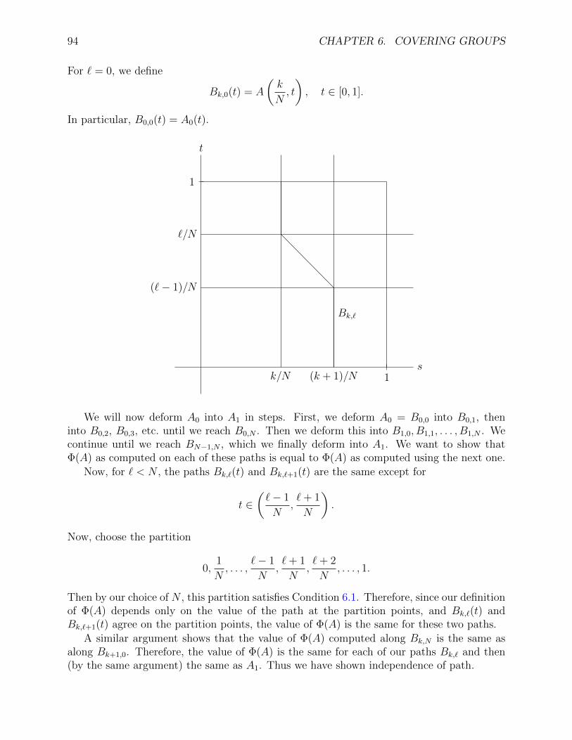
94 CHAPTER 6. COVERING GROUPS
For ` = 0, we define
Bk,0(t) = A
(k
N, t
), t ∈ [0, 1].
In particular, B0,0(t) = A0(t).
s
t
k/N (k + 1)/N 1
(`− 1)/N
`/N
1
Bk,`
We will now deform A0 into A1 in steps. First, we deform A0 = B0,0 into B0,1, theninto B0,2, B0,3, etc. until we reach B0,N . Then we deform this into B1,0, B1,1, . . . , B1,N . Wecontinue until we reach BN−1,N , which we finally deform into A1. We want to show thatΦ(A) as computed on each of these paths is equal to Φ(A) as computed using the next one.
Now, for ` < N , the paths Bk,`(t) and Bk,`+1(t) are the same except for
t ∈(`− 1
N,`+ 1
N
).
Now, choose the partition
0,1
N, . . . ,
`− 1
N,`+ 1
N,`+ 2
N, . . . , 1.
Then by our choice of N , this partition satisfies Condition 6.1. Therefore, since our definitionof Φ(A) depends only on the value of the path at the partition points, and Bk,`(t) andBk,`+1(t) agree on the partition points, the value of Φ(A) is the same for these two paths.
A similar argument shows that the value of Φ(A) computed along Bk,N is the same asalong Bk+1,0. Therefore, the value of Φ(A) is the same for each of our paths Bk,` and then(by the same argument) the same as A1. Thus we have shown independence of path.
6.6. COVERING GROUPS 95
Step 5. One can show that Φ is a homomorphism as follows. For A,B ∈ G, choose pathA(t) and B(t) from I to A and B, respectively. Then construct a path C(t) from I to ABby
C(t) =
{C(t) = A(2t) t ∈ [0, 1/2],
C(t) = AB(2t− 1) t ∈ [1/2, 1].
Then it follows from the definition of Φ above that Φ(AB) = Φ(A)Φ(B) (see Exercise 6.5.1).Now, since Φ is defined near the identity as Φ = exp ◦φ ◦ log, we have
d
dtΦ(etX)∣∣t=0
=d
dtetφ(X)
∣∣t=0
= φ(X).
Therefore φ is the Lie algebra homomorphism associated to the Lie group homomorphismΦ, as desired.
Exercises.
6.5.1. Complete Step 5 of the proof of Theorem 6.5.1 by showing that Φ(AB) = Φ(A)Φ(B).
6.6 Covering groups
Definition 6.6.1 (Universal covering group). Suppose G is a connected Lie group. Thena universal covering group (or universal cover) of G is a simply connected Lie group Gtogether with a Lie group homomorphism Φ: G → G such that the associated Lie algebrahomomorphism φ : g→ g is a Lie algebra isomorphism. The homomorphism Φ is called thecovering homomorphism (or projection map).
Note that this theorem does not specify that the Lie groups be matrix Lie groups. Infact, the universal cover of matrix Lie group may be a nonmatrix Lie group. For instance, the
universal covering group ˜SL(2,C) of SL(2,C) is a nonmatrix Lie group. However, universalcovering groups always exist, as the next theorem tells us.
Theorem 6.6.2 (Existence and uniqueness of universal covering groups). For any connectedLie group, a universal cover exists. If G is a connected Lie group and (H1,Φ1) and (H2,Φ2)are universal covers of G, then there exists a Lie group isomorphism Ψ: H1 → H2 such thatΦ2 ◦Ψ = Φ1. In other words, the diagram
H1
Φ1
Ψ // H2
Φ2~~G
commutes.
96 CHAPTER 6. COVERING GROUPS
Proof. We will not prove the existence part of this theorem (see [Hal03, App. C]). Uniquenessfollows from Theorem 6.5.1 as follows. Suppose (H1,Φ1) and (H2,Φ2) are universal coversof G. Then the corresponding Lie algebra maps φ1, φ2 are isomorphisms. By Theorem 6.5.1,there exists a Lie group homomorphism Ψ: H1 → H2 corresponding to the isomorphismφ−1
2 ◦ φ1 : h1 → h2 of their Lie algebras and a Lie group homomorphism Ψ′ : H2 → H1
corresponding to φ−11 ◦ φ2. Then, the composition Ψ′ ◦ Ψ: H1 → H1 corresponds to the
identity Lie algebra homomorphism. By the uniqueness statement in Theorem 6.5.1, wehave Ψ′ ◦ Ψ = idH1 . Similarly, Ψ ◦ Ψ′ = idH2 . Again, by the uniqueness statement inTheorem 6.5.1, we have Φ2 ◦Ψ = Φ1.
Remark 6.6.3. (a) Since the universal cover of a Lie group G is unique up to isomorphism,we often speak of the universal cover.
(b) If G is a simply connected Lie group and φ : g → g is a Lie algebra isomorphism, thenby Theorem 6.5.1, there exists a Lie group homomorphism Φ: G→ G inducing φ. Thisyields a universal cover of G. Using φ, we can identify g and g. Thus, by a slight abuseof terminology, we sometimes think of the universal cover of G as the unique simplyconnected Lie group with the same Lie algebra as G (we use the identity map g→ g toconstruct the covering homomorphism).
(c) A covering group (not necessarily universal) of a connected Lie group G is a connectedLie group H (not necessarily simply connected) together with a Lie group homomor-phism Φ: H → G such that the associated Lie algebra homomorphism φ : h → g is anisomorphism. In general, a Lie group can have many nonisomorphic covering groups,with different fundamental groups.
Examples 6.6.4. (a) G = S1. The universal cover is R and the covering homomorphism isthe map R→ S1 given by θ 7→ eiθ.
(b) G = SO(3). The universal cover is SU(2) and we have described the covering homomor-phism in Section 1.5.
(c) G = U(n). The universal cover is R × SU(n) and the covering homomorphism is themap
R× SU(n)→ U(n), (θ, U) 7→ eiθU. (6.3)
Since R and SU(n) are simply connected, R×SU(n) is simply connected. The Lie algebrahomomorphism associated to (6.3) is
R⊕ su(n) 7→ u(n), (r, A) 7→ irI + A, r ∈ R, A ∈ su(n). (6.4)
It thus suffices to check that (6.4) is a Lie algebra isomorphism and that (6.3) is a Liegroup homomorphism (Exercise 6.6.1).
(d) As discussed before, the universal cover of SO(n), n ≥ 3, is Spin(n) and these are doublecovers (i.e. the covering homomorphisms are 2-to-1).
6.7. SUBGROUPS AND SUBALGEBRAS 97
Remark 6.6.5. In the above examples, the universal covers are all matrix Lie groups. Ingeneral, one can show that the universal cover of a compact matrix Lie group is again amatrix Lie group (not necessarily compact).
Remark 6.6.6. The universal covering construction is inverse to the process of taking thequotient by a discrete subgroup because the kernel of the covering homomorphism G → Gis a discrete subgroup of G, called the fundamental group of G. It can be shown that thefundamental group of a Lie group is always abelian, even though the fundamental group of anarbitrary smooth manifold can be any finitely presented group (finite number of generatorsand relations). Thus, the topology of Lie groups is rather constrained.
Remark 6.6.7. If a simply connected Lie group with Lie algebra g has a discrete centre, thenthe set of all connected Lie groups with Lie algebra g form a lattice, corresponding to thelattice of subgroups of the centre of the simply connected Lie group. For example, thishappens with g = sl(2, F ), where F = R or C. The Lie group SL(2, F ) has universal cover˜SL(2, F ) and every Lie group with Lie algebra g has ˜SL(2, F ) as its universal cover and is a
cover of PSL(2, F ) := SL(2, F )/Z(SL(2, F )), where Z(SL(2, F )) = {±1}.
Exercises.
6.6.1. Prove the following:
(a) The map (6.4) is a Lie algebra isomorphism.
(b) The map (6.4) is the Lie algebra homomorphism corresponding to the map (6.3).
(c) The map (6.3) is a Lie group homomorphism.
6.7 Subgroups and subalgebras
Given the close connections between Lie groups and Lie algebras, it seems natural to expectthat there is a relationship between the subgroups of a Lie group and the subalgebras of itsLie algebra. If G and H are matrix Lie groups with H ⊆ G, then it is clear that h is a Liesubalgebra of g. In general the converse is false, as the following example illustrates.
Example 6.7.1. Consider the matrix Lie group GL(2,C), with Lie algebra gl(2,C). If we fixan irrational number a, then
h =
{(it 00 ita
) ∣∣∣∣ t ∈ R}
(6.5)
98 CHAPTER 6. COVERING GROUPS
is a one-dimensional real subalgebra of gl(2,C). Any matrix Lie group H with Lie algebrah would have to contain
H0 = exp(h) =
{(eit 00 eita
) ∣∣∣∣ t ∈ R}.
Being a matrix Lie group, H would need to be closed in GL(2,C). But the closure of H0 inGL(2,C) is
H1 =
{(eit 00 eis
) ∣∣∣∣ s, t ∈ R}.
Then h would have to contain the Lie algebra of H1, which is two dimensional. This is acontradiction. Thus, there is no matrix Lie group corresponding to h.
The problem in Example 6.7.1 is due to the fact that we are restricting our attention tomatrix Lie groups. We can resolve the issue by relaxing this condition.
Definition 6.7.2 (Lie algebra of an arbitrary matrix group). Suppose H is any subgroupof GL(n,C). We define the Lie algebra of H to be the set
{X ∈Mn(C) | etX ∈ H for all t ∈ R}. (6.6)
Definition 6.7.3 (Connected Lie subgroup). Suppose G is a matrix Lie group with Liealgebra g. We say H ⊆ G is a connected Lie subgroup (or analytic subgroup) of G if thefollowing conditions are satisfied:
(a) H is a subgroup of G.
(b) The Lie algebra h of H is a subspace of g.
(c) Every element of H can be written in the form eX1eX2 · · · eXm , with X1, . . . , Xm ∈ h.
Example 6.7.4. The group H0 of Example 6.7.1 is a connected Lie subgroup of GL(2,C) withLie algebra h given by (6.5).
The word connected in Definition 6.7.3 is justified by the following result.
Proposition 6.7.5. If H is a connected Lie subgroup of a matrix Lie group G, then H ispath-connected.
Proof. It suffices to show that any element of H can be connected to the identity by acontinuous path taking values in H. We will prove, by induction on m, that any element ofH of the form
h = eX1eX2 · · · eXm , m ∈ N, X1, . . . , Xm ∈ h,
can be connected to the identity by a continuous path lying in H. Since H is a connectedLie subgroup of G, all elements of H are of this form.
For m = 0, we have h = 1 and the result is trivial. Assume m ≥ 1 and that the result istrue for m− 1. For X1, . . . , Xm ∈ h, define the continuous path
h(t) = eX1eX2 · · · eXme−tXm = eX1eX2 · · · e(1−t)Xm .
6.7. SUBGROUPS AND SUBALGEBRAS 99
By the definition of h, we have e−tXm ∈ H for all t ∈ R. Thus h(t) is contained in H. Wehave h(0) = eX1eX2 · · · eXm and h(1) = eX1eX2 · · · eXm−1 . By the induction hypothesis, thereis a path, contained in H, connecting h(1) to the identity. This completes the proof of theinductive step.
Proposition 6.7.6. Suppose H is a connected Lie subgroup of a matrix Lie group G. Thenthe Lie algebra h of H is a subalgebra of the Lie algebra g of G.
Proof. If A ∈ H and Y ∈ h, then, for all t ∈ R, we have
etAY A−1
= AetYA−1 ∈ H.
Thus AY A−1 ∈ h. It follows that, for X, Y ∈ h,
etXY e−tX ∈ h for all t ∈ R.
Since h is a vector space, it is a topologically closed subset of Mn(C). Therefore, for X, Y ∈ h,
[X, Y ] = XY − Y X =d
dtetXY e−tX
∣∣∣∣t=0
= limh→0
ehXY e−hX − Yh
∈ h.
Therefore h is a Lie subalgebra of g.
Theorem 6.7.7. Suppose G is a matrix Lie group with Lie algebra g, and let h be a Liesubalgebra of g. Then
H = {eX1eX2 · · · eXm | X1, . . . , Xm ∈ h}
is the unique connected Lie subgroup H of G such that the Lie algebra of H is h.
We will not prove Theorem 6.7.7. A proof can be found in [Hal03, §3.8]. The connectedLie subgroup H corresponding to the subalgebra h in Theorem 6.7.7 may or may not bematrix Lie group. It is a matrix Lie group precisely when H is a closed subset of G.However, we have the following result.
Theorem 6.7.8. Suppose that G is a matrix Lie group and that H is a connected Liesubgroup of G. Then H can be given the structure of a Lie group in such a way that theinclusion of H into G is a Lie group homomorphism.
Proof. We give only a sketch of the proof. We first note that the topology on H induced fromthe topology on G can be very bad. For example, H might not even be locally connected inthis topology. So, in general, we need a different topology on H. For any A ∈ H and ε > 0,define
UA,ε = {AeX | X ∈ h, ‖X‖ < ε}.
We then define a topology on H by using the UA,ε as basic open sets. More precisely, wedefine a subset U ⊆ H to be open if, for all A ∈ U , there exists ε > 0 such that UA,ε ⊆ U .
In fact, H can be made into a smooth manifold by using the sets UA,ε as basic coordinateneighbourhoods, and using the maps X 7→ AeX as local coordinate maps. One can then show
100 CHAPTER 6. COVERING GROUPS
that the product and inverse maps on H are smooth with respect to this smooth manifoldstructure.
Finally, one can show that any set of H that is open in the topology induced from thetopology of G is also open in the topology defined above. It follows that the inclusion of Ginto H is continuous (the preimage of open sets are open).
Theorem 6.7.9. Every finite-dimensional real Lie algebra is isomorphic to the Lie algebraof some Lie group.
Proof. We give only a sketch of the proof. Ado’s Theorem (which we have not proven)states that every finite-dimensional real Lie algebra is isomorphic to a subalgebra of gl(n,R).Theorem 6.7.8 then implies that there is a Lie group with this Lie algebra. We are implicitlyusing here the fact that the more abstract definition of the Lie algebra of a (general) Liegroup coincides with Definition 6.7.2 for connected Lie subgroups.
Proposition 6.7.10. The association of the Lie algebra to a Lie group yields a one-to-one correspondence between isomorphism classes of simply connected (real) Lie groups andisomorphism classes of finite-dimensional real Lie algebras.
Proof. Let F be the map from the set of isomorphism classes of simply connected Lie groupsto the set of isomorphism classes of real Lie algebras given by taking the Lie algebra of aLie group. Then F is injective by Corollary 6.5.2. Suppose g is a real Lie algebra. Then, byTheorem 6.7.9, there exists a Lie group G with Lie algebra g. By Theorem 6.6.2, G has auniversal cover G with Lie algebra g. Thus F is surjective.
Another way of summarizing some of the results above is that when we restrict the functorfrom Lie groups to Lie algebras given in Theorem 5.13.1 to the (full) subcategory of simplyconnected Lie groups, it yields an equivalence of categories between the category of simplyconnected Lie groups and the category of finite-dimensional real Lie algebras.
Chapter 7
Further directions of study
In this course, we have only scratched the surface of the topic of Lie groups. There is muchmore to learn. In this final chapter we give a brief (and not, by any means, comprehensive)overview of some further directions of study.
7.1 Lie groups, Lie algebras, and quantum groups
One obvious direction of further study is to expand one’s focus to all Lie groups, instead ofjust matrix Lie groups. As we saw in Chapter 6, this more general viewpoint is necessaryif one wants to fully discuss topics just as covering groups, quotients by normal subgroups(for example, there is a quotient of the Heisenberg group that is not a matrix Lie group—see[Sti08, p. 72]), etc.
The study of Lie algebras themselves is also a very active area of research. The finite-dimensional simple complex Lie algebras have been classified. A more general class of Liealgebras are the so-called Kac–Moody algebras . The affine Lie algebras can, in some sense,be viewed as the next step beyond finite-dimensional simple Lie algebras. They play animportant role in physics and the theory of vertex algebras. The books [EW06, Hum78] aregood references for the finite-dimensional theory, while [Kac90] is a standard reference forthe infinite-dimensional setting.
To any Lie algebra, one can associated its universal enveloping algebra. It is an associativealgebra that has the same representation theory as the original Lie algebra. These universalenveloping algebras can be q-deformed to produce quantum groups or quantized envelopingalgebras . Taking the parameter q to 1 recovers the original enveloping algebra. On the otherhand, taking q to zero results in a structure known as a crystal , where algebra is replaced bycombinatorics. This construction plays a central role in combinatorial representation theory.The books [HK02, Kas95] are good references for these topics.
7.2 Superalgebras and supergroups
An interesting and active area of research is the generalization from the “standard” setting tothe “super” setting. A supermanifold is similar to a manifold, except that instead of lookinglocally like Rn for some n, it looks like the superspace Rm|n. The variables corresponding to
101
102 CHAPTER 7. FURTHER DIRECTIONS OF STUDY
the n “odd” coordinates supercommute (xy = −yx) instead of commute. A Lie supergroupis then a group object in the category of supermanifolds (see Definition 1.1.4).
The tangent space of a Lie supergroup is naturally a Lie superalgebra. A Lie superalgebrais a Z2-graded vector space g = g0 + g1 with a bilinear operation [·, ·] : g× g→ g (the superLie bracket) satisfying the following conditions:
(a) It respects the grading: [gi, gj] ⊆ gi+j for i, j ∈ Z2,
(b) It is super skew-symmetric: [x, y] = −(−1)|x||y|[y, x] for all homogeneous x, y ∈ g (here|x| denotes the parity of x, i.e. x ∈ g|x|).
(c) It satisfies the super Jacobi identity:
[x, [y, z]] = [[x, y], z] + (−1)|x||y|[y, [x, z]] for all homogeneous x, y, z ∈ g.
A Lie superalgebra g with g1 = 0 is simply a Lie algebra. The study of Lie superalgebrasand Lie supergroups plays an important role in supersymmetry in physics. Many results inLie algebras have been generalized to Lie superalgebras (for instance, the classification ofthe complex simple Lie superalgebras). However, there are also many examples of theoremsknown in the Lie algebra case that have not yet been extended to the Lie superalgebra case.
7.3 Algebraic groups and group schemes
Moving from the setting of smooth manifolds to the setting of algebraic geometry resultsin a passage from Lie groups to algebraic groups. More precisely, an algebraic group is agroup object in the category of algebraic varieties (see Section 1.1). Explicitly, an algebraicgroup (or group variety) is a group that is an algebraic variety, such that the multiplicationand inversion operations are given by regular functions on the variety. Over a field, affinealgebraic groups (where the algebraic variety is an affine variety) are matrix groups. Thus,over the real numbers, the definition of an algebraic group is more restrictive than thedefinition of a Lie group.
Schemes are generalizations of algebraic varieties. A group object in the category ofschemes is called a group scheme. There is a well-developed theory of group schemes andthis topic continues to be an active area of research.
7.4 Finite simple groups
Killing and Cartan classified the simple Lie groups. This helped pave the way for a classi-fication of the finite simple groups. Each matrix Lie group G gives rise to infinitely manyfinite groups by replacing the entries of G by elements of a finite field (say, the integersmodulo some prime p). Since there is a finite field of size q for each prime power q, there areinfinitely many finite groups corresponding to each infinite matrix Lie group. In fact, eachsimple Lie group yields infinitely many finite simple groups in this way. These are called thesimple finite groups of Lie type.
7.5. REPRESENTATION THEORY 103
Theorem 7.4.1 (Classification of finite simple groups). Every finite simple group is
• a cyclic group of prime order,
• an alternating group of degree at least 5,
• a simple group of Lie type, or
• one of 26 sporadic groups.
The largest sporadic group is called the Monster group.
7.5 Representation theory
Once one has learned about the structure of Lie groups themselves, it is natural to investigatetheir representations. A (real) representation of a Lie group G is a Lie group homomorphism
G→ GL(n,R) or G→ GL(V ),
where V is a real vector space. Complex representations are defined similarly.Representations can be thought of as an action of a group on a vector space. The term
“representation” comes from this interpretation—each element of G is “represented” as alinear map on a vector space.
We now know that each complex representation of complex Lie group G yields a Liealgebra homomorphism
g→ gl(n,C) or g→ gl(V ),
called a representation of g. Often one can answer questions about representations of Liegroups by studying representations of the corresponding Lie algebra, which are often mucheasier to study. The later chapters of [Hal03] concern the representation theory of Lie groups.
The study of representations of finite groups (e.g. permutation groups) is also an impor-tant and interesting topic and does not require knowledge of Lie groups or Lie algebras.
Index
3-sphere of unit quaternions, 8
absolute valueof a matrix, 52
absolute value of quaternions, 7adjoint mapping, 76affine Lie algebra, 101algebraic group, 102alternating, 51analytic subgroup, 98
C∗, 26Campbell–Baker–Hausdorff Theorem, 81Cartan–Dieudonne Theorem, 14category, 1centres, 44circle group, 3circle Lie group, 4classical groups, 44classical Lie groups, 20Clifford algebra, 91compact, 36compact classical groups, 44compact symplectic group, 24complex general linear group, 21complex matrix Lie group, 61complex orthogonal group, 23complex special linear group, 21complex symplectic group, 24complexification
of a Lie algebra, 62of a vector space, 61
component, 29composition, 1conjugation, 10connected component, 29connected Lie subgroup, 98convergence of matrices, 20
covering group, 96covering homomorphism, 95covering space, 87crystal, 101
δ-neighbourhood, 69derivative of a path, 56differentiable path, 55Dirac’s belt trick, 14direct product, 17discrete subgroup, 46distance between matrices, 46dot product, 21double cover, 14, 91
E(n), 26Euclidean group, 26Euclidean space, 3exponential map
to SO(2), 47to SU(2), 48
exponential of a matrix, 53
finite group, 21finite simple groups, 102functor, 73fundamental group, 97
gauge group, 3general linear group, 3GL(n,C), 21gl(n,C), 60GL(n,R), 21gl(n,R), 60group, 2
circle, 3linear, 3simple, 14
group action, 103
104
INDEX 105
group object, 2group scheme, 102group variety, 102groups of Lie type, 102
Heisenberg group, 3, 25homeomorphism, 70homomorphism of Lie groups, 27hyperplane, 14
ideal of a Lie algebra, 51inner product on Rn, 21inverse, 2isometry, 14isomorphism of Lie groups, 27
J , 24J2n, 25Jacobi identity, 51
Kac–Moody algebra, 101
Lie algebra, 51alternate description, 70of a Lie group, 60of arbitrary matrix group, 98
Lie bracket, 50, 51Lie group, 3, 37Lie group homomorphism, 27Lie group isomorphism, 27lie over, 86Lie polynomial, 81Lie product formula, 71Lie superalgebra, 102Lie supergroup, 102lift, 87linear group, 3, 4, 20linear Lie group, 20local homeomorphism, 87log, 64logarithm, 64Lorentz group, 3
matrix absolute value, 52matrix exponential, 53matrix group, 4, 20matrix Lie group, 3, 20
complex, 61matrix logarithm, 64maximal torus, 39metaplectic group, 25Monster group, 103morphism, 1Mp(n,R), 25
neighbourhood, 69nilpotent matrix, 55normal subgroup, 14, 45, 78normal subgroups
of SO(n), SU(n), Sp(n), 79
object, 1group, 2terminal, 1
O(n), 12, 22, 26o(n), 60O(n,C), 23o(n,C), 60one-parameter subgroup, 72orientation-preserving, 15orientation-reversing, 15orthogonal group, 3, 12, 22, 26
path, 29derivative, 56differentiable, 55smooth, 55
path-connected, 29Poincare group, 3polar decomposition, 33
SL(n,C), 35SL(n,R), 34
positive definite, 34, 35positive matrix, 34, 35positive semidefinite, 35projection map, 95pure imaginary quaternions, 9
quantized enveloping algebra, 101quantum group, 101quaternion conjugate, 8quaternions, 6
3-sphere, 8
106 INDEX
absolute value, 7pure imaginary, 9
R∗, 26real form, 64real general linear group, 21real special linear group, 21real symplectic group, 24reflection in a hyperplane, 14representation, 103Rn, 26rotation, 15
S1, 4, 26scheme, 102Schreier’s Theorem, 46sequential tangent vector, 67simple group, 14, 45simple groups, 102simple Lie algebra, 51simplicity of SO(2m+ 1), 79simplicity of so(n), su(n), sp(n), 79simply connected, 85skew-Hermitian, 57skew-symmetric, 57SL(n,C), 21slnCsl(n,C), 60SL(n,R), 21sl(n,R), 60smooth path, 55SO(2), 4SO(n), 12, 22so(n), 60SO(n,C), 23so(n,C), 60special complex orthogonal group, 23special linear group, 3special orthogonal group, 4, 12, 22special unitary group, 8, 22spin groups, 91Sp(n), 24sp(n), 60Sp(n,C), 24sp(n,C), 60Sp(n,R), 24
sp(n,R), 60sporadic group, 103su(2), 51subgroup
discrete, 46normal, 14, 45, 78
submultiplicative property, 52SU(n), 8, 22su(n), 60supermanifold, 101symmetric matrix, 33symplectic group, 24
complex, 24real, 24
tangentsequential, 67
tangent space, 56of SU(2), 49
tangent space visibility, 78tangent vector, 56terminal object, 1topological dimension, 70torus, 39translation, 26
U(n), 8, 22u(n), 60unitary group, 3, 8, 22universal cover, 95universal covering group, 95universal enveloping algebra, 101
Bibliography
[EW06] Karin Erdmann and Mark J. Wildon. Introduction to Lie algebras. Springer Un-dergraduate Mathematics Series. Springer-Verlag London, Ltd., London, 2006.
[Hal03] Brian C. Hall. Lie groups, Lie algebras, and representations, volume 222 of Grad-uate Texts in Mathematics. Springer-Verlag, New York, 2003. An elementaryintroduction.
[HK02] Jin Hong and Seok-Jin Kang. Introduction to quantum groups and crystal bases,volume 42 of Graduate Studies in Mathematics. American Mathematical Society,Providence, RI, 2002.
[Hum78] James E. Humphreys. Introduction to Lie algebras and representation theory, vol-ume 9 of Graduate Texts in Mathematics. Springer-Verlag, New York-Berlin, 1978.Second printing, revised.
[Kac90] Victor G. Kac. Infinite-dimensional Lie algebras. Cambridge University Press,Cambridge, third edition, 1990.
[Kas95] Christian Kassel. Quantum groups, volume 155 of Graduate Texts in Mathematics.Springer-Verlag, New York, 1995.
[Sti08] John Stillwell. Naive Lie theory. Undergraduate Texts in Mathematics. Springer,New York, 2008.
107