Introduction to Macro Data

Karel Mertens, Cornell University

Contents

1 US Data 3

2 Detrending and filtering 8

2.1 The Growth Rate . . . . . . . . . . . . . . . . . . . . . . . . . . . . . . . . . 8

2.2 Deterministic Detrending . . . . . . . . . . . . . . . . . . . . . . . . . . . . 9

2.3 Hodrick-Prescott filter . . . . . . . . . . . . . . . . . . . . . . . . . . . . . . 10

2.4 Other Methods . . . . . . . . . . . . . . . . . . . . . . . . . . . . . . . . . . 11

3 Stylized Facts 12

1

References

Backus, D. and Kehoe, P. (1982), ‘International evidence on the historical properties of

business cycles’, American Economic Review 82(4).

Beveridge, S. and Nelson, C. (1981), ‘A new approach to the decomposition of economic

time series into permanent and transitory components with particular attention to the

measurement of the business cycle’, Journal of Monetary Economics 7(2).

Canova, F. (2007), Methods for Applied Macroeconomic Research, Princeton University

Press.

Christiano, L. and Fitzgerald, T. (2003), ‘The band pass filter’, International Economic

Review 44(2).

Francis, N. and Ramey, V. (2009), ‘Measures of per capita hours and their implications for

the technology-hours debate’, Journal of Money, Credit and Banking 41(6).

Hamilton, J. (1989), ‘A new approach to the economic analysis of nonstationary time series

aand the business cycle.’, Econometrica 57(2).

King, R. G. and Rebelo, S. T. (1999), ‘Resuscitating real business cycles’, Handbook of

Macroeconomics 1.

Ravn, M. and Uhlig, H. (2002), ‘On adjusting the hodrick-prescott filter for the frequency

of observations’, The Review of Economics and Statistics 84(2).

Stock, J. H. and Watson, M. W. (1999), ‘Business cycle fluctuations in us macroeconomic

time series’, Handbook of Macroeconomics 1.

Whelan, K. (2002), ‘A guide to us chain-weighted data.’, Review of Income and Wealth

48(2).

2

Figure 1: Real Per Capita Expenditures

1950 1960 1970 1980 1990 2000 2010−2

−1.5

−1

−0.5

0

0.5

1

1.5

2

2.5

3

Log

Leve

ls

real gdpreal nondur cons expreal dur cons expreal fix inv expreal gov exp

1 US Data

Figure 1 plots time series for per capita (adult) real output, per capita real consumption, per

capita investment and per capita hours worked for the US over the sample 1948Q1:2012Q4.1

Note that there is trend growth in output, consumption and investment. At shorter fre-

quencies the output series display recurrent and large fluctuations about its trend known as

business cycles. Moreover, the other time series seem to comove with the output series. The

objective of many macro models is to generate endogenous dynamic behavior conditional

on exogenous factors that resemble the behavior of the empirical time series, either at long

run frequencies, short run frequencies or both.

Because many macroeconomic time series display trend growth, it is not immediately ob-

vious what the cyclical properties of the data are. Many business cycle models generate

cyclical variability in response to transitory exogenous events. To make a comparison of the

model dynamics with the cyclical properties of the empirical data, we need a procedure, a

detrending method, to extract the cyclical component of the actual time series. However,

1You can download an excel file with the data on the course website.

3

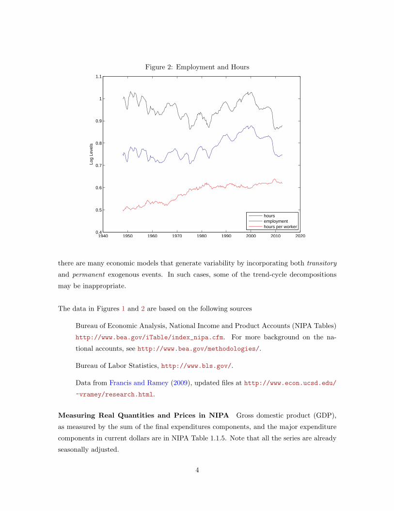
Figure 2: Employment and Hours

1940 1950 1960 1970 1980 1990 2000 2010 20200.4

0.5

0.6

0.7

0.8

0.9

1

1.1

Log

Leve

ls

hoursemploymenthours per worker

there are many economic models that generate variability by incorporating both transitory

and permanent exogenous events. In such cases, some of the trend-cycle decompositions

may be inappropriate.

The data in Figures 1 and 2 are based on the following sources

Bureau of Economic Analysis, National Income and Product Accounts (NIPA Tables)

http://www.bea.gov/iTable/index_nipa.cfm. For more background on the na-

tional accounts, see http://www.bea.gov/methodologies/.

Bureau of Labor Statistics, http://www.bls.gov/.

Data from Francis and Ramey (2009), updated files at http://www.econ.ucsd.edu/

~vramey/research.html.

Measuring Real Quantities and Prices in NIPA Gross domestic product (GDP),

as measured by the sum of the final expenditures components, and the major expenditure

components in current dollars are in NIPA Table 1.1.5. Note that all the series are already

seasonally adjusted.

4

Table 1: Current Dollars (NIPA Table 1.1.5)

Line More detail1 Gross domestic product 2 + 7 + 15 +222 Personal consumption expenditures 3+4 NIPA Table 2.3.53 Goods 4+54 Durable goods5 Nondurable goods6 Services

7 Gross private domestic investment 8+148 Fixed investment 9 +13 NIPA Table 5.3.59 Nonresidential 10+11+1210 Structures11 Equipment12 Intellectual property products13 Residential14 Change in private inventories

15 Net exports of goods and services 16-19 NIPA Table 4.2.516 Exports 17+1817 Goods18 Services19 Imports 20+2120 Goods21 Services

22 Government consumption exp. and gross inv. 23+26 NIPA Table 3.9.523 Federal 24+2524 National defense25 Nondefense26 State and local

Aggregate real quantity indices qindext are computed using prices Pt(i) and current dollar

amounts Pt(i)qt(i) as chained indices based on the Fisher index formula,

qindext = qindext−1

√( ∑ni=1 Pt(i)qt(i)∑n

i=1 Pt(i)qt−1(i)

)( ∑ni=1 Pt−1(i)qt(i)∑n

i=1 Pt−1(i)qt−1(i)

)(Table 1.1.3)

with the value for some base period fixed to 100. Currently the base year is 2009. Chained

price indices P indext are computed as

P indext = P index

t−1

√( ∑ni=1 Pt(i)qt(i)∑n

i=1 Pt−1(i)qt(i)

)( ∑ni=1 Pt(i)qt−1(i)∑n

i=1 Pt−1(i)qt−1(i)

)(Table 1.1.4)

5

with the value for some base period fixed to 100. The quantity indices for GDP and the

main expenditure components are in NIPA Table 1.1.3 and the price indices are in NIPA

Table 1.1.4.

Current-dollar (nominal) aggregates for GDP and the main expenditure components are,

Qcurrent$t =

n∑i=1

Pt(i)qt(i) (NIPA Table 1.1.5)

The chained-dollar value qchain$t is calculated by multiplying the quantity index by the

base-period current-dollar value and dividing by 100, i.e.

qchain$t = qindext ×Qcurrent$2009 /100 (NIPA Table 1.1.6)

Finally, the implicit price deflators are alternative measures of aggregate nominal price

levels. These deflators are defined as as the ratio of the current-dollar value to the corre-

sponding chained-dollar value times 100:

P IPDt = Qcurrent$

t /qchain$t × 100 (NIPA Table 1.1.9)

The implicit price deflators P IPDt and the price indices P index

t are typically very similar.

Obtaining measures of real quantities that are comparable to model generated data of-

ten requires summing or subtracting different expenditure components. For instance, the

measure of nondurable consumption in Figure 1 is based on the sum of expenditures on

nondurable goods and services. Unlike the current dollar values, adding up chained real

measures can be misleading when there are important relative price changes, see Whelan

(2002). In principle, a new measure must be computed by re-aggregating over all sub-

components according to the formulas above. Unfortunately, most researchers do not have

access the detailed data underlying the aggregates. However, a good approximation can

usually be found by chain-adding the aggregate data. For instance, suppose we want a real

measure of the sum of components X and Y, i.e. qX+Yt , based on current value data from

Table 1.1.5 and price indices PXt and P Y

t from Table 1.1.4. Rather than approximating by

6

qXt + qYt , a better procedure is chain-adding:

qX+Yt = qXt

chain+ qYt = qX+Y

t−1

√√√√( PXt qXt + P Y

t qYtPXt qXt−1 + P Y

t qYt−1

)(PXt−1q

Xt + P Y

t−1qYt

PXt−1q

Xt−1 + P Y

t−1qYt−1

)(Chain-Adding)

with the value for some base period fixed to 100.

Population and Labor Supply Data on population, hours worked and employment

is available from the Bureau of Labor Statistics. More comprehensive measures that also

include the government sector require additional data that is not readily available from the

BLS website, but can be found in appendix to Francis and Ramey (2009). Total Popu-

lation is the sum of the total civilian noninstitutional population age 16 and over (BLS

series ID LNS10000000, quarterly average of monthly data) and total employed in the armed

forces from Francis and Ramey (2009). Total hours and total employment are also from

Francis and Ramey (2009).

The series in Figure 1 are the log of ratios of quantity indices divided by total popula-

tion. Hours and employment in Figure 2 are also in logs after dividing by total population.

Hours per worker is the log of the hours-employment ratio.

7

2 Detrending and filtering

Time series such as real output yt (real GDP per capita) can be thought of as consisting of

a cyclical component yct and a trend component yxt , i.e.

yt = yxt + yct

There are numerous ways to separate yct from yxt .2 The terms detrending and filtering are

often used interchangeably to describe this separation, but are distinct procedures. Detrend-

ing is the process of making economic series (covariance) stationary, which is necessary for

instance to compute second moments. Filtering is a much broader concept. A filter is an

operator that removes movements at particular frequencies. Business cycles have frequen-

cies corresponding to cycles of 6 to 32 quarters, which is in the range of the business cycle

periodicity reported by the NBER and CEPR. A filter that extracts movements at these

frequencies therefore extracts the cyclical movements of interest.

2.1 The Growth Rate

It is possible to assume that the growth rate of yt captures the cyclical component:

yct = ∆yt yxt = yt−1

Figures 1 and 2 show annualized quarterly growth as well as year-over-year growth in real

GDP per capita. The shaded areas denote NBER-dated recessions.3

2See Canova (2007, Ch. 3) for an overview.3NBER Business Cycle Dates are available at http://www.nber.org/cycles.html

8

Figure 3: Growth US Real GDP per capita

1950 1960 1970 1980 1990 2000 2010

−0.1

−0.05

0

0.05

0.1

0.15

Ann

ualiz

ed Q

uart

erly

Gro

wth

1950 1960 1970 1980 1990 2000 2010−0.04

−0.02

0

0.02

0.04

0.06

0.08

0.1

Yea

r−ov

er−

Yea

r G

row

th

2.2 Deterministic Detrending

A trend of a time series can be taken to be deterministic and the cyclical component is then

measured as the residual of a regression of yt on polynomials in time.

yt = a0 +J∑

j=1

ajtj + yct , Corr(yxt , y

ct ) = 0

The a’s and the residual yct can be easily estimated by OLS. Figure 4 shows the case of a

simple linear trend J = 1.

9

Figure 4: US Real GDP per capita: linear deterministic trend

1940 1950 1960 1970 1980 1990 2000 2010 2020−9

−8.5

−8

−7.5

Logl

evel

1950 1960 1970 1980 1990 2000 2010

−0.1

−0.05

0

0.05

Cyc

lical

com

pone

nt

2.3 Hodrick-Prescott filter

The Hodrick-Prescott (HP) filter is one of the most popular methods to extract cyclical

components. First, trend and cycle are assumed to be uncorrelated. Second, the trend is a

smooth process, which is made operational by penalizing variations in the second difference

of the trend:

minyxt

{T∑t=0

(yt − yxt )2 + λ

T−1∑t=2

((yxt+1 − yxt )− (yxt − yxt−1)

)2}

As λ increases the trend becomes smoother and for λ → ∞ it becomes linear. The literature

typically selects the value of λ a priori to carve out particular frequencies. For quarterly

US data, λ = 1600 is typically chosen, which implies that cycles longer than six to seven

years are attributed to the trend. Note that for other data frequencies and sometimes also

for other countries, the value of λ has to be adjusted, see Ravn and Uhlig (2002).

10

Figure 5: US Real GDP per capita: HP filter

1940 1950 1960 1970 1980 1990 2000 2010 2020−9

−8.5

−8

−7.5

Logl

evel

1950 1960 1970 1980 1990 2000 2010

−0.04

−0.02

0

0.02

Cyc

lical

com

pone

nt

2.4 Other Methods

The Beveridge and Nelson (1981) decomposition assumes a stochastic trend and that the

long-run forecast is a measure of the trend. If yt is stationary in first differences, the BN

decomposition yields a trend that follows a unit root and a stationary cyclical component.

The regime shifting decomposition of Hamilton (1989) assumes that the trend is regime

specific, that the trend is deterministic within a regime, but that regime itself is stochas-

tically varying over time. The exponential smoothing filter is very similar to the HP filter,

but penalizes the changes in the trend instead of the acceleration of the trend. Moving

average filters are based on average of a specified number of leads and/or lags. Most of

these filters remove the low frequencies, but leave the high frequencies (they are high pass

filters). Band pass filters eliminate both the high and low frequency movements from the

data, see Christiano and Fitzgerald (2003).

11

Figure 6: US Real GDP per capita: Band-pass filter

1940 1950 1960 1970 1980 1990 2000 2010 2020−9

−8.5

−8

−7.5

Logl

evel

1950 1960 1970 1980 1990 2000 2010

−0.04

−0.02

0

0.02

0.04

Cyc

lical

com

pone

nt

3 Stylized Facts

Let’s list some basic stylized facts that characterize the behavior of the main economic

aggregates in the US, although most also extend to other industrialized countries.4 Good

overviews of the basic facts are Stock and Watson (1999) and King and Rebelo (1999). The

facts listed here concern a restricted set of real variables. The cyclical behavior of monetary

aggregates, inflation, wages, interest rates and other variables will be discussed later in the

course.

King and Rebelo (1999) include the following facts:

Some Stylized facts of Economic Growth

• The shares of the income components (labor and capital) are relatively constant,

although there has been a slight gradual decline of the labor share since the early

1980s.

• The investment-output and the consumption-output ratios are roughly constant, al-

4See Backus and Kehoe (1982) for international evidence on the properties of business cycles.

12

though there has been a slight rise in the US consumption-output ratio over time.

• The constancy of these “great ratios” implies that many series have similar growth

rates.

• Measures of labor input per person are also relatively constant.

Some Stylized facts of Business Cycles

Volatility:

• Consumption of non-durables is less volatile than output.

• Consumer durables purchases are much more volatile than output.

• Investment is much more volatile than output.

• Government expenditures are less volatile than output.

• Total hours worked has about the same volatility as output.

• Employment is as volatile as output, while hours per worker are much less volatile

than output, so that most of the cyclical variation in total hours worked stems from

changes in employment.

Comovement:

• Most of these macroeconomic aggregates are procyclical, i.e. they exhibit a positive

contemporaneous correlation with output. One exception is government expenditures.

• The correlation between output and total hours is high and positive.

Persistence:

• The macroeconomic aggregates display substantial persistence, i.e the first-order serial

correlation for the cyclical components is usually high with linear-detrending or hp-

filtering, and also positive for growth rates.

Always keep in mind that stylized facts are sometimes sensitive to the method of detrending

or filtering and on the precise time series and sample used.

13

1950 1960 1970 1980 1990 2000 20100

0.1

0.2

0.3

0.4

0.5

0.6

0.7

0.8

0.9

1

Nom

inal

Sha

re

nondur cons expdur cons expfix inv expgov exp

Figure 7: Expenditures as nominal shares of GDP

14

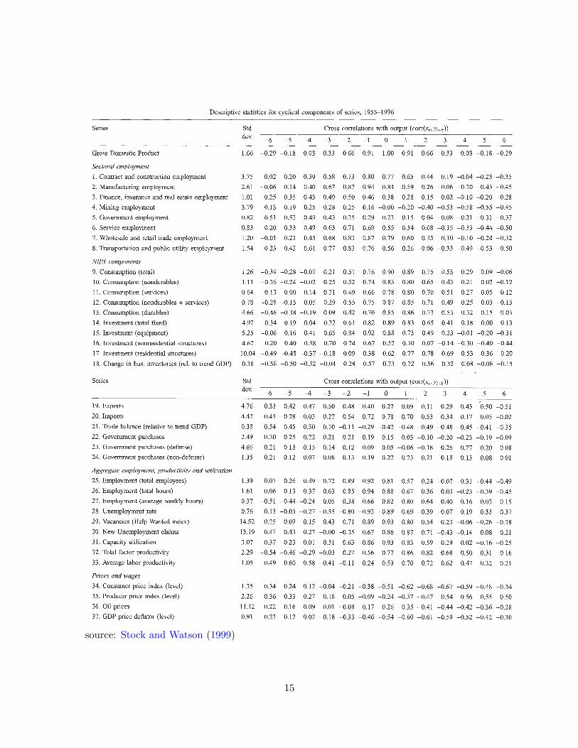
source: Stock and Watson (1999)

15

source: Stock and Watson (1999)

16