introduction to matlab - halvorsen.blog...matlab course - part i: introduction to matlab matlab...
TRANSCRIPT
Introduction to MATLAB
Hans-Petter Halvorsen
https://www.halvorsen.blog

Introduction to MATLAB
University of South-Eastern Norway
MATLAB Introduction to MATLAB
Hans-Petter Halvorsen, 2019.08.06
http://www.halvorsen.blog
ii
Preface
Copyright You cannot distribute or copy this document without
permission from the author. You cannot copy or link to this document
directly from other sources, web pages, etc. You should always link to the
proper web page where this document is located, typically
http://www.halvorsen.blog
In this MATLAB Course, you will learn basic MATLAB and how to use
MATLAB in Control and Simulation applications. An introduction to
Simulink and other Tools will also be given.
MATLAB is a tool for technical computing, computation and visualization in
an integrated environment. MATLAB is an abbreviation for MATrix
LABoratory, so it is well suited for matrix manipulation and problem
solving related to Linear Algebra, Modelling, Simulation and Control
applications.
This is a self-paced course based on this document and some short videos
on the way. This document contains lots of examples and self-paced tasks
that the users will go through and solve on their own. The user may go
through the tasks in this document in their own pace and the instructor
will be available for guidance throughout the course.
The MATLAB Course consists of 3 parts:
1. Introduction to MATLAB
2. Modelling, Simulation and Control
3. Simulink and Advanced Topics
In part 1 you will be familiar with the MATLAB environment and learn
basic MATLAB programming.
The course consists of lots of Tasks you should solve while reading this
course manual and watching the videos referred to in the text.
iii
Make sure to bring your headphones for the videos in this
course. The course consists of several short videos that will give you an
introduction to the different topics in the course.
Prerequisites
You should be familiar with undergraduate-level mathematics and have
experience with basic computer operations.
What is MATLAB? MATLAB is a tool for technical computing, computation
and visualization in an integrated environment. MATLAB is an abbreviation
for MATrix LABoratory, so it is well suited for matrix manipulation and
problem solving related to Linear Algebra.
MATLAB is developed by The MathWorks. MATLAB is a short-term for
MATrix LABoratory. MATLAB is in use world-wide by researchers and
universities. For more information, see www.mathworks.com
For more information about MATLAB, etc., please visit
http://www.halvorsen.blog
Online MATLAB Resources:
MATLAB:
http://www.halvorsen.blog/documents/programming/matlab/
MATLAB Basics:
http://www.halvorsen.blog/documents/programming/matlab/matlab_basi
cs.php
Modelling, Simulation and Control with MATLAB:
http://www.halvorsen.blog/documents/programming/matlab/matlab_mic.
php
iv
MATLAB Videos:
http://www.halvorsen.blog/documents/video/matlab_basics_videos.php
MATLAB for Students:
http://www.halvorsen.blog/documents/teaching/courses/matlab.php
On these web pages you find video solutions, complete step by step
solutions, downloadable MATLAB code, additional resources, etc.
v
Table of Contents
Preface ............................................................................................ ii
Table of Contents .............................................................................. v
1 Introduction ............................................................................... 1
2 The MATLAB Environment ............................................................ 2
2.1 Command Window ................................................................. 3
2.2 Command History .................................................................. 4
2.3 Workspace ............................................................................ 4
2.4 Current Folder ....................................................................... 6
2.5 Editor ................................................................................... 7
3 Using the Help System in MATLAB ................................................. 9
4 MATLAB Basics .......................................................................... 11
4.1 Basic Operations .................................................................. 11
Task 1: Basic Operations ......................................................... 13
Task 2: Statistics functions ...................................................... 15
4.2 Arrays; Vectors and Matrices ................................................. 16
4.2.1 Colon Notation ............................................................... 17
Task 3: Vectors and Matrices .................................................... 18
4.3 Tips and Tricks .................................................................... 19
4.3.1 Array Operations ............................................................ 20
5 Linear Algebra; Vectors and Matrices ........................................... 23
5.1 Vectors ............................................................................... 23
5.2 Matrices ............................................................................. 26
5.2.1 Transpose ..................................................................... 26
vi Table of Contents
MATLAB Course - Part I: Introduction to MATLAB
5.2.2 Diagonal ....................................................................... 26
5.2.3 Triangular ..................................................................... 27
5.2.4 Matrix Multiplication ....................................................... 28
5.2.5 Matrix Addition .............................................................. 29
5.2.6 Determinant .................................................................. 29
5.2.7 Inverse Matrices ............................................................ 30
5.3 Eigenvalues ........................................................................ 31
Task 4: Matrix manipulation ..................................................... 32
5.4 Solving Linear Equations ....................................................... 32
Task 5: Solving Linear Equations .............................................. 34
6 M-files; Scripts and user-define functions ..................................... 35
6.1 Scripts vs. function Files ....................................................... 35
6.2 Scripts ............................................................................... 36
Task 6: Script ......................................................................... 38
6.3 Functions ............................................................................ 39
Task 7: User-defined function ................................................... 42
Task 8: User-defined function ................................................... 42
7 Plotting .................................................................................... 44
Task 9: Plotting ...................................................................... 45
7.1 Plotting Multiple Data Sets in One Graph ................................ 46
Task 10: Plot of dynamic system ............................................. 49
7.2 Displaying Multiple Plots in one Figure – Sub-Plots ................... 50
Task 11: Sub-plots ................................................................. 51
7.3 Custimizing ......................................................................... 51
7.4 Other Plots ......................................................................... 55
Task 12: Other Plots .............................................................. 55
vii Table of Contents
MATLAB Course - Part I: Introduction to MATLAB
8 Flow Control and Loops .............................................................. 56
8.1 Introduction ........................................................................ 56
8.2 If-else Statement ................................................................ 56
Task 13: If-else Statements .................................................... 58
8.3 Switch and Case Statement .................................................. 59
Task 14: Switch-Case Statements ............................................ 59
8.4 For loop .............................................................................. 60
Task 15: Fibonacci Numbers.................................................... 60
8.5 While loop .......................................................................... 61
Task 16: While Loop ............................................................... 62
8.6 Additional Tasks .................................................................. 62
Task 17: For Loops ................................................................ 62
Task 18: If-else Statement ..................................................... 63
9 Mathematics ............................................................................. 64
9.1 Basic Math Functions ............................................................ 64
Task 19: Basic Math function ................................................... 64
9.2 Statistics ............................................................................ 64
Task 20: Statistics ................................................................. 64
9.3 Trigonometric Functions ....................................................... 65
Task 21: Conversion .............................................................. 65
Task 22: Trigonometric functions on right triangle ..................... 65
Task 23: Law of cosines .......................................................... 67
Task 24: Plotting ................................................................... 67
9.4 Complex Numbers ............................................................... 67
Task 25: Complex numbers ..................................................... 71
Task 26: Complex numbers ..................................................... 71
viii Table of Contents
MATLAB Course - Part I: Introduction to MATLAB
9.5 Polynomials ........................................................................ 71
Task 27: Polynomials ............................................................. 72
Task 28: Polynomials ............................................................. 72
Task 29: Polynomial Fitting ..................................................... 73
10 Additional Tasks ..................................................................... 74
Task 30: User-defined function ................................................ 74
Task 31: MATLAB Script.......................................................... 74
Task 32: Cylinder surface area ................................................ 75
Task 33: Create advanced expressions in MATLAB ..................... 75
Task 34: Solving Equations ..................................................... 76
Task 35: Pre-allocating of variables and vectorization ................. 76
Task 36: Nested For Loops ...................................................... 78
Appendix A: MATLAB Functions......................................................... 81
Built-in Constants ........................................................................ 81
Basic Functions ............................................................................ 81
Linear Algebra ............................................................................. 82
Plotting ....................................................................................... 82
Logical Operators ......................................................................... 83
Complex Numbers ........................................................................ 83
1
1 Introduction
Additional Resources, Videos, etc. are available from:
http://www.halvorsen.blog/documents/programming/matlab
Part I: Introduction to MATLAB consists of the following topics:
• The MATLAB Environment
• Using the Help System in MATLAB
• MATLAB Basics
• Linear Algebra; Vectors and Matrices
• M files; Scripts and User-defined functions
• Plotting
• Flow Control and Loops; For and While Loops, If and Case
statements
• Mathematics
• Additional Tasks
2
2 The MATLAB
Environment
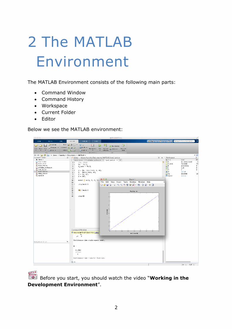
The MATLAB Environment consists of the following main parts:
• Command Window
• Command History
• Workspace
• Current Folder
• Editor
Below we see the MATLAB environment:
Before you start, you should watch the video “Working in the
Development Environment”.
3 The MATLAB Environment
MATLAB Course - Part I: Introduction to MATLAB
The video is available from:
https://www.halvorsen.blog/documents/teaching/courses/matlab/matlab1
.php
2.1 Command Window
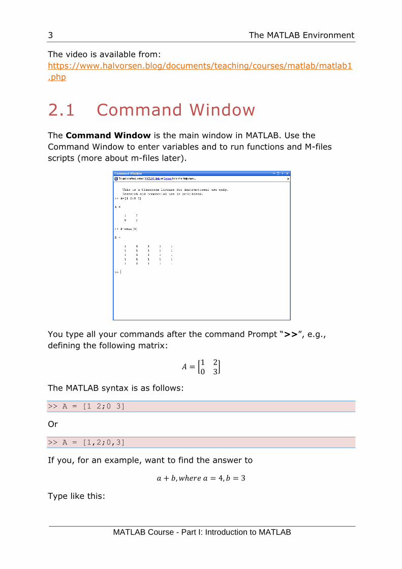
The Command Window is the main window in MATLAB. Use the
Command Window to enter variables and to run functions and M-files
scripts (more about m-files later).
You type all your commands after the command Prompt “>>”, e.g.,
defining the following matrix:
𝐴 = [1 20 3
]
The MATLAB syntax is as follows:
>> A = [1 2;0 3]
Or
>> A = [1,2;0,3]
If you, for an example, want to find the answer to
𝑎 + 𝑏,𝑤ℎ𝑒𝑟𝑒 𝑎 = 4, 𝑏 = 3
Type like this:
4 The MATLAB Environment
MATLAB Course - Part I: Introduction to MATLAB
>>a = 4
>>b = 3
>>a + b
MATLAB then responds:
ans =
7
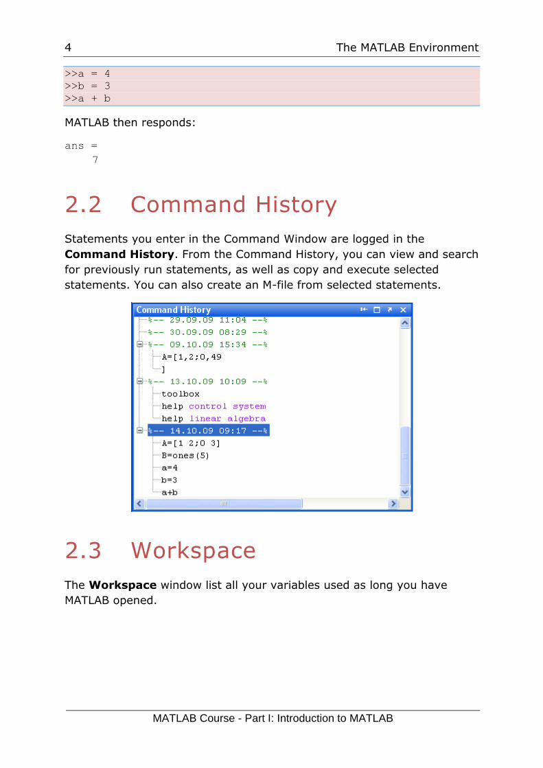
2.2 Command History
Statements you enter in the Command Window are logged in the
Command History. From the Command History, you can view and search
for previously run statements, as well as copy and execute selected
statements. You can also create an M-file from selected statements.
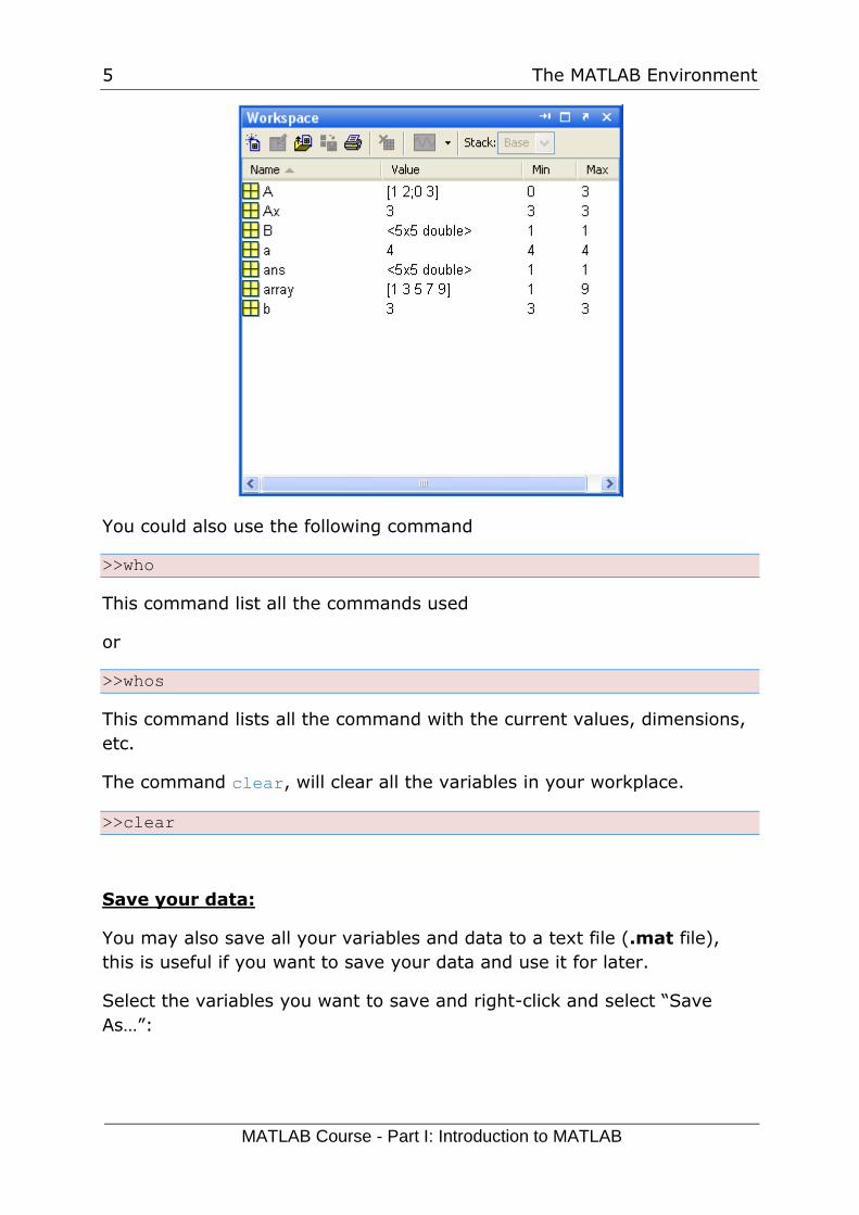
2.3 Workspace
The Workspace window list all your variables used as long you have
MATLAB opened.
5 The MATLAB Environment
MATLAB Course - Part I: Introduction to MATLAB
You could also use the following command
>>who
This command list all the commands used
or
>>whos
This command lists all the command with the current values, dimensions,
etc.
The command clear, will clear all the variables in your workplace.
>>clear
Save your data:
You may also save all your variables and data to a text file (.mat file),
this is useful if you want to save your data and use it for later.
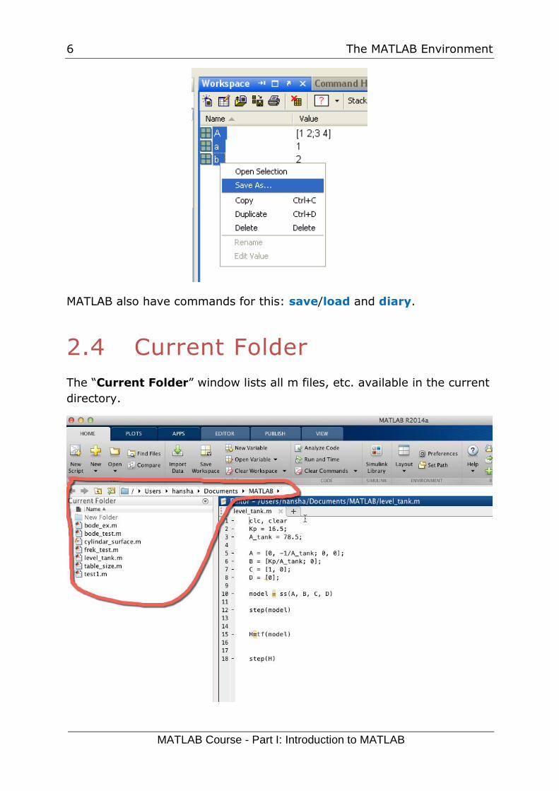
Select the variables you want to save and right-click and select “Save
As…”:
6 The MATLAB Environment
MATLAB Course - Part I: Introduction to MATLAB
MATLAB also have commands for this: save/load and diary.
2.4 Current Folder
The “Current Folder” window lists all m files, etc. available in the current
directory.
7 The MATLAB Environment
MATLAB Course - Part I: Introduction to MATLAB
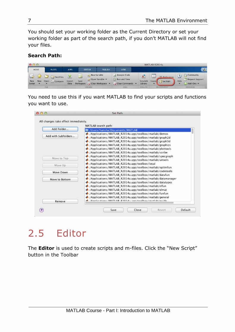
You should set your working folder as the Current Directory or set your
working folder as part of the search path, if you don’t MATLAB will not find
your files.
Search Path:
You need to use this if you want MATLAB to find your scripts and functions
you want to use.
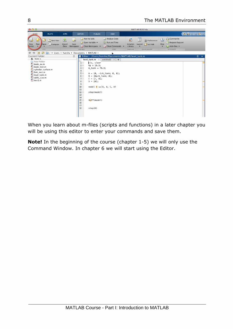
2.5 Editor
The Editor is used to create scripts and m-files. Click the “New Script”
button in the Toolbar
8 The MATLAB Environment
MATLAB Course - Part I: Introduction to MATLAB
When you learn about m-files (scripts and functions) in a later chapter you
will be using this editor to enter your commands and save them.
Note! In the beginning of the course (chapter 1-5) we will only use the
Command Window. In chapter 6 we will start using the Editor.
9
3 Using the Help
System in MATLAB
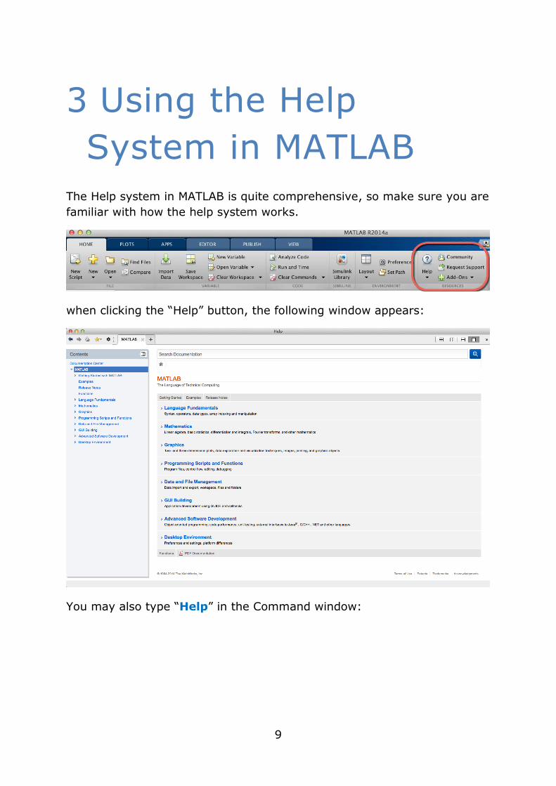
The Help system in MATLAB is quite comprehensive, so make sure you are
familiar with how the help system works.
when clicking the “Help” button, the following window appears:
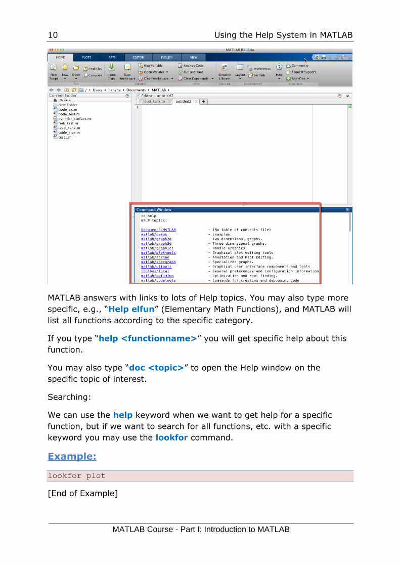
You may also type “Help” in the Command window:
10 Using the Help System in MATLAB
MATLAB Course - Part I: Introduction to MATLAB
MATLAB answers with links to lots of Help topics. You may also type more
specific, e.g., “Help elfun” (Elementary Math Functions), and MATLAB will
list all functions according to the specific category.
If you type “help <functionname>” you will get specific help about this
function.
You may also type “doc <topic>” to open the Help window on the
specific topic of interest.
Searching:
We can use the help keyword when we want to get help for a specific
function, but if we want to search for all functions, etc. with a specific
keyword you may use the lookfor command.
Example:
lookfor plot
[End of Example]
11
4 MATLAB Basics
Before you start, you should watch the video “Getting Started with
MATLAB”
The video is available from:
https://www.halvorsen.blog/documents/teaching/courses/matlab/matlab1
.php
4.1 Basic Operations
Variables:
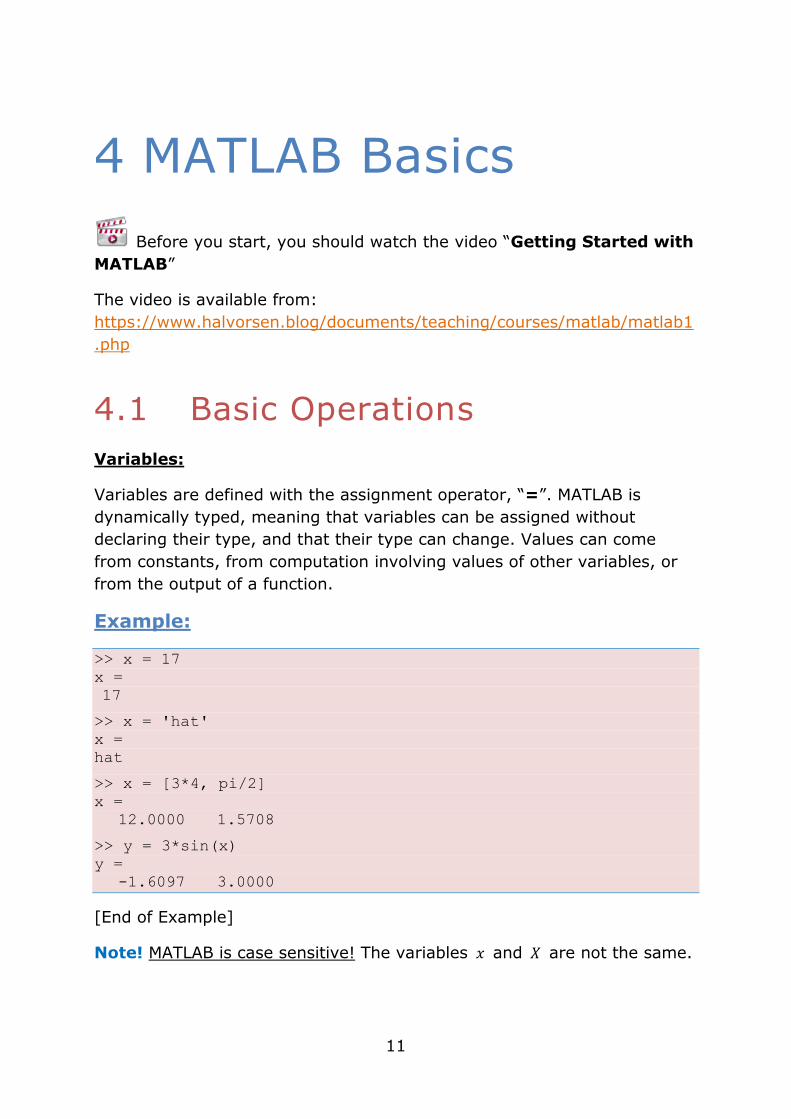
Variables are defined with the assignment operator, “=”. MATLAB is
dynamically typed, meaning that variables can be assigned without
declaring their type, and that their type can change. Values can come
from constants, from computation involving values of other variables, or
from the output of a function.
Example:
>> x = 17
x =
17
>> x = 'hat'
x =
hat
>> x = [3*4, pi/2]
x =
12.0000 1.5708
>> y = 3*sin(x)
y =
-1.6097 3.0000
[End of Example]
Note! MATLAB is case sensitive! The variables 𝑥 and 𝑋 are not the same.
12 MATLAB Basics
MATLAB Course - Part I: Introduction to MATLAB
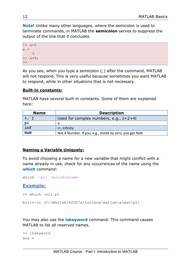
Note! Unlike many other languages, where the semicolon is used to
terminate commands, in MATLAB the semicolon serves to suppress the
output of the line that it concludes.
>> a=5
a =
5
>> a=6;
>>
As you see, when you type a semicolon (;) after the command, MATLAB
will not respond. This is very useful because sometimes you want MATLAB
to respond, while in other situations that is not necessary.
Built-in constants:
MATLAB have several built-in constants. Some of them are explained
here:
Name Description
i, j Used for complex numbers, e.g., z=2+4i pi 𝜋 inf ∞, Infinity NaN Not A Number. If you, e.g., divide by zero, you get NaN
Naming a Variable Uniquely:
To avoid choosing a name for a new variable that might conflict with a
name already in use, check for any occurrences of the name using the
which command:
which -all variablename
Example:
>> which -all pi
built-in (C:\Matlab\R2007a\toolbox\matlab\elmat\pi)
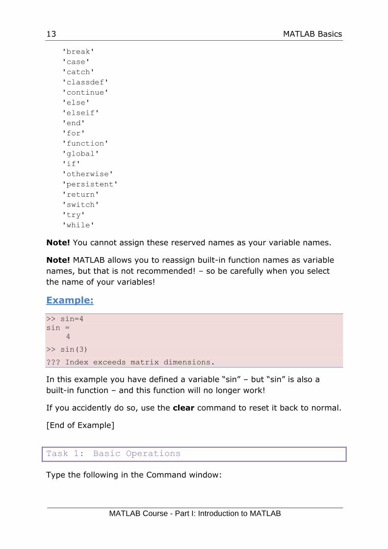
You may also use the iskeyword command. This command causes
MATLAB to list all reserved names.
>> iskeyword
ans =
13 MATLAB Basics
MATLAB Course - Part I: Introduction to MATLAB
'break'
'case'
'catch'
'classdef'
'continue'
'else'
'elseif'
'end'
'for'
'function'
'global'
'if'
'otherwise'
'persistent'
'return'
'switch'
'try'
'while'
Note! You cannot assign these reserved names as your variable names.
Note! MATLAB allows you to reassign built-in function names as variable
names, but that is not recommended! – so be carefully when you select
the name of your variables!
Example:
>> sin=4
sin =
4
>> sin(3)
??? Index exceeds matrix dimensions.
In this example you have defined a variable “sin” – but “sin” is also a
built-in function – and this function will no longer work!
If you accidently do so, use the clear command to reset it back to normal.
[End of Example]
Task 1: Basic Operations
Type the following in the Command window:
14 MATLAB Basics
MATLAB Course - Part I: Introduction to MATLAB
>>y=16;
>>z=3;
>>y+z
Note! When you use a semicolon, no output will be displayed. Try the
code above with and without semicolon.
Note! Some functions display output even if you use semicolon, like plot,
etc.
Other basic operations are:
>>16-3
>>16/3
>>16*3
→ Try them.
[End of Task]
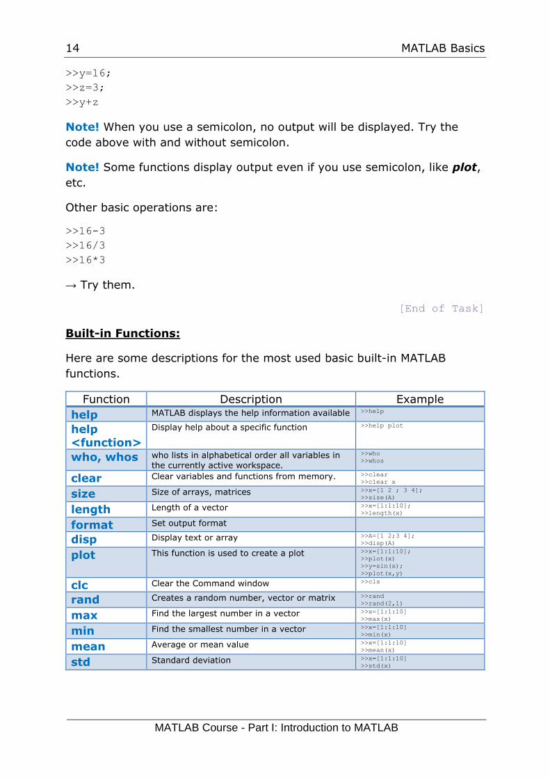
Built-in Functions:
Here are some descriptions for the most used basic built-in MATLAB
functions.
Function Description Example
help MATLAB displays the help information available >>help
help <function>
Display help about a specific function >>help plot
who, whos who lists in alphabetical order all variables in the currently active workspace.
>>who
>>whos
clear Clear variables and functions from memory. >>clear
>>clear x
size Size of arrays, matrices >>x=[1 2 ; 3 4];
>>size(A)
length Length of a vector >>x=[1:1:10];
>>length(x)
format Set output format
disp Display text or array >>A=[1 2;3 4];
>>disp(A)
plot This function is used to create a plot >>x=[1:1:10];
>>plot(x)
>>y=sin(x);
>>plot(x,y)
clc Clear the Command window >>cls
rand Creates a random number, vector or matrix >>rand
>>rand(2,1)
max Find the largest number in a vector >>x=[1:1:10]
>>max(x)
min Find the smallest number in a vector >>x=[1:1:10]
>>min(x)
mean Average or mean value >>x=[1:1:10]
>>mean(x)
std Standard deviation >>x=[1:1:10]
>>std(x)
15 MATLAB Basics
MATLAB Course - Part I: Introduction to MATLAB
Before you start, you should use the Help system in MATLAB to read more
about these functions. Type “help <functionname>” in the Command
window.
Task 2: Statistics functions
Create a random vector with 100 random numbers between 0 and 100.
Find the minimum value, the maximum value, the mean and the standard
deviation using some of the built-in functions in MATLAB listed above.
[End of Task]
16 MATLAB Basics
MATLAB Course - Part I: Introduction to MATLAB
4.2 Arrays; Vectors and Matrices
Before you start, you should watch the video “Working with
Arrays”.
The video is available from:
https://www.halvorsen.blog/documents/teaching/courses/matlab/matlab1
.php
Matrices and vectors (Linear Algebra) are the basic elements in MATLAB
and also the basic elements in control design theory. So it is important
you know how to handle vectors and matrices in MATLAB.
A general matrix 𝐴 may be written like this:
𝐴 = [
𝑎11 ⋯ 𝑎1𝑚⋮ ⋱ ⋮𝑎𝑛1 ⋯ 𝑎𝑛𝑚
] ∈ 𝑅𝑛𝑥𝑚
In MATLAB we type vectors and matrices like this:
𝐴 = [1 23 4
]
>> A = [1 2; 3 4]
A = 1 2
3 4
or:
>> A = [1, 2; 3, 4]
A = 1 2
3 4
→ To separate rows, we use a semicolon “;”
→ To separate columns, we use a comma “,” or a space “ “.
To get a specific part of a matrix, we can type like this:
>> A(2,1)
ans =
3
or:
17 MATLAB Basics
MATLAB Course - Part I: Introduction to MATLAB
>> A(:,1)
ans =
1
3
or:
>> A(2,:)
ans =
3 4
From 2 vectors x and y we can create a matrix like this:
>> x = [1; 2; 3];
>> y = [4; 5; 6];
>> B = [x y]
B = 1 4
2 5
3 6
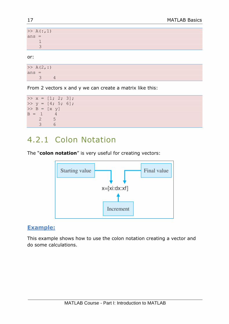
4.2.1 Colon Notation
The “colon notation” is very useful for creating vectors:
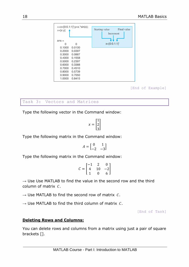
Example:
This example shows how to use the colon notation creating a vector and
do some calculations.
18 MATLAB Basics
MATLAB Course - Part I: Introduction to MATLAB
[End of Example]
Task 3: Vectors and Matrices
Type the following vector in the Command window:
𝑥 = [123]
Type the following matrix in the Command window:
𝐴 = [0 1−2 −3
]
Type the following matrix in the Command window:
𝐶 = [−1 2 04 10 −21 0 6
]
→ Use Use MATLAB to find the value in the second row and the third
column of matrix 𝐶.
→ Use MATLAB to find the second row of matrix 𝐶.
→ Use MATLAB to find the third column of matrix 𝐶.
[End of Task]
Deleting Rows and Columns:
You can delete rows and columns from a matrix using just a pair of square
brackets [].
19 MATLAB Basics
MATLAB Course - Part I: Introduction to MATLAB
Example:
Given:
𝐴 = [0 1−2 −3
]
To delete the second column of a matrix 𝐴, use:
>>A=[0 1; -2 -3];
>>A(:,2) = []
A =
0
-2
[End of Example]
4.3 Tips and Tricks
Naming conversions:
When creating variables and constants, make sure you create a name that
is not already exists in MATLAB. Note also that MATLAB is case sensitive!
The variables x and X are not the same.
Use the which command to check if the name already exists: which –all
<your name>
Example:
>> which -all sin
built-in (C:\Matlab\R2007a\toolbox\matlab\elfun\@double\sin) %
double method
built-in (C:\Matlab\R2007a\toolbox\matlab\elfun\@single\sin) %
single method
Large or small numbers:
If you need to write large or small numbers, like 2 𝑥 105 , 7.5 𝑥 10−8you can
use the “e” notation, e.g.:
>> 2e5
ans =
20 MATLAB Basics
MATLAB Course - Part I: Introduction to MATLAB
200000
>> 7.5e-8
ans =
7.5000e-008
Line Continuation:
For large arrays, it may be difficult to fit one row on one command line.
We may then split the row across several command lines by using the line
continuation operator “...”.
Example:
>> x=[1 2 3 4 5 ...
6 7 8 9 10]
x =
1 2 3 4 5 6 7 8 9 10
Multiple commands on same line:
It is possible to type several commands on the same line. In some cases
this is a good idea to save space.
Example:
>> x=1,y=2,z=3
x =
1
y =
2
z =
3
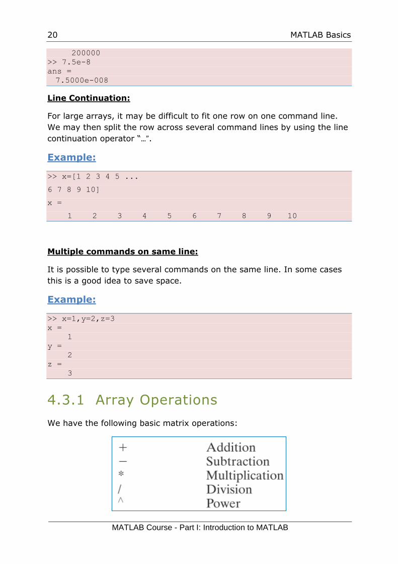
4.3.1 Array Operations
We have the following basic matrix operations:
21 MATLAB Basics
MATLAB Course - Part I: Introduction to MATLAB
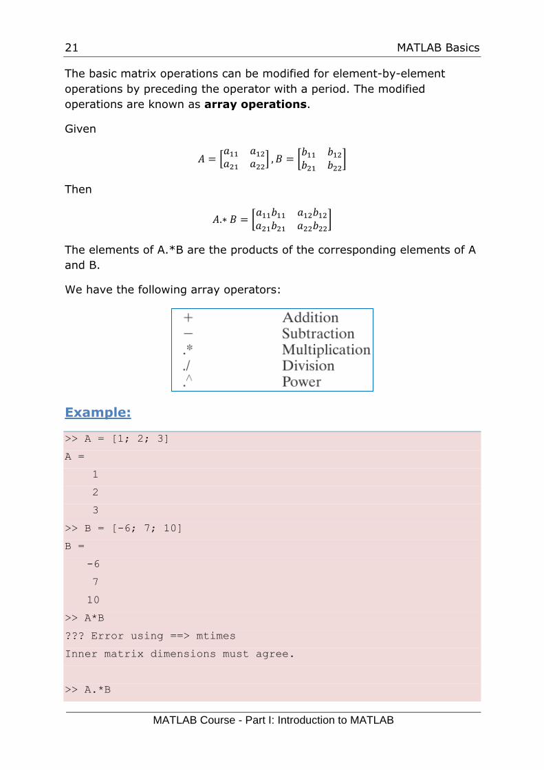
The basic matrix operations can be modified for element-by-element
operations by preceding the operator with a period. The modified
operations are known as array operations.
Given
𝐴 = [𝑎11 𝑎12𝑎21 𝑎22
] , 𝐵 = [𝑏11 𝑏12𝑏21 𝑏22
]
Then
𝐴.∗ 𝐵 = [𝑎11𝑏11 𝑎12𝑏12𝑎21𝑏21 𝑎22𝑏22
]
The elements of A.*B are the products of the corresponding elements of A
and B.
We have the following array operators:
Example:
>> A = [1; 2; 3]
A =
1
2
3
>> B = [-6; 7; 10]
B =
-6
7
10
>> A*B
??? Error using ==> mtimes
Inner matrix dimensions must agree.
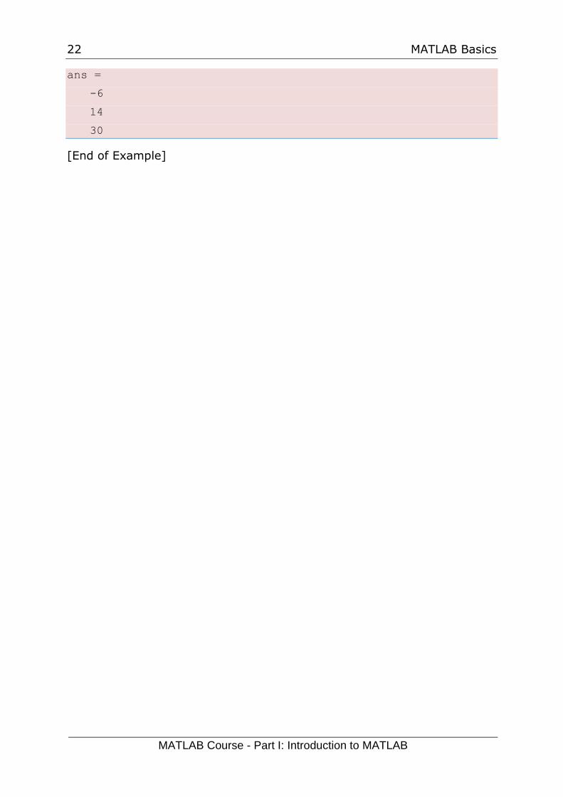
>> A.*B
22 MATLAB Basics
MATLAB Course - Part I: Introduction to MATLAB
ans =
-6
14
30
[End of Example]
23
5 Linear Algebra;
Vectors and Matrices
Linear Algebra is a branch of mathematics concerned with the study of
matrices, vectors, vector spaces (also called linear spaces), linear maps
(also called linear transformations), and systems of linear equations.
MATLAB are well suited for Linear Algebra. This chapter assumes you have
some basic understanding of Linear Algebra and matrices and vectors.
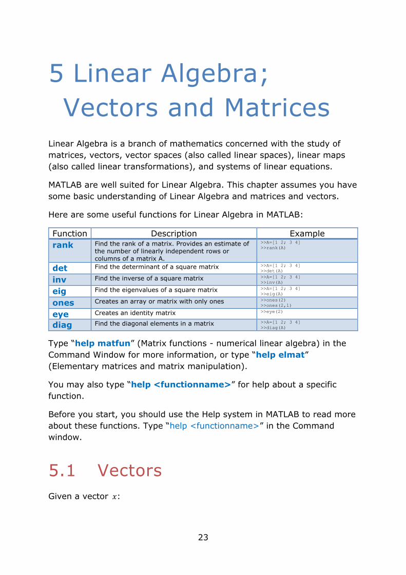
Here are some useful functions for Linear Algebra in MATLAB:
Function Description Example
rank Find the rank of a matrix. Provides an estimate of the number of linearly independent rows or columns of a matrix A.
>>A=[1 2; 3 4]
>>rank(A)
det Find the determinant of a square matrix >>A=[1 2; 3 4]
>>det(A)
inv Find the inverse of a square matrix >>A=[1 2; 3 4]
>>inv(A)
eig Find the eigenvalues of a square matrix >>A=[1 2; 3 4]
>>eig(A)
ones Creates an array or matrix with only ones >>ones(2)
>>ones(2,1)
eye Creates an identity matrix >>eye(2)
diag Find the diagonal elements in a matrix >>A=[1 2; 3 4]
>>diag(A)
Type “help matfun” (Matrix functions - numerical linear algebra) in the
Command Window for more information, or type “help elmat”
(Elementary matrices and matrix manipulation).
You may also type “help <functionname>” for help about a specific
function.
Before you start, you should use the Help system in MATLAB to read more
about these functions. Type “help <functionname>” in the Command
window.
5.1 Vectors
Given a vector 𝑥:
24 Linear Algebra; Vectors and Matrices
MATLAB Course - Part I: Introduction to MATLAB
𝑥 = [
𝑥1𝑥2⋮𝑥𝑛
] ∈ 𝑅𝑛
Example:
Given:
𝑥 = [123]
>> x=[1; 2; 3]
x =
1
2
3
The Transpose of vector x:
𝑥𝑇 = [𝑥1 𝑥2 ⋯ 𝑥𝑛] ∈ 𝑅1𝑥𝑛
>> x'
ans =
1 2 3
[End of Example]
The Length of vector x:
‖𝑥‖ = √𝑥𝑇𝑥 = √𝑥12 + 𝑥2
2 +⋯+ 𝑥𝑛2
Example:
The length of a vector most makes sense for 2 or 3 dimensional vectors.
Given the following vector:
𝑣 = [3, 4]
Note! Sometimes you also see it like this: �⃑�
25 Linear Algebra; Vectors and Matrices
MATLAB Course - Part I: Introduction to MATLAB
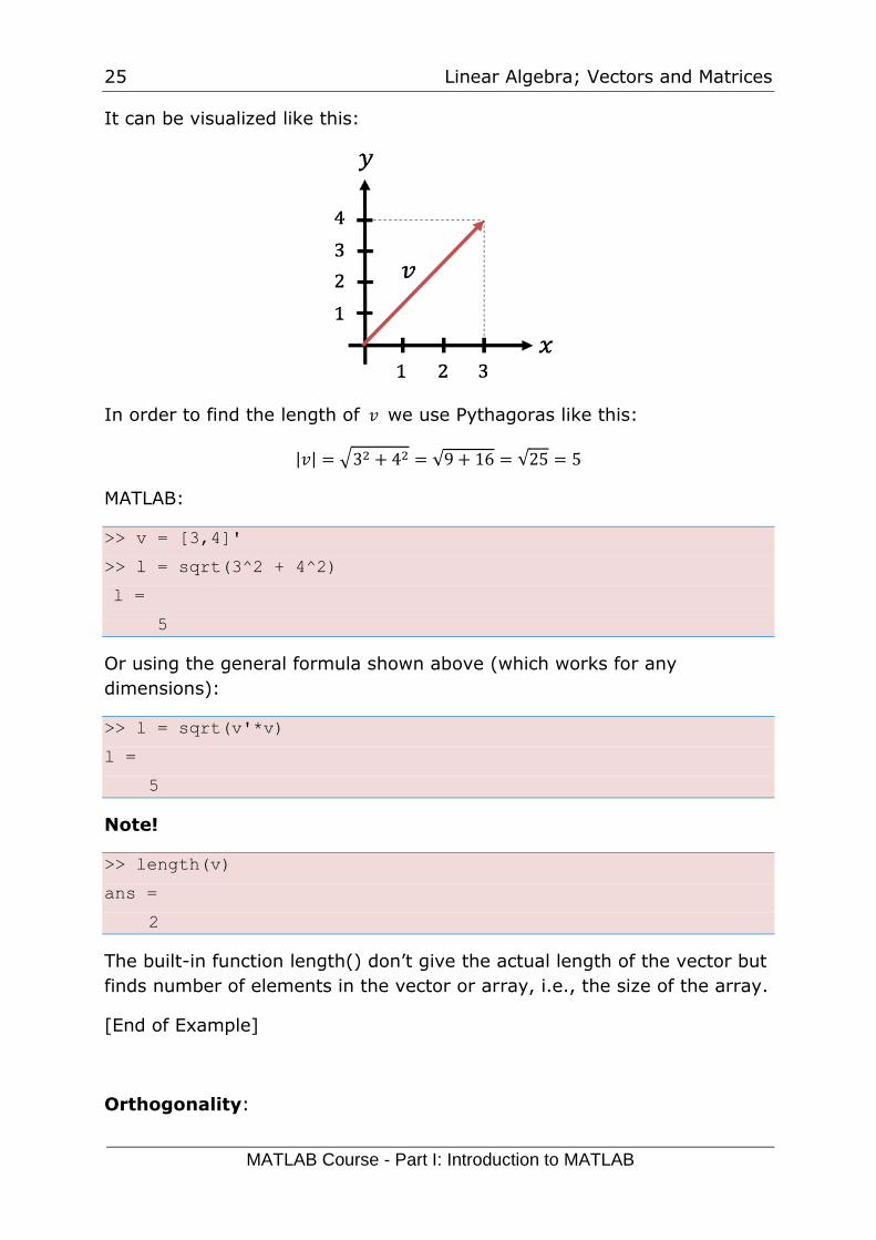
It can be visualized like this:
In order to find the length of 𝑣 we use Pythagoras like this:
|𝑣| = √32 + 42 = √9 + 16 = √25 = 5
MATLAB:
>> v = [3,4]'
>> l = sqrt(3^2 + 4^2)
l =
5
Or using the general formula shown above (which works for any
dimensions):
>> l = sqrt(v'*v)
l =
5
Note!
>> length(v)
ans =
2
The built-in function length() don’t give the actual length of the vector but
finds number of elements in the vector or array, i.e., the size of the array.
[End of Example]
Orthogonality:
26 Linear Algebra; Vectors and Matrices
MATLAB Course - Part I: Introduction to MATLAB
𝑥𝑇𝑦 = 0
5.2 Matrices
Given a matrix 𝐴:
𝐴 = [
𝑎11 ⋯ 𝑎1𝑚⋮ ⋱ ⋮𝑎𝑛1 ⋯ 𝑎𝑛𝑚
] ∈ 𝑅𝑛𝑥𝑚
Example:
𝐴 = [0 1−2 −3
]
>> A=[0 1;-2 -3]
A =
0 1
-2 -3
[End of Example]
5.2.1 Transpose
The Transpose of matrix 𝐴:
𝐴𝑇 = [
𝑎11 ⋯ 𝑎𝑛1⋮ ⋱ ⋮𝑎1𝑚 ⋯ 𝑎𝑛𝑚
] ∈ 𝑅𝑚𝑥𝑛
Example:
𝐴𝑇 = [0 1−2 −3
]𝑇
= [0 −21 −3
]
>> A'
ans =
0 -2
1 -3
[End of Example]
5.2.2 Diagonal
The Diagonal elements of matrix A is the vector
27 Linear Algebra; Vectors and Matrices
MATLAB Course - Part I: Introduction to MATLAB
𝑑𝑖𝑎𝑔(𝐴) = [
𝑎11𝑎22⋮𝑎𝑝𝑝
] ∈ 𝑅𝑝=min (𝑥,𝑚)
Example:
>> diag(A)
ans =
0
-3
[End of Example]
The Diagonal matrix Λ is given by:
Λ = [
𝜆1 0 ⋯ 00 𝜆2 ⋯ 0⋮ ⋮ ⋱ ⋮0 0 ⋯ 𝜆𝑛
] ∈ 𝑅𝑛𝑥𝑛
Given the Identity matrix I:
𝐼 = [
1 0 ⋯ 00 1 ⋯ 0⋮ ⋮ ⋱ ⋮0 0 ⋯ 1
] ∈ 𝑅𝑛𝑥𝑚
Example:
>> eye(3)
ans =
1 0 0
0 1 0
0 0 1
[End of Example]
5.2.3 Triangular
Lower Triangular matrix L:
𝐿 = [. 0 0⋮ ⋱ 0. ⋯ .
]
28 Linear Algebra; Vectors and Matrices
MATLAB Course - Part I: Introduction to MATLAB
Upper Triangular matrix U:
𝑈 = [
. ⋯ .0 ⋱ ⋮0 0 .
]
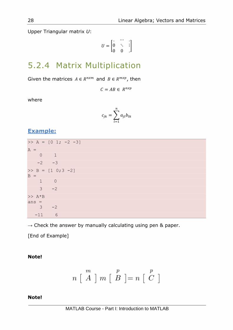
5.2.4 Matrix Multiplication
Given the matrices 𝐴 ∈ 𝑅𝑛𝑥𝑚 and 𝐵 ∈ 𝑅𝑚𝑥𝑝, then
𝐶 = 𝐴𝐵 ∈ 𝑅𝑛𝑥𝑝
where
𝑐𝑗𝑘 =∑𝑎𝑗𝑙𝑏𝑙𝑘
𝑛
𝑙=1
Example:
>> A = [0 1; -2 -3]
A =
0 1
-2 -3
>> B = [1 0;3 -2]
B =
1 0
3 -2
>> A*B
ans =
3 -2
-11 6
→ Check the answer by manually calculating using pen & paper.
[End of Example]
Note!
Note!
29 Linear Algebra; Vectors and Matrices
MATLAB Course - Part I: Introduction to MATLAB
𝐴𝐵 ≠ 𝐵𝐴
𝐴(𝐵𝐶) = (𝐴𝐵)𝐶
(𝐴 + 𝐵)𝐶 = 𝐴𝐶 + 𝐵𝐶
𝐶(𝐴 + 𝐵) = 𝐶𝐴 + 𝐶𝐵
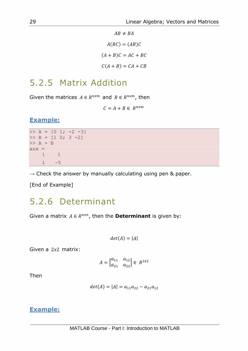
5.2.5 Matrix Addition
Given the matrices 𝐴 ∈ 𝑅𝑛𝑥𝑚 and 𝐵 ∈ 𝑅𝑛𝑥𝑚, then
𝐶 = 𝐴 + 𝐵 ∈ 𝑅𝑛𝑥𝑚
Example:
>> A = [0 1; -2 -3]
>> B = [1 0; 3 -2]
>> A + B
ans =
1 1
1 -5
→ Check the answer by manually calculating using pen & paper.
[End of Example]
5.2.6 Determinant
Given a matrix 𝐴 ∈ 𝑅𝑛𝑥𝑛, then the Determinant is given by:
𝑑𝑒𝑡(𝐴) = |𝐴|
Given a 2𝑥2 matrix:
𝐴 = [𝑎11 𝑎12𝑎21 𝑎22
] ∈ 𝑅2𝑥2
Then
𝑑𝑒𝑡(𝐴) = |𝐴| = 𝑎11𝑎22 − 𝑎21𝑎12
Example:
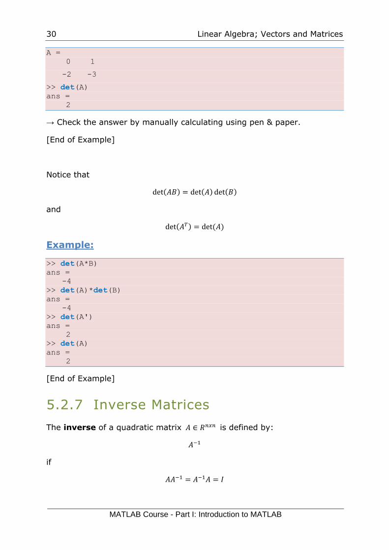
30 Linear Algebra; Vectors and Matrices
MATLAB Course - Part I: Introduction to MATLAB
A =
0 1
-2 -3
>> det(A)
ans =
2
→ Check the answer by manually calculating using pen & paper.
[End of Example]
Notice that
det(𝐴𝐵) = det(𝐴) det(𝐵)
and
det(𝐴𝑇) = det (𝐴)
Example:
>> det(A*B)
ans =
-4
>> det(A)*det(B)
ans =
-4
>> det(A')
ans =
2
>> det(A)
ans =
2
[End of Example]
5.2.7 Inverse Matrices
The inverse of a quadratic matrix 𝐴 ∈ 𝑅𝑛𝑥𝑛 is defined by:
𝐴−1
if
𝐴𝐴−1 = 𝐴−1𝐴 = 𝐼
31 Linear Algebra; Vectors and Matrices
MATLAB Course - Part I: Introduction to MATLAB
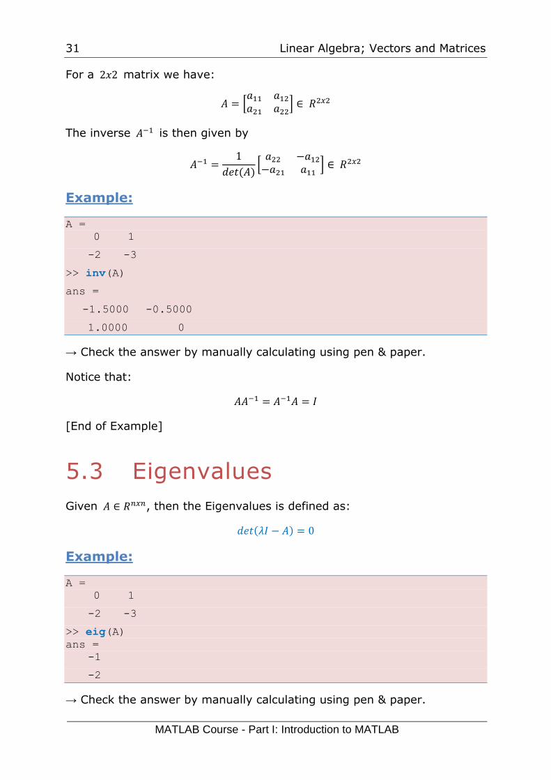
For a 2𝑥2 matrix we have:
𝐴 = [𝑎11 𝑎12𝑎21 𝑎22
] ∈ 𝑅2𝑥2
The inverse 𝐴−1 is then given by
𝐴−1 =1
𝑑𝑒𝑡 (𝐴)[𝑎22 −𝑎12−𝑎21 𝑎11
] ∈ 𝑅2𝑥2
Example:
A =
0 1
-2 -3
>> inv(A)
ans =
-1.5000 -0.5000
1.0000 0
→ Check the answer by manually calculating using pen & paper.
Notice that:
𝐴𝐴−1 = 𝐴−1𝐴 = 𝐼
[End of Example]
5.3 Eigenvalues
Given 𝐴 ∈ 𝑅𝑛𝑥𝑛, then the Eigenvalues is defined as:
𝑑𝑒𝑡(𝜆𝐼 − 𝐴) = 0
Example:
A =
0 1
-2 -3
>> eig(A)
ans =
-1
-2
→ Check the answer by manually calculating using pen & paper.
32 Linear Algebra; Vectors and Matrices
MATLAB Course - Part I: Introduction to MATLAB
[End of Example]
Task 4: Matrix manipulation
In this task we will practice on entering matrices and perform basic matrix
operations.
Given the matrices 𝐴, 𝐵 and 𝐶:
𝐴 = [0 1−2 −3
] , 𝐵 = [1 03 −2
] , 𝐶 = [1 −1−2 2
]
→ Solve the following basic matrix operations using MATLAB:
• 𝐴 + 𝐵
• 𝐴 − 𝐵
• 𝐴𝑇
• 𝐴−1
• 𝑑𝑖𝑎𝑔(𝐴), 𝑑𝑖𝑎𝑔(𝐵)
• 𝑑𝑒𝑡(𝐴), 𝑑𝑒𝑡(𝐵)
• 𝑑𝑒𝑡(𝐴𝐵)
• 𝑒𝑖𝑔(𝐴)
where eig = Eigenvalues, diag = Diagonal, det = Determinant
→ Use MATLAB to “prove” the following:
• 𝐴𝐵 ≠ 𝐵𝐴
• 𝐴(𝐵𝐶) = (𝐴𝐵)𝐶
• (𝐴 + 𝐵)𝐶 = 𝐴𝐶 + 𝐵𝐶
• 𝐶(𝐴 + 𝐵) = 𝐶𝐴 + 𝐶𝐵
• det(𝐴𝐵) = det(𝐴) det(𝐵)
• det(𝐴𝑇) = det (𝐴)
• 𝐴𝐴−1 = 𝐴−1𝐴 = 𝐼
where 𝐼 is the unit matrix
[End of Task]
5.4 Solving Linear Equations
MATLAB can easily be used to solve a large amount of linear equations
using built-in functions.
33 Linear Algebra; Vectors and Matrices
MATLAB Course - Part I: Introduction to MATLAB
When dealing with large matrices (finding inverse of A is time-consuming)
or the inverse doesn’t exist other methods are used to find the solution,
such as:
• LU factorization
• Singular value Decomposition
• Etc.
In MATLAB we can also simply use the backslash operator “\” in order to
find the solution like this:
x = A\b
Example:
Given the following equations:
𝑥1 + 2𝑥2 = 5
3𝑥1 + 4𝑥2 = 6
7𝑥1 + 8𝑥2 = 9
From the equations we find:
𝐴 = [1 23 47 8
]
𝑏 = [569]
As you can see, the 𝐴 matrix is not a quadratic matrix, meaning we
cannot find the inverse of 𝐴, thus 𝑥 = 𝐴−1𝑏 will not work (try it in MATLAB
and see what happens).
So we can solve it using the backslash operator “\”:
A = [1 2; 3 4; 7 8];
b = [5;6;9];
x = A\b
Actually, when using the backslash operator “\” in MATLAB it uses the LU
factorization as part of the algorithm to find the solution.
34 Linear Algebra; Vectors and Matrices
MATLAB Course - Part I: Introduction to MATLAB
Task 5: Solving Linear Equations
Given the equations:
𝑥1 + 2𝑥2 = 5
3𝑥1 + 4𝑥2 = 6
Set the equations on the following form:
𝐴𝑥 = 𝑏
→ Find 𝐴 and 𝑏 and define them in MATLAB.
Solve the equations, i.e., find 𝑥1, 𝑥2, using MATLAB. It can be solved like
this:
𝐴𝑥 = 𝑏 → 𝑥 = 𝐴−1𝑏
[End of Task]
35
6 M-files; Scripts and
user-define functions
Scripts or m-files are text files containing MATLAB code. Use the MATLAB
Editor or another text editor to create a file containing the same
statements you would type at the MATLAB command line. Save the file
under a name that ends with “.m”.
We can either create a Script or a Function. The difference between a
script and a function will be explained below. Both will be saved as m-
files, but the usage will be slightly different.
Before you start, you should watch the video “Writing a MATLAB
Program”.
The video is available from:
https://www.halvorsen.blog/documents/teaching/courses/matlab/matlab1.php
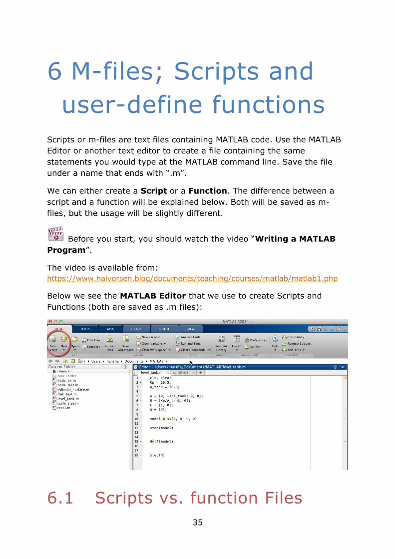
Below we see the MATLAB Editor that we use to create Scripts and
Functions (both are saved as .m files):
6.1 Scripts vs. function Files
36 M-files; Scripts and user-define
functions
MATLAB Course - Part I: Introduction to MATLAB
It is important to know the difference between a Script and a Function.
Scripts:
• A collection of commands that you would execute in the Command
Window
• Used for automating repetitive tasks
Functions:
• Operate on information (inputs) fed into them and return outputs
• Have a separate workspace and internal variables that is only valid
inside the function
• Your own user-defined functions work the same way as the built-in
functions you use all the time, such as plot(), rand(), mean(), std(),
etc.
MATLAB have lots of built-in functions, but very often we need to create
our own functions (these are called user-defined functions)
Below we will learn more about Scripts and Functions.
6.2 Scripts
A Script is a collection of MATLAB commands and functions that is bundled
together in a m-file. When you run the Script, all the commands are
executed sequentially.
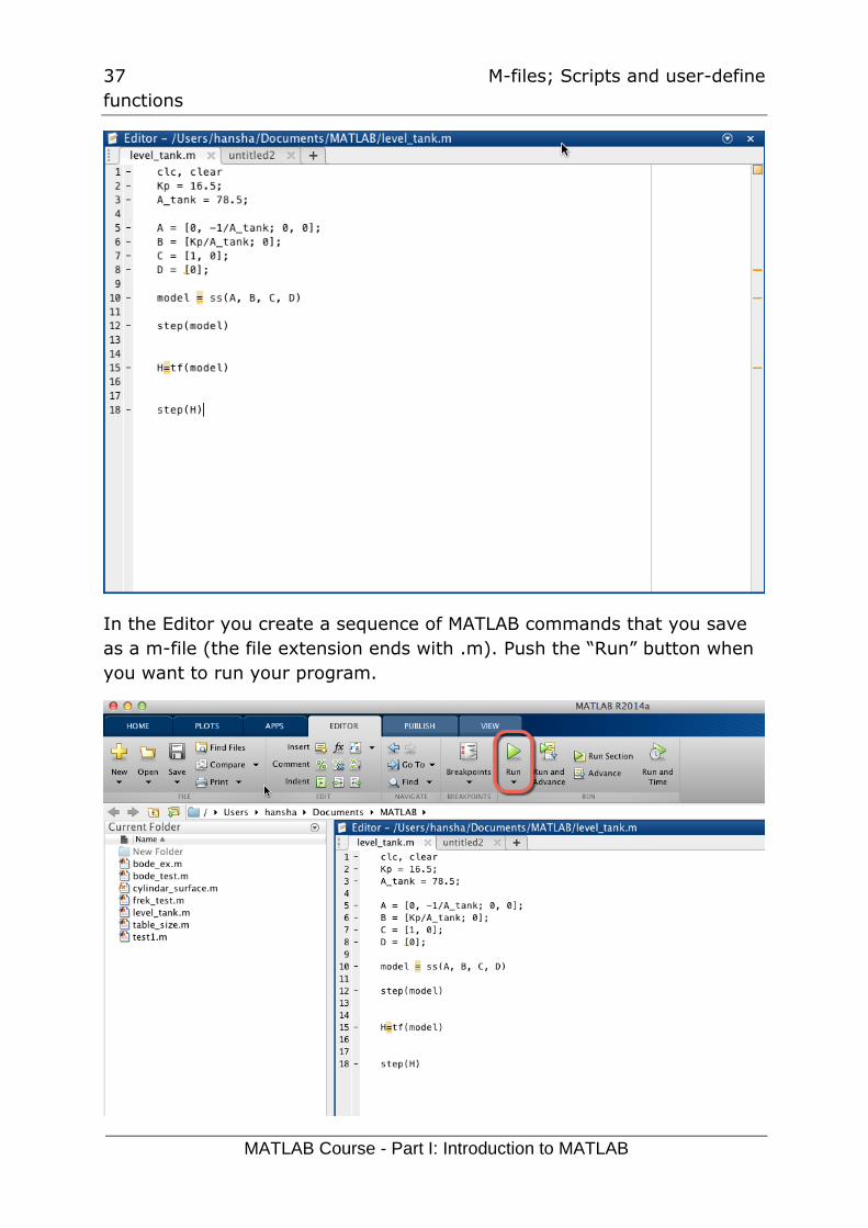
The built-in Editor for creating and modifying m-files are shown below:
37 M-files; Scripts and user-define
functions
MATLAB Course - Part I: Introduction to MATLAB
In the Editor you create a sequence of MATLAB commands that you save
as a m-file (the file extension ends with .m). Push the “Run” button when
you want to run your program.
38 M-files; Scripts and user-define
functions
MATLAB Course - Part I: Introduction to MATLAB
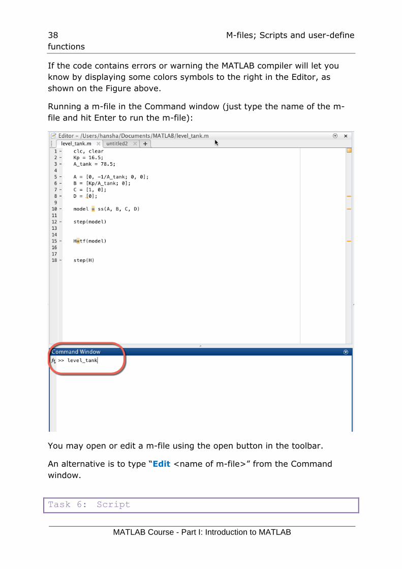
If the code contains errors or warning the MATLAB compiler will let you
know by displaying some colors symbols to the right in the Editor, as
shown on the Figure above.
Running a m-file in the Command window (just type the name of the m-
file and hit Enter to run the m-file):
You may open or edit a m-file using the open button in the toolbar.
An alternative is to type “Edit <name of m-file>” from the Command
window.
Task 6: Script
39 M-files; Scripts and user-define
functions
MATLAB Course - Part I: Introduction to MATLAB
Create a Script (M-file) where you create a vector with random data and
find the average and the standard deviation
Run the Script from the Command window.
[End of Task]
6.3 Functions
MATLAB includes more than 1000 built-in functions that you can use, but
sometimes you need to create your own functions.
To define your own function in MATLAB, use the following syntax:
function outputs = function_name(inputs)
% documentation
…
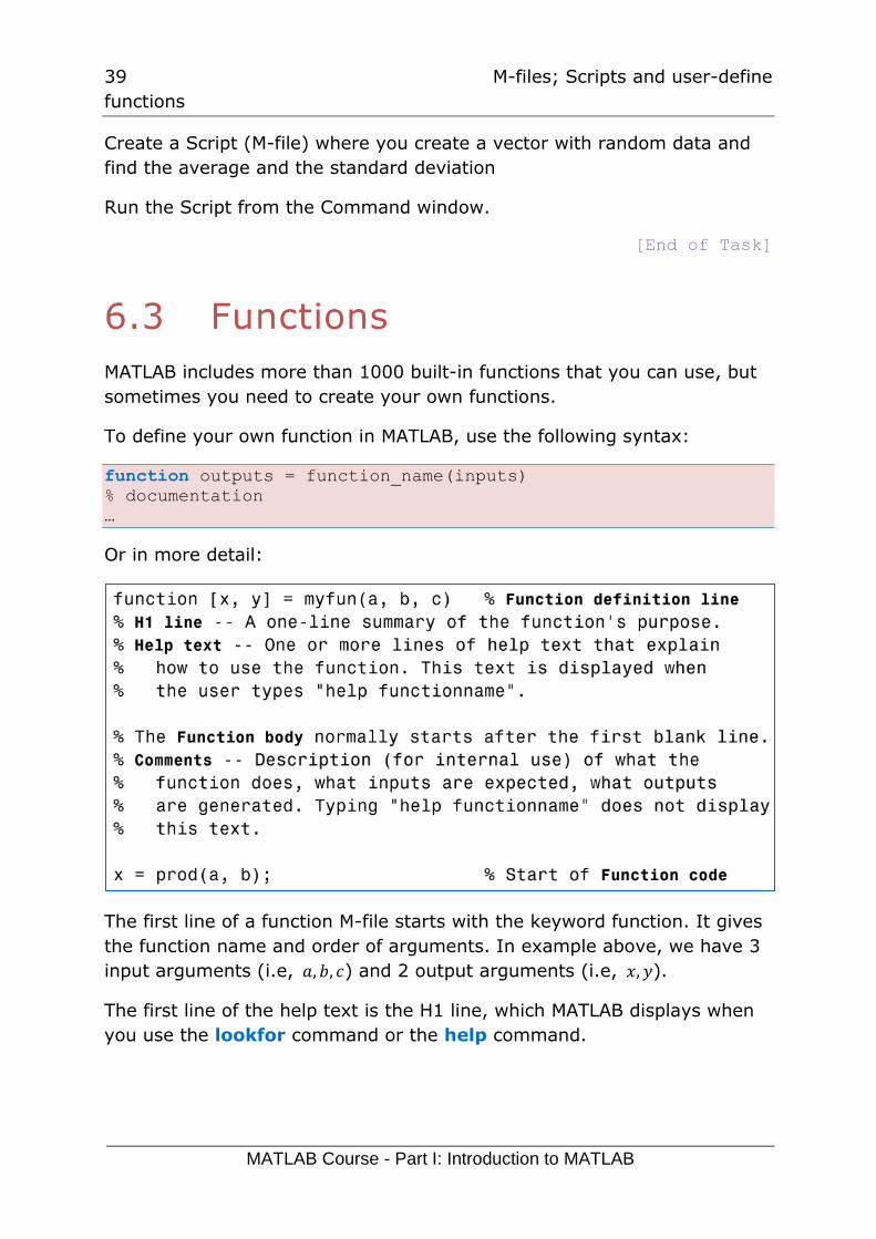
Or in more detail:
The first line of a function M-file starts with the keyword function. It gives
the function name and order of arguments. In example above, we have 3
input arguments (i.e, 𝑎, 𝑏, 𝑐) and 2 output arguments (i.e, 𝑥, 𝑦).
The first line of the help text is the H1 line, which MATLAB displays when
you use the lookfor command or the help command.
40 M-files; Scripts and user-define
functions
MATLAB Course - Part I: Introduction to MATLAB
Note! It is recommended that you use lowercase in the function name.
You should neither use spaces; use an underscore “_” if you need to
separate words.
A Function can have one or more inputs and one or more outputs.
Below we see how to declare a function with one input and one output:
Below we see how to declare a function with multiple inputs and multiple
outputs:
Example:
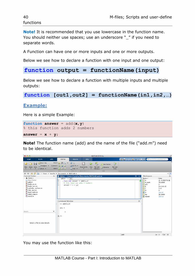
Here is a simple Example:
function answer = add(x,y)
% this function adds 2 numbers
answer = x + y;
Note! The function name (add) and the name of the file (“add.m”) need
to be identical.
You may use the function like this:
41 M-files; Scripts and user-define
functions
MATLAB Course - Part I: Introduction to MATLAB
% Example 1:
add(2,3)
% Example 2:
a = 4;
b = 6;
add(a,b);
% Example 3:
answer = add(a,b)
[End of Example]
You may create your own functions and save them as a m-file. Functions
are M-files that can accept input arguments and return output arguments.
Functions operate on variables within their own workspace, separate from
the workspace you access at the MATLAB command prompt.
Note! The name of the M-file and of the function should be the same!
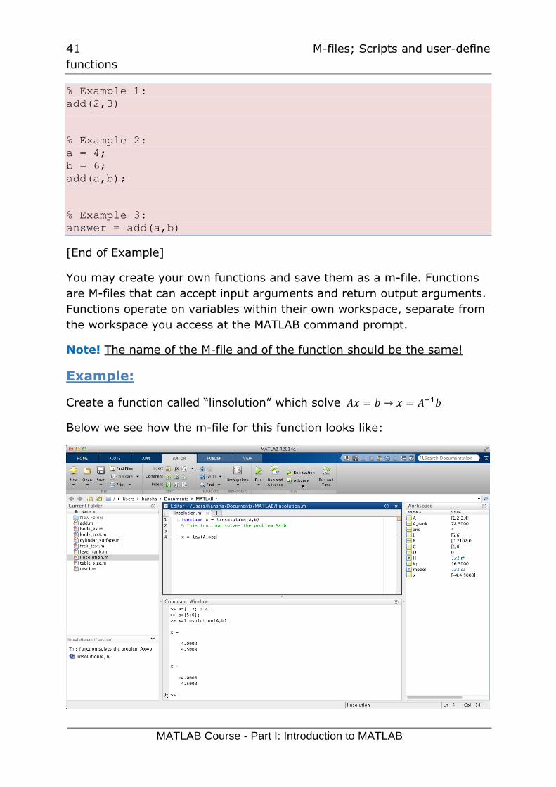
Example:
Create a function called “linsolution” which solve 𝐴𝑥 = 𝑏 → 𝑥 = 𝐴−1𝑏
Below we see how the m-file for this function looks like:
42 M-files; Scripts and user-define
functions
MATLAB Course - Part I: Introduction to MATLAB
You may define 𝐴 and 𝑏 in the Command window and the use the
function on order to find 𝑥:
>> A=[1 2;3 4];
>> b=[5;6];
>> x = linsolution(A,b)
x =
-4.0000
4.5000
After the function declaration (function [x] = linsolution(A,b)) in
the m.file, you may write a description of the function. This is done with the Comment sign “%” before each line.
From the Command window you can then type “help <function name>”
in order to read this information:
>> help linsolution
Solves the problem Ax=b using x=inv(A)*b
Created By Hans-Petter Halvorsen
[End of Example]
Naming a Function Uniquely:
To avoid choosing a name for a new function that might conflict with a
name already in use, check for any occurrences of the name using this
command:
which -all functionname
Task 7: User-defined function
Create a function calc_average that finds the average of two numbers.
Test the function afterwards as follows:
>>x = 2;
>>y = 4;
>>z = calc_average(x,y)
[End of Task]
Task 8: User-defined function
43 M-files; Scripts and user-define
functions
MATLAB Course - Part I: Introduction to MATLAB
Create a function circle that finds the area in a circle based on the input
parameter 𝑟 (radius).
Run and test the function in the Command window.
[End of Task]
44
7 Plotting
Plotting is a very important and powerful feature in MATLAB. In this
chapter we will learn the basic plotting functionality in MATLAB.
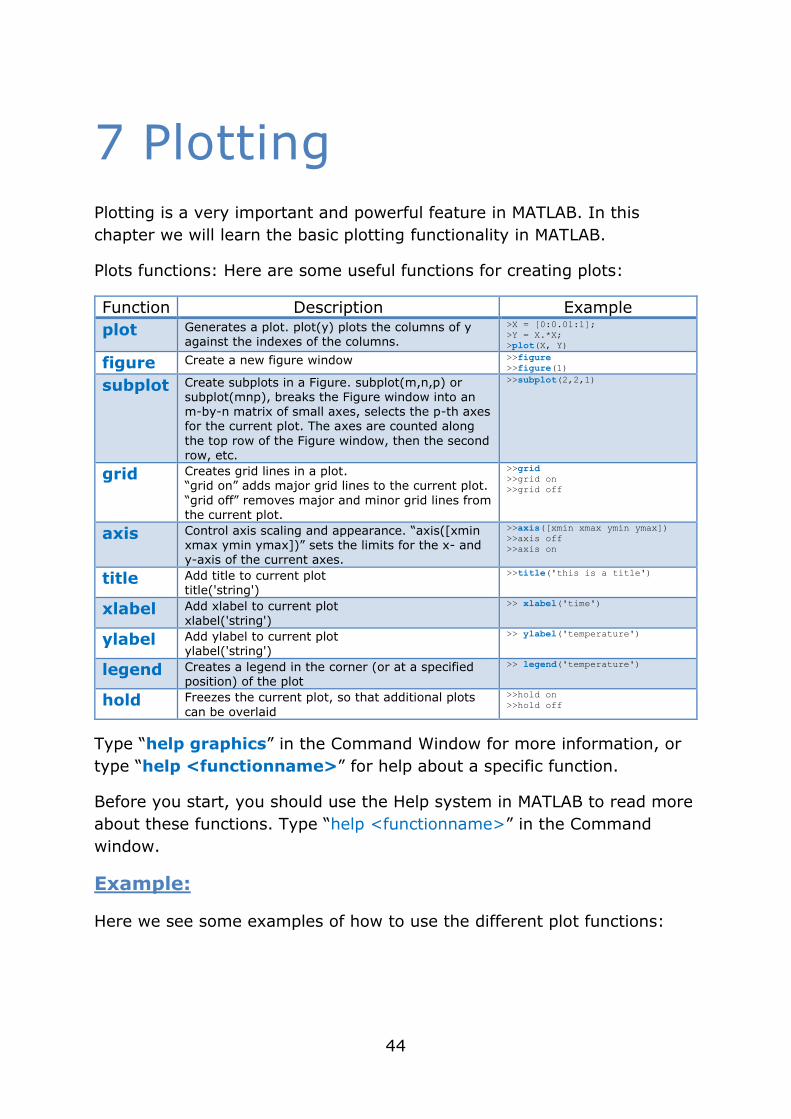
Plots functions: Here are some useful functions for creating plots:
Function Description Example
plot Generates a plot. plot(y) plots the columns of y against the indexes of the columns.
>X = [0:0.01:1];
>Y = X.*X;
>plot(X, Y)
figure Create a new figure window >>figure
>>figure(1)
subplot Create subplots in a Figure. subplot(m,n,p) or subplot(mnp), breaks the Figure window into an m-by-n matrix of small axes, selects the p-th axes for the current plot. The axes are counted along
the top row of the Figure window, then the second row, etc.
>>subplot(2,2,1)
grid Creates grid lines in a plot. “grid on” adds major grid lines to the current plot.
“grid off” removes major and minor grid lines from the current plot.
>>grid
>>grid on
>>grid off
axis Control axis scaling and appearance. “axis([xmin xmax ymin ymax])” sets the limits for the x- and y-axis of the current axes.
>>axis([xmin xmax ymin ymax])
>>axis off
>>axis on
title Add title to current plot title('string')
>>title('this is a title')
xlabel Add xlabel to current plot
xlabel('string')
>> xlabel('time')
ylabel Add ylabel to current plot ylabel('string')
>> ylabel('temperature')
legend Creates a legend in the corner (or at a specified position) of the plot
>> legend('temperature')
hold Freezes the current plot, so that additional plots
can be overlaid
>>hold on
>>hold off
Type “help graphics” in the Command Window for more information, or
type “help <functionname>” for help about a specific function.
Before you start, you should use the Help system in MATLAB to read more
about these functions. Type “help <functionname>” in the Command
window.
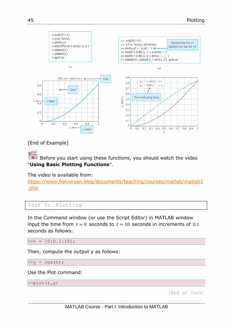
Example:
Here we see some examples of how to use the different plot functions:
45 Plotting
MATLAB Course - Part I: Introduction to MATLAB
[End of Example]
Before you start using these functions, you should watch the video
“Using Basic Plotting Functions”.
The video is available from:
https://www.halvorsen.blog/documents/teaching/courses/matlab/matlab1
.php
Task 9: Plotting
In the Command window (or use the Script Editor) in MATLAB window
input the time from 𝑡 = 0 seconds to 𝑡 = 10 seconds in increments of 0.1
seconds as follows:
>>t = [0:0.1:10];
Then, compute the output y as follows:
>>y = cos(t);
Use the Plot command:
>>plot(t,y)
[End of Task]
46 Plotting
MATLAB Course - Part I: Introduction to MATLAB
7.1 Plotting Multiple Data Sets in
One Graph
In MATLAB it is easy to plot multiple data set in one graph.
Example:
x = 0:pi/100:2*pi;
y = sin(x);
y2 = sin(x-.25);
y3 = sin(x-.5);
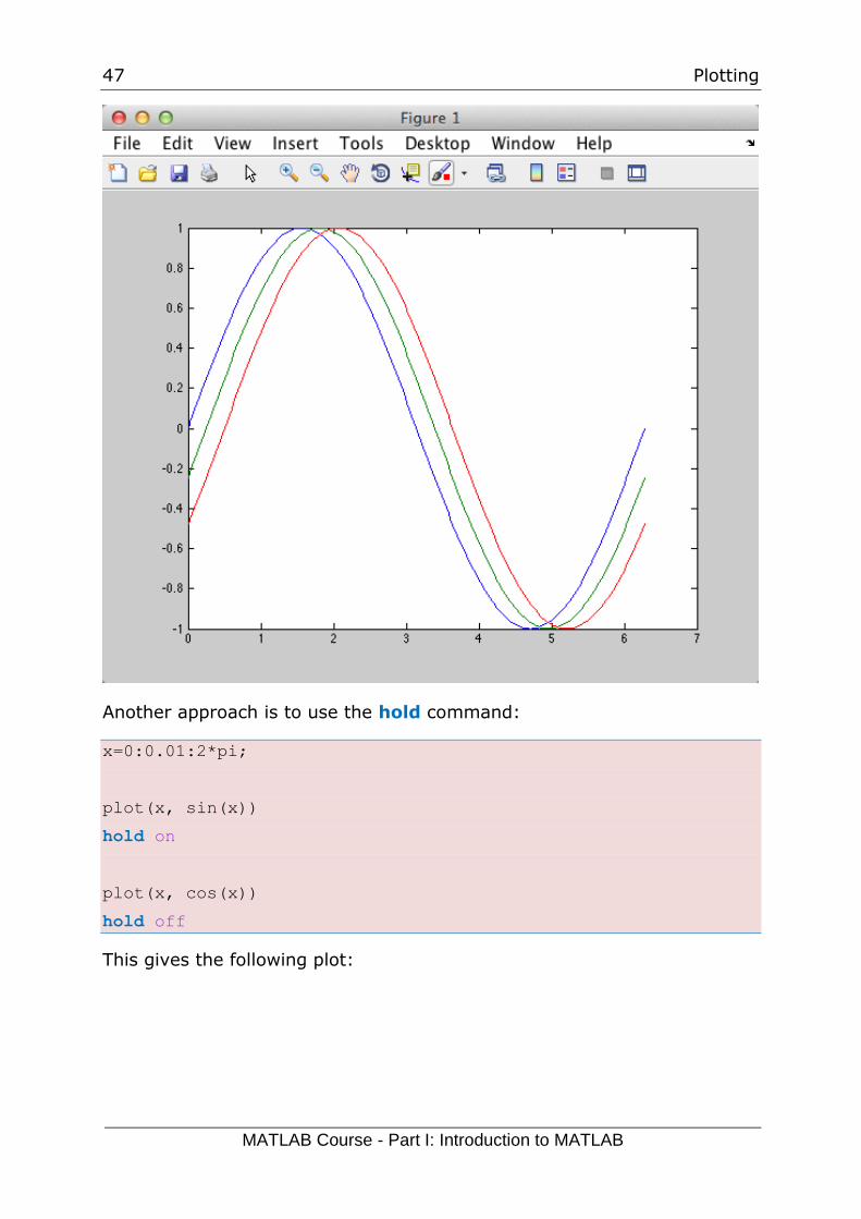
plot(x,y, x,y2, x,y3)
This gives the following plot:
47 Plotting
MATLAB Course - Part I: Introduction to MATLAB
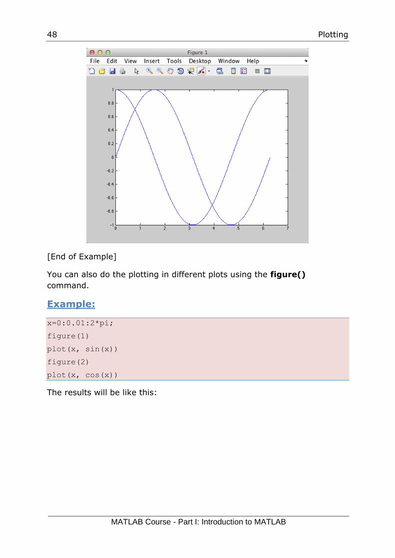
Another approach is to use the hold command:
x=0:0.01:2*pi;
plot(x, sin(x))
hold on
plot(x, cos(x))
hold off
This gives the following plot:
48 Plotting
MATLAB Course - Part I: Introduction to MATLAB
[End of Example]
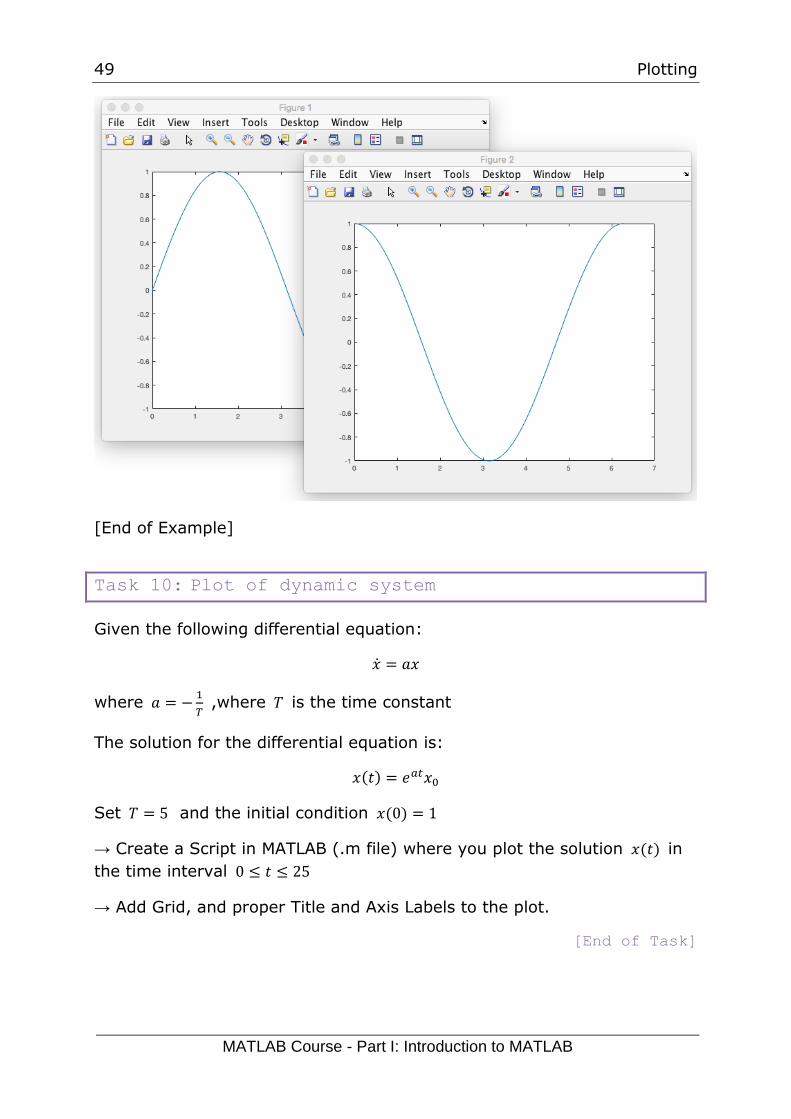
You can also do the plotting in different plots using the figure()
command.
Example:
x=0:0.01:2*pi;
figure(1)
plot(x, sin(x))
figure(2)
plot(x, cos(x))
The results will be like this:
49 Plotting
MATLAB Course - Part I: Introduction to MATLAB
[End of Example]
Task 10: Plot of dynamic system
Given the following differential equation:
�̇� = 𝑎𝑥
where 𝑎 = −1
𝑇 ,where 𝑇 is the time constant
The solution for the differential equation is:
𝑥(𝑡) = 𝑒𝑎𝑡𝑥0
Set 𝑇 = 5 and the initial condition 𝑥(0) = 1
→ Create a Script in MATLAB (.m file) where you plot the solution 𝑥(𝑡) in
the time interval 0 ≤ 𝑡 ≤ 25
→ Add Grid, and proper Title and Axis Labels to the plot.
[End of Task]
50 Plotting
MATLAB Course - Part I: Introduction to MATLAB
7.2 Displaying Multiple Plots in
one Figure – Sub-Plots
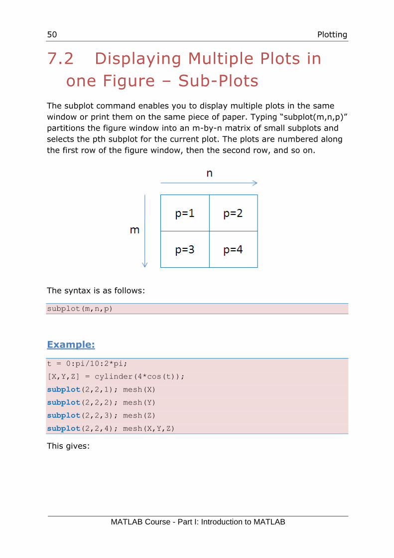
The subplot command enables you to display multiple plots in the same
window or print them on the same piece of paper. Typing “subplot(m,n,p)”
partitions the figure window into an m-by-n matrix of small subplots and
selects the pth subplot for the current plot. The plots are numbered along
the first row of the figure window, then the second row, and so on.
The syntax is as follows:
subplot(m,n,p)
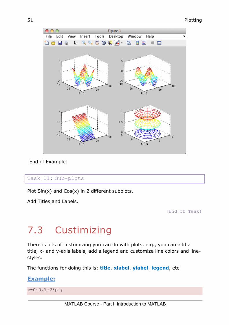
Example:
t = 0:pi/10:2*pi;
[X,Y,Z] = cylinder(4*cos(t));
subplot(2,2,1); mesh(X)
subplot(2,2,2); mesh(Y)
subplot(2,2,3); mesh(Z)
subplot(2,2,4); mesh(X,Y,Z)
This gives:
51 Plotting
MATLAB Course - Part I: Introduction to MATLAB
[End of Example]
Task 11: Sub-plots
Plot Sin(x) and Cos(x) in 2 different subplots.
Add Titles and Labels.
[End of Task]
7.3 Custimizing
There is lots of customizing you can do with plots, e.g., you can add a
title, x- and y-axis labels, add a legend and customize line colors and line-
styles.
The functions for doing this is; title, xlabel, ylabel, legend, etc.
Example:
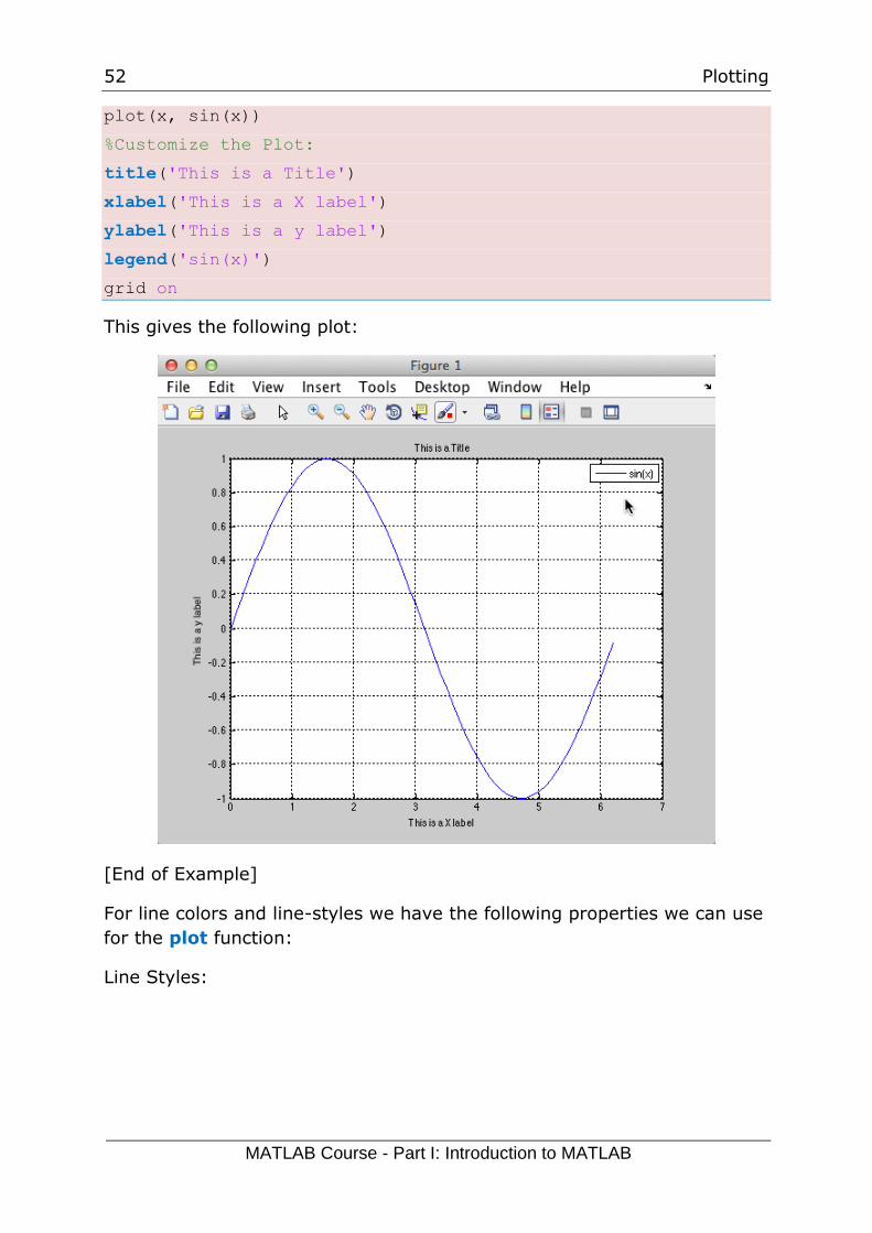
x=0:0.1:2*pi;
52 Plotting
MATLAB Course - Part I: Introduction to MATLAB
plot(x, sin(x))
%Customize the Plot:
title('This is a Title')
xlabel('This is a X label')
ylabel('This is a y label')
legend('sin(x)')
grid on
This gives the following plot:
[End of Example]
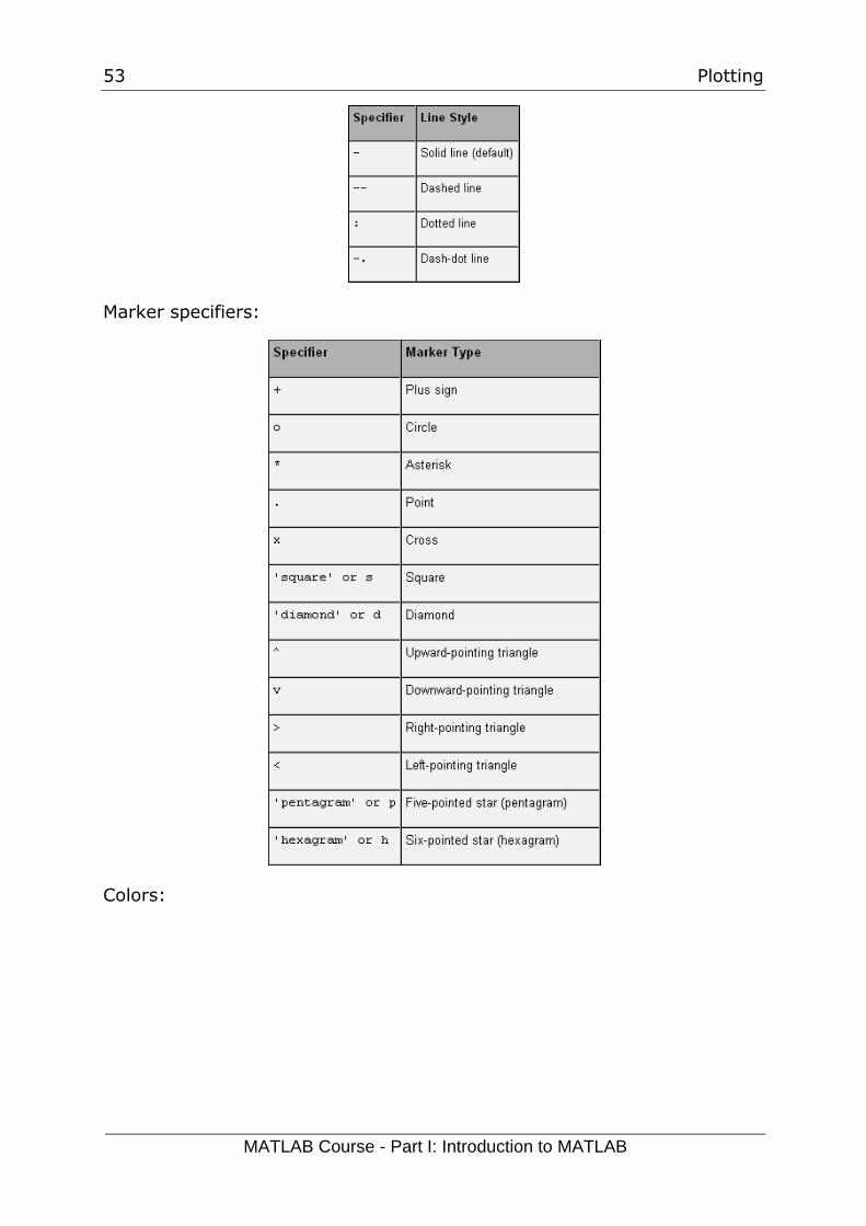
For line colors and line-styles we have the following properties we can use
for the plot function:
Line Styles:
53 Plotting
MATLAB Course - Part I: Introduction to MATLAB
Marker specifiers:
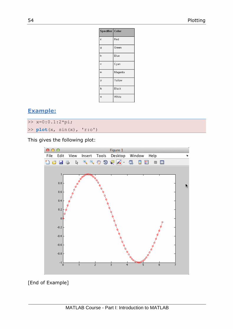
Colors:
54 Plotting
MATLAB Course - Part I: Introduction to MATLAB
Example:
>> x=0:0.1:2*pi;
>> plot(x, sin(x), 'r:o')
This gives the following plot:
[End of Example]
55 Plotting
MATLAB Course - Part I: Introduction to MATLAB
7.4 Other Plots
MATLAB offers lots of different plots.
Task 12: Other Plots
Check out the help for the following 2D functions in MATLAB: loglog,
semilogx, semilogy, plotyy, polar, fplot, fill, area, bar, barh, hist, pie,
errorbar, scatter.
→ Try some of them, e.g., bar, hist and pie.
[End of Task]
56
8 Flow Control and
Loops
8.1 Introduction
You may use different loops in MATLAB
• For loop
• While loop
If you want to control the flow in your program, you may want to use one
of the following:
• If-else statement
• Switch and case statement
It is assumed you know about For Loops, While Loops, If-Else and Switch
statements from other programming languages, so we will briefly show
the syntax used in MATLAB and go through some simple examples.
8.2 If-else Statement
The “if” statement evaluates a logical expression and executes a group of
statements when the expression is true. The optional “elseif” and else
keywords provide for the execution of alternate groups of statements. An
“end” keyword, which matches the “if”, terminates the last group of
statements. The groups of statements are delineated by the four
keywords—no braces or brackets are involved.
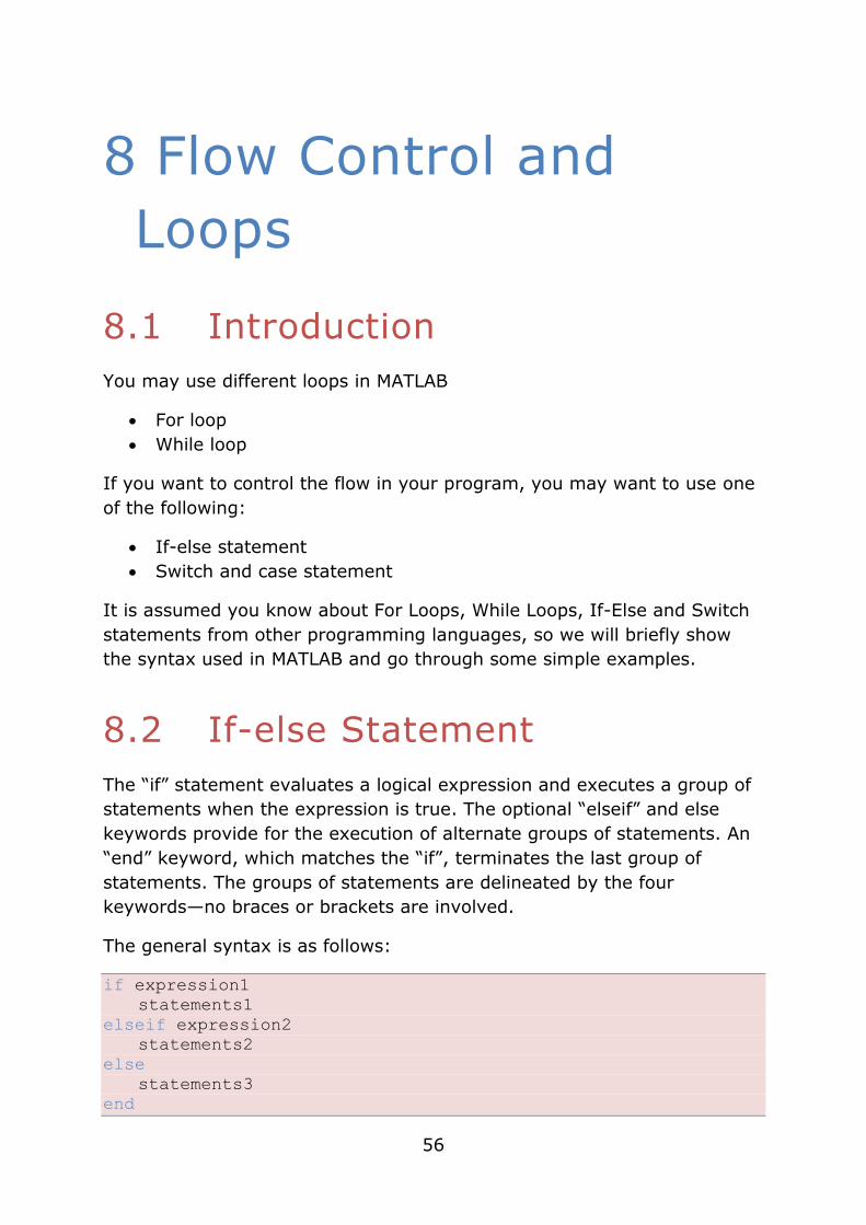
The general syntax is as follows:
if expression1
statements1
elseif expression2
statements2
else
statements3
end
57 Flow Control and Loops
MATLAB Course - Part I: Introduction to MATLAB
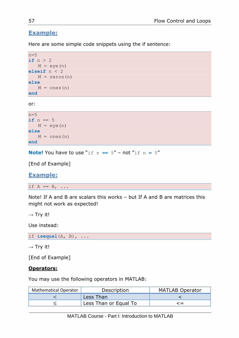
Example:
Here are some simple code snippets using the if sentence:
n=5
if n > 2
M = eye(n)
elseif n < 2
M = zeros(n)
else
M = ones(n)
end
or:
n=5
if n == 5
M = eye(n)
else
M = ones(n)
end
Note! You have to use “if n == 5” – not ”if n = 5”
[End of Example]
Example:
if A == B, ...
Note! If A and B are scalars this works – but If A and B are matrices this
might not work as expected!
→ Try it!
Use instead:
if isequal(A, B), ...
→ Try it!
[End of Example]
Operators:
You may use the following operators in MATLAB:
Mathematical Operator Description MATLAB Operator
< Less Than <
≤ Less Than or Equal To <=
58 Flow Control and Loops
MATLAB Course - Part I: Introduction to MATLAB
> Greater Than >
≥ Greater Than or Equal To >=
= Equal To ==
≠ Not Equal To ~=
Logical Operators:
You may use the following logical operators in MATLAB:
Logical Operator MATLAB Operator
AND &
OR |
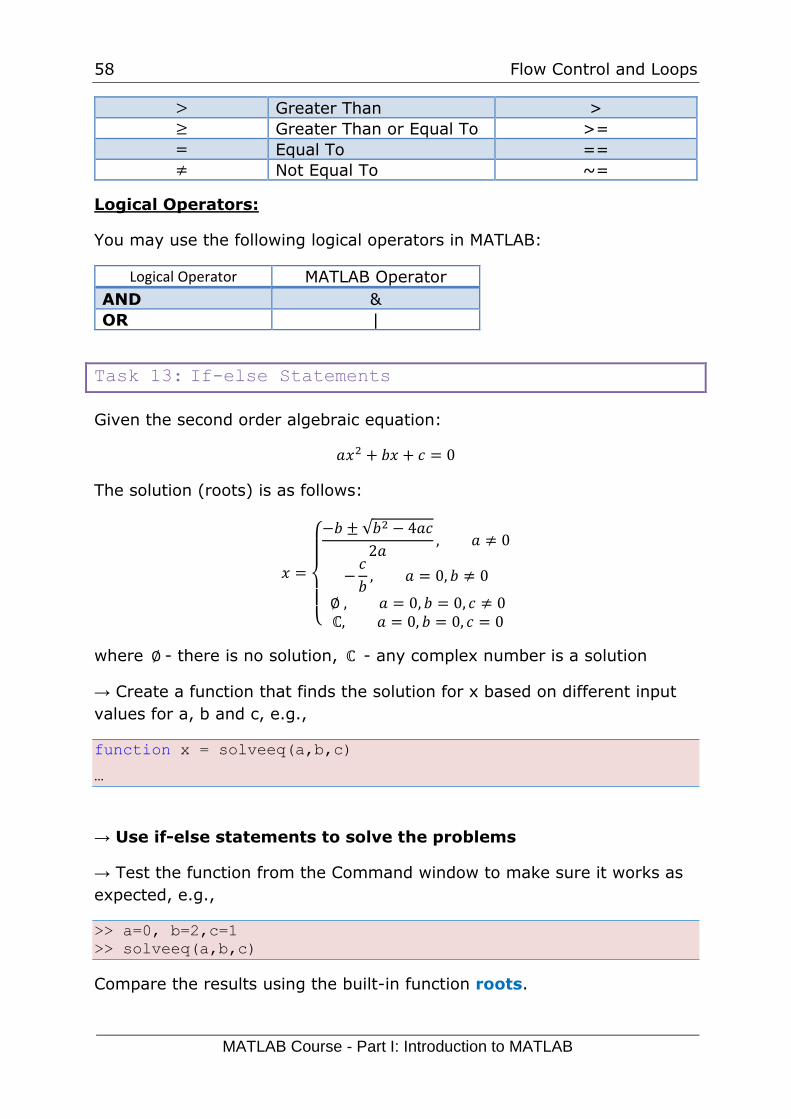
Task 13: If-else Statements
Given the second order algebraic equation:
𝑎𝑥2 + 𝑏𝑥 + 𝑐 = 0
The solution (roots) is as follows:
𝑥 =
{
−𝑏 ± √𝑏
2 − 4𝑎𝑐
2𝑎, 𝑎 ≠ 0
−𝑐
𝑏, 𝑎 = 0, 𝑏 ≠ 0
∅ , 𝑎 = 0, 𝑏 = 0, 𝑐 ≠ 0ℂ, 𝑎 = 0, 𝑏 = 0, 𝑐 = 0
where ∅ - there is no solution, ℂ - any complex number is a solution
→ Create a function that finds the solution for x based on different input
values for a, b and c, e.g.,
function x = solveeq(a,b,c)
…
→ Use if-else statements to solve the problems
→ Test the function from the Command window to make sure it works as
expected, e.g.,
>> a=0, b=2,c=1
>> solveeq(a,b,c)
Compare the results using the built-in function roots.
59 Flow Control and Loops
MATLAB Course - Part I: Introduction to MATLAB
Tip! For ∅, you can just type disp(‘there is no solution’) and for ℂ you can
type disp(‘any complex number is a solution’) – or something like that.
[End of Task]
8.3 Switch and Case Statement
The switch statement executes groups of statements based on the value
of a variable or expression. The keywords case and otherwise delineate
the groups. Only the first matching case is executed. There must always
be an end to match the switch.
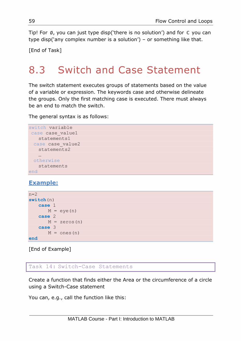
The general syntax is as follows:
switch variable
case case_value1
statements1
case case_value2
statements2
…
otherwise
statements
end
Example:
n=2
switch(n)
case 1
M = eye(n)
case 2
M = zeros(n)
case 3
M = ones(n)
end
[End of Example]
Task 14: Switch-Case Statements
Create a function that finds either the Area or the circumference of a circle
using a Switch-Case statement
You can, e.g., call the function like this:
60 Flow Control and Loops
MATLAB Course - Part I: Introduction to MATLAB
>> r=2;
>> calccircl(r,1) % 1 means area
>> calccircl(r,2) % 2 means circumference
[End of Task]
8.4 For loop
The For loop repeats a group of statements a fixed, predetermined
number of times. A matching end delineates the statements.
The general syntax is as follows:
for variable = initval:endval
statement
...
statement
end
Example:
m=5
for n = 1:m
r(n) = rank(magic(n));
end
r
[End of Example]
Task 15: Fibonacci Numbers
In mathematics, Fibonacci numbers are the numbers in the following
sequence:
0, 1, 1, 2 ,3, 5, 8, 13, 21, 34, 55, 89, 144, …
By definition, the first two Fibonacci numbers are 0 and 1, and each
subsequent number is the sum of the previous two. Some sources omit
the initial 0, instead beginning the sequence with two 1s.
In mathematical terms, the sequence Fn of Fibonacci numbers is defined
by the recurrence relation:
61 Flow Control and Loops
MATLAB Course - Part I: Introduction to MATLAB
𝑓𝑛 = 𝑓𝑛−1 + 𝑓𝑛−2
with seed values:
𝑓0 = 0, 𝑓1 = 1
→ Write a function in MATLAB that calculates the N first Fibonacci
numbers, e.g.,
>> N=10;
>> fibonacci(N)
ans =
0
1
1
2
3
5
8
13
21
34
→ Use a For loop to solve the problem.
Fibonacci numbers are used in the analysis of financial markets, in
strategies such as Fibonacci retracement, and are used in computer
algorithms such as the Fibonacci search technique and the Fibonacci heap
data structure. They also appear in biological settings, such as branching
in trees, arrangement of leaves on a stem, the fruitlets of a pineapple, the
flowering of artichoke, an uncurling fern and the arrangement of a pine
cone.
[End of Task]
8.5 While loop
The while loop repeats a group of statements an indefinite number of
times under control of a logical condition. A matching end delineates the
statements.
The general syntax is as follows:
while expression
62 Flow Control and Loops
MATLAB Course - Part I: Introduction to MATLAB
statements
end
Example:
m=5;
while m > 1
m = m - 1;
zeros(m)
end
[End of Example]
Task 16: While Loop
Create a Script or Function that creates Fibonacci Numbers up to a given
number, e.g.,
>> maxnumber=2000;
>> fibonacci(maxnumber)
Use a While Loop to solve the problem.
[End of Task]
8.6 Additional Tasks
Here are some additional tasks about Loops and Flow control.
Task 17: For Loops
Extend your calc_average function from a previous task so it can
calculate the average of a vector with random elements. Use a For loop to
iterate through the values in the vector and find sum in each iteration:
mysum = mysum + x(i);
Test the function in the Command window
[End of Task]
63 Flow Control and Loops
MATLAB Course - Part I: Introduction to MATLAB
Task 18: If-else Statement
Create a function where you use the “if-else” statement to find elements
larger than a specific value in the task above. If this is the case, discard
these values from the calculated average.
Example discarding numbers larger than 10 gives:
x =
4 6 12
>> calc_average(x)
ans =
5
[End of Task]
64
9 Mathematics
MATLAB is a powerful tool for mathematical calculations.
Type “help elfun” (elementary functions) in the Command window for
more information about basic mathematical functions.
9.1 Basic Math Functions
Some Basic Math functions in MATLAB: exp, sqrt, log, etc.→ Look up
these functions in the Help system in MATLAB.
Task 19: Basic Math function
Create a function that calculates the following mathematical expression:
𝑧 = 3𝑥2 + √𝑥2 + 𝑦2 + 𝑒ln (𝑥)
Test with different values for 𝑥 and 𝑦.
[End of Task]
9.2 Statistics
Some Statistics functions in MATLAB: mean, max, min, std, etc.
→ Look up these functions in the Help system in MATLAB.
Task 20: Statistics
Create a vector with random numbers between 0 and 100. Find the
following statistics: mean, median, standard deviation, minimum,
maximum and the variance.
[End of Task]
65 Mathematics
MATLAB Course - Part I: Introduction to MATLAB
9.3 Trigonometric Functions
MATLAB offers lots of Trigonometric functions, e.g., sin, cos, tan, etc. →
Look up these functions in the Help system in MATLAB.
Note! Most of the trigonometric functions require that the angle is
expressed in radians.
Example:
>> sin(pi/4)
ans =
0.7071
[End of Example]
Task 21: Conversion
Since most of the trigonometric functions require that the angle is
expressed in radians, we will create our own functions in order to convert
between radians and degrees.
It is quite easy to convert from radians to degrees or from degrees to
radians. We have that:
2𝜋 [𝑟𝑎𝑑𝑖𝑎𝑛𝑠] = 360 [𝑑𝑒𝑔𝑟𝑒𝑒𝑠]
This gives:
𝑑 [𝑑𝑒𝑔𝑟𝑒𝑒𝑠] = 𝑟[𝑟𝑎𝑑𝑖𝑎𝑛𝑠] ∙ (180
𝜋)
𝑟[𝑟𝑎𝑑𝑖𝑎𝑛𝑠] = 𝑑[𝑑𝑒𝑔𝑟𝑒𝑒𝑠] ∙ (𝜋
180)
→ Create two functions that convert from radians to degrees (r2d(x))
and from degrees to radians (d2r(x)) respectively.
Test the functions to make sure that they work as expected.
[End of Task]
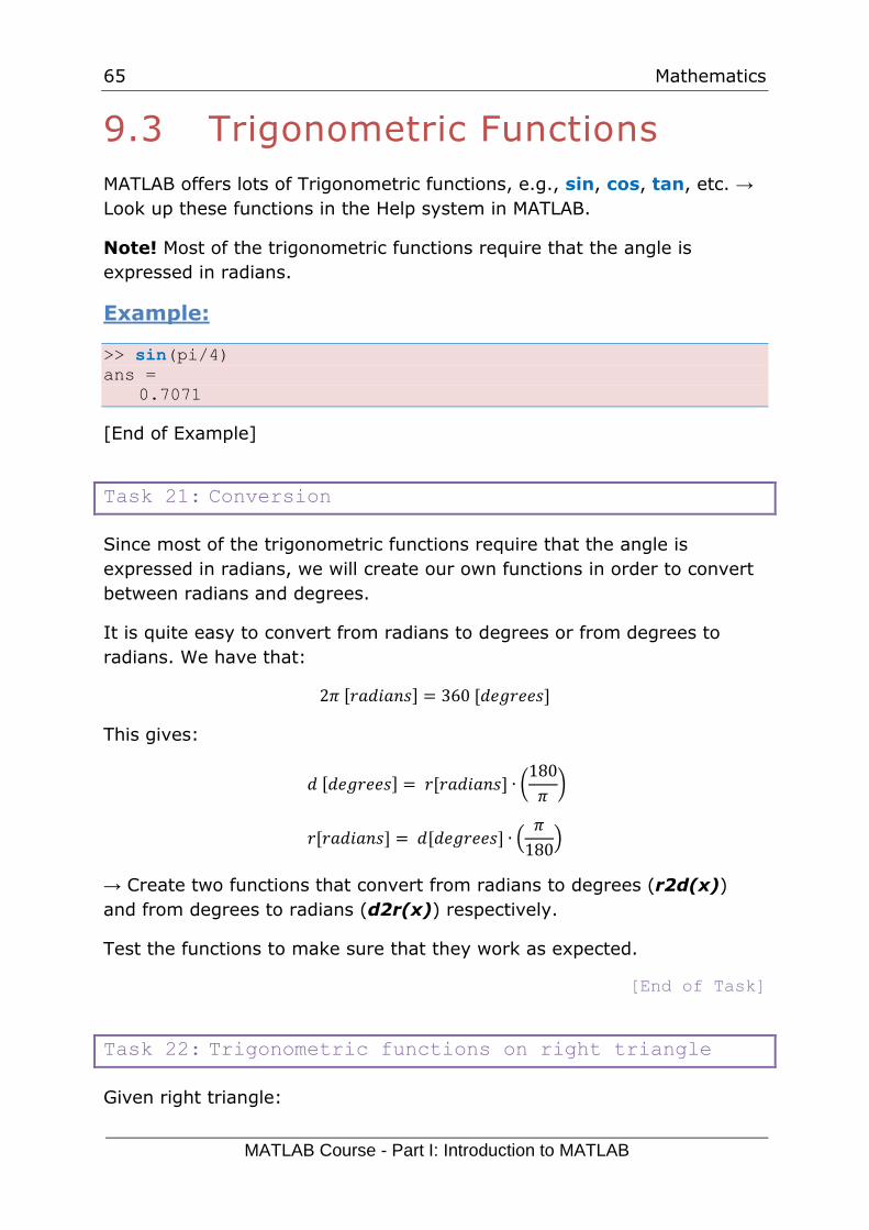
Task 22: Trigonometric functions on right triangle
Given right triangle:
66 Mathematics
MATLAB Course - Part I: Introduction to MATLAB
→ Create a function that finds the angle 𝐴 (in degrees) based on input
arguments (𝑎, 𝑐), (𝑏, 𝑐) and (𝑎, 𝑏) respectively.
Use, e.g., a third input “type” to define the different types above.
→ Use you previous function r2d() to make sure the output of your
function is in degrees and not in radians.
Test the functions to make sure it works properly.
Tip! We have that:
sin 𝐴 =𝑎
𝑐, 𝐴 = 𝑎𝑟𝑐𝑠𝑖𝑛 (
𝑎
𝑐)
cos 𝐴 =𝑏
𝑐, 𝐴 = 𝑎𝑟𝑐𝑐𝑜𝑠 (
𝑏
𝑐)
tan𝐴 =𝑎
𝑏, 𝐴 = 𝑎𝑟𝑐𝑡𝑎𝑛 (
𝑎
𝑏)
We may also need the Pythagoras' theorem:
𝑐2 = 𝑎2 + 𝑏2
Testing the function can be done like this in the Command Window:
>> a=5, b=8, c=sqrt(a^2+b^2);
>> A = right_triangle(a,c,'sin')
A =
32.0054
>> A = right_triangle(b,c,'cos')
A =
32.0054
>> A = right_triangle(a,b,'tan')
A =
67 Mathematics
MATLAB Course - Part I: Introduction to MATLAB
32.0054
We also see that the answer in this case is the same, which is expected.
[End of Task]
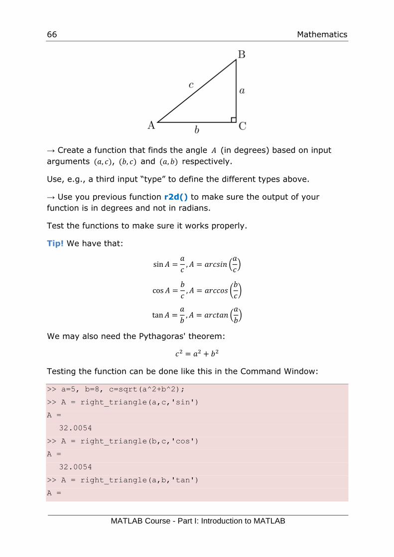
Task 23: Law of cosines
Given:
Create a function where you find c using the law of cosines.
𝑐2 = 𝑎2 + 𝑏2 − 2𝑎𝑏 𝑐𝑜𝑠𝐶
Test the functions to make sure it works properly.
[End of Task]
Task 24: Plotting
Plot 𝑠𝑖𝑛(𝜃) and 𝑐𝑜𝑠(𝜃) for 0 ≤ 𝜃 ≤ 2𝜋 in the same plot.
Make sure to add labels and a legend and use different line styles and
colors for the plots.
[End of Task]
9.4 Complex Numbers
Complex numbers are important in modelling and control theory.
A complex number is defined like this:
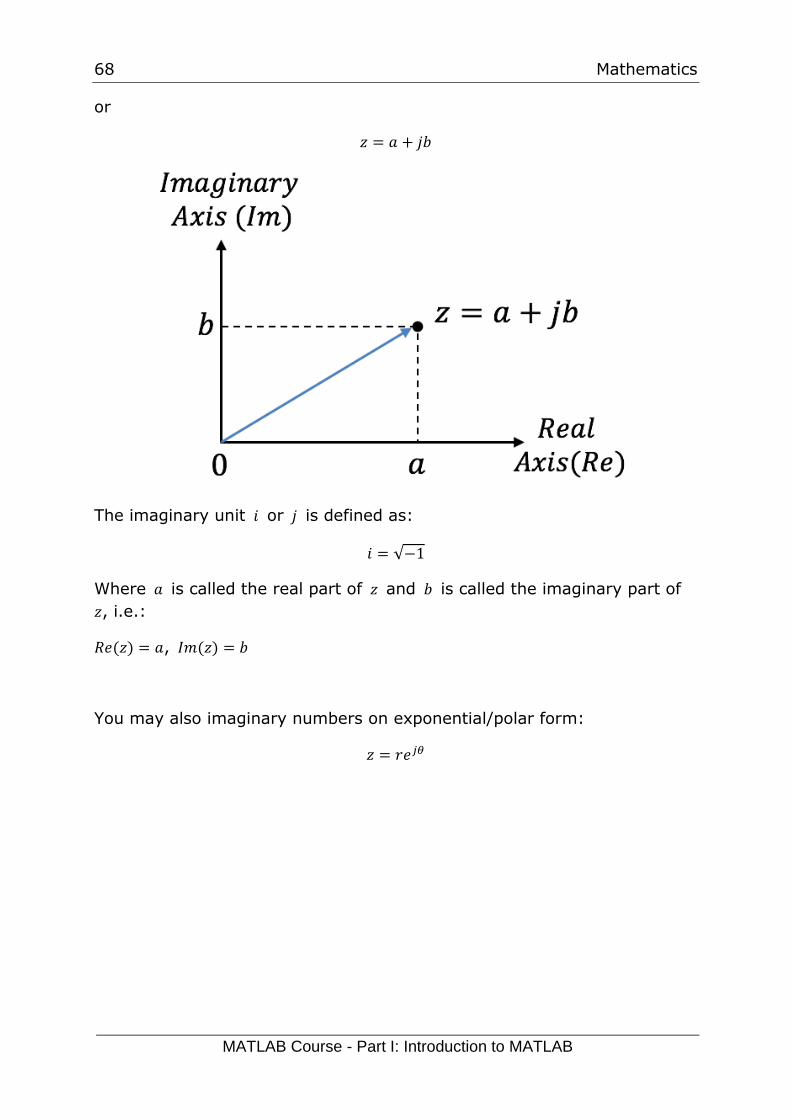
𝑧 = 𝑎 + 𝑖𝑏
68 Mathematics
MATLAB Course - Part I: Introduction to MATLAB
or
𝑧 = 𝑎 + 𝑗𝑏
The imaginary unit 𝑖 or 𝑗 is defined as:
𝑖 = √−1
Where 𝑎 is called the real part of 𝑧 and 𝑏 is called the imaginary part of
𝑧, i.e.:
𝑅𝑒(𝑧) = 𝑎, 𝐼𝑚(𝑧) = 𝑏
You may also imaginary numbers on exponential/polar form:
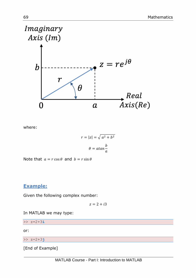
𝑧 = 𝑟𝑒𝑗𝜃
69 Mathematics
MATLAB Course - Part I: Introduction to MATLAB
where:
𝑟 = |𝑧| = √ 𝑎2 + 𝑏2
𝜃 = 𝑎𝑡𝑎𝑛𝑏
𝑎
Note that 𝑎 = 𝑟 cos 𝜃 and 𝑏 = 𝑟 sin 𝜃
Example:
Given the following complex number:
𝑧 = 2 + 𝑖3
In MATLAB we may type:
>> z=2+3i
or:
>> z=2+3j
[End of Example]
70 Mathematics
MATLAB Course - Part I: Introduction to MATLAB
The complex conjugate of z is defined as:
𝑧∗ = 𝑎 − 𝑖𝑏
To add or subtract two complex numbers, we simply add (or subtract)
their real parts and their imaginary parts.
In Division and multiplication, we use the polar form.
Given the complex numbers:
𝑧1 = 𝑟1𝑒𝑗𝜃1 and 𝑧2 = 𝑟2𝑒
𝑗𝜃2
Multiplication:
𝑧3 = 𝑧1𝑧2 = 𝑟1𝑟2𝑒𝑗(𝜃1+𝜃2)
Division:
𝑧3 =𝑧1𝑧2=𝑟1𝑒
𝑗𝜃1
𝑟2𝑒𝑗𝜃2
=𝑟1𝑟2𝑒𝑗(𝜃1−𝜃2)
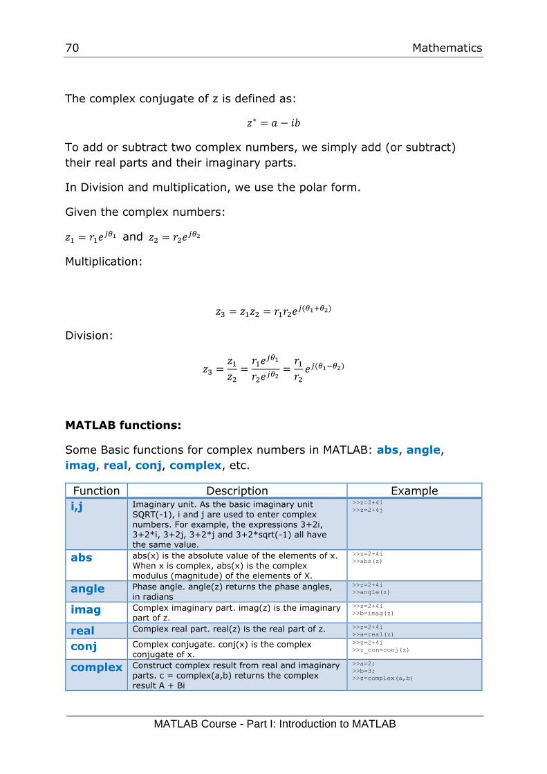
MATLAB functions:
Some Basic functions for complex numbers in MATLAB: abs, angle,
imag, real, conj, complex, etc.
Function Description Example
i,j Imaginary unit. As the basic imaginary unit
SQRT(-1), i and j are used to enter complex numbers. For example, the expressions 3+2i, 3+2*i, 3+2j, 3+2*j and 3+2*sqrt(-1) all have the same value.
>>z=2+4i
>>z=2+4j
abs abs(x) is the absolute value of the elements of x. When x is complex, abs(x) is the complex modulus (magnitude) of the elements of X.
>>z=2+4i
>>abs(z)
angle Phase angle. angle(z) returns the phase angles, in radians
>>z=2+4i
>>angle(z)
imag Complex imaginary part. imag(z) is the imaginary part of z.
>>z=2+4i
>>b=imag(z)
real Complex real part. real(z) is the real part of z. >>z=2+4i
>>a=real(z)
conj Complex conjugate. conj(x) is the complex conjugate of x.
>>z=2+4i
>>z_con=conj(z)
complex Construct complex result from real and imaginary parts. c = complex(a,b) returns the complex result A + Bi
>>a=2;
>>b=3;
>>z=complex(a,b)
71 Mathematics
MATLAB Course - Part I: Introduction to MATLAB
Look up these functions in the Help system in MATLAB.
Task 25: Complex numbers
Given two complex numbers
𝑐 = 4 + 𝑗3, 𝑑 = 1 − 𝑗
Find the real and imaginary part of c and d in MATLAB.
→ Use MATLAB to find 𝑐 + 𝑑, 𝑐 − 𝑑, 𝑐𝑑 𝑎𝑛𝑑 𝑐/𝑑.
Use the direct method supported by MATLAB and the specific complex
functions abs, angle, imag, real, conj, complex, etc. together with the
formulas for complex numbers that are listed above in the text (as you do
it when you should calculate it using pen & paper).
→ Find also 𝑟 and 𝜃. Find also the complex conjugate.
[End of Task]
Task 26: Complex numbers
Find the roots of the equation:
𝑥2 + 4𝑥 + 13
We can e.g., use the solveeq function we created in a previous task.
Compare the results using the built-in function roots.
Discuss the results.
Add the sum of the roots.
[End of Task]
9.5 Polynomials
A polynomial is expressed as:
𝑝(𝑥) = 𝑝1𝑥𝑛 + 𝑝2𝑥
𝑛−1 +⋯+ 𝑝𝑛𝑥 + 𝑝𝑛+1
where 𝑝1, 𝑝2, 𝑝3, … are the coefficients of the polynomial.
72 Mathematics
MATLAB Course - Part I: Introduction to MATLAB
MATLAB represents polynomials as row arrays containing coefficients
ordered by descending powers.
Example:
Given the polynomial:
𝑝(𝑥) = −5.45𝑥4 + 3.2𝑥2 + 8𝑥 + 5.6
In MATLAB we write:
>> p=[-5.45 0 3.2 8 5.8]
p =
-5.4500 0 3.2000 8.0000 5.8000
[End of Example]
MATLAB offers lots of functions on polynomials, such as conv, roots,
deconv, polyval, polyint, polyder, polyfit, etc. → Look up these
functions in the Help system in MATLAB.
Task 27: Polynomials
Define the following polynomial in MATLAB:
𝑝(𝑥) = −2.1𝑥4 + 2𝑥3 + 5𝑥 + 11
→ Find the roots of the polynomial (𝑝(𝑥) = 0) (and check if the answers are
correct)
→ Find 𝑝(𝑥 = 2)
Use the polynomial functions listed above.
[End of Task]
Task 28: Polynomials
Given the following polynomials:
𝑝1(𝑥) = 1 + 𝑥 − 𝑥2
𝑝2(𝑥) = 2 + 𝑥3
→ Find the polynomial 𝑝(𝑥) = 𝑝1(𝑥) ∙ 𝑝2(𝑥) using MATLAB and find the roots
→ Find the roots of the polynomial (𝑝(𝑥) = 0)
73 Mathematics
MATLAB Course - Part I: Introduction to MATLAB
→ Find 𝑝(𝑥 = 2)
→ Find the differentiation/derivative of 𝑝2(𝑥), i.e., 𝑝2′
Use the polynomial functions listed above.
[End of Task]
Task 29: Polynomial Fitting
Find the 6. order Polynomial that best fits the following function:
𝑦 = sin (𝑥)
Use the polynomial functions listed above.
→ Plot both the function and the 6. order Polynomial to compare the
results.
[End of Task]
74
10 Additional Tasks
If you have time left or need more practice, solve the tasks below. Its
highly recommended to solve these tasks as well, since some of these will
most likely be part of the final test.
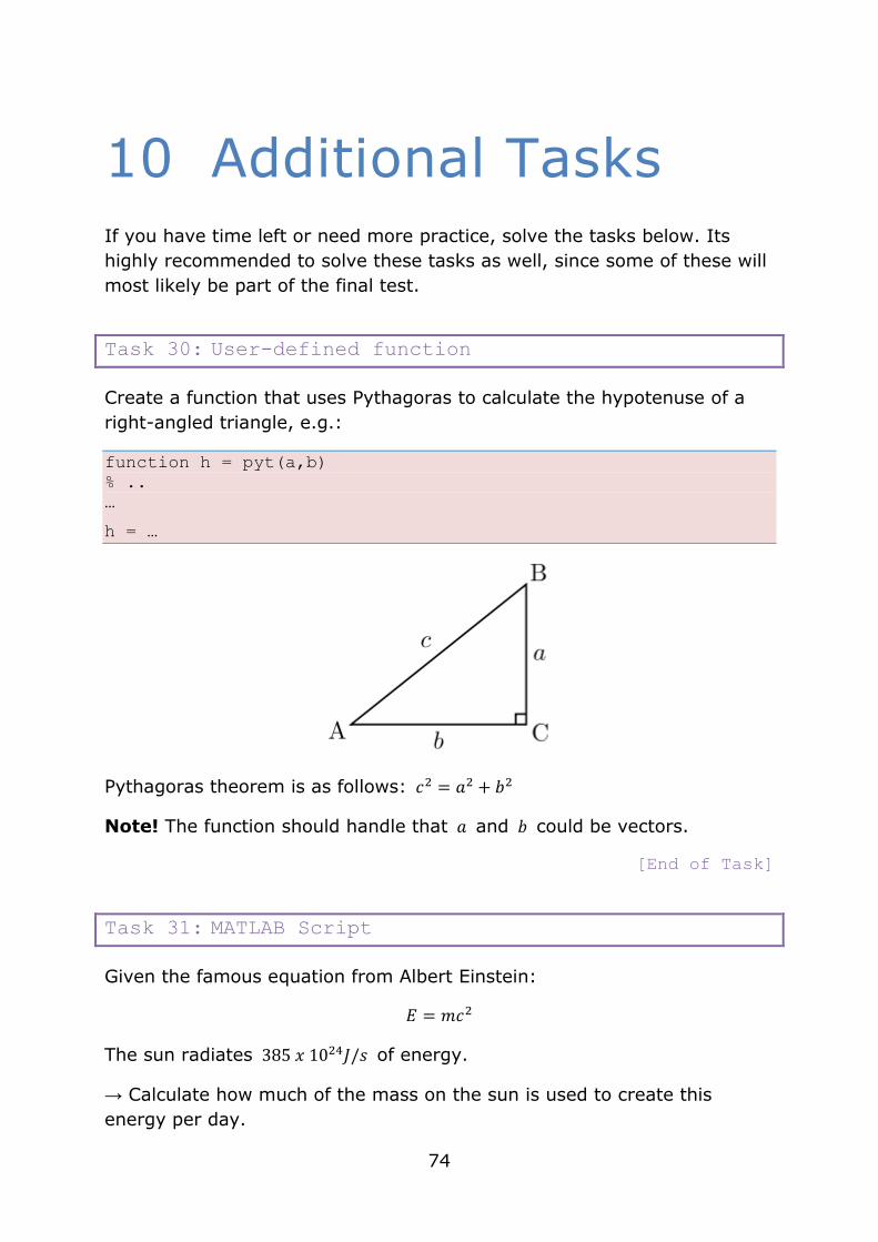
Task 30: User-defined function
Create a function that uses Pythagoras to calculate the hypotenuse of a
right-angled triangle, e.g.:
function h = pyt(a,b)
% ..
…
h = …
Pythagoras theorem is as follows: 𝑐2 = 𝑎2 + 𝑏2
Note! The function should handle that 𝑎 and 𝑏 could be vectors.
[End of Task]
Task 31: MATLAB Script
Given the famous equation from Albert Einstein:
𝐸 = 𝑚𝑐2
The sun radiates 385 𝑥 1024𝐽/𝑠 of energy.
→ Calculate how much of the mass on the sun is used to create this
energy per day.
75 Additional Tasks
MATLAB Course - Part I: Introduction to MATLAB
→ How many years will it take to convert all the mass of the sun
completely? Do we need to worry if the sun will be used up in our
generation or the next?
The mass of the sun is 2 𝑥 1030𝑘𝑔
[End of Task]
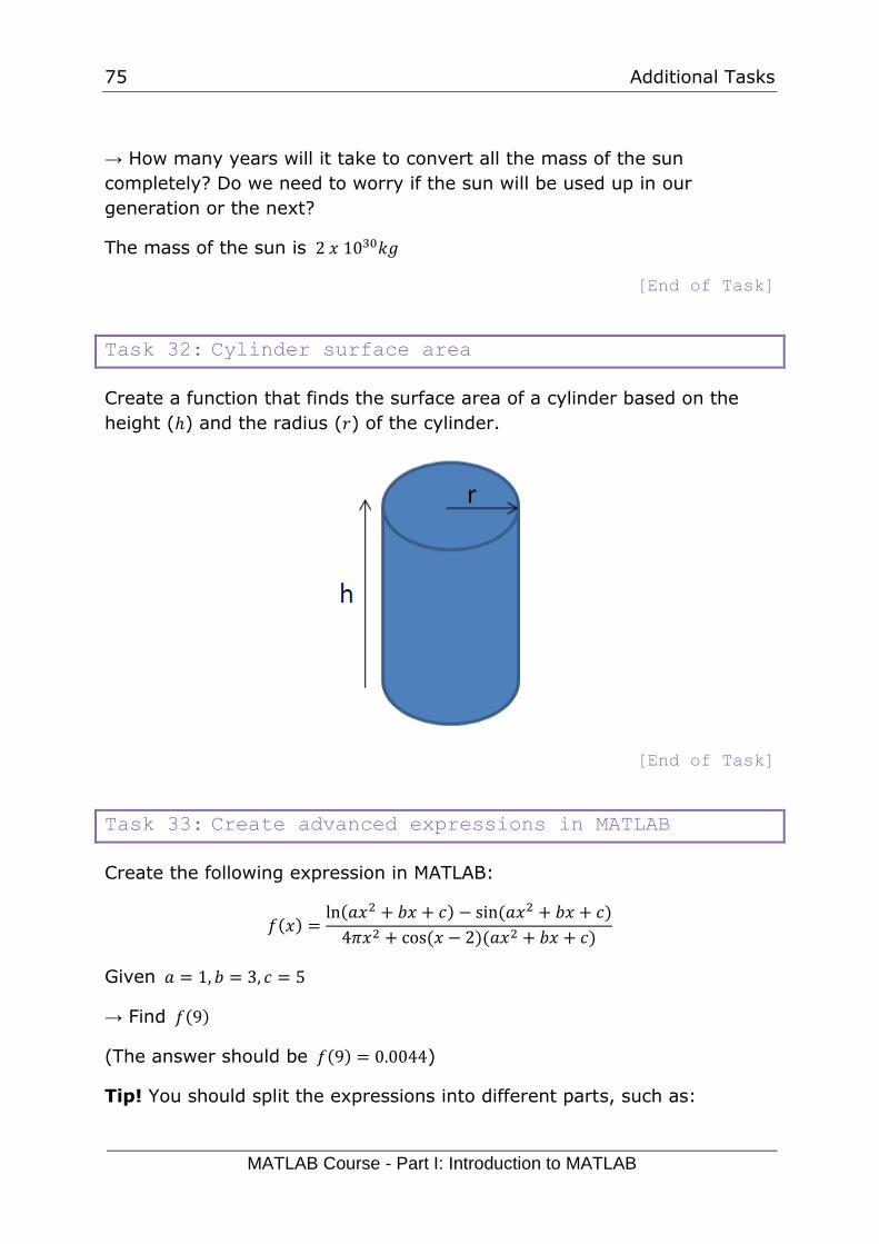
Task 32: Cylinder surface area
Create a function that finds the surface area of a cylinder based on the
height (ℎ) and the radius (𝑟) of the cylinder.
[End of Task]
Task 33: Create advanced expressions in MATLAB
Create the following expression in MATLAB:
𝑓(𝑥) =ln(𝑎𝑥2 + 𝑏𝑥 + 𝑐) − sin (𝑎𝑥2 + 𝑏𝑥 + 𝑐)
4𝜋𝑥2 + cos (𝑥 − 2)(𝑎𝑥2 + 𝑏𝑥 + 𝑐)
Given 𝑎 = 1, 𝑏 = 3, 𝑐 = 5
→ Find 𝑓(9)
(The answer should be 𝑓(9) = 0.0044)
Tip! You should split the expressions into different parts, such as:
76 Additional Tasks
MATLAB Course - Part I: Introduction to MATLAB
poly = 𝑎𝑥2 + 𝑏𝑥 + 𝑐
num =…
den =….
f =…
This makes the expression simpler to read and understand, and you
minimize the risk of making an error while typing the expression in
MATLAB.
[End of Task]
Task 34: Solving Equations
Find the solution(s) for the given equations:
𝑥1 + 2𝑥2 = 5
3𝑥1 + 4𝑥2 = 6
7𝑥1 + 8𝑥2 = 9
[End of Task]
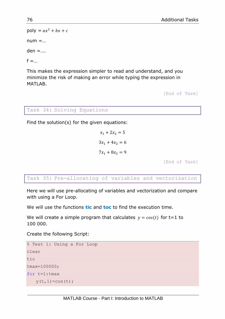
Task 35: Pre-allocating of variables and vectorization
Here we will use pre-allocating of variables and vectorization and compare
with using a For Loop.
We will use the functions tic and toc to find the execution time.
We will create a simple program that calculates 𝑦 = 𝑐𝑜𝑠(𝑡) for t=1 to
100 000.
Create the following Script:
% Test 1: Using a For Loop
clear
tic
tmax=100000;
for t=1:tmax
y(t,1)=cos(t);
77 Additional Tasks
MATLAB Course - Part I: Introduction to MATLAB
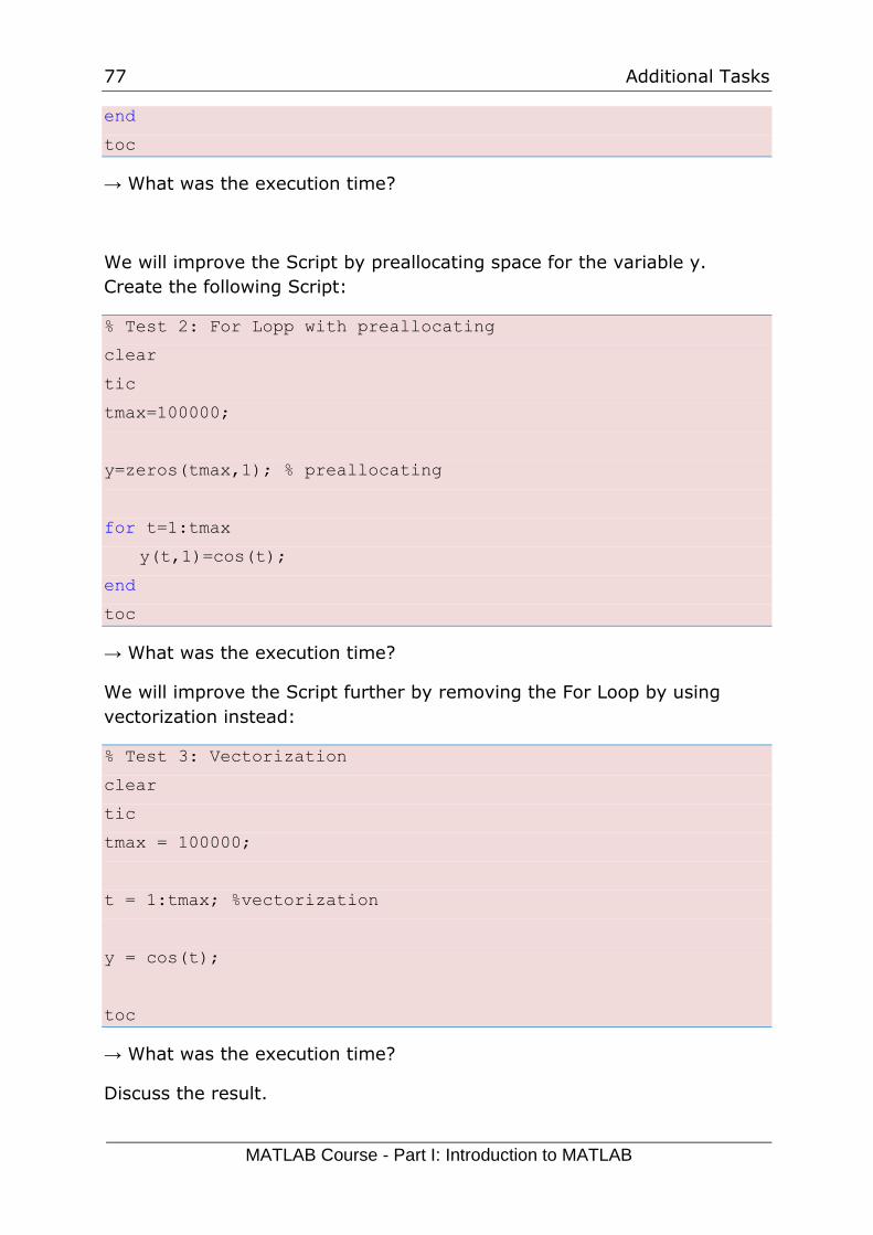
end
toc
→ What was the execution time?
We will improve the Script by preallocating space for the variable y.
Create the following Script:
% Test 2: For Lopp with preallocating
clear
tic
tmax=100000;
y=zeros(tmax,1); % preallocating
for t=1:tmax
y(t,1)=cos(t);
end
toc
→ What was the execution time?
We will improve the Script further by removing the For Loop by using
vectorization instead:
% Test 3: Vectorization
clear
tic
tmax = 100000;
t = 1:tmax; %vectorization
y = cos(t);
toc
→ What was the execution time?
Discuss the result.
78 Additional Tasks
MATLAB Course - Part I: Introduction to MATLAB
[End of Task]
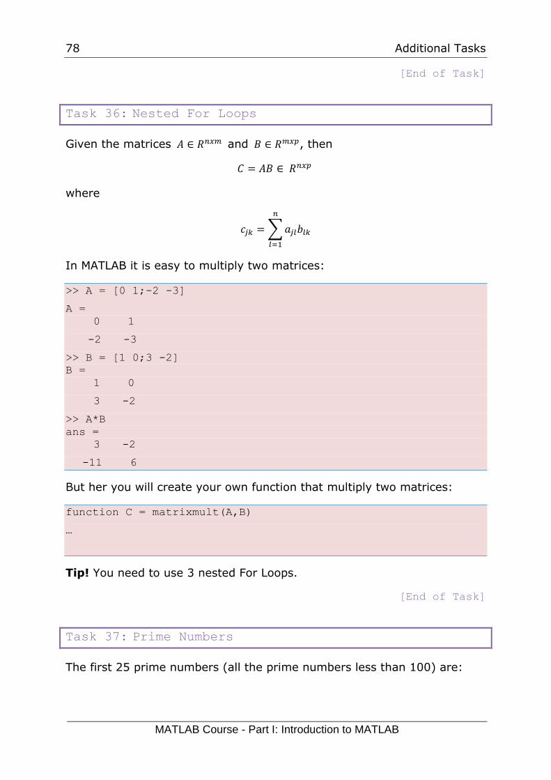
Task 36: Nested For Loops
Given the matrices 𝐴 ∈ 𝑅𝑛𝑥𝑚 and 𝐵 ∈ 𝑅𝑚𝑥𝑝, then
𝐶 = 𝐴𝐵 ∈ 𝑅𝑛𝑥𝑝
where
𝑐𝑗𝑘 =∑𝑎𝑗𝑙𝑏𝑙𝑘
𝑛
𝑙=1
In MATLAB it is easy to multiply two matrices:
>> A = [0 1;-2 -3]
A =
0 1
-2 -3
>> B = [1 0;3 -2]
B =
1 0
3 -2
>> A*B
ans =
3 -2
-11 6
But her you will create your own function that multiply two matrices:
function C = matrixmult(A,B)
…
Tip! You need to use 3 nested For Loops.
[End of Task]
Task 37: Prime Numbers
The first 25 prime numbers (all the prime numbers less than 100) are:
79 Additional Tasks
MATLAB Course - Part I: Introduction to MATLAB
2, 3, 5, 7, 11, 13, 17, 19, 23, 29, 31, 37, 41, 43, 47, 53, 59, 61, 67, 71,
73, 79, 83, 89, 97
By definition a prime number has both 1 and itself as a divisor. If it has
any other divisor, it cannot be prime.
A natural number (1, 2, 3, 4, 5, 6, etc.) is called a prime number (or a
prime) if it is greater than 1 and cannot be written as a product of two
natural numbers that are both smaller than it.
Create a MATLAB Script where you find all prime numbers between 1 and
200.
Tip! I guess this can be done in many different ways, but one way is to
use 2 nested For Loops.
[End of Task]
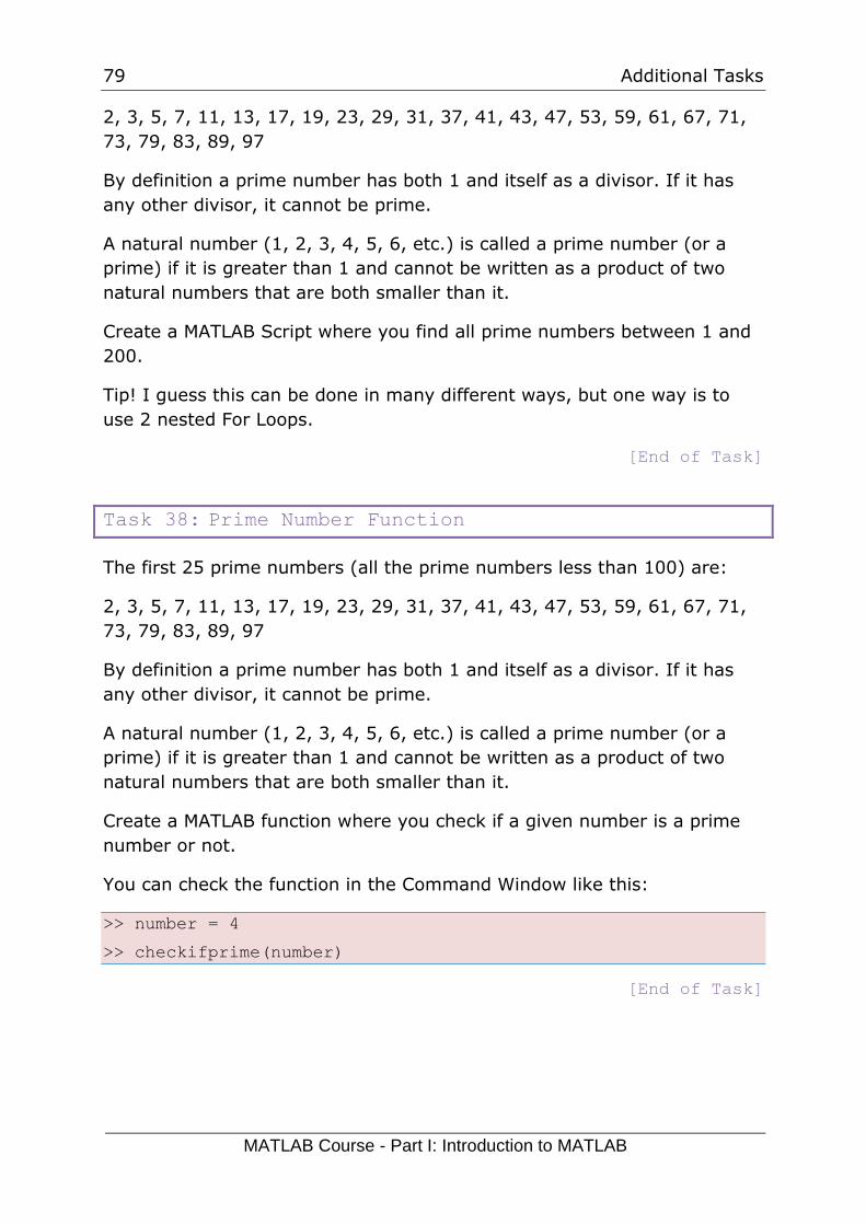
Task 38: Prime Number Function
The first 25 prime numbers (all the prime numbers less than 100) are:
2, 3, 5, 7, 11, 13, 17, 19, 23, 29, 31, 37, 41, 43, 47, 53, 59, 61, 67, 71,
73, 79, 83, 89, 97
By definition a prime number has both 1 and itself as a divisor. If it has
any other divisor, it cannot be prime.
A natural number (1, 2, 3, 4, 5, 6, etc.) is called a prime number (or a
prime) if it is greater than 1 and cannot be written as a product of two
natural numbers that are both smaller than it.
Create a MATLAB function where you check if a given number is a prime
number or not.
You can check the function in the Command Window like this:
>> number = 4
>> checkifprime(number)
[End of Task]

80 Additional Tasks
MATLAB Course - Part I: Introduction to MATLAB
81
Appendix A: MATLAB
Functions
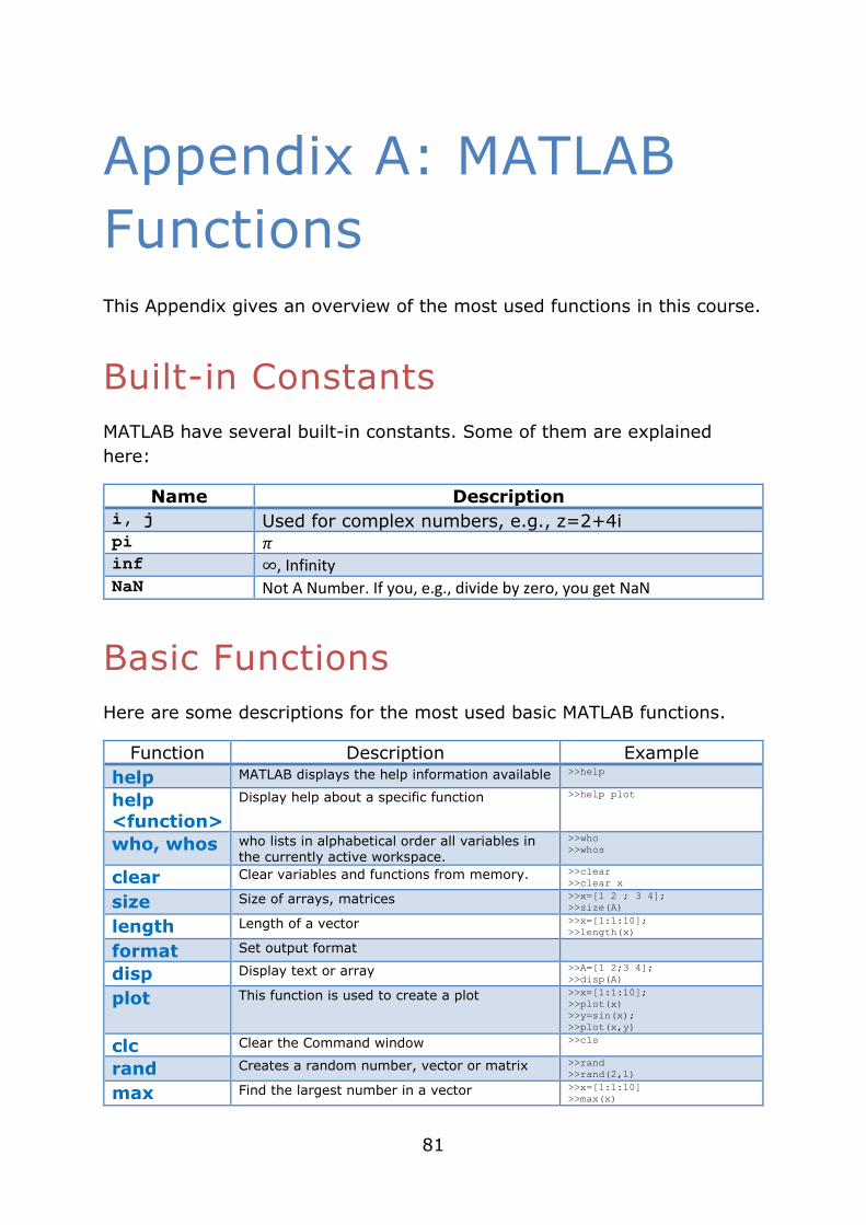
This Appendix gives an overview of the most used functions in this course.
Built-in Constants
MATLAB have several built-in constants. Some of them are explained
here:
Name Description
i, j Used for complex numbers, e.g., z=2+4i pi 𝜋 inf ∞, Infinity NaN Not A Number. If you, e.g., divide by zero, you get NaN
Basic Functions
Here are some descriptions for the most used basic MATLAB functions.
Function Description Example
help MATLAB displays the help information available >>help
help
<function>
Display help about a specific function >>help plot
who, whos who lists in alphabetical order all variables in the currently active workspace.
>>who
>>whos
clear Clear variables and functions from memory. >>clear
>>clear x
size Size of arrays, matrices >>x=[1 2 ; 3 4];
>>size(A)
length Length of a vector >>x=[1:1:10];
>>length(x)
format Set output format
disp Display text or array >>A=[1 2;3 4];
>>disp(A)
plot This function is used to create a plot >>x=[1:1:10];
>>plot(x)
>>y=sin(x);
>>plot(x,y)
clc Clear the Command window >>cls
rand Creates a random number, vector or matrix >>rand
>>rand(2,1)
max Find the largest number in a vector >>x=[1:1:10]
>>max(x)
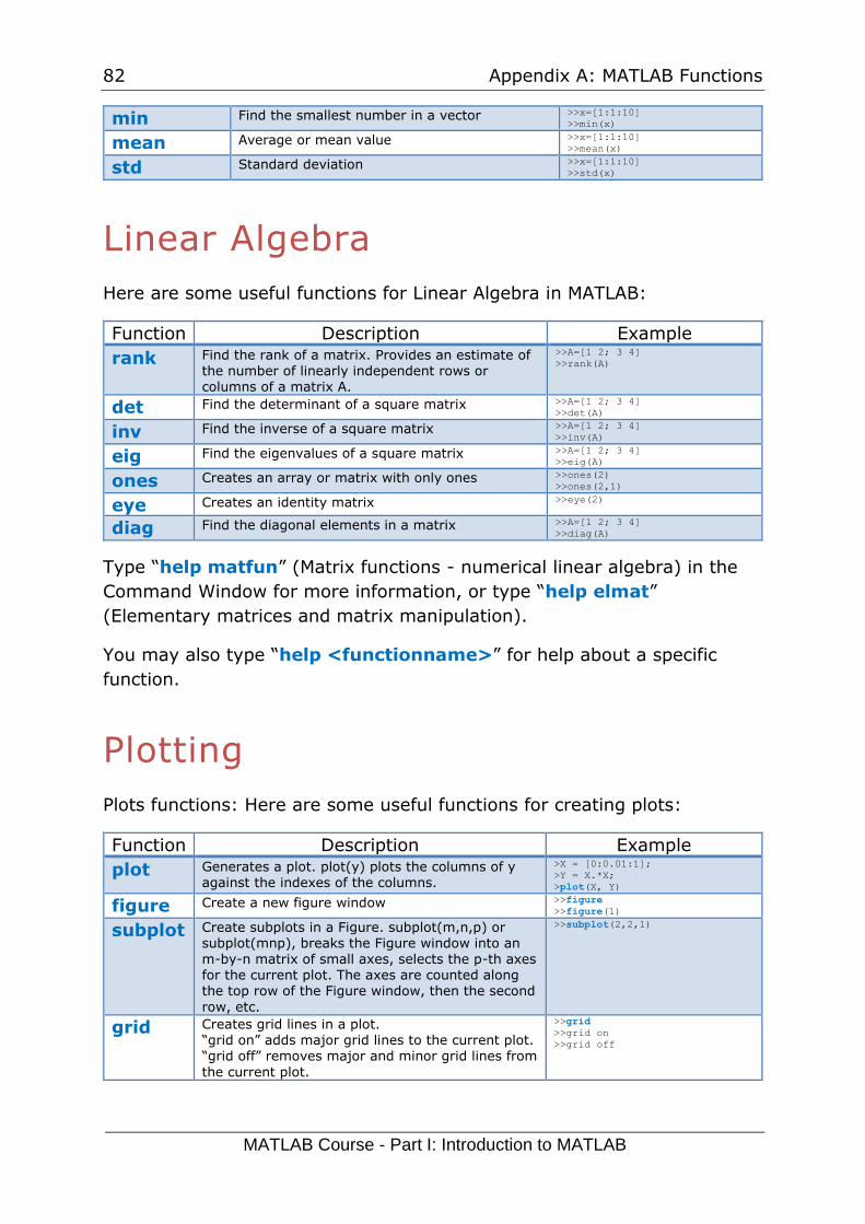
82 Appendix A: MATLAB Functions
MATLAB Course - Part I: Introduction to MATLAB
min Find the smallest number in a vector >>x=[1:1:10]
>>min(x)
mean Average or mean value >>x=[1:1:10]
>>mean(x)
std Standard deviation >>x=[1:1:10]
>>std(x)
Linear Algebra
Here are some useful functions for Linear Algebra in MATLAB:
Function Description Example
rank Find the rank of a matrix. Provides an estimate of the number of linearly independent rows or columns of a matrix A.
>>A=[1 2; 3 4]
>>rank(A)
det Find the determinant of a square matrix >>A=[1 2; 3 4]
>>det(A)
inv Find the inverse of a square matrix >>A=[1 2; 3 4]
>>inv(A)
eig Find the eigenvalues of a square matrix >>A=[1 2; 3 4]
>>eig(A)
ones Creates an array or matrix with only ones >>ones(2)
>>ones(2,1)
eye Creates an identity matrix >>eye(2)
diag Find the diagonal elements in a matrix >>A=[1 2; 3 4]
>>diag(A)
Type “help matfun” (Matrix functions - numerical linear algebra) in the
Command Window for more information, or type “help elmat”
(Elementary matrices and matrix manipulation).
You may also type “help <functionname>” for help about a specific
function.
Plotting
Plots functions: Here are some useful functions for creating plots:
Function Description Example
plot Generates a plot. plot(y) plots the columns of y against the indexes of the columns.
>X = [0:0.01:1];
>Y = X.*X;
>plot(X, Y)
figure Create a new figure window >>figure
>>figure(1)
subplot Create subplots in a Figure. subplot(m,n,p) or subplot(mnp), breaks the Figure window into an
m-by-n matrix of small axes, selects the p-th axes for the current plot. The axes are counted along the top row of the Figure window, then the second
row, etc.
>>subplot(2,2,1)
grid Creates grid lines in a plot. “grid on” adds major grid lines to the current plot. “grid off” removes major and minor grid lines from
the current plot.
>>grid
>>grid on
>>grid off
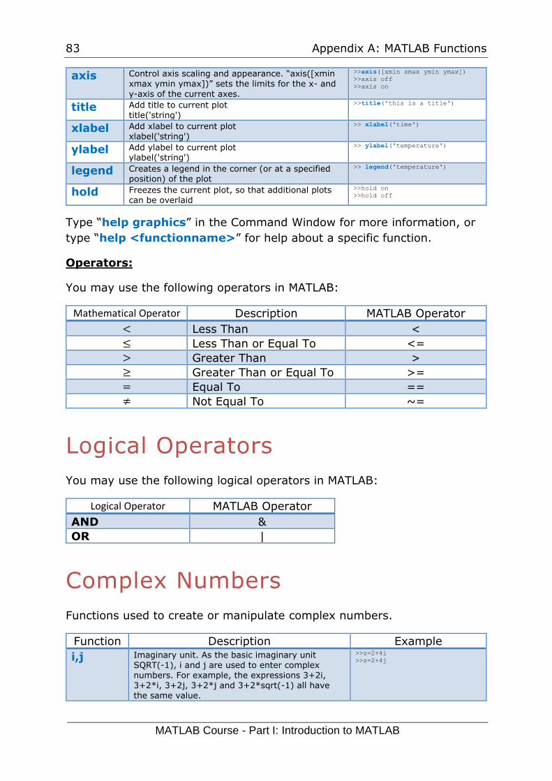
83 Appendix A: MATLAB Functions
MATLAB Course - Part I: Introduction to MATLAB
axis Control axis scaling and appearance. “axis([xmin
xmax ymin ymax])” sets the limits for the x- and
y-axis of the current axes.
>>axis([xmin xmax ymin ymax])
>>axis off
>>axis on
title Add title to current plot title('string')
>>title('this is a title')
xlabel Add xlabel to current plot xlabel('string')
>> xlabel('time')
ylabel Add ylabel to current plot ylabel('string')
>> ylabel('temperature')
legend Creates a legend in the corner (or at a specified position) of the plot
>> legend('temperature')
hold Freezes the current plot, so that additional plots can be overlaid
>>hold on
>>hold off
Type “help graphics” in the Command Window for more information, or
type “help <functionname>” for help about a specific function.
Operators:
You may use the following operators in MATLAB:
Mathematical Operator Description MATLAB Operator
< Less Than <
≤ Less Than or Equal To <=
> Greater Than >
≥ Greater Than or Equal To >=
= Equal To ==
≠ Not Equal To ~=
Logical Operators
You may use the following logical operators in MATLAB:
Logical Operator MATLAB Operator
AND &
OR |
Complex Numbers
Functions used to create or manipulate complex numbers.
Function Description Example
i,j Imaginary unit. As the basic imaginary unit SQRT(-1), i and j are used to enter complex numbers. For example, the expressions 3+2i, 3+2*i, 3+2j, 3+2*j and 3+2*sqrt(-1) all have the same value.
>>z=2+4i
>>z=2+4j
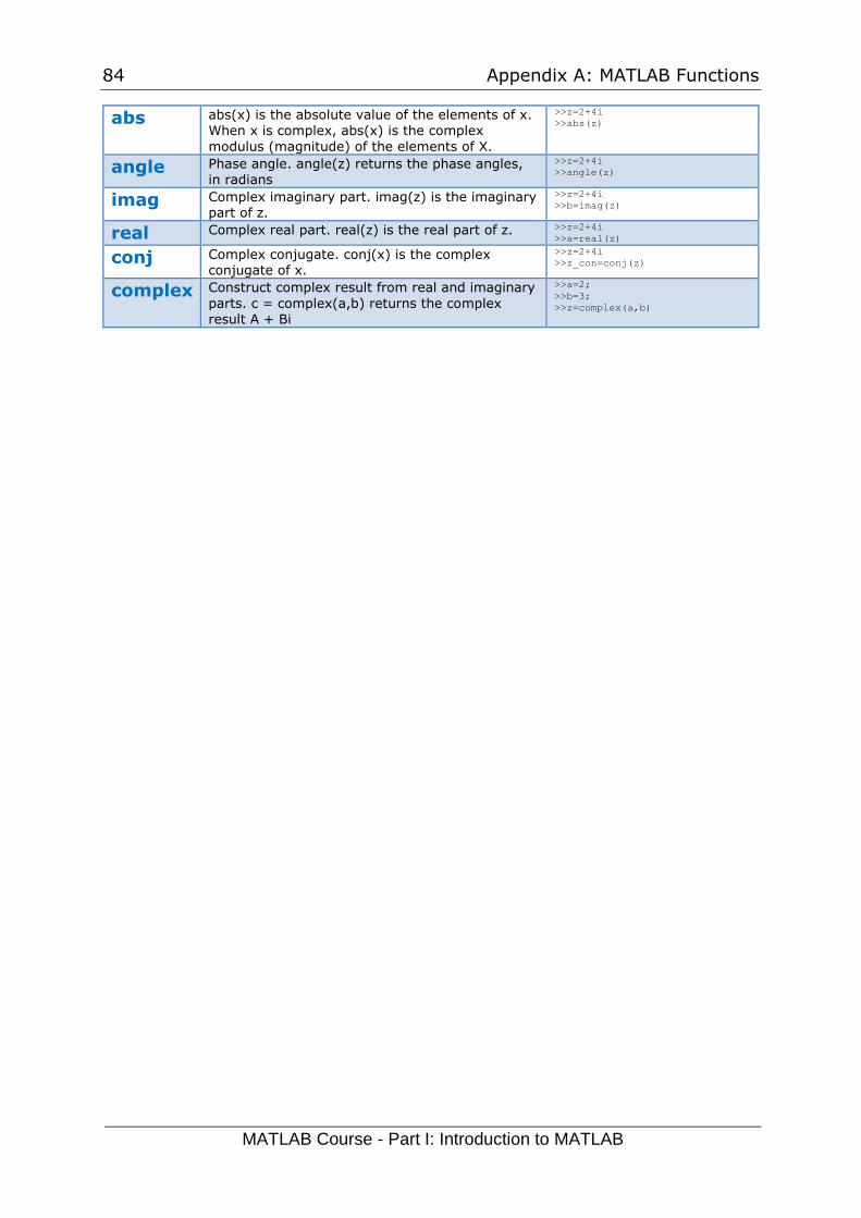
84 Appendix A: MATLAB Functions
MATLAB Course - Part I: Introduction to MATLAB
abs abs(x) is the absolute value of the elements of x.
When x is complex, abs(x) is the complex
modulus (magnitude) of the elements of X.
>>z=2+4i
>>abs(z)
angle Phase angle. angle(z) returns the phase angles, in radians
>>z=2+4i
>>angle(z)
imag Complex imaginary part. imag(z) is the imaginary part of z.
>>z=2+4i
>>b=imag(z)
real Complex real part. real(z) is the real part of z. >>z=2+4i
>>a=real(z)
conj Complex conjugate. conj(x) is the complex conjugate of x.
>>z=2+4i
>>z_con=conj(z)
complex Construct complex result from real and imaginary
parts. c = complex(a,b) returns the complex result A + Bi
>>a=2;
>>b=3;
>>z=complex(a,b)

Hans-Petter Halvorsen
E-mail: [email protected]
Blog: http://www.halvorsen.blog
University of South-Eastern Norway
www.usn.no

Introduction to MATLAB