Introduction to MATLAB

Simon O’Keefe

Non-Standard Computation Group

sok@cs.york.ac.uk

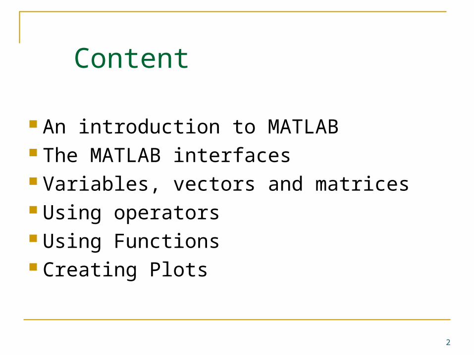
Content

An introduction to MATLAB The MATLAB interfaces Variables, vectors and matrices Using operators Using Functions Creating Plots

2

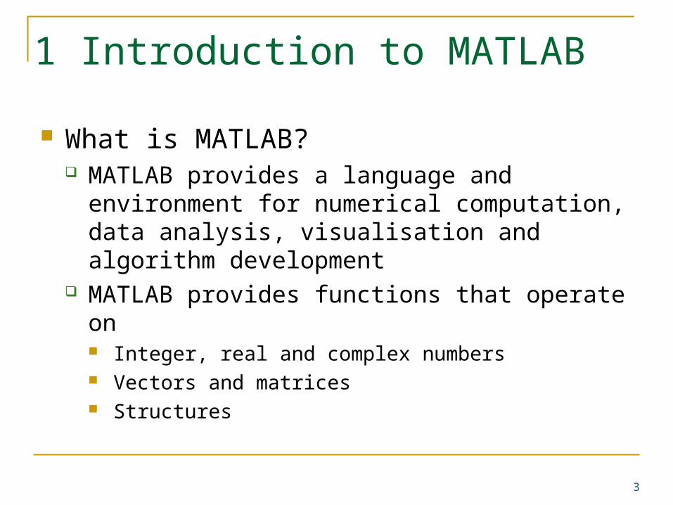
1 Introduction to MATLAB

What is MATLAB? MATLAB provides a language and environment

for numerical computation, data analysis, visualisation and algorithm development

MATLAB provides functions that operate on Integer, real and complex numbers Vectors and matrices Structures

3

1 MATLAB Functionality

Built-in Functionality includes Matrix manipulation and linear algebra Data analysis Graphics and visualisation …and hundreds of other functions

Add-on toolboxes provide* Image processing Signal Processing Optimization Genetic Algorithms…* but we have to pay for these extras

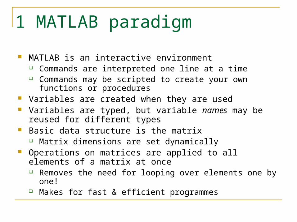
1 MATLAB paradigm

MATLAB is an interactive environment Commands are interpreted one line at a time Commands may be scripted to create your own functions or

procedures Variables are created when they are used Variables are typed, but variable names may be reused for

different types Basic data structure is the matrix

Matrix dimensions are set dynamically Operations on matrices are applied to all elements of a matrix at

once Removes the need for looping over elements one by one! Makes for fast & efficient programmes

1 Starting and stopping

To Start On Windows XP platform select Start->Programs->Maths and Stats->

MATLAB->MATLAB_local->R2007a->MATLAB R2007a For access to the Genetic Algorithms and Stats

toolboxes, you must use R2007b on Windows MATLAB runs on Linux quite happily but we do not have

toolbox licences

To stop (nicely) Select File -> Exit MATLAB Or type quit in the MATLAB command window

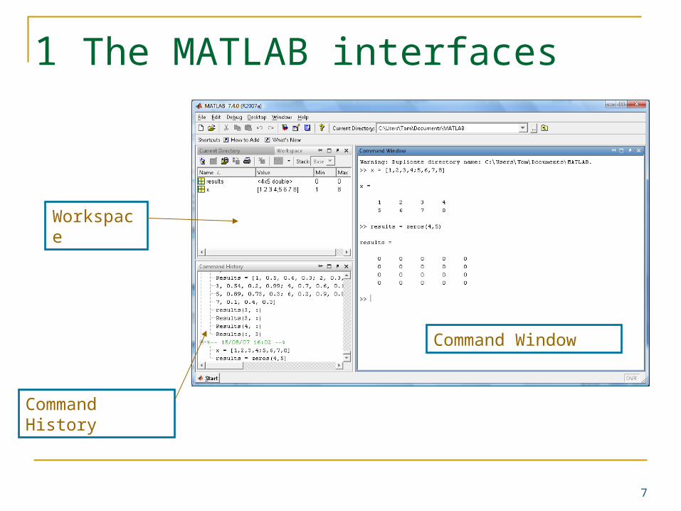
1 The MATLAB interfaces

7

Command Window

Workspace

Command History

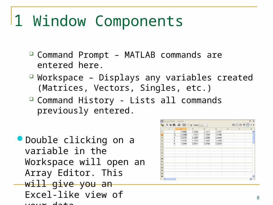
1 Window Components

Command Prompt – MATLAB commands are entered here.

Workspace – Displays any variables created (Matrices, Vectors, Singles, etc.)

Command History - Lists all commands previously entered.

Double clicking on a variable in the Workspace will open an Array Editor. This will give you an Excel-like view of your data.

8

1 The MATLAB Interface

Pressing the up arrow in the command window will bring up the last command entered This saves you time when things go wrong

If you want to bring up a command from some time in the past type the first letter and press the up arrow.

The current working directory should be set to a directory of your own

9

2 Variables, vectors and matrices

10

2.1 Creating Variables Variables

Names Can be any string of upper and lower case letters along with

numbers and underscores but it must begin with a letter Reserved names are IF, WHILE, ELSE, END, SUM, etc. Names are case sensitive

Value This is the data the is associated to the variable; the data is

accessed by using the name. Variables have the type of the last thing assigned to

them Re-assignment is done silently – there are no warnings if you

overwrite a variable with something of a different type.

11

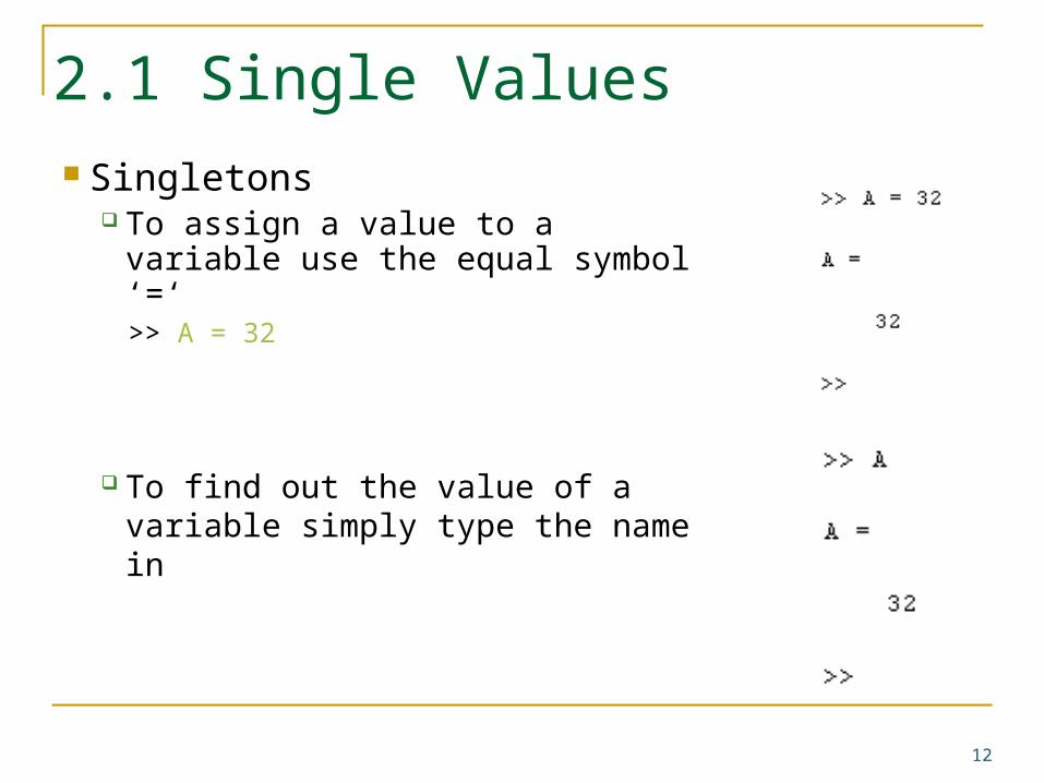
2.1 Single Values Singletons

To assign a value to a variable use the equal symbol ‘=‘>> A = 32

To find out the value of a variable simply type the name in

12

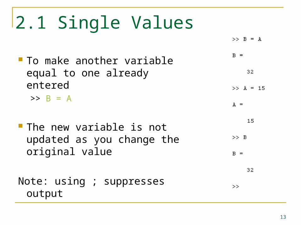
2.1 Single Values

To make another variable equal to one already entered>> B = A

The new variable is not updated as you change the original value

Note: using ; suppresses output

13

2.1 Single Values

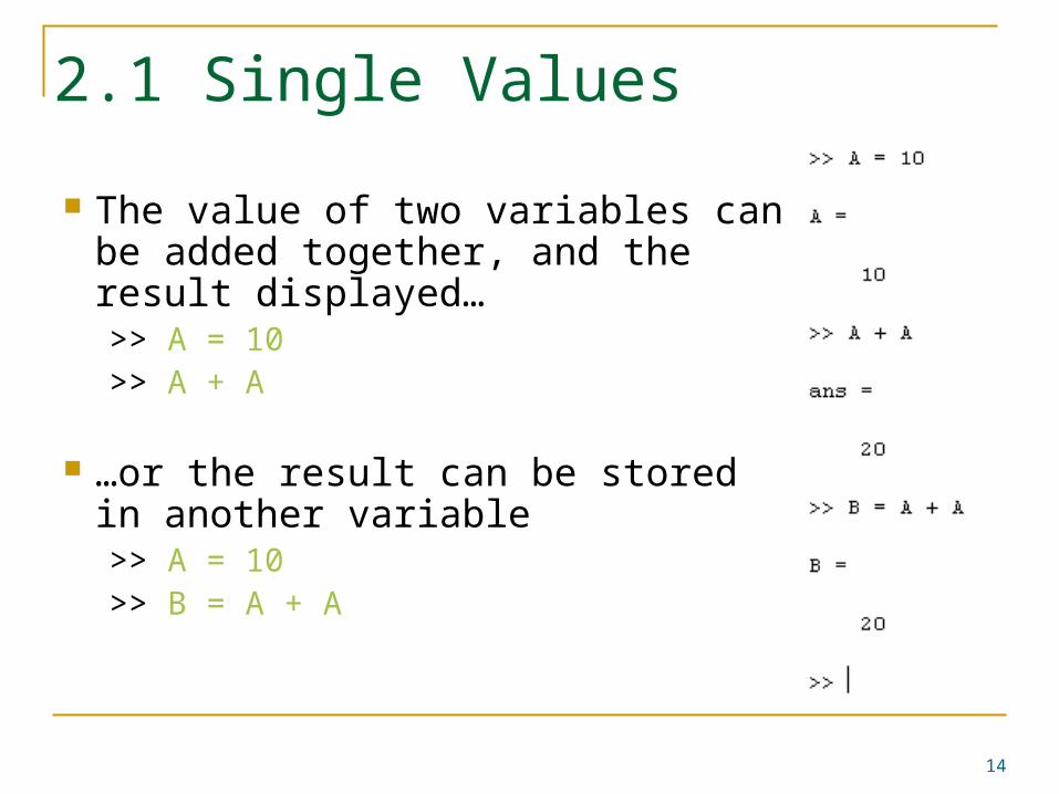
The value of two variables can be added together, and the result displayed…>> A = 10>> A + A

…or the result can be stored in another variable>> A = 10>> B = A + A

14

2.1 Vectors

A vector is a list of numbers Use square brackets [] to contain the numbers

To create a row vector use ‘,’ to separate the content

15

2.1 Vectors

To create a column vector use ‘;’ to separate the content

16

2.1 Vectors A row vector can be converted into a column vector

by using the transpose operator ‘

17

2.1 Matrices

A MATLAB matrix is a rectangular array of numbers Scalars and vectors are regarded as special cases of

matrices MATLAB allows you to work with a whole array at a time

2.1 Matrices

You can create matrices (arrays) of any size using a combination of the methods for creating vectors

List the numbers using ‘,’ to separate each column and then ‘;’ to define a new row

19

2.1 Matrices

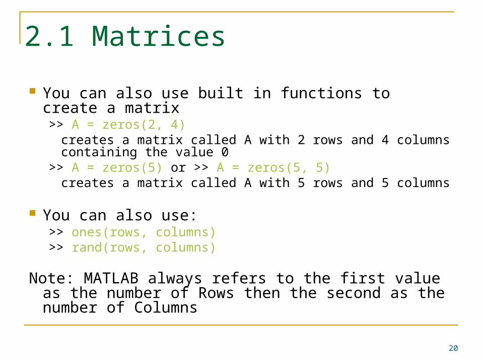
You can also use built in functions to create a matrix>> A = zeros(2, 4)

creates a matrix called A with 2 rows and 4 columns containing the value 0

>> A = zeros(5) or >> A = zeros(5, 5) creates a matrix called A with 5 rows and 5 columns

You can also use:>> ones(rows, columns)>> rand(rows, columns)

Note: MATLAB always refers to the first value as the number of Rows then the second as the number of Columns

20

2.1 Clearing Variables

You can use the command “clear all” to delete all the variables present in the workspace

You can also clear specific variables using:>> clear Variable_Name

21

2.2 Accessing Matrix Elements

An Element is a single number within a matrix or vector

To access elements of a matrix type the matrices’ name followed by round brackets containing a reference to the row and column number:

>> Variable_Name(Row_Number, Column_Number)

NOTE: In Excel you reference a value by Column, Row. In MATLAB you reference a value by Row, Column

22

2.2 Accessing Matrix Elements

To access Subject 3’s result for Test 3 In Excel (Column, Row):

D3 In MATLAB (Row, Column):

>> results(3, 4)

Excel MATLAB

2nd 1st

1st 2nd

23

2.2 Changing Matrix Elements

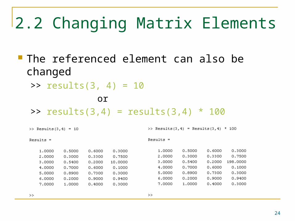
The referenced element can also be changed>> results(3, 4) = 10

or

>> results(3,4) = results(3,4) * 100

24

2.2 Accessing Matrix Rows

You can also access multiple values from a Matrix using the : symbol To access all columns of a row enter:

>> Variable_Name(RowNumber, :)

25

2.2 Accessing Matrix Columns

To access all rows of a column >> Variable_Name(:, ColumnNumber)

26

2.2 Changing Matrix Rows or Columns

These reference methods can be used to change the values of multiple matrix elements

To change all of the values in a row or column to zero use

>> results(:, 3) = 0 >> results(:, 5) = results(:, 3) + results(:, 4)

27

2.2 Changing Matrix Rows or Columns

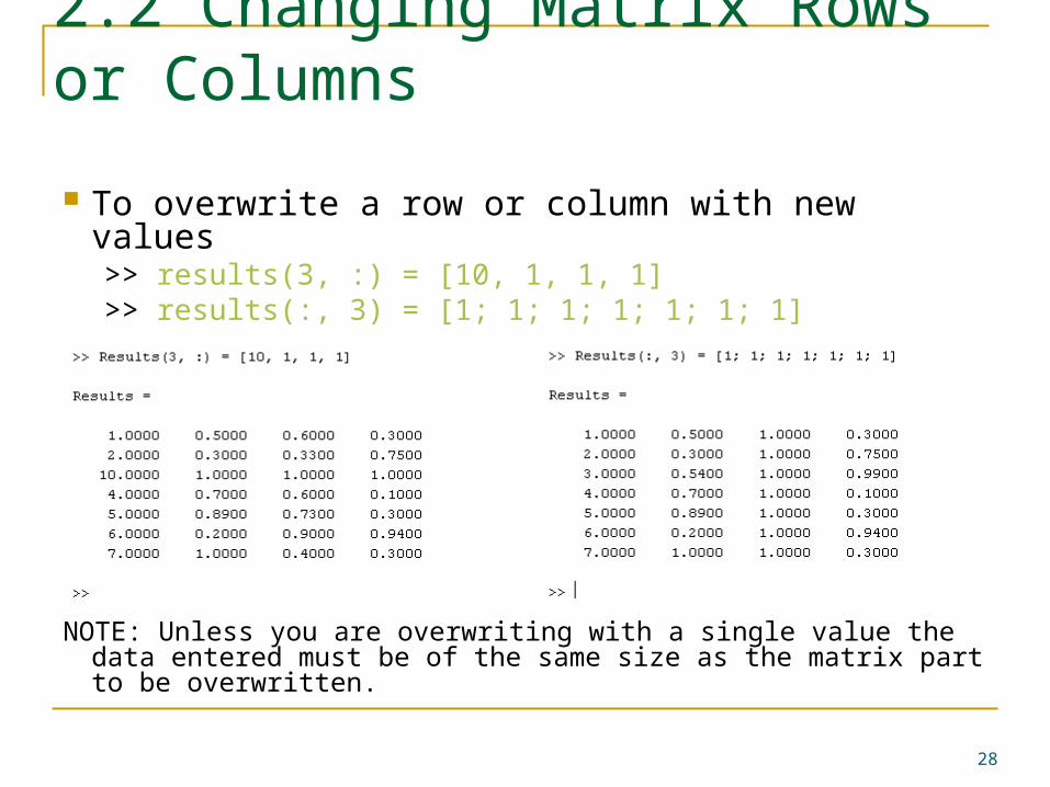
To overwrite a row or column with new values>> results(3, :) = [10, 1, 1, 1]>> results(:, 3) = [1; 1; 1; 1; 1; 1; 1]

NOTE: Unless you are overwriting with a single value the data entered must be of the same size as the matrix part to be overwritten.

28

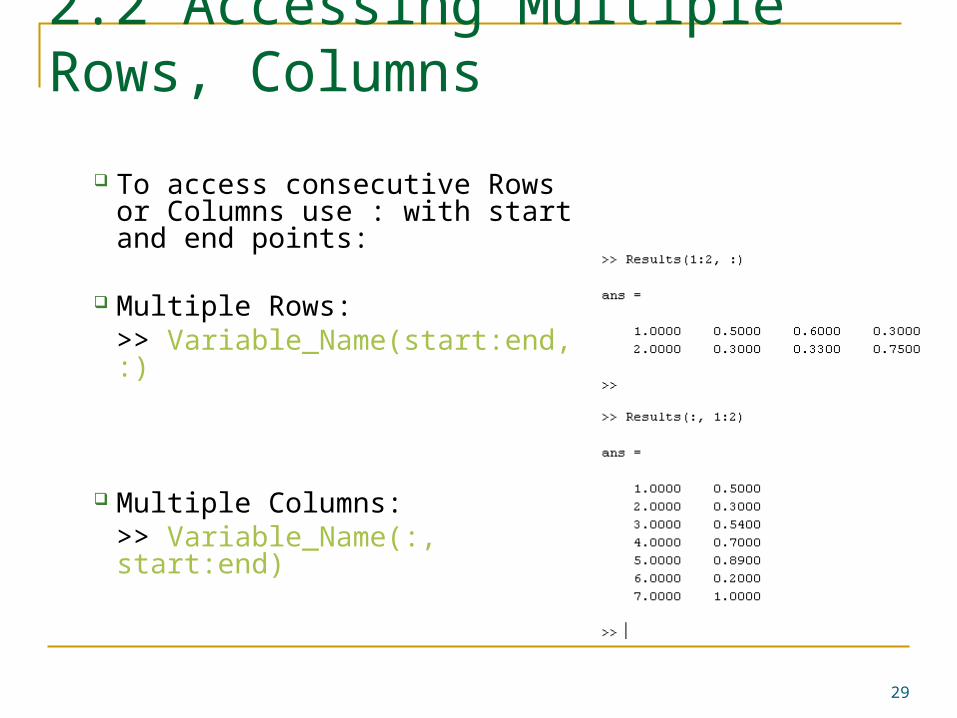
2.2 Accessing Multiple Rows, Columns

To access consecutive Rows or Columns use : with start and end points:

Multiple Rows: >> Variable_Name(start:end, :)

Multiple Columns: >> Variable_Name(:, start:end)

29

2.2 Accessing Multiple Rows, Columns

To access multiple non consecutive Rows or Columns use a vector of indexes (using square brackets [])

Multiple Rows: >>Variable_Name([index1, index2, etc.], :)

Multiple Columns: >>Variable_Name(:, [index1, index2, etc.])

30

2.2 Changing Multiple Rows, Columns

The same referencing can be used to change multiple Rows or Columns

>> results(3:6, :) = 0>> results([3,6], :) = 0

31

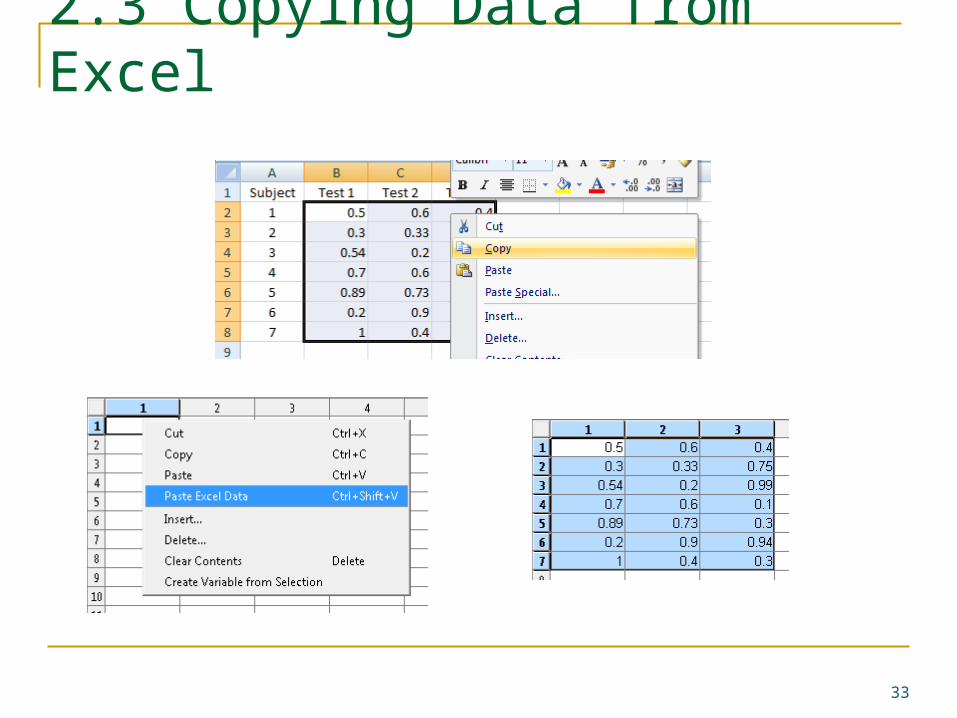
2.3 Copying Data from Excel

MATLAB’s Array Editor allows you to copy data from an Excel spreadsheet in a very simple way

In Excel select the data and click on copy

Double click on the variable you would like to store the data in This will open the array editor

In the Array Editor right click in the first element and select “Paste Excel Data”

32

2.3 Copying Data from Excel

33

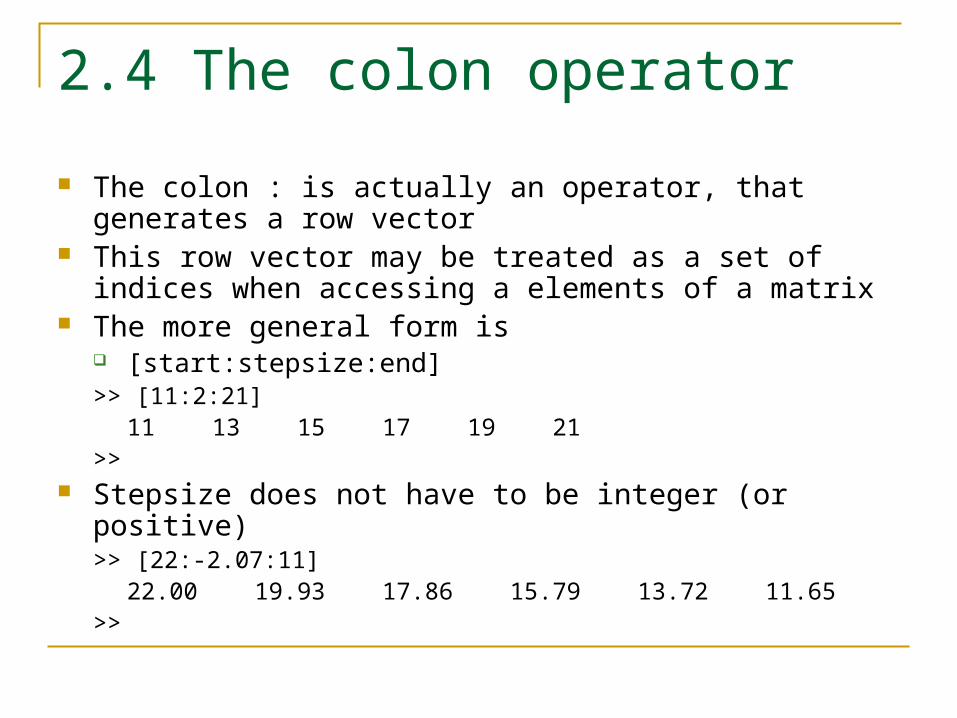
2.4 The colon operator

The colon : is actually an operator, that generates a row vector

This row vector may be treated as a set of indices when accessing a elements of a matrix

The more general form is [start:stepsize:end]>> [11:2:21]

11 13 15 17 19 21>>

Stepsize does not have to be integer (or positive)>> [22:-2.07:11]

22.00 19.93 17.86 15.79 13.72 11.65>>

2.4 Concatenation

The square brackets [] are the concatenation operator.

So far, we have concatenated single elements to form a vector or matrix.

The operator is more general than that – for example we can concatenate matrices (with the same dimension) to form a larger matrix

2.4 Saving and Loading Data

Variables that are currently in the workspace can be saved and loaded using the save and load commands

MATLAB will save the file in the Current Directory

To save the variables use>> save File_Name [variable variable …]

To load the variables use>> load File_Name [variable variable …]

36

3 More Operators

37

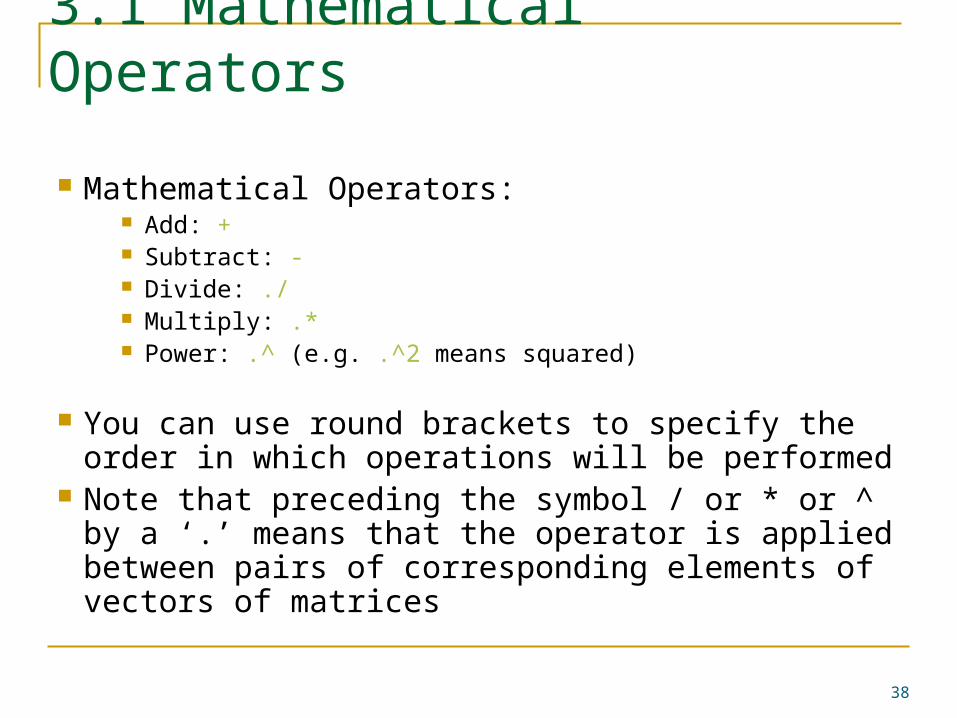
3.1 Mathematical Operators

Mathematical Operators: Add: + Subtract: - Divide: ./ Multiply: .* Power: .^ (e.g. .^2 means squared)

You can use round brackets to specify the order in which operations will be performed

Note that preceding the symbol / or * or ^ by a ‘.’ means that the operator is applied between pairs of corresponding elements of vectors of matrices

38

3.1 Mathematical Operators

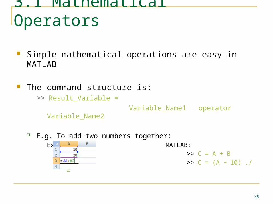
Simple mathematical operations are easy in MATLAB

The command structure is:>> Result_Variable =

Variable_Name1 operator Variable_Name2

E.g. To add two numbers together:Excel: MATLAB:

>> C = A + B

>> C = (A + 10) ./ 2

39

3.1 Mathematical Operators

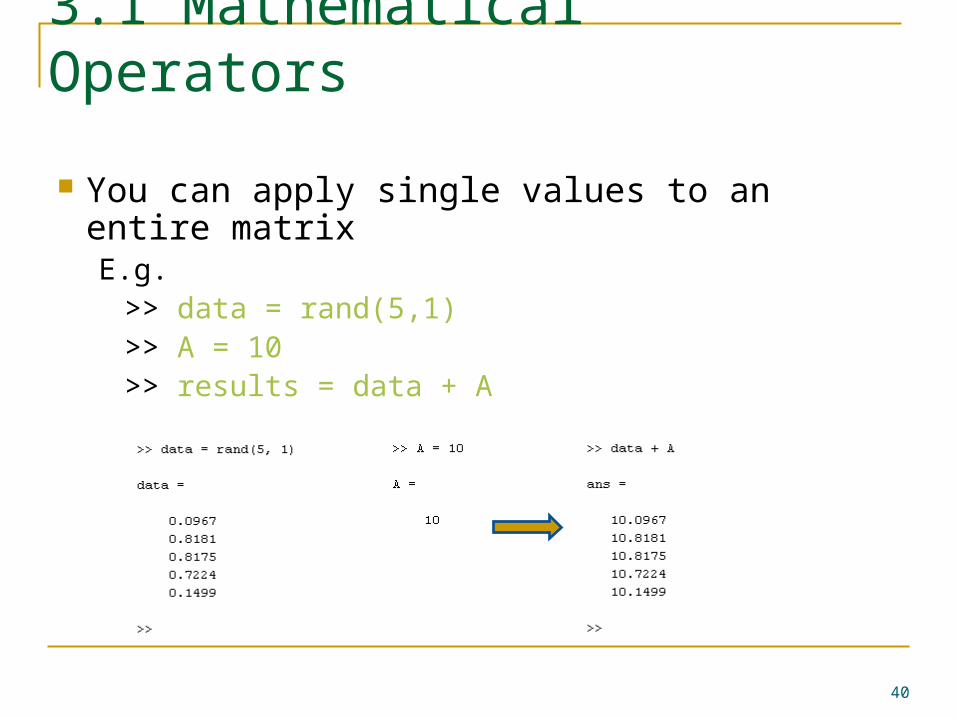
You can apply single values to an entire matrixE.g.

>> data = rand(5,1)>> A = 10>> results = data + A

40

3.1 Mathematical Operators

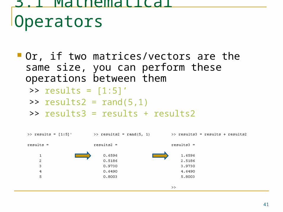
Or, if two matrices/vectors are the same size, you can perform these operations between them>> results = [1:5]’>> results2 = rand(5,1)>> results3 = results + results2

41

3.1 Mathematical Operators Combining this with methods from Accessing Matrix Elements

gives way to more useful operations>> results = zeros(3, 5)

>> results(:, 1:4) = rand(3, 4)

>> results(:, 5) = results(:, 1) + results(:, 2) + results(:, 3) + results(:, 4)

or

>> results(:, 5) = results(:, 1) .* results(:, 2) .* results(:, 3) .* results(:, 4)

NOTE: There is a simpler way to do this using the Sum and Prod functions, this will be shown later.

42

3.1 Mathematical Operators

43

>> results(:, 1:4) = rand(3, 4)>> results(:, 5) = results(:, 1) + results(:, 2) + results(:, 3) + results(:, 4)

>> results = zeros(3, 5)

3.1 Mathematical Operators

You can perform operations on a matrix - you are very likely to use these Matrix Operators:

Matrix Multiply: * Matrix Right Division: /

Example:

44

3.1 Operation on matrices

Multiplication of matrices with * calculates inner products between rows and columns

To transpose a matrix, use ‘ det(A) calculates the determinant of a matrix A inv(A) calculates the inverse of a matrix A pinv(A) calculates the pseudo-inverse of A …and so on

3.2 Logical Operators

You can use Logical Indexing to find data that conforms to some limitations

Logical Operators: Greater Than: > Less Than: < Greater Than or Equal To: >= Less Than or Equal To: <= Is Equal: == Not Equal To: ~=

46

3.2 Logical Indexing

For example, you can find data that is above a certain limit:>> r = results(:,1)

>> ind = r > 0.2

>> r(ind)

ind is the same size as r and contains zeros (false) where the data does not fit the criteria and ones (true) where it does, this is called a Logical Vector.

r(ind) then extracts the data where ones exist in ind

47

3.2 Logical Indexing

48

>> r = results(:,1)>> ind = r > 0.2

>> r(ind)

3.3 Boolean Operators

Boolean Operators: AND: & OR: | NOT: ~

Connects two logical expressions together

49

3.3 Boolean Operators

Using a combination of Logical and Boolean operators we can select values that fall within a lower and upper limit>> r = results(:,1)

>> ind = r > 0.2 & r <= 0.9

>> r(ind)

More later...

50

4 Functions

51

4 Functions

A function performs an operation on the input variable you pass to it

Passing variables is easy, you just list them within round brackets when you call the function

function_Name(input)

You can also pass the function parts of a matrix>> function_Name(matrix(:, 1))

or>> function_Name(matrix(:, 2:4))

52

4 Functions

The result of the function can be stored in a variable>> output_Variable = function_Name(input)

e.g.

>> mresult = mean(results)

You can also tell the function to store the result in parts of a matrix>> matrix(:, 5) = function_Name(matrix(:, 1:4))

53

4 Functions

To get help with using a function enter>> help function_Name

This will display information on how to use the function and what it does

54

4 Functions

MATLAB has many built in functions which make it easy to perform a variety of statistical operations

sum – Sums the content of the variable passed prod – Multiplies the content of the variable passed mean – Calculates the mean of the variable passed median – Calculates the median of the variable passed mode – Calculates the Mode of the variable passed std – Calculates the standard deviation of the variable passed sqrt – Calculates the square root of the variable passed max – Finds the maximum of the data min – Finds the minimum of the data size – Gives the size of the variable passed

55

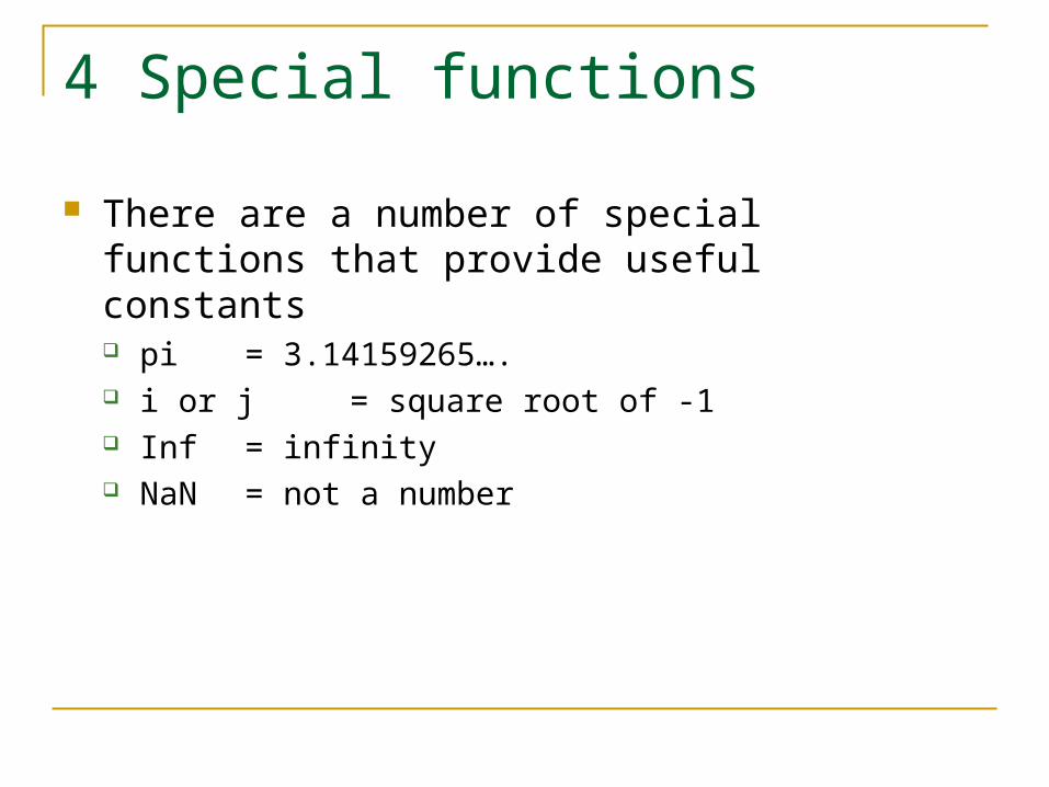
4 Special functions

There are a number of special functions that provide useful constants pi = 3.14159265…. i or j = square root of -1 Inf = infinity NaN = not a number

4 Functions

Passing a vector to a function like sum, mean, std will calculate the property within the vector

>> sum([1,2,3,4,5])

= 15

>> mean([1,2,3,4,5])

= 3

57

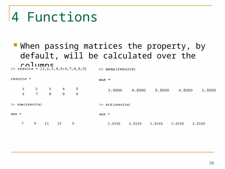
4 Functions

When passing matrices the property, by default, will be calculated over the columns

58

4 Functions

To change the direction of the calculation to the other dimension (columns) use:>> function_Name(input, 2)

When using std, max and min you need to write:>> function_Name(input, [], 2)

59

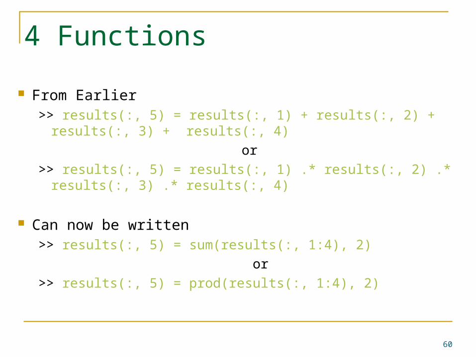
4 Functions

From Earlier>> results(:, 5) = results(:, 1) + results(:, 2) + results(:, 3) + results(:, 4)

or

>> results(:, 5) = results(:, 1) .* results(:, 2) .* results(:, 3) .* results(:, 4)

Can now be written>> results(:, 5) = sum(results(:, 1:4), 2)

or

>> results(:, 5) = prod(results(:, 1:4), 2)

60

4 Functions More usefully you

can now take the mean and standard deviation of the data, and add them to the array

61

4 Functions

You can find the maximum and minimum of some data using the max and min functions>> max(results)

>> min(results)

62

4 Functions

We can use functions and logical indexing to extract all the results for a subject that fall between 2 standard deviations of the mean>> r = results(:,1)

>> ind = (r > mean(r) – 2*std(r)) & (r < mean(r) + 2*std(r))

>> r(ind)

63

5 Plotting

64

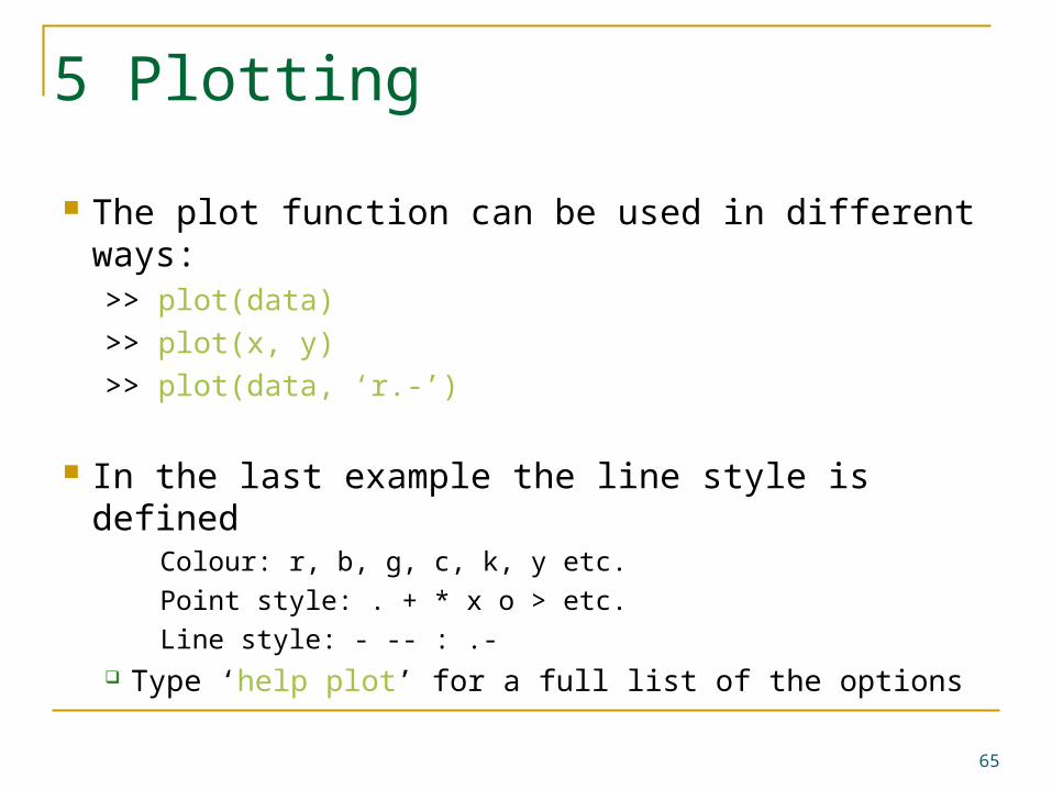
5 Plotting

The plot function can be used in different ways:>> plot(data)

>> plot(x, y)

>> plot(data, ‘r.-’)

In the last example the line style is definedColour: r, b, g, c, k, y etc.

Point style: . + * x o > etc.

Line style: - -- : .- Type ‘help plot’ for a full list of the options

65

5 Plotting

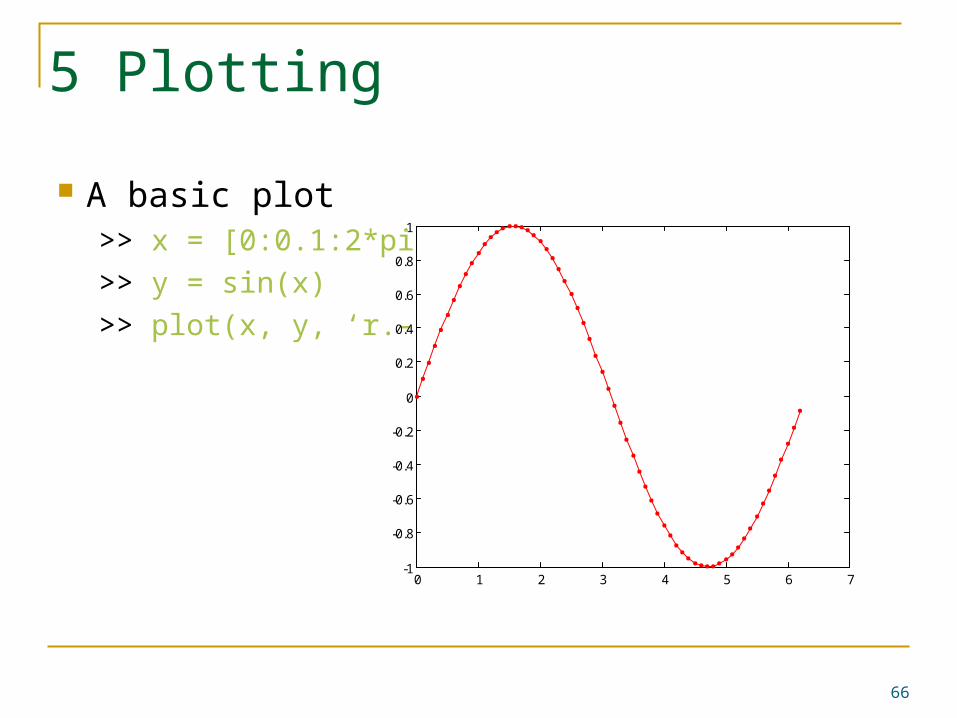
A basic plot>> x = [0:0.1:2*pi]

>> y = sin(x)

>> plot(x, y, ‘r.-’)

66

0 1 2 3 4 5 6 7-1

-0.8

-0.6

-0.4

-0.2

0

0.2

0.4

0.6

0.8

1

5 Plotting

Plotting a matrix MATLAB will treat each column as a different set of data

67

1 2 3 4 5 6 7 8 9 100.1

0.2

0.3

0.4

0.5

0.6

0.7

0.8

0.9

5 Plotting

Some other functions that are helpful to create plots:

hold on and hold off title legend axis xlabel ylabel

68

5 Plotting

>> x = [0:0.1:2*pi];>> y = sin(x);

>> plot(x, y, 'b*-')

>> hold on

>> plot(x, y*2, ‘r.-')

>> title('Sin Plots');

>> legend('sin(x)', '2*sin(x)');

>> axis([0 6.2 -2 2])

>> xlabel(‘x’);

>> ylabel(‘y’);

>> hold off

69

0 1 2 3 4 5 6-2

-1.5

-1

-0.5

0

0.5

1

1.5

2Sin Plots

x

y

sin(x)

2*sin(x)

5 Plotting

Plotting data

>> results = rand(10, 3)>> plot(results, 'b*')>> hold on>> plot(mean(results, 2), ‘r.-’)

70

1 2 3 4 5 6 7 8 9 100.1

0.2

0.3

0.4

0.5

0.6

0.7

0.8

0.9

5 PlottingError bar plot

>> errorbar(mean(data, 2), std(data, [], 2))

71

0 2 4 6 8 10 120.1

0.2

0.3

0.4

0.5

0.6

0.7

0.8

0.9

1Mean test results with error bars

5 Plotting

You can close all the current plots using ‘close all’

72

6 Save & load

73