introduction to measurement using oscilloscope

8/8/2019 Introduction to Measurement Using Oscilloscope

http://slidepdf.com/reader/full/introduction-to-measurement-using-oscilloscope 1/11

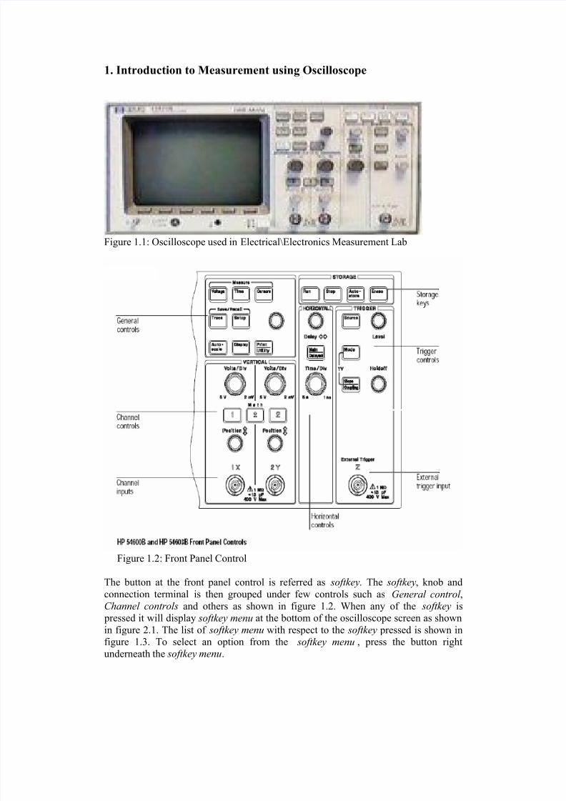
1. Introduction to Measurement using Oscilloscope

Figure 1.1: Oscilloscope used in Electrical\Electronics Measurement Lab

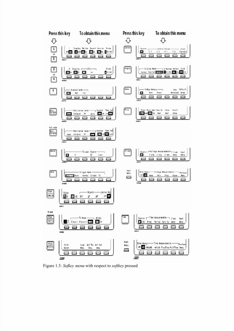
Figure 1.2: Front Panel Control

The button at the front panel control is referred as softkey. The softkey, knob and

connection terminal is then grouped under few controls such as General control ,Channel controls and others as shown in figure 1.2. When any of the softkey is

pressed it will display softkey menu at the bottom of the oscilloscope screen as shown

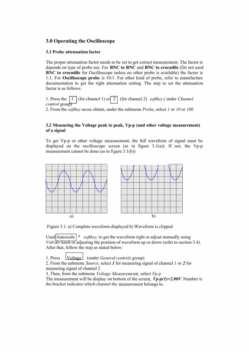
in figure 2.1. The list of softkey menu with respect to the softkey pressed is shown in

figure 1.3. To select an option from the softkey menu , press the button right

underneath the softkey menu.



Figure 1.3: Sofkey menu with respect to softkey pressed



2. Screen of Oscilloscope

Figure 2.1 below shows the information displayed on the Oscilloscope screen.

Figure 2.1: Information displayed at oscilloscope screen

Volt/div – value of the boxes on the oscilloscope screen vertically. The value can bechange using the knob labelled as Volt/div (at Channel control group)

Time/div - value of the boxes on the oscilloscope screen horizontally The

value can be change using the knob labelled as Time/div (at Horizontal control group)

1 2V 2 1V 0.00s 500us RUN

1

2

Source Voltage Measurement Clear Next

1 2 Vp-p Vavg Vrms Meas Menu

Volt/div or sensitivity for

channel 1

Volt/div or sensitivity for

channel 2

Time/div or sweep time

for all channels

Ground\zero reference of

channel 1

Ground\zero reference of

channel 2

0V reference of the

screen.

Softkey Menu

Volt/div

Time/div

submenu



3.0 Operating the Oscilloscope

3.1 Probe attenuation factor

The proper attenuation factor needs to be set to get correct measurement. The factor isdepends on type of probe use. For BNC to BNC and BNC to crocodile (Do not used

BNC to crocodile for Oscilloscope unless no other probe is available) the factor is

1:1. For Oscilloscope probe is 10:1. For other kind of probe, refer to manufacture

documentation to get the right attenuation setting. The step to set the attenuation

factor is as follows:

1. Press the 1 (for channel 1) or 2 (for channel 2) softkey ( under Channel control group)

2. From the softkey menu obtain, under the submenu Probe, select 1 or 10 or 100

3.2 Measuring the Voltage peak to peak, Vp-p (and other voltage measurement)

of a signal

To get Vp-p or other voltage measurement, the full waveform of signal must be

displayed on the oscilloscope screen (as in figure 3.1(a)). If not, the Vp-p

measurement cannot be done (as in figure 3.1(b))

a) b)

Figure 3.1: a) Complete waveform displayed b) Waveform is clipped

Used Autoscale * softkey, to get the waveform right or adjust manually using

Volt/div knob or adjusting the position of waveform up or down (refer to section 3.4).

After that, follow the step as stated below:

1. Press Voltage (under General controls group)

2. From the submenu Source, select 1 for measuring signal of channel 1 or 2 for

measuring signal of channel 2

3. Then, from the submenu Voltage Measurements, select Vp-p

The measurement will be display on bottom of the screen, Vp-p(1)=2.00V . Number is

the bracket indicates which channel the measurement belongs to.



3.3 Measuring the Frequency of a signal

To get frequency measurement, the full waveform must be displayed (as in voltage

measurement) and must be at least one complete cycle (as in figure 3.2(a)). If not,

the measurement can’t be done.

a) b)

Figure 3.2: a) Full waveform with more than one complete cycle b) waveform is not

one complete cycle

Used Autoscale * softkey, to get the waveform right or adjust manually using

Time/div knob. After that, follow step stated below:

1. Press Time sofkey (under General control group)

2. From the submenu Source, select 1 for measuring signal of channel 1 or 2 for

measuring signal of channel 2

3. Then, from the submenu Time Measurements, select Freq

The measurement will be display on bottom of the screen, Freq(1)=1.01kHz . Number

is the bracket indicates which channel the measurement belongs to* Autoscale will not work for waveform that has frequency 50Hz and below ( Refer to

section 4 for hint to display waveform manually)

3.4 Select Coupling

Step to select Coupling as follows:

1. Press the 1 (for channel 1) or 2 (for channel 2) softkey ( under Channel

control group)

2. From the softkey menu obtain, under the submenu Coupling, select DC or AC or for Ground Coupling

3.5 Adjust or moving the Ground/zero reference of a signal

To move the ground/zero reference of channel 1 or 2, use the knob label as Position(under the Channel control group) When, the knob is turned, there will be a display at the bottom left of the screen

showing the reading of Position ( ). To make the ground/zero reference centres to 0V reference of the screen, make sure that the Position ( ) reading is 0.00V.



3.6 Save waveform and display the saved waveform

3.6.1 Save a waveform

1. Press Trace sofkey (under General control group)

2. From the submenu Trace, select Mem1 to save inside memory 1 or select Mem2 to

save inside memory 2.3. Select Save to Mem, from the softkey menu.

3.6.2 Display the saved waveform

1. Press Trace sofkey (under General control group)

2. From the submenu Trace, select Mem1 to display waveform inside memory 1 or

select Mem2 to display waveform inside memory 2

3. From the submenu Trace Mem, select On. The waveform displayed from memory

will look a bit dimmer compared to original waveform. If the display need to be turn

off, then select Off from the submenu Trace Mem.

3.7 Phase Measurement, Time Delay and Lissajous using Cursor

3.7.1 Time Delay Method

1. Obtain two stable waveform on the oscilloscope screen

Figure 3.3: Two waveforms

2. Choose AC coupling for both channels

3. Move both waveform’s ground/zero reference to centred at 0V reference of the screen (Refer section 3.5)

Position (1) =0.00V a) Position (2) =0.00V b)

Figure 3.4: a) Channel 1 waveform centred b) Channel 2 waveform centred

1

2

1

2

1 2



4. To measure phase of waveform channel 2 relative to channel 1, identify the

positive peak of channel 2. Then, identify the positive peak of waveform of

channel 1 which is nearest toward right of waveform 2. (Figure 3.5).

Figure 3.5: Identifying the two peaks

5. Follow the two peaks downward until it intersects the 0V reference of the screen (Figure 3.6).

Figure 3.6: Identifying the two intersection points

6. Use cursor to measure the time (∆t) between these two intersection points.

Steps to use cursor as follow:

a. Press Cursor softkey (under General Controls group)

b. From submenu Active cursor, select t1. Move t1 cursor by using the knob under

the Cursor softkey until it ‘touch’ one of the intersection point. Then, select t2.

Move t2 to the next intersection point. Then, the ∆t reading can be obtained.

Substitute ∆t in suitable formula to get phase (Figure 3.7).

1 2

+ve peak of

channel 2

+ve peak of

channel 1

+ve peak of

channel 2

Nearest +ve peak of channel 1 toward right of

+ve peak of channel 2

+ve peak of

channel 2

Nearest +ve peak of

channel 1 toward right of

+ve peak of channel 2

Two

intersection

points

0V reference of the screen



t1= 1.01us t2=2.01us ∆t=1us

Figure 3.7: Placing cursor and getting ∆t value

3.7.2 Lissajous pattern phase measurement method

1. Follow step 1 until 3 of Time Delay Method

2. Press Main/Delayed softkey. ( under Horizontrol Control group)

3. Under submenu Horizontal Mode , select XY. The Lissajous pattern should be

obtain as in figure 3.8

Figure 3.8: Placing cursor on top and bottom

4. Press Cursor softkey. Set the Y2 cursor to the top of the signal, and set Y1 to the

bottom of the signal. ∆Y is the 2B (refer 2B in lab manual) value (refer to figure 3.8)

5. Then, place Y2 cursor to the top Y-axis intersection and Y1 cursor to the bottom Y-

axis intersection.(refer figure 3.9). ∆Y is the 2A value. Substitute both value (2B and

2A) in suitable formula to obtain the phase.

Figure 3.9: Y-axis intersections

t1 cursor t2 cursor

Y2

Y1

Y2

Y1

The Y-axis intersections

t1 cursor t2 cursor



4.0 Display wave properly using manual setting

Referring to previous section, it has been understood that the Autoscale function

won’t work on a waveform that has frequency less than 50Hz. It that case, manually

adjustment is needed. One way of doing it is by trial an error method, where we play

around with Volt/div and Time/div until we get the proper display. Another more

efficient way to do it is by estimating the required Volt/div and Time/div from thewaveform values.

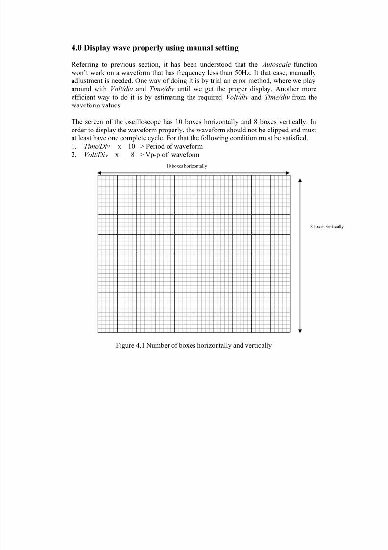
The screen of the oscilloscope has 10 boxes horizontally and 8 boxes vertically. In

order to display the waveform properly, the waveform should not be clipped and must

at least have one complete cycle. For that the following condition must be satisfied.

1. Time/Div x 10 > Period of waveform

2. Volt/Div x 8 > Vp-p of waveform

Figure 4.1 Number of boxes horizontally and vertically

10 boxes horizontally

8 boxes vertically



By using these two conditions, the Time/Div and Volt/div required can be estimated

For example, a sine wave with 8Vp-p and 20Hz need to be displayed on the

oscilloscope.

The minimum Time/Div required can be determined as follows:

Period of the waveform = Hz 20

1= 0.05s or 50ms

Time/div must be >10

50ms

Time/div must be > 10ms, adjusting Time/div to value slightly bigger, for example

20ms, will allow more than one cycle of waveform to be displayed

The minimum Volt/div required can be determined as follows:

Volt/div must be >8

8 pVp −

Volt/div must be > 1V, adjusting Volt/div to value slightly bigger, for example 2V,

will confirm the waveform is not clipped (assuming the waveform is centred)

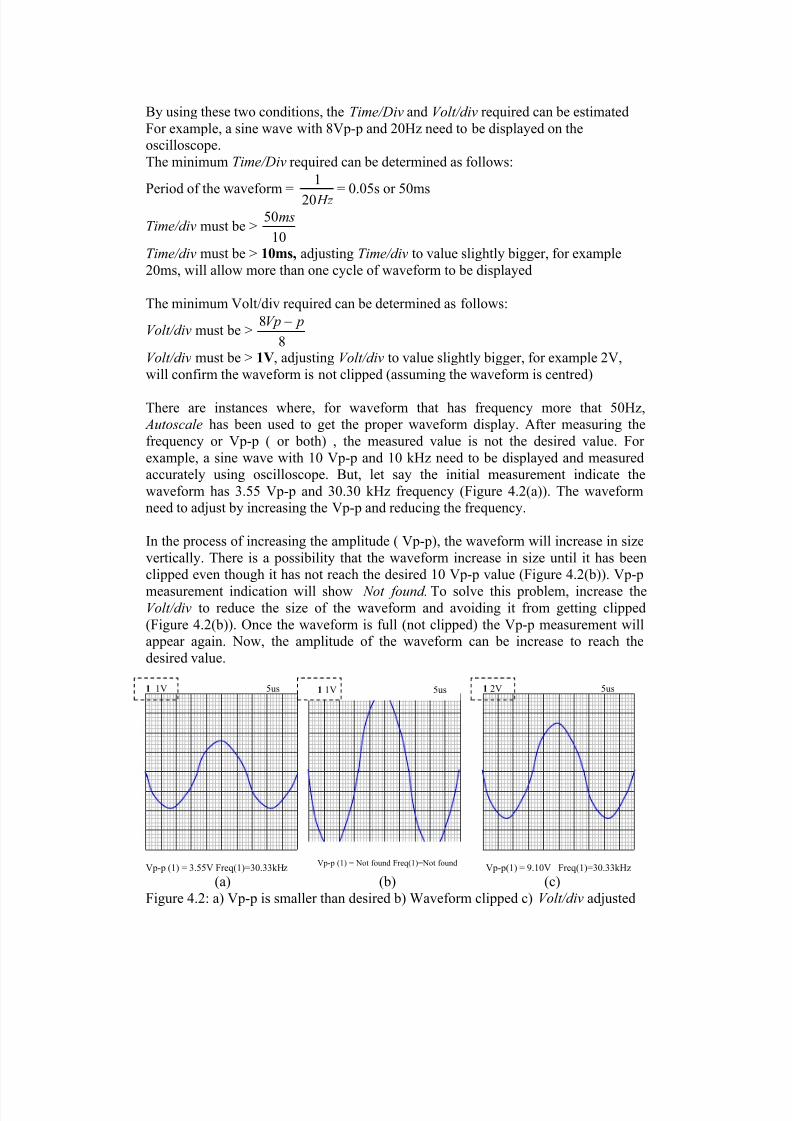
There are instances where, for waveform that has frequency more that 50Hz,

Autoscale has been used to get the proper waveform display. After measuring the

frequency or Vp-p ( or both) , the measured value is not the desired value. For

example, a sine wave with 10 Vp-p and 10 kHz need to be displayed and measured

accurately using oscilloscope. But, let say the initial measurement indicate the

waveform has 3.55 Vp-p and 30.30 kHz frequency (Figure 4.2(a)). The waveform

need to adjust by increasing the Vp-p and reducing the frequency.

In the process of increasing the amplitude ( Vp-p), the waveform will increase in size

vertically. There is a possibility that the waveform increase in size until it has been

clipped even though it has not reach the desired 10 Vp-p value (Figure 4.2(b)). Vp-p

measurement indication will show Not found. To solve this problem, increase theVolt/div to reduce the size of the waveform and avoiding it from getting clipped

(Figure 4.2(b)). Once the waveform is full (not clipped) the Vp-p measurement will

appear again. Now, the amplitude of the waveform can be increase to reach the

desired value.

1 1V 5us 1 2V 5us

Vp-p (1) = 3.55V Freq(1)=30.33kHz Vp-p(1) = 9.10V Freq(1)=30.33kHz

(a) (b) (c)

Figure 4.2: a) Vp-p is smaller than desired b) Waveform clipped c) Volt/div adjusted

Vp-p (1) = Not found Freq(1)=Not found

1 1V 5us



On the other hand, in the process of reducing the frequency, the period of the

waveform will increase (f =T

1), thus the size will increase horizontally. There is a

possibility that the waveform increase in size until it is has not more than one

complete cycle, even though it has not reach the desired 10 kHz value (Figure 4.3(b)).

Frequency measurement indication will show Not found. To solve this problem,

increase the Time/div to reduce the size of the waveform until it has more than onecomplete cycle (Figure 4.3(c)). Once the waveform is more than one complete cycle,

the Frequency measurement will appear again. Now, the frequency of the waveform

can be increase to reach the desired value.

1 1V 5us 1 1V 5us 1 1V 20us

Vp-p (1) = 3.55V Freq(1)=30.33kHz Vp-p (1) = 3.55V Freq(1)=Not found Vp-p (1) = 3.55V Freq(1)=18.18kHz

(a) (b) (c)

Figure 4.3: a) Freq. is bigger than desired b) Waveform is less then one complete

cycle c) Time/div adjusted

introduction to measurement using oscilloscope

Documents