introduction to mechanistic data-driven methods for ... · data exist in multiple length scales for...

Introduction to mechanistic data-driven methods for engineering, mechanical science and mechanics of

materials: difficulties in purely data-driven approaches for machine learning and some possible remedies

Prof. Wing Kam Liu, Walter P. Murphy Professor Director of Global Center on Advanced Material Systems and Simulation (https://camsim.northwestern.edu/)

Northwestern University, w‐[email protected]

Students, PostdocsHengyang Li Mahsa TajdariSatyajit MojumderSourav SahaPuikei ChengOrion L KafkaJiaying Gao Cheng YuDr. Zhengtao Gan

CollaboratorsGreg Olson (NU, QuesTek)NIST (Lyle Levine, Paul Witherell, Yan Lu)CHiMaD (https://chimad.northwestern.edu/)Jian Cao, Kori EhmannGreg WagnerCT Wu, Zeliang Liu, and John Hallquist (LSTC)Xianghui Xiao and Tao Sun (ANL)John Sarwark (Feinberg NU, Lurie Hospital)

1. Motivation: sources of data in mechanical science and engineering2. Mechanistic Machine Learning (MML) for mechanical science and

engineering– Interpretation of the data– Relevant concepts in data science– Introduction to different Machine Learning (ML) methods

a. Unsupervised learning b. Supervised learning

3. Applications of ML methods1. Topology optimization

1. Feed Forward Neural Network (FFNN)2. FFNN+ Convolutional Neural Network (CNN)

2. Adolescent Idiopathic Scoliosis1. FFNN2. Physics Guided Neural Network (PGNN)

4. Why we need reduced order models/methods (ROM)5. Summary and conclusions 6. References

Outline

© Northwestern Univ. 2019, 1

1. Motivation: source of data in mechanical science and engineering2. Mechanistic Machine Learning (MML) for mechanical science and







Outline


Multimodal data generation and collection

DATA

Information from sensors

Testdata

2D/3D/4Dimages

Model-based analysis

Strain Gauge[1]

Temperature sensing in Additive Manufacturing (AM)[2]

Measuring bone mineral density

AM exampleComposite structure

Pressure on intervertebral disc[3]

Extraction of data points from X-ray

Composite materials simulation

Composite coupon

CourtesyOf

NIST

Spine simulation

Fatigue life

AM Process simulation© Northwestern Univ. 2019, 3

Data generation and collection in composite systems

Woven composite

10.2 mm

Fiber diameter: 7 μm

84 μm

UD composite

[1] https://www.mhi.com/products/air/boeing_787.html

[1]

~60m

MoS2 reinforced polymer matrix

1 μm

Single lap bolt joint

Anomaly detection for fiber orientation

Experimental characterization and imaging

Interface fracture

Health monitoring for structural performance

Courtesy of AFRL

Courtesy of AFRL

Heterogeneous, non-stationary microstructure

Data exist in multiple length scales for composite materials system

Microstructure, material properties, structural performance. Information from four different scales are integrated to predict properties at part scale.

MoS2

Matrix

Courtesy of AFRL

• The following sample cases are based on Unidirectional (UD) composite microstructure • Local and average response of UD composite's Representative Volume Element (RVE) are of interest


Approach: experiments and modeling motivated by data

Validation by experiments

Data driven Process-structure-properties modeling

Mushy zone at melt pool

boundary

P520 S0.3

P416 S0.6

P520 S0.6

P520 S0.9

P520 S1.2

Imaging datasets

Keyhole morphology

Porosity structure

Cellular automaton (CA) modeling

Grain-scale thermal-mechanical modeling

Fatigue life

Scaling law discovery via machine learning Image-based fatigue predictions

(Cannot be observed by in-situ experiments)


*XR: Xray ** CT: Computerized Tomography, ***MR: Magnetic Resonance, courtesy: Lurie Children’s Hospital of Chicago

Data generation and collection in Adolescent Idiopathic Scoliosis (AIS)









Outline


Interpretation of data in mechanical science and engineering

DATA

Data analysis using Machine

Learning

Feature Engineering

Extraction of fiber dimension and fiber distribution from UD cross section

To extract meaningful data

Dimension Reduction

To reduce degrees of freedom

600 x 600 voxels

4 clusters

Reduced Order ModelsTo speed up the

computationInteraction tensor

To discover hidden relationships

Regression

Neural Network generated material

laws

To categorize data Classification

No debondingDebonding

Knowledge for applicationse.g. material systems design and discovery

Means Goals









Outline


Three types of machine learning in mechanical science and engineering

Machine Learning

Unsupervised Learning: self-organized data

pattern recognition

Supervised Learning:

mapping an input to an

output

Reinforcement Learning

Clustering: grouping objects

Dimension reduction:

reduces the number of features

Regression:Hidden

relationship between variables

Classification:Identifying

objects based on their class

Predicts microstructure averaged stress given external loading

Damage detection by stress contour

Data from: Li, H., Kafka, O. L., Gao, J., Yu, C., Nie, Y., Zhang, L., Tajdari, M., Tang, S., Guo, X., Li, G., Tang, S., Cheng, G., & Liu, W. K. (2019). Clustering discretization methods for generation of material performance databases in machine learning and design optimization. Computational Mechanics, 1-25.

e.g., Principal Component Analysis (PCA)

No damage

Damage

Unidirectional compositeStrain contour



Data-science is the “fourth paradigm” of science(empirical, theoretical, computational, data-driven) [21]

Data-Science: Transduction

Theory

Training data Test data

DeductionInduction

Transduction

Machine/Deep learning:Transduction: learn from given data to apply to new data [22]

Conventional methodsInduction: specific observations to general theory (bottom-up)Deduction: general theory to testable observations (top-down)

Relevant concepts in data science

Dimensionality Feature dimensionality: The number of features for each data point Input dimensionality: The total number of data points

Fidelity Quality of faithfulness of data

Fidelity

High LowLimited availability

High accuracy Relatively inexpensive

Multi‐fidelity

Low accuracy


A program or system that builds (trains) a predictive model from input dataMachine Learning

Relevant concepts in data science (cont)

A collection of rows or dataset with one or more features.Database


Feature engineering Process of determining which featuresmight be useful and converting

raw data into said features.

Individual independent variables defining characteristics of a data set. Informative and non‐redundant data.

Features

Dimension reduction Process of decreasing the number of dimensions representing a feature.

Objective function The mathematical formula or metric that a model aims to optimize.

Courtesy: Google developers https://developers.google.com/machine‐learning/glossary/#m

Illustration of relevant concepts for AIS*

Data gathered using 2D XR images

Source

Database Generation

Features Data points1 2 3 . . Ns

Xσ . . . . . .α . . . . . .t . . . . . .Δt

BMD

Features

High• Co‐ordinates from x‐ray• Age, test frequency

Low

Dimensionality of data( Ns): 17x2x6

Dimen

siona

lity of fe

atures

High

• Spinal angles• Stress

AgeCo‐ordinatesSpinal Angle

Stress BMD

Fidelity

*Adolescent Idiopathic Scoliosis

Spinal Angles Co‐ordinate BMD**

**Bone Mineral Density

X = Vector of input coordinates of a landmark [𝑋 𝑋 𝑋 ]

σ = Stress vector [σ11 σ22 σ33 σ12 σ23 σ31]

α = Global angel (Spinal Angles) vector [𝛼 𝛼 𝛼 𝛼 𝛼 ]

t = Age of the patient

Δt = age variance between target age and current age (month)

# vertebras# landmarks


Basic concepts of artificial neural network (ANN)

𝑊 : weights connecting neurons

Input layer Hidden layer

𝑎

Layer 𝑙 1 Layer 𝑙 2 Layer 𝑙 3

Output layer

𝑖

𝑎

𝑎

𝑎 𝑎

𝑊

𝑊

𝑊

𝑊

𝑊

𝑊

𝑎 : value of each neuron

Objective: To learn hidden relationship between input and output

𝑏 : bias on each neuron

Optimization problem: 𝑚𝑖𝑛𝑖𝑚𝑖𝑧𝑒 𝐸𝑟𝑟𝑜𝑟: 𝐸

12 𝜎∗ 𝑎 𝜎∗: 𝑡𝑎𝑟𝑔𝑒𝑡 𝑣𝑎𝑙𝑢𝑒

∆𝑊 𝛼𝛿𝑎



∆𝑊 𝛼𝛿𝑊 𝑎



Gradient descent[1] :

Assume 𝜎∗ 20

[1] Boyd, S., & Vandenberghe, L. (2004). Convex optimization. Cambridge university press.

𝜺 𝝈 (MPa)

Data point 1 0.1 20

Data point 2 0.2 38.6

…

𝛼: 𝑙𝑒𝑎𝑟𝑛𝑖𝑛𝑔 𝑟𝑎𝑡𝑒𝛿= 𝜎∗ 𝑎 )

Sample input data


Example of training Neural Network (NN): learning back-propagation

Neural network:

𝑎 𝑓 𝑊 , 𝑎

e.g. ReLU function,

Hidden layer

𝑎

Layer 𝑙 2 Layer 𝑙 3

Output layer

𝑎

𝑎

𝑎

𝑊

𝑊

𝑊

𝑏

Input layer

Layer 𝑙 1

𝜺𝜺 …

𝑎𝝈𝝈 …

Start training from data point 1


Check error, and iterate for convergence

𝐸𝑟𝑟𝑜𝑟: 𝐸12 𝜎∗ 𝑎

𝐸 4.5 → 0.5202

𝑖

𝑗𝑘

5.3

10.12

20.12

10.15

4.3

4.6

0.1

0.53

1.012

2.012

18.98 ∗

𝑊

The error will reduce by iteration, finally

𝐸 𝐸∗, 𝑐𝑜𝑛𝑣𝑒𝑟𝑔𝑒𝑛𝑐𝑒

Repeat for all data points until error is minimized


We often use a linear interpolation function 𝑓 𝑥 to approximate any continuous function 𝑓 𝑥 .

Goal function 𝑓 𝑥 :e.g. 𝑓 𝑥 exp 𝑥 0.5 /16 (blue line)

Approximate function: 𝑁 Nodes e.g. ∑ 𝑓 𝑥 𝑁 𝑥; 𝑥 , 𝑥 , 𝑥 , … , 𝑥 10, 5, 0, 4, 10(Orange line)

𝑓 𝑥

𝑥 𝑥𝑥

𝑓 𝑥

𝑥 𝑥𝑥

Neural Network as interpolation function[1]

[1] Zhang, L., Yang, Y., Li H., Gao J., Reno D., Tang S., Liu W.K. Neural network finite element method, in preparation[2] Approximation by superpositions of a sigmoidal function, by George Cybenko (1989).[3] Multilayer feedforward networks are universal approximators, by Kurt Hornik, Maxwell Stinchcombe, and Halbert White (1989).

Assume linear shape function


𝑓 𝑥 𝑁 𝑥; 𝑥 𝑇 𝑥; 𝑅𝑒𝐿𝑈, 𝑥 , 𝑥 , 𝑥 𝒇 𝒙𝑱

⟺ 𝐺 𝑥; 𝒘 𝑱, 𝒃 𝑱Shape function approximated by NN[2, 3]

𝑅𝑒𝐿𝑈: Rectified linear unit, usually in form: max 0, 𝑋

Unpublished results

Proof: NN for 1D shape function approximation

Lemma 1 The continuous piece‐wise linear function

can be represented by neural network as

𝑅𝑒𝐿𝑈 𝑅𝑒𝐿𝑈 𝑥 𝑎 𝑏 𝑎 𝑏 𝑎

e.g. a=‐1, b=0

Step 1: 𝑅𝑒𝐿𝑈 𝑥 1 1 Step 2: 𝑅𝑒𝐿𝑈 𝑅𝑒𝐿𝑈 𝑥 1 1 1

𝑎 𝑏

Zhang, L., Yang, Y., Li H., Gao J., Reno D., Tang S., Liu W.K. Neural network finite element method, in preparation

© Northwestern Univ. 2019, 23Unpublished results

x 𝑇

𝑏 =1

𝑊 , =1

𝑊 , =1

Output Layer(Layer 4)

Layer 2 Layer 3Input Layer（Layer 1）

𝑏 =1

Step 3: 𝑅𝑒𝐿𝑈 𝑅𝑒𝐿𝑈 𝑥 1Reflection: right part

Step 4: 𝑅𝑒𝐿𝑈 𝑅𝑒𝐿𝑈 𝑥 1 1 1𝑅𝑒𝐿𝑈 𝑅𝑒𝐿𝑈 𝑥 1

Combination: basis function

𝑊 , =‐1

𝑏 =1

𝑏 =0

𝑊 , =−1

𝑊 , = 1𝑏 1

𝑊 , =1

Proof: NN for 1D shape function approximation For 1D linear basis function, take the reflection to construct the right part and then combine these two parts.


x

𝑾𝒊 𝟏,𝒋 𝟏𝒍 𝟑

𝒃𝒋 𝟏𝒍 𝟐

𝒃𝒋 𝟐𝒍 𝟐

𝑾𝒊 𝟐,𝒋 𝟏𝒍 𝟑

𝑇

𝑏 =1

𝑊 ,

𝑏

𝑊 , =1

𝑊 , =‐1

Output Layer(Layer 4)

Layer 2 Layer 3Input Layer（Layer 1）

𝑊 ,

𝑏 =1

Effect of weights and biases on the output

Change in bias 𝒃𝒋𝒍 𝟐, changes the location Change in weights 𝑾𝒊 𝟏,𝒋

𝒍 𝟑 , changes the slopeZhang, L., Yang, Y., Li H., Gao J., Reno D., Tang S., Liu W.K. Neural network finite element method , in preparation

𝑿 𝑻

Data point 1 1 0

Data point 2 0.5 0.3

…









Outline


A simple illustration on unsupervised learning for clustering

1 2 3 4

2 4 6 8

6 8 2 4

4 6 8 6

2 4 0 2

Four individual data points

Five Features

Clustering(e.g., K‐means clustering)

1.5 3.5

3 7

7 3

5 7

3 1

Clustering: Reduces the data dimensionality

Cluster 1 Cluster 2

Averaged two columns

Objective: Group 4 data points (each having five features) into 2 clusters

Two clusters


How does K‐means clustering work ?

𝑨 𝐴 , 𝐴 … 𝐴

𝑀 data points 𝑨

…

Raw data

𝑺 , k=1

𝐾clusters

𝑁 dimensional

Average points 𝑾

𝑘: index of clusters𝑚: index of data points

𝑚𝑖𝑛𝑖𝑚𝑖𝑧𝑒: 𝑨 𝑾𝑨 ∈ 𝑺

𝑺 , k=2

𝑺 , k=3Data point 𝑨

𝑺 , k=4

𝑺 , k=5

𝑺 , k=6

Mathematically:

𝑨 ：Data point in cluster 𝑺𝑾 ：Average point in cluster 𝑺

：Euclidean distance

Cluster: Points with most similar values Has one average point: mean average of nearby data

points Objective:

Minimize total distance between each average point andthe data points within its cluster.

Concept of K-means Clustering

Watt, J., Borhani, R., & Katsaggelos, A. K. (2016).Machine learning refined: foundations, algorithms, and applications. Cambridge University Press. © Northwestern Univ. 2019, 28

32

25

20

15

10

51

Strain distribution Cluster distribution based on strain intensity

Grouping local material points in the microstructure based on strain responses (or other quantities, such as effective plastic strain)

K-means clustering for Unidirectional (UD) composite

2D microstructure with 600 by 600 voxels

2D microstructure with 32 clusters

The strain field, originally represented by 360,000 voxels, is now represented by 32 clusters

The strain patterns are adequately captured by the clusters


Self-Organizing Map (SOM) - Concept

Cluster: Points with most similar values Has one average point: weighted average of nearby data points

Objective:Distribute all data points into a map of 𝑲𝟏 𝑲𝟐 clusters so that the dissimilarity within a cluster is minimized, and the dissimilarity between clusters with nearby indexes is minimized

How does Self-Organizing Map work? [12,13]

𝑨 𝐴 , 𝐴 … 𝐴

𝑀 data points 𝑨

…

Raw data

𝑁 dimensional

Average points 𝑾

Data point 𝑨

𝐾 𝐾 clusters

3 2

𝑚𝑖𝑛𝑖𝑚𝑖𝑧𝑒: ℎ ||𝑘 𝑘′||,

,

𝑨 𝑾𝑨 ∈ 𝑺

,

,

||𝑘 𝑘′||: Euclidean distance between clusters’ indexesℎ ||𝑘 𝑘′|| : Gaussian kernel function


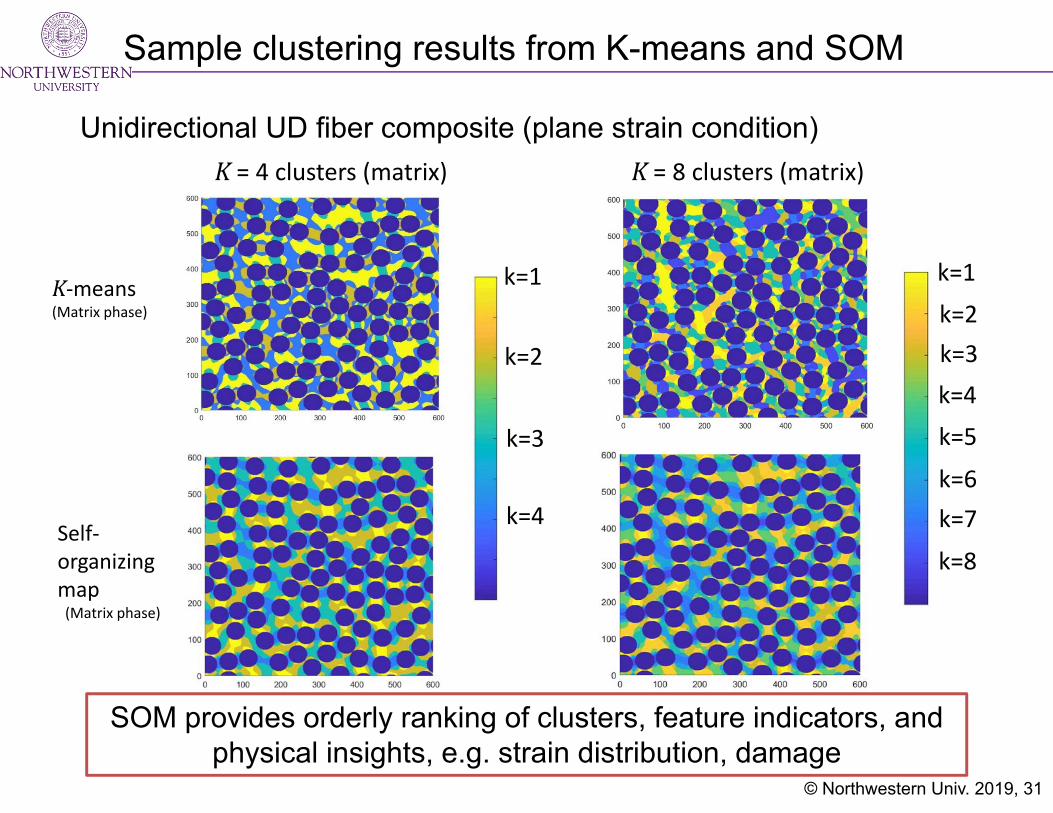
Unidirectional UD fiber composite (plane strain condition)

K‐means(Matrix phase)

Self‐organizing map(Matrix phase)

Sample clustering results from K-means and SOM

k=1

k=2

k=3

k=4

k=1

k=2k=3

k=4

k=6

k=5

k=7

k=8

SOM provides orderly ranking of clusters, feature indicators, and physical insights, e.g. strain distribution, damage


K= 8 clusters (matrix)K= 4 clusters (matrix)

Supervised learning

Supervised learning establishes the hidden relationship between the input and output data.

Courtesy: http://aiobserve.com/AI/ML/31.html

Data Training Prediction

Quick overview of Supervised Learning

Can predict the material law from input and output strain‐stress data.

Used for – Regression and Classification

σ = NN(ε)

Sample [1] experimentTraining Prediction

[1] Tang, S., Zhang, G., Yang, H., Guo, X., Li, Y., & Liu, W. K. (2019). MAP123: A Data-driven Approach to Use 1D Data for 3D Nonlinear Elastic Materials Modeling, CMAME (Submitted) © Northwestern Univ. 2019, 32

Regression

Regression: prediction of response to an input based on a prioriknowledge of the relationship between input and output data.

𝜎 𝑣𝑠 𝜀

𝝈 𝑓 𝜺 (hypothesis)

𝜺 𝝈.. ..

.. ..

Input Data1,2

1. Gather data from experiment or high-fidelity microstructure numerical simulation2. Assume plain strain. 𝜺 and 𝝈each contain three components

Li, H, Kafka, OL, Gao, J, Yu, C, Nie, Y, Zhang, L, Tajdari, M, Tang, S, Guo, X, Li, G, Tang, S, Cheng, G & Liu, WK 2019, Clustering discretization methods for generation of material performance databases in machine learning and design optimization, Computational Mechanics. https://doi.org/10.1007/s00466-019-01716-0

Find a relationship between stress and straine.g. 𝜎 2 ∗ 𝜀 1

Hypothesis: linear or nonlinear relationship


Regression using Feed Forward Neural Network (FFNN)

The relationship between input and output can be explored usingFFNN (an ANN with multiple hidden layers)

𝜺 𝝈.. ..

.. ..

Input Data1,2



FFNN training: solving the following optimization problem

Regression using Convolutional Neural Network (CNN) for inverse modeling

For a microstructure with given micro-stress distribution, can CNN predict the macro-strain?Micro‐stress xx distribution

Micro−stress yy distribution

Micro‐stress xy distributionUnidirectional microstructure

What is the macro-strain ?

Inverse modeling

𝜀

𝜀

𝛾


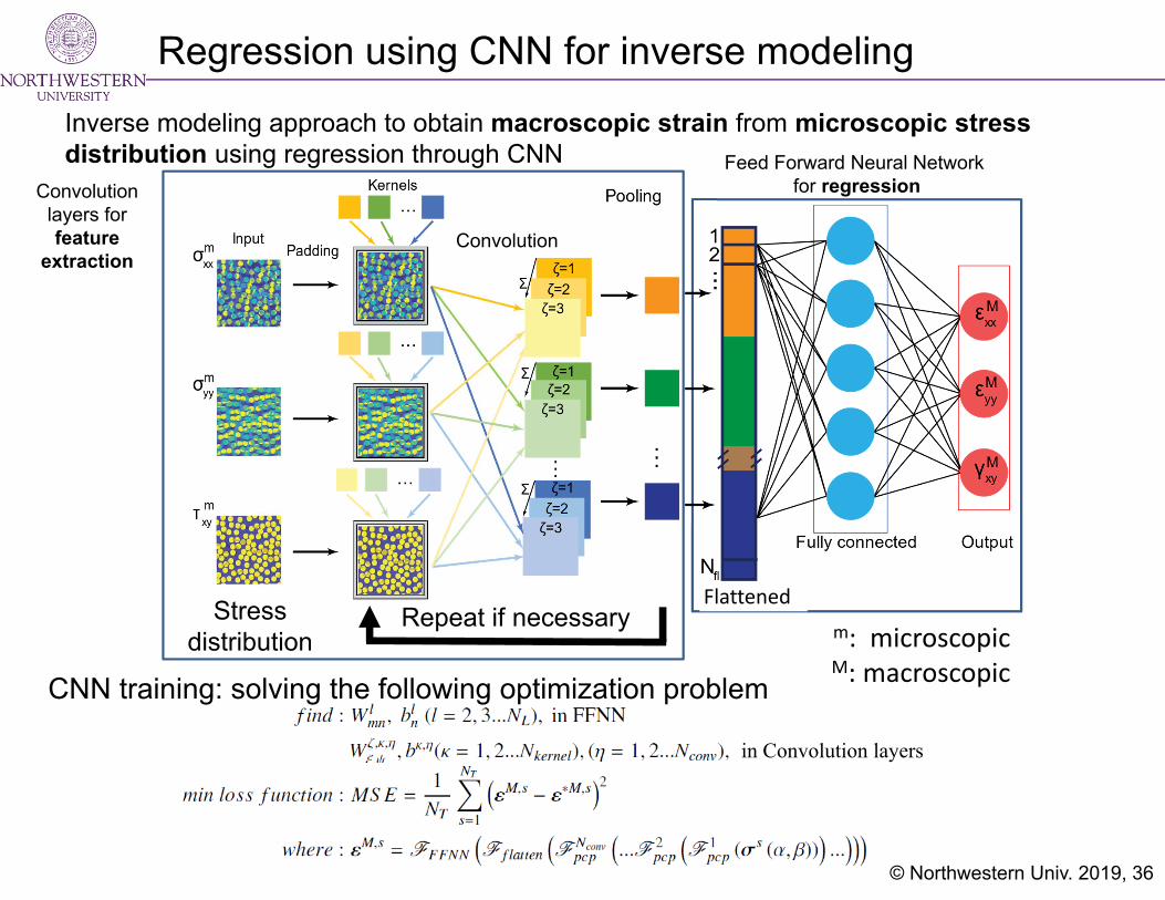
Inverse modeling approach to obtain macroscopic strain from microscopic stress distribution using regression through CNN

Regression using CNN for inverse modeling


Stress distribution

Feed Forward Neural Network for regression

Flattened

Convolution

Repeat if necessary

CNN training: solving the following optimization problem

in Convolution layers

Convolution layers forfeature

extraction

m: microscopicM: macroscopic

Classification of damage Classification is a process of predicting the known class of given data

points.

E.g., classify the state of the microstructure as “no damage” or “damage” based on local stress distribution

No damage Damage



• Microscale material point damage is defined as: for any material point in the microscale domain, if the micro-stress exceeds certain threshold, the micro material point is damaged

• Macroscale material point damage is defined as:1) PD > PND, damage in the microstructure2) PD < PND, no damage in the microstructure *P is probability

Macroscale

Microscale

Microscale

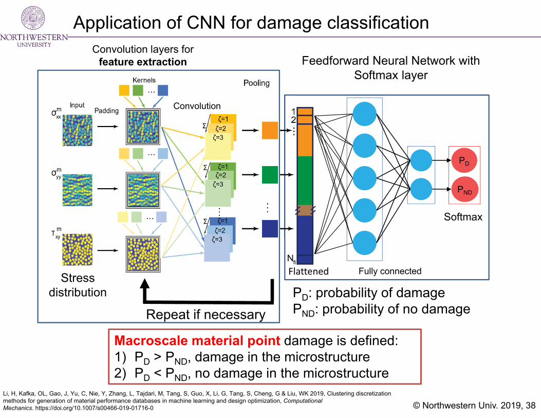
Application of CNN for damage classification

Stress distribution

Feedforward Neural Network with Softmax layer

Flattened

Convolution

Repeat if necessary

Fully connected

Softmax

PD

PND

Macroscale material point damage is defined:1) PD > PND, damage in the microstructure2) PD < PND, no damage in the microstructure

PD: probability of damagePND: probability of no damage


Convolution layers forfeature extraction









Outline



Car frame[1]

6m

Multiple length scales composite systems design & Optimization

[1]https://www.cgtrader.com/3d‐models/vehicle/part/car‐frame‐03[2]https://www.comsol.com/blogs/performing‐topology‐optimization‐with‐the‐density‐method/

30cm

Part[2]

Name Part Woven composite

UD composite

MoS2 polymer Total

Length scale cm mm μm μm -Number of mesh 10,000 40,000 36,0000 90,000 1.296×1019

Multiscale Design: Topology

𝐿ayer angle: 𝛼

𝑊𝑜𝑣𝑒𝑛 𝑡ℎ𝑖𝑐𝑘𝑛𝑒𝑠𝑠: ℎ 𝐹𝑖𝑏𝑒𝑟 𝑟𝑎𝑑𝑖𝑢𝑠: 𝑟

𝐹𝑖𝑏𝑒𝑟 𝑣𝑜𝑙𝑢𝑚𝑒 𝑓𝑟𝑎𝑐𝑡𝑖𝑜𝑛: 𝑉

𝐷𝑒𝑛𝑠𝑖𝑡𝑦 𝑑𝑖𝑡𝑟𝑖𝑏𝑢𝑡𝑖𝑜𝑛：𝜌 𝑥

𝑀𝑜𝑆 𝑣𝑜𝑙𝑢𝑚𝑒 𝑓𝑟𝑎𝑐𝑡𝑖𝑜𝑛: 𝑉

Woven composite

10.2 mm

84 μm

UDfiber composite

1 μm

Nanoscale reinforced

polymer matrix

Approximate optimization iterations

200 200 200 100 ‐

Total calculation cost ‐ ‐ ‐ ‐ A tremendous

number

Number of elements 360.000

Topology optimization (TopOpt)


Design region Applied external loading

[1] Sigmund, O. (2001). A 99 line topology optimization code written in Matlab. Structural and multidisciplinary optimization, 21(2), 120-127.

Minimizing system compliance

60 cm

30 c

m

• Homogenous material assumed• No microstructure• Only elastic responses considered

Design region

60 cm

30 c

m

𝜀

𝜀

𝛾

𝜺 𝝈

Single-scale topology optimization

[1]

Microstructure-based topology optimization is a two-scale problem

Two-scale TopOpt:• Microstructures in all material points • Design of microstructures and structure

topology- Evaluation of microstructure is time consuming during design iterations- Can FFNN and CNN approximate microstructure responses efficiently and accurately?

Applied external loading

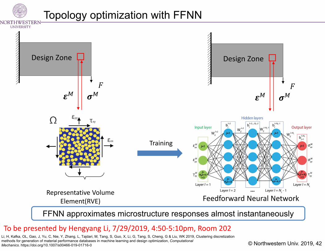
Topology optimization with FFNN


FFNN approximates microstructure responses almost instantaneously

𝐹𝝈𝜺

Design Zone

Representative Volume Element(RVE) Feedforward Neural Network

𝐹𝝈𝜺

Design Zone

Training

To be presented by Hengyang Li, 7/29/2019, 4:50‐5:10pm, Room 202 Li, H, Kafka, OL, Gao, J, Yu, C, Nie, Y, Zhang, L, Tajdari, M, Tang, S, Guo, X, Li, G, Tang, S, Cheng, G & Liu, WK 2019, Clustering discretization methods for generation of material performance databases in machine learning and design optimization, Computational Mechanics. https://doi.org/10.1007/s00466-019-01716-0

TopOpt with FFNN for nonlinear elastic materials


𝜎 𝐶 𝜀

Linear elastic response

𝐹

𝝈

𝜺Design Zone

Optimization

𝜎 ℱ 𝜀

Optimization

𝐹

𝝈

𝜺Design Zone

Nonlinear RVE response predicted by FFNN

Linear material Nonlinear FEM-FEM two scale Nonlinear FEM-FFNN two scale

Initial compliance 𝑁 · 𝑐𝑚 295.0 ‐ 375.0

Optimized compliance 𝑁 · 𝑐𝑚 28.0 ‐ 38.0

Optimization calculation time 𝑠 338 𝟐𝟐𝟎 𝟏𝟎𝟔 472

Factor of speed‐up over FE‐FE ‐ ‐ 280,255FEM: finite element methodLi, H, Kafka, OL, Gao, J, Yu, C, Nie, Y, Zhang, L, Tajdari, M, Tang, S, Guo, X, Li, G, Tang, S, Cheng, G & Liu, WK 2019, Clustering

discretization methods for generation of material performance databases in machine learning and design optimization, Computational Mechanics. https://doi.org/10.1007/s00466-019-01716-0

TopOpt with FFNN+CNN for nonlinear elastic materials with damage constraints


Linear material Nonlinear FEM‐FEM two scale Nonlinear FEM‐(FFNN+CNN) two scale

Initial compliance 𝑁 · 𝑐𝑚 295.0 ‐ 295

Optimized compliance 𝑁 · 𝑐𝑚 30 ‐ 31

Optimization calculation time 𝑠 12.6 𝟔𝟔𝟎 𝟏𝟎𝟔 14.5

Factor of speed‐up over FE‐FE ‐ ‐ 𝟒𝟓 𝟏𝟎𝟔

FEM: finite element method

Optimization with linear elastic material

Optimization with FFNN+CNN









Outline


Data-driven approach in predicting Adolescent Idiopathic Scoliosis (AIS)

FeaturesData points (l)

1 2 3 . . NsXα . . . . . .t . . . . . .ΔtX*

X = Vector of input coordinates of a landmark [𝑋 𝑋 𝑋 ]α = Global angle vector [𝛼 𝛼 𝛼 𝛼 𝛼 ]t = Age of the patient.Δt = age variance between target age and current age (month).X* = Vector of output co-ordinates of a landmark 𝑋∗ 𝑋∗ 𝑋∗].Ns = Total number of landmarks = 2x6x17 = 204

Spinal global angles

6 Landmarks

6 Landmarks

2x6

# vertebras

Using all features to train the Neural

Network for all I=1,..,Ns

x 17

© Northwestern Univ. 2019, 46To be presented by Mahsa Tajdari, 7/31/2019, 2:40-3:00pm, Room 208

Physics Guided Neural Network (PGNN) to predict patient specific constants

© W.K. Liu Group, Northwestern University 47

Assume linear relationship between effective stress and growth rate 𝑋 between time m∆𝑡 and n∆𝑡

𝑋 m n A 1 B 𝜎𝜎 : effective stress at time n∆𝑡∆𝑡 : unit of time (month)

𝐀 𝑚𝑜𝑛𝑡ℎ and 𝑩 𝑀𝑃𝑎 are patient specific constants that are calibrated inside the NN

Calculating Hyper Parameters in NN

Landmark𝜎

ℱ

𝜎

Spine FE M

odel

𝜎𝑀𝑆𝐸𝑿∗, MSE 𝑀𝑆𝐸 𝑀𝑆𝐸

MSE MSE 𝑿∗, 𝑿∗,

MSE MSE 𝑋 m n 𝑨𝑻𝑯 1 𝑩𝑻𝑯 𝜎

MSE MSE 𝑋 m n 𝑨𝐋𝐔 1 𝑩𝐋𝐔 𝜎Hyper parameters (𝑨𝑻𝑯, 𝑩𝑻𝑯, 𝑨𝐋𝐔, 𝑩𝐋𝐔 ) will be calculate inside NN

𝑋∗,

𝑋∗,

𝑋∗,

X‐ray 2D images

Generate patient specific model

Mean Square Error (MSE) corresponding ℱ

𝐀𝑻𝑯 𝑚𝑜𝑛𝑡ℎ and 𝑩𝑻𝑯 𝑀𝑃𝑎 patient specific constants for Thoracic vertebrae𝐀𝑳𝑼 𝑚𝑜𝑛𝑡ℎ and 𝑩𝑳𝑼 𝑀𝑃𝑎 patient specific constants for Lumbar vertebrae


Composite NN using Multi-fidelity dataSp

ine FE M

odel

Physical data based FFNN Data based FFNN

m n 𝑨𝑻𝑯 1 𝑩𝑻𝑯 𝜎 𝑋 0

m n 𝑨𝐋𝐔 1 𝑩𝐋𝐔 𝜎 𝑋 0

𝑿 : position of data point in 𝑚 month𝑿 : position of data point in 𝑛 month

α = Global angle vector [𝛼 𝛼 𝛼 𝛼 𝛼 ]

t = Age of the patient.

Δt = age variance between target age and current age (month).

X* = Vector of output co-ordinates of a landmark 𝑋∗ 𝑋∗ 𝑋∗]

Relative Error Data based FFNN: 18.5%

PGNN: 4.63%

Physical Equation

Raw Data

FFNN

PGNN








Outline


Multiscale design and optimization is not feasible with direct microstructure responses calculation with Finite Element Method (FEM)

Well-trained NNs accelerates microstructure and structure design process, e.g. Topology Optimization

Material microstructure responses database is required for the training process.

The database includes: Macro-strain and macro-stress pairs Micro-stress distribution and macro-strain pairs Other microstructure quantities of interest

Rich database of mechanical response information are necessary for training various Neural Networks


The gap:Microstructure response simulation can be expensive

using FEM Rich database requires a lot of runs of microstructure

simulation

Cost of microstructure responses database generation

𝜺 𝜀 , 𝜀 , 𝛾 𝑛 1,2 … , 1000

1,000 load cases for training a 2D hyper elastic problem:

𝝈 𝜎 , 𝜎 , 𝜏 𝑛 1,2 … , 1000

Microscopic stressExternal loading states Averaged stress

Li, H, Kafka, OL, Gao, J, Yu, C, Nie, Y, Zhang, L, Tajdari, M, Tang, S, Guo, X, Li, G, Tang, S, Cheng, G & Liu, WK 2019, 'Clustering discretization methods for generation of material performance databases in machine learning and design optimization', Computational Mechanics. https://doi.org/10.1007/s00466-019-01716-0 © Northwestern Univ. 2019, 51

𝜀

𝜀𝛾

𝜏

𝜎𝜎

600 x 600 x 3 x 1000

𝜎

𝜎

𝜏

Running 1,000 microstructure simulation is expensive:

Microstructure simulation method Total simulation time (s)

FFT 3.01 x 105

FEM 2.04 x 107

HPC is needed

Approximate material responses using FFNN

How to generate microstructure responses efficiently?

𝜺 𝜀 , 𝜀 , 𝛾 𝑛 1,2 … , 1000

𝝈 𝜎 , 𝜎 , 𝜏 𝑛 1,2 … , 1000

External loading states Averaged stress

Li, H, Kafka, OL, Gao, J, Yu, C, Nie, Y, Zhang, L, Tajdari, M, Tang, S, Guo, X, Li, G, Tang, S, Cheng, G & Liu, WK 2019, 'Clustering discretization methods for generation of material performance databases in machine learning and design optimization', Computational Mechanics. https://doi.org/10.1007/s00466-019-01716-0

Data point Feature

1 𝜺𝟏

2 𝜺𝟐

…

n 𝜺𝒏

Data point Feature

1 𝝈𝟏

2 𝝈𝟐

…

n 𝝈𝒏


FFNN with well-trained parameters

Curse of dimensionality in complex material systems

1.38x1025

1.38x1025

Woven composite

10.2 mm Fiber diameter: 7 μm

84 μmUD composite

1 μm

MoS2 reinforced polymerSingle lap bolt joint

36x106

10 clusters

64x103

10 clusters

2x106

96 clusters

1x106

𝐊 𝐊 … 𝐊𝐊 𝐊 … 𝐊

⋮𝐊

⋮𝐊

⋱ ⋮… 𝐊

𝛿𝐝𝛿𝐝

⋮𝛿𝐝

𝐫𝐫

⋮𝐫

DoFs using FEM: 3 𝑁 𝑁 𝑁 ⋯ 𝑁 𝑁 𝑁 𝑁

Strong interaction between scales

Number of elements using FEM: 1x10 ∗2.6x10 ∗36x10 ∗64x10 =6x10𝟐𝟓elements

Extremely large problem

𝑁 : number of integration points𝑁 : number of nodesSuperscripts indicate scale level

𝐌 𝐌 … 𝐌𝐌 𝐌 … 𝐌

⋮𝐌

⋮𝐌

⋱ ⋮… 𝐌

𝛿𝛆𝛿𝛆

⋮𝛿𝛆

𝐫𝐫

⋮𝐫

DoFs using MCA: 6 𝑁 ⋯ 𝑁 𝑁 𝑁 𝑁 𝑁 : number of clusters

𝑁 ≪ 𝑁 at each scale

10 clusters

Number of clusters using MCA: 10 * 96 * 10 *10 = 9.6x104 clusters

Solvable on small HPC/single PC

639420

639420


Material Scale:

Typical number of elements:

Clusters used:

FEM MCA

Two-scale theory: Self-consistent Clustering Analysis (SCA) overview

• Objective: Efficient and accurate homogenization of nonlinear history dependent heterogeneous materials with complex microstructure.

Self‐consistent Clustering Analysis (SCA)

Data‐driven order reduction Group points in the MVE that are mechanically similar

Mechanistic prediction

• Lippmann‐Schwinger integral equation

• Micromechanics mean‐field theory

1. Liu, Z., Bessa, M. A., & Liu, W. K. (2016). Computer Methods in Applied Mechanics and Engineering

2. Liu, Z., Fleming, M., & Liu, W. K. (2018). Computer Methods in Applied Mechanics and Engineering

3. Bessa, M. A., Bostanabad, R., Liu, Z., Hu, A., Apley, D. W., Brinson, C., ... & Liu, W. K. (2017). Computer Methods in Applied Mechanics and Engineering

4. Liu, Z., Kafka, O. L., Yu, C., & Liu, W. K. (2018). In Advances in Computational Plasticity

5. Tang, S., Zhang, L., & Liu, W. K. (2018). Computational Mechanics6. Kafka, O. L., Yu, C., Shakoor, M., Liu, Z., Wagner, G. J., & Liu, W. K. (2018). JOM7. Shakoor, M., Kafka, O. L., Yu, C., & Liu, W. K. (2018). Computational Mechanics8. Li, H., Kafka, O. L., Gao, J., Yu, C., Nie, Y., Zhang, L., ... & Tang, S. (2019). Computational Mechanics

9. Zhang, L., Tang, S., Yu, C., Zhu, X., & Liu, W. K. (2019). Computational Mechanics10. Gao, J., Shakoor, M., Jinnai, H., Kadowaki, H. Seta, E., Liu. W. K. An Inverse Modeling Approach for Predicting Filled Rubber Performance. (2019) Computer Methods in Applied Mechanics and Engineering

Numerical verification

System Complexity Computational time Speed-up

FEM 80x80x80 25.7 hr (24 cores) 1ROM (SCA)

16256

2 s50 s

1x106

5x104

FEM Model Reduced Order Model (ROM)

To be covered in Lecture 2© Northwestern Univ. 2019, 54

Material design requires a large database of microstructure response information

Reduced order modeling (ROM) allows fast data generation for: Different heterogeneous microstructures Different material constituents

Why use reduced order modeling for data generation?

ROM, 8 clustersROM, 16 clustersDNS (5 % error bar)

RVE Stress, M

Pa

RVE Strain

Fiber phase (2 clusters)

Matrix phase (8 clusters)

y

zxApply loading in

y direction

DNS: ~200 hr using 80 cpusROM: 2 s using 1 cpu

The microstructure database generation can now be done on single PC


Rich datasets provide us an opportunity to integrate mechanical anddata sciences for rapid prediction, design, and optimization.

Data science enables solution of large-scale problems, otherwise nottractable using current methodologies.

Reduce Order Models (ROM) such as Principal Component Analysis(PCA), Self-consistent Clustering Analysis (SCA), MultiresolutionClustering Analysis (MCA), help us rapidly generate key datasets.

Machine learning techniques such as neural networks (FFNN, CNN,PGNN, etc.) can augment ROMs for extremely fast computations.

Combining ROMs with machine learning techniques has the potentialto discover, design, and optimize novel complex material systems.

Mathematical theories for biological systems are in their infancy;discovery of hypotheses in biological system might be achieved byconsidering physics, e.g. via a physic guided neural network

Conclusions



Acknowledgement

Funding agencies:• Air Force Office of Scientific Research• Army Research Office• Beijing Institute of Collaborative Innovation• Bridgestone Corporation• DMDII (UI Labs)• Ford Motor Company/National Energy

Technology Laboratory• Lurie Children’s Hospital• NIST CHiMaD I and CHiMaD II• NIST Gaithersburg• Northwestern University Data Science

Initiative• NSF

• GRFP DGE-1324585• CMMI MOMS• CMMI CPS

Our thanks to…

References

[1] Li, H., Kafka, O. L., Gao, J., Yu, C., Nie, Y., Zhang, L., Tajdari, M., Tang, S., Guo, X., Li, G., Tang, S., Cheng, G., & Liu, W. K. (2019). Clustering discretization methods for generation of material performance databases in machine learning and design optimization. Computational Mechanics[2] Boyd, S., & Vandenberghe, L. (2004). Convex optimization. Cambridge university press.[3] Zhang, L., Yang, Y., Li H., Gao J., Reno D., Tang S., Liu W.K. Neural network finite element method, in preparation[4] Approximation by superpositions of a sigmoidal function, by George Cybenko (1989)[5] Multilayer feedforward networks are universal approximators, by Kurt Hornik, Maxwell Stinchcombe, and Halbert White (1989).[6] Zhang, L., Yang, Y., Li H., Gao J., Reno D., Tang S., Liu W.K. Neural network finite element method, in preparation[7] Watt, J., Borhani, R., & Katsaggelos, A. K. (2016).Machine learning refined: foundations, algorithms, and applications. Cambridge University Press.[8] Tang, S., Zhang, G., Yang, H., Guo, X., Li, Y., & Liu, W. K. (2019). MAP123: A Data-driven Approach to Use 1D Data for 3DNonlinear Elastic Materials Modeling, Computer Methods in Applied Mechanics and Engineering (Submitted)[9] Sigmund, O. A 99 line topology optimization code written in Matlab. (2001). Structural and multidisciplinary optimization[10] Liu, Z., Bessa, M. A., & Liu, W. K. (2016). Computer Methods in Applied Mechanics and Engineering[11] Liu, Z., Fleming, M., & Liu, W. K. (2018). Computer Methods in Applied Mechanics and Engineering[12] Bessa, M. A., Bostanabad, R., Liu, Z., Hu, A., Apley, D. W., Brinson, C., ... & Liu, W. K. (2017). Computer Methods in Applied Mechanics and Engineering[13] Liu, Z., Kafka, O. L., Yu, C., & Liu, W. K. (2018). In Advances in Computational Plasticity[14] Tang, S., Zhang, L., & Liu, W. K. (2018). Computational Mechanics[15] Kafka, O. L., Yu, C., Shakoor, M., Liu, Z., Wagner, G. J., & Liu, W. K. (2018). JOM[16] Shakoor, M., Kafka, O. L., Yu, C., & Liu, W. K. (2018). Computational Mechanics[17] Li, H., Kafka, O. L., Gao, J., Yu, C., Nie, Y., Zhang, L., ... & Tang, S. (2019). Computational Mechanics[18] Zhang, L., Tang, S., Yu, C., Zhu, X., & Liu, W. K. (2019). Computational Mechanics[19] Gao, J., Shakoor, M., Jinnai, H., Kadowaki, H. Seta, E., Liu. W. K. An Inverse Modeling Approach for Predicting Filled Rubber Performance. (2019) Computer Methods in Applied Mechanics and Engineering


introduction to mechanistic data-driven methods for ... · data exist in multiple length scales for...

Documents