introduction to modern nuclear physics
TRANSCRIPT

Introduction to Modern Nuclear Physics
Qun Wang
May 16, 2019

1
Department of Modern Physics, University of Science and Technology of China, Anhui 230026China, [email protected], http://sta.ustc.edu.cn/~qunwang

Contents
1 Introduction 5
1.1 Why nuclear physics . . . . . . . . . . . . . . . . . . . . . . . . . . . . . . . . . . . . . 51.2 From cgs-Gaussian to natural unit system . . . . . . . . . . . . . . . . . . . . . . . . . 51.3 Conventions . . . . . . . . . . . . . . . . . . . . . . . . . . . . . . . . . . . . . . . . . . 8
2 Properties of Nuclei 11
2.1 Discover atomic nucleus . . . . . . . . . . . . . . . . . . . . . . . . . . . . . . . . . . . 112.2 The size and density distribution of nucleus . . . . . . . . . . . . . . . . . . . . . . . . 122.3 Spin and magnetic moment . . . . . . . . . . . . . . . . . . . . . . . . . . . . . . . . . 132.4 Parity . . . . . . . . . . . . . . . . . . . . . . . . . . . . . . . . . . . . . . . . . . . . . 202.5 Electric multipole moment . . . . . . . . . . . . . . . . . . . . . . . . . . . . . . . . . . 212.6 The mass formula and binding energy . . . . . . . . . . . . . . . . . . . . . . . . . . . 23
3 Radioactivity and nuclear decay 28
3.1 General property of radioactivity . . . . . . . . . . . . . . . . . . . . . . . . . . . . . . 283.2 Radioactive dating . . . . . . . . . . . . . . . . . . . . . . . . . . . . . . . . . . . . . . 373.3 α decay: strong interaction at work . . . . . . . . . . . . . . . . . . . . . . . . . . . . . 383.4 β decay: weak interaction at work . . . . . . . . . . . . . . . . . . . . . . . . . . . . . 46
3.4.1 Fermi theory of β decay . . . . . . . . . . . . . . . . . . . . . . . . . . . . . . . 533.4.2 Parity violation in β decay . . . . . . . . . . . . . . . . . . . . . . . . . . . . . 65
3.5 γ decay: electromagnetic interaction at work . . . . . . . . . . . . . . . . . . . . . . . 663.5.1 Classical electrodynamics for radiation eld . . . . . . . . . . . . . . . . . . . . 663.5.2 Quantization of radiation eld . . . . . . . . . . . . . . . . . . . . . . . . . . . 693.5.3 Interaction of radiation with matter . . . . . . . . . . . . . . . . . . . . . . . . 713.5.4 Multipole expansion . . . . . . . . . . . . . . . . . . . . . . . . . . . . . . . . . 76
3.6 Mössbauer eect . . . . . . . . . . . . . . . . . . . . . . . . . . . . . . . . . . . . . . . 91
4 Nuclear models 93
4.1 The shell model . . . . . . . . . . . . . . . . . . . . . . . . . . . . . . . . . . . . . . . . 934.1.1 Phenomena related to shell structure . . . . . . . . . . . . . . . . . . . . . . . . 934.1.2 Main points of the shell model . . . . . . . . . . . . . . . . . . . . . . . . . . . 94
4.2 Collective models . . . . . . . . . . . . . . . . . . . . . . . . . . . . . . . . . . . . . . . 1014.3 Hatree-Fock self-consistent method . . . . . . . . . . . . . . . . . . . . . . . . . . . . . 103
5 Nuclear reaction 109
5.1 Conservation laws and kinematics . . . . . . . . . . . . . . . . . . . . . . . . . . . . . . 1105.2 Partial wave analysis and optical potential . . . . . . . . . . . . . . . . . . . . . . . . . 1135.3 Resonance and compound nuclear reaction . . . . . . . . . . . . . . . . . . . . . . . . . 1155.4 Direct reaction . . . . . . . . . . . . . . . . . . . . . . . . . . . . . . . . . . . . . . . . 1185.5 Nuclear ssion . . . . . . . . . . . . . . . . . . . . . . . . . . . . . . . . . . . . . . . . 119
5.5.1 Spontaneous ssion . . . . . . . . . . . . . . . . . . . . . . . . . . . . . . . . . . 119
2

CONTENTS 3
5.5.2 Induced ssion . . . . . . . . . . . . . . . . . . . . . . . . . . . . . . . . . . . . 1235.5.3 Self-sustaining nuclear ssions and ssion reactor . . . . . . . . . . . . . . . . . 1275.5.4 Time constant of a ssion reactor . . . . . . . . . . . . . . . . . . . . . . . . . . 128
5.6 Accelerator-Driven System . . . . . . . . . . . . . . . . . . . . . . . . . . . . . . . . . . 1295.6.1 Spallation neutron source . . . . . . . . . . . . . . . . . . . . . . . . . . . . . . 1295.6.2 Thorium as ssion fuel . . . . . . . . . . . . . . . . . . . . . . . . . . . . . . . . 1295.6.3 Nuclear waste incinerator . . . . . . . . . . . . . . . . . . . . . . . . . . . . . . 130
5.7 Nuclear fusion . . . . . . . . . . . . . . . . . . . . . . . . . . . . . . . . . . . . . . . . . 130
6 Nuclear force and nucleon-nucleon interaction 140
6.1 Properties of nucleons . . . . . . . . . . . . . . . . . . . . . . . . . . . . . . . . . . . . 1406.2 General properties of nuclear force . . . . . . . . . . . . . . . . . . . . . . . . . . . . . 1406.3 Deuteron nucleus . . . . . . . . . . . . . . . . . . . . . . . . . . . . . . . . . . . . . . . 145
6.3.1 S-state . . . . . . . . . . . . . . . . . . . . . . . . . . . . . . . . . . . . . . . . . 1456.3.2 S and D states . . . . . . . . . . . . . . . . . . . . . . . . . . . . . . . . . . . . 147
6.4 Low energy nucleon-nucleon scatterings . . . . . . . . . . . . . . . . . . . . . . . . . . 1516.5 Nucleon-Nucleon scatterings in moderate energy . . . . . . . . . . . . . . . . . . . . . 1526.6 Meson exchange model for NN potentials . . . . . . . . . . . . . . . . . . . . . . . . . 152
6.6.1 One pion exchange potential (OPEP) . . . . . . . . . . . . . . . . . . . . . . . 1536.6.2 One boson exchange potential . . . . . . . . . . . . . . . . . . . . . . . . . . . . 155
7 The structure of hadrons 161
7.1 Symmetries and Groups . . . . . . . . . . . . . . . . . . . . . . . . . . . . . . . . . . . 1617.1.1 The group SU(2) . . . . . . . . . . . . . . . . . . . . . . . . . . . . . . . . . . . 1647.1.2 SU(2) isospin, fundamental representation . . . . . . . . . . . . . . . . . . . . . 1667.1.3 Conjugate representation of SU(2) . . . . . . . . . . . . . . . . . . . . . . . . . 1677.1.4 SU(3) symmetry . . . . . . . . . . . . . . . . . . . . . . . . . . . . . . . . . . . 1687.1.5 Tensor representation of SU(3) . . . . . . . . . . . . . . . . . . . . . . . . . . . 1737.1.6 Reduction of direct product of irreducible representations in SU(3) . . . . . . . 1747.1.7 Quarks as building blocks for hadrons . . . . . . . . . . . . . . . . . . . . . . . 1757.1.8 Mesons as quark-anti-quark states . . . . . . . . . . . . . . . . . . . . . . . . . 1777.1.9 Baryons as three-quark states . . . . . . . . . . . . . . . . . . . . . . . . . . . . 1817.1.10 Gell-Mann-Okubo relations . . . . . . . . . . . . . . . . . . . . . . . . . . . . . 185
7.2 Quarks and gluons . . . . . . . . . . . . . . . . . . . . . . . . . . . . . . . . . . . . . . 1887.2.1 Color degrees of freedom . . . . . . . . . . . . . . . . . . . . . . . . . . . . . . . 1887.2.2 Gluons as color carriers . . . . . . . . . . . . . . . . . . . . . . . . . . . . . . . 1917.2.3 Asymptotic Freedom . . . . . . . . . . . . . . . . . . . . . . . . . . . . . . . . . 1947.2.4 Phenomenological illustration of the connement [7] . . . . . . . . . . . . . . . 196
8 Acknowledgement 200
A Nucleon-nucleon scattering theory 201
A.1 Nucleon-nucleon scatterings . . . . . . . . . . . . . . . . . . . . . . . . . . . . . . . . . 201A.2 The stationary scattering wave function . . . . . . . . . . . . . . . . . . . . . . . . . . 201A.3 Cross section . . . . . . . . . . . . . . . . . . . . . . . . . . . . . . . . . . . . . . . . . 202A.4 The optical theorem . . . . . . . . . . . . . . . . . . . . . . . . . . . . . . . . . . . . . 203A.5 Partial wave method . . . . . . . . . . . . . . . . . . . . . . . . . . . . . . . . . . . . . 204
A.5.1 Scattering amplitude and cross section . . . . . . . . . . . . . . . . . . . . . . . 205A.5.2 Inelastic scattering and total cross section . . . . . . . . . . . . . . . . . . . . 207A.5.3 Phase shifts in square well scattering . . . . . . . . . . . . . . . . . . . . . . . . 209A.5.4 Breit-Wigner formula . . . . . . . . . . . . . . . . . . . . . . . . . . . . . . . . 210
A.6 Scatterings of identical particles . . . . . . . . . . . . . . . . . . . . . . . . . . . . . . . 211

CONTENTS 4
A.7 Lippman-Schwinger equation and Green function method . . . . . . . . . . . . . . . . 212
B A: Bessel functions 216
C B: Spherical harmonic functions 220
D Solutions to problems 223

Chapter 1
Introduction
1.1 Why nuclear physics
Nuclear physics is one of the most important branches and milestones in modern physics in the lastcentury. It has intrinsic connections to quantum mechanics and can be regarded as a laboratory forquantum physics. The aim of nuclear physics is to understand the properties of nuclei and theirapplications. Among many applications are (a) The origin of nuclei in the universe, i.e. nuclearnucleosynthesis, nuclear cross section is the key to understanding of nuclear reaction in astrophysics;(b) Nuclear energy, nuclear ssion and fusion; (c) Nuclear transmutation of radioactive waste withneutrons; (d) Radiotherapy for cancer with proton and heavy ion beams; (e) Medical Imaging, suchas nuclear Magnetic Resonance Imaging (MRI), X-ray imaging with better detectors and lower doses,Positron-Electron Tomography (PET); (f) Radioactive Dating, such as C-14/C-12 dating for deadlives, Kr-81 dating for ground water; (g) Element analysis, such as forenesic (as in hair), biology(elements in blood cells) and archaeology (provenance via isotope ratios).
1.2 From cgs-Gaussian to natural unit system
We use natural units [~, c, eV] (the Planck constant, speed of light, and electro-Volt) for angularmomentum, velocity and energy to replace [g,cm,s] (gram, centmeter and second) for mass, lengthand time [1]. So any quantities in the cgs unit can be expressed as gacmbsc, and in the natural unitit can be expressed by ~αcβeVγ .
For electromagnetic phenomena, there are several unit system, here we will use cgs-Gaussianunits, in particular, the unrationalized Gaussian units (not Lorentz-Heaviside ones). We will explainit in more details. In dealing with thermal phenomena, we have an additional unit kB (Boltzmannconstant) in the natural unit or equivalently K (Kelvin) in the cgs unit. The relations between twosystems of units are given by
1 ~ = 1.05× 10⁻²⁷ g · cm2 · s−1
1 c = 2.99792458× 1010 cm · s−1 (1.1)
1 eV = 1.60217653× 10⁻¹² g · cm2 · s−2
1 kB = 1.3806488× 10⁻¹⁶g · cm2 · s−2 ·K−1 (1.2)
5

CHAPTER 1. INTRODUCTION 6
From the above we can get the inverse relation
1 cm = 5.06× 10⁴ ~ · eV−1 · c1 g = 5.6× 1032 eV · c−2
1 s = 1.52× 10¹⁵ ~ · eV−1
1 K = 8.617× 10⁻⁵ eV · k−1B (1.3)
Now we explain the feature of unrationalized Gaussian units in electromagnetics. In this unitsystem, the Maxwell equations are written as
∇ ·E = 4πρ,
∇×B =4π
cj +
1
c
∂E
∂t,
∇ ·B = 0,
∇×E = −1
c
∂B
∂t, (1.4)
where the electric and magnetic elds have the same unit. The inverse-square force laws are writtenas
F =q1q2
r3r,
F =1
c2
∫ ∫I1dl1 × (I2dl2 × r)
r3. (1.5)
We see that two of Maxwell equations (1.4) have the factor 4π while there is no such a factor in theforce laws. However in Lorentz-Heaviside units or rationalized Gaussian units, one can absorb 4π inMaxwell equations by redening elds and charges. As a price there are 4π factors in the force laws.The elds and charges in two unit systems are related by
ELH =1√4π
Eunrat−Gauss,
qLH =√
4πqunrat−Gauss. (1.6)
In nuclear physics, the unit for thermal system is not used very often. So we stick to the unit[~, c, eV] or [g,cm,s] for convenience. From the relations in Eq. (1.2) we can derive following usefulconversion factors
~c = 197 MeV · fme2 ≈ 1
137~c (1.7)
We have e2 ≈ 1/137 in unrationalized Gaussian units. In contrast this relation becomes e2/(4π) ≈1/137 in rationalized Gaussian or Lorentz-Heaviside units.
In the cgs-Gaussian units, the charge is in the electrostatic unit (esu) which can be determinedfrom the Coulomb law
F =q2
r3r→ esu2 = g · cm · s−2 × cm2 = g · cm3 · s−2
→ esu = g1/2 · cm3/2 · s−1 (1.8)
We know that the Coulomb force law in the SI system has the following form
F =1
4πε0
q2
r3r (1.9)

CHAPTER 1. INTRODUCTION 7
where ε0 = 8.8542 × 10⁻¹² C2N−1m−2 and the charge unit is Coulomb (C). We can determine theconversion rule for C to esu. In the SI system, we have q = 1 C and r = 1 m, then the force isF = 8.99 × 10⁹ N. In the unrationalized Gaussian units, we have q = 1 esu and r = 1 cm, then theforce is F = 1 dyn = 10−5 N. Comparing two units, we obtain 1 C = 3× 10⁹ esu. An electron carriesthe charge
1 e = 1.602× 10⁻¹⁹ C = 4.8× 10⁻¹⁰ esu (1.10)
In the SI system, the unit of the electric eld is Volt/m = N/C, while in the unrationalized Gaussianunits, the electric and magnetic elds have the same unit: Gauss (G). So we have
1 Gauss =dyn
esu= g1/2 · cm−1/2 · s−1
1 Volt = 1 N ·m/C =107 dyn · cm
3× 10⁹ esu
=1
3× 10⁻²esuVolt
esuVolt = g1/2 · cm1/2 · s−1 (1.11)
where we have the static Volt unit: esuVolt. Then we obtain 1 eV = 1.6 × 10⁻¹² g · cm2 · s−2, thethird line of Eq. (1.2). Also we obtain
e2 = 2.304× 10⁻¹⁹ esu2 = 2.304× 10⁻¹⁹ g · cm3 · s−2
~c = 3.15× 10⁻¹⁷ g · cm3 · s−2 (1.12)
which give the second line of Eq. (1.7). We can express ~c by
~c = 3.15× 10⁻¹⁷ (g · cm2 · s−2) · cm
= 3.15× 10⁻⁴(g · cm2 · s−2) · fm= 197 MeV · fm (1.13)
which is the rst line of Eq. (1.7).Now we can convert some quantities in natural units. For electric and magnetic elds in cgs units,
we have
1 Gauss = g1/2 · cm−1/2 · s−1
= 6.92× 10⁻² (~c)−3/2 · eV2 (1.14)
We can convert the proton and neutron masses in cgs unit to natural unit.
mp = 1.672622× 10⁻²⁴ g = 938.27208 MeV · c−2
mn = 1.674927× 10⁻²⁴ g = 939.56541 MeV · c−2 (1.15)
Atomic mass unit is dened as 1/12 of the mass of 126 C, i.e. N−1
A ·gram where NA = 6.022142× 10²³
is the Avogadro constant. Atomic unit is
1 u = 1.66× 10⁻²⁷ kg = 931.494 MeV/c2, (1.16)
The proton and neutron mass in the atomic mass unit are
mp = 1.007276 u
mn = 1.008665 u (1.17)
Here is an example involving another natural unit kB. The shear viscosity is dened by F = ηS dvdx andentropy density is dened as thermal energy sTΩ (Ω is the volume). Their dimensions are determinedfrom knowns,
[η] = g · cm−1 · s−1
[s] = cm−3 · kB (1.18)

CHAPTER 1. INTRODUCTION 8
So the ration η/s has the dimension
[η/s] = g · cm2 · s−1 · k−1B = ~ · k−1
B (1.19)
In this book we take the natural unit ~ = c = kB = 1. In summary, a quantity has the dimension[D] = gacmbsdKf = ~αcβeVγkδB, by using Eq. (1.2) and (1.3), we can obtain following relations
α = a+ d
β = a− 2b
γ = −a+ b− d+ f
δ = −f (1.20)
1.3 Conventions
We list conventions for notations as follows. All superscripts or subscripts standing for texts inmathematical expressions are shown in roman letters, those standing for variables are shown innormal mathematical mode.

CHAPTER 1. INTRODUCTION 9
Table 1.1: Conventions for notations.Symbols Physical QuantitiesJ, JA (1) Total angular momentum quantum number; (2) Nuclear spin quantum numberJ,JA (1) Total angular momentum; (2) Nuclear spinL Orbital angualr momentum quantum numberL Orbital angualr momentumM (1) Atomic mass of an element; (2) Quantum transition amplitude;
(3) Orbital angualr momentum quantum number along one particular directionS (1) Spin quantum number; (2) S-matrix; (3) S-factor in WKB approximation;
(4) Area in coordinate spacem (1) Nuclear mass; (2) Nucleon mass
x, r 3-dimensional coordinates space pointsx, r Modula of 3-dimensional coordinate space points, x = |x|, r = |r|xi, ri Three components of coordinates space points, i = 1, 2, 3R Nuclear radiusq Particle chargee Electric charge of a protonQ (1) Electric quadrupole; (2) Q-valueµ Magnetic momentg (1) g-factor in magnetic moment; (2) Coupling constant
k,p 3- dimensional momentumk, p Modula of 3-dimensional momentum, k = |k|, p = |p|A Nucleon number in a nucleusZ Proton number in a nucleusN (1) Neutron number in a nucleus; (2) Particle number;
(3) Quantum number in harmonic oscillatorn (1) Radial quantum number; (2) Occupation quantum number; (3) Particle numberE Electric eldB Magnetic eldA Electromagnetic vector potentialE EnergyB Binding energy

CHAPTER 1. INTRODUCTION 10
Exercise 1. Unit transformation. Shear viscosity is a measure of the resistance of a uidwhen it is deformed by shear stress, often denoted as η. Entropy density is the entropyper unit volume, denoted as s. Please try to express the unit of η/s in terms of ~ andkB, with ~=h/2π the reduced Planck constant, and kB the Boltzmann constant. [Note: InInternational System of Units, the unit of η is Pascal·Second.]
Exercise 2. Nuclear magneton. Convert the nuclear magneton in the natural unit µN = e2mp
to the unit of Hertz/Tesla, where e is the electric charge of the proton in unit of Coulomb,and mp is the proton mass.
Exercise 3. Given 1 Volt = esuVolt× 13 × 10−2, calculate e2/(~c).

Chapter 2
Properties of Nuclei
The static properties such as the charge, radius, spin, magnetic moment, electric qaudrapole etc. arebasic properties of nuclei. The dynamic properties include the structure and decay of nuclei.
2.1 Discover atomic nucleus
The beginning of particle and nuclear physics started from Rutherford's alpha scattering experiments,which was the rst experiment where a microscopic particle was shooted as projectiles into anothermicroscopic particle as target to detect the content of the target particle. This is the prototype ofmodern particle and nuclear physics experiments.
To quote Rutherford in his original paper, "By means of a diaphragm placed at D, a pencil ofalpha particles was directed normally on to the scattering foil F. By rotating the microscope [M] thealpha particles scattered in dierent directions could be observed on the screen S."
To quote Rutherford, "I had observed the scattering of alpha-particles, and Dr. Geiger in mylaboratory had examined it in detail. He found, in thin pieces of heavy metal, that the scatteringwas usually small, of the order of one degree. One day Geiger came to me and said, "Don't you thinkthat young Marsden, whom I am training in radioactive methods, ought to begin a small research?"Now I had thought that, too, so I said, " Why not let him see if any alpha-particles can be scatteredthrough a large angle?" I may tell you in condence that I did not believe that they would be, sincewe knew the alpha-particle was a very fast, massive particle with a great deal of energy, and youcould show that if the scattering was due to the accumulated eect of a number of small scatterings,the chance of an alpha-particle's being scattered backward was very small. Then I remember twoor three days later Geiger coming to me in great excitement and saying "We have been able to getsome of the alpha-particles coming backward . . . " It was quite the most incredible event that everhappened to me in my life. It was almost as incredible as if you red a 15-inch shell at a piece oftissue paper and it came back and hit you."
The Rutherford alpha scattering experiment proved that in the center of an atom locates its hardcore called nucleus with positive charge due to the large angle scatterings.
In 1932, Chadwick found neutron by bombarding Beryllium with α particles to produce Carbon-12, 4
2He+94Be→ 12
6 C+n. He was awarded the Nobel prize later in 1935 for this discovery. Heisenbergproposed that a nucleus is made of protons and neutrons. This marked the birth of nuclear physics.
A Nucleus is labeled by AZXN (in simple version, poeple also use A
ZX or AX), where X is thename of the nucleus, A is the number of proton and neutrons A = Z +N , with Z/N the number ofprotons/neutrons. A nuclide is the nucleus with specic proton and neutron number. Isotope is thenuclide with the same Z but dierent N , isotone is that with the same N but dierent Z. Isobar:the same A but dierent Z.
The nucleus mass can be measured by mass spectrometer. Often the material is heated to producean atomic vapor. Then the electron beam in transverse direction are used to strip the electrons out
11

CHAPTER 2. PROPERTIES OF NUCLEI 12
Figure 2.1: Rutherford alpha scattering experiments.
Source
Collimator
particleα
Thin Au foil
Detector
θ
of the atoms to make them ions. These ions are accelerated by an electric eld and then pass throughan area with a magnetic led exerted in upward direction perpendicular to the ion velocity. Theseions are then bent in a circular motion and some nally enter the detector, see Fig. 2.4. Those ionsthat pass through the magnetic zone to enter the detector satisfy qv|B| = mv2/R, where q, v,m,Rare the charge, circulating velocity, mass and radius of the circle the particle moves, respectively.Then we can get the mass from m = qR|B|/v.
The Segre chart is the chart for nuclides in Z versus N . For light nuclei, we have Z ∼ N , but forheavier nuclei, we have Z < N .
2.2 The size and density distribution of nucleus
A nucleus is a collection of protons and neutrons which can be regarded as a bulk of nuclear matter.If the nucleus is treated as a sphere, while the volume of a nucleus is proportional to the number ofnucleons A, then the radius of the nucleus is in the form,
R = r0A1/3, (r0 ≈ 1.2 fm) (2.1)
We can estimate the density of a nucleus. The number and mass densities are
n0 =A
V≈ A
(4/3)πr30A≈ 0.138 fm−3 ≈ 1.38× 1038 cm−3
ρ0 = nmN ≈ 2.3× 10¹⁴ g · cm−3 (2.2)
Actually it is not very precise to regard the nucleus as a sphere with a uniform density. The electronscatterings tell us that a nucleus does not have a rigorous boundary but a surface with the width of2-3 fm where the charge density gradually drops to zero. One can use the Woods-Saxon distribution(or the Fermi distribution) to discribe the nuclear charge density,
ρ(r) =ρ0
1 + exp[(r −R)/a](2.3)
where a ≈ 0.54 fm. The width of the surface t can be dened by the criterion that the density dropsfrom 90% to 10% of ρ0,
t ≈ 4.4a ≈ 2.4 fm (2.4)
One can introduce the angular dependence of the radius R(θ) to describe the non-spherical shapes ofthe nuclei,
R(θ) = R0[1 + β2Y20(θ) + β4Y40(θ) + · · · ] (2.5)

CHAPTER 2. PROPERTIES OF NUCLEI 13
Figure 2.2: Chadwick found neutrons. The unknown particles carry no charges and has almost thesame mass as proton.
Po
Source
Be9
α
neutron
C12
target nuclei (H,He,N,...)
neutron
recoil particle
where only even numbers l appear in spherical harmonic functions Yl0.
2.3 Spin and magnetic moment
Any microscopic particles have angular momenta. If they contain charged constituents they also havemagnetic moments. Here is the classical picture for magnetic moment. When a charged particle hasorbital angular momentum it must have a magnetic moment. Suppose it carries a charge q and movein a circle with radius r and velocity v. Then its angular momentum is L = mvr. The magneticmoment is the area times the current, µ = πr2 qv
2πr = q2mL.
Now let us consider the Maxwell equations (1.4) for magnetostatics,
∇×B = 4πj,
∇ ·B = 0. (2.6)
Using B = ∇×A, we obtain∇(∇ ·A)−∇2A = 4πj. (2.7)
We impose Coulomb gauge condition ∇ ·A = 0 and the above becomes
∇2A = −4πj, (2.8)
whose solution is
A(r) =
∫d3r′
j(r′)
|r− r′| (2.9)
We can make expansion of the integrand for r = |r| r′ = |r′|,1
|r− r′| =1
r− r′i ∂i
1
|r− r′|
∣∣∣∣r′=0
+ · · · = 1
r+ r′i
rir3
+ · · · (2.10)

CHAPTER 2. PROPERTIES OF NUCLEI 14
Figure 2.3: Chart of Nuclide [see, e.g. http://atom.kaeri.re.kr/ton/nuc8.html andhttp://nsspi.tamu.edu/media/878612/img1.jpg]

CHAPTER 2. PROPERTIES OF NUCLEI 15
Figure 2.4: Mass spectrometer.
Figure 2.5: The nuclear density distribution.
r (fm)
0 1 2 3 4 5 6 7 8 9 10
ρ
0
0.02
0.04
0.06
0.08
0.1
0.12
0.14
0.16
Pb208
Fe56

CHAPTER 2. PROPERTIES OF NUCLEI 16
Figure 2.6: Elastic electron scattering of the charge distribution of 16O, see Fig. 1(A) and Fig. 5 ofRef. [23].

CHAPTER 2. PROPERTIES OF NUCLEI 17
Then Eq. (2.9) becomes
A(r) =1
r
∫d3r′j(r′) +
rir3
∫d3r′r′ij(r
′) + · · ·
=rir3
∫d3r′r′ij(r
′) + · · · (2.11)
where the rst term is vanishing∫d3r′j(r′) = 0. This can be shown by using ∇ · j = 0 and
0 =
∫d3r′∇′ · (r′ij) =
∫d3r′(ji + r′i∇′ · j)
=
∫d3r′ji (2.12)
We can also have the following identity for j,
0 =
∫d3r′∇′ · (r′ir′kj) =
∫d3r′(r′kji + r′ijk + r′ir
′k∇′ · j)
=
∫d3r′(r′kji + r′ijk) (2.13)
Then we can re-write Eq. (2.11) as
A(r) = −ekri
2r3
∫d3r′[r′kji(r
′)− r′ijk(r′)]
= −ek1
2r3εkilri
∫d3r′[r′ × j(r′)]l
= − 1
r3r× µ (2.14)
where the magnetic moment is dened by
µ =1
2
∫d3r′r′ × j(r′) (2.15)
If we consider a system of charged particles, the current density is given by
j(r) =∑i
qiviδ(r− ri) (2.16)
where ri and vi are position and velocity of the particle i. Then the magnetic moment in Eq. (2.15)can be re-written as
µ =1
2m
∑i
qi
∫d3r′(r′ × pi)δ(r
′ − ri)
=1
2m
∑i
qiLi (2.17)
where Li = ri × pi is the oribital angluar momentum for the particle i.The quantum origin of the magnetic moment can be seen as follows. When a charged particle is
placed in an external magnetic eld, its kinetic energy term is modied to
p2
2m→ (p− qA)2
2m→ (−i∇− qA)2
2m
→ iq(∇ ·A + A · ∇)
2m=iq
mA · ∇
= − iq
2m(r×B) · ∇ =
iq
2mB · (r×∇)
= − q
2mB · L, (2.18)

CHAPTER 2. PROPERTIES OF NUCLEI 18
where the vector potential A is related to the constant magnetic eld B by
A = −1
2r×B (2.19)
One can verify
(∇×A)k = −1
2εijk∂i(r×B)j = −1
2εijkεlsj∂i(rlBs)
=1
2(δilδks − δisδkl)Bs∂irl
=1
2Bk∂iri −
1
2Bi∂irk = Bk
∇ ·A = ∂iAi = −1
2εijkBk∂irj = 0 (2.20)
One can dene the orbital magnetic moment from Eq. (2.18),
µL =q
2mL (2.21)
so that the magnetic energy due to orbital angular momentum is
HL = −µL ·B (2.22)
The spin magnetic interaction can only be derived from the Dirac equation,
HS = −µS ·B (2.23)
whereµS = g
q
2mS (2.24)
with the factor of g and the spin S of the particle. We see that a non-zero spin always gives a non-zeromagnetic moment. For electrons with q = −e, where e is the charge modula of the electron, we havege = 2 following the Dirac equation.
We know that nucleons have magnetic moments,
µp = gpµNSp, gp = 5.586
µn = gnµNSn, gn = −3.82 (2.25)
where µN ≡ e/(2mp) is the nuclear magneton for nucleons with the proton mass mp, Sp = Sn = 1/2.The value of the nuclear magneton is,
µN =1/√
137
2× 938.3MeV−1 = 4.55× 10⁻¹¹ eV
eV2
≈ 4.55× 10−11 × 1.05184× 1014 (s−1 · gauss−1)
≈ 4.79× 10³ s−1 ·Gauss−1 = 4.79× 10⁷ Hz · T−1. (2.26)
Here we express eV in s−1 by Eq. (1.3) and eV2 by Eq. (1.14) and then set to the natural unit. Thenuclear magneton can also be expressed in 0.105 e · fm. Normally people use the maximum value ofthe magnetic moment for a particle in unit µN, for example, the magnetic moments of proton andneutron are 5.586/2 = 2.793 and −3.82/2 = −1.91. Note that the magnetic moment of the neutronshas the same sign as the electrons. The non-zero magnetic moment of the neutrons indicates aninhomogeneous charge distribution. We know that a nucleon is composed of three constituent quarks,so its magnetic moment can be given by those of three quarks.

CHAPTER 2. PROPERTIES OF NUCLEI 19
The nucleus behaves as a single entity with an angular momentum JA, which is referred to as thenuclear spin and is a vector sum of those of all constituent nucleons,
JA =∑
i=1,··· ,A(Li + Si) (2.27)
A nucleus has a magnetic moment which is proportional to its spin,
µA = gAµNJA (2.28)
with gA the g-factor for the nucleus. There are pairing forces in the nucleus to make two nucleonscoupled so that their spins and oribital angular momenta add up to zero. So the paring nucleons donot contribute to magnetic moments. We only need to count a few valence nuclones. This makes themagnetic moments of heavy nuclei much smaller than expected. Actually there are no nuclei whosemagnetic moments exceed 6µN.
Generally for even-A (even-even and odd-odd) nuclei, nuclear spin is an integer since the angularmomentum of each nucleon is a half integer and there are even number of nucleons, while for odd-Anuclei, the nuclear spin is a half-integer. If we consider the shell structure and pairings, for even-evennuclei, we have JA = 0 due to spin-0 pairings of every two protons or neutrons. For even-odd nuclei,JA is determined by the unpaired nucleon. For odd-odd nuclei, JA is an integer and is determinedby unpaired nucleons. For example, the JA of 13C and 13N are 1/2, the spin is determined by thenucleon outside the fully occupied shell. For nuclei with A > 10, nuclear spins come from J · Jcouplings of constituent nucleons, i.e. J =
∑i=1 Ji where Ji = Li+Si. For nuclei with A < 10, there
are LS couplings, J = L + S where L =∑i Li and S =
∑i Si.
The nucleus magnetic moment can be measured by exerting an external magnetic eld, the asso-ciated energy is
E = −µA ·B = −gAµNMAB (2.29)
where MA = −JA,−JA + 1, · · · , JA − 1, JA. The energy dierence of the neighboring levels is
∆E = gAµNB (2.30)
If the magnetic eld oscillates with a high frequency which satises
2πν = ∆E (2.31)
there is a strong resonance absorption or emission. This phenomenon is called nuclear magneticresonance (NMR), and the frequency ν is called resonance frequency. This energy is at about 60-1000 MHz in the range of VHF and UHF in television broadcasts. NMR allows the measurement ofmagnetic properties of atomic nuclei in molecules, crystals, and non-crystalline materials and becomesa useful tool for condensed matter physics and material sciences. There are two gradients in NMR,one is the constant magnetic eld exerting on the sample to align the nuclear spin, another one isthe electromagnetic pulse at radio frequency to produce perturbation of this alignment. At he NMRfrequency, there are nuclei which can be excited to the higher energy level by resonance absorptionand ip their spins. After the electromagnetic pulse, those nuclei on the higher energy level can jumpback into the thermal state and emit photons at the same frequency. By analyzing the radiationspectrum captured, we can build up a picture of the nuclear distribution.
Use this property for protons to make image of living tissues is called magnetic resonance imaging(MRI). The MRI technology was developed in 1973. Most substance of human body is water whosemolecule has two hydrogen nuclei or protons. When a constant magnetic eld of the scanner isexerted onto the body, the alignment of magnetic moments of these protons in the direction of theeld will take place. An oscillating electromagnetic eld is then turned on at resonant frequency, andthe protons will absorb or emit the electromagnetic quanta to ip their alignment relative to the eld.

CHAPTER 2. PROPERTIES OF NUCLEI 20
Figure 2.7: Nuclear magnetic resonance imaging.
When the eld is switched o they go back to their original ground state or magnetization alignmentin the constant magnetic eld. By measuring the signal from the alignment changes people can buildup an image of the body. The position of the body can be located by using gradient magnetic eldso the resonant frequency depends on the position. By analytzing signals of dierent frequency onecan know where the signals are from the body. Diseased tissue, such as tumors, can be identiedfrom the dierent rates at which the tissue protons return to their equilibrium state. One can makeimages of dierent organs by the contrast between dierent types of body tissue.
The resonance phenomenon for protons was demonstrated in 1946 by F. Bloch and E. M. Purcellwho were awarded the Nobel Prize in Physics in 1952. Further signicant discovery in magneticresonance led to two Nobel Prizes in Chemistry and one in Physiology or Medicine: R. Ernst (1991,Chemistry), K. Wüthrich (2002, Chemistry), and P. C. Lauterbur and P. Manseld (2003, Physiologyor Medicine).
Exercise 4. We know that the nuclear magneton is dened by µN = e2mp
in natural unit,
try to nd its form in the cgs unit. [Hint: in accordance with the interaction energy fromthe magnetic moment we can determine the real unit of the nuclear magneton. ]
2.4 Parity
Parity is one of the property of the wave function for a particle under spatial reversion r→ −r,
Pψ(r) = ψ(−r),
where P is the parity operator satisfying P 2 = 1. So the eigenvalue of P is either +1 or −1, i.e.Pψ(r) = ±ψ(r), corresponding to the even or odd parity. For a particle moving in a central potential,

CHAPTER 2. PROPERTIES OF NUCLEI 21
the wave function is written in the form,
ψ(r, θ, φ) = R(r)YLM (θ, φ),
where YLM (θ, φ) are spherical harmonics. Under spatial reversion θ → π−θ and φ→ φ+π, YLM (θ, φ)transform as
YLM (θ, φ)→ YLM (π − θ, φ+ π) = (−1)LYLM (θ, φ)
So the parity corresponding to the orbital angular momentum is (−1)L.Now we turn to the nuclear parity. The orbital parity of a single nucleon in the central potential
is (−1)L. The intrinsic parity of nucleons is +1. Suppose a nucleon moves in the potential formedby other nucleons, we can obtain its wave function and then its parity. If we know the wave functionof each nucleon we could determine the parity of the nucleus by the product of the parities of allnucleons. But in practice this is impossible. Like the nuclear spin, we regard the parity as an overallproperty of the nucleus. The nuclear parity can be measured by the decay products of the nucleus.We can denote the parity of a nucleus by JP where J denotes the nuclear spin and P the parity.
2.5 Electric multipole moment
The charge distribution of any charged systems can be described by electric multipole moments. Thelowest multipole moment is monopole moment, followed by the dipole and quadrupole ones. Themultipole expansion is a useful tool to describe the electromagnetic eld of a remote source. Now weconsider electric multipole moments. Consider the electric potential from an electric source ρ(r′),
φ(r) =
∫d3r′
ρ(r′)
|r− r′| (2.32)
which satises Poisson equation∇2φ(r) = −4πρ(r) (2.33)
because
∇2 1
|r− r′| = −4πδ(r− r′) (2.34)
We dene r = |r|. If r r′, we can expand
1
|r− r′| =1
r− r′i ∂i
1
|r− r′|
∣∣∣∣r′=0
+1
2r′ir′j ∂i∂j
1
|r− r′|
∣∣∣∣r′=0
+ · · ·
≈ 1
r+ r′i
rir3
+1
2r′ir′j
3rirj − r2δijr5
(2.35)
where we have used
∂i1
r= − ri
r3, ∂i∂j
1
r= −∂j
rir3
= −ri∂j1
r3− 1
r3∂jri =
3rirj − r2δijr5
(2.36)
Then the potential in Eq. (2.32) becomes
φ(r) =
∫d3r′
ρ(r′)
|r− r′| =Q
r+riDi
r3+
1
2
rirjQijr5
(2.37)
where
Q =
∫d3r′ρ(r′)
Di =
∫d3r′r′iρ(r′)
Qij =
∫d3r′[3r′ir
′j − r′2δij ]ρ(r′) (2.38)

CHAPTER 2. PROPERTIES OF NUCLEI 22
Figure 2.8: Multipole expansion.
o−position
s−position
x−axis
y−axis
z−axis
s−o−len
gth
There is restriction on multipole moments from the symmetry of the nucleus, namely the parity ofthe nuclear state in quantum mechanical sense. Each electromagnetic moment has a parity dependingon its property under parity transformation. The parity of the electric mulipole moment is given by(−1)L, the the magnetic mulipole moment is given by (−1)L+1, where L is the order of the moment.In quantum mechanics, the moment can be obtained by the expectation value of moment operator O
on the nuclear wave function,⟨O⟩
=∫ψ∗Oψ ∼
∫O|ψ|2. For electric dipole, the operator is O = r;
for the magnetic moment, the operator is O = −ir × ∇. The parity of the wave function does notinuence the result, but the parity of the moment operator does. For O with odd parity, the integralis vanishing. So we conclude that all electric/magnetic moments of the odd/even order are vanishing.So a nucleus does not have eletric dipole moment and magnetic quadrupole moment. This fact hasbeen veried by experiments.
The next non-vanishing moment is the electric quadrupole moment. From Eq. (2.38), if thenuclear is a sphere, we can clearly see that the dipole and quadrupole moments Di and Qij are zero.For non-vanishing electric quadrupole moments, we consider the nucleus in ellipsoid, it has rotationalsymmetry along z-axis, the length of the z-axis is 2c and the radius in xy-plane is a. The equationfor the ellipsoid is: (x
a
)2
+(yb
)2
+(zc
)2
≤ 1,
where we have a = b. We can parametrize the ellipsoid coodinates as x = aξ sin θ cosφ, y =aξ sin θ sinφ, z = cξ cos θ, where ξ ≤ 1. In terms of (ξ, θ, φ), the volume element becomes d3r =dxdydz = a2cdξdθdφξ2 sin θ. Then the quadrupole moment is diagonal Qij = Qiδij . Normally thequadrupole moment is dened by Q ≡ Q3 and given by
Q =
∫d3r(3z2 − r2)ρ(r) =
∫d3r(2z2 − x2 − y2)ρ(r)
= 2Z
V
(1
5c2V − 1
5a2V
)=
2
5Z(c2 − a2) (2.39)

CHAPTER 2. PROPERTIES OF NUCLEI 23
Table 2.1: Some values of nuclear electric quadruple moments. Data from V. S. Shirley, Table ofIsotopes, Wiley, New York, 1978, Appendix VII.Nuclide 2H 17O 63Co 63Cu 133Cs 161Dy 176Lu 209BiQ(eb) +2.88× 10⁻³ −2.578× 10⁻² +0.40 −0.209 −3× 10⁻³ +2.4 +8.0 −0.37
where we have used ∫d3rz2 = a2c3
∫ 1
0
dξξ4
∫dθ cos2 θ sin θ
∫dφ
=4π
15a2c3 =
1
5V c2∫
d3rx2 = a4c
∫ 1
0
dξξ4
∫dθ sin3 θ
∫dφ cos2 φ
=4π
15a4c =
1
5V a2 (2.40)
Note that Q1 = Q2 = −Q/2. For spherical shape, the quadruple moment is vanishing, Q = 0; forprolate or cigar-like shape, it is positive, Q > 0; for a oblate (discus-like) shape, it is negative, Q < 0.So the quadruple part of the potential is
φ4(r) ≡ 1
2
rirjQijr5
= −1
4
(x2 + y2 − 2z2)Q
r5(2.41)
The deviation of the nuclear shape from a sphere is characterized by ε ≡ ∆R/R with R the radiusof the sphere with the same volume as the ellipsoid, then we have c = R(1 + ε) and a = R/
√1 + ε
given by equating two volumes 4π3 R
3 = 4π3 a
2c. Inserting a and c back into Q in Eq. (2.39), we get
Q ≈ 6
5ZR2ε ≈ 6
5Zr2
0A2/3ε (2.42)
The value of ε can be obtained by using the above formula and by measuring Q in experiments.The electric quadruple moment can be measured by the violation of the separation rule in atomichyperne spectra. It can also be measured by the resonant absorption from the interaction betweenthe nuclear electric quadruple and electons outside the nucleus.
Table 2.1 shows the electric quadruple moments of some nuclides. The unit is barn which is10−24 cm2. Usually the quadruple moment is about one tenth of electron-barn (eb) for nuclides withA < 150 until it reaches about 2 for A > 150.
Exercise 5. Electric quadrupole moment. Calculate the electric quadrupole moment of anellipsoid whose long axis is 2a and short axis is 2b. This ellipsoid is uniformly charged, andthe total electric charge is Q. [Hint: The volume of this ellipsoid is 4
3πab2. ]
Exercise 6. From Table 2.1 and Eq. (2.42), determine ε for each nuclide.
2.6 The mass formula and binding energy
A nucleus is a bound state of protons and neutrons. The binding energy of a nucleus is dened as
B(Z,A) = Zmp + (A− Z)mn −m(Z,A) (2.43)

CHAPTER 2. PROPERTIES OF NUCLEI 24
Table 2.2: The binding energies per nucleon for some nuclei. The data are taken from Ref. [28].31H 4
2He 52He 6
3Li 73Li 8
4Be 94Be 10
5 B 115 B
B/A (MeV) 2.8273 7.0739 5.4811 5.3323 5.6063 7.0624 6.4628 6.4751 6.9277126 C 13
6 C 147 N 15
7 N 168 O 17
8 O 189 F 19
9 F 2010Ne 21
10NeB/A (MeV) 7.6801 7.4698 7.4756 7.6995 7.9762 7.7507 7.6316 7.7790 8.0322 7.9717
A nucleus can be regarded as an incompressible liquid drop which reects the satuaration propertyof the nuclear force. According to the liquid drop model, the binding energy can be expressed by theWeizsäcker's formula,
B(Z,A) = aVA− aSA2/3 − aCZ
2A−1/3 − asymI2A+ saPA
−1/2 (2.44)
where I = (N−Z)/A. Here aV ≈ 15.75 MeV is the volume energy, aS ≈ 17.8 MeV the surface energy,aC ≈ 0.71 MeV the Coulomb energy, asym ≈ 23.3 MeV the symmetric energy, aP ≈ 12 MeV thepairing energy. The sign of the surface energy is negative because the binding force of the nucleonsin the surface is weakened compared to those inside the volume. The Coulomb energy comes fromthe static electric energy which is repulsive, so it is to decrease the binding energy. The symmetricenergy is a quantum eect. For the pairing energy, the coecient s is given by
s =
1, even− even nuclei0 odd A−1 odd− odd nuclei
(2.45)
For the even-even nuclei are more stable becuase of the pairing of nucleons. See Table 2.2.The volume energy is due to the short distance and satuation properties of nuclear force. If nuclear
force is between any pair of nucleons, the volume term would be proportional to A(A − 1)/2 ∼ A2.The surface term is like the surface tension in liquid since a nucleus is like a liquid droplet. We knowthe larger the droplet's surface, the less stable the droplet is. So the surface term is to reduce thebinding energy. The Coulomb term is from Coulomb energy of a charged sphere. With the constantcharge density ρC = Q
V where V = 4π3 R
3 and Q = Ze, the electric potential inside a nucleus is
φ(r) =Q
R+
Q
2R3(R2 − r2) (2.46)
So the Coulomb energy is
EC =1
2
∫d3rρCφ(r) =
3
5
Z2e2
R≈ 3e2
5r0
Z2
A1/3(2.47)
Therefore aC = 3α5r0≈ 0.71 MeV with α = e2 = 1/137 = 1.44 fm ·MeV the ne structure constant
and r0 ≈ 1.25 fm.The binding energy for nuclei, Eq. (2.44), can be described by the model of the Fermi gas. We
now sketch the idea of this model. We consider a potential of a cubic box,
V (x) =
0, 0 < x1, x2, x3 < L,∞, otherwise
(2.48)
One particle wave function under the periodic condition at the box boundaries is
ψ ∼ sin(k1x1) sin(k2x2) sin(k3x3)
where ki = 2πniL for i = 1, 2, 3 with ni being integers. The eigen-energy is given by
E =1
2m(k2
1 + k22 + k2
3) =1
2m
(2π)2
L2(n2
1 + n22 + n2
3)
CHAPTER 2. PROPERTIES OF NUCLEI 25
An eigenstate can be denoted by a 3-integers set (n1, n2, n3). The number of states for a given energy,E ≡ k2
F/(2m) where kF is called the Fermi momentum kF, can be obtained by
n21 + n2
2 + n23 = 2mE
L2
(2π)2= k2
F
L2
(2π)2
Nstate
L3= dg
4
3πk3
F
1
(2π)3(2.49)
where dg is the degeneracy of each state, for a particle with spin 1/2, we have dg = 2. We see thatthe density of states is proportional to k3
F.Now we consider a nucleus as a system of nucleons in a volume. The nucleon number density is
related to the Fermi momentum kF,
ρ =A
V= dg
1
(2π)3
4π
3k3
F =dg
6π2k3
F =2
3π2k3
F (2.50)
where dg = 4 is the degeneracy factor from the number of the spin states (2) and the isospin states (2).Here we treat protons and neutrons as identical particles with dierent isospins. From ρ = 0.16 fm−3,we can determine kF = 1.36 fm−1 = 268 MeV. The corresponding kinetic energy is EF = k2
F/(2mN) ≈38 MeV. The average kinetic energy per nucleon is then
E = dg1
2π2ρ
∫ kF
0
dkk2 k2
2mN=
3
5EF ≈ 23 MeV (2.51)
When the numbers of protons and neutrons are not equal, the proton and neutron number densitiesare
Z
V=
1
3π2k3
F,p =1
2
(kF,p
kF
)3A
V,N
V=
1
3π2k3
F,n =1
2
(kF,n
kF
)3A
V(2.52)
where the degeneracy factors for protons and neutrons are the same dg = 2 accouting for two spinstates. Then the Fermi momenta for the protons and neutrons are given by
kF,p = kF
(2Z
A
)1/3
, kF,n = kF
(2N
A
)1/3
(2.53)
The average kinetic energies are
E(I) =1
π2ρ
(∫ kF,p
0
dkk2 k2
2mN+
∫ kF,n
0
dkk2 k2
2mN
)
=3
10EF
[(2Z
A
)5/3
+
(2N
A
)5/3]
=3
10EF
[(1− I)5/3 + (1 + I)5/3
]≈ 3
5EF +
1
3EFI
2 (2.54)
where I = (N − Z)/A. We can also obtain the surface energy after taking the boundary conditioninto account, the nucleon number element is
dA = dgL3
(2π)34πk2dk − 3dg
L2
(2π)22πkdk
= dgV k2
2π2
(1− π
2k
S
V
)dk (2.55)
where the second term comes from three circle area corresponding to k1 = 0 (k22 +k2
3 ≤ k2F) or k2 = 0
(k21 + k2
3 ≤ k2F) or k3 = 0 (k2
1 + k22 ≤ k2
F). Here S = 6L2 and V = L3 are the surface area and

CHAPTER 2. PROPERTIES OF NUCLEI 26
Figure 2.9: The nuclear binding energy. From http://en.wikipedia.org/wiki/Nuclear_energy.
volume of the cube box with length L. Due to the wave function proportinal to sin k1x sin k2y sin k3zall boundary states with ki = 0 have to be excluded. The average kinetic energy is
E =
∫ kF0
dA k2
2mN∫ kF0
dA=
12mN
(V
10π2 k5F − S
16πk4F
)V
6π2 k3F − S
8πk2F
≈ 3
5EF
(1 +
πS
8V kF
)(2.56)
where we have treated the surface energy as a perturbation. The surface energy is then
ES ≈3
5EF
πSA
8V kF= EF
9π
40r0kFA2/3 ≈ 16.5A2/3 MeV (2.57)
The nuclear binding energies of all nuclei per nucleon are shown in Fig. 2.9, which is a benchmarkfor how tight the nucleons are bound in nuclei. From the rst three terms of the binding energyin Eq. (2.44), we can estimate the most tightly bound nuclide by looking at the extrema point ofbinding energy per nucleon,
∂
∂A
[B(Z,A)
A
]≈ ∂
∂A
(−aSA−1/3 − aC
4A2/3
)= 0, (2.58)
which gives A ≈ 2aS/aC ≈ 51 roughly in agreement with the atomic numbers of iron or nickel. Thebinding energies per nucleon are largest for nuclei with mediate atomic number and reach maximumfor iron nucleus 56Fe. So the splitting of heavy nuclei into lighter ones or the merging of lighter nucleiinto heavy ones can release substantial energy called nuclear energy by converting nuclear massdierence of initial and nal state nuclei to kinetic energy, following Einstein's mass-energy formulaE = mc2. The splitting and merging processes are called nuclear ssion and fusion respectively.
Exercise 7. The nuclear binding energy can be expressed by
B(Z,A) = aVA− aSA2/3 − aCZ
2A−1/3 − asymI2A+ saPA
−1/2
where I = (N − Z)/A. Using the model of the fermion gas, determine the coecients aC,aS and asym for Coulomb, surface and asymmetric energy respectively.

CHAPTER 2. PROPERTIES OF NUCLEI 27
Exercise 8. Draw the binding energy per nucleon as a function of mass number as in Fig.2.9 using data from the database NuDat2.6 of IAEA nuclear data services (https://www-nds.iaea.org/).

Chapter 3
Radioactivity and nuclear decay
3.1 General property of radioactivity
Unstable nuclides will undergo spontaneously decays by emitting particles. The phenomenon is calledradioactivity. There two groups of elements or isotopes on the earth, one group were created by thes-process or the r-process in stars, the other group were created in the big bang earlier than 4.5 billionyears ago. Most of lighter elements than lithium and beryllium belong to the st group, they arecalled primodial, meaning that they were created by the universe's stellar processes. All unstablenuclides are subject to a series of radioactive decays (decay chains) untill they become stable. Allnuclides with their half-lives less than 100 million years on the earth almost disappear by radioactivedecays.
In addition to natually occuring radioactivity, we can also produce radioactive nuclei in laboratory.The rst experiment was rst done by Irene Curie and Pierre Joliot in 1934. They used the α particlesto bombard aluminum to produce the isotope of Phosphorus 30
15P (Phosphorus-31 is stable) whichdecay through positron emission with half-life of 2.5 min. For the discovery of articially producedradioactivity, the Joliot-Curie team won the Nobel prize in Chemistry in 1935. It is interesting tonote that Pierre and Marie Curie and Becquerel was also awarded Nobel prize in physics in 1903 fortheir discovery of the natural radioactivity.
There are three main forms of radioactivities: (1) α decay. The nuclei emit α particles, i.e. theHelium nuclei; (2) β decay, including β− and β+ decay for electron and positron emissions, andelectron capture (EC) where an orbital electron is captivated by a nucleus; (3) γ decay and internalconversion (IC). In the γ decay, excited nuclei transits to the lower energy levels by emitting theshort wave length photons. In the internal conversion, nuclei transfer energy to the orbital electronsdirectly.
The units for radioactivity are 1 Ci (Curie)=3.7× 10¹⁰ decays/s and 1 Bq(Becquerel)=1 decay/s.The SI unit for radioactivity is Bq, but Ci is widely used. The activity is not a good quantityto measure the radioactive strength for dierent decays. For example, how can one compares thestrength of 1 µ Ci of γ decays with that of α decays? To this end, one can dene the exposure Xas the total electric charge Q on the ions produced by radiation in a given mass m of air, i.e. wecan dene X = Q/m. It measures the strength of the radiation in terms of its ability to ionize theatoms in the medium into which it propagates. The traditional unit of the radiation exposure isRoentgen (R), which is dened as ionization of 1 esu charge in 1 cm3 of air at 0C and 760 mmpressure (m = 1.293× 10⁻³g), so we have
1 R =1 esu
1.293× 10⁻³ g= 2.58× 10⁻⁴ C/kg = 1.61× 10¹²e · g−1 (3.1)
where e is the charge (no sign) of the electron or proton, and we have used 1 C = 3 × 10⁹ esu andEq. (1.10). From above one can see that 1 R is to produce 1.61× 10¹² electrons (ions) per gram or
28

CHAPTER 3. RADIOACTIVITY AND NUCLEAR DECAY 29
Table 3.1: (a) Quality factors or weighting factors for radiations. (b) Quantities and Units forradiation.
(a)
Radiation type QF or WF
β, γ 1p,n (∼keV) 2-5p,n (∼MeV) 5-10
α 20
(b)
Quantity Denition Traditional unit SI unit
Activity Decay rate 3.7× 10¹⁰ s−1, Curie (Ci) s−1, Becquerel (Bq)Exposure Ionization in air esu/(0.001293g), erg·g−1 Coulomb/kg
Roentgen (R)Absorption dose Energy absorption 100 erg·g−1, rad J·kg−1, Gray (Gy)Dose equivalent Biological eectiveness 100 erg·g−1, rem J·kg−1, Sievert (Sv)
2.08× 10⁹ electrons (ions) per cubic cm. On average, it costs about 34 eV energy to produce an ioncarrying one unit electron charge in the air. So the radiation exposure of 1 R in the air is equivalentto energy absorption of 5.474× 10¹³ eV · g−1 = 88 erg · g−1.
The ionization by the γ ray depends on its energy. With about 34 eV to produce an ion in theair, 1 MeV γ ray may produce 3×10⁴ ions. To describe the energy absorption, one uses the absorbeddose D dened as the energy deposited in the material by ionization. The unit for radiation absorbeddose is rad, 1 rad = 100 erg/g. For radiation in the air, we have 1 R=0.88 rad. The SI unit of theabsorbed dose is Gray (Gy), dened as 1 Joule of energy absorbed in 1 kilogram of material. Wehave 1 Gy=1 J/kg=100 rad.
In the above quantities, we have not yet considered the radiation eects on biological systems likehuman body. For biological systems, the eects of the β and γ radiation are very dierent from thatof α radiation. The energy absorption of the α particles per unit length is much more signicant thanthat of β and γ radiation. To account for the eectiveness of radiation on biological systems, oneuses quality factor (QF) or weighting factors (WF) to measure the energy absorption of a given typeof the radiation per unit length. The QF of the β and γ radiation is set to 1. The QF of other typesof radiation can then be determined by comparing to the β and γ radiation. The eects of radiationon biological systems depend on the quality factor and the absorption dose, so one dene the doseequivalent (DE) as
DE = D ·QF (3.2)
The unit of DE is rem (Roentgen Equivalent Man) when D is in rad. In the SI unit when the unitof D is Gray (Gy), the unit of DE is Sievert (Sv). We have 1 Sv=1 J/kg, and 1 Sv=100 rem.
The recommended safe dose for general public should be lower than 0.5 rem = 0.005 Sv per year.The radioactive decay follows the power law,
dN
dt= −λN
N(t) = N0e−λt
t =
∫dtte−λt/
∫dte−λt = 1/λ
T1/2 = ln 2/λ (3.3)
where λ is the decay constant whose inverse gives the mean life t of the nuclei, T1/2 is the half-life which is the time when the number of nuclei reaches half of its original value. For nuclei withonly one decay channel, they are identical. But for those with multiple channels they are dierent.

CHAPTER 3. RADIOACTIVITY AND NUCLEAR DECAY 30
Figure 3.1: Type of nuclear decays in the nuclide chart. The scheme plots for alpha and beta decaysare shown.
Normally it is very hard to measure the number of nuclei to determine λ. It is easier to measureA(t) = λN(t) = A(0)e−λt dened as the activity. One can read out λ from the plot of lnA(t) vs t.This method is workable for nuclei of half-life which is not too long or not too short. For those nucleiwith very long half-lives we would not be able to observe substantial reduction of the activity. Forthose nuclei with very short half-lives such as 10−6−10−12 s, one has to use other precise techniques.
Usually many nuclei have more than one decay channels. Suppose there are two decay ways for anuclide with λa and λb as decay constants respectively, the total decay rate is given by
dN
dt= −N(λa + λb)
N = N0e−(λa+λb)t (3.4)
We note that the only observable decay constant is λa+λb instead of each λa or λb alone. There is noway to turn o one and measure the other. We can generalize the above example to multi-channelscases
dN/dt = −λNN(t) = N0e
−λt (3.5)
where λ =∑i λi. The branching ratio for the channel i is given by Ri = λi/λ.
Sometimes we have to deal with nuclear production, e.g. in materials bombarded by proton orneutron in reactors. The nuclei will capture a neutron or other charged particles to produce radioactivenuclear species. The rate R depends on the number of target atoms N0, the ux of incident particlesI and the reaction cross sections σ. We assume R is very small and N0 is a constant, which is validfor most cases in accelerators or reactors, we have
R = N0σI (3.6)
Typically I is of order 1014 s−1cm−2 in reactors and the cross section is of few barns (10−24 cm2), sowe have R ∼ 10−10N0s−1, i.e only 10−10 of original nuclei are transmitted to radioactive nuclei. In

CHAPTER 3. RADIOACTIVITY AND NUCLEAR DECAY 31
presence of nuclear production, the nuclear activity follows the law
dN
dt= R− λN
d(R− λN)
R− λN = −λdt
R− λN(t) = [R− λN(t0)]e−λt
N(t) =1
λR(1− e−λt) +N(t0)e−λt
→ 1
λR, t→∞ (3.7)
We can consider the case N(t0) = 0, then we have
A(t) = R(1− e−λt)
≈Rλt, t t1/2R, t t1/2
(3.8)
We see the activity is linear in time for short time of bombardment and reach equilibrium for longtime.
For subsequent decay
N1λ1−→ N2
λ2−→ N3λ3−→
the decay rates are
dN1
dt= −λ1N1
dN2
dt= λ1N1 − λ2N2
dN3
dt= λ2N2 − λ3N3 (3.9)
A general solution to Eq. (3.9) has the form,
N1 = a11e−λ1t
N2 = a21e−λ1t + a22e
−λ2t
N3 = a31e−λ1t + a32e
−λ2t + a33e−λ3t (3.10)
The initial conditions are assumed to be
a11 = N0
a21 + a22 = 0
a31 + a32 + a33 = 0 (3.11)
i.e. we assume that we only have A species at the initial time. Inserting the above solution into Eq.(3.9) to determin aij , the second and third lines becomes
−a21λ1e−λ1t = λ1a11e
−λ1t − a21λ2e−λ1t
−a31λ1e−λ1t − a32λ2e
−λ2t = a21λ2e−λ1t + a22λ2e
−λ2t
−a31λ3e−λ1t − a32λ3e
−λ2t (3.12)

CHAPTER 3. RADIOACTIVITY AND NUCLEAR DECAY 32
Then we get
a21 =λ1
λ2 − λ1a11
a22 = −a21
a31 =λ2
λ3 − λ1a21 =
λ1λ2
(λ3 − λ1)(λ2 − λ1)a11
a32 =λ2
λ3 − λ2a22 =
λ1λ2
(λ3 − λ2)(λ1 − λ2)a11
a33 = −a31 − a32 =λ1λ2
(λ2 − λ3)(λ1 − λ3)a11 (3.13)
Then Eq. (3.9) becomes
N1 = N0e−λ1t
N2 = N0λ1
λ2 − λ1(e−λ1t − e−λ2t)
N3 = N0λ1λ2
(λ3 − λ1)(λ2 − λ1)e−λ1t +N0
λ1λ2
(λ3 − λ2)(λ1 − λ2)e−λ2t
+N0λ1λ2
(λ2 − λ3)(λ1 − λ3)e−λ3t (3.14)
We can generalize the above case to any number of generations,
N1λ1−→ N2
λ2−→ · · · λn−1−→ Nnλn−→ Nn+1
λn+1−→Assume that we already know all Nk (k = 1, · · · , n) which have the form
Nk = N0λ1λ2 · · ·λk−1
k∑i=1
k∏j 6=i
1
(λj − λi)e−λit (3.15)
we can determine Nn+1 by
dNn+1
dt= λnNn − λn+1Nn+1 (3.16)
We assume Nn+1 has the following form,
Nn+1(t) =
n+1∑i=1
an+1,ie−λit (3.17)
Inserting the above into Eq. (3.16) we obtain
−n∑i=1
an+1,iλie−λit =
n∑i=1
(λnan,i − λn+1an+1,i)e−λit
→−an+1,iλi = λnan,i − λn+1an+1,i
→an+1,i =
λnλn+1 − λi
an,i, i = 1, · · · , n (3.18)
From the initial condition, Nn+1(0) = 0, we can obtain an+1,n+1,
an+1,n+1 = −n∑i=1
an+1,i = N0λ1λ2 · · ·λnn∏i
1
λi − λn+1(3.19)

CHAPTER 3. RADIOACTIVITY AND NUCLEAR DECAY 33
So we nally get
Nn+1 = N0λ1λ2 · · ·λnn+1∑i=1
n+1∏j 6=i
1
λj − λie−λit (3.20)
Assuming∑ni=1 an,i = 0, one can prove Eq. (3.19), this method is called mathematical induction
method. The trick for the proof is to replace an,1 in the last line of Eq. (3.18) with −∑ni=2 an,i.
If we havedN1
dt' dN2
dt=dN3
dt= · · · = 0 (3.21)
i.e. Ni (i = 1, · · · , n) are all constants in time, this means
λ1N1 = λ2N2 = λ3N3 = · · · (3.22)
In order for N1 to be nearly a constant in time, it is required that λ1 is very small. Then we have adecay chain with a very long half-life isotope followed by shorter half-life isotopes as decay products.This is called secular equilibrium.
There are about 200 or so stable nuclei in the universe, all decay chains end up there. Stable nucleihave p/n ratios from 1 for light nuclei to about 0.7 for heavy nuclei like Pb. Any nuclei heavier thanPb-208 are not stable, they will lose their weight mainly through alpha decays. Neutron-rich nucleinormally adjust their high n/p ratio through beta decays. Sometime we call nuclei heavier than Pbtransuranics. For transuranic nuclei, there are only four types of decay chains, represented by A=4n,4n+1, 4n+2, 4n+3. This is because they undergo the alpha decays in which their mass numberschange by 4 and beta decays in which their mass numbers do not change but their proton/neutronnumbers increase/decrease by 1. Three of them start from long half-lives nuclei, U-238 (4n+2 series,4.5 billion years), U-235 (4n+3 series, 700 million years) and Th-232 (4n series, 14 billion years),known as natural decay chains. There are no natural decay chains of the 4n+1 series because thereare no natural nuclei with mass number of the 4n+1 type which have longer half-lives than the earth.But articially produced Np-237 have the decay chain of the 4n+1 series.

CHAPTER 3. RADIOACTIVITY AND NUCLEAR DECAY 34
Figure 3.2: The decay chain of thorium-232 (4n series). The energy released from Thorium to Pb-208is 42.6 MeV. From wiki page about decay chain http://en.wikipedia.org/wiki/Decay_chain.

CHAPTER 3. RADIOACTIVITY AND NUCLEAR DECAY 35
Figure 3.3: The decay chain of Uranium-238 (4n+2 series). The energy released from Uranium-238 toPb-206 is 51.7 MeV. From wiki page about decay chain http://en.wikipedia.org/wiki/Decay_chain.

CHAPTER 3. RADIOACTIVITY AND NUCLEAR DECAY 36
Figure 3.4: The decay chain of Uranium-235 (4n+3 series). The energy released from Uranium-235 toPb-207 is 46.4 MeV. From wiki page about decay chain http://en.wikipedia.org/wiki/Decay_chain.
CHAPTER 3. RADIOACTIVITY AND NUCLEAR DECAY 37
Exercise 9. The Chernobyl disaster was a well-known nuclear accident of catastrophicproportions that occurred at 1:23 a.m. on 26 April 1986, at the Chernobyl Nuclear PowerPlant in Ukraine (then in the Ukrainian Soviet Socialist Republic, part of the Soviet Union).It is considered the worst nuclear power plant accident in history. The radioactive materialswere released immediately into the environment as radioactive dust. The most importantradioactive releases were: (i) Noble gases like radioactive isotopes of Kr and Xe in ssionproducts. Fortunately they do little harm to human body since once inhaled they are promptlyexhaled and so they do not remain in the body. (ii) 131
53 I that has 8.04 days half-life. Since itis highly volatile it is readily released. When taken into the human body by inhalation or byingestion with food and drink, they can be transfered to the thyroid gland and cause thyroidnodules or thyroid cancers. These diseases represent a large fraction of all health eectspredicted from nuclear accidents, but only a tiny fraction would be fatal. (iii) 137
56 Cs thathas 30.1 years half life. It decays mostly (94.6%) by emission beta particle with maximumenergy 0.512 MeV to a metastable nuclear isomer 137m
56 Ba, the rest 5.4% decays to the groundstate 137
56 Ba. 137m56 Ba has a half-life of about 2.55 minutes by emissions of gamma rays with
energy 0.662 MeV. It does harm by being deposited on the ground where its gamma radiationcontinues to expose those nearby for many years. It can be picked up by plant roots andtherefore get into the food chains. On May 2 of 1986, the main isotopes detected are (withactivity in Bq/m3 and half life)Te-132 (18; 78.2 h) Ru-103 (4.5; 39.4 d)I-132 (10.6; 2.3 h) Mo-99 (1.4; 6.02 h)I-131 (8.5; 8.04 d) Te-129 (3.5; 33.6 d)Cs-137 (4.3; 30.1 y) Ba-140 (2.3; 12.8 d)Cs-134 (2.1; 2.04 y) La-140 (2.3; 40.2 h)Cs-136 (0.6; 13.0 d)
(1) What is the total activity per cube meter at the time of the measurement and after 10days? (2) Write the decay scheme plot for 137
56 Cs. (3) About 0.4 tons of 13153 I were released
into the environment at the time of the accident, what's the radioactivity of 13153 I at 11:00
a.m. on May 2 of 1986? [Hints: 1 Bq=1 decay/s]
3.2 Radioactive dating
Radiocarbon dating or carbon dating is a method to determine the age of carbonaceous materials upto about 60,000 years using the radioactive isotope 14C. One use of carbon dating is to determinethe age of organic remains from archaeological sites. The idea is as follows. Carbon has two stableisotopes 12C (98.9%) and 13C (1.1%) in atmosphere. There is a small portion of radioactive isotope14C in atmosphere produced by collisions of neutrons from cosmic ray and 14N,
n + 147 N→ p + 14
6 C (3.23)
All 14C in atmosphere exists in the form of carbon dioxide CO2. The production rate of 14C canbe approximated as almost constant for thousands of years assuming that the ux of the cosmic raydoes not vary much with time. The plants absorb 14C by photosynthesis. The abundance of 14Cin living plants maintains the same level as in atmosphere. When plants die or eaten by animals orhumans the density of 14C will not be in equilibrium with atmosphere but will decrease by decay. Bymeasuring the current amount of 14C and comparing with that in atmosphere one can determine theage of plants, animals or humans after they die.
The decay channel of 14C is β-decay, 146 C → 14
7 N + e− + νe, with half-life T1/2 = 5730 ± 40years. There is one atom of 14C for 1012 atoms of 12C. We know that 1 g of carbon has aboutNA/12 ≈ 5 × 10²² atoms of 12C and 5 × 10¹⁰ atoms of 14C, the radioactivity of 14C is estimatedas 5 × 10¹⁰ × ln 2/T1/2 ≈ 11.5 decays per minute. The atomic composition (mass composition) of

CHAPTER 3. RADIOACTIVITY AND NUCLEAR DECAY 38
Figure 3.5: Production of Carbon-14 in atmosphere.
carbon in a human body is about 12% (18%). Suppose a human has a weight of 60 kg, then he/shehas about 9× 10⁻¹⁰ mol of 14C in the body. So there are about 5.4× 10¹⁴ × ln 2/T1/2 ≈ 2.06× 10³
decays of 14C in a second.The carbon dating technique was developed by W. Libby and his colleagues at the University of
Chicago in 1949. The concept was rst suggested by E. Fermi in a seminar at University of Chicago,according to E. Segre. Libby was awarded Nobel prize in chemistry in 1960.
Exercise 10. Read the article and write a report: [C. B. Ramsey, Radiocarbon Dating:Revolutions in Understanding, Archaeometry 50(2), 249-275(2008).]
3.3 α decay: strong interaction at work
Rutherford showed in his experiments in 1903 and 1909 that the α particles are actually Heliumnuclei. The α decay is one of the most important decays for heavy nuclei. Especially the decay chainsof naturally occuring nuclei involve only the α decay from strong interaction. The binding energy pernucleon for a Helium-4 nucleus or an α particle is much larger than its neighbors (much more stable),so it should be present in the heavy nuclear as clusters. In the binding energy formula of nuclei, the

CHAPTER 3. RADIOACTIVITY AND NUCLEAR DECAY 39
Coulomb term behaves as A5/3 while the volume term does as A. So for heavy nuclei, the Coulombrepulsion eects increase rapidly and match or even exceed the volume eects. This makes the nucleiunstable against cluster emission. The α decay is the most frequently occuring cluster decay.
The α-particles carry positive charges, so they can be measured by the spectrometer. The resultsshow that there is ne structure in the energy spectra of the α-particles. They consist of some discretepeaks indicating that the energies are almost discrete.
The α decay can be written as
AZX → A−4
Z−2Y +42 He (3.24)
Here X is the mother nucleus with the mass mX and Y the daughter particle with the mass mY .The mass of the α-particle is mα. Their velocities are denoted vX , vY and vα. For the decay to takeplace, the following decay energy must be satised:
E0 = B(Z − 2, A− 4) +B(2, 4)−B(Z,A)
= mX −mY −mα
= (MX − Zme)− [MY − (Z − 2)me]− (MHe − 2me)
= MX −MY −MHe > 0 (3.25)
The decay energy can also be expressed in terms of binding energies
E0 ≈ −2∂B
∂Z− 4
∂B
∂A+B(2, 4)
≈ 4aCZA−1/3 − 4(aV −
2
3aSA
−1/3 +1
3aCZ
2A−4/3) + 7.074× 4
≈ 4aCZA−1/3 − 4
3aCZ
2A−4/3 +8
3aSA
−1/3 − 4aV + 28.3
≈ 5
3aCA
2/3 +8
3aSA
−1/3 − 4aV + 28.3 (3.26)
Inserting Eq. (2.44) into the above (we keep only the rst three terms), we can get the decay energyas a function of Z and A. We see that only when A > 100 is the positive decay energy possible. Inreality we have the positive decay energy when A > 140.
The momentum conservation leads to
vY = vαmα
mY(3.27)
The energy conservation is
E0 =1
2mαv
2α +
1
2mYv
2Y = Eα
(1 +
mα
mY
)≈ Eα
A
A− 4(3.28)
where Eα is the kinetic energy of the α-particle. The kinetic energy is related to the decay energy
Eα =A− 4
AE0 (3.29)
If A is very large, the kinetic energy is almost the decay one.For example, the followings decay of polonium isotopes
21084 Po → 206
82 Pb +4 He21284 Po → 208
82 Pb +4 He (3.30)

CHAPTER 3. RADIOACTIVITY AND NUCLEAR DECAY 40
Table 3.2: Comparison the Q-value of 21084 Po (209.9829 u) in dierent reaction channels. The unit is
MeV.
20984 Po + n (208.9824,1.00867) u -7.6 205
82 Pb +5 He (204.9745, 5.01222) u -3.520983 Bi +1 H (208.9804, 1.00783) u -4.96 204
82 Pb +6 He (203.9730, 6.01889) u -8.320883 Bi +2 H (207.9797, 2.01410) u -10.15 204
81 Tl +6 Li (203.9739, 6.01512) u -5.720783 Bi +3 H (206.9785, 3.01605) u -10.85 203
81 Tl +7 Li (202.9723, 7.016) u -5.0320682 Pb +4 He (205.9745, 4.0026) u 5.4
Figure 3.6: The potential for the α particles.
alpha−potential
energy−barrier
energy−alpha
−v−zero
radius−R radius−r
energy−b
turning−pointbound−state
qausi−bound
can happen. We can check
M( 210Po) = 209.9829 u
M( 212Po) = 211.9889 u
M( 206Pb) = 205.9745 u
M( 208Pb) = 207.9766 u
M(4He) = 4.0026 u (3.31)
where 1 u=931.494027 MeV is the atomic mass unit, for example, the deuteron has 2.014 u. Thenthe decay energies are
E0 = 209.9829− 205.9745− 4.0026 = 0.0058 u
≈ 5.4 MeV for 210Po
E0 = 211.9889− 207.9766− 4.0026 = 0.0097 u
≈ 9.03 MeV for 212Po (3.32)
All these masses can be found in NuDat at IAEA nuclear data services.Before we deal with the α decay problem. We review the tunneling eect in quantum mechanics.
Suppose we have a potential V (r) which has only radial dependence. In spherical coordinates, the

CHAPTER 3. RADIOACTIVITY AND NUCLEAR DECAY 41
Hamiltonian reads,
H = −(1/2m)∇2 + V
= − 1
2m
[1
r2
∂
∂r
(r2 ∂
∂r
)+
1
r2 sin θ
∂
∂θ
(sin θ
∂
∂θ
)+
1
r2 sin2 θ
∂2
∂φ2
]+ V (r)
= − 1
2m
[1
r2
∂
∂r
(r2 ∂
∂r
)− L2
r2
]+ V (r) (3.33)
with L2 given by
L2 = −[
1
sin θ
∂
∂θ
(sin θ
∂
∂θ
)+
1
sin2 θ
∂2
∂φ2
](3.34)
whose eigenfunctions are spherical harmonics Ylm(θ, φ) which satises
L2YLM (θ, φ) = L(L+ 1)YLM (θ, φ)
One can verify
[H, L2] = [H, Lz] = 0 (3.35)
Because the operators H, L2, Lz all commute to each other, the state can be labeled by quantumnumbers n,L,M, where n labels the energy level, L the angular momentum, M the projection tothe third axis. The wave function can be expanded by
ψ(k, r) =
∞∑L=0
+L∑M=−L
cLM (k)RLM (k, r)YLM (θ, φ) (3.36)
The Schrödinger equation isHψ = Eψ (3.37)
whose radial part reads
− 1
2m
[1
r2
∂
∂r
(r2 ∂
∂r
)− L(L+ 1)
r2
]RL(k, r) + V (r)RL(k, r) = ERL(k, r) (3.38)
There is no dependence on the magnetic quantum number M , so RLM (k, r) is written as RL(k, r).The above equation can be written as[
d2
dr2+
2
r
d
dr+ k2 − L(L+ 1)
r2− U(r)
]RL(k, r) = 0 (3.39)
where U(r) = 2mV (r). It is convenient to use
RL(k, r) =uL(k, r)
r(3.40)
to rewrite Eq. (3.39), [d2
dr2+ k2 − L(L+ 1)
r2− U(r)
]uL(k, r) = 0 (3.41)
If we consider the most simple case, l = 0, the above equation becomes similar to one dimensionalSchrödinger equation, [
d2
dr2+ k2 − U(r)
]u0(k, r) = 0 (3.42)
CHAPTER 3. RADIOACTIVITY AND NUCLEAR DECAY 42
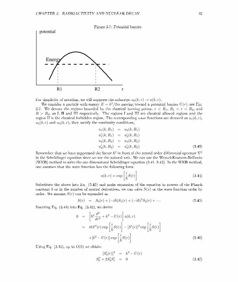
Figure 3.7: Potential barrier.
Energy
potential
R1 R2 r
For simplicity of notation, we will suppress the subscript u0(k, r)→ u(k, r).We consider a particle with energy E = k2/2m moving toward a potential barrier U(r), see Fig.
3.7. We denote the regions bounded by the classical turning points, r < R1, R1 < r < R2, andR > R2, as I, II and III respectively. The regions I and III are classical allowed regions and theregion II is the classical forbidden region. The corresponding wave functions are denoted as u1(k, r),u2(k, r) and u3(k, r), they satisfy the continuity conditions,
u1(k,R1) = u2(k,R1)
u′1(k,R1) = u′2(k,R1)
u2(k,R2) = u3(k,R2)
u′2(k,R2) = u′3(k,R2) (3.43)
Remember that we have suppressed the factor ~2 in front of the second order dierential operator ∇2
in the Schrödinger equation since we use the natural unit. We can use the Wenzel-Kramers-Brillouin(WKB) method to solve the one dimensional Schrödinger equation (3.41, 3.42). In the WKB method,one assumes that the wave function has the following form,
u(k, r) = exp
[i
~S(r)
](3.44)
Substitute the above into Eq. (3.42) and make expansion of the equation in powers of the Planckconstant ~ or in the number of spatial derivatives, we can solve S(x) or the wave function order byorder. We assume S(r) can be expanded as
S(r) = S0(r) + (−i~)S1(r) + (−i~)2S2(r) + · · · (3.45)
Inserting Eq. (3.44) into Eq. (3.42), we derive
0 =
[~2 d
2
dr2+ k2 − U(r)
]u(k, r)
= i~S′′(r) exp
[i
~S(r)
]− [S′(r)]2 exp
[i
~S(r)
]+[k2 − U(r)] exp
[i
~S(r)
](3.46)
Using Eq. (3.45), up to O(~) we obtain
[S′0(r)]2 = k2 − U(r)
S′′0 + 2S′0S′1 = 0 (3.47)

CHAPTER 3. RADIOACTIVITY AND NUCLEAR DECAY 43
Then we can solve
S0 = ±∫dr√k2 − U(r)
S′1 = −1
2[lnS′0(r)]′
→S1 = ln[k2 − U(r)]−1/4 (3.48)
Let's dene a new variable k ≡√k2 − U(r). So the wave function has the form (we resume the use
of natural unit),
u(k, r) = exp [iS(r)] =1√k
exp
(±i∫ r
r0
drk
)(3.49)
For the classically allowed region, i.e. k2 > U(r) or k is real, the general form of the wave function is
u(k, r) =C1√k
exp
(i
∫ r
r0
drk
)+
C2√k
exp
(−i∫ r
r0
drk
)=
C ′1√k
sin
(∫ r
r0
drk + C ′2
)(3.50)
where C1,2 and C ′1,2 are constants to be determined by the boundary and normalization condition.
For the classically forbidden region, i.e. k2 < U(r), k in Eq. (3.49) is purely imaginary, so the wavefunction has the following form,
u(k, r) =C1√|k|
exp
(−∫ r
r0
dr|k|)
+C2√|k|
exp
(∫ r
r0
dr|k|)
(3.51)
where C1,2 are constants to be determined by the boundary and normalization condition. One canobserve that the solution in the classically allowed region is oscillating while that in the forbiddenregion is exponential. Note that at classical turning points, the points at which k2 = U(r), the WKBsolutions in Eqs. (3.50,3.51) are not valid since they are divergent.
Now we consider the boundary at r = R1 with the classically allowed region in the left-side andthe classically forbidden region in the right-side. The wave functions in the both sides have followingcorrespondence,
2√k
sin
(∫ R1
r
drk +π
4
)⇐⇒ 1√
|k|exp
(−∫ r
R1
dr|k|)
r < R1 r > R1 (3.52)
Note that the wave function in the left-side is the superposition of an incident and reection wavewith equal amplitude (we assume the loss from transmission is small),
sin
(∫ R1
r
drk +π
4
)= −i exp
[i
(∫ R1
r
drk +π
4
)]
+i exp
[−i(∫ R1
r
drk +π
4
)](3.53)
We can rewrite the right-side wave function in Eq. (3.52) as
1√|k|
exp
(−∫ R2
R1
dr|k|)
exp
(∫ R2
r
dr|k|)
(3.54)
CHAPTER 3. RADIOACTIVITY AND NUCLEAR DECAY 44
The second factor has following correspondence to the wave function in the right side of the turningpoint at r = R2,
exp
(∫ R2
r
dr|k|)⇐⇒ − exp
[i
(∫ r
R2
drk +π
4
)]r < R2 r > R2 (3.55)
With the factor in Eq. (3.54), we obtain the wave function in the region r > R2,
u(k, r > R2) = − 1√|k|
exp
[−∫ R2
R1
dr|k|]
exp
[i
(∫ r
R2
drk +π
4
)](3.56)
So the transmission current is
j ∼ k|u(k, r > R2)|2 = exp
(−2
∫ R2
R1
dr|k|)
(3.57)
The transmission probability is then
P = exp
(−2
∫ R2
R1
dr|k|)
(3.58)
For the α decay, there are two forces in the nuclei, nuclear and Coulomb. We can assume thenuclear and Coulomb forces reach balance for the α particles which can be treated as free inside thenuclei. The potential for the α particles is
V (r) =
−V0, r < RZ1Z2e
2
r , r > R(3.59)
where Z1 = 2 and Z2 = Z. See Fig. 3.6. Let us estimate the height of potential barrier,
EB =Z1Z2e
2
R≈ 2Z × 1.44
1.2(A1/3 +A1/3α )
= 2.4Z
A1/3 +A1/3α
≈ 27 MeV for 21284 Po, (3.60)
where R ≈ 1.2(A1/3 +A1/3α ) = 9 fm.
One sees EB E0. According to classical theory the α decay cannot escape. But in quantumtheory the penetration probability is given
P = e−G = exp
(−2√
2mα
∫ b
R
√V − E0dr
)(3.61)
where b = Z1Z2e2
E0. When b/R 1,
G = 2√
2mα
∫ b
R
√Z1Z2e2
r− E0dr = 4
√2
√mα
E0Z1Z2e
2
∫ 1
ymin
√1− y2dy
≈ 4√
2
√mα
E0Z1Z2e
2
[∫ 1
0
√1− y2dy −
∫ ymin
0
√1− y2dy
]≈ 4
√2
√mα
E0Z1Z2e
2
(π
4−√R
b
)= 2√
2πZe2
√mα
E0− 8√e2mα
√ZR
= 2√
2π1
137
√3750
Z√E0
− 8√
3750/197/137√ZR
= 3.97Z√E0
− 2.98√ZR (3.62)

CHAPTER 3. RADIOACTIVITY AND NUCLEAR DECAY 45
where y ≡√
rb and ymin =
√RE0
Z1Z2e2=√
Rb . We have used the ne structure constant e2 = 1/137.
Obtaining the last line, we have used Z1 = 2, Z2 = Z, mα = 3750 MeV. In the last equality, R is inunit fm and E0 is in MeV. The collision times per second for an α particle inside the nucleus is
n =v
2R≈√
2Ekmα
1
2R≈ 3× 10²¹A−1/3E
1/2k sec−1 (3.63)
where Ek = E0 + V0 is the kinetic energy of the α particle inside the nucleus in unit MeV. Intransforming the speed v from the natural unit to cgs one, we note that it has to times the speed oflight c. Then the average life for α decay is
τ =1
λ=
1
nP≈ 3.5× 10⁻²²A1/3E
−1/2k eG (3.64)
We can take logarithm of above and obtain,
ln τ = a1 + a21√E0
, (3.65)
where a1 = ln(3.5× 10⁻²²A1/3E−1/2k )− 2.98
√ZR and a2 = 3.97Z. Eq. (3.65) was rst obtained as
an empirical law by Geiger and Nutall in 1911 and later conrmed by quantum mechanics.Let us estimate the half life of 210Po from α decay,
T1/2( 210Po) =ln 2
λ= ln 2× 3.5× 10−22A1/3E
−1/2k eG
≈ ln 2× 3.5× 10−22 × 2101/3 × (5.4)−1/2 × exp(3.97× 84/√
5.4− 2.98×√
84× 9)
≈ 6.2× 10⁻²² × exp(61.6)
≈ 4.06 days (3.66)
T1/2( 212Po) ≈ ln 2× 3.5× 10−22 × 2121/3 × (9.03)−1/2
× exp(3.97× 84/√
9.03− 2.98×√
84× 9)
≈ 4.81× 10⁻²² × exp(29)
≈ 1.98× 10⁻⁹ s (3.67)
We can compare with the data, T1/2( 210Po) = 138.4 days and T1/2( 212Po) = 3× 10⁻⁷ s.In the above simple model, we have made several approximations. (1) We have neglected the
inuence of initial and nal state wave functions. (2) we did not consider the angular momentumof alpha particles. When the angular momentum is taken into account, there will be centrifugal
potential Vcent = L(L+1)2mr2 which will modify the half life of alpha decay. (3) We used the nuclear
radius formula R = 1.2A1/3 fm, which is not correct for many heavy nuclei with strong deformation.Since the half-lives are very sensitive to the nuclear radius, it becomes a method to measure the shapeof the nuclei through α decay half-lives.
The alpha decay is strong interaction which conserves parity. The parity of an alpha particle is(−1)L where L is the quantum number of the orbital angular momentum. So parity conservationrequires the selection rule Pi = (−1)LPf , where Pi and Pf are the parity of the initial and nal staterespectively.
A full description of alpha decay using time dependent quantum mechanics can be found in Ref.[34, 35].
Exercise 11. Use the data at the IAEA nuclear data services [28] to draw the binding energyper nucleon as a function of the number of nucleons in Fig. 2.9. Also draw the α particledecay energy E0 in Eq. (3.25) as a function of the number of nucleons.
CHAPTER 3. RADIOACTIVITY AND NUCLEAR DECAY 46
Exercise 12. Calculate the half life of 23892 U from emission of 4.2 MeV α-particles. One
assumes Ek ≈ E0.
Exercise 13. In the above we do not consider the angular momentum of alpha particles.
When the angular momentum is taken into account, the centrifugal potential Vcent = L(L+1)2mr2
will modify the half life of alpha decay. Estimate its correction to T1/2( 210Po).
Exercise 14. A full description of alpha decay using time dependent quantum mechanicscan be found in Ref. [34, 35]. Read one of the articles and write a report of 2000 chinesewords.
Exercise 15. Calculate the α decay half-lives of thorium isotopes(A=220,222,224,226,228,230,232) and compare to the experimental data.
Exercise 16. Consider the alpha decay A+4Z+2X → A
ZY +α. The potential for the α particlesis
V (r) =
−V0, r < RZ1Z2e
2
r , r > R
where Z1 = 2, Z2 = Z and R ≈ 1.2(A1/3 + A1/3α ). The kinetic energy of the alpha particle
is E0, from which we can determine classical turning point b = Z1Z2e2
E0. The transmission
probability for the alpha particle to go through the Coulomb barrier is
P = e−G = exp
(−2√
2mα
∫ b
R
√V − E0dr
)
We assume b/R 1. (1) Work out the integral to express P as a function of E0, Z andR. (2) Write down the formula for the half-life of the alpha decay in terms of Ek = E0 +V0
and R.
3.4 β decay: weak interaction at work
In the α decay, when the recoil energy of the daughter nucleus is negligible, the energy of the αparticle reects its energy inside the mother nucleus. The energy spectrum is not continuous sincethe α particle and the daughter nucleus form a quasi-bound state inside the mother nucleus and thebound state energies form energy levels. Unlike the α decay, the energy spectrum of the β particle orelectron in the β decay is continuous ranging from the zero to the decay energy which is the energydierence between the initial and nal state. This poses a puzzle or a challenge for theorists. Inorder to explain the continuous energy spectra in the β decay or the 'missing' energy Pauli proposedthe neutrino hypothesis, accompanying the emission of electrons is emitted a tiny particles calledneutrinos which escape the catch of the detector. Neutrinos are spin-one-half neutral particles withvery small mass. The β decay is then written as
AZX → A
Z+1Y + e− + νe (3.68)
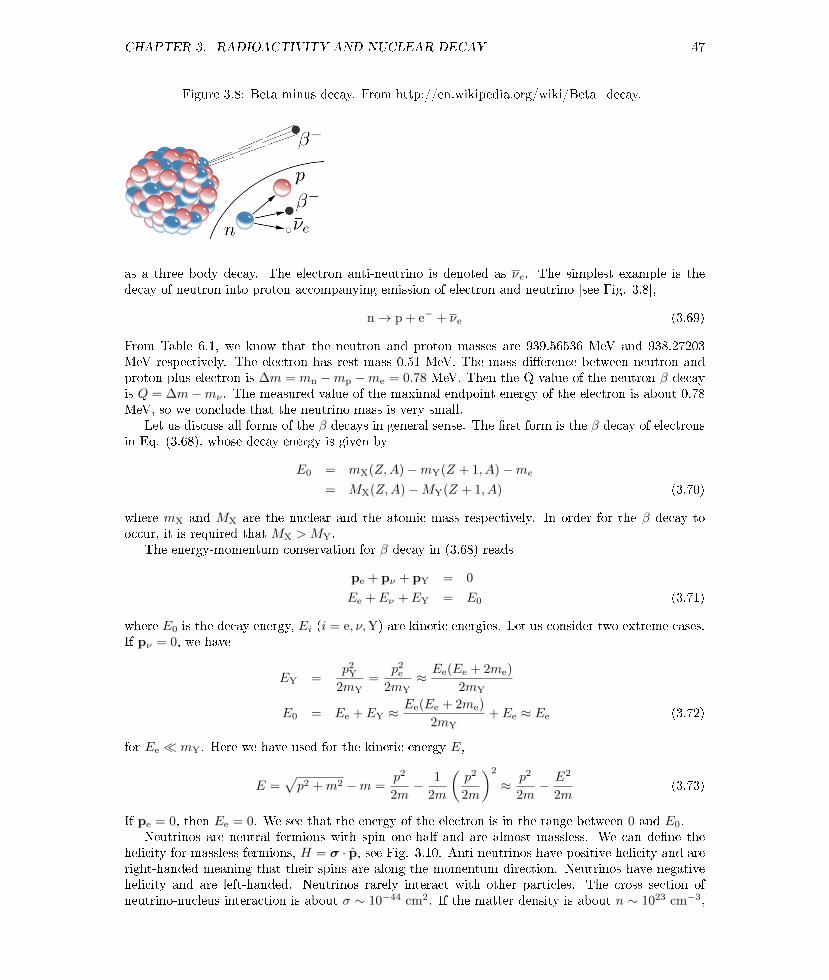
CHAPTER 3. RADIOACTIVITY AND NUCLEAR DECAY 47
Figure 3.8: Beta minus decay. From http://en.wikipedia.org/wiki/Beta_decay.
as a three body decay. The electron anti-neutrino is denoted as νe. The simplest example is thedecay of neutron into proton accompanying emission of electron and neutrino [see Fig. 3.8],
n→ p + e− + νe (3.69)
From Table 6.1, we know that the neutron and proton masses are 939.56536 MeV and 938.27203MeV respectively. The electron has rest mass 0.51 MeV. The mass dierence between neutron andproton plus electron is ∆m = mn −mp −me = 0.78 MeV. Then the Q-value of the neutron β-decayis Q = ∆m−mν . The measured value of the maximal endpoint energy of the electron is about 0.78MeV, so we conclude that the neutrino mass is very small.
Let us discuss all forms of the β decays in general sense. The rst form is the β decay of electronsin Eq. (3.68), whose decay energy is given by
E0 = mX(Z,A)−mY(Z + 1, A)−me
= MX(Z,A)−MY(Z + 1, A) (3.70)
where mX and MX are the nuclear and the atomic mass respectively. In order for the β decay tooccur, it is required that MX > MY.
The energy-momentum conservation for β decay in (3.68) reads
pe + pν + pY = 0
Ee + Eν + EY = E0 (3.71)
where E0 is the decay energy, Ei (i = e, ν,Y) are kinetic energies. Let us consider two extreme cases.If pν = 0, we have
EY =p2
Y
2mY=
p2e
2mY≈ Ee(Ee + 2me)
2mY
E0 = Ee + EY ≈Ee(Ee + 2me)
2mY+ Ee ≈ Ee (3.72)
for Ee mY. Here we have used for the kinetic energy E,
E =√p2 +m2 −m =
p2
2m− 1
2m
(p2
2m
)2
≈ p2
2m− E2
2m(3.73)
If pe = 0, then Ee = 0. We see that the energy of the electron is in the range between 0 and E0.Neutrinos are neutral fermions with spin one-half and are almost massless. We can dene the
helicity for massless fermions, H = σ · p, see Fig. 3.10. Anti-neutrinos have positive helicity and areright-handed meaning that their spins are along the momentum direction. Neutrinos have negativehelicity and are left-handed. Neutrinos rarely interact with other particles. The cross section ofneutrino-nucleus interaction is about σ ∼ 10−44 cm2. If the matter density is about n ∼ 1023 cm−3,

CHAPTER 3. RADIOACTIVITY AND NUCLEAR DECAY 48
Figure 3.9: Decay scheme for beta decay for Cobalt-60 and Gold-198. Fromhttp://en.wikipedia.org/wiki/Decay_scheme.
Figure 3.10: Neutrino helicity.
momentum−direction
spin−direction
momentum−direction
spin−direction
helicity=+1 helicity=−1

CHAPTER 3. RADIOACTIVITY AND NUCLEAR DECAY 49
Figure 3.11: The K-electron capture isotope 74Be, taken from Ref. [24].
the mean free path is about lmfp = 1/(nσ) ∼ 1016 km. Direct experimental tests of neutrinos are hardto carry out. But there are some indirect evidences for their existence, for example, the beta particlecan be emitted at any angles with respect to recoiling nucleus. The measurement of the recoil energyspectrum of an electron capture isotope is a good test of the single neutrino hypothesis. The kineticenergy of the recoiling nucleus is
EY =p2
Y
2mY=
p2ν
2mY≈ E2
0
2mY∼ MeV2
10, 000 MeV∼ 100 eV (3.74)
We see that the recoil energy is very small. In order to enlarge the recoiling energy the light nucleiare favorable. Davis Jr. measured the recoil energy of the process [24]
74Be + eK → 7
3Li + ν + 0.87 MeV (3.75)
which gave the expected result ER ∼ 56 eV.The direct detection of neutrinos was made by F. Reines and C. L. Cowan in 1959 [25]. They
measured the cross section of the following process
ν + p → n + e+ (3.76)
The anti-neutrinos were emitted from a powerful ssion reactor. They used 1400 liter liquid scintilla-tion detector as the proton source, where a cadmium compound was added to the scintillator solutionmainly of triethylbenzene for the detection of the reaction by the delayed coincidence technique.The positrons will annihilate with electrons emitting photons, while the neutrons are captured bycadmium also producing photons.
The β decay of 31H put a more stringent limit on the neutrino mass,
31H→ 3
2He + e− + νe (3.77)
The atomic masses of 31H and 3
2He are 2809.431984 MeV and 2809.413284 MeV respectively. Theatomic mass dierence between 3
1H and 32He is ∆m = MH−MHe ≈ 0.0186. The nuclear mass dierence
between 31H and 3
2He + e− becomes ∆m = (MH −me) − (MHe − 2me) −me = MH −MHe ≈ 0.0186

CHAPTER 3. RADIOACTIVITY AND NUCLEAR DECAY 50
Figure 3.12: The anti-neutrino detector used by Reines and Cowan, taken from Ref. [25].

CHAPTER 3. RADIOACTIVITY AND NUCLEAR DECAY 51
MeV. The upper limit for neutrino mass is only about 18.6 KeV. The further study of momentumspectrum of electrons gives an upper limit of only about 60 eV.
We provide two another examples for beta decays, Co-60 and Au-198, in Fig. 3.9. Co-60 is widelyused as radioactive source for radiotherapy. Co-60 mainly decay to two excited states of Ni-60 throughbeta emission with a half life of 5.27 years. The excited states of Ni-60 emit two gamma rays withenergies at 1.1732 MeV and 1.33 MeV. The decay energies are 0.31 MeV and 1.48 MeV respectively.For Au-198, it has three beta decay channels, to excited states of Hg-198 at 1.09 MeV and 0.41 MeV,and to the ground state. The excited states decay to the ground state by emitting three gamma raysof 0.68 MeV, 0.41 MeV and 1.09 MeV. The decay energies are 0.28 MeV, 0.96 MeV and 1.37 MeVrespectively.
The second form of beta decay is the β+ decay for positron emission,
AZX → A
Z−1Y + e+ + νe (3.78)
The decay energy is given
E0 = mX(Z,A)−mY(Z − 1, A)−me
= MX(Z,A)−MY(Z − 1, A)− 2me (3.79)
In order for the β+ decay to take place, one requires MX(Z,A) > MY(Z − 1, A) + 2me.The third form of beta decay is the orbital electron capture (EC),
AZX + e−i → A
Z−1Y + νe (3.80)
where e−i is the electron in the i-shell. The decay energy is
E0i = mX +me −mY −Wi
= MX(Z,A)−MY(Z − 1, A)−Wi (3.81)
where Wi is the binding energy of the electron in the atom. The K-level electron capture takes placewith the largest probability, next to it is the L-level one. When
WK > MX(Z,A)−MY(Z − 1, A) > WL (3.82)
the K-level electron capture cannot happen but the L-level one can. Since 2me Wi, the nucleiwhich can β+ decay can also capture orbital electrons.
As an example, we look at the β+ decay and EC of Zn-65:
6530Zn → 65
29Cu + e+ + νe
6530Zn + e−i → 65
29Cu + νe (3.83)
The scheme plot is shown in Fig. 3.13. There are two EC channels, whose decay energies are 0.236MeV (45%) and 1.34 MeV (53.5%). The decay energy of the β+ decay is 0.325 MeV. 64
29Cu is thenucleus where all β−, β+ and EC can happen.
There are two kinds of double β decays, one with two neutrinos produced (ββ2ν) and anotherwithout neutrinos ββ0ν.
AZX → A
Z+2Y + 2e− + 2ν, (ββ2ν)AZX → A
Z+2Y + 2e−, (ββ0ν) (3.84)
The neutrinos in 2νββ are Dirac neutrinos for which anti-neutrinos and neutrinos are dierentfermions, those in 0νββ are Majorana ones for which anti-neutrinos and neutrinos are identical.The neutrinoless double β deay (ββ0ν) is the combination of two processes,
n → p + e− + ν
ν + n → p + e− (3.85)

CHAPTER 3. RADIOACTIVITY AND NUCLEAR DECAY 52
Figure 3.13: β+ decay and electron capture of Zn-65.
No experiments so far have succeeded in proving that neutrinos are of Dirac or Majorana types. In βdecay, the nal nucleus must have a larger binding energy than the initial nucleus. For some nucleithe β decay cannot happen since the nucleus with one more proton and one less neutron has smallerbinding energy, the nucleus with two more protons and two less neutrons has larger binding energyso that the double β decay can happen. Germanium-76 is an example, which can in principle decayto selenium-76 via the double β decay. Here are isotopes which have been observed to have double βdecay: 48
20Ca,7632Ge,
8234Se,
9640Zr,
10042 Mo, 116
48 Cd, 12852 Te, 130
52 Te, 15060 Nd, 238
92 U.
Exercise 17. Write down the reaction formula for the β and β+ decay for the nucleus AZX,
where the daughter nucleus is A′
Z′Y with A′ and Z ′ the nucleon and proton numbers. Whatare conditions for these decays to take place? Express the conditions using the atomic massesof X and Y .
Exercise 18. Write down the reaction formula for the ββ2ν and ββ0ν decay for the nucleusAZX, where the daughter nucleus is A′
Z′Y with A′ and Z ′ the nucleon and proton numbers.What is the dierence in the electron energy spectra between the ββ2ν and ββ0ν decays?
Exercise 19. For following beta-type decays,
AZX → A
Z+1Y + e− + νe, (β)AZX → A
Z−1Y + e+ + νe, (β+)AZX + e−i → A
Z−1Y + νe, (EC)AZX → A
Z+2Y + 2e− + 2νe, (ββ2ν)
Using atomic masses of X and Y to express the energy, what are the energy conditions forthe reactions to take place?

CHAPTER 3. RADIOACTIVITY AND NUCLEAR DECAY 53
Figure 3.14: Double beta decay. From: http://en.wikipedia.org/wiki/Double_beta_decay.
Figure 3.15: Similarity between an electron scattering and a beta decay-type reaction. The propagatorof the W± and Z0 can be approximated as a point contact interaction due to their heavy masses.
e−
e−
e−
e−
γ
n
e−
νe
p
W±, Z0
n n
p e−
νe
Exercise 20. List all mass data for mother and daughter nuclei for nuclides which canundergo double beta decays. These are 48
20Ca,7632Ge,
8234Se,
9640Zr,
10042 Mo, 116
48 Cd, 12852 Te, 130
52 Te,15060 Nd, 238
92 U. Calculate the Q-values of each decay.
3.4.1 Fermi theory of β decay
In 1934 Fermi proposed a theory to describe the β decay. Fermi made an analogy of the β decay tothe quantum transition of two atomic states radiating light or electron-electron scatterings, see Fig.3.15. Similarly in β decay a quantum transition takes place where a neutron changes to a protonwith emission of an anti-neutrino and an electron. In quantum electrodynamics, the amplitude ofelectron-electron scatterings can be written as ψγµψψγ
µψ where ψ is a spinor eld for electrons andcan be understood as the electron wave function. Fermi then proposed the four-fermion model forthe β decay. In this subsection, we will illustrate how the model works.
Before we discuss about the Fermi theory of the β decay. Let's rst derive the Fermi golden rulefor the rate of a quantum transition process from the Schrödinger equation. Suppose the transitionis the concequence of the perturbative part of the Hamilton, Hint. The free part of the Hamilton isdenoted as H0. The Schrödinger equation reads,
i~∂ψ
∂t= (H0 +Hint)ψ (3.86)

CHAPTER 3. RADIOACTIVITY AND NUCLEAR DECAY 54
where Hint H0. The eigenstates of H0 form a complete and orthorgonal set |n〉 , n = 0, 1, 2, · · · with H0 |n〉 = En |n〉. Suppose at the initial time t = 0, the system is in one eigenstate of H0,ψ(0) = |i〉. At a later time t, the wave function is in the form,
ψ(t) =∑n
Cni(t) exp
(− i~Ent
)|n〉 (3.87)
So we have Cni(0) = δni. We can calculate the amplitude Cnk(t) by substituting the above wavefunction into the Schrödinger equation,
i~∑n1
d
dtCn1i(t) exp
(− i~En1
t
)|n1〉 =
∑n1
Cn1i(t) exp
(− i~En1
t
)Hint |n1〉 (3.88)
We can determine Cni(t) by projecting the above state on |n〉,
Cni(t) =1
i~∑n1
Cn1i(t) exp
[i
~(En − En1
)t
]〈n|Hint |n1〉
≈ 1
i~exp
[i
~(En − Ei)t
]〈n|Hint |i〉 (3.89)
where we have used Cni(t) ≈ Cni(0) = δni. Then we can solve Cni(t) as
Cni(t) = δni +1
i~
∫ t
0
dt exp
[i
~(En − Ei)t
]〈n|Hint |i〉 (3.90)
If n 6= i, we get the transition probability for |i〉 → |n〉,
Pni =1
~2
∣∣∣∣∫ t
0
dt exp
[i
~(En − Ei)t
]〈n|Hint |i〉
∣∣∣∣2 (3.91)
If Hint is independent of time, the probability for t→∞ becomes,
Pni =1
~2|〈n|Hint |i〉|2
∣∣∣∣∫ t
0
dt exp
[i
~(En − Ei)t
]∣∣∣∣2=
1
~2|〈n|Hint |i〉|2
sin2[(En − Ei)t/(2~)]
(En − Ei)2/(4~2)
→ |〈n|Hint |i〉|2 2πtδ(En − Ei), (t→∞, in natural unit) (3.92)
where we have used
limx→∞
sin2(x)
x2= πδ(x) (3.93)
Taking the density of nal states into account, we obtain the transition rate
λ =
∫dn(En) |〈n|Hint |i〉|2 2πδ(En − Ei)
= 2πρ(Ei) |〈n|Hint |i〉|2 (3.94)
where dndE = ρ(E) is the energy density of states. Eq. (3.94) is called the Fermi golden rule.
Now we deal with the β decay with the Fermi golden rule. The initial state is the state of themother nucleus and the nal state is made up of daughter nucleus, an electron and an anti-neutrino,
|i〉 =∣∣AZX⟩
= ui(x)
|f〉 =∣∣AZ+1Y, e
−, νe
⟩= uf(x)φe(xe)φν(xν) (3.95)

CHAPTER 3. RADIOACTIVITY AND NUCLEAR DECAY 55
Here ui,f are eigenstates of mother and daughter nuclei respectively, and φe and φν are the wavefunction of the electron and neutrino. Accoding to the Fermi golden rule the dierential decay ratereads
dλ = 2π |〈f|Hint |i〉|2 δ(Ef + Ee + Eν − Ei)dρ(e−, νe) (3.96)
where dρ(e−, νe) is the number of nal states for electrons and (anti-)neutrinos. The matrix elementof the Hamiltonian between the initial and nal state is
Mfi = 〈f|Hint |i〉
=
∫d3xd3xed
3xνu∗f (x)φ∗e(xe)φ∗ν(xν)Hintui(x)
= G
∫d3xd3xed
3xνu∗f (x)φ∗e(xe)φ∗ν(xν)ui(x)δ(xe − x)δ(xν − x)
= G
∫d3xu∗f (x)φ∗e(x)φ∗ν(x)ui(x) (3.97)
where we assumed the interaction part of the Hamiltonian is in a point contact form,
Hint = Gδ(xe − x)δ(xν − x) (3.98)
with G the eective coupling constant for β decay.The dierential decay rate for emitting an electron within the momentum range [ke, ke + dke] is,
dλ ≈ G2
∣∣∣∣∫ d3xu∗f (x)φ∗e(x)φ∗ν(x)ui(x)
∣∣∣∣2 2πδ(Ef + Ee + Eν − Ei)dρ. (3.99)
Assuming that the electron and the neutrino are free particles, their wave functions can be approxi-mated by the plane waves
φe =1√Veike·x
φν =1√Veikν ·x (3.100)
Substituting the above into Eq. (3.99), we obtain
dλ = G2 1
V 2
∣∣∣∣∫ d3xu∗f (x)ui(x)e−i(ke+kν)·x∣∣∣∣2 2πδ(Ef + Ee + Eν − Ei)dρ
= G2 1
V 2
V d3ke
(2π)3
V d3kν(2π)3
2πδ(Ef + Ee + Eν − Ei)|Mfi|2, (3.101)
where we have used
dρ =V d3ke
(2π)3
V d3kν(2π)3
= k2ek
2νdkedkν
V dΩe
(2π)3
V dΩν(2π)3
,
|Mfi|2 ≡∣∣∣∣∫ d3xu∗f (x)ui(x)e−i(ke+kν)·x
∣∣∣∣2 , (3.102)
where we used ke,ν ≡ |ke,ν |. Note that |Mfi|2 is dimensionless. If we neglect the neutrino massmν ≈ 0and integrate over nal state phase space where electron momenta are in the range [ke, ke + dke], Eq.(3.101) becomes
dλ = 2πG2k2edke
∫dΩe
(2π)3
∫d3kν(2π)3
δ(Ef + Ee + Eν − Ei)|Mfi|2
=G2
2π3dkek
2e (Ei − Ef − Ee)2|Mfi|2 (3.103)
CHAPTER 3. RADIOACTIVITY AND NUCLEAR DECAY 56
So the probability distribution is
dλ
dke=
G2
2π3k2
e (∆E − Ee)2|Mfi|2 (3.104)
where ∆E = Ei − Ef is the energy between the mother and daughter nucleus in the beta decay orthe decay energy.
Here we have neglected the inuence of the Coulomb eld on electrons from the nucleus. Normallythe plane wave function of an electron can be distorted in the Coulomb eld from protons inside thenucleus. The distortion to the electron wave function can be described by a Coulomb modicationfactor F (Z,Ee),
F (Z,Ee) =x
1− e−x (3.105)
where x = ±2πZe2/ve for the β∓ decay with ve = m−1e
√E2
e −m2e being the electron velocity. The
nal form of the probability distribution is now
dλ
dke=
G2
2π3k2
e (E0 − Ee)2F (Z,Ee)|Mfi|2 (3.106)
We can re-write the above spectrum as√dλ/dke
k2eF (Z,Ee)
∼ C(∆E − Ee)
= C(E0 − Te) (3.107)
where Ee = Te +me, E0 is the Q-value, and C is a constant. We can see that√
(dλ/dke)/[k2eF (Z,Ee)]
is in linear relation to Ee, which is known as the Kurie plot. From the Kurie plot we can determinethe maximum energy ∆E or the Q-value from the intercept with the energy-axis. In Eq. (3.106),we see that the electron spectrum is in the range ke = [0,
√(∆E)2 −m2
e ] ≈ [0,∆E − m2e/(2∆E)],
see Fig.3.16 for the electron momentum and kinetic energy spectra of electrons and positrons in β±
decays of 6429Cu.
If we recover the neutrino mass in Eq. (3.106) we obtain
dλ
dke=
G2
2π3k2
e (∆E − Ee)2F (Z,Ee)
√1− m2
ν
(∆E − Ee)2|Mfi|2, (3.108)
where we have used k2νdkν = kνEνdEν . The zero points read E
(0)e = ∆E and E
(0)e = ∆E±mν , where
the lowest zero point E(0)e = ∆E −mν is physical. So we can determine the neutrino mass from the
intercept with energy axis once we know ∆E.We can obtain the integrated rate from Eq. (3.106) by using dimensionless variable w ≡ Ee/me
and w0 = ∆E/me,
λ =G2
2π3
∫ E0
me
dEeF (Z,Ee)Eeke(∆E − Ee)2|Mfi|2
≈ G2m5e
2π3f(Z,w0)|Mfi|2, (3.109)
where f(Z,w0) is dened as
f(Z,w0) =
∫ w0
1
dwF (Z,w)√w2 − 1(w0 − w)2w (3.110)

CHAPTER 3. RADIOACTIVITY AND NUCLEAR DECAY 57
Figure 3.16: Momentum and kinetic energy spectra of electrons and positrons in β± decays of 6429Cu.
Taken from Fig. 5.9 on p129 of Ref. [37].
Figure 3.17: Illustration of the Fermi-Kurie plot for 3H→3 He + e− + νe. Suppose mν =30 eV, thereis dierence between massive and massless neutrinos. Taken from Fig. 5.11 on p130 of Ref. [37].

CHAPTER 3. RADIOACTIVITY AND NUCLEAR DECAY 58
Figure 3.18: T1/2f(Z,w0) for superallowed transition. Taken from Table. 5.3 on p133 of Ref. [37].
If w0 is very large, we have f(Z,w0) ∼ w50/5. The the half life is given by
T1/2 =ln 2
λ=
2π3 ln 2
G2m5ef(Z,w0)|Mfi|2
(3.111)
If we know T1/2 and |Mfi|2, we can determine the coupling G. It turns out that the quantityT1/2f(Z,w0) is almost a constant for certain type of beta decays. It is called the comparativehalf-life. For 0+ → 0+ transition, we have |Mfi|2 = 2, T1/2f(Z,w0) should be a constant, see Fig.3.18 for the experimental data. From the data G can be determined to be 0.89× 10⁻⁴ MeV · fm3 =1.16× 10⁻⁵ GeV−2. Eq. (3.111) can be put into a simple form,
T1/2f(Z,w0) ≈ 6185
|Mfi|2second
So the dimensionless coupling constant is Gm2p ≈ 1.026 × 10⁻⁵ with nucleon mass mp. This can be
compared to the counlings in strong and electromagnetic interactions whose coupling constants areof the order 1 (strong) and 10−2 (electromagnetic). We see that the strength of the β decay is muchweaker, this is why the so-called weak interaction is at work in the β decay.
We can estimate the free neutron half life from the beta decay by Eqs. (3.110,3.111). We canneglect F (Z,w). We can further neglect the recoil eect and approximate |Mfi|2 ∼ 1 + 3g2
A/g2V ∼ 5.8,
with ∆E ≈ 1.29 MeV, G = 0.89× 10⁻⁴ MeV · fm3 = 1.16× 10⁻⁵ GeV−2, and
f(Z,w0) =
∫ w0
1
dw√w2 − 1(w0 − w)2w ≈ 1.63, (3.112)
we obtain the neutron's half life
T1/2(n) ∼ 197× 10122π3 ln 2
1.152 × 10−10 × 0.515 × 1.63× 5.8(fm/c)
≈ 654 s.
The data give T1/2(n) ≈ 661 s. We see the perfect agreement between the data and the theoreticalvalue.

CHAPTER 3. RADIOACTIVITY AND NUCLEAR DECAY 59
Let us discuss about the transition amplitude |Mfi|2, Eq. (3.102). Note that the phase is verysmall (ke + kν) · x ∼ 0.1− 0.01 1, so we can make an expansion of the phase factor ei(ke+kν)·x interms of powers of (ke + kν) · x. We can also make an expansion of it in terms of spherical harmonicfunctions,
ei(ke+kν)·x =∑L=0
(2L+ 1)(−i)LjL(|ke + kν |x)PL(cos θ)
≈∑L=0
(2L+ 1)(−i)L(2L+ 1)!!
|ke + kν |LxLPL(cos θ) (3.113)
Therefore the amplitude can be written as
Mfi =∑L=0
(2L+ 1)(−i)L(2L+ 1)!!
∫d3xu∗f (x)ui(x)|ke + kν |LxLPL(cos θ)
=∑L=0
MLfi (3.114)
The matrix elements corresponding to two lowest partial waves are
ML=0fi =
∫d3xu∗f (x)ui(x)
ML=1fi = −i
∫d3xu∗f (x)ui(x)|ke + kν |xPL(cos θ) (3.115)
If ML=0fi 6= 0, it is called the allowed transition. If ML=1
fi 6= 0, it is called the rst order prohibitedtransition and etc.. The partial wave contributionML
fi drops very fast as L increases. The suppressionof higher order contributions can be seen by
ML+1fi
MLfi
∼ kr
2L+ 1∼ 10−2 (3.116)
for r ∼ 5 fm and k ∼ 1 MeV. So we see that the lowest order, L = 0, 1, contributions play the role.In the original version of the Fermi model of the beta decay, the spin part is absent. Nucleons
and leptons are spin-1/2 fermions, we can recover the spin part in Eq. (3.114),
|Mfi|2 =∑L,Seν
|ML,Seν
fi |2 (3.117)
where Seν = Se + Sν is the lepton spin. The angular momentum conservation reads
Ji = Jf + Seν + L (3.118)
where L denotes the angular momentum of the leptons, and Ji(Jf) is the nuclear spin of the mother(daughter) nucleus or the intitial (nal) nuclear state. The spin of the leptonic system Seν can be0 (singlet) or 1 (triplet), which correspond to Fermi and Gamow-Teller transition respectively. Thestrength for Fermi and Gamow-Teller transition are dierent. The coupling strength is charicaterizedby GGT/GF ∼ −1.26. For allowed transitions of the pure Fermi type (L = 0, Sl = 0), we have
|ML=0,Sl=0fi |2 = 1. For allowed transitions of the pure Gamow-Teller type, we have |ML=0,Sl=1
fi |2 = 3,
because there are three spin states. For super-allowed transition, we have |ML=0,Sl=0fi (0+ → 0+)|2 = 2
due to two pairing nucleons outside the shell in the initial 0+ state. For the mixed type decays, thereare both Fermi type and Gamow-Teller type contributions. We denote the matrix element squaredas G2
F|MF|2 +G2GT|MGT|2. From Eq. (3.114) we have parity selection rule:
PiPf = (−1)L, (3.119)

CHAPTER 3. RADIOACTIVITY AND NUCLEAR DECAY 60
Table 3.3: Classication for the beta decay. Parity selection rule: PiPf = (−1)L.
Sl = 0: Fermi Sl = 1: Gamow-TellerL = 0: allowed Ji − Jf = 0 , PiPf = 1 Ji − Jf = 0,±1, PiPf = 1
0+ → 0+: super-allowed 0+ → 1+: unique Gamow-TellerL = 1: 1st forbidden Ji − Jf = 0,±1 Ji − Jf = 0, ±1, ±2
PiPf = −1 PiPf = −1
where Pi(Pf) is the parity of the intitial (nal) nuclear state.For Seν = 0 and the allowed transition (L = 0), we get Ji − Jf = 0 and Pi = Pf , this is called
Fermi selection rule. For Seν = 1 and the allowed transition (L = 0), we get Ji − Jf = 0,±1 andPi = Pf , this is called Gamow-Teller seletion rule.
The classication for the beta decay is in Table 3.3. For various types of transitions, the decaystrengths vary to many orders of magnitude: log10[T1/2f(Z,w0)] =2.9-3.7 (super-allowed), 4.4-6.0(allowed), 6-10 (1st forbidden), above 15 (2nd forbidden), where T1/2 is in the unit of second.
Here are some examples for the allowed β-decays. (1) 148 O →14
7 N∗, 106 C →10
5 B∗, 1810Ne →18
9 F∗
and 3417Cl →34
16 S are 0+ → 0+ super-allowed Fermi-type transitions. The scheme plots for thesedecays are shown in Fig. 3.19. (2) 10
6 C →105 B (0+ → 1+), 6
2He →63 Li (0+ → 1+), 13
5 B →136
C (3/2− → 1/2−), 2812Mg →28
13 Al∗ (0+ → 1+) and 6024Cr →60
25 Mn (0+ → 1+) are Gamow-Tellertransitions. The scheme plots for these decays are shown in Fig. 3.20. There are mixed type ofdecays, here are some examples. (3) Mirror decays: n→ p(1/2+ → 1/2+), 3
1H→32 He(1/2+ → 1/2+),
137 N →13
6 C (1/2− → 1/2−), 2111Na →21
10 Ne (3/2+ → 3/2+), 4121Sc →41
20 Ca (4+ → 4+); Non-mirrordecays: 24
11Na →2412 Mg (3/2+ → 3/2+), 41
11Ar →4112 K (7/2− → 7/2−), 46
21Sc →4622 Ti (4+ → 4+),
5225Mn→52
24 Cr (2+ → 2+), 6528Ni→65
29 Cu (5/2− → 5/2−).We now discuss about the Fermi model of the orbital electron capture process. If the mass
dierence between the mother nucleus and the daughter nucleus is larger than the electron's bindingenergy, the orbital electron capture can take place. The electron capture process leads to an electronvacancy in the orbit. The lling of this vacancy by a free electron can release the binding energy byemission of X-rays or Auger electrons. The decay constant can be obtained through the Fermi goldenrule,
dλEC = 2π|Mfi|2δ(Eν − E0)dn
dEνdEν , (3.120)
where E0 is the Q-value of the process and
Mfi = G
∫d3xu∗f (x)φ∗ν(x)φe(x)ui(x),
dn
dEν= V
1
2π2E2ν . (3.121)
Here φe(x) is the electron wave function in the atomic shell. Capture is most likely for 1s electronsin the K-shell, since the s-wave function is maximal at the origin,
φe(x) =1√π
(Ze2me)3/2exp(−Ze2me|x|). (3.122)
The neutrino wave function is still a plane wave, φν = 1√Veikν ·x. Then we have
|Mfi|2 = G2 1
V
1
π(Ze2me)3|Mfi|2,
Mfi =
∫d3xu∗f (x)ui(x)exp(−ikν · x− Ze2me|x|), (3.123)

CHAPTER 3. RADIOACTIVITY AND NUCLEAR DECAY 61
Figure 3.19: The scheme plots for the allowed β-decays of the Fermi type. The half-lives are shownas log10(fT1/2). From IAEA database NuDat 2.6 at http://www.nndc.bnl.gov/nudat2/.

CHAPTER 3. RADIOACTIVITY AND NUCLEAR DECAY 62
Figure 3.20: The scheme plots for the allowed β-decays of the Gamow-Teller type. The half-lives areshown as log10(fT1/2). From IAEA database NuDat 2.6 at http://www.nndc.bnl.gov/nudat2/.

CHAPTER 3. RADIOACTIVITY AND NUCLEAR DECAY 63
where Mfi is dimensionless. So after integration Mfi is replaced by its average value, the decay rateor constant is then
λEC =G2
π2(Ze2me)3|Mfi|2E2
ν .
We have taken into account that there are two 1s electrons in the K-shell. We see that the decayconstant is proportional to Z3.
Now we calculate the cross section of the inverse beta decay processes described by
AZX + νe → A
Z+1Y + e−,AZX + νe → A
Z−1Y + e+. (3.124)
The simplest inverse beta decays are
p + νe → n + e+,
n + νe → p + e−. (3.125)
The transition rate for the inverse reaction is given by
dλinv−b = 2π|Mfi|2δ(Ee −∆E)dn
dEedEe (3.126)
where ∆E = Ei + Eν − Ef , anddn
dEe=
V
2π2keEe (3.127)
After integration, we obtain
λinv−b = 2πG2 1
V 2|Mfi|2
dn
dEe=
1
πVG2peEe|Mfi|2
=1
πVG2m2
e |Mfi|2w√w2 − 1 (3.128)
where the dimensionless nuclear matrix element Mfi is dened by
Mfi =
∫d3xu∗f (x)ui(x)ei(kν−ke)·x (3.129)
In general both Fermi-type and Gamow-Teller type reactions are present,
|Mfi|2 = |Mfi(F )|2 +G2
GT
G2F
|Mfi(GT)|2 (3.130)
Note that GF ≈ G. The cross section is then given by
σinv−b =λinv−b
Fν= λinv−bV/c
=1
πG2m2
ew√w2 − 1|Mfi|2 (3.131)
Using the value |Mfi|2 ≈ 5, we can estimate the magnitude of σinv−b for e.g. w = 3: σinv−b ∼20× 10−44 cm2.
In real situations we have to determine the electron energy from energy-momentum conservation.We assume the inverse beta decay only aect the nucleon inside the nucleus. Then we have followingequations from energy-momentum conservation in the center-of-mass frame,
pcν = pci
pce = pcf
Ecν +√p2
ci +m2p =
√p2
ce +m2e +
√p2
cf +m2n (3.132)
CHAPTER 3. RADIOACTIVITY AND NUCLEAR DECAY 64
We can express Ece as a function of pcν
Ece =(pcν +
√p2
cν +m2p)2 +m2
e −m2n
2(pcν +√p2
cν +m2p)
(3.133)
The neutrino energy in the c.m.s. is related to that in the lab frame,
pcν = γc(pν − βcEν) =1− βc√1− β2
c
pν (3.134)
where γc = 1√1−β2
c
and βc = pνpν+mp
. Then we transform to the lab frame where the initial state
nucleon is static,
Ee = γc(Eec + βcpec cos θce) (3.135)
We can take average over θce for Ee, so we get the average electron energy in the lab frame, Ee = γcEce,or explicitly,
〈Ee〉 = γc
(pcν +√p2
cν +m2p)2 +m2
e −m2n
2(pcν +√p2
cν +m2p)
(3.136)
Substituting w = 〈Ee〉 /me into Eq. (3.131), we can obtain the cross section as a function of theneutrino energy.
Exercise 21. When the neutrino has a mass, what happens to the electron energy spectradλdEe
as Ee → ∆E.
Exercise 22. Calculate the cross section of the inverse beta decay p + νe → n + e+ andn + νe → p + e− for pν = [0, 10]me. One should use exact masses for proton and neutron,i.e. take the mass dierence into acount.
Exercise 23. Read the article about solar neutrino problem in Ref. [36]. Write a reportabout it in 2000 chinese words.
Exercise 24. Find as many as possible the super-allowed and unique Gamow-Teller β decaysand in the IAEA database NuDat. For each decay, please list the decay reaction formula andthe quantity log(ft) for the half life.

CHAPTER 3. RADIOACTIVITY AND NUCLEAR DECAY 65
Figure 3.21: The parity violation in the β decay.
neutrino
electron
electron
neutrino
reflectionB
Cobalt
s=4s=5
Nickel
Exercise 25. The half-life of the beta decay is given by
T1/2 =ln 2
λ=
2π3 ln 2
G2m5ef(Z,w0)|Mfi|2
where G = 0.88×10⁻⁴ MeV · fm3 = 1.15×10⁻⁵ GeV−2, w0 = ∆E/me with the decay energy∆E and electron mass me = 0.511 MeV. For w0 1, we can approximate f(Z,w0) ∼ w5
0/5.For a pure Fermi transition (L = 0, Seν = 0), we have |Mfi|2 = 1. For a pure Gamow-Tellertransition (L = 0, Seν = 1), we have |Mfi|2 = 3, because there are three spin states. Forsuper-allowed transition (0+ → 0+), we have |Mfi|2 = 2 due to two pairing nucleons outsidethe shell in the initial 0+ state. See Fig. 3.19 for super-allowed transition of 14
8 O →147 N∗.
Calulate T1/2 for such a beta decay in the unit of second.
3.4.2 Parity violation in β decay
In 1950s there was a τ − θ puzzle that seemingly identical strange mesons θ+ and τ+ can decay intotwo and three pions respectively,
θ+ → π+ + π0
τ+ → π+ + π+ + π−
Considering a pion has negative parity and the decay occurs in s-wave, it seems that θ+ and τ+ aredierent particles with opposite parity. But actually they are all kaons and parity is violated in weakdecays.
In 1957 C.S. Wu and her collaborators measured the electron distribution in the β decay ofpolarized cobalt ,
6027Co → 60
28Ni + e− + νe (3.137)
They found that electrons are predominantly emitted opposite to the nuclear spin. Under the paritytransformation r → −r, the magnetic eld and the spin are invariant while the mometum changes

CHAPTER 3. RADIOACTIVITY AND NUCLEAR DECAY 66
the direction, i.e.
B → B
s → s
p → −p (3.138)
Along the direction of the magnetic eld, a cobalt nucleus carries a spin of 5~ while a nickel nucleuscarries a spin of 4~. The dierence in spin is compensated by the emitted electron and anti-neutrino.Since the anti-neutrino is right-handed (the spin of the anti-neutrino is along its momentum), theelectron is predominantly emitted opposite to the direction of the nuclear spin, see the left panel ofFig. 3.21.
Exercise 26. Wu and her collaborators measured the electron distribution in the β decay ofpolarized cobalt, 60
27Co → 6028Ni + e− + νe. Describe the main result of the experiment and
explain why the result indicates that the parity is violated.
3.5 γ decay: electromagnetic interaction at work
Nuclei are many body systems of nucleons which interact via nuclear force or strong interaction. Anucleus can stay in some quantum states with specic energies. By external perturbation a nucleuscan be excited to higher energetic states and can jump onto its ground state by radiating photons(for example, the nuclei normally stay in their excited states right after the α and β decay).
3.5.1 Classical electrodynamics for radiation eld
Classical electrodynamics can be summarized by Maxwell equations,
∇ ·E = 4πρ,
∇×B =4π
cj +
1
c
∂E
∂t,
∇ ·B = 0,
∇×E = −1
c
∂B
∂t. (3.139)
From the last two equations, we can dene scalar and vector potential φ(t,x) and A(t,x),
B = ∇×A
E = −∇φ− 1
c
∂A
∂t(3.140)
The above equations are invariant under gauge transformation
φ′ = φ+1
c
∂f
∂tA′ = A−∇f (3.141)
where f(t,x) is a function of space and time. Eq. (3.140) satises the last two equations of (3.139)automatically. Then inserting Eq. (3.140) into the rst two equations of (3.139), we obtain
−∇2φ− 1
c
∂
∂t∇ ·A = 4πρ
1
c2∂2A
∂2t−∇2A +∇(∇ ·A) +
1
c
∂
∂t∇φ =
4π
cj, (3.142)

CHAPTER 3. RADIOACTIVITY AND NUCLEAR DECAY 67
We choose the Coulomb gauge,∇ ·A = 0 (3.143)
and consider the free space where ρ = 0 and j = 0. Then Eq. (3.145) becomes
∇2φ = 0
1
c2∂2A
∂2t−∇2A +
1
c
∂
∂t∇φ =
4π
cj, (3.144)
We can further set φ = 0 as a solution to Poisson equation ∇2φ = 0 in free space with boundarycondition φ|x→∞ = 0. Then we obtain the wave equation for radiation
1
c2∂2A
∂2t−∇2A = 0 (3.145)
A vector eld satisfying the Coulomb gauge is called a transverse eld. We consider a solution to thewave equation (3.145)
A(t,x) = A0ei(k·x−ωt) (3.146)
with k2 = ω2/c2. The Coulomb gauge gives transverse condition
k ·A = 0 (3.147)
Such waves satisfying transverse condition are called radiation elds. Now we collect all equationswe need for describing radiation,
B = ∇×A
ET = −1
c
∂A
∂t∇ ·A = 0
1
c2∂2A
∂2t−∇2A = 0 (3.148)
where we have denoted ET as the transverse electric eld. The Hamiltonian for radiation eld is
Hrad =1
8π
∫d3x(E2
T + B2) (3.149)
In order to quantize the radiation eld, we consider a box of length L and volume V = L3. Theperiodic condition reads
A(t,x ∈ boundary) = constant (3.150)
We choose the following complete set of transverse orthonormal vectors which satisfy the aboveperiodic boundary condition,
1√Vε(r,k)eik·x (3.151)
where ε(r,k) with r = 1, 2 are two perpendicular real unit vectors and
k =2π
L(n1, n2, n3), n1, n2, n3 = 0,±1,±2, · · · (3.152)
The polarization vectors ε(r,k) satisfy following orthogonal and transverse conditions
ε(r,k) · ε(s,k) = δrs, k · ε(r,k) = 0 (3.153)
Then the vector potential can be expanded in this complete set of transverse orthonormal vectors asFourier series,
A(t,x) =∑k,s
(2π
V ωk
)1/2
ε(s,k)[a(t, s,k)eik·x + a∗(t, s,k)e−ik·x] (3.154)

CHAPTER 3. RADIOACTIVITY AND NUCLEAR DECAY 68
where ωk = k. We see that A(t,x) in the above form is real. Substituting Eq. (3.154) into Eq.(3.145), we get
∂2a(t, s,k)
∂t2+ ω2
ka(t, s,k) = 0 (3.155)
So we can determine the time dependent part as
a(t, s,k) = a(s,k)e−iωkt (3.156)
Then the vector potential in (3.154) becomes
A(t,x) =∑k,s
(2π
V ωk
)1/2
ε(s,k)[a(s,k)e−iωkt+ik·x + a∗(s,k)eiωkt−ik·x] (3.157)
The Hamiltonian (3.149) can be evaluated as
Hrad =1
8π
∫d3x
[(∂A
∂t
)2
+ (∇×A)2
]=
∑k,s
ωka(s,k)a∗(s,k) (3.158)
The rst term(∂A∂t
)2is evaluated as
∂A
∂t= −i
∑k,s
(2π
V ωk
)1/2
ε(s,k)ωk[a(s,k)e−iωkt+ik·x − a∗(s,k)eiωkt−ik·x]
(∂A
∂t
)2
= −i∑k,s
∑k1,s1
2π
V(ωkωk1)1/2ε(s,k) · ε(s1,k1)
×[a(s,k)e−iωkt+ik·x − a∗(s,k)eiωkt−ik·x]
×[a(s1,k1)e−iωk1 t+ik1·x − a∗(s1,k1)eiωk1 t−ik1·x]∫d3x
(∂A
∂t
)2
= −∑k,s
∑k1,s1
2π
V(ωkωk1)1/2ε(s,k) · ε(s1,k1)
×[a(s,k)a(s1,k1)e−iωkt−iωk1 t∫d3xei(k+k1)·x
−a(s,k)a∗(s1,k1)e−iωkt+iωk1 t∫d3xei(k−k1)·x
−a∗(s,k)a(s1,k1)eiωkt−iωk1 t∫d3xe−i(k−k1)·x
+a∗(s,k)a∗(s1,k1)eiωkt+iωk1 t∫d3xe−i(k+k1)·x]
=∑k,s
4πωka(s,k)a∗(s,k) + I1 (3.159)
where we have used∫d3xeik·x = V δk,0, and I1 denotes the oscillating terms ∼ e±2iωkt,
I1 = −∑k,s
∑s1
2πωkε(s,k) · ε(s1,−k)
×[a(s,k)a(s1,−k)e−2iωkt + a∗(s,k)a∗(s1,−k)e2iωkt (3.160)

CHAPTER 3. RADIOACTIVITY AND NUCLEAR DECAY 69
we will see it will cancel the same term in (∇×A)2. The second term (∇×A)2 is evaluated as
∇×A = i∑k,s
(2π
V ωk
)1/2
k× ε(s,k)[a(s,k)e−iωkt+ik·x − a∗(s,k)eiωkt−ik·x]
(∇×A)2 = −∑k,s
∑k1,s1
2π
V(ωkωk1)−1/2[k× ε(s,k)] · [k1 × ε(s1,k1)]
×[a(s,k)e−iωkt+ik·x − a∗(s,k)eiωkt−ik·x]
×[a(s1,k1)e−iωk1 t+ik1·x − a∗(s1,k1)eiωk1 t−ik1·x]∫d3x(∇×A)2 = −
∑k,s
∑k1,s1
2π
V(ωkωk1)−1/2[k× ε(s,k)] · [k1 × ε(s1,k1)]
×[a(s,k)a(s1,k1)e−iωkt−iωk1 t∫d3xei(k+k1)·x
−a(s,k)a∗(s1,k1)e−iωkt+iωk1 t∫d3xei(k−k1)·x
−a∗(s,k)a(s1,k1)eiωkt−iωk1 t∫d3xe−i(k−k1)·x
+a∗(s,k)a∗(s1,k1)eiωkt+iωk1 t∫d3xe−i(k+k1)·x]
=∑k,s
4πωka(s,k)a∗(s,k)− I1 (3.161)
where we have used
[k× ε(s,k)] · [k1 × ε(s1,k1)] = −k1 × [k× ε(s,k)] · ε(s1,k1)
= −[k1 · ε(s,k)][k · ε(s1,k1)]
+[k · k1][ε(s,k) · ε(s1,k1)] (3.162)
The combinging Eq. (3.159) and (3.161), we get Eq. (3.158).
Exercise 27. Derive the classical Hamiltonian in Eq. (3.158) using the momentum decom-position for the classical eld in Eq. (3.157).
3.5.2 Quantization of radiation eld
The quantization of radiation eld can be done by treating a(s,k) and a∗(s,k) as creation anddestruction operator. Then we impose following commutation relations[
a(s,k), a†(s1,k1)]
= δs,s1δk,k1
[a(s,k), a(s1,k1)] =[a†(s,k), a†(s1,k1)
]= 0 (3.163)
The vector potential is then an operator,
A(t,x) =∑k,s
(2π
V ωk
)1/2
ε(s,k)[a(s,k)e−iωkt+ik·x + a†(s,k)eiωkt−ik·x] (3.164)
The Hamiltonian as an operator is written in the form
Hrad =∑k,s
ωk[a†(s,k)a(s,k) +1
2] (3.165)

CHAPTER 3. RADIOACTIVITY AND NUCLEAR DECAY 70
The number operator for mode (s,k) is given by
N(s,k) = a†(s,k)a(s,k) (3.166)
Its eigenstate is then
|n(s,k)〉 =[a†(s,k)]n(s,k)√
n(s,k)!|0〉 (3.167)
One can check
a(s,k) |n(s,k)〉 =√n(s,k) |n(s,k)− 1〉
a†(s,k) |n(s,k)〉 =√n(s,k) + 1 |n(s,k) + 1〉
a†(s,k)a(s,k) |n(s,k)〉 = n(s,k) |n(s,k)〉
The eigenfunction of radiation Hamiltonian Hrad is then a product of such states for a set of modes,
|A〉 =∏ki,si
|n(si,ki)〉 (3.168)
The energy is then
E = 〈A|Hrad |A〉 =∑k,s
ωk[n(s,k) +1
2] (3.169)
Now we can use creation and destruction operators to express the momentum of electromagnetic eld,
P =1
4π
∫d3xET ×B
= − 1
4π
∫d3x
∂A
∂t× (∇×A)
= − 1
4π
∑k,s
∑k1,s1
2π
V
(1
ωkωk1
)1/2
ωkk1[ε(s,k) · ε(s1,k1)]
×∫d3x[a(s,k)e−iωkt+ik·x − a†(s,k)eiωkt−ik·x]
×[a(s1,k1)e−iωk1t+ik1·x − a†(s1,k1)eiωk1t−ik1·x]
=1
4π
∑k,s
∑k1,s1
2π
V
(1
ωkωk1
)1/2
ωkk1[ε(s,k) · ε(s1,k1)]
×∫d3x[a(s,k)a†(s1,k1)e−i(ωk−ωk1)t+i(k−k1)·x
+a†(s,k)a(s1,k1)ei(ωk−ωk1)t−i(k−k1)·x]
=∑k,s
k[a†(s,k)a(s,k) + 1/2] =∑k,s
k[N(s,k) +1
2] (3.170)
Exercise 28. Derive the quantized energy momentum of the radiating EM system in Eqs.(3.165,3.170) using the quantized eld in Eq. (3.164).

CHAPTER 3. RADIOACTIVITY AND NUCLEAR DECAY 71
3.5.3 Interaction of radiation with matter
Now we can add matter and matter-eld interaction part of Hamiltonian. Consider a system of pointcharged particles with mass mi and charge qi, the matter part of Hamiltonian reads,
Hm =∑i
1
2mi(pi − qiAi)
2
=∑i
1
2mip2i −
∑i
qi2mi
(pi ·Ai + Ai · pi) +∑i
q2i
2miA2i
=∑i
1
2mip2i −
∑i
qimi
Ai · pi +∑i
q2i
2miA2i
≡ H0 +HI (3.171)
where H0 is the free part and HI is the interaction part of particles and elds. Here we have used
pi ·Ai + Ai · pi = −i∇i ·Ai − iAi · ∇i = −2iAi · ∇i − i(∇i ·Ai) = −2iAi · ∇i (3.172)
under the Coulomb gauge condition. Here we have denoted Ai = A(xi) and Bi = B(xi). We canlook at the term Ai · pi, with A = 1
2B × r, we have qimi
Ai · pi = qi2mi
Bi · Li with Li = ri × pi isthe orbital angular momentum of particle i. So this term is actually the interaction energy of themagnetic moment from the orbital angular momentum in a magnetic eld. Similarly there shouldalso be a term gi
qi2mi
σ · Bi for spin angular momentum σ if the particle has spin, where gi is theg-factor of the particle's spin magnetic moment. For neutrons with qi = 0, the spin magnetic momentwould be vanishing which is not true, in order to avoid this problem, we can write the spin magneticmoment term as gi
e2mi
σ ·Bi where e is the absolute value of the electron charge, all information ofthe magnetic moment is contained in gi.
The electromagnetic energy is denoted as Hem,
Hem =1
8π
∫d3x(E2 + B2) (3.173)
where E = EL + ET is the full electric eld. The electric part of the electromagnetic is
1
8π
∫d3xE2 =
1
8π
∫d3x(EL + ET)2
=1
8π
∫d3x(E2
L + E2T)
=1
2
∫d3xd3x′
ρ(t,x)ρ(t,x′)
|x− x′| +1
8π
∫d3xE2
T (3.174)
In order to prove the above equation, we can use
EL = −∇φ, ET = −∂A
∂t(3.175)
and the Coulmob gauge condition ∇ · A = 0. The mixed electric energy term for transverse andlongitudinal electric elds cna be proved to be vanishing,∫
d3xEL ·ET =
∫d3x(∇φ) · ∂A
∂t
=
∫d3x∇ ·
(φ∂A
∂t
)−∫d3xφ∇ ·
(∂A
∂t
)= φ
∂A
∂t
∣∣∣∣boundary
−∫d3xφ
∂
∂t∇ ·A = 0 (3.176)

CHAPTER 3. RADIOACTIVITY AND NUCLEAR DECAY 72
using the Coulmob gauge condition. The longitudinal electric energy beocmes∫d3xE2
L =
∫d3x(∇φ)2 = −
∫d3xφ∇2φ = 4π
∫d3xφρ
= 4π
∫d3xd3x′
1
|x− x′|ρ(t,x)ρ(t,x′)
where we have used
φ(t,x) =
∫d3x′
ρ(t,x′)
|x− x′| (3.177)
For discrete system of charged particles, we can further derive∫d3xE2
L = 4π
∫d3xd3x′
1
|x− x′|∑i
qiδ(x− xi)∑j
qjδ(x′ − xj)
= 4π∑i 6=j
qiqj|xi − xj |
(3.178)
where we have usedρ(t,x) =
∑i
qiδ(x− xi) (3.179)
So we can dene the Coulomb part of electric energy HC which comes from the longitudinal electriceld,
HC =1
2
∑i 6=j
qiqj|xi − xj |
(3.180)
Therefore, we can summarize the total Hamiltonian as
H = Hm +Hem = H0 +HI +HC +Hrad (3.181)
where
H0 =∑i
1
2mip2i
HI = −∑i
qimi
Ai · pi +∑i
q2i
2miA2i −
∑i
gie
2miσ ·Bi
HC =1
2
∑i6=j
qiqj|xi − xj |
Hrad =1
8π
∫d3x(E2
T + B2) (3.182)
Here we have added a spin-magnetic-eld coupling term into HI.Let us calculate the transition amplitude of an atom or a nucleus between two energy states of
electrons or nuclear by absorption of emission of one photon, a→ b +γ, through the coupling Ai ·pi.The initial/nal states for atom or nucleus and photons are as follows
initial = |a〉 |n(s,k)〉final = |b〉 |n(s,k)± 1〉 (3.183)
The transition amplitude is then
Mfi = 〈b, n(s,k)± 1|HI |a, n(s,k)〉= i
∑i
qimi〈b, n(s,k)± 1|Ai · ∇i |a, n(s,k)〉 (3.184)

CHAPTER 3. RADIOACTIVITY AND NUCLEAR DECAY 73
Note that we have neglected A2 term since it is of quadratic order in the electric charge.First we consider the photon emission case. Inserting Eq. (3.164) into Eq. (3.184), we obtaine
the amplitude for photon emission,
Mfi = i∑k1,s1
(2π
V ωk1
)1/2
〈n(s,k) + 1| a†(s1,k1) |n(s,k)〉
×ε(s1,k1) · 〈b|∑i
qimi
eiωk1t−ik1·xi∇i |a〉
= i
(2π
V ωk
)1/2√n(s,k) + 1ε(s,k) · 〈b|
∑i
qimi
eiωkt−ik·xi∇i |a〉 (3.185)
Following the Fermi golden rule, we obtain the transition rate by taking an integral over the photonmometum and a sum over the photon spin state,
λa→b+γ = 2π
∫V d3k
(2π)3δ(Eb + ωk − Ea)
∑s=±|Mfi|2
=1
2π
∫dΩkdkδ(Eb + ωk − Ea)ωk
∑s=±
[n(s,k) + 1]
×∣∣∣∣∣ε(s,k) · 〈b|
∑i
qimi
e−ik·xi∇i |a〉∣∣∣∣∣2
(3.186)
After completing the integration over the photon energy to remove the energy conservation deltafunction, we arrive at
λa→b+γ =ωk2π
[n(k) + 1]∑s=±1
∫dΩk
×∣∣∣∣∣ε(s,k) · 〈b|
∑i
qimi
e−ik·xi∇i |a〉∣∣∣∣∣2
(3.187)
where we have used ωk = Ea − Eb = |k| and n(k) = (1/2)∑s=± n(s,k).
For photon absorption b + γ → a, we derive a similar formula
Mfi = i∑k1,s1
(2π
V ωk1
)1/2
〈n(s,k)− 1| a(s1,k1) |n(s,k)〉
×ε(s1,k1) · 〈a|∑i
qimi
e−iωk1t+ik1·xi∇i |b〉
= i
(2π
V ωk
)1/2√n(s,k)ε(s,k) · 〈a|
∑i
qimi
e−iωkt+ik·xi∇i |b〉 (3.188)
The transition rate reads,
λb+γ→a = 2π
∫V d3k
(2π)3δ(Eb + ωk − Ea)
∑s=±|Mfi|2
=1
2πdΩkdkδ(Eb + ωk − Ea)ωkn(k)
×∑s=±1
∣∣∣∣∣ε(s,k) · 〈a|∑i
qimi
eik·xi∇i |b〉∣∣∣∣∣2
(3.189)

CHAPTER 3. RADIOACTIVITY AND NUCLEAR DECAY 74
which has the following form after completing the integration over the photon energy
λb+γ→a =ωk2πn(k)
∑s=±1
∫dΩk
×∣∣∣∣∣ε(s,k) · 〈a|
∑i
qimi
eik·xi∇i |b〉∣∣∣∣∣2
(3.190)
Now we look at the simplest case, the electric dipole radiation at the long wave length limit. Atthis limit the wavelength of radiation is much larger than the size of the atom or the nucleus, so wecan approximate k ·x ≈ 0 or e−ik·x ≈ 1. Then the matrix element in Eq. (3.187) can be put into theform,
〈b|∑i
qimi∇i |a〉 = ωk 〈b|
∑i
qixi |a〉 ≡ ωkDba (3.191)
where we have dened the electric dipole moment Dba = 〈b|∑i qixi |a〉. Here we have used
∇ = ip = imdx
dt= m[x, H0] (3.192)
Then the photon emission/absorption rate in Eqs. (3.187,3.190) becomes
λa→b+γ =ω3k
2π[n(k) + 1]
∑s=±1
∫dΩk |ε(s,k) ·Dba|2
λb+γ→a =ω3k
2πn(k)
∑s=±1
∫dΩk |ε(s,k) ·Dab|2 (3.193)
Note that we have |Dab|2 = |D∗ba|2. If there is no other photons in the environment, we can setn(k) = 0(1) for the process a→ b + γ (b + γ → a), the above rates become
λa→b+γ = λb+γ→a =ω3k
2π
∑s=±1
∫dΩk |ε(s,k) ·Dba|2 (3.194)
The power of radiation is given by,
Iω = λa→b+γωk =ω4k
2π
∑s=±1
∫dΩk |ε(s,k) ·Dba|2 (3.195)
Suppose the photon is emitted along the z-axis (k is along the z-axis) and Dba is in the plane ofε(1,k) and k, so Dba is perpendicular to ε(2,k). Suppose the angle between Dba and k is θ, theabove integral of matrix element becomes∑
s=±1
∫dΩk |ε(s,k) ·Dba|2 =
∫dΩk |ε(1,k) ·Dba|2
=
∫dΩk |Dba|2 sin2 θ =
8π
3|Dba|2 (3.196)
So the radiation power turns out to be
Iω =4
3ω4k |Dba|2 (3.197)
which is consistent to the result of classical electrodynamics.

CHAPTER 3. RADIOACTIVITY AND NUCLEAR DECAY 75
We now look at the electric quadrupole radiation by considering the linear order term ∼ k · x inthe phase factor e−ik·x in Eq. (3.187). For simplicity of notation, we suppress the subscript i whichlabels the charged particles, and we have
q
m(k · x)(ε · p) = C+ + C− (3.198)
where C± is dened by
C± ≡ q
2m[(k · x)(ε · p)± (k · p)(ε · x)] (3.199)
We focus on C+ which corresponds to quadrupole radiation,
C+ =q
2m[(k · x)(ε · p) + (k · p)(ε · x)]
=q
2[(k · x)ε · dx
dt+ (k · dx
dt)(ε · x)]
=1
6qd
dt[3(k · x)(ε · x)− x2(ε · k)]
=1
6εikj
d
dtQij = −i1
6εikj [Qij , H0] (3.200)
where we used ε · k = 0 and we have dened Qij = q(3xixj − x2δij). We have also used the
Schroedinger equation for the operator O, i ddtO = [Q, H0]. Substituting Eq. (3.200) into Eq. (3.187)and setting n(k) = 0, we obtain the emission rate
λa→b+γ =ωk72π
∑s=±1
∫dΩk
∣∣∣∣∣εi(k, s)kj 〈b|∑n
[Q(n)ij , H0] |a〉
∣∣∣∣∣2
=ω3k
72π
∑s=±1
∫dΩk
∣∣∣∣∣εi(k, s)kj 〈b|∑n
Q(n)ij |a〉
∣∣∣∣∣2
(3.201)
where n labels all charged particles in the system. This gives the electric quadrupole transition rate.The absorption rate can be similarly derived from Eq. (3.190).
Let us look at the C− term in Eq. (3.199),
C− =q
2m[(k · x)(ε · p)− (k · p)(ε · x)] =
q
2m(k× ε) · (x× p)
= (k× ε) · µLNote that k×ε comes from B = ∇×A, so C− ∼ −µL ·B is from the interaction of magnetic momentin magnetic eld. So this term corresponds to the magnetic dipole transition. If the particle has spin,there is also a term (k× ε) · µS . So we can combine µS and µL and write the term as
C− → (k× ε) · (µL + µS) (3.202)
We then obtain the magnetic dipole transition rate from
λa→b+γ =ω3k
2π
∑s=±1
∫dΩk
∣∣∣∣∣[k× ε(k, s)] · 〈b|∑n
(µ(n)L + µ
(n)S ) |a〉
∣∣∣∣∣2
(3.203)
where n labels all charged particles in the system.From Eq. (3.193) we further obtain
λa→b+γ
λb+γ→a=
n(k) + 1
n(k)(3.204)

CHAPTER 3. RADIOACTIVITY AND NUCLEAR DECAY 76
If we assume equilibrium,
N(A)λa→b = N(B)λb→a (3.205)
then we have N(a) ∝ e−Ea/T and N(b) ∝ e−Eb/T ,
N(a)
N(b)=
n(k)
n(k) + 1= e−ωk/T
n(k) =1
eωk/T − 1(3.206)
which is Bose-Einstein distribution.
3.5.4 Multipole expansion
Let's rst look at electric and magnetic dipole radiation. A static electric dipole is made up of twoopposite charges (q,−q) separated by a distance d along the z-axis. The electric dipole moment isDE = qd. Suppose it is oscillating in time, DE = qd cos(ωt), it will induce an electric current I in thez-direction which produces a magnetic eld tangent to the circle parallel to the xy-plane and centeredalong the z-axis. So the magnetic eld is perpendicular to the coordinate vector x, i.e. x ·B(E) = 0.
The electric eld is determined by E(E) = B(E) × k with k the wave vector. An oscillating magneticmoment is expressed as DM = Ia cos(ωt) where I and a denote the electric current density and thearea of a coil. Similarly it will induce a circular electric eld perpendicular to the coordinate vectorx, i.e. x ·E(M) = 0. The magnetic eld is determined by B(M) = k×E(M). See Fig. 3.22.
Both electric and magnetic dipole radiation give the same power distribution but radiation eldshave opposite parity under the transformation x → −x. The electric dipole moment is odd underthe transformation, therefore the magnetic eld it induces changes sign, i.e. B(E)(−x) = −B(E)(x),E(E)(−x) = −E(E)(x). The magnetic dipole moment is even under the transformation x → −x, sothe elds do not change sign, i.e. B(M)(−x) = B(M)(x), E(M)(−x) = E(M)(x).
The wave equation for the vector potential in free space reads
1
c2∂2A
∂2t−∇2A = 0 (3.207)
Let us assume that the vector potential has an oscillating part of the form of e−iωt. The wave equationbecomes
(∇2 + k2)A(k,x) = 0 (3.208)
where k ≡ |k| = ω and ∇2 is given by
∇2 =1
r2
∂
∂r
(r2 ∂
∂r
)− 1
r2L2
L = −ix×∇
L2 = −[
1
sin θ
∂
∂θ
(sin θ
∂
∂θ
)+
1
sin2 θ
∂2
∂φ2
]Here L is the angular momemtum operator and can be written as
L =∑
n=0,±1
Lne−n (3.209)
where L± = (Lx ± iLy)/√
2 are operator that can raise or lower the magnetic quantum number,
L±YLM =1√2
√(L∓M)(L±M + 1)YL,M±1 (3.210)

CHAPTER 3. RADIOACTIVITY AND NUCLEAR DECAY 77
Figure 3.22: Electric and magnetic dipole radiation. Taken from page 329 of Ref. [4].

CHAPTER 3. RADIOACTIVITY AND NUCLEAR DECAY 78
and e±1 = 1√2(ex ± iey), e0 = ez and L0 = Lz. So we obtain
LYLM =∑
n=0,±1
LnYLMe−n
=1√2
√(L−M)(L+M + 1)YL,M+1e−1
− 1√2
√(L+M)(L−M + 1)YL,M−1e1 +MYL,Mez
=√L(L+ 1)
∑n=0,±1
CLML,M+n;1,−nYL,M+ne−n (3.211)
Any function can be expanded as,
F (x) =∑L,M
fL(r)YLM (θ, φ) (3.212)
The radial part fL(r) satises the following equation[d2
dr2+
2
r
d
dr+ k2 − L(L+ 1)
r2
]fL(r) = 0
Using the replacement fl(r) = ul(r)/r1/2 , the above equation can be simplied as[
d2
dr2+
1
r
d
dr+ k2 − (L+ 1/2)2
r2
]uL(r) = 0 (3.213)
Its solution is the Bessel function with ν = 1 + 1/2. Then the radial part fL(r) has the followingsolution
fL(r) = C(1)LMh
(1)L (r) + C
(2)LMh
(2)L (r)
= (C(1)LM + C
(2)LM )jL(r) + i(C
(1)LM − C
(2)LM )nL(r) (3.214)
where the coecients C(i)LM (i = 1, 2) can be determined by the boundary condition, and h
(1)L (x) and
h(2)L (x) are spherical Bessel functions of the third kind, see Appenix B.Let us look at the multipole radiation in electrodynamics. Let us assume that all elds are
oscillating in the form of e−iωt. The Maxwell equations in vacuum read,
∇×E = ikB,
∇×B = −ikE,∇ ·E = 0,
∇ ·B = 0, (3.215)
where k = ω. We can derive the equations for E and B respectively,
(∇2 + k2)B = 0, ∇ ·B = 0,
with E =i
k∇×B,
(∇2 + k2)E = 0, ∇ ·E = 0,
with B = − ik∇×E. (3.216)
The electric and magnetic elds are related to the vector potential,
B = ∇×A, E = −∂A
∂t(3.217)
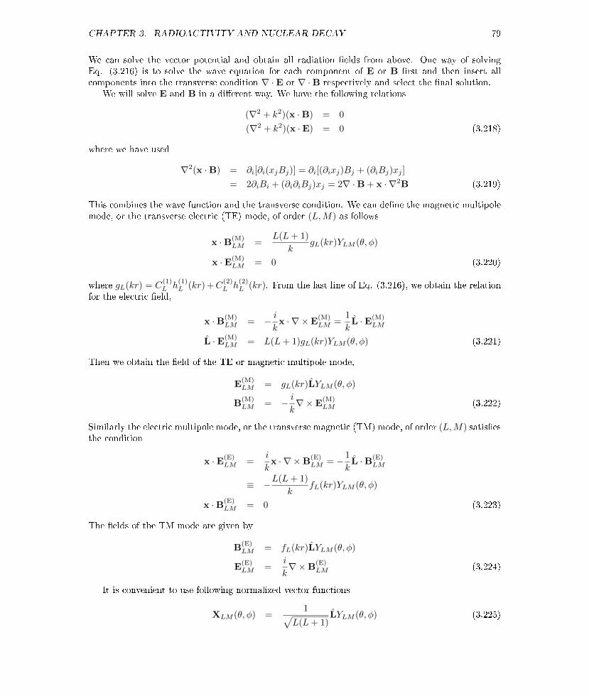
CHAPTER 3. RADIOACTIVITY AND NUCLEAR DECAY 79
We can solve the vector potential and obtain all radiation elds from above. One way of solvingEq. (3.216) is to solve the wave equation for each component of E or B rst and then insert allcomponents into the transverse condition ∇ ·E or ∇ ·B respectively and select the nal solution.
We will solve E and B in a dierent way. We have the following relations
(∇2 + k2)(x ·B) = 0
(∇2 + k2)(x ·E) = 0 (3.218)
where we have used
∇2(x ·B) = ∂i[∂i(xjBj)] = ∂i[(∂ixj)Bj + (∂iBj)xj ]
= 2∂iBi + (∂i∂iBj)xj = 2∇ ·B + x · ∇2B (3.219)
This combines the wave function and the transverse condition. We can dene the magnetic multipolemode, or the transverse electric (TE) mode, of order (L,M) as follows
x ·B(M)LM =
L(L+ 1)
kgL(kr)YLM (θ, φ)
x ·E(M)LM = 0 (3.220)
where gL(kr) = C(1)L h
(1)L (kr) +C
(2)L h
(2)L (kr). From the last line of Eq. (3.216), we obtain the relation
for the electric eld,
x ·B(M)LM = − i
kx · ∇ ×E
(M)LM =
1
kL ·E(M)
LM
L ·E(M)LM = L(L+ 1)gL(kr)YLM (θ, φ) (3.221)
Then we obtain the eld of the TE or magnetic multipole mode,
E(M)LM = gL(kr)LYLM (θ, φ)
B(M)LM = − i
k∇×E
(M)LM (3.222)
Similarly the electric multipole mode, or the transverse magnetic (TM) mode, of order (L,M) satisesthe condition
x ·E(E)LM =
i
kx · ∇ ×B
(E)LM = −1
kL ·B(E)
LM
≡ −L(L+ 1)
kfL(kr)YLM (θ, φ)
x ·B(E)LM = 0 (3.223)
The elds of the TM mode are given by
B(E)LM = fL(kr)LYLM (θ, φ)
E(E)LM =
i
k∇×B
(E)LM (3.224)
It is convenient to use following normalized vector functions
XLM (θ, φ) =1√
L(L+ 1)LYLM (θ, φ) (3.225)

CHAPTER 3. RADIOACTIVITY AND NUCLEAR DECAY 80
which satisfy the normalization and orthogonality conditions∫dΩX∗L′M ′ ·XLM = δLL′δMM ′∫
dΩX∗L′M ′ · (r×XLM ) = 0 (3.226)
So general solutions to Maxwell's equations in multipole expansion can be expressed by
E =∑L,M
[i
kc(E)(L,M)∇× fL(kr)XLM + c(M)(L,M)gL(kr)XLM
]
B =∑L,M
[c(E)(L,M)fL(kr)XLM −
i
kc(M)(L,M)∇× gL(kr)XLM
](3.227)
The vector potential can be obtained by E = −∂A/∂t = ikA,
A =∑L,M
[1
k2c(E)(L,M)∇× fL(kr)XLM −
i
kc(M)(L,M)gL(kr)XLM
]=
∑L,M
[a(E)(L,M)A(E)LM (k,x) + a(M)(L,M)A
(M)LM (k,x)] (3.228)
In Eqs. (3.227,3.228) a(E),(M) and c(E),(M) are all expansion coecients. We can verify that the abovevector potential really satises B = ∇×A. We can check this. The second term does obviously obeyB = ∇×A, so does the rst term since
∇× ∇× [fL(kr)XLM ] = ∇(∇ · [fL(kr)XLM ])−∇2[fL(kr)XLM ]
= k2fL(kr)XLM (3.229)
where we have used (∇2 + k2)[fL(kr)XLM ] = 0. We can choose fL(kr) = gL(kr) by re-dening c(E)
and c(M), then we have
A(E)LM (k,x) =
i
k∇×A
(M)LM (k,x) (3.230)
In proper nomalization, the vector potential of a TE mode is given by
A(M)LM = k
√8π
R0XLM (θ, φ)jL(kr) (3.231)
where have chosen jL(kr) for it fullls the boundary condition A(M)LM (r = 0) should be nite and
A(M)LM (r → ∞) = 0. The parity of the magnetic multipole eld is (−1)L. Due to x · L = 0, we see
that A(M)LM is perpendicular to x. The normalization constant can be determined from∫
d3xA(M)∗LM ·A(M)
L′M ′ =8πkk′
R0
∫dΩX∗LM ·XL′M ′
∫drr2jL(kr)jL′(k
′r)
= 4πδLL′δMM ′δk,k′ (3.232)
where we have assumed for kR0 > kr L,
jL(kr) ≈ 1
krsin(kr − π
2L) (3.233)
The boundary condition
jL(kR0) = 0, knR0 −π
2L = nπ (3.234)

CHAPTER 3. RADIOACTIVITY AND NUCLEAR DECAY 81
So we have
k3
∫ R0
0
drr2j2L(kr) =
∫ kR0
0
dyy2j2L(y)
≈∫ kR0
0
dy sin2(y − π
2L) =
1
2kR0 (3.235)
The the vector potential of a TM mode is obtained by Eq. (3.230),
A(E)LM (k,x) =
i
k∇×A
(M)LM (k,x) = i
√8π
R0∇×XLM (θ, φ)jL(kr)
The parity of the electric multipole eld is (−1)L+1. The TE and TM modes are dual to each other,
E(E)LM = B
(M)LM , B
(E)LM = −E
(M)LM (3.236)
The energy ows of both TE and TM modes are along x.
Having the transverse radiation elds A(E),(M)LM , we can write down the general solution by expan-
sion and quantize it,
A(t,x) =∑L,M,k
∑σ=(E),(M)
1√2ω
[aσ(k, L,M)Aσ
LM (k,x)e−iωt
+a†σ(k, L,M)Aσ∗LM (k,x)eiωt
](3.237)
where aσ and a†σ are destruction and creation operators,
[aσ(k, L,M), a†σ′(k′, L′,M ′)] = δσ,σ′δLL′δMM ′δkk′
all others = 0 (3.238)
The Hamiltonian for the radiation eld is
Hrad =1
8π
∫d3x(E2 + B2) =
1
8π
∫d3x
[(∂A
∂t
)2
+ (∇×A)2
]
=∑
L,M,k,σ
k
[a†σ(k, L,M)aσ(k, L,M) +
1
2
](3.239)
Here we treat the nucleus as a single identity. The transition amplitude from the initial state to thenal state is
λ = 2π |〈b, 1 |HI| a, 0〉|2 ρ(Ef ) (3.240)
where HI is given by Eq. (3.182). Here ρ(Ef ) is the density of nal states,
ρ(Ef ) =dn
dEf=R0
π(3.241)
where we have used Eq. (3.234).For electric multipole radiation or TM mode the non-vanishing term in the matrix element
〈b, 1 |HI | a, 0〉 comes from the creation operator term in the vector eld A(t,x) and magnetic eldB(t,x),
1√2ωa†(E)(k, L,M)A
(E)∗LM (k, r) = −ia†(E)(k, L,M)
√4π
R0ω∇× [X∗LM (θ, φ)jL(kr)]
1√2ωa†(E)(k, L,M)B
(E)∗LM (k, r) = −ia†(E)(k, L,M)
√4π
R0ω∇×∇× [X∗LM (θ, φ)jL(kr)](3.242)

CHAPTER 3. RADIOACTIVITY AND NUCLEAR DECAY 82
where
A(E)∗LM (k, r) = −i
√8π
R0∇× [X∗LM (θ, φ)jL(kr)]
B(E)∗LM (k, r) = ∇×A
(E)∗LM (k, r) (3.243)
Substituting Eq. (3.242) into HI in Eq. (3.182) and using Eq. (3.240), we obtain the amplitude forone charged particle (we suppressed the particle label in the charge and g-factor),
〈b, 1 |HI| a, 0〉 = i1
2m
√4π
R0ωL(L+ 1)
×eq⟨
b∣∣∣[∇× (L∗Y ∗LM jL)] · (−i∇) + (−i∇) · [∇× (L∗Y ∗LM jL)]
∣∣∣ a⟩+ eg
⟨b∣∣∣σ · ∇ × [∇× (L∗Y ∗LM jL)]
∣∣∣ a⟩= i
1
2m
√4π
R0ωL(L+ 1)
×eq 〈b |[∇× (x×∇Y ∗LM jL)] · ∇+∇ · [∇× (x×∇Y ∗LM jL)]| a〉+ eg
⟨b∣∣∣σ · ∇ × [∇× (L∗Y ∗LM jL)]
∣∣∣ a⟩= −i
√4π(L+ 1)
R0ωL
kL+1
(2L+ 1)!!
×eq⟨b∣∣rLY ∗LM ∣∣ a⟩+ kg
e
2m
1
L+ 1
⟨b∣∣∣[σ · L(rLY ∗LM )]
∣∣∣ a⟩
= −i√
4π(L+ 1)
R0ωL
kL+1
(2L+ 1)!!(Q1,LM +Q2,LM ) (3.244)
Here we have assumed that there is only one charged particle in the system, we will add a sum overall particles in the end. We also assume that kr is very small, i.e. the photon wavelength is muchsmaller than nucleus size. We have dened
Q1,LM = eq⟨b∣∣rLY ∗LM ∣∣ a⟩
Q2,LM = ge
2m
k
L+ 1
⟨b∣∣∣[σ · L(rLY ∗LM )]
∣∣∣ a⟩ (3.245)
We have used
ψ∗b[∇× (x×∇Y ∗LM jL)] · ∇ψa + ψ∗b∇ · [∇× (x×∇Y ∗LM jL)]ψa
= 2m(L+ 1)kL
(2L+ 1)!!ψ∗b−
∇2
2m(rLY ∗LMψa)− rLY ∗LM (−∇
2
2m)ψa
= 2m(L+ 1)kL
(2L+ 1)!!ψ∗b[−
∇2
2m+ V (r)]rLY ∗LM − rLY ∗LM [−∇
2
2m+ V (r)]ψa
= −2m(L+ 1)kL
(2L+ 1)!!(Ea − Eb)ψ∗br
LY ∗LMψa
= −2m(L+ 1)kL+1
(2L+ 1)!!ψ∗br
LY ∗LMψa (3.246)

CHAPTER 3. RADIOACTIVITY AND NUCLEAR DECAY 83
and
σ · ∇ × [∇× (L∗Y ∗LM jL)] = iσ · ∇ × [∇× (x×∇Y ∗LM jL)]
= iσ · ∇ × [x∇2(Y ∗LM jL)]
= −ik2σ · ∇ × (xY ∗LM jL) = ik2σ · [x×∇(Y ∗LM jL)]
≈ ikL+2
(2L+ 1)!!(σ × x) · ∇(rLY ∗LM )
= − kL+2
(2L+ 1)!!σ · L(rLY ∗LM ) (3.247)
Here in deriving the above two formula we have used
ψ∗b[∇× (x×∇Y ∗LM jL)] · ∇ψa + ψ∗b∇ · [∇× (x×∇Y ∗LM jL)]ψa
≈ − (L+ 1)kL
(2L+ 1)!!ψ∗b[∇(rLY ∗LM )] · ∇ψa + ψ∗b∇ · [∇(rLY ∗LM )ψa]
= − (L+ 1)kL
(2L+ 1)!!ψ∗b[∇(rLY ∗LM )] · ∇ψa + ψ∗b∇ · [∇(rLY ∗LMψa)− rLY ∗LM∇ψa]
= − (L+ 1)kL
(2L+ 1)!!ψ∗b[∇(rLY ∗LM )] · ∇ψa
+ψ∗b[∇2(rLY ∗LMψa)−∇(rLY ∗LM ) · ∇ψa − rLY ∗LM∇2ψa]
− (L+ 1)kL
(2L+ 1)!!ψ∗b∇2rLY ∗LM − rLY ∗LM∇2ψa (3.248)
and
jL(kr) ≈ (kr)L
(2L+ 1)!!, for kr 1
xj∂j∂h = ∂hxj∂j − ∂h∇× (x×∇Y ∗LM jL) = ehεhniεijk∂n(xj∂kY
∗LM jL)
= ehεhniεijk(δnj∂k + xj∂n∂k)Y ∗LM jL
= eh(δhjδnk − δhkδnj)(δnj∂k + xj∂n∂k)Y ∗LM jL
= eh(xh∂2 − 2∂h − xj∂j∂h)Y ∗LM jL
= eh[xh∂2 − ∂h(1 + xj∂j)]Y
∗LM jL
= [x∇2 −∇(1 + r∂r)]Y∗LM jL
= −xk2Y ∗LM jL − [∇(1 + r∂r)Y∗LM jL]
≈ −xk2(kr)L
(2L+ 1)!!− (L+ 1)kL
(2L+ 1)!!∇(rLY ∗LM )
≈ − (L+ 1)kL
(2L+ 1)!!∇(rLY ∗LM ) (3.249)
So the transition rate from the electric multipole eld is
λ(E) = 2π |〈b, 1 |HI | a, 0〉|2 ρ(Ef )
=8π(L+ 1)
L[(2L+ 1)!!]2k2L+1
∑Ma,Mb,M
1
2Ja + 1|Q1,LM +Q2,LM |2 (3.250)
where we have taken average over the initial states and sum over the nal states. When we recover

CHAPTER 3. RADIOACTIVITY AND NUCLEAR DECAY 84
the sum over all charged particles, Q1(2),LM are given by
Q1,LM = e∑i
qi⟨b∣∣rLi Y ∗LM (i)
∣∣ a⟩Q2,LM =
k
L+ 1
∑i
gie
2mi
⟨b∣∣∣(σi · Li)[rLi Y ∗LM (i)]
∣∣∣ a⟩ (3.251)
From spherical harmonics, Y1,±1(θ, φ) = ∓√
3/8π sin θe±iφ, Y1,0(θ, φ) =√
3/4π cos θ, we have
Q1;1,±1 = ∓√
3
8π
⟨b
∣∣∣∣∣e∑i
qi(xi ± iyi)∣∣∣∣∣ a⟩
Q1;1,0 =
√3
4π
⟨b
∣∣∣∣∣e∑i
qizi
∣∣∣∣∣ a⟩
(3.252)
If we neglect Q2,LM , Eq. (3.250) becomes
λ(E1) =4
3ω3k
∑Ma,Mb
1
2Ja + 1|Dba(Mb,Ma)|2 (3.253)
The power of radiation is then
I(E1) =4
3ω4k
∑Ma,Mb
1
2Ja + 1|Dba(Mb,Ma)|2 (3.254)
which is the same as Eq. (3.197). From Eq. (3.251) we have Q1 = Q2 = 0 when L = 0, so there isno E0 transition.
Now we consider the magnetic multipole transition. The vector potential and magnetic elds fora L,M mode which appear in the creation operator term are given by
A(M)∗LM (k, r) = k
√8π
R0X∗LM (θ, φ)jL(kr)
B(M)∗LM (k, r) = ∇×A
(M)∗LM (k, r) (3.255)
Then the creation operator terms in A(t,x) and magnetic eld B(t,x) are given by
1√2ωa†(M)(k, L,M)A
(M)∗LM (k, r) = a†(M)(k, L,M)
√4π
R0ωX∗LM (θ, φ)jL(kr)
1√2ωa†(M)(k, L,M)B
(M)∗LM (k, r) = a†(M)(k, L,M)
√4π
R0ω∇× [X∗LM (θ, φ)jL(kr)] (3.256)
CHAPTER 3. RADIOACTIVITY AND NUCLEAR DECAY 85
Substituting the above into Eq. (3.240), we get the transition amplitude,
〈b, 1 |HI| a, 0〉 = − k
2m
√4π
R0ωL(L+ 1)
×eq⟨
b∣∣∣(L∗Y ∗LM jL) · (−i∇) + (−i∇) · (L∗Y ∗LM jL)
∣∣∣ a⟩+ eg
⟨b∣∣∣σ · [∇× (L∗Y ∗LM jL)]
∣∣∣ a⟩= − k
2m
√4π
R0ωL(L+ 1)
×eq 〈b |(x×∇Y ∗LM jL) · ∇+∇ · (x×∇Y ∗LM jL)| a〉+ eg
⟨b∣∣∣σ · [∇× (L∗Y ∗LM jL)]
∣∣∣ a⟩= − k
2m
√4π
R0ωL(L+ 1)
kL
(2L+ 1)!!
×−2ieq
⟨b∣∣∣L · ∇(rLY ∗LM )
∣∣∣ a⟩− ieg(L+ 1)⟨b∣∣σ · ∇(rLY ∗LM )
∣∣ a⟩= i
√4π(L+ 1)
R0ωL
kL+1
(2L+ 1)!!(M1,LM +M2,LM ) (3.257)
Here we have used
ψ∗b(x×∇Y ∗LM jL) · ∇ψa + ψ∗b∇ · (x×∇Y ∗LM jL)ψa
= 2ψ∗b(x×∇Y ∗LM jL) · ∇ψa = −2ψ∗b(∇Y ∗LM jL) · (x×∇ψa)
= 2ψ∗b∇ · (x×∇Y ∗LM jL)ψa
= −2ψ∗bx×∇ · [∇(Y ∗LM jL)ψa] (3.258)
σ · [∇× (L∗Y ∗LM jL)] = iσ · ∇ × [x×∇(Y ∗LM jL)]
≈ −i (L+ 1)kL
(2L+ 1)!!σ · ∇(rLY ∗LM ) (3.259)
The transition rate from the magnetic multipole eld or TE mode is
λ(M) =8π(L+ 1)
L[(2L+ 1)!!]2k2L+1
∑Ma,Mb,M
1
2Ja + 1|M1,LM +M2,LM |2 (3.260)
where M1,LM and M2,LM are dened by
M1,LM =1
L+ 1
∑i
eqimi
⟨b∣∣∣Li · ∇i[rLi Y ∗LM (i)]
∣∣∣ a⟩=
1
L+ 1
∑i
eqimi
⟨b∣∣∣∇i[rLi Y ∗LM (i)] · Li
∣∣∣ a⟩M2,LM =
∑i
gie
2mi
⟨b∣∣σi · ∇i[rLi Y ∗LM (i)]
∣∣ a⟩ (3.261)
where we have recovered the sum over all charged particles. From Eq. (3.261) we have M1 = M2 = 0for L = 0, so there is no M0 transition.
Let us estimate the magnitude of the transition. For the electric multipole eld,
Q1,LM = eq⟨b∣∣rLY ∗LM ∣∣ a⟩ ∼ e ⟨rL⟩ ∼ e∫ drrL+2∫
drr2∼ e 3
L+ 3RL
Q2,LM = ge
2m
k
L+ 1
⟨b∣∣∣(σ · L)(rLY ∗LM )
∣∣∣ a⟩ ∼ eω
m
3
2(L+ 1)(L+ 3)RL (3.262)

CHAPTER 3. RADIOACTIVITY AND NUCLEAR DECAY 86
For the nuclear γ decay, the ratio becomes
Q2,LM
Q1,LM∼ ω
m∼ 10−3 (3.263)
So we can neglect Q2,LM relative to Q1,LM . For the magnetic multipole eld, M1,LM and M2,LM areof the same order,
M1,LM ∼ M2,LM ∼e
mRL−1 (3.264)
The transitions of the higher order are much suppressed relative to the lower order,
λ(E)(L+ 1)
λ(E)(L)∼ λ(M)(L+ 1)
λ(M)(L)∼ k2R2 ∼ (MeV · 10 fm)2 ∼ 2.5× 10⁻³ (3.265)
The magnitude of the magnetic transition is suppressed relative to that of electric one of the sameorder,
λ(M)(L)
λ(E)(L)∼ 1
m2R2∼ 1
(1 GeV · 10 fm)2∼ 4× 10⁻⁴ (3.266)
Then we can roughly have the relation λ(E)(L + 1) ∼ λ(M)(L), i.e. E(L+1) radiation is comparableto ML one in magnitude.
Selection rules for parity are given as follows. The parity of the operators are know as
P (rLY ∗LM ) = (−1)L
P [L · ∇(rLY ∗LM )] = P [σ · ∇(rLY ∗LM )] = (−1)L−1 (3.267)
For EL and ML transitions
PiPf = (−1)L, EL
PiPf = (−1)L+1, ML (3.268)
where Pi,f are parities for the initial and nal states.Selection rules for angular momentum. Following the Wigner-Eckart theorem,
〈Jf ,Mf |TLM | Ji,Mi〉 = CJfMf
JiMi,LM〈Jf ‖TLM‖ Ji〉 (3.269)
where
TLM = rLY ∗LM , L · ∇(rLY ∗LM ), σ · ∇(rLY ∗LM ) (3.270)
and L 6= 0 obeys that Jf ,Ji,L form a vector triangle,
Jf = Ji + L
|Ji − Jf | ≤ L ≤ |Ji + Jf | (3.271)
There is no transition with Ji = Jf and L = 0 since there is no monopole transition. Note that thetransition with L = |Ji − Jf | is dominant.
The mixing only takes place between E(2L) and E(2L'), M(2L) and M(2L') or ML and E(L+1)[but not EL and M(L+1) due to the disparity of the two transition strengths]. For example, atransition 2+ → 1+ can be M1 or E2. From the parity conservation (−1)L/(−1)L+1 must be 1 forelectric/magnetic eld, so Lmust be even/odd for the electric/magnetic eld. For angular momentumconservation, we have L = 1, 2, 3. So the possible transitions are M1, E2 or M3. The dominanttransitions are M1 or E2.

CHAPTER 3. RADIOACTIVITY AND NUCLEAR DECAY 87
Table 3.4: Selection rules for parity and angular momentum. Note that when
|Ji − Jf | 0,1 2 3 4 5PiPf = + M1(E2) E2 M3(E4) E4 M5(E6)PiPf = − E1 M2(E3) E3 M4(E5) E5
Figure 3.23: Energy spectra of electrons from beta decay and internal conversion of radioactive nuclei.The peaks on top of continuous the spectrum are from internal conversion.
N_e
T_e
X−ray
e^−

CHAPTER 3. RADIOACTIVITY AND NUCLEAR DECAY 88
Figure 3.24: The electron spectrum in the β-decay 203Hg→203 Tl with internal conversion of 203Tl.

CHAPTER 3. RADIOACTIVITY AND NUCLEAR DECAY 89
There are no 0+ → 0+ transition, since this would need a monopole radiation with L = 0 whichdoes not exist. These decay processed can happen through internal conversion. Internal conversion isa radioactive decay where a transition of an excited nucleus to its lower energy level takes place and theenergy is transfered to an electron on the inner atomic shell which is kicked out. Internal conversionis not photo-electric eect since there is no photon involved. The electrons emitted from internalconversion can be distinguished from those from the β-decay. The electron energy is continuous inthe β-decay, while it is discrete in the internal conversion. See Fig. 3.23.
The electron energy in internal conversion can be expressed by Te = Eγ −W , where Eγ is thetransition energy and W is the binding energy of the electron in the atomic shell. Normally anelectron in the K-shell (n = 1) is kicked out, so from the K-shell binding energy WK and the electronenergy Te we can determine the transition energy or the dierence of the two energy levels. For theL-shell (n = 2) electrons, there are atomic orbitals 2s1/2, 2p1/2 and 2p3/2, which are also called LI ,LII and LIII shells. The vacancy left by the knocked out electron is instantly lled by the electronfrom an outer shell. This results in accompanying X-ray.
As an example we consider the β decay of 20380 Hg→203
81 Tl followed by a γ-decay of energy 279.19keV. We need to know the electron binding energies of the Tl (Thallium) atom whose lower shells are[4],
B(K) = 85.529 keV
B(LI) = 15.347 keV
B(LII) = 14.698 keV
B(LIII) = 12.657 keV
B(MI) = 3.704 keV (3.272)
So the conversion electrons have energies as follows,
Te(K) = (279.19− 85.529) keV = 193.661 keV
Te(LI) = (279.19− 15.347) keV = 263.843 keV
Te(LII) = (279.19− 14.698) keV = 264.492 keV
Te(LIII) = (279.19− 12.657) keV = 266.533 keV
Te(MI) = (279.19− 3.704) keV = 275.486 keV (3.273)
See Fig. 3.24 for the electron spectrum of 203Hg. One can see the peaks on the continuous backgroundof the β-decay. The intensities of internal conversion varies from β decays. In some cases internalconversion is favored over the γ emission, in others, it is opposite. We can dene the ratio of theinternal conversion rate (decay constant) to the γ-emission rate, α = λe/λγ . Then the total decayconstant can be put in the form λt = λγ(1 + α).
Let us take the γ-emission of Se-72 for an example. The enegry level of Se-72 is shown in Fig.3.25. We notice that the 937-MeV transition must be an internal conversion since it is a 0+ → 0+
transition. Let us look at the energy level of 1317 keV. The half life of the level 1317 keV is 8.7 ps,whose total decay rate is
λt =ln 2
t1/2=
0.693
8.7× 10⁻¹²s= 7.97× 10¹⁰ s−1 (3.274)
The total decay rate is the sum of the rates for three transitions, 1317 keV, 455 keV and 380 keV,
λt = λ1317 + λ455 + λ380
= λγ,1317(1 + α1317) + λγ,455(1 + α455) + λγ,380(1 + α380)
≈ λγ,1317 + λγ,455 + λγ,380 (3.275)
The relative intensities for these γ-decays are
λγ,1317 : λγ,455 : λγ,380 = 51 : 39 : 10 (3.276)
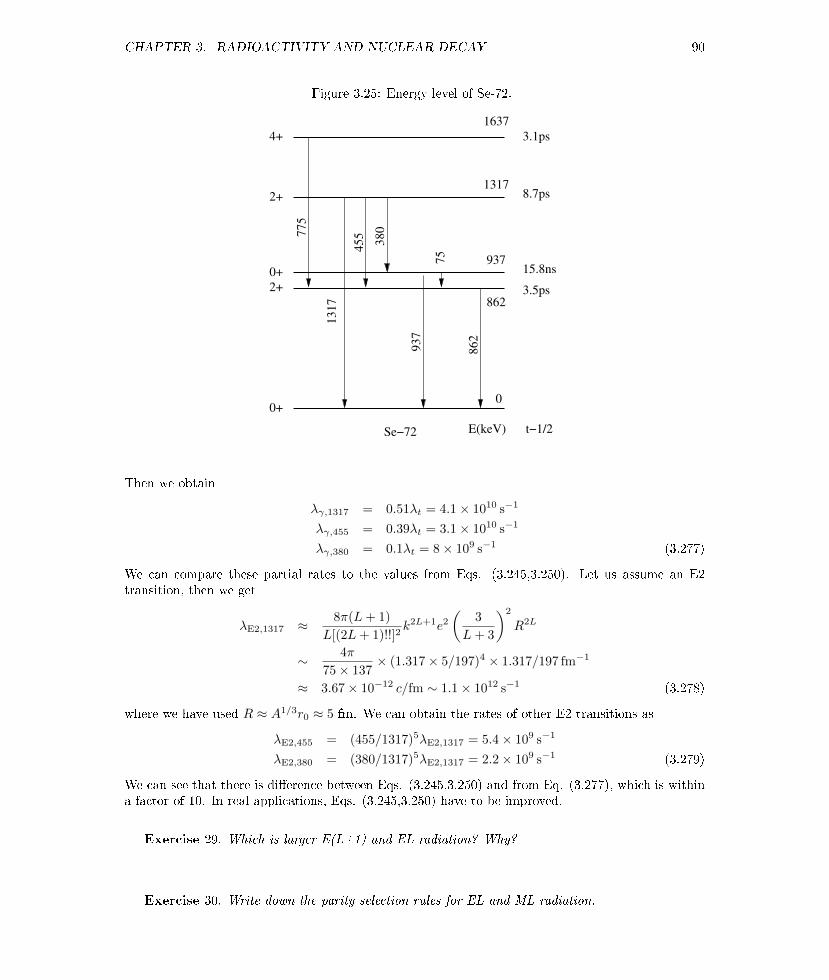
CHAPTER 3. RADIOACTIVITY AND NUCLEAR DECAY 90
Figure 3.25: Energy level of Se-72.
1637
1317
937
862
0
E(keV) t−1/2
3.1ps
8.7ps
15.8ns
3.5ps
Se−72
4+
2+
0+
2+
0+
775
1317
455
380
937
862
75
Then we obtain
λγ,1317 = 0.51λt = 4.1× 10¹⁰ s−1
λγ,455 = 0.39λt = 3.1× 10¹⁰ s−1
λγ,380 = 0.1λt = 8× 10⁹ s−1 (3.277)
We can compare these partial rates to the values from Eqs. (3.245,3.250). Let us assume an E2transition, then we get
λE2,1317 ≈ 8π(L+ 1)
L[(2L+ 1)!!]2k2L+1e2
(3
L+ 3
)2
R2L
∼ 4π
75× 137× (1.317× 5/197)4 × 1.317/197 fm−1
≈ 3.67× 10⁻¹² c/fm ∼ 1.1× 10¹² s−1 (3.278)
where we have used R ≈ A1/3r0 ≈ 5 fm. We can obtain the rates of other E2 transitions as
λE2,455 = (455/1317)5λE2,1317 = 5.4× 10⁹ s−1
λE2,380 = (380/1317)5λE2,1317 = 2.2× 10⁹ s−1 (3.279)
We can see that there is dierence between Eqs. (3.245,3.250) and from Eq. (3.277), which is withina factor of 10. In real applications, Eqs. (3.245,3.250) have to be improved.
Exercise 29. Which is larger E(L+1) and EL radiation? Why?
Exercise 30. Write down the parity selection rules for EL and ML radiation.

CHAPTER 3. RADIOACTIVITY AND NUCLEAR DECAY 91
Figure 3.26: The Mössbauer eect: recoil-free nuclear resonance emission and absorption of gamma-ray.
excited state excited state
ground stateground state
absorbersource
γ
absorption spectra
Exercise 31. For the γ-decay from the transition 2+ → 1− , what are the possible types ofmultipole radiations? why?
Exercise 32. The ratio of the transition rate of E(L+1) to EL and M(L+1) to ML transitioncan be estimated as
r1 =λ(E)(L+ 1)
λ(E)(L)∼ λ(M)(L+ 1)
λ(M)(L)∼ k2R2
where k is the wave number (momentum) of the Gamma ray and R is the typical radiusof the nucleus. The ratio of the transition rate of magnetic to electric transition can beestimated as
r2 =λ(M)(L)
λ(E)(L)∼ 1
m2R2
where m is the nucleon mass. (1) Try to estimate r1 and r2 for typical values of k = 1 MeVand R = 10 fm. (2) Given the initial and nal state's parities Pi and Pf for Gamma decay,write down the parity selection rule for EL and ML transition. (3) What is the angularselection rule for the Gamma decay? (4) 167
68 Er has the following energy levels starting fromthe ground state,
7
2
+
,3
2
+
,1
2
−,
3
2
−,
5
2
−
give the dominant Gamma transitions for each excited states.
3.6 Mössbauer eect
Mössbauer discovered the recoil-free emission and absorption of gamma rays by nuclei in 1958 andwas awarded the Nobel prize in physics for this eect name after him. See Fig. 3.26. Using theMössbauer eect one can make very high precision measurement of the energy to observe the nestructure.
The transition rate of an energy level is inversely proportional to its life and proportional to its

CHAPTER 3. RADIOACTIVITY AND NUCLEAR DECAY 92
width. In the γ decay, the ratio of its width to its energy is normally 10−8, which requires very highprecision measurement. One usually measure the width of a γ transition by the resonant absorption.This emission and subsequent absorption is called resonant uorescence. But the recoil of the mothernuclei will take o a lot of energy making the resonant absorption very dicult. Mössbauer was therst physicist who tackled this diculty.
Take the gamma decay 14.4 KeV of 5726Fe∗ as example. The momentum of the photon is
p ≡ |p| = 0.0144 MeV (3.280)
The recoil energy of the nucleus is
ER =p2
2m=
(0.0144)2
2× 57× 931≈ 2× 10⁻³ eV (3.281)
The lifetime of the excited state of 5726Fe∗ is τ ∼ 10−7s. The width of 57
26Fe∗ is then
Γ =1
τ≈ 1
10−7 × 3× 108 × 1015fm−1 ≈ 3.3× 10⁻¹⁷ fm−1
≈ 197× 3.3× 10−17 MeV ≈ 6× 10⁻⁹ eV (3.282)
One seesER Γ (3.283)
In this case the resonant absorption cannot take place. For the resonant absorption to occur, oneshould have
Eγ,em = E0 − EREγ,ab = E0 + ER
Eγ,ab − Eγ,em = 2ER < 2Γ (3.284)
It was a great breakthrough to realize that one could get resonance absorption of gamma rays byputting the source nuclei in a crystal in low temperature. To see how many iron nuclei would haveto recoil together to keep the gamma within the natural linewidth:
ER =p2
2mN= Γ,
N =p2
2mΓ≈ 2× 10⁻³
6× 10⁻⁹≈ 3.3× 10⁵ (3.285)
which is many orders of magnitude smaller than the macroscopic scale 1023.
Exercise 33. The resonant absorption without recoil is observed in the γ-decay of 19177 Ir114.
The energy of the photon is 120 KeV and the width of the spectrum is given by its lifeτ ≈ 1.4 × 10⁻¹⁰ s. Estimate the recoil energy of the nucleus if the nucleus is put in freespace. In order for the resonant absorption to take place, what is the least mass of the crystalin which the nuclei are embeded in order for the resonant absorption to take place.
Chapter 4
Nuclear models
A nucleus is a many body system of nucleons. Nucleons interact with each other via nuclear force.Besides two-body forces, there are many-body forces like three-body forces etc.. Nuclear models aresimplied descriptions of some of nuclear properties.
4.1 The shell model
4.1.1 Phenomena related to shell structure
It is found that a nucleus is stable when the neutron or proton number is 2,8,20,28,50,82, and theneutron number is 126. These numbers are called the magic numbers. A nucleus can be singly magicwith proton or neutron number being a magic number, or doubly magic with both proton and neutronnumbers being magic numbers. Several evidences about the magic numbers are as follows.
(1) Abundance. (a) On the earth, the following nuclei are more abundant than their neighbors:
42He2,
168 O8,
4020Ca20,
6028Ni32,
8838Sr50,
9040Zr50,
12050 Sn70,
12856 Ba82,
14058 Ce82,
20882 Pb126 (4.1)
In nuclei with even proton numbers (even Z), it is less likely that their abundances are more than50%. There are exceptions: the abundances of 88
38Sr50,13856 Ba82 and 140
58 Ce82 are 82.56%, 71.66% and88.48%. One can see that when the neutron number is 50 or 82 the nucleus is much more stable thana normal one. (b) In all stable elements, those with neutron number 20, 28, 50, 82 have more numberof isotones than their neighbors. Elements with N = 20, 28 have 5 isotones, N = 50 have 6, N = 82have 7. (c) When the proton number Z = 8, 20, 28, 50, 82, the number of stable isotopes are muchlarger than their neighbors. (d) The presence of pairing energy shows that even-even nuclei are morestable than odd-odd ones, see Table 2.2. (e) The average excitation energy of the rst excited statein even-even nuclei show a maximum when the neutron number is a magic one.
(2) The binding or separation energies of the last nucleon for nuclei are dened by
Sn = B(Z,A)−B(Z,A− 1) = M(Z,A− 1)−M(Z,A) +mn
Sp = B(Z,A)−B(Z − 1, A− 1) = M(Z − 1, A− 1)−M(Z,A) +mp (4.2)
They are much smaller for nuclei with Z − 1 or N − 1 being magic numbers than others, whichindicates that the nuclei with magic number are more tightly bound. The neutron binding energy issmall for nuclei with N = 8, 20, impling that it is relatively hard for them to capture a neutron. Theempirical formula for the nuclear binding energy per nucleon deviates from data strongly when N orZ are magic numbers. The neutron capture cross sections are much smaller for nuclei whose neutronnumbers are magic numbers. See Fig. 4.1.
(3) There are sudden changes of nucleus radius for nuclei whose neutron numbers are magicnumbers.
93
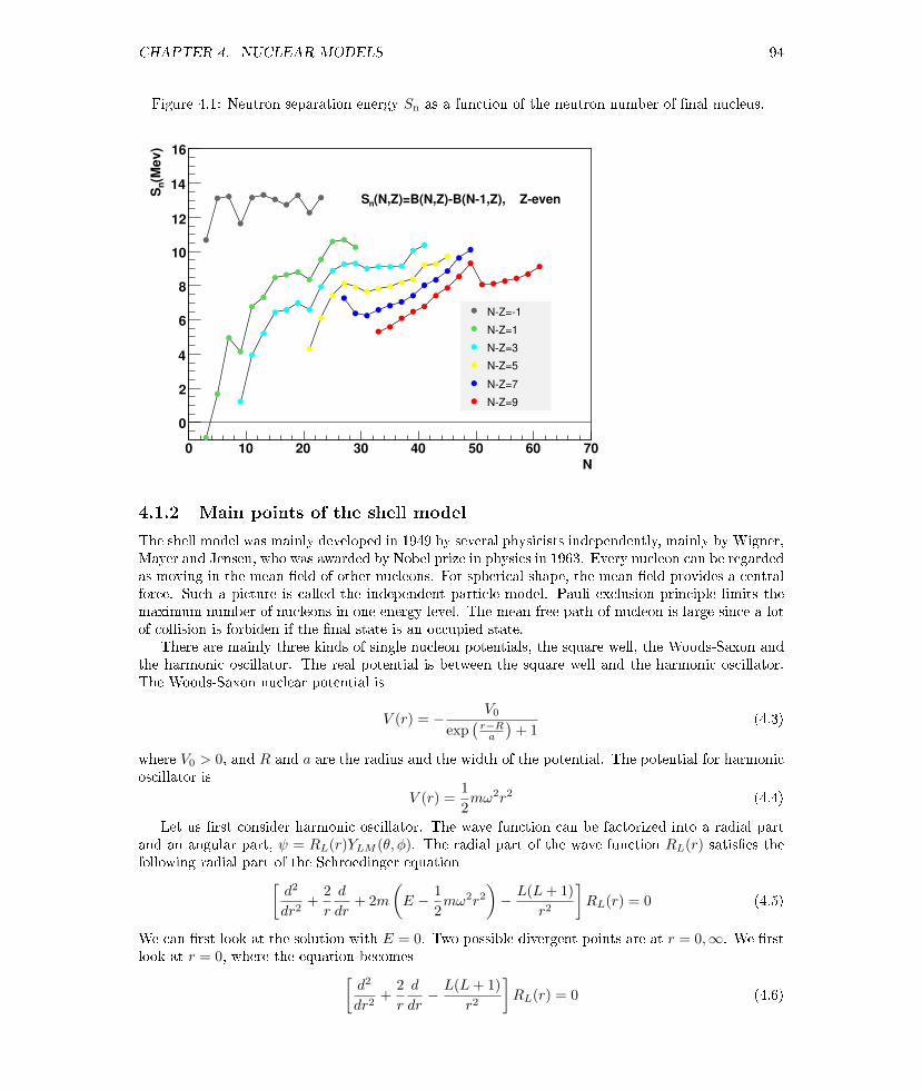
CHAPTER 4. NUCLEAR MODELS 94
Figure 4.1: Neutron separation energy Sn as a function of the neutron number of nal nucleus.
N
0 10 20 30 40 50 60 70
(Mev)
nS
0
2
4
6
8
10
12
14
16
N-Z=-1
N-Z=1
N-Z=3
N-Z=5
N-Z=7
N-Z=9
(N,Z)=B(N,Z)-B(N-1,Z), Z-evennS
4.1.2 Main points of the shell model
The shell model was mainly developed in 1949 by several physicists independently, mainly by Wigner,Mayer and Jensen, who was awarded by Nobel prize in physics in 1963. Every nucleon can be regardedas moving in the mean eld of other nucleons. For spherical shape, the mean eld provides a centralforce. Such a picture is called the independent particle model. Pauli exclusion principle limits themaximum number of nucleons in one energy level. The mean free path of nucleon is large since a lotof collision is forbiden if the nal state is an occupied state.
There are mainly three kinds of single nucleon potentials, the square well, the Woods-Saxon andthe harmonic oscillator. The real potential is between the square well and the harmonic oscillator.The Woods-Saxon nuclear potential is
V (r) = − V0
exp(r−Ra
)+ 1
(4.3)
where V0 > 0, and R and a are the radius and the width of the potential. The potential for harmonicoscillator is
V (r) =1
2mω2r2 (4.4)
Let us rst consider harmonic oscillator. The wave function can be factorized into a radial partand an angular part, ψ = RL(r)YLM (θ, φ). The radial part of the wave function RL(r) satises thefollowing radial part of the Schroedinger equation[
d2
dr2+
2
r
d
dr+ 2m
(E − 1
2mω2r2
)− L(L+ 1)
r2
]RL(r) = 0 (4.5)
We can rst look at the solution with E = 0. Two possible divergent points are at r = 0,∞. We rstlook at r = 0, where the equation becomes[
d2
dr2+
2
r
d
dr− L(L+ 1)
r2
]RL(r) = 0 (4.6)

CHAPTER 4. NUCLEAR MODELS 95
which has two solutions,
RL ∼ rL,1
rL+1(4.7)
The solution is RL ∼ rL is physical. Then we look at the case for r =∞,(d2
dr2−m2ω2r2
)Rl(r) = 0 (4.8)
The solutions areRL(r) ∼ exp(±mωr2/2) (4.9)
where we only the solution with the minus sign is physical at innity. So we can assume a generalsolution RL(r) for non-vanishing E has the following form
RL(r) ∼ rL exp(−mωr2/2)uL(r) (4.10)
Changing the variable r to a dimensionless ξ = mωr2, we arrive at the equation for the conuenthypergeometric function for uL(ξ),
ξd2uLdξ2
+
[(L+
3
2
)− ξ]duLdξ−(L+ 3/2
2− E
2ω
)uL = 0 (4.11)
whose physical solution is
u(r) ∼ F (−nr, L+3
2, ξ) (4.12)
with the radial quntum number nr given by
nr =E
2ω− L+ 3/2
2
The wave functions of a harmonic oscillator can be written in a compact and analytic form,
ψnrLM (r, θ, φ) = RnrL(r)YLM (θ, φ)
RnrL(r) = α3/2
[2L+2−nr (2L+ 2nr + 1)!!√
πnr![(2L+ 1)!!]2
]1/2
×(αr)L exp
(−1
2α2r2
)F (−nr, L+ 3/2, α2r2) (4.13)
where F is the conuent hypergeometrical function and α ≡ √mω. The energy level is,
E = (N + 3/2)ω
N = 2nr + L (4.14)
Some lowest levels and their quantum numbers are illustrated in Fig. 4.1. The degeneracy for theenergy level N is
dN = 2
[N/2]∑nr=0
[2(N − 2nr) + 1]
= (N + 1)(N + 2) (4.15)
where we have included two spin states of nucleons.Another example is the square well with depth −V0 in the range r ∈ [0, R]. The Schoedinger
equation for the radial part becomes the equation for spherical Bessel functions,[d2
dr2+
2
r
d
dr+ k2 − L(L+ 1)
r2
]RL(r) = 0 (4.16)

CHAPTER 4. NUCLEAR MODELS 96
Table 4.1: Some energy levels of the harmonic oscillator. The quantum numbers for the orbitalangular momentum are L = 0(s), 1(p), 2(d), 3(f), 4(g), 5(h).EnrL(ω) nr state nucleon accumulation(N) (nr, L) number number0 0 0s 2 21 0 0p 6 82 0,1 1s, 0d 12 203 0,1 1p, 0f 20 404 0,1,2 2s, 1d, 0g 30 705 0,1,2 2p, 1f, 0h 42 1126 0,1,2,3 3s, 2d, 1g, 0i 56 168
Table 4.2: The energy levels of the square well potential. Here n denotes the n-th zero point ofJl+1/2(x).
nL xnL dn∑n dn
1s 3.1416 2 21p 4.4934 6 81d 5.7635 10 182s 6.2832 2 201f 6.9879 14 342p 7.7253 6 401g 8.1826 18 582d 9.0950 10 681h 9.3558 22 903s 9.4248 2 92
CHAPTER 4. NUCLEAR MODELS 97
where k =√
2m(E + V0) with energy E < 0. Assuming RL = uL/√r, the above equation becomes,[
d2
dr2+
1
r
d
dr+ k2 − (L+ 1/2)2
r2
]uL(r) = 0 (4.17)
The solution which satises the boundary condition is
RL = CjL(kr)
RL|r=0 = finite
RL|r=R = CjL(kR) = 0, (4.18)
where jL(x) =√π/(2x)JL+1/2(x) is the spherical Bessel function. The wave vectors k at zero points
are denoted as knL = xnL/R, where xnL is the n-th zero point of jL(x). The energy is then
EnL = −V0 +x2nL
2mR2(4.19)
The degeneracy factor isdn = 2L+ 1 (4.20)
When applying to a nucleon system, one has to include two spin states in dn. See Table 4.2 for theenergy levels of the square well potential.
We consider a charged particle with magnetic moment moving in a magnetic eld. In the restframe of the moving particle, the interaction energy is
∆H = −µ ·B′ (4.21)
with magnetic moment µ = gq2mS. Here the magnetic eld B′ is related to B in the lab frame by
B′ = B− v ×E (4.22)
where E is the electric eld in the lab frame felt by the moving particle. In the central potential wehave
qE = −r
r
dV (r)
dr(4.23)
Then the interaction becomes
∆H = − gq
2mS ·B +
g
2m2(S · L)
1
r
dV (r)
dr(4.24)
where L = m(r × v) is the orbital angular momentum. The second term is just the spin-orbitalcoupling. Actually one can show that the spin-orbital coupling arises from the meson exchange inthe nuclear potential.
Mayer and Jensen introduced the spin-orbital coupling to nuclei for a nucleon moving in the meaneld of other nucleons,
∆V (r) = −CL · S = −C2
[(L + S)2 − L2 − S2
]= −C
2
[J(J + 1)− L(L+ 1)− 3
4
]=
−C2 L, J = L+ 1/2
C2 (L+ 1), J = L− 1/2
(4.25)
One sees that there is splitting between the levels with J = L + 1/2 and J = L − 1/2. The energylevel can be labeled by (nr, L, J).

CHAPTER 4. NUCLEAR MODELS 98
Figure 4.2: Nuclear shell model versus atomic shell model. For 3-d harmonic oscillator the energyeigenvalue is controlled by N = 2nr+ l and while for hydrogen atom it is controlled by N = nr+ l+1.The energy levels for nuclei are labeled by (nr, l, j) (left panel) or (nr + 1, l, j) (right panel). The 3-dharmonic oscillator and hydrogen atom are labeled by (nr, l).

CHAPTER 4. NUCLEAR MODELS 99
The applications of the Mayer-Jensen shell models are given in following examples.(1) The spins and parities (JP ) of the nuclei in ground states can be explained by the model. For
even-even nuclei, JP = 0+. Following the Racah seniority principle a pair of identical particles arein the lowest energy if their coupling angluar momentum is zero. This is because the wave functionshave largest overlap if the total angluar momentum is zero. For even-even nuclei every two protonsor neutrons pair, so that the total angluar momentum is vanishing. The JP of even-odd nuclei aredetermined by the unpaired nucleon. For example, the JP of 13
6 C and 137 N are (1/2)−, the spin and
parity are determined by the nucleon outside the fully occupied shell. Another example, an even-oddnucleus Niobium, 93
41Nb52, there are two neutrons outside the full shell (50) which are in the 0g7/2
state. But their pair has J = 0. The spin of the nucleus is determined by the 41-th proton which isin the 0g9/2 state. So the spin and parity of 93
41Nb52 are (9/2)+.(2) The shell model can explain the JP of nuclei of the lowest excited states. An excited state
with the lled shell plus or minus one nucleon shows single particle property and its JP is given bythat of the nucleon outside the shell.
(3) The magnetic moments of nuclei can be described by the shell model. The magnetic moment ofan odd-A nucleus is determined by the last unpaired nucleon. The magnetic moment of the unpairednucleon is
µJ = µL + µS = gLL + gSS = gJJ (4.26)
where J, L and S are the total, orbital and spin momenta. gi=J,L,S are their g-factors. We have
gJJ · J = gLL · J + gSS · J
gJJ = gLJ(J + 1) + L(L+ 1)− S(S + 1)
2(J + 1)+ gS
J(J + 1) + S(S + 1)− L(L+ 1)
2(J + 1)(4.27)
For an odd-A nucleus, its magnetic moment µJ is
µJ = gJJ = gLJ(J + 1) + L(L+ 1)− S(S + 1)
2(J + 1)+ gS
J(J + 1) + S(S + 1)− L(L+ 1)
2(J + 1)
=
gL(J − 1/2) + gS/2, J = L+ 1/2
[J/(J + 1)][gL(J + 3/2)− gS/2], J = L− 1/2(4.28)
For an odd-N and even-Z nucleus, the last nucleon is a neutron which has gL = 0 and gS = −3.82,
µJ =
−1.91, J = L+ 1/21.91 J
J+1 , J = L− 1/2(4.29)
For an even-N and odd-Z nucleus, the last nucleon is a proton which has gL = 1 and gS = 5.58,
µJ =
J + 2.29, J = L+ 1/2J − 2.29 J
J+1 , J = L− 1/2(4.30)
The experiments partially verify the above behavior for odd-A nuclei.(4) Electric quadrupole moments. The electric quadrupole moment of a nucleus is dened by
Q =1
e
∫d3r(3z2 − r2)ρe(r) =
q
e
(2⟨z2⟩−⟨x2⟩−⟨y2⟩)
(4.31)
where ρe(r) is the electric charge density and q =∫d3rρe(r) the total charge. If the charge distribution
is spherical, Q = 0. For long/short ellipsoid, Q > 0 and Q < 0. Following the shell model, the electricquadruple moment is determined by the protons outside the lled shell. For odd-Z and even-Nnucleus, there are np protons outside the lled shell and have angular momentum J , the quadruplemomemt is given by
Q = −⟨r2⟩ 2J − 1
2(J + 1)
[1− 2(np − 1)
2J − 1
](4.32)

CHAPTER 4. NUCLEAR MODELS 100
We see that when np < J + 1/2, i.e. the number of protons is less than half the number of levels,Q < 0, otherwise Q > 0. So for an odd-A nucleus with number of protons being a magic number ±1,we have Q < 0/Q > 0. The shell model can well describe the electric quadrupole moments with onlya few protons away from the magic numbers, but it can not describe those of other nuclei.
Exercise 34. For a square well potential with depth V (r) = −V0 for r ∈ [0, R] and V (r) = 0for r > R. Calculate the lowest 15 energy levels.
Exercise 35. The magnetic moments of an odd-A nucleus is determined by the last unpairednucleon. Write down its formula with respect to the nuclear spin J .
Exercise 36. Give JP of 13C, 13N and 9341Nb52.
Exercise 37. The electric quadruple moment of a nucleus is given by
Q =1
e
∫d3rρe(3z
2 − r2) =q
e
(2⟨z2⟩−⟨x2⟩−⟨y2⟩)
For an ellipsoid which is symmetric with respect to rotation along the z-axis (symmetric forx and y coordinates), give a simple explanation why Q > 0 and Q < 0 correspond to thelong and short ellipsoid.
Exercise 38. The ground states of nuclei can be treated as a many body system of identicalfermions where protons and neutrons are isospin doublets. A nucleon is moving in the meaneld of other nucleons. As a simple model, people use harmonic oscillator to simulate themean eld potential. Then nucleons ll in the single particle energy levels. The eigen-energyreads,
EN = Nω = (2nr + L)ω
For a xed N or eigen-energy, (1) calculate the degeneracy of the states, or how many statesare there having the same energy; (2) write down the states in terms of (nr + 1)L for N = 3using the notation s, p, d, f, g, h and i for L = 0, 1, 2, 3, 4, 5, 6. For example, 1s or 2fetc.. (3) When the number of protons or neutrons is the magic number 2, 8, 20, 28, 50, 82,and 126, the nuclei are most stable. But the harmonic spectra can only reproduce the rstthree magic numbers corresponding to N = 0, 1, 2. In order to explain all magic numbers,Mayer and Jensen introduced the coupling −CL · S. How to explain the magic number 28and 50? (4) The introduction of the L ·S coupling term shift the energy level for J = L+1/2and J = L − 1/2. What the energy dierence between the two levels? Which one is shiftedhigher? (5) As an application of the shell model, what's the spin and parity of 13C and13N?

CHAPTER 4. NUCLEAR MODELS 101
4.2 Collective models
For even-even nuclei, to form an excited state, it will cost much more energy to break a pair ofnucleons and excite one nucleon to higher level than in collective motion. There are three groups ofnuclei. (1) One group is around the double magic number which can be described by the shell model.This is called single particle energy levels. (2) Even-even nuclei far away from magic numbers with(60 < A < 150 or 190 < A < 220) whose lower excitations show the harmonic oscillation feature. (3)Even-even nuclei far away from magic numbers with (150 < A < 190 or A > 220) whose energy levelsare like spectra of rotation.
The shape of nuclei with double magic numbers is sphere. With increase of nucleons outside thelled shell, the shape gradually turns into ellipsoid. See Fig. 4.3. This arises from the lling ofnucleons in the energy state above the full shell in such a way that makes the binding energy larger.The nuclear deformation can be described by a mulipole expansion of a position on the nuclear surface
R(θ, φ) = R0
[1 +
∑LM
αLMYLM (θ, φ)
](4.33)
where αLM are coecents characterizing the magnitudes of the deformation. Since Y ∗LM (θ, φ) =(−1)MYL,L−M (θ, φ), the coecients satisfy α∗LM = (−1)MαL,L−M . We can remove the L = 0 term,which corresponds to the volume change. The dipole component with L = 1 of an nucleus correspondsto displacement of nucleus, which has nothing to do with internal motion of nucleons. The lowest non-vanishing component deviating from sphere is the quadupole deformation with L = 2. A deformednuclei have non-zero electric quadrupole moments.
We now look at the lowest deformation, the quadrupole with L = 2. We now list sphericalharmonic functions Y2M (θ, φ) with M = −2,−1, 0, 1, 2 as follows
Y20(θ, φ) =1
2
√5
4π(3 cos2 θ − 1),
Y2,±1(θ, φ) = ∓√
15
8πsin θ cos θe±iϕ,
Y2,±2(θ, φ) =1
2
√15
8πsin2 θe±2iϕ. (4.34)
We dene a unit vector n = (sin θ cosϕ, sin θ sinϕ, cos θ) and Y2M (θ, φ) can be rewritten as
Y20 =1
2
√5
4π(2n2
z − n2x − n2
y),
Y2,±1 = ∓√
15
8πnz(nx ± iny),
Y2,±2 =1
2
√15
8π(n2x − n2
y ± i2nxny). (4.35)
So we see that (a) α20 describes the stretching or contraction along the z axis; (b) α2,±1 describe theoblique deformation along the the z axis; (c) α2,±2 describe the length dierence between the x axisand y axis and the oblique deformation in the xy plane.
An ellipsoid satises R(θ, φ) = R(π − θ, φ) = R(θ,−φ), so we have α21 = α2,−1 = 0, α22 = α2,−2.Then Eq. (4.33) becomes
R(θ, φ) = R0 [1 + α20Y20(θ, φ) + α22Y22(θ, φ) + α22Y2,−2(θ, φ)]
= R0
[1 + α20
1
2
√5
4π(3 cos2 θ − 1) + α22
√15
8πsin2 θ cos(2ϕ)
](4.36)

CHAPTER 4. NUCLEAR MODELS 102
We can also use (β, γ) to replace (α20, α22),
α20 = β cos γ
α22 =1√2β sin γ (4.37)
The deformed values of lengths of three axis from that of the sphere are
δRx = Rx −R0 =
√5
4πβR0 cos(γ − 2
3π)
δRy = Ry −R0 =
√5
4πβR0 cos(γ − 4
3π)
δRz = Rz −R0 =
√5
4πβR0 cos γ (4.38)
A symmetric ellipsoid with respect to the z-axis corresponds to γ = 0, i.e. α22 = 0, this correspondsto
R(θ) = R0[1 + α20Y20(θ, φ)]
= R0
[1 + α20
1
2
√5
4π(3 cos2 θ − 1)
](4.39)
and we have
Rx = Ry = R0(1− 1
2
√5
4πβ)
Rz = R0(1 +
√5
4πβ) (4.40)
A long/at ellipsoid or prolate/oblate is described by β > 0/β < 0, see Fig. 4.3.The Lagrangian for nuclear vibration is given by
L =1
2
∑LM
[BLR
2LM (t) + CLR
2LM
](4.41)
The cannonical conjugated momentum of XLM is given by PLM = BLRLM . The Hamiltonian isgiven by
H =1
2
∑LM
[1
BLP 2LM + CLR
2LM
](4.42)
which is a sum of harmonic oscillators with the frequency ωL =√CL/BL.
The ground state is 0+ and the lowest excited state is 2+ which corresponds to quadrupoledeformation, whose excitation is called phonon. The next-lowest excited state with two phononexcitations are JP = 0+, 2+, 4+. The total angular of momentum of two phonons with L = 2 can bedetermined by J = (L1,m1)⊕ (L2,m2) = 0⊕ 2⊕ 4 with L1 = L2 = 2 and m1,m2 = (±2,±1, 0). Wecan verify that J 6= 1, 3. The energy level of an oscillator has equal distance feature,
E = (N + 5/2)ω (4.43)
For quadrupole vibration mode, there are N phonons each of which contributes to 2 units angularmomentum. All states have positive parity. The oscillation spectra manifest themselves in nucleiwith lled shells. The main form is quadrupole oscillation where β uctuates around zero.

CHAPTER 4. NUCLEAR MODELS 103
The rotation of an ellipsoid even-even nucleus along an axis perpendicular to the symmetry axishas observable eect. Rotation spectra can be described by
EJ =1
2IJ(J + 1) (4.44)
where I is the inertial moment and J the total momentum. It can be proved that J must be evenand the parity must be positive. Eq. (4.44) is valid for small I. For larger I, a correction is neededdue to large centrifugal force which makes more deformation and less kinetic energy,
EJ =1
2IJ(J + 1)−BJ2(J + 1)2 (4.45)
For deformed odd-A nuclei, there exists one energy band for every single particle energy level,
EI =1
2I[J(J + 1)−K(K + 1)] (4.46)
for K > 1/2. When K = 1/2,
EI =1
2I
[J(J + 1)− 3
4+ a+ a(−1)J+1/2(J + 1/2)
](4.47)
The states in the same band have the same parity. For K > 1/2 we have,
EK+1 : EK+2 : EK+3 : · · · = (K + 1) : (2K + 3) : (3K + 6) : · · · (4.48)
4.3 Hatree-Fock self-consistent method
In a nucleus composed of A nucleons, a particluar nucleon can be regarded as moving in a meaneld of other A − 1 nucleons. But this is a very rough picture because it neglects the correlation orinteraction between nucleons beyond the mean eld. The Hamiltonian can be written by
H =∑i
p2i
2m+
1
2
∑i 6=j
V (ri, rj) (4.49)
and the trial wave function can be expressed by a Slater determinant of A single particle wavefunctions,
Ψ(1, 2, · · · , A) =1√A!
∣∣∣∣∣∣∣∣ψ1(r1) ψ1(r2) · · · ψA(rA)ψ2(r1) ψ2(r2) · · · ψA(rA)· · · · · · · · · · · ·
ψA(r1) ψA(r2) · · · ψA(rA)
∣∣∣∣∣∣∣∣=
1√A!
∑P
(−1)PψP (1)(r1)ψP (2)(r2) · · ·ψP (A)(rA) (4.50)

CHAPTER 4. NUCLEAR MODELS 104
Figure 4.3: Nuclear potential versus shape. Shapes with quadrupole moments.
Va
b
c
beta

CHAPTER 4. NUCLEAR MODELS 105
where P denotes the permutation of (1, 2, · · · , A). Now we evaluae the expectation value of theHamiltonian, where the kinetic energy is∫
[dr]Ψ†∑i
p2i
2mΨ =
1
A!
∑i
∑P,P ′
(−1)P+P ′∫
[dr]
A∏k=1
ψ†P ′(k)(rk)
(−∇
2i
2m
) A∏l=1
ψP ′(l)(rl)
=1
A!
∫[dr]
A∏k 6=i
ψ†P ′(k)(rk)
A∏l 6=i
ψP ′(l)(rl)∑i
∫driψ
†P (i)(ri)
(−∇
2i
2m
)ψP (i)(ri)
=1
A
∑i
∫driψ
†P (i)(ri)
(−∇
2i
2m
)ψP (i)(ri)
=∑j
∫drψ†j (r)
(−∇
2
2m
)ψj(r) (4.51)
where [dr] ≡ dr1dr2 · · · drA and we have used the orthogonality condition for each spatial integralthat P (k) = P ′(k) for k 6= i which gives (A− 1)! identical terms. The potential part is∫
[dr]Ψ†1
2
∑i 6=j
V (ri, rj)Ψ =1
2
1
A!
∑i6=j
∑P,P ′
(−1)P+P ′∫
[dr]
A∏k=1
ψ†P ′(k)(rk)V (ri, rj)
A∏l=1
ψP ′(l)(rl)
=1
2
1
A!
∑P,P ′
(−1)P+P ′∫
[dr]
A∏k 6=i,j
ψ†P ′(k)(rk)
A∏l 6=i,j
ψP ′(l)(rl)
×∑i6=j
∫dridrjψ
†P ′(i)(ri)ψ
†P ′(j)(rj)V (ri, rj)ψP (i)(ri)ψP (j)(rj)
=1
2
1
A(A− 1)
∑i6=j
(−1)P+P ′∫dridrjψ
†P ′(i)(ri)ψ
†P ′(j)(rj)
×V (ri, rj)ψP (i)(ri)ψP (j)(rj)
=1
2
∑k,l
∫drdr′
[ψ†k(r)ψ†l (r
′)V (r, r′)ψk(r)ψl(r′)
−ψ†k(r)ψ†l (r′)V (r, r′)ψk(r′)ψl(r)
](4.52)
So the expectation value of the Hamiltonian is
E =∑j
∫drψ†j (r)
(−∇
2
2m
)ψj(r)
+1
2
∑k,l
∫drdr′
[ψ†k(r)ψ†l (r
′)V (r, r′)ψk(r)ψl(r′)
− ψ†k(r)ψ†l (r′)V (r, r′)ψk(r′)ψl(r)
](4.53)
We can solve the eigenstates through the variational method. The requirement is to make the expec-tation value of the Hamiltonian stable with the variance of the wave function under the normalizationcondition of the wave function,
δ
∫[dr]Ψ†HΨ = 0∫
[dr]Ψ†Ψ = 1 (4.54)

CHAPTER 4. NUCLEAR MODELS 106
which is equivalent to
δ
∫[dr]Ψ†HΨ− εδ
∫[dr]Ψ†Ψ (4.55)
where ε is a Lagrange multiplier. The variances of the expectation values of the kinetic and interactionenergy are,
δ
∫[dr]Ψ†
∑i
p2i
2mΨ =
∑j
∫drδψ†j (r)
(−∇
2
2m
)ψj(r)
+∑j
∫drψ†j (r)
(−∇
2
2m
)δψj(r) (4.56)
and
δ
∫[dr]Ψ†
1
2
∑i 6=j
V (ri, rj)Ψ =1
2
∑k,l
∫drdr′
[(δψ†k(r)ψ†l (r
′) + ψ†k(r)δψ†l (r′)]
×V (r, r′)ψk(r)ψl(r′)
−[δψ†k(r)ψ†l (r
′) + ψ†k(r)δψ†l (r′)]V (r, r′)ψk(r′)ψl(r)
+H.c.
=∑k,l
∫drdr′
δψ†k(r)ψ†l (r
′)V (r, r′)ψk(r)ψl(r′)
−δψ†k(r)ψ†l (r′)V (r, r′)ψl(r)ψk(r′)
+H.c. (4.57)
where we have used V (r, r′) = V (r′, r). Then the requirement of Eq. (4.55) becomes(−∇
2
2m
)ψk(r) +
∑l
∫dr′V (r, r′)|ψl(r′)|2ψk(r)
−∑l
∫dr′ψ†l (r
′)V (r′, r)ψl(r)ψk(r′) = εψk(r) (4.58)
The above equation is called the Hartree-Fock equation.The above method is too complicated for the many body problems. A better method is to use
occupation number representation and the second quantization. Similar to the expectation value ofenergy in Eq. (4.53), we can write down the Hamiltonian operator in terms of quantum elds ofnucleons,
H =
∫dxψ†(x)
(−∇
2
2m
)ψ(x)
+1
2
∫dxdx′ψ†(x)ψ†(x′)V (x,x′)ψ(x′)ψ(x) (4.59)
where the quantum elds are
ψ(x) =∑s
ψs(x)ηs =1√Ω
∑k,s
eik·xηsak,s
ψ†(x) =∑s
ψ†s(x)ηs =1√Ω
∑k,s
e−ik·xηsa†k,s (4.60)
CHAPTER 4. NUCLEAR MODELS 107
where s = ±1 denote the spin orietation and η+ =
(10
)and η− =
(01
). Note that the quantum
eld has the same dimension as the wave function, so the creation and destruction operators aredimensionless. One can check that the ordering of the second term in Eq. (4.59) would leading tothe Hermitian property of the Hamiltonian. They satisfy the following anti-commutator relations,
ψs(x), ψt(x′) = ψ†s(x), ψ†t (x
′) = 0
ψs(x), ψ†t (x′) =
1
Ω
∑k,k′
eik·xe−ik′·x′ak,s, a†k′,t
= δst1
Ω
∑k
eik·(x−x′) = δstδ(x− x′) (4.61)
whereak,s, a†k′,t = δstδk,k′ , ak,s, ak′,t = a†k,s, a
†k′,t = 0 (4.62)
Then using Eq. (4.59) and (4.62), the Hamiltonian (4.59) becomes
H =1
Ω
∑k,k′,s,t
∫dxei(k−k
′)·xη†t ηsk2
2ma†k′,tak,s
+1
Ω2
∑k1−4,s1−4
∫dxdx′e−ik1·xe−ik2·x′eik3·x′eik4·xV (x,x′)
×η†s1η†s2ηs3ηs4a†k1,s1
a†k2,s2ak3,s3ak4,s4
=∑k,s
k2
2ma†k,sak,s +
1
Ω2
∑k1−4,s1,2
∫dxdx′e−i(k1−k4)·xe−i(k2−k3)·x′V (x,x′)
×a†k1,s1a†k2,s2
ak3,s2ak4,s1
=∑k,s
k2
2ma†k,sak,s +
1
Ω2
∑k1−4,s1,2
∫dXdy exp[i(k4 + k3 − k1 − k2) ·X]
exp[i(k2 − k3 − k1 + k4) · y/2]V (y)a†k1,s1a†k2,s2
ak3,s2ak4,s1
=∑k,s
k2
2ma†k,sak,s +
∑p,k,q,s1,2
V (q)a†k−q,s1a†p+q,s2ap,s2ak,s1 (4.63)
where we have assumed V (x,x′) = V (X,y) = V (y) with X = (x + x′)/2 and y = x − x′. We also
used V (q) = 1Ω
∫dxeiq·yV (y). We will assume that V (q) only depends on |q|.
Now we can calculate the expectation value of the groud state energy. The ground state is a statethat all states below the Fermi momentum kF = |kF | is occupied and those above it are empty,
|F 〉 =∏
r,|k|<kF
a†k,r |0〉 (4.64)
Then the kinetic energy is
E0 =∑k,s
k2
2m〈F | a†k,sak,s |F 〉 = 2
∑k
k2
2mθ(|k| < kF )
= 2Ω
∫d3k
(2π)3
k2
2mθ(|k| < kF ) =
3
5
k2F
2mN (4.65)
where N the total number of the fermions and is given by N = Ω 13π2 k
3F . The expectation value of
the interaction energy is
E1 =∑
p,k,q,s1,2
V (q) 〈F | a†k−q,s1a†p+q,s2ap,s2ak,s1 |F 〉 (4.66)

CHAPTER 4. NUCLEAR MODELS 108
Figure 4.4: The overlapping of Fermi surface in evaluating the potential energy of a fermionic systemat zero temperature.
q
pp+q
From two destruction operators acting on |F 〉 we see that both p and k must be below the Fermisurface. Similarly from two creation operators acting on 〈F | we see that both k− q and p + q mustbe below the Fermi surface. And the two groups of momenta must be the same otherwise there isoverlapping,
[(p, s2), (k, s1)] = [(k− q, s1), (p + q, s2)] (4.67)
Note that another order for the pair of momenta is not valid because p cannot be p + q. So thepotential energy (4.66) is evaluated as
E1 =∑
p,k,q,s1,2
V (q) 〈F | a†k−q,s1a†p+q,s2ap,s2ak,s1 |F 〉
=∑p,q,s1
V (q) 〈F | a†p,s1a†p+q,s1ap,s1ap+q,s1 |F 〉
= −∑p,q,s1
V (q) 〈F |np,s1np+q,s1 |F 〉
= −2Ω2
∫d3p
(2π)3
d3q
(2π)3V (q)θ(|p| < kF )θ(|p + q| < kF )
The two step functions give the overlapping area of the Fermi surface if |q| < 2kF . We can rstintegrate over p while xing |q|,∫
d3pθ(|p| < kF )θ(|p + q| < kF )
= 2
[2π
3(1− x)k3
F −π
3k3Fx(1− x2)
]θ(x < 1)
=2π
3(2− 3x+ x3)k3
F θ(x < 1)
Then we carry out the integral over q,
E1 = − 2
3π4Ω2k6
F
∫ 1
0
dxV (2kFx)x2(2− 3x+ x3)
= −6N2
∫ 1
0
dxV (2kFx)x2(2− 3x+ x3)

Chapter 5
Nuclear reaction
Like chemical reaction, in nuclear reaction some nuclei or particles and nuclei collide and give rise todierent particles or nuclei in the nal state. There are many type of nuclear reactions which can becharacterized by the type and energy of incoming particles and the target nuclei. The natural decayprocesses can be regarded as without incoming particles but with Q > 0. In accelerator reactions,charged particles, e.g. electrons, protons, alpha-particles or even heavier nuclei (heavy ions), areaccelerated to hit the target nuclei. Beams of neutrons can thus be obtained in nuclear reactors asfragments in collisions of charged particles and target nuclei. Bombardment of leptons like electrons,muons and neutrinos on target nuclei are also nuclear reactions. Here are notable examples of nuclearreactions: nuclear fusion, ssion, spallation, induced gamma emission etc.. The spallation is a kindof nuclear reaction that a nucleus is hit by a lighter particle with sucient energy and momentumto knock out several small fragments or break into many fragments. Induced gamma emission is aprocess that a nucleus absorbs a photon of a specic energy to be excited to a higher energy level,and then emits uorescent gamma rays often with a delay after absorption.
A two-to-two nuclear reaction can be written as a+X→ b+Y or the shorthand notation X(a,b)Ywhere X and Y are the target and outgoing nuclei and ´a´ denotes the lighter projectile and ´b´ thefragment particle.
We can classify the reaction by the reaction energy. Low energy nuclear reaction is characterizedby the order of 10 MeV per nucleon or less. The medium energy nuclear reaction is in the range 100MeV to 1 GeV, where mesons can be produced and protons and neutrons can transform into eachother. In high energy nuclear reaction, all particles can be produced including quarks and gluons,the constituents of nucleons.
We can classify the reaction by incident and outgoing particles. If the incident and outgoingparticles are the same, i.e. a + X → a + X, we call the reaction the elastic scattering process.Sometimes ´b´ is the same as ´a´ but there is another nucleon being ejected, this reaction is calleda knockout reaction.
The reaction can also be classied by the mechanism involved. In direct reactions, very fewnucleons take part in the reactions, while other nucleons serve as spectators. Such reactions can beused to explore the inner structure of nuclei. In contrast, compound nucleus can be formed in sometypes of reactions, where incoming and outgoing nuclei merge in very short time and sharing theenergy among all nucleons before ejecting a few nucleons. The resonance reactions are between thedirect and compound nculear reations, in which the incoming and outgoing particle form quasi-boundstate before emitting outgoing particles.
Here are examples of nuclear reactions [5],
109

CHAPTER 5. NUCLEAR REACTION 110
Figure 5.1: Momentum conguration in the two-to-two nuclear reaction in the lab frame.
theta_ba
Y
theta_Y
b
X
(1) α+147 N→17
8 O + p
(2) p +147 N→7
4 Be + 2α
(3) p +2713 Al→28
14 Si∗
(4) 3α→126 C
(5) γ +6329 Cu→62
28 Ni + p
(6) γ +23392 U→90
37 Rb +14155 Cs + 2n
The reaction (1) was the rst nuclear reaction made in laboratory by Rutherford in 1919. The rstthree reactions are induced by lighter projectiles the α particle and proton on heavier nuclei. Inthe reactions (3) there is only one product in the nal state. The reaction (4) takes place in thestar interior at high temperature and density. The reactions (5) and (6) are radiative capture orphoto-nuclear reactions.
5.1 Conservation laws and kinematics
Here are the conservation laws for nuclear reactions: (a) Conservation of energy momentum; (b)Conservation of total angular momentum; (c) Conservation of charge and baryon number; (d) Con-servation of parity. At low energy, the conservation of baryon number in (c) becomes that of protonand neutron number in which the energy is not enough to produce mesons. Note that we neglectall weak processes because the time scale of weak interaction is much longer than that of nuclearreactions.
We consider a two-to-two nuclear reaction a + X → b + Y or X(a,b)Y, see Fig. 5.1. Theconservation of energy requires that the total energy of incoming particles should be equal to theoutgoing particles. We have
TX +mX + Ta +ma = TY +mY + Tb +mb (5.1)
where Ti = 12miv
2i denote the kinetic energy. The Q-value of a reaction is dened by
Q = mX +ma −mY −mb = TY + Tb − TX − Ta (5.2)
In the lab and center-of-mass frames, the velocities for all particles are
Lab : vX = 0, va, vb, vY
CM : v′X, v′a, v′b, v′Y (5.3)

CHAPTER 5. NUCLEAR REACTION 111
We can express the velocities in the center of mass frame in terms of those in the lab frame,
v′X = −vCM, v′a = va − vCM, v′b = vb − vCM, v′Y = vY − vCM (5.4)
where vCM is the velocity of the center of mass frame in the lab frame and given by
vCM =mava
ma +mX(5.5)
According to mementum conservation we have
mava = mbvb +mYvY (5.6)
Suppose we choose the direction of va (same as vCM) as the z-axis, and denote the angles betweenthe direction of vb and the z-axis as θb and θ′b in the lab and center of mass frame respectively. Wedecompose the total momentum into parallel and transverse directions, the momentum conservationbecomes
mava = mbvb cos θb +mYvY cos θY
0 = mbvb sin θb −mYvY sin θY (5.7)
Once the initial state is xed there are six variables, vb and vY, in the the nal state. There arefour energy-momentum conservation relations. The two-to-two scattering is on a plane so there isfreedom to x the orientation of the plane. Therefore there is only one free variable, we can chooseit to be the angle θb or the scalar velocity vb.
Now we can determine the Q-value, which is frame independent. We can eliminate vY and θY
since it is hard to measure in experiments from Eq. (5.7),
m2Yv
2Y = (mbvb sin θb)2 + (mava −mbvb cos θb)2
= m2bv
2b +m2
av2a − 2mambvavb cos θb (5.8)
Then the Q-value is
Q = TY + Tb − TX − Ta
=1
2mY
[m2
bv2b +m2
av2a − 2mambvavb cos θb
]+ Tb − TX − Ta
=
(1 +
mb
mY
)Tb +
(−1 +
ma
mY
)Ta − TX −
mamb
mYvavb cos θb (5.9)
If we let θb be the free variable, we can determine vb from the above energy conservation equation.Then from Eqs. (5.7,5.8) we can determine vY and θY.
We obtain the relation between θb and θ′b,
v′b sin θ′b = vb sin θb,
v′b cos θ′b = vb cos θb − vCM,
tan θ′b =vb sin θb
vb cos θb − vCM. (5.10)
Here v′b is given by (v′b)2 = v2b + v2
CM− 2vbvCM cos θb. In the center of mass frame, we have mYv′Y =−mbv′b, then we can determine v′Y = (mb/mY)v′b.
The reaction rate depends on the energies of participating particles, the particle ux and the crosssection of the reaction. The cross section is used to describe the probability for a type of nuclearreaction to take place. The cross section is dened as,
σ =R
I0NS, (5.11)
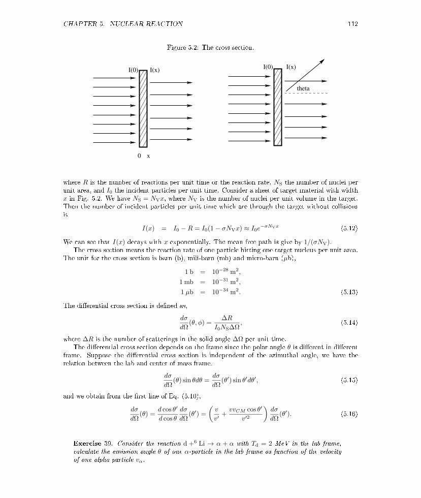
CHAPTER 5. NUCLEAR REACTION 112
Figure 5.2: The cross section.
I(x)
theta
0 x
I(0)I(0) I(x)
where R is the number of reactions per unit time or the reaction rate, NS the number of nuclei perunit area, and I0 the incident particles per unit time. Consider a sheet of target material with widthx in Fig. 5.2. We have NS = NVx, where NV is the number of nuclei per unit volume in the target.Then the number of incident particles per unit time which are through the target without collisionsis
I(x) = I0 −R = I0(1− σNVx) ≈ I0e−σNVx (5.12)
We can see that I(x) decays with x exponentially. The mean free path is give by 1/(σNV).The cross section means the reaction rate of one particle hitting one target nucleus per unit area.
The unit for the cross section is barn (b), mili-barn (mb) and micro-barn (µb),
1 b = 10−28 m2,
1 mb = 10−31 m2,
1 µb = 10−34 m2. (5.13)
The dierential cross section is dened as,
dσ
dΩ(θ, φ) =
∆R
I0NS∆Ω, (5.14)
where ∆R is the number of scatterings in the solid angle ∆Ω per unit time.The dierential cross section depends on the frame since the polar angle θ is dierent in dierent
frame. Suppose the dierential cross section is independent of the azimuthal angle, we have therelation between the lab and center of mass frame,
dσ
dΩ(θ) sin θdθ =
dσ
dΩ(θ′) sin θ′dθ′, (5.15)
and we obtain from the rst line of Eq. (5.10),
dσ
dΩ(θ) =
d cos θ′
d cos θ
dσ
dΩ(θ′) =
(v
v′+vvCM cos θ′
v′2
)dσ
dΩ(θ′). (5.16)
Exercise 39. Consider the reaction d +6 Li → α + α with Td = 2 MeV in the lab frame,calculate the emission angle θ of one α-particle in the lab frame as function of the velocityof one alpha particle vα.

CHAPTER 5. NUCLEAR REACTION 113
Exercise 40. Derive Eq. (5.16).
5.2 Partial wave analysis and optical potential
The elastic, inelastic and total cross section are
σel =π
k2
∞∑l=0
(2l + 1)|1− Sl|2
σin =π
k2
∞∑l=0
(2l + 1)(1− |Sl|2)
σtot =2π
k2
∞∑l=0
(2l + 1)(1− ReSl) (5.17)
where Sl = |Sl|e2iδl(k) and δl(k) is the phase shift. Having |1−Sl|2 = 1− 2ReSl + |Sl|2, we can verify
σtot = σel + σin (5.18)
In nuclear reaction, the elastic scattering can be further divided into potential and resonancescatterings
σel = σpot + σres (5.19)
So the total cross section can be decomosed in several dierent ways,
σtot = σel + σin
= σpot + σres + σin
= σpot + σa
= σpot + σCN + σD (5.20)
where σa = σres +σin = σCN +σD, with σCN,σD the formation cross sections of compound nuclei anddirect reaction respectively.
The idea of the optical potential is to treat a nucleus as a semi-opaque ball. When incident particlehits the nucleus part of it is reected or scattered, the other part of it is absorbed. It is convenientto introduce the optical potential,
Veff(r) =
−(V0 + iU), r ≤ R0, r > R
(5.21)
with the nuclear radius R. The wave function is in the form,
ψ = Aeikcx (5.22)
where
kc =√
2m(T + V0 + iU)
≈√
2m(T + V0) + iU
√m
T + V0
= k + ik′ (5.23)
where T is the kinetic energy of the incident particle. So the wave function have a damping part,
ψ = Aeikcx = Aeikxe−k′x (5.24)

CHAPTER 5. NUCLEAR REACTION 114
Figure 5.3: Optical potential [4].
The absorption rate is proportional to e−2k′x. The the typical attenuation length is given by
l =1
2k′=
1
2U
√T + V0
m(5.25)
We can estimate the mean free path when a neutron with energy T = 10 MeV hits a nucleus withpotential V0 = 40 MeV and U = 1 MeV. We obtain l ≈ 23 fm, which is much larger than nuclear size.We conclude that such a neutron can go through the nucleus almost without collisions.
More precisely the square well potential can be replaced by Woods-Saxon potential as
Veff(r) = − V0(V0 + iU)
1 + e(r−R)/a(5.26)
where a is the width of the nuclear surface. For nuclear reaction induced by neutron and proton, thespin-orbital term can be included into the potential.

CHAPTER 5. NUCLEAR REACTION 115
Figure 5.4: Types of scatterings [4].
5.3 Resonance and compound nuclear reaction
Compound nuclear reaction is one of low energy nuclear reaction and was rst proposed by N. Bohrin 1936. It can be written as
a + X→ C∗ → Y + b (5.27)
where C∗ denotes the compound nucleus. The cross section for the above reaction is
σab = σaΓb
Γ(5.28)
where σa is the formation cross section for the compound nucleus C∗, Γ is the total decay width ofthe compound nucleus C∗, and Γb is the decay width for the b-channel. When the incident particle(nucleus or nucleon) enters the nucleus X it strongly interacts with surrounding nucleons incide Xand quickly loses its energy to the surrounding nucleons to reach equilibrium and then form theexcited compound nucleus C∗. The excitation energy levels are well discretized for low excitations.So the cross section has a resonance feature. For higher excitations, the energy levels are continuousso the cross section varies slowly with energy, which is called continuum region. The transition fromresonance to continuum depends on the energy and nucleus atomic number. The compound nucleusin the excited state will decay by emitting a number of nucleons or a nucleus.
We can derive the resonance cross section. The total cross section is
σtot =4π
k
∞∑l=0
(2l + 1)Imfl(0)
=4π
k2
∞∑l=0
(2l + 1) sin2 δl(E) (5.29)
where is fl = (Sl − 1)/(2ik) with Sl = e2iδl(k). When δl(E) satisfy
δl(E) ∼ (n+ 1/2)π, or sin2 δl(E) ∼ 1 (5.30)
the partial wave cross section reaches maximum and the resonant states occur. We can expand near

CHAPTER 5. NUCLEAR REACTION 116
Figure 5.5: Test the compound nuclear reaction model. See An Experimental Verication of theTheory of Compound Nucleus, Phy. Rev. 80, 939(1950).

CHAPTER 5. NUCLEAR REACTION 117
the resonant energy E = E0 as
sin δl(E) ≈ sin δl(E0) +
[cos δl(E)
dδldE
]E0
(E − E0) ≈ 1
cos δl(E) ≈ cos δl(E0)−[sin δl(E)
dδldE
]E0
(E − E0)
= − dδldE
∣∣∣∣E0
(E − E0) = − 2
Γ(E − E0) (5.31)
where we have dened
Γ = 2/dδldE
∣∣∣∣E0
(5.32)
So the partial wave amplitude The we have
fl =1
kexp[iδl(k)] sin δl(k)
=1
k
sin δl(k)
cos δl(k)− i sin δl(k)
≈ 1
k
1
− 2Γ (E − E0)− i =
1
k
−Γ/2
(E − E0) + iΓ/2
Imfl =1
k
Γ2/4
(E − E0)2 + Γ2/4(5.33)
If at E ∼ E0, the partial wave l is dominant, the cross section is then
σtotl =
π
k2(2l + 1)
Γ2
(E − E0)2 + Γ2/4(5.34)
We can extend the above formula into the compound nuclear reaction a + X→ C∗ and choose thelowest partial wave. The cross section is then
σa =π
k2
ΓaΓ
(E − E0)2 + Γ2/4(5.35)
where Γ is the total width and Γa is the partial width for the a-channel. So the cross section forreaction (5.27) is then
σab =π
k2
ΓaΓb
(E − E0)2 + Γ2/4(5.36)
For incident nuclei with spins and resonance with non-zero spin, we should also include a spin countingfactor g = (2IC + 1)/[(2Ia + 1)(2IX + 1)], where IC, Ia and IX are spins of the resonance, incidentparticle and target nucleus respectively.
To test the compound nuclear reaction model, Ghoshal measured p +6329 Cu and α+60
28 Ni to form6430Zn∗,
p +6329 Cu → 64
30Zn∗ →
6330Zn + n6230Zn + 2n6229Cu + p + n
α+6028 Ni → 64
30Zn∗ →
6330Zn + n6230Zn + 2n6229Cu + p + n
(5.37)

CHAPTER 5. NUCLEAR REACTION 118
The data show that
σp,n : σp,2n : σp,pn = σα,n : σα,2n : σα,pn = Γn : Γ2n : Γpn (5.38)
which predicted by the model.The angular distribution of nucleon emitted by compound nuclei is almost isotropic without
preferable direction, i.e. the compound nuclei lose the memory of the incident particle's direction.The emission of outgoing particles is like evaporation. This is not surprising since the energy of theincident particle is distributed among all nucleons in the nucleus. The more energy is pumped intothe nuclei, more particles are likely to evaporate.
Exercise 41. The Breit-Wigner formula for the single-level compound cross section in thenuclear reaction a+X → C∗ is
σab = gπ
k2
ΓaΓb
(E − E0)2 + Γ2/4
where g = (2IC +1)/[(2Ia +1)(2IX +1)], IC, Ia and IX are spins of the compound nucleus orresonance, incident particle and target nucleus respectively. Consider the compound nucleus(resonance) reaction n +235
92 U→ C∗ with IU = 7/2 and In = 1/2. At neutron energies below0.5 eV, the cross section is dominated by one resonance with IC = 3 at a kinetic energy of0.29 eV with a width of 0.135 eV. There are three channels, which allow the compound stateto decay by neutron emission, photon emission, or ssison. At resonance the contributionsto the neutron cross sections are (a) elastic and resonant scattering ( 1 barn); (b) radiativecapture (70 barns); (c) ssion (200 barns). The questions: (1) Calculate the partial widthsfor the three channels. (2) How many ssions per second will there be in a sheet of U-235of thickness 1mg/cm−2, traversed by normally by a neutron beam of 105 per second with akinetic energy of 0.29 eV?
5.4 Direct reaction
Stripping reaction is one kind of direct reaction, where the projectile nucleus loses some of its con-stituents to the target nucleus and the rest of it pass through as nal nucleus. Stripping reaction fordeuteron is a normal type and can be denoted as
AZX(D,p)A+1
Z YAZX(D,n)A+1
Z+1Y (5.39)
For example, we have3H(D,n)4He, 32S(D,p)33S, 27Al(D,p)28Al (5.40)
Nuclear ssion and fusion are also direct reactions.Knock-out reaction is another type of direct reaction, where the projectile nucleus knocks out
some constituents of the target and stays in the target or emits with less energy. For example,
p +157 N→ p +14
7 N + n (5.41)
The transfer reaction is a reaction type where a number of protons or neutrons of the projectileleave in the target or the projectile grab a number of protons or neutrons from the target nuclear.For example,
178 O +12
6 C → 168 O +13
6 C21H +20
10 Ne → 11H +21
10 Ne21H +14
7 N → 32He +13
6 C (5.42)

CHAPTER 5. NUCLEAR REACTION 119
Figure 5.6: Examples for stripping and kock-out reactions.
dZ,A
initial state final state
p
Z,A
p
p
n
initial state final state
Z,A−1
Z,A+1
Another example is the reaction in which the neutron was rst discovered by Chadwick in 1932,
42He +9
4 Be→ n +126 C (5.43)
It is also used for generating neutrons in the lab. The helium-4 particles come from radioactiveamericium, and the beryllium is just a piece of metal.
Neutron absorption is a reaction where a neutron is absorbed by a nucleus, for example,
n +2713 Al → 28
13Al→ 2812Mg + p + νe
n +23592 U → 236
92 U→ 23290 Th + α (5.44)
Note that aluminum-28 and uranium-236 are very unstable and decay very quickly through β and αdecay respectively.
Another important nuclear reaction is the heavy ion collisions, where two heavy nuclei collide eachother.
5.5 Nuclear ssion
Nuclear ssion is phenomenon where a nucleus split to two fragments of approximately equal mass.The nuclear ssion was discovered in 1939 by Hahn and Strassmann when they found the uraniumatom, when bombarded by neutrons, can produce barium, a much lighter element than uranium.
There are two types of nuclear ssions: the spontaneous ssion and induced ssion. The spon-taneous ssion happens without any outside perturbations. The induced ssion needs an absorptionof additional particles, e.g. a slow neutron, to excite the nucleus and fragment into smaller pieces.Induced ssion takes place in nuclear reactors.
5.5.1 Spontaneous ssion
In order for the spontaneous ssion to take place, ssile nuclei must overcome the Coulomb barrier,see Fig. 5.7(a). We take U-238 for example. We assume it split into two equal daughter nuclei

CHAPTER 5. NUCLEAR REACTION 120
Figure 5.7: (a) Droplet model for ssion. Fission barrier is about 6 MeV. (b) The ssion barrier as afunction of mass number.
whose surface touch. Then the distance between two daughter nuclei can be approximated as R =2× 1.2× (238/2)1/3 ≈ 14.9 fm. We can estimate the Coulomb potential as follows,
V =(Z/2)2e2
R=
462 × 197
14.9× 137≈ 204 MeV. (5.45)
This is roughly the energy released in ssion. The ssion barrier or the activation energy as a functionof mass number can be shown in Fig. 5.7(b).
Now we rst discuss about the spontaneous ssion in detail. We take a very simple example, amother nucleus splits into two daughters,
AZX→ A1
Z1Y1 + A2
Z2Y2 (5.46)
where A = A1 +A2 and Z = Z1 + Z2. The Q-value is
Q = aS(A2/3 −A2/31 −A2/3
2 ) + aC(Z2A−1/3 − Z21A−1/31 − Z2
2A−1/32 )
= aS[A2/3 −A2/31 − (A−A1)2/3]
+aC[Z2A−1/3 − Z21A−1/31 − (Z − Z1)2(A−A1)−1/3] (5.47)
We resuire that Q is stable with respect to varying A1 and Z1, i.e.
∂Q
∂A1=
2
3aS[−A−1/3
1 + (A−A1)−1/3]
+1
3aC[Z2
1A−4/31 − (Z − Z1)2(A−A1)−4/3] = 0
∂Q
∂Z1= 2aC[−Z1A
−1/31 + (Z − Z1)(A−A1)−1/3] = 0 (5.48)
which gives A = 2A1 and Z = 2Z1. The stability of the nucleus with respect to the ssion is thatthe Q-value is less than zero, with A = 2A1 and Z = 2Z1, the threshold condition is then
Q(A1 = A/2, Z1 = Z/2) = aS(1− 21/3)A2/3 + aC(1− 2−2/3)Z2
A1/3= 0 (5.49)

CHAPTER 5. NUCLEAR REACTION 121
whose solution isZ2
A=
aS(21/3 − 1)
aC(1− 2−2/3)≈ 0.7
aS
aC≈ 18 (5.50)
where we have used aS ≈ 17.8 MeV and aC ≈ 0.71 MeV. Note that Q is an increasing function of A,then we conclude that nuclei with A . 70 are stable with respect to spontaneous ssion.
Like alpha decay, the spontaneous ssion is also a quantum tunneling eect. For the spontaneousssion to take place the Q-value must be equal to the Coulomb barrier at the distance of scission fortwo daughter nuclei or at 2R1,
aS(1− 21/3)A2/3 + aC(1− 2−2/3)Z2
A1/3=Z2
1e2
2R1(5.51)
where R1 ≈ r0A1/31 ≈ r02−1/3A1/3 and Z1 ≈ Z/2. Then the solution is
Z2
A=
aS(1− 21/3)
e2/(r028/3)− aC(1− 2−2/3)
≈ 0.26aS
0.37aC − 0.16e2r−10
≈ 2.25aS
aC≈ 56 (5.52)
where we have used r0 = 1.25 fm, e2 = 1/137, e2/r0 ≈ 1.62aC with aC = 0.71 MeV and aS = 17.8MeV. The stability condition for spontaneous ssion is Z2/A . 56. So we nd a heavy nucleus withA ≈ 226 and Z ≈ 113 cannot have spontaneous ssion. Of course this is a very rough estimation.
Bohr explained the spontaneous ssion using the nuclear droplet model, see Fig. 5.7. The de-formation is assumed to be the reason for the ssion. Nuclear density or volume is almost constantunder small deformations. A sphere has the smallest ratio of surface area to volume. If the sphere isdeformed to ellipsoid at constant density its surface area and surface energy will increase. Since thedeformation makes charges separate, the Coulomb energy will decrease. The surface tension tendsto make the deformed nucleus recover to sphere, while the Coulomb potential tends to make thenucleus be even more deformed. That the nucleus will be stable or unstable for a small deformationdepends on whether the increase of surface energy outperforms the decrease of Coulomb energy. Thedeformation can be described by a long ellipsoid with the half lengths of the long axis and short axisare r1 = R(1 + a) and r2 = R/
√1 + a respectively. The Coulomb and surface energies are
EC(a) =1
2
∫dV dV ′
1
|r− r′|ρ(r)ρ(r′) =3
5
Q2
R
(1− a2
5
)= aCZ
2A−1/3
(1− a2
5
)ES(a) = 4πR2σ
(1 +
2a2
5
)= aSA
2/3
(1 +
2a2
5
)(5.53)
where we have used
V =4π
3r1r
22 =
4π
3R3
S = 2π
[r22 +
r1r2 sin−1 e
e
](5.54)
where e =√
1− (r2/r1)2. The change in the binding energy of the deformed nucleus is from theCoulomb and surface energy,
∆E = EC(a) + ES(a)− EC(0)− ES(0)
= −aCZ2A−1/3 a
2
5+ aSA
2/3 2a2
5= aSA
2/3 2a2
5(1− x) (5.55)
where x = aC2aS
Z2
A . Here we have used 35Q2
R = aCZ2
A1/3 and 4πR2σ = aSA2/3. When x < 1, the binding
gets positive correction, so the nucleus is stable against the spontaneous ssion, when x > 1, thebinding gets negative correction, the nucleus is unstable against the ssion.

CHAPTER 5. NUCLEAR REACTION 122
Figure 5.8: The potential energy of a nucleus as a function of deformation parameter Z2/A. (a)Z2/A 0.7 aSaC ; (b) Z
2/A & 0.7 aSaC ; (c) Z2/A . 2.6 aSaC ; (d) Z
2/A > 2.6 aSaC .
(a) (b)
(c) (d)

CHAPTER 5. NUCLEAR REACTION 123
Exercise 42. Suppose a mother nucleus splits into two eqaul daughters,
AZX→ A1
Z1Y + A2
Z2V
where A1 = A2 = A/2 and Z1 = Z2 = Z/2. The coecients in the nuclear bindingenergy are: aV ≈ 15.75 MeV (volume energy term), aS ≈ 17.8 MeV (surface energy term),aC ≈ 0.71 MeV (Coulomb energy term), asym ≈ 23.3 MeV (symmetric energy term), aP ≈ 12MeV (pairing energy term). (1) Express the Q-value of the above ssion reaction. (2)In order for the ssion to take place, Q value must be no less than the Coulomb barrierZ2
1e2/(2R1), try to estimate the critical value of Z2/A at which ssion can take place. Here
R1 = r0A1/31 and r0 = 1.2 fm. (3) If we further assume Z = A/2, what would A be for
ssible nuclei?
5.5.2 Induced ssion
The uranium nucleus 23592 U can have ssion when absorbing a slow neutron which makes 236
92 U in anexcited state with excitation energy obtained by,
Sn(236U) = m(235U) +mn −m(236U)
= ∆(235U) + ∆mn −∆(236U)
= 40.91 + 8.07− 42.44 ≈ 6.54 MeV (5.56)
where ∆ denotes the nuclear mass excess relative to atomic mass unit (931.5 MeV) times the atomicnumber. We see that Sn(236U) ≈ 6.54 MeV is larger than its ssion barrier 5.9 MeV.
But 238U cannot undergo ssion with a slow neutron. The dierence is that 236U is an even-even nucleus whose binding energy is larger with full pairings of neutrons while 239U is an even-oddnucleus whose binding energy is smaller. The uranium nucleus 239U tends to decay to its groundstate through emitting a γ photon. Since 236U is tightly bound, so it tends to split into nearly equallymassive fragments. By capturing a slow neutron, the excitation energy of 239U is
Sn(239U) = m(238U) +mn −m(239U)
= ∆(238U) + ∆mn −∆(239U)
= 47.3 + 8.07− 50.6 ≈ 4.8 MeV (5.57)
which is not enough to overcome the ssion barrier 6.2 MeV. Here are reactions of 238U when capturinga slow neutron,
23892 U + n → 239
92 U∗ → 23992 U + γ
23992 U → 239
93 Np + e- + ν23993 Np → 239
94 Pu + e- + ν (5.58)
Here 23994 Pu is ssionable element since it is an even-odd nucleus. The abundances of 235U and 238U
are 0.7% and 99.3% on the earth. 23992 U and 239
94 Pu do not exist on the earth.The ssion cross sections for 235U/238U or 235U(n, f)/238U(n, f) are shown in Figs. 5.9 and 5.11.
In the thermal region, the cross section has 1/v behavior. In the energy range 1-100 eV there aremany resonances produced. For U-235, the cross section for ssion induced by thermal neutrons is3 orders of magnitude larger than by fast neutrons. For U-238, ssion cannot occur in the thermalregion.
As we have shown before that the ssionable nuclei are heavy nuclei, the heavier the nuclei are themore neutrons they have because the number of neutron increases with the mass number. Thereforethe fragments have more neutrons and away from beta-stable line. These neutrons are called prompt
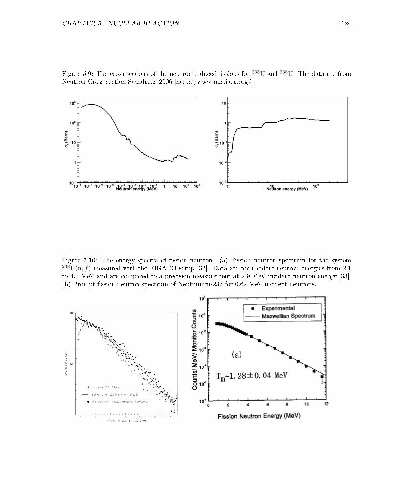
CHAPTER 5. NUCLEAR REACTION 124
Figure 5.9: The cross sections of the neutron induced ssions for 235U and 238U. The data are fromNeutron Cross-section Standards 2006 [http://www-nds.iaea.org/].
Neutron energy (MeV)−8
10 −710−6
10−5
10 −410−3
10 −210 −110 1 10210
310
(B
arn
)f
σ
−110
1
10
210
310
Neutron energy (MeV)1 10
210
(B
arn
)f
σ
−310
−210
−110
1
10
Figure 5.10: The energy spectra of ssion neutron. (a) Fission neutron spectrum for the system238U(n, f) measured with the FIGARO setup [32]. Data are for incident neutron energies from 2.1to 4.0 MeV and are compared to a precision measurement at 2.9 MeV incident neutron energy [33].(b) Prompt ssion neutron spectrum of Neptunium-237 for 0.62 MeV incident neutrons.
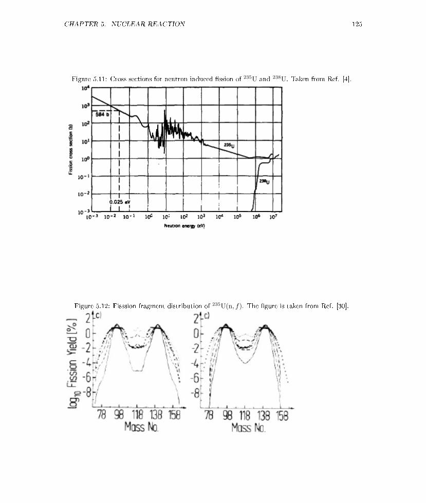
CHAPTER 5. NUCLEAR REACTION 125
Figure 5.11: Cross sections for neutron induced ssion of 235U and 238U. Taken from Ref. [4].
Figure 5.12: Fisssion fragment distribution of 235U(n, f). The gure is taken from Ref. [30].

CHAPTER 5. NUCLEAR REACTION 126
Figure 5.13: Delayed neutron emission from Rb-93. Taken from Ref. [4].
neutrons because they emitted in less than 10−15s. Their distribution is isotropic. The ssionfragments normally undergo beta decay and followed by more neutron emission. These neutrons arecalled delayed neutron. The delay time is of order of a few seconds. For example, following the6-seconds beta decay of 93
37Rb→ 9338Sr∗ + e− + νe, the excited state 93
38Sr∗ has a larger enough energythan neutron separation energy, so it can decay by neutron emission in competition with Gammaemission, 93
38Sr∗ → 9238Sr+n. The delay neutrons are normally used to controll chain reactions in ssion
reactors. See Fig. 5.13 for the scheme plot of the above beta decay and delayed neutron emission.The energy spectra of the prompt neutrons follows Maxwell distribution
f(E) ∼√E exp(−E/Tm) (5.59)
where TM is called Maxwell temperature of about one or two MeV, see Fig. 5.10. The example forthe neutron energy spectra are those in the spontaneous ssion of 252
98 Cf and in the induced ssion of23592 U with thermal neutrons, where Tm are
Tm[25298 Cf] = 1.453± 0.017 MeV
Tm[23592 U + nth] = 1.319± 0.019 MeV (5.60)
The average energy of neutrons is 3Tm/2. The number of neutrons follows the Gauss distribution
P (λ) =1√2πσ
exp
[− (λ− λ)
2σ2
](5.61)
where λ is the average number of neutrons including prompt and delayed neutrons, which is about2 to 4 for most nuclei. For thermal induced ssion of 233U, 235U and 238U, the average numbers ofprompt neutrons are 2.48, 2.42, 2.86 respectively.

CHAPTER 5. NUCLEAR REACTION 127
The probability for a ssionable nucleus to split to two equal fragments is very small. Normallythere is a distribution of ssion fragments as a function of mass number, for example the fragmentsof 235U(n, f) follow the distribution as shown in Fig. 5.12. The most probable fragments for inducedssion reaction 235U(n, f) are around A1 = 95 and A2 = 140. This is a typical example for inducedssion,
n +23592 U → 93
37Rb +14155 Cs + 2n
5.5.3 Self-sustaining nuclear ssions and ssion reactor
A nucleus of 235U absorb a slow neutron and undergoes ssion and release on average 193 MeV ofenergy. For example, the ssion reaction
n + 23592 U→ 92
36Kr + 14256 Ba + 2n (5.62)
has the Q-value
Q = m(23592 U)−m(92
36Kr)−m(14256 Ba)−mn
= [235.04− (91.93 + 141.92)− 1.0] u
= 0.19 u ≈ 177 MeV (5.63)
Most of them is converted to thermal energy. On average 2.5 prompt neutrons and 0.018 delayedneutrons are produced in each ssion process. If at least one neutron is captured by the 235U nucleithe nuclear ssion is then self-sustaining with constant output of energy.
In natural uranium material on the earth the self-sustaining ssion can not take place since 99.28%of ingredients are 238U. The ssions of 238U rely on higher energy neutrons of above 1 MeV but theneutrons quickly lose their energies via inelastic scatterings. In the 1 MeV region the cross sectionof 238U(n, γ)239U is 1/10 of 235U(n, f) but the aboundance of 238U is 138 times that of 235U. So innatural uranium most neutrons produced in ssions of 235U are absorbed by 238U which stop furtherssions. There are two methods to solve this problem: either to enrich 235U or to change the energyspectra of neutrons to enhance the cross section of 235U(n, f) over 238U(n, γ)239U. The latter methodcan be realized by thermalization of neutrons. Note that the ssion cross section of 235U follows a1/v =
√mn/2E law, the smaller v the larger the cross section.
Through elastic scattering of light nuclei, fast neutrons of about 1 MeV can lose their energiesvery quickly. Now we can estimate how much energy a neutron would lose in each collision. Supposein the lab frame a neutron with velocity vn collides with a nucleus of mass M which is still, thescattered neutron moves in the direction θ in the center-of-mass frame. The center-of-mass frame hasa velocity vCM = mnvn/(mn +M) in the lab frame. So in the lab frame the energy is
EL =1
2mn[((vn − vCM) cos θ + vCM)2 + (vn − vCM)2 sin2 θ]
=1
2mn[(vn − vCM)2 + v2
CM + 2(vn − vCM)vCM cos θ] (5.64)
The average energy over angle θ is then
EL =12mn
∫d cos θ[(vn − vCM)2 + v2
CM + 2(vn − vCM)vCM cos θ]∫d cos θ
=1
2mn[(vn − vCM)2 + v2
CM] =1
2mn
m2n +M2
(mn +M)2v2
n (5.65)
So the fraction of EL in the incident energy Ein becomes
EL
Ein=
M2n +M2
(Mn +M)2(5.66)

CHAPTER 5. NUCLEAR REACTION 128
If M → ∞, the lab frame coincides with the center-of-mass frame, so the neutron would not loseenergy by elastic scatterings. If we use carbon as a moderator with mass M ≈ 12Mn, the fractionbecomes EL/Ein = 145/169 ≈ 0.86, i.e. the neutron loses 14% of its energy per scattering. For aneutron of 1 MeV it will undergo 6 ln(10)/ ln(1/0.86) ≈ 91 collisions to reach 1 eV. One would thinkthat hydrogen would be best choice for the moderator but the cross section of p(n, γ)d is very largeso that it is not suitable. But hydrogen in the form of heavy water D2O or some compound canbe used as the moderator in the reactor with enriched uranium. Graphite is the material used asa moderator in natural uranium because 12C is a light nucleus and all nucleons are in pairs so thenucleus is tightly bound.
5.5.4 Time constant of a ssion reactor
The neutron number distribution in a reactor is a function of the time, position and energy of theneutron. For an ideal case, we consider a homogeneous number density n for neutrons. Due to thecapture processes for these neutrons, the number of neutrons will decrease as follows dn/dt = −n/τwhose solution is n = n0e
−t/τ . Here τ is the time constant and given by
1
τ=∑i
σivNi (5.67)
where σi and Ni are the cross section and particle number density for the i-th process and nucleusi respectively. For a neutron with energy 1/40 eV, the cross sections are 238U(n, γ)239U: 2.73 barns,235U(n, f): 577 barns, 235U(n, γ)236U: 101 barns.
If we include the production of neutrons, the rate equation becomes
dn
dt= (k − 1)
n
τ(5.68)
where k is the neutron reproduction or multiplication factor and dened as the ratio of the numberof neutrons in one generation to the that in proceeding generations. It reects the net change in thethermal neutron number between two generations. The solution to the above equation is then
n = n0e(k−1)t/τ (5.69)
Only if k ≥ 1, will the number density of neutrons increase, and then the ssion is self-sustaining.If k > 1, we call it super-critical. If k = 1, we call it critical. If k < 1, we call it sub-critical. Theneutron reproduction factor k is dened by
k = ηfεp (5.70)
This is known as four-factor formula. Here f is the thermal fuel utilization factor for neutrons whichgives the fraction of neutrons available to U-235 and U-238. It is dened by
f =NUσa(U)∑
iNiσa(i) +NUσa(U)(5.71)
where σa(i) is the absorption (including ssion) cross section for nuclide i. The factor η is dened asthe mean number of ssion neutrons produced per thermal neutron in the last generation, which isgiven by
η(U) = λσf(U)
σf(U) + σa(U)(5.72)
where σa(U) is the absorption cross section by uranium. For example, for natural uranium and 1/40eV neutrons, we have σf(
235U) = 577 b, σa(235U) = 101 b, σf(238U) = 0 b and σa(238U) = 2.73 b,
then we can obtain
σf(U) = 0.0072σf(235U) + 0.9928σf(
238U) = 4.15 b
σa(U) = 0.0072σa(235U) + 0.9928σa(238U) = 3.43 b

CHAPTER 5. NUCLEAR REACTION 129
With λ = 2.5, we get the factor η(U) = 1.37. One way to increase η(U) is to enrich uranium.For natural uranium, a fast neutron can induce 238U to undergo ssion which will also produce
neutrons, so ε is the factor for induced ssion by fast neutrons (fast-ssion factor) and dened by
ε =Nfast +Nthermal
Nthermal(5.73)
where Nfast and Nthermal are neutron numbers from induced ssion by fast and thermal neutronsrespectively. In natural uranium before cooled down to thermal energy resonant absorption takesplace for some neutrons.
The escape rate from such resonance absorption is denoted by resonance escape probability p.Here ε and p depend on the geometric shape of the reactor.
5.6 Accelerator-Driven System
5.6.1 Spallation neutron source
Neutrons have many properties that make them an ideal tool for certain types of research. Neutronsare neutral and are highly penetrating. So they can be used as clean and non-destructive probe tomaterials. Neutrons are very sensitive to hydrogen, they can locate hydrogen atoms and then todetermine the structure of molecules or materials. Neutrons are also sensitive to light atoms amongheavy ones. This properties have been used to locate light oxygen atoms in yttrium-barium-copperoxide (YBCO), a high-Tc superconducting ceramic, whose positions in the ceramic are crucial tothe superconducting properties. Neutrons have spin and magnetic moment. Such a property makesneutron act like a compass needle to detect the magnetic structure of materials and help developenew magnetic materials. The energies of thermal neutrons almost match those of atoms in motion,or in other words, the neutron wavelength is close to the atomic spacing, so neutrons can be usedto track molecular vibrations, movements of atoms during catalytic reactions, and crystal structuresand atomic spacings, etc..
Neutron sources have been built to meet the needs in many elds. The Spallation NeutronSource (SNS) is an accelerator-based neutron source in Oak Ridge, Tennessee , USA, at the site ofOak Ridge National Laboratory by the U.S. Department of Energy (DOE). Spallation is a process inwhich fragments of material (spall) are ejected from a body due to impact or stress. In nuclear physicsis the process in which a heavy nucleus emits a large number of nucleons as a result of being hit by ahigh-energy particle. The SNS uses high-energy protons to bombard a target made of heavy particlesto produce many neutrons. For each collision 20 to 30 neutrons are ejected. The neutron energiesare about 30 MeV for proton beam with 1 GeV. For more about SNS, see http://www.sns.gov/.
These neutrons can be used to bombard nuclear fuel to make sustainable nuclear ssion. This iscalled the Accelerator-Driven sysytem (ADS). The neutrons produced by spallation act as a trigger toignite the ssion which will continue by additional neutrons produced in the course of ssion. Thereis an advantage for the ADS system is that the ssion will stop immediately once the proton beam isswitched o, therefore an ADS is safer than conventional reactor. For more information about ADS,see, e.g., http://www.world-nuclear.org/.
5.6.2 Thorium as ssion fuel
Thorium reservation on the earth is 3 to 5 times that of uranium. Thorium can be used as ssionfuel by capturing a neutron,
n +23290 Th→ 233
90 Th (22 min)→ 23391 Pa (27 days)→ 233
92 U (159200 years) (5.74)
which is analogous to
n +23892 U→ 239
92 U (23.5 min)→ 23993 Np (2.4 days)→ 239
94 Pu (24110 years) (5.75)

CHAPTER 5. NUCLEAR REACTION 130
Figure 5.14: Fission cross section of Uranium-233.
The process of converting fertile isotopes to ssile ones is called breeding. Uranium-233 needs enoughneutrons to undergo sustainable ssion. Carlo Rubbia rst proposed to use ADS to produce enoughneutrons to ignite sustainable ssion of Thorium-232.
5.6.3 Nuclear waste incinerator
Used nuclear fuel in conventional reactors normally contain a lot of long-lived heavy isotopes, par-ticularly actinides. Among nuclides heavier than Th-232, those with odd atomic number can mostprobably absorb a neutron to undergo ssion, while those with even atomic number will rst undergobeta-decay and then ssion. ADS can be used to transmute these long-lived isoptopes into short-livedones. ADS can also be used to destroy long-lived ssion product such as Tc-99 and I-129.
5.7 Nuclear fusion
As can be seen in the behavior of the binding energy per nucleon versus the mass number, two lightnuclei lower than iron in mass merge into a middle sized nucleus can release energy. This process iscalled fusion. There are many types of nuclear fusion, among which are thermonuclear fusion, inertialconnement fusion, beam-beam and beam-target fusion etc.. Nuclear fusion have been known topower the stars. H. Bethe found the main cycle of nuclear fusion in stars in 1930s. The hydrogenbomb was successful in 1952 as part of the Manhattan Project. Civilian use of fusion power is notsuccessful until now because for the fusion to take place two light nuclei have to overcome the Coulombbarrier which needs extremely high temperature environment.
The Coulomb barrier is shown in Fig. 5.15 and is given by
EB =Z1Z2e
2
R(5.76)
where R = r0(A1/31 +A
1/32 ), and Z1 and Z2 are proton numbers for incident nuclei. The turning point

CHAPTER 5. NUCLEAR REACTION 131
is
Rtp =Z1Z2e
2
E(5.77)
where E = 12mrv
2 with the reduced mass mr = m1m2/(m1 + m2) of two incident nuclei and theirrelative velocity v. The barrier transparency factor T is given by,
T ≈ e−G ≈ e−√EG/E = e−2πZ1Z2e
2/v (5.78)
where EG = 2mr(Z1Z2e2π)2 is called the Gamow energy. The above is valid for EG E. The
tunneling factor G can be evaluated as,
G = 2√
2mr
∫ Rtp
R
dr√V (r)− E
= 4√
2mrERtp
∫ 1
y0
dy√
1− y2
≈√EG
E, for R Rtp (5.79)
where V (r) = Z1Z2e2/r, y =
√r/Rtp and y0 =
√R/Rtp. We see that the Coulomb barrier is
extremely sensitive to Z1Z2. The less Z1Z2, the most probably the fussion reaction can take place.The barrier is the lowest for hydrogen isotopes, EB ∼ e2/R ∼ 100/137 ∼ 0.7 MeV. This is still muchlarger than typical kinetic energy of a few KeV.
The fusion cross section is normally parameterized as
σ ≈ σgeomTF (5.80)
where σgeom is the geometrical cross section and F is the reaction characteristic factor and dependson the nature of the reaction. The geometrical cross section σgeom is given by the wavelength of theinduced mass,
σgeom ∼ λ2 ∼ 1
(mrv)2∼ 1
mrE(5.81)
So the fussion cross section can be nally written as
σ(E) =S(E)
Ee−√EG/E (5.82)
where S(E) is called astrophysical S-factor, a weakly energy dependent function for non-resonantreactions.
The reaction rate per unit volume for two collision particles is given by
R12 =n1n2
1 + δ12〈σv〉 (5.83)
where σ is the cross section for the reaction,v is the relative velocity, n1 and n2 are number densities.If two colliding particles are identical δ12 = 1, otherwise δ12 = 0. In thermal environment, the velocityobeys Boltzmann-Maxwell distribution, then 〈σv〉 is evaluated as
〈σv〉 = N−1
∫dv v2σv exp(−βmrv
2/2)
= 2N−1m−2r
∫ ∞0
dES(E) exp[−(√
EG/E + βE)]
(5.84)

CHAPTER 5. NUCLEAR REACTION 132
where β = (kBT )−1 and
N =
∫ ∞0
dv v2e−mrv2/(2kBT ) =
√2
m3/2r
∫dE√Ee−βE
=√
2
(kBT
mr
)3/2 ∫ ∞0
dx√xe−x =
√2
(kBT
mr
)3/21
2Γ
(1
2
)=
√π
2
(kBT
mr
)3/2
(5.85)
is the normalization constant. Inserting the above into Eq. (5.83), we obtain the reaction rate. Herewe have used the cross section formula in Eq. (5.82). The energy integral in Eq. (5.84) is dominated
by the minimum value of the function f(E) =√
EG
E + βE in the exponent at E0,
df(E)
dE= −1
2
√EGE
−3/20 + β = 0
E0 = E1/3G
(kBT
2
)2/3
(5.86)
So we can expand f(E) =√
EG
E + βE at E = E0 and keep the quadratic term,
f(E) ≈ f(E0) +1
2
d2f(E)
dE2
∣∣∣∣E=E0
(E − E0)2
= f(E0) +3
8E
1/2G E
−5/20 (E − E0)2 (5.87)
So Eq. (5.84) becomes
〈σv〉 ≈ 2N−1m−2r S(E0) exp
[−(√
EG/E0 + βE0
)]∫ ∞
0
dE exp
[−3
8E
1/2G E
−5/20 (E − E0)2
]≈ 24/3
√3π
(Z1Z2e2π)1/3(kBT )−2/3m−1/3
r S(E0) exp
[− 3
22/3
(EGkBT
)1/3]
(5.88)
The Sun is a perfect prototype of self-sustaining thermonuclear fusion reactor. The basic fusionprocess in the sun is the hydrogen burning process into helium. Hydrogen is the most abundantmaterial in the universe, almost 90% of elements in the universe are hydrogens. The temperature inthe center of the Sun is about 1.6× 10⁷ K (about 1.38 KeV with 1 eV = 1.1604× 10⁴ K). Most fusionreactions occur within 25% of the Sun's radius (R = 6.95× 10⁵ km). Most of the sun energy comesfrom the proton-proton chain reaction. The reaction rate in the center is about 9.2 × 1037 timesper second. In each reaction four protons are converted into alpha particles or Helium-4. So about3.7× 1038 proton out of 1057 protons are converted to Helium-4 per second. Each fusion releases theenergy of about 25.7 MeV (or 27.8 MeV if including electron-positron annihilation), see below. Thusthe energy power is about (3− 4)× 1026 W (1 W = 1 J · s−1 = 107 erg · s−1).
The proton-proton chain reaction of type-I (pp-I chain) is,
p + p → D + e+ + νe + 0.42 MeV
e+ + e− → 2γ + 1.02 MeV
p + D → 32He + γ + 5.49 MeV
32He + 3
2He → 42He + 2p + γ + 12.86 MeV (5.89)

CHAPTER 5. NUCLEAR REACTION 133
Figure 5.15: Coulomb barrier for fusion.
alpha−potential
energy−barrier
energy−alpha
−v−zero
radius−R radius−rturningpoint
Note that in denition of the Q-value we did not count the electron in the nal state. If we do nottake the second reaction for electron-positron annihilation into account, the net reaction is
4p→ 42He + 2e+ + 2νe + 3γ + 24.68 MeV (5.90)
when including electron-positron annihilation, the net reaction becomes
4p + 2e− → 42He + 2νe + 7γ + 26.70 MeV (5.91)
The pp-I branch is dominant at temperatures of 10 to 14 megakelvins (MK = 106 K). Below 10 MK,the 4
2He yield is suppressed. Since in the rst reaction a proton must be converted to a neutron in theweak interaction. The rate is controlled by the rst reaction since the time scale for weak interactionis much longer than the strong interaction. The cross section is of order 10−33 b and 10−23 b at KeVand MeV respectively. The proton number density of the core of the Sun is about 7.5 × 1025 cm−3,and the temperature is about 16 MK. Given these parameters, we can estimate the rate of the rstreaction, which is actually the rate of the pp-chain.
The pp-II chain is more important for temperatures of 14 to 23 MK. The pp-II chain reaction is
32He + 4
2He → 74Be + γ + 1.59 MeV
74Be + e− → 7
3Li∗(73Li) + νe + 0.861(0.383) MeV
73Li + p → 24He + 17.35 MeV (5.92)
whose net reaction is32He + p + e− → 4He + νe + 19.8/19.3 MeV (5.93)
90% of the neutrinos produced in the reaction 7Be(e−, νe)7Li∗ carry an energy of 0.861 MeV (Lithium-
7 in the excited state), while the remaining 10% carry 0.383 MeV (Lithium-7 in the ground state).If the temperature is above 23 MK, there is pp-III chain reaction as follows,
32He + 4
2He → 74Be + γ + 1.59 MeV
74Be + p → 8
5B + γ + 0.197 MeV85B → 8
4Be + e+ + νe + γ + 17.5 MeV84Be → 24
2He + 0.092 MeV (5.94)

CHAPTER 5. NUCLEAR REACTION 134
Figure 5.16: Parameters for some fusions. The Q-value is only from nuclear mass dierence. The tableis from S. Atzeni and J. Meyer-Ter-Vehn, The Physics of Inertial Fusion: Beam Plasma Interaction,Hydrodynamics, Hot Dense Matter, Oxford University Press, 2009. The data is from C. Angulo etal., Nucl. Phys. A656 (1999)3-187. [http://pntpm.ulb.ac.be/Nacre/nacre_d.htm]

CHAPTER 5. NUCLEAR REACTION 135
Figure 5.17: The pp chain reaction in the sun. Fromhttp://en.wikipedia.org/wiki/File:FusionintheSun.svg.

CHAPTER 5. NUCLEAR REACTION 136
whose net reaction is32He + p→ 4He + e+ + νe + 3γ + 19.3 MeV (5.95)
The pp III chain is not a major source of energy for the Sun (only 0.11%), but was very importantin the solar neutrino problem because it generates very high energy neutrinos (up to 14.06 MeV).
The CNO cycle is more important for heavier stars and higher temperatures (called CNO-I),
126 C + p → 13
7 N + γ + 1.94 MeV137 N → 13
6 C + e+ + νe + 1.71 MeV136 C + p → 14
7 N + γ + 7.55 MeV147 N + p → 15
8 O + γ + 7.30 MeV158 O → 15
7 N + e+ + νe + 2.24 MeV157 N + p → 12
6 C + 42He + 4.96 MeV (5.96)
The net reaction is4p→ 4
2He + 2e+ + 2νe + 3γ + 27.8 MeV (5.97)
Note that the Carbon, Nitrogen and Oxygen nuclei do not really participate the net reaction butplay as catalyst. The net reaction is still Eq. (5.91). There are also another chain reactions calledCNO-II invloving 16
8 O and 179 O.
The pp-chain and CNO cycle are not feasible on the earth because there is anything that canconne the matter at such high temperatures in such a long time. The fusion reactions which can beused on the earth are those with large cross sections at moderate temperatures. For example, hereare a few such reactions,
31H + 2
1H → 42He + n + 17.58 MeV (DT)
31H + 3
1H → 42He + 2n + 11.33 MeV (TT)
21H + 2
1H → 32He + n + 3.27 MeV (DD)
→ 31H + p + 4.04 MeV
→ 42He + γ + 23.85 MeV
21H + 3
2He → 42He + p + 18.4 MeV
Because of large energy release, the DT reaction is chosen for controlled fussion reaction in reactors.

CHAPTER 5. NUCLEAR REACTION 137
Figure 5.18: The cross sections for DD and DT fusion reactions. Also shown is the fusion reaction ofHe-3 and deuteron. Taken from [4].

CHAPTER 5. NUCLEAR REACTION 138
Figure 5.19: The cross sections for DD and DT fussion reactions averaged over Boltzmann-Maxwelldisribution. Also shown is the fusion reaction of He-3 and deuteron. Taken from [4].
Exercise 43. The Sun is a perfect prototype of self-sustaining thermonuclear fusion reactor.The basic fusion process in the sun is the hydrogen burning process into helium. The proton-proton chain reaction of type-I (pp-I chain) is dominant one,
p + p → D + e+ + νe
p + D → 32He + γ
32He + 3
2He → 42He + 2p + γ
Given the atomic masses (not nuclear mass, given by mass excess relative to atomic massunit) of nuclides MD = 12.628 MeV, MHe3 = 14.931 MeV, MHe4 = 2.425 MeV. Theproton and neutron masses (mass excess) are mp = 0.007276 u, mn = 0.008665 u with1 u = 931.494 MeV/c2. The electron mass is me = 0.511 MeV. (1) Calculate the Q-value ofeach reaction. The Q-value is dened as the mass surplus of initial state nuclei relative tonal state nuclei. (2) Write the net reaction and the Q-value. (3) Among the three reactions,which one is dominant to control the total reaction rate? Why? (4) The fusion cross sectionof the rst reaction p + p→ D + e+ + νe can be written as
σ(E) =S(E)
Ee−√EG/E
where E = mrv2/2 is the kinetic energy with reduced mass of two incident nuclei mr =
m1m2/(m1 + m2), and EG = 2mr(Z1Z2e2π)2, S(E) = S(0) + (dS(0)/dE)E with S(0) =
3.8×10⁻²² KeV·barn and dS(0)/dE = 4.2×10⁻²⁴ barn. We note that the fusion takes placewithin 25% of the Sun's radius (R = 6.95× 10⁵ km) and the proton mass density is about100 g/cm3. We can approximate that the kinetic energy E is given 3T/2 with T = 1.6× 10⁷
K. For reference we list following constants here: 1 MeV= 1.16×10¹⁰ K, Avogadro's constantNA = 6.022 × 10²³/mol, barn=10−24 cm2. Try to calculate the rate of the fusion reactionper unit volume.

CHAPTER 5. NUCLEAR REACTION 139
[Solution: E = 3T/2 = 2.07 KeV, S(E)/E ≈ 1.9 × 10⁻²² barn, EG ≈ 940 × 103 × π2/1372 ≈494 KeV,
√EG/E ≈ 15.4, e−
√EG/E = 1.95 × 10⁻⁷. σ = 3.6 × 10⁻²⁹ barn= 3.6 × 10−53 cm2.
v =√
2E/mr =√
4.14× 10⁻³/940 = 2.09 × 10⁻³ → 6.3 × 107 cm/s. σv = 2.3 × 10−45 cm3/s.nH = 100×6.022×1023 = 6×1025/cm3. R/V = n2
Hσv/2 = 5.76×10⁶ s−1cm−3. R = 1.92×10⁻¹⁹/s,τ = 1/R = 5.2× 10¹⁸ s= 1.65× 10¹¹ y.]
Chapter 6
Nuclear force and nucleon-nucleon
interaction
6.1 Properties of nucleons
The proton and neutron are nucleons, the building blocks of nuclei. The properties of nucleons aresummarized in Table 6.1. The main dierence between the proton and the neutron is that the mass ofthe neutron is 1.29 MeV larger than that of the proton and that the proton is stable but the neutronis not. The dominant decay mode for the neutron is n→ p+ e− + νe.
6.2 General properties of nuclear force
The human knowledge about nuclear force started from 1934, shortly after neutron was discoveredin 1932 by J. Chadwick. Then H. Yukawa proposed that nuclear force was mediated by meson whichwas discovered in 1947. From modern perspective nuclear force can understood as a residual forceof strong interaction whose the elementary particles are quarks and gluons. Mesons are actuallycomposite particles made of quarks and gluons. Nuclear force is like a Van der Waals force amongatoms which is a short range force much weaker than electromagnetic force. The Van der Waalsforce originated from separation of charges (electric polarization) in atoms which are electric neutral.Similarly quarks and gluons are bound together into a nucleon which is a color singlet object (colorneutral). When quarks and gluons with colors uctuate inside the nucleon they produce a shortrange force felt by a neighboring nucleon. Therefore the nuclear force is a residual force of quarksand gluons.
1. Saturation and short distance. The forces which bind the nucleons together in nuclei are very
Table 6.1: Properties of nucleons.
proton neutronquark content uud udd
I(JP ) 12
(12
)+ − 12
(12
)+mass 938.27203±0.00008 MeV 939.56536±0.00008 MeV
Magnetic moment 2.792847351±0.000000028 µN −1.9130427±0.0000005 µNCharge radius 0.875 ± 0.007 fm − 0.1161±0.0022 fmMean life > 2.1×1029 years 885.7±0.8 s
140

CHAPTER 6. NUCLEAR FORCE AND NUCLEON-NUCLEON INTERACTION 141
Figure 6.1: Nuclear force mediated by meson. From http://en.wikipedia.org/wiki/Nuclear_force.
Figure 6.2: The nuclear force.
100
200
1 2
middleshort long
r (fm)
V (MeV)

CHAPTER 6. NUCLEAR FORCE AND NUCLEON-NUCLEON INTERACTION 142
Table 6.2: The states of NN system denoted by the symbol 2S+1L. B, H, M and W mean Bartlett,Heisenberg, Majorana and Wigner force.
NN state L S I σ1 · σ2 τ1 · τ2 B H M Wpp,np,nn 1S 0 0 1 -3 1 1 1 -1 -1
np 3S 0 1 0 1 -3 -1 -1 -1 -1np 1P 1 0 0 -3 -3 1 -1 1 -1
pp,np,nn 3P 1 1 1 1 1 -1 1 1 -1
strong because they can at least overcome the Coulomb repulsion among protons. The nuclear forceshave one property which we call the saturation: a nucleon can only interact with nucleons surroundingit in a nucleus because it is an attractive force at short distances. This is why the binding energy isproportional to the number of nucleons in a nucleus or the atomic number A. We can easily understandit. Suppose the nuclear forces in the nucleus would be attractive between all pairs of nucleons, thenthe total potential exerted on one nucleon by other A− 1 nucleons is proportional to (A− 1). Thereare A nucleons, so the total potential energy is proportional to A2, which is not the real case. Theremust be some other eects to keep the nucleons apart when the inter-nucleon distance is larger thana threshold value. It turns out to be that the nuclear force is attractive in the intermediate shortrange r ∈ [1, 2] fm and repulsive at very short distance r ∈ [0, 1] fm, where r is the distance betweentwo nucleons. In some sense the nuclear force is like Van der Waals force of molecules, which arisesfrom inhomogeneous distributions of electric charges though the molecule does not carry net chargesor is electric neutral. The nuclear force is illustrated in Fig. 6.2.
2. Exchange property. Nuclear force is mediated by mesons (pions and others) like the covalentbonding in molecules. The force is attractive or repulsive depending on if the pair of nucleons is ina symmetric or an anti-symmetric state in their separation. This counts in part for the saturationof the forces. If we regard the proton and nucleon as an isospin doublet, we can extend the Pauliprinciple by including the isospin. For a NN system, the total wavefunction must be anti-symmetricwith respect to exchange of two nucleons, which requires
(−1)L+S+I = −1 (6.1)
Assume ψ(r1, σ1, τ1; r2, σ2, τ2) is the wavefunction of the NN system, where σi and τi (i = 1, 2)label the spin and isospin states. We introduce three exchange operators Pr, Pσ and Pτ whichexchange the spatial positions, spins and isospins of two nucleons,
Prψ(r1, σ1, τ1; r2, σ2, τ2) = ψ(r2, σ1, τ1; r1, σ2, τ2)
Pσψ(r1, σ1, τ1; r2, σ2, τ2) = ψ(r1, σ2, τ1; r2, σ1, τ2)
Pτψ(r1, σ1, τ1; r2, σ2, τ2) = ψ(r1, σ1, τ2; r2, σ2, τ1) (6.2)
These operators satisfyP 2r = P 2
σ = P 2τ = 1 (6.3)
So the eigenvalues of the above operators must be ±1. Considering the properties under the exchangeof positions, spins and isospins for a NN state with the angular momentum, spin and isospin quantumnumber L, S and I,
Pr = (−1)L
Pσ = (−1)S+1
Pτ = (−1)I+1 (6.4)
According to Eq. (6.1), we have
PrPσPτ = −1 (6.5)

CHAPTER 6. NUCLEAR FORCE AND NUCLEON-NUCLEON INTERACTION 143
These operators can be expressed in terms of Pauli matrices for spins and isospins σ1,2 and τ1,2,
Pσ = (1 + σ1 · σ2)/2 = S(S + 1)− 1
Pτ = (1 + τ1 · τ2)/2 = I(I + 1)− 1
Pr = −(1 + σ1 · σ2)(1 + τ1 · τ2)/4 (6.6)
One can check S(S + 1)− 1 = (−1)S+1 for S = 0, 1.In nucleon-nucleon interaction, the nuclear force can be modeled by nuclear potential in Schroedinger
equation. The most widely used nucleon-nucleon potentials are the Paris potential, the Argonne po-tential, the Bonn potential and the Nijmegen potentials. The parameters of these potentials are xedby tting experimental data, such as the deuteron binding energy, nucleon-nucleon elastic scatteringcross sections, etc.. A recent development is to systematically derive the nucleon-nucleon potentialfrom chiral eective eld theory. Nuclear potential can be classied into four kinds, they are attractiveor repulsive depends on the quantum state of the nucleon-nucleon system. In the following, vW(r),vM(r), vH(r) and vB(r) are all positive functions.
Spin exchange potential (Bartlett force),
VB = −1
2(1 + σ1 · σ2)vB(r) (6.7)
The spin exchange potential is attractive for the spin triplet state S = 1 and repulsive for thesinglet S = 0.
Isospin exchange potential (Heisenberg force),
VH =1
2(1 + τ1 · τ2)vH(r) (6.8)
The isospin exchange potential is attractive for the isospin singlet state I = 0 and repulsive forthe triplet I = 1.
Space exchange potential (Majorana force),
VM =1
4(1 + σ1 · σ2)(1 + τ1 · τ2)vM(r) (6.9)
Non-exchange potential (Wigner force),
VW = −vW(r) (6.10)
We see that the non-exchange potential is always attractive.
In the above we note that vW(r), vM(r), vH(r) and vB(r) are all positive functions. As shown inTable 6.2, the above four forces are all attractive for the state 3S.
3. Charge independence or isospin invariance. The nuclear force between two nucleons is equalirrelevant of if they are proton-proton, neutron-neutron or proton-neutron,
Vpp ≈ Vnn ≈ Vpn (6.11)
This property was veried in the NN scattering experiments and in the presence of isospin multipletsin nuclear structure. A good example is the mirror nuclei 3H and 3He (see Fig. 6.3). It is found thatthe dierence in binding energies of 3H and 3He only comes from the Coulomb energy of proton-protonin 3He.
4. Momentum dependence. The nuclear force nontrivially depends on the relative momentum dueto the fact that it is mediated by meson exchange. The most important force that is momentumdependent is the LS coupling,
(L · S)V (r) (6.12)

CHAPTER 6. NUCLEAR FORCE AND NUCLEON-NUCLEON INTERACTION 144
Figure 6.3: Mirror nuclei: 3H and 3He.
p
n n
p
p n
which is essential to explain the shell structure of in nuclei.5. Spin dependent. Apart from the spin exchange force listed in Eq. (6.7), there is also tensor
force formed by three vectors σ1, σ2 and r = r/|r|,
S12 = 3(r · σ1)(r · σ2)− (σ1 · σ2) = (3rirj − δij)σ1iσ2j
= 6(S · r)2 − 2S2 (6.13)
The tensor force violates the angular momentum conservation.In summary, the nuclear force has the following general form,
V = Vc(r) + Vσ(r)(σ1 · σ2) + Vτ (r)(τ1 · τ2) + Vστ (r)(σ1 · σ2)(τ1 · τ2)
+VI(r)S12 + VIτ (r)S12(τ1 · τ2) (6.14)
One sees that the potential conserves the total isospin since it is commutable with
I2 =1
4(τ1 + τ2)2 =
1
2(3 + τ1 · τ2) (6.15)
The potential does not depend on I3, i.e. it does not discriminate protons and neutrons.NN potentials have the following properties,
A scalar, because it is an energy;
Only depends on the relative distance between two nucleons r and σ ·r- locality and momentumconservation;
Invariant under the spatial reection - parity invariance;
Invariant under rotation - angular momentum conservation;
Invariant under the time reection;
Invariant under the exchange of proton and neutron;
Not dependent on velocity - static;
Exercise 44. What is general Pauli exclusive principle? From this principle, ll the emptyspace of the following table,
NN state L S I σ1 · σ2 τ1 · τ2 B H M Wpp,np,nn 1S 1 1 -1 -1
np 3S -1 -1 -1 -1np 1P 1 -1 1 -1
pp,np,nn 3P -1 1 1 -1

CHAPTER 6. NUCLEAR FORCE AND NUCLEON-NUCLEON INTERACTION 145
Table 6.3: Static properties of the deuteron nucleus (JP = 1+).
observables databinding energy BD (MeV) 2.224magnetic moment µD/µN 0.857
electric quadrupole QD (fm2) 0.286
average square root radius⟨√
r2⟩(fm) 1.964
ratio of D to S states η = AD/AS 0.026
Exercise 45. What is the saturation property of nuclear force?
Exercise 46. Assume ψ(r1, σ1, τ1; r2, σ2, τ2) is the wavefunction of the nucleon-nucleonsystem, where σi and τi (i = 1, 2) label the spin and isospin states. We introduce operatorsPσ and Pτ which exchange the spins and isospins of two nucleons,
Pσψ(r1, σ1, τ1; r2, σ2, τ2) = ψ(r1, σ2, τ1; r2, σ1, τ2)
Pτψ(r1, σ1, τ1; r2, σ2, τ2) = ψ(r1, σ1, τ2; r2, σ2, τ1)
Considering that the nucleon-nucleon state can be in spin and isospin singlet and triplet,write down the formula for Pσ and Pτ using σi and τi.
6.3 Deuteron nucleus
The Deuteron nucleus is the second most simple nuclei and made of one proton and one neutron.Following the Pauli principle 6.1, the total wave function must be anti-symmetric with the exchangeof two nucleons. The Deuteron nucleus is an isospin singlet and has spin-parity JP = 1+. Theinteraction inside the deuteron is purely nuclear force without Coulomb contribution. Since S = 1gives a stronger nuclear attraction, the deuterium ground state is in the S = 1, L = 0 state. As weknow from the positive parity and total angular momentum 1 of the deuteron, it must be in the stateswith relative orbital angular momentum L = 0, 2, · · · , where two lowest states are 2S+1LJ =3 S1,
3D1.
6.3.1 S-state
For the 3S1 state, the relative motion of neutron and proton can be described by Schrödinger equationwith a square well potential, [
− 1
mN∇2 + V (r)− E
]ψ(r) = 0 (6.16)
Here the reduced mass is mN/2. The square well potential is dened by,
V (r) =
−V0, (r ≤ a)0, (r > a)
(6.17)
Since the deuteron nucleus is in the S-state, the wave function only depends on the radius r,
ψ(r) = u(r)/r (6.18)

CHAPTER 6. NUCLEAR FORCE AND NUCLEON-NUCLEON INTERACTION 146
Then the Schrödinger equation becomes[− 1
mN
1
r2
d
drr2 d
dr+ V (r)− E
]u(r)
r= 0 (6.19)
Using
1
r2
d
drr2 d
dr=
d2
dr2+
2
r
d
drd2
dr2
u(r)
r=
u′′(r)
r− 2
r3(ru′ − u)
2
r
d
dr
u(r)
r=
2
r3(ru′ − u) (6.20)
the the Schrödinger equation can be simplied as
− 1
mNu′′(r) + [V (r)− E]u(r) = 0 (6.21)
and further as
u′′(r) +mN[E + V0]u = 0, (r ≤ a)
u′′(r) +mNEu = 0, (r > a) (6.22)
where the energy is chosen to be the binding energy E = BD = −2.224 MeV. Using the boundarycondition, u(0) = u(∞) = 0, we get the solution
u(r) =
A sin(
√mN(E + V0)r), (r ≤ a)
B exp(−√mN|E|r), (r > a)
(6.23)
At r = a, u(r) and u′(r) must be continuous. So we get
A sin(√mN(E + V0)a) = B exp(−
√mN|E|a)
A√mN(E + V0) cos(
√mN(E + V0)a) = −B
√mN|E| exp(−
√mN|E|a) (6.24)
and then
1√mN(E + V0)
tan(√mN(E + V0)a) = − 1√
mN|E|(6.25)
which gives the relation between V0 and a. We can choose a = 2 fm. Dene ka =√mN|E|a ≈√
938× 2.224× 2/197 ≈ 0.465 and k0a ≡√mNV0a, with k < k0, the above equation is rewritten as
tan(√
(k0a)2 − (ka)2) = −√
(k0a)2 − (ka)2
ka(6.26)
In order for the above equation to have solutions, k0a must be within [(2n + 1/2)π, (2n + 1)π] sothat two functions y = tan
√x2
0 − x2 and y = −x−1√x2
0 − x2 (x0 ≡ k0a, x ≡ ka) have intersections.For ka ≈ 0.465, we can nd the smallest value k0a ≈ 1.87 which is about 1.19 times π/2 and within[π/2, π]. In this case, the potential depth is V0 = 36.5 MeV.
The electric dipole moment of the deuteron is zero. Its magnetic moment is
µJ = µL + µS = gLµNL + gSµNS = gJµNJ (6.27)
where J, L and S are the total, orbital and spin momenta. gi=J,L,S are their g-factors, and wehave gL = (gp
L + gnL)/2 = gp
L/2 = 1/2 and gS = (gpS + gn
S)/2. The g-factor of deuteron for oribital

CHAPTER 6. NUCLEAR FORCE AND NUCLEON-NUCLEON INTERACTION 147
angular momentum can be easily understood by the fact that only proton contributes with half oftotal orbital angular momentum: µL = gp
LµNLp = gpLµNL/2. The g-factor of deuteron for spin can
also be derived:
µS = gSµNS =1
2µN(gp
Sσ1 + gnSσ2)
gSS · S =1
4(gpSσ1 · S + gn
Sσ2 · S)
=3
4(gpS + gn
S) +1
4(gpS + gn
S)σ1 · σ2 (6.28)
where we have used S = 12 (σ1 + σ2). We see that for S = 1, gS = (gp
S + gnS)/2.
We multiply J to both sides of Eq. (6.27) and obtain
gJJ · J =1
2gpL(L · J) +
1
2(gpS + gn
S)(S · J)
gJJ = gpLJ(J + 1) + L(L+ 1)− S(S + 1)
4(J + 1)
+(gpS + gn
S)J(J + 1) + S(S + 1)− L(L+ 1)
4(J + 1)(6.29)
Then the magnetic moments of the deuteron states 3S1 (S = 1, J = 1 and L = 0) and 3D1 (S = 1,J = 1 and L = 2) are
µJ(3S1) = gJJ =1
2(gpS + gn
S) = 0.879
µJ(3D1) = gJJ =3
4gpL −
1
4(gpS + gn
S) = 0.31 (6.30)
We can see we can reproduce the magnetic moment of deuteron nucleus in such a simple model.
6.3.2 S and D states
Data show that the deuteron has non-zero quadrupole moment, indicating that one should take non-central potential into account. The most simple non-central potential is the tensor one, then the totalpotential of the deuteron can be written as
V (r) = Vc(r) + S12VT(r) (6.31)
where the tensor operator S12 is given in Eq. (6.13). As we have mentioned in the last subsectionthat the lowest ground states of the deuteron are states 3S1 and 3D1. Let us denote φS and φD asthe spin and angular part of the S- and D-state wavefunction,
φ1MS = χ1MY00(θ, φ)
φ1MD =
∑M1,M2
c(M ;M1,M2)Y2M1(θ, φ)χ1M2 (6.32)
where the Clebsch-Gordon coecients c(m;m1,m2) can be taken from [19] and are listed below,
c(1; 2,−1) =√
3/5, c(1; 1, 0) = −√
3/10, c(1; 0, 1) =√
1/10
c(0; 1,−1) =√
3/10, c(0; 0, 0) = −√
2/5, c(0;−1, 1) =√
3/10
c(−1; 0,−1) =√
1/10, c(−1;−1, 0) = −√
3/10, c(−1;−2, 1) =√
3/5 (6.33)

CHAPTER 6. NUCLEAR FORCE AND NUCLEON-NUCLEON INTERACTION 148
The spin wave functions are
χ1,1 = ↑↑
χ1,0 =1√2
(↑↓ + ↓↑)
χ1,−1 = ↓↓ (6.34)
and angular momentum ones are
Y2,2(θ, φ) =1
4
√15
2πsin2 θe2iφ =
1
4
√15
2π
1
3
(T 11 − T 22 + i2T 12
)Y2,1(θ, φ) = −
√15
8πsin θ cos θeiφ = −
√15
8π
1
3
(T 13 + iT 23
)Y2,0(θ, φ) =
√5
4π
(3
2cos2 θ − 1
2
)=
1
2
√5
4πT 33
Y2,−m(θ, φ) = (−1)mY ∗2,m(θ, φ) (6.35)
where the rand-2 tensor is dened by T ij = 3rirj − δij . With Eq. (6.13), one can prove
S12φ1MS =
√8φ1M
D
S12φ1MD =
√8φ1M
S − 2φ1MD (6.36)
Now we can introduce the D wavefunction into the ground state of the deuteron,
ψ(r) =√PSψS(r) +
√PDψD(r)
=u(r)
rφ1MS +
w(r)
rφ1MD (6.37)
Then PS and PD are given by
PS =
∫ ∞0
∣∣∣∣u(r)
r
∣∣∣∣2 r2dr =
∫ ∞0
u2(r)dr
PD =
∫ ∞0
∣∣∣∣w(r)
r
∣∣∣∣2 r2dr =
∫ ∞0
w2(r)dr
PS + PD =
∫ ∞0
[u2(r) + w2(r)]dr = 1 (6.38)
The Schrödinger equation becomes[− 1
mN∇2 + Vc(r) + S12VT(r)− E
]ψ(r) = 0 (6.39)

CHAPTER 6. NUCLEAR FORCE AND NUCLEON-NUCLEON INTERACTION 149
We can simplify it by[− 1
mN∇2 + Vc(r) + S12VT(r)− E
](u(r)
rφ1MS +
w(r)
rφ1MD
)=
[− 1
mN∇2 + Vc(r)− E
](u(r)
rφ1MS +
w(r)
rφ1MD
)+S12VT(r)
(u(r)
rφ1MS +
w(r)
rφ1MD
)=
[− 1
mN∇2 + Vc(r)− E
](u(r)
rφ1MS +
w(r)
rφ1MD
)+VT(r)
(u(r)
r
√8φ1M
D +w(r)
r
√8φ1M
S − w(r)
r2φ1M
D
)=
[− 1
mN∇2 + Vc(r)− E
]u(r)
rφ1MS +
w(r)
r
√8VT(r)φ1M
S
+
[− 1
mN∇2 + Vc(r)− E
]w(r)
rφ1MD + VT(r)
(√8u(r)
r− 2
w(r)
r
)φ1MD = 0 (6.40)
The we get [− 1
mN∇2 + Vc(r)− E
]u(r) + w(r)
√8VT(r) = 0[
− 1
mN∇2 + Vc(r)− 2VT(r)− E
]w(r) +
√8VT(r)u(r) = 0 (6.41)
The boundary conditions areu(r), w(r) = 0, r = 0,∞
The coupled equations can be solved numerically. The solutions have to be adjusted to t the data.These equations can be decoupled outside the range of nuclear force, the asymptotic behaviors are
u(r) = ASe−kr
w(r) = AD
[1 +
3
kr+
3
(kr)2
]e−kr (6.42)
with k =√mN|E|. The ratio of D to S state is
η = AD/AS ≈ 0.025 (6.43)
The electric quadrupole moment is
QD =⟨ψ|Q|ψ
⟩= PS
⟨ψS |Q|ψS
⟩+ PD
⟨ψD|Q|ψD
⟩+ 2√PSPD
⟨ψS |Q|ψD
⟩(6.44)
where the quadrupole operator is dened as
Q =1
4(3z2 − r2) =
√π
5r2Y20(θ) (6.45)
Note that the rst term in Eq. (2.39) does not contribute following the Wigner-Eckart theorem, i.e.there is no [1] in [5]⊗ [1] = [5]. Then we can derive
QD =
√2
10
∫ ∞0
drr2u(r)w(r)− 1
20
∫ ∞0
drr2w2(r) (6.46)

CHAPTER 6. NUCLEAR FORCE AND NUCLEON-NUCLEON INTERACTION 150
Exercise 47. The spin-parity of deuteron is JP = 1+. What are two lowest states fordeuteron? Express the states using the optical spectrum symbol 2S+1LJ with S, P,D,G, F, · · ·for L = 1, 2, 3, 4, 5, · · · .
Exercise 48. Prove Eq. (6.36).
Exercise 49. Prove Eq. (6.46).

CHAPTER 6. NUCLEAR FORCE AND NUCLEON-NUCLEON INTERACTION 151
Figure 6.4: pp cross sections
6.4 Low energy nucleon-nucleon scatterings
When considering nucleon-nucleon scatterings, we have spin-orbit and spin-spin interactions in ad-dition to the central potential. Neither spins nor orbital angular momenta are conserved in thescatterings. Only the total angular momentum, its third compponent and the parity are conserved.For a general two-to-two scattering a + b→ c + d , the selection rules for the interaction are
(1) PaPb(−1)L = PcPd(−1)L′
(2) ma +mb +mL = mc +md +mL′
(3) J = J ′ (6.47)
where Pi are intrinsic parities for particles i = a,b, c,d; mi are the third components of the spins;mL and mL′ are the third components of the relative angular momenta of initial and nal states; Jand J ′ are the total angular momenta of initial and nal states.
Nucleon-nucleon scatterings include np, pp and nn scatterings. One can measure the cross sections,dierential cross sections or angular distributions with or without polarizations. For low energyscatterings ka 1, s-wave is dominant. We can estimate the incident energy for which ka < 1 holds,ka ≈ √mnEa ≈
√mnEL/2a where EL is the energy in the lab frame. When EL ∼ 10 MeV and
a ∼ 2 fm, ka ∼ 0.7, so for EL < 10 MeV, we can safely consider only the s-wave. In this case thetotal cross section is
σtot ∼ 4π1
k2(P1 sin2 δ1 + P3 sin2 δ3) ≈ π(a2
s1 + 3a2s3) (6.48)
where δi and asi for i = 1, 3 are phase shifts and scattering lengths for the spin singlet and triplet.The total cross section is obtained by summing over all the nal states and taking average over theinitial states for which P1,3 = 1/4, 3/4 are degeneracy weights from spin counting. Since the totalangular momentum is conserved, there is no mixing of the singlet and triplet in the amplitude. FromEq. (??) and (A.62), we have
k coth δ1 = − 1
as1+
1
2reff,1k
2
k coth δ3 = − 1
as3+
1
2reff,3k
2 (6.49)
CHAPTER 6. NUCLEAR FORCE AND NUCLEON-NUCLEON INTERACTION 152
where reff,1,3 are eective force distances for the singlet and triplet. For neutron-proton scatterings,their values are given by
as1 ≈ 23.7 fm
reff,1 ≈ 2.5 fm
as3 ≈ −5.4 fm
reff,3 ≈ 1.7 fm (6.50)
Note that the triplet/singlet channel is attractive/repulsive since as3/as1 is negative/positive. Fromthe scattering length we can determine the depth of the potential provided the potential width a isknown following Eq. (A.63). If we set a = 3 fm, we have the potential depths for singlet and tripletchannels are 311 and 96 MeV respectively, corresponding to k0a = 1.51π, 0.46π. The total crosssection is then about 20.4 barns (10−24 cm2), where those for the singlet and the triplet are 71 and3.7 barns. From these value we can determine the potential depth and width from Eqs. (A.65,A.63).At low energy the phase shift as function of wave number are independent of potential shape becausethe wave length is much larger than the force distance. The scattering length for the triplet is negativemeans the phase shift is positive and the force is attractive.
6.5 Nucleon-Nucleon scatterings in moderate energy
To gain knowledge about the deep structure of the nuclear force, one has to use high energy scatterings.When the nucleon incident energy in the lab frame EL > 400 GeV, the internal mesonic degree offreedoms can be excited and the relativistic eects enter the play. New particles can be produced bytransforming part of the kinetic energy into the masses.
Suppose the incident protons are moving along the z-axis in proton-neutron scatterings. Thedierential cross section dσ/dΩ of neutron-proton scatterings in moderate energies has a feature thatthere are peaks at θ = 0, π and the peak at θ = π is higher than that at θ = 0. There is a valleyat θ = π/2. The large peak at θ = π is understood as the signal for the exchange character of thenuclear force. The protons can exchange a pion with the neutrons and turn to neutrons which emitat small angles, while the protons transformed from the incident neutron absorbing the pions moveout along the negative z-axis.
In proton-proton scatterings the dierential cross section shows an isotropic feature with respectto polar angles except θ < π/8. This is a result of coherence eect among a variety of partial waves.
6.6 Meson exchange model for NN potentials
Yukawa rst proposed in 1934 that in analogy to the scalar potential of the electromagnetic eld thereis also a potential between the proton and the neutron. The potential has an additional exponentialfactor besides the Coulomb potential,
V (r) = ge−λr
r
where g is the coupling constant and λ characterizes the distance of the nuclear force. He arguedthat λ is actually the mass of one kind of particle which mediate the nuclear force which was latercalled the pion.
Fig. 6.5 shows the central force, one can see that the repulsive part of the nucleon-nucleonpotential in short distance is from the vector meson exchange ω and ρ. For intermediate distance thepotential is dominated by the σ meson exchange. The long distance part is from the pion exchange.The tensor force is provided by the pion and the ρ meson, while the spin-orbital force is from the σand ω mesons.
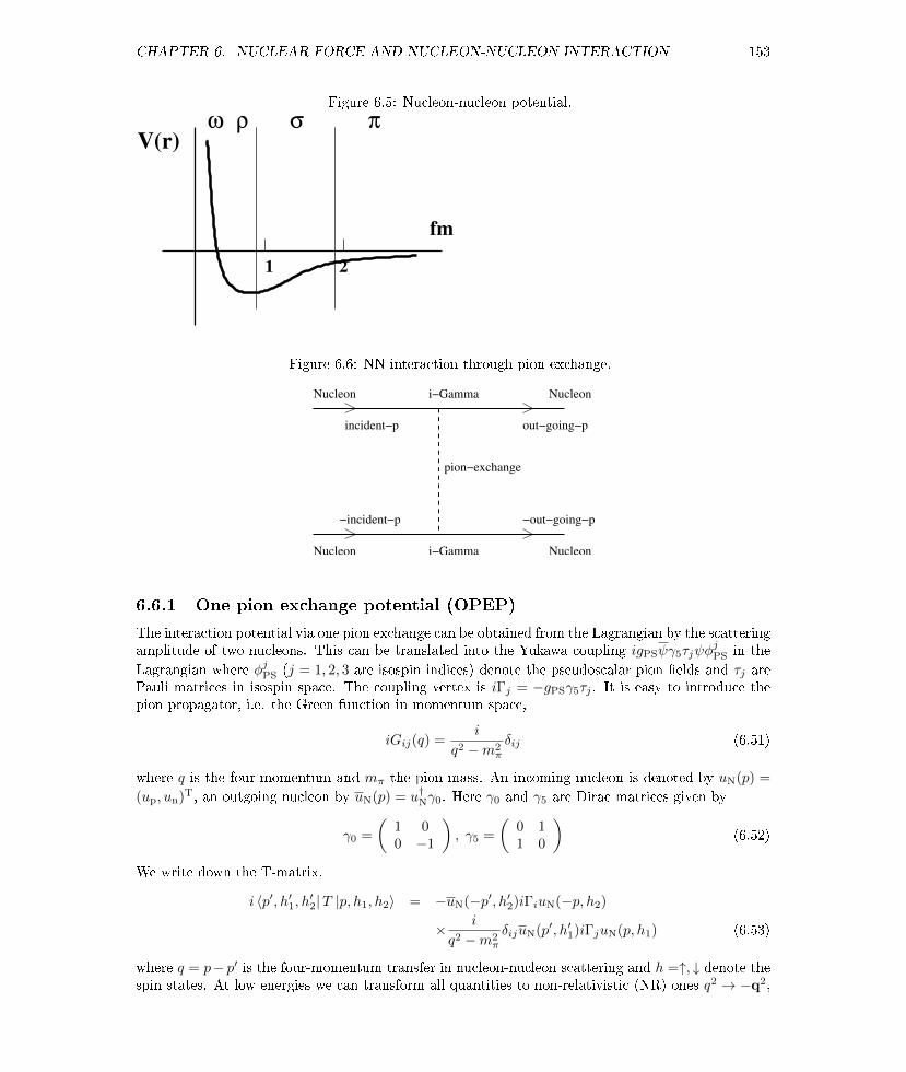
CHAPTER 6. NUCLEAR FORCE AND NUCLEON-NUCLEON INTERACTION 153
Figure 6.5: Nucleon-nucleon potential.
ρω σ π
1 2
fm
V(r)
Figure 6.6: NN interaction through pion exchange.
incident−p out−going−p
Nucleon
Nucleon
Nucleon
Nucleon
i−Gamma
i−Gamma
pion−exchange
−incident−p −out−going−p
6.6.1 One pion exchange potential (OPEP)
The interaction potential via one pion exchange can be obtained from the Lagrangian by the scatteringamplitude of two nucleons. This can be translated into the Yukawa coupling igPSψγ5τjψφ
jPS in the
Lagrangian where φjPS (j = 1, 2, 3 are isospin indices) denote the pseudoscalar pion elds and τj arePauli matrices in isospin space. The coupling vertex is iΓj = −gPSγ5τj . It is easy to introduce thepion propagator, i.e. the Green function in momentum space,
iGij(q) =i
q2 −m2π
δij (6.51)
where q is the four-momentum and mπ the pion mass. An incoming nucleon is denoted by uN(p) =
(up, un)T, an outgoing nucleon by uN(p) = u†Nγ0. Here γ0 and γ5 are Dirac matrices given by
γ0 =
(1 00 −1
), γ5 =
(0 11 0
)(6.52)
We write down the T-matrix,
i 〈p′, h′1, h′2|T |p, h1, h2〉 = −uN(−p′, h′2)iΓiuN(−p, h2)
× i
q2 −m2π
δijuN(p′, h′1)iΓjuN(p, h1) (6.53)
where q = p− p′ is the four-momentum transfer in nucleon-nucleon scattering and h =↑, ↓ denote thespin states. At low energies we can transform all quantities to non-relativistic (NR) ones q2 → −q2,

CHAPTER 6. NUCLEAR FORCE AND NUCLEON-NUCLEON INTERACTION 154
EN → mN and
uN(p, h) =
(χ(h)
σ·pE+mN
χ(h)
)→(
χ(h)σ·p2mN
χ(h)
)(6.54)
where χ = (χp, χn)T with χp,n = |↑〉 , |↓〉 are Pauli spinors for spin states. We obtain
uN(p′, h′1)γ5τjuN(p, h1) = 〈χ(1′)| ( 1, σ·p′2mN
)
(1 00 −1
)(0 11 0
)τj
(1
σ·p2mN
)|χ(1)〉
=1
2mN〈χ(1′)|σ · (p− p′)τj |χ(1)〉
uN(−p′, h′2)γ5τiuN(−p, h2) = − 1
2mN〈χ(2′)|σ · (p− p′)τi |χ(2)〉 (6.55)
Then the T-matrix element in the non-relativistic limit can be simplied by
〈p′, h′1, h′2|T |p, h1, h2〉NR
= − g2PS
4m2N(q2 +m2)
〈χ(1′)| (σ · q)τi |χ(1)〉 〈χ(2′)| (σ · q)τi |χ(2)〉 (6.56)
which give rise to the eective potential in the Born approximation,
Vπ(q) = − g2PS
4m2N
1
q2 +m2π
(τ1 · τ2)(σ1 · q)(σ2 · q) (6.57)
The potential in coordinate space can be obtained by Fourier transformation,
Vπ(r) =
∫d3q
(2π)3eiq·rV (q)
=g2
PS
4m2N
(τ1 · τ2)(σ1 · ∇)(σ2 · ∇)
∫d3q
(2π)3eiq·r
1
q2 +m2π
=g2
PS
4m2N
(τ1 · τ2)(σ1 · ∇)(σ2 · ∇)e−mπr
4πr(6.58)
where we have used∫d3q
(2π)3eiq·r
1
q2 +m2π
=1
(2π)2
∫ ∞0
dqq2
∫ 1
−1
d cos θeiqr cos θ
q2 +m2π
=1
(2π)2
∫ ∞0
dqq2
∫ 1
−1
d cos θeiqr cos θ
q2 +m2π
=−i
(2π)2r
∫ ∞0
dqqeiqr − e−iqrq2 +m2
π
=−i
(2π)2r
∫ ∞−∞
dqqeiqr
q2 +m2π
=−i
2(2π)2r
∫C
dqeiqr(
1
q − imπ+
1
q + imπ
)=
1
4πre−mπr (6.59)
where the contour C is in the upper half plane. The OPEP potential then becomes
Vπ(r) =g2
PS
16πm2N
τ1 · τ2
[(1
r2+mπ
r+m2π
3
)S12 +
m2π
3σ1 · σ2
]e−mπr
r(6.60)
where S12 is dened by
S12 = 3(σ1 · r)(σ2 · r)− σ1 · σ2 (6.61)

CHAPTER 6. NUCLEAR FORCE AND NUCLEON-NUCLEON INTERACTION 155
Table 6.4: Exchanged bosons in OBEP.
bosons spin, parity JP isospin I mass (MeV) coupling typeπ± 0− 1 139.57 14.24 isovector, pseudoscalarπ0 0− 1 134.98 14.24 isovector, pseudoscalarσ 0+ 0 (550) 3.16 isoscalar, scalarη 0− 0 548.7 5.77 isoscalar, pseudoscalarρ 1− 1 759.9 0.71 isovector, vectorω 1− 0 781.9 10.06 isoscalar, vector
Table 6.5: Lagrangian density for boson-nucleon couplings. For isospin multiplet like pions, we shouldreplace ψ → (ψp, ψn)T , φ→ φi and Γτi.
Boson type Lagrangian term (gψΓψφ) coupling term (iΓ)
scalar (S) gSψψφS igS
pseudoscalar (PS) igPSψγ5ψφPS −gPSγ5
pseudoscalar vector-type (PV) gPV
m ψγ5γµψ∂µφPS - gPV
m γ5γµqµ
vector (V) gVψγµψφµV igVγµ
vector (T) gT2mψσµνψ∂
µφνV - gT2mσµνqν
and we have used
∇je−mπr
r=
(− rjr3−mπ
rjr2
)e−mπr
∇i∇je−mπr
r= −∇i
[( rjr3
+mπrjr2
)e−mπr
]=
(3rirjr5− δijr3
+ 2mπrirjr4−mπ
δijr2
)e−mπr
+mπ
(rirjr4
+mπrirjr3
)e−mπr
=
[(3
r3+
3mπ
r2+m2π
r
)rirjr2−(
1
r3+mπ
r2
)δij
]e−mπr
=
[(1
r2+mπ
r+m2π
3
)(3rirjr2− δij
)+m2π
3δij
]e−mπr
r(6.62)
The OPEP can give the radius of deuteron rD = 1.94 fm, the quadrupole moment Q = 0.284 fm2,which are in agreement with data. The OPEP can give the right description of the long rangeattractive part of the nuclear force, but not the short distance part, because of the small mass ofpions.
6.6.2 One boson exchange potential
To describe the short and mediate distance of the nuclear force, one extends OPEP by includingother bosons, i.e. one boson exchange potential (OBEP), see Table 6.4. The Lagrangian density forboson-nucleon couplings for various intermediate bosons are listed in Table 6.5.
In a similar way to one pion exchange, we can determine the potential from the σ exchange. Aswe know from Table 6.4 that σ is an isoscalar and scalar particle, the interaction term is gsψψφs with

CHAPTER 6. NUCLEAR FORCE AND NUCLEON-NUCLEON INTERACTION 156
vertex iΓ = igs. The T-matrix can be evaluated as
i 〈p′, h′1, h′2|T |p, h1, h2〉 = −uN (−p′, h′2)iΓuN (−p, h2)i
q2 −m2σ
uN (p′, h′1)iΓuN (p, h1)
= ig2s
q2 −m2σ
uN (−p′, h′2)uN (−p, h2)uN (p′, h′1)uN (p, h1)
≈ −i g2s
q2 +m2σ
〈χ(2′)|[1− (σ · p′)(σ · p)
4m2N
]|χ(2)〉
× 〈χ(1′)|[1− (σ · p′)(σ · p)
4m2N
]τi |χ(1)〉
≈ −i g2s
q2 +m2σ
〈χ(2′)|[1− p · p′
4m2N
− iσ · (p′ × p)
4m2N
]|χ(2)〉
× 〈χ(1′)|[1− p · p′
4m2N
− iσ · (p′ × p)
4m2N
]|χ(1)〉 (6.63)
We have used q = p− p′ and we can also dene k = (p + p′)/2. In terms of k and q, the potentialin momentum space reads
Vσ(q) = − g2s
q2 +m2σ
[(1− k2 − q2/4
4m2N
)2
+ iS · (p′ × p)
2m2N
(1− k2 − q2/4
4m2N
)− 1
16m4N
σ1 · (p′ × p)σ2 · (p′ × p)
]≈ − g2
s
q2 +m2σ
[1− k2 − q2/4
2m2N
+iS · (k× q)
2m2N
](6.64)
where we have kept the terms upto k2/m2N or q2/m2
N . The term iS · (k× q) gives the L ·S couplingof the nuclear force. We only keep the leading order term we obtain
Vσ(q) ≈ − g2s
q2 +m2σ
→ Vσ(r) ≈ − g2s
4πre−mσr (6.65)
which gives an attractive Yukawa potential.Let us compute the potential from the exchange of the massive vector boson. The Lagrangian
reads
L = −1
4FµνF
µν +1
2m2vVµV
µ (6.66)
with Fµν = ∂µV ν − ∂νV µ is the strength tensor for the vector eld. We can write the vector eldexplicitly V µ = (V 0,V) and Vµ = (V 0,−V). The equation of motion can be obtained from theLagrangian equation,
∂λ∂L
∂(∂λVσ)− ∂L
∂Vσ= 0
−1
2∂λF
µν(gλµgσν − gσµgλν )−m2
vVσ = 0
∂λFλσ +m2
vVσ = 0 (6.67)
The conjugate momenta are
Πσ =∂L
∂(∂0Vσ)= −1
2Fµν(g0
µgσν − gσµg0
ν)
= (0, F i0) = (0,E) = (0,Π) (6.68)

CHAPTER 6. NUCLEAR FORCE AND NUCLEON-NUCLEON INTERACTION 157
where
E = Π = −∇V0 −∂V
∂t(6.69)
This indicates that there is no conjugate momentum of V0 since the Lagrangian does not contain∂0V0. Actually V0 is instantly obtained from Eq. (6.67),
V 0 = − 1
m2v
∂λFλ0 = − 1
m2v
∇ ·Π (6.70)
So Eq. (6.69) becomes
E = Π =1
m2v
∇(∇ ·Π)− ∂V
∂t(6.71)
Taking the derivative of Eq. (6.67), we nd
∂σVσ = 0 (6.72)
The Hamiltonian can be found
H = Πσ∂0Vσ − L = −Π · V − L= −Π · (−Π−∇V 0)− 1
2(E2 −B2)− 1
2m2v
(∇ ·Π)2 +1
2m2vV
2
=1
2(Π2 + B2)− 1
m2v
Π∇∇ ·Π− 1
2m2v
(∇ ·Π)2 +1
2m2vV
2
=1
2
[Π2 + B2 +
1
m2v
(∇ ·Π)2 +m2vV
2
]+∇ · (ΠV0) (6.73)
which is denitely positive after dropping the last divergence term. Here we have used B = ∇×V.The quantization condition reads
[V i(t, r),Πj(t, r′)] = −iδijδ(3)(r− r′) (6.74)
where the minus sign comes from the fact that Vi = −V i and Πi are conjugate variables. Note thatV and Π satisfy the constraint (6.72),
∇ ·V − 1
m2v
∇ · Π = 0 (6.75)
This is the binding condition for the longitudinal component of V and Π along the direction of thewave vector.
Assume that V expands as
V(x) =∑k
1√2EkV
(Aλkε
λkak,λe
−ik·x +Aλ∗k ελ∗k a†k,λe
ik·x)
(6.76)
where k · x = Ekt − k · x. We assume that ε1,2k ⊥ k and ε3
k ‖ k. Similar to the expansion of V, wecan express Π in the following form,
Π(x) =∑k
1√2EkV
(Cλk ε
λkak,λe
−ik·x + Cλ∗k ελ∗k a†k,λe
ik·x)
(6.77)
where the coecients Cλk can be obtained by solving Eq. (6.71). Inserting the expansion of V intoEq. (6.71), we obtain
−∂V(x)
∂t= i
∑k
1√2EkV
Ek
(Aλkε
λkak,λe
−ik·x −Aλ∗k ελ∗k a†k,λeik·x)
=∑k
1√2EkV
[Cλk
(1 +
kk
m2v
)· ελkak,λe−ik·x + Cλ∗k
(1 +
kk
m2v
)· ελ∗k a†k,λeik·x
](6.78)

CHAPTER 6. NUCLEAR FORCE AND NUCLEON-NUCLEON INTERACTION 158
We can determine the coecients,
C1,2k = iEkA
1,2k , C3
k = im2v
EkA3k (6.79)
where we have used k · ε1,2k = 0 and k ‖ ε3
k. From the commutator (6.74), we obtain
[V i(t,x),Πj(t,x′)] =∑k,k′
1√2EkV
1√2Ek′V
[(Aλkε
iλk ak,λe
−ik·x +Aλ∗k εiλ∗k a†k,λe
ik·x),
(Cλ′
k′ εjλ′
k′ ak′,λ′e−ik′·x′ + Cλ
′∗k′ ε
jλ′∗k′ a†k′,λ′e
ik′·x′)]
=1
V
∑k,k′
1√2Ek
1√2Ek′
AλkC
λ′∗k′ ε
iλk ε
jλ′∗k′ e−ik·x+ik′·x′ [ak,λ, a
†k′,λ′ ]
+Aλ∗k Cλ′
k′ εiλ∗k εjλ
′
k′ eik·x−ik′·x′ [a†k,λ, ak′,λ′ ]
=
1
V
∑k
1
2Ek
AλkC
λ∗k εiλk ε
jλ∗k eik·(x−x
′) −Aλ∗k Cλk εiλ∗k εjλk e−ik·(x−x′)
= −i 1
V
∑k,λ
1
2|Aλk |2εiλk εjλ∗k
[eik·(x−x
′) + e−ik·(x−x′)]
−i 1
V
∑k
m2v
2E2k
|A3k|2εi3k εj3∗k
[eik·(x−x
′) + e−ik·(x−x′)]
= −iδijδ(3)(x− x′) (6.80)
where x = (t,x) and x′ = (t,x′). We have used [ak,λ, a†k′,λ′ ] = δk,k′δλ,λ′ and assumed εiλk ε
jλ∗k are
real. The above requires ∑λ=1,2
|Aλk |2εiλk εjλ∗k +m2v
E2k
|A3k|2εi3k εj3∗k = δij (6.81)
If we assume ε3k = (Ek/mv)k and A1
k = A2k = A3
k = 1, we get
2∑λ=1
εiλk εjλ∗k = δij −
kikj
k2
3∑λ=1
εiλk εjλ∗k = δij +
kikj
m2v
(6.82)
The zero-component becomes
V 0 = − 1
m2v
∇ ·Π
= − i
m2v
∑k
1√2EkV
(Cλkk · ελkak,λe−ik·x − Cλ∗k k · ελ∗k a†k,λeik·x
)=
∑k
1√2EkV
k
mv
(ak,3e
−ik·x + a†k,3eik·x)
(6.83)
We can dene the polarization tensor for V 0,
ε0,1k = ε0,2
k = 0, ε0,3k =
k
mv(6.84)

CHAPTER 6. NUCLEAR FORCE AND NUCLEON-NUCLEON INTERACTION 159
Then the four-vector V α reads
V α(x) =∑k
1√2EkV
(εα,λk ak,λe
−ik·x + εα,λk a†k,λeik·x)
(6.85)
The orthogonal condition (6.82) can be written into a compact form,
3∑λ=1
εα,λk εβ,λk = −gαβ +kαkβ
m2v
(6.86)
The propagator can be obtained from Eq. (6.85),
iG =⟨0∣∣T [V α(x)V β(x′)]
∣∣ 0⟩θ(t− t′)
⟨0∣∣V α(x)V β(x′)
∣∣ 0⟩+ θ(t′ − t)⟨0∣∣V β(x′)V α(x)
∣∣ 0⟩= θ(t− t′)
∑k,k′
1
V√
2Ek√
2Ek′εα,λk εβ,λ
′
k′ e−ik·xeik′·x′⟨
0∣∣∣ak,λa†k′,λ′ ∣∣∣ 0⟩
+θ(t′ − t)∑k,k′
1
V√
2Ek√
2Ek′εα,λk εβ,λ
′
k′ e−ik′·x′eik·x
⟨0∣∣∣ak′,λ′a†k,λ∣∣∣ 0⟩
= θ(t− t′)∑k
1
2EkVεα,λk εβ,λk e−ik·(x−x
′) + θ(t′ − t)∑k
1
2EkVεα,λk εβ,λk eik·(x−x
′)
→∫
d4k
(2π)4
i
k2 −m2v + iδ
(−gαβ +
kαkβ
m2v
)(6.87)
So the propagator in momentum space is
iG =i
k2 −m2v + iδ
(−gαβ +
kαkβ
m2v
)(6.88)
Similarly we can compute the potential from the exchange of vector bosons. As we know fromTable 6.4 that ρ and ω are vector mesons. We take the ω meson as an example, which is an isospinsinglet. The interaction term is gvψγµψφ
µv (vector coupling) with vertex iΓµ = igvγµ. The T-matrix
is
i 〈p′, h′1, h′2|T |p, h1, h2〉 = −uN (−p′, h′2)iΓαuN (−p, h2)
i(−gαβ + qαqβ/m2
v
)q2 −m2
v
uN (p′, h′1)iΓβuN (p, h1)
=ig2v
(−gαβ + qαqβ/m2
v
)q2 −m2
v
uN (−p′, h′2)γαuN (−p, h2)uN (p′, h′1)γβuN (p, h1) (6.89)
We can simplify
uN (p′, h′1)γ0uN (p, h1) = 〈χ(1′)| ( 1 σ·p′2mN
)
(1
σ·p2mN
)|χ(1)〉
= 〈χ(1′)| [1 +(σ · p′)(σ · p)
4m2N
] |χ(1)〉 ,
uN (p′, h′1)γuN (p, h1) = 〈χ(1′)| (σ · p′)σ
2mN+σ(σ · p)
2mN|χ(1)〉 (6.90)

CHAPTER 6. NUCLEAR FORCE AND NUCLEON-NUCLEON INTERACTION 160
The two terms are
I1 = uN (−p′, h′2)γαuN (−p, h2)uN (p′, h′1)γαuN (p, h1)
= uN (−p′, h′2)γ0uN (−p, h2)uN (p′, h′1)γ0uN (p, h1)
−uN (−p′, h′2)γiuN (−p, h2)uN (p′, h′1)γiuN (p, h1)
= 〈χ(2′)| [1 +(σ · p′)(σ · p)
4m2N
] |χ(2)〉 〈χ(1′)| [1 +(σ · p′)(σ · p)
4m2N
] |χ(1)〉
+1
4m2N
〈χ(2′)| [(σ · p′)σi + σi(σ · p)] |χ(2)〉 〈χ(1′)| [(σ · p′)σi + σi(σ · p)] |χ(1)〉
and
I2 = uN (−p′, h′2)(q0γ0 − q · γ)uN (−p, h2)uN (p′, h′1)(q0γ0 − q · γ)uN (p, h1)
= uN (−p′, h′2)(q · γ)uN (−p, h2)uN (p′, h′1)(q · γ)uN (p, h1)
= − 1
4m2N
〈χ(2′)| [(σ · p′)(σ · q) + (σ · q)(σ · p)] |χ(2)〉
× 〈χ(1′)| [(σ · p′)(σ · q) + (σ · q)(σ · p)] |χ(1)〉 (6.91)
where we have set q0 ≈ 0. The potential from vector meson exchange is
Vω(q) =g2v
q2 +m2v
[1 +
(σ1 · p′)(σ1 · p)
4m2N
] [1 +
(σ2 · p′)(σ2 · p)
4m2N
]+
1
4m2N
[(σ1 · p′)(σ2 · p′)(σ1 · σ2) + (σ1 · p′)(σ1 · σ2)(σ2 · p)
+(σ2 · p′)(σ1 · σ2)(σ1 · p) + (σ1 · σ2)(σ1 · p)(σ2 · p)]
− 1
4m2N
[(σ1 · p′)(σ1 · q)(σ2 · p′)(σ2 · q) + (σ1 · q)(σ1 · p)(σ2 · p′)(σ2 · q)
+(σ1 · p′)(σ1 · q)(σ2 · q)(σ2 · p) + (σ1 · q)(σ1 · p)(σ2 · q)(σ2 · p)] (6.92)
If we make non-relativistic approximation, |p|, |p′|, |q| mN , the potential becomes
Vω(q) ≈ g2v
q2 +m2v
→ Vω(r) ≈ g2v
4πre−mvr (6.93)
We can see that the potential resulting from vector boson exchange is repulsive.
Exercise 50. Try to derive Eq. (6.60) from Eq. (6.58). Try to extract thespin/isospin/space exchange potential in one pion exchange potential in Eq. (6.60).

Chapter 7
The structure of hadrons
7.1 Symmetries and Groups
Group theory is the branch of mathematics to deal with symmetry. We take the rotation groupas an illustrative example. The set of rotations of a system form a group, each rotation being anelement of the group. Let R1 and R2 be two successive rotations, then R2R1 are equivalent to a singlerotation, another group element. The set of rotations is closed under multiplcation. There is identityelement corresponding to no rotation, and any rotation has an inverse, a back rotation. The productis not necessarily commutative, R2R1 6= R1R2, but the associate law R3(R2R1) = (R3R2)R1 alwaysholds. The rotation group is a Lie group, where every rotation can be expressed as the product ofa succession of innitesimal rotations. The group is then completely dened by the neighborhood ofthe identity.
The experimental results do not depend on the specic lab orientation of the system being mea-sured. Rotation must form a symmetry group of a system. They are a subset of the Lorentz trans-formations. By denition, the physics is unchanged by a symmetry operation. In particular theseoperations leave the transition probabilities of the system invariant.
Suppose the states of a system under a rotation R transform as
|ψ′〉 = U |ψ〉 (7.1)
The probability is unchanged
|〈φ|ψ〉|2 = |〈φ′|ψ′〉|2 =∣∣⟨φ ∣∣U†U ∣∣ψ⟩∣∣2 (7.2)
so U must be a unitary operator. The operators U(R) form a group with the same structure as theoriginal group R, they form a unitary representation of the rotation group.
Moreover the Hamiltonian is invariant under the rotation of the system, then we have
〈φ′ |H|ψ′〉 =⟨φ∣∣U†HU ∣∣ψ⟩ = 〈φ |H|ψ〉 (7.3)
so we get [H,U ] = 0, i.e. U is a constant of motion.Now let us nd the generators of U from innitesimal rotations in the neighborhood of identity.
Under the innitesimal rotation R along the z-axis, the wave function transforms as
ψ′(r) = ψ(R−1r) = Uψ
= ψ(x+ εy, y − εx, z)
= ψ(x, y, z) + ε(y∂ψ
∂x− x∂ψ
∂y)
= [1− iε(xpy − ypx)]ψ (7.4)
161

CHAPTER 7. THE STRUCTURE OF HADRONS 162
where ε is a small rotational angle. Then the transformation matrix U becomes
U = 1− iεJ3 (7.5)
with J3 the angular momentum operator along the z-axis. A nite rotation can be built up fromexponentiation,
U(θ) = [U(ε)]n = (1− i θnJ3)n → e−iθJ3 (7.6)
The general form of the matrix along a rotational axis is
U(θ) = e−iθ·J (7.7)
The commutators of generators are
[Ji, Jj ] = iεijkJk (7.8)
A nite group is one which contains only a nite number of elements. Two examples are spatialreection
P : r→ −r
and particle-antiparticle transformation or charge conjugation
C : A→ A
where A denotes a particle and A denotes its anti-particle. There are two elements in these groups:the identity e and an element g with g2 = e, where g denotes the operation P or C. Invariance of thephysics under g means that g is represented by a unitary (or anti-unitary) operator U(g) satisfying
[U(g), H] = 0 (7.9)
where U(g) is a representation for the group. Time-reversal invariance is the only symmetry requiringan antiunitary operator. Here we take U to be unitary, i.e. U†U = 1, to represnet spatial reectionor charge conjugation. For our two-element group, we have
U2 = 1 (7.10)
Since U−1 = U†, so U = U†, i.e. U is hermitian. Thus U itself is an observable conserved quantity,and its eigenvalues are conserved quantum number. If p is an eigenvaule of U corresponding to theeigenstate |p〉, i.e. U |p〉 = p |p〉, then we have
U2 |p〉 = p2 |p〉 (7.11)
leading to p = ±1. Invariance of the system under the symmetry operation g means that if the systemis in eigenstate of U , the transition can only occur to eigenstates with the same eigenvalue. Theeigenvalues of U are multiplicative quantum numbers. By contrast, the eigenvalues of the commutinggenerators of SU(n) are additive quantum numbers.
The spatial reection operation denes the parity property of a particle or a system, while thecharge conjugation denes the C-parity.
Under the spatial reection operation, the wave function changes as
P : ψ(t, r)→ ψ(t,−r)
ψ(t, r, θ, φ)→ ψ(t, t, r, π − θ, π + φ) (7.12)
The eigenvalues of the parity are ±1 corresponding to the even/odd parity, i.e. U(P )ψ(t, r) =±ψ(t,−r). In central force potential the spatial wave-function can be written as
ψ(t, r, θ, φ) = Rn(r)Pml (cos θ)eimφ (7.13)

CHAPTER 7. THE STRUCTURE OF HADRONS 163
Then under the transformation θ → π − θ, φ→ π + φ, the wave function becomes
ψ(t, r, π − θ, π + φ) = Rn(r)Pml (− cos θ)eim(π+φ)
= Rn(r)(−1)l+mPml (cos θ)(−1)meimφ
= (−1)lψ(t, r, θ, φ) (7.14)
So we see that the parity for a wave function in the central force potential is (−1)l. We know thatif the parity operator commutes with the Hamiltonian, the energy eigenstate has a specic parity.Then the parity of the state does not change with time. This is so-called the parity conservation. Ifthe Hamiltonian is not invariant under the parity transformation, the parity conservation does nothold. For the strong and electromagnetic interaction, the parity is conserved, but it is violated inthe weak interaction. Particles can also have intrinsic parity if their intrinsic wave functions havespecic transformation property under the spatial reection. It turns out that the intrinsic paritycan only dened for neutral particles, those with vanishing additive quantum numbers. The paritiesof non-neutral particles are not completely xed. One can prove in eld theory that the parity of afermion is opposite in sign to its anti-fermion, and the parity of a boson is the same as that of itsanti-boson. The parity of photons is negative because the vector potential A for electromagnetic eldis an axial vector, i.e. P : A→ −A.
The charge conjugation transforms a particle to its anti-particle. All additive quantum numbers,e.g. the charge, lepton number, baryon number, strange number etc., change their signs. The space-time, momentum and angular momentum do not change. Suppose a state |A〉 is transformed into itscharge conjugate state
∣∣A⟩,U(C) |A〉 = ηA
∣∣A⟩ (7.15)
where ηA is a phase factor, ηAη∗A = 1. We can transform the state twice,
U2(C) |A〉 = ηAηA |A〉 = |A〉 (7.16)
which requires ηAηA = 1, then we get ηA = η∗A, i.e. the phase factor of a conjugate state is thecomplex conjugate of the factor of the state. According to the denition for the charge conjugation,Eq. (7.15), a charge neutral state is the eigenstate of U(C). A neutral state is denoted by |n〉, thenwe have
U(C) |n〉 = ηn |n〉 (7.17)
where ηn = ±1 is called the C-parity of the state. The C-parity is a multiplicative quantum number.Let us look at the C-parity of the photon. For photons, the charge conjugation changes the sign ofthe electric and magnetic elds. Thus the photon elds transform as
C : Aµ = (φ,A)→ (−φ,−A) = −Aµ (7.18)
So the C-parity of photons is −1.For a neutral particle system composed of a particle and its anti-particle, the C-parity is given by
ηC = (−1)l+s. If we treat the system as consisting of identical particles by regarding the anti-particleas the particle with dierent addtitive quantum numbers, the general Pauli principle is applicable.Then interchanging particle labels 1 ↔ 2 leads to the sign ± for the bosonic and fermionic systemrespectively,
|1, 2〉 = (−1)l(−1)s−s1−s2ηC |2, 1〉 = ± |2, 1〉 (7.19)
where (−1)l and (−1)s−s1−s2 come from the angular momentum and spin sector respectively. ηC isthe C-parity of the system. We get
ηC = (−1)l+s (7.20)
for both the bosonic and fermionic system.The Strong and electromagnetic interactions are invariant under both the parity and charge con-
jugate transformation. The weak interactions do not respect these symmetries. However, to a goodapproximation, weak interactions are invariant under the product transformation CP .

CHAPTER 7. THE STRUCTURE OF HADRONS 164
7.1.1 The group SU(2)
We have discussed that the rotational symmetry is connected the angular momentum. In this sub-section we will introduce the group related to the rotational symmetry.
The lowest-dimension nontrivial representation of the rotation group (j = 1/2) has generators,
Ji =1
2σi, i = 1, 2, 3 (7.21)
where the Pauli matrices are
σ1 =
(0 11 0
), σ2 =
(0 −ii 0
), σ3 =
(1 00 −1
). (7.22)
The basis for this representation is conventionally chosen to be the eigenvectors of σ3,∣∣∣∣12 , 1
2
⟩=
(10
)=↑,
∣∣∣∣12 ,−1
2
⟩=
(01
)=↓ (7.23)
The SU(2) transformation matrices are
U(θi) = e−iθiσi (7.24)
One can check,U(θi)U
†(θi) = 1, det(U(θi)) = e−iθiTr(σi) = 1 (7.25)
There are 1, 2, 3, · · · dimenional representation of SU(2) corresponding to j = 0, 12 , 1,
32 , · · · , respec-
tively. The two dimensional representation is called the fundamental representation of SU(2).The combined angular momentum operators J = JA + JB also satisfy algebra (7.8). The Casimir
operators J2, J2A and J2
B have eigenvalues J(J + 1), JA(JA + 1) and JB(JB + 1). The product of thetwo irreducible representations of dimension 2JA + 1 and 2JB + 1 may be decomposed into the sumof irreducible representations of dimensions 2J + 1 with
J = |JA − JB |, |JA − JB |+ 1, · · · , JA + JB (7.26)
with basis |JM〉, where M = mA +mB . One basis can be expressed in terms of the other by,
|JM〉 =∑
mA,mB
C(mAmB ; JM) |JAmA, JBmB〉 (7.27)
where the coecients C are called Clebsch-Gordan coecients. These coecients are readily calcu-lated by repeatedly applying the step-down operator J− = JA− + JB− to the fully stretched state|J,M = J〉 = |JA,MA = JA; JB ,MB = JB〉 and using orthogonality.
We can denote the doublet [2] as∣∣∣∣12 , 1
2
⟩=
(10
)= |↑〉 ,
∣∣∣∣12 ,−1
2
⟩=
(01
)= |↓〉 (7.28)
We may write the system with two spin-1/2 particles may have spin 1 and 0 as
[2]⊗ [2] = [3]⊕ [1] (7.29)
Combining the third spin-1/2 particle, we have
([2]⊗ [2])⊗ [2] = ([3]⊗ [2])⊕ ([1]⊗ [2]) = [4]⊕ [2]MS ⊕ [2]MA (7.30)
where 'MS' and 'MA' mean mixed symmetric and mixed anti-symmetric. Normally the 4-plet com-pletely symmetric and is expressed as
1√3
(↑↑↓ + ↑↓↑ + ↓↑↑) (7.31)

CHAPTER 7. THE STRUCTURE OF HADRONS 165
Figure 7.1: Clebsch-Gordan coecients, from Particle Data Group, http://pdg.lbl.gov.

CHAPTER 7. THE STRUCTURE OF HADRONS 166
∣∣∣∣32 , 3
2
⟩= ↑↑↑∣∣∣∣32 , 1
2
⟩=
√1
3|1, 1〉
∣∣∣∣12 ,−1
2
⟩+
√2
3|1, 0〉
∣∣∣∣12 , 1
2
⟩=
√1
3↑↑↓ +
√2
3
√1
2(↑↓ + ↓↑) ↑
=
√1
3(↑↑↓ + ↑↓↑ + ↓↑↑)∣∣∣∣32 ,−1
2
⟩=
√2
3|1, 0〉
∣∣∣∣12 ,−1
2
⟩+
√1
3|1,−1〉
∣∣∣∣12 , 1
2
⟩=
√2
3
√1
2(↑↓ + ↓↑) ↓ +
√1
3↓↓↑
=
√1
3(↑↓↓ + ↓↑↓ + ↓↓↑)∣∣∣∣32 ,−3
2
⟩= ↓↓↓ (7.32)
The 2-plet from [1]⊗ [2] is expressed as∣∣∣∣12 , 1
2
⟩MA
=
√1
2(↑↓ − ↓↑) ↑∣∣∣∣12 ,−1
2
⟩MA
=
√1
2(↑↓ − ↓↑) ↓ (7.33)
The 2-plet from [3]⊗ [2] = [4]⊕ [2] is expressed as∣∣∣∣12 , 1
2
⟩MS
= −√
2
3|1, 1〉
∣∣∣∣12 ,−1
2
⟩+
√1
3|1, 0〉
∣∣∣∣12 , 1
2
⟩= −
√2
3↑↑↓ +
√1
3
√1
2(↑↓ + ↓↑) ↑
=
√1
6[(↑↓↑ + ↓↑↑)− 2 ↑↑↓]∣∣∣∣12 ,−1
2
⟩MS
=
√1
3|1, 0〉
∣∣∣∣12 ,−1
2
⟩−√
2
3|1,−1〉
∣∣∣∣12 , 1
2
⟩=
√1
3
√1
2(↑↓ + ↓↑) ↓ −
√2
3↓↓↑
=
√1
6[(↑↓↓ + ↓↑↓)− 2 ↓↓↑] (7.34)
7.1.2 SU(2) isospin, fundamental representation
Isospin arises because the nucleon may be viewed as having an internal degree of freedom with twoallowed states, the proton and neutron, which the nuclear interaction does not distinguish. Wetherefore have an SU(2) symmetry in which the (p, n) form the fundamental representation.
p =
(10
), n =
(01
)(7.35)

CHAPTER 7. THE STRUCTURE OF HADRONS 167
Figure 7.2: Basic facts about proton and neutron. http://pdg.lbl.gov
7.1.3 Conjugate representation of SU(2)
Pronton and neutron are up and down state in the fundamental representation of SU(2). We canlabel antiparticle doublet (n, p), which has I3 = (1/2,−1/2) just like (p, n). This new representationis known as the conjugate representation. Use the following notation,
[2] = (p, n) , [2∗] = (n, p) (7.36)
Here is the transformation for φ =
(pn
),
φ′ = exp(iθn · σ)φ = (cos θ + in · σ sin θ)φ (7.37)
Acting charge conjugation (complex conjugate) to the above equation, we have
φ′
= exp(−iθn · σ∗)φ = exp(iθσ2n · σσ2)φ
= σ2 exp(iθn · σ)σ2φ (7.38)
where φ =
(pn
)and we have used σ∗i = −σ2σiσ2. We can rewrite Eq. (7.38) as
σ2φ′
= exp(iθn · σ)σ2φ
Dening φ =
(−np
)= −iσ2φ, the above can be written as
φ′ = exp(iθn · σ)φ (7.39)
the same transformation form as φ.For a rotation about the 2-axis, we have(
p′
n′
)=
(cos θ sin θ− sin θ cos θ
)(pn
)(7.40)
Now make charge conjugation on both side of the above equation, p→ p and n→ n, we get(n′
p′
)=
(cos θ − sin θsin θ cos θ
)(np
)(7.41)
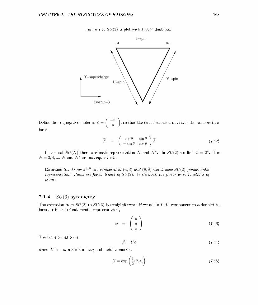
CHAPTER 7. THE STRUCTURE OF HADRONS 168
Figure 7.3: SU(3) triplet with I, U, V doublets.
Y−supercharge
isospin−3
I−spin
V−spinU−spin
Dene the conjugate doublet as φ =
(−np
), so that the transformation matrix is the same as that
for φ,
φ′ =
(cos θ sin θ− sin θ cos θ
)φ (7.42)
In general SU(N) there are basic representation N and N∗. In SU(2) we nd 2 = 2∗. ForN = 3, 4, ..., N and N∗ are not equivalent.
Exercise 51. Pions π±,0 are composed of (u, d) and (u, d) which obey SU(2) fundamentalrepresentation. Pions are avor triplet of SU(2). Write down the avor wave functions ofpions.
7.1.4 SU(3) symmetry
The extension from SU(2) to SU(3) is straightforward if we add a thrid component to a doublet toform a triplet in fundamental representation,
φ =
uds
(7.43)
The transformation isφ′ = Uφ (7.44)
where U is now a 3× 3 unitary unimodular matrix,
U = exp
(1
2iθiλi
)(7.45)

CHAPTER 7. THE STRUCTURE OF HADRONS 169
where λi are eight independent Hermitian traceless 3× 3 matrices analogous to the σi of SU(2). Wecan choose the form given by Gell-Mann,
λ1 =
0 1 01 0 00 0 0
, λ2 =
0 −i 0i 0 00 0 0
, λ3 =
1 0 00 −1 00 0 0
,
λ4 =
0 0 10 0 01 0 0
, λ5 =
0 0 −i0 0 0i 0 0
,
λ6 =
0 0 00 0 10 1 0
, λ7 =
0 0 00 0 −i0 i 0
, λ8 =1√3
1 0 00 1 00 0 −2
(7.46)
Normally we use Ti = 12λi. The SU(2) is subgroup of SU(3). The λ1,2 have the structure of SU(2)
in 12-block which is isospin subgroup. The λ6,7 have the same structure in 23-block which is calledU-spin. λ4,5 is related to V-spin. See gures for their relation. The SU(2) doublets are
u, d(I) d, s(U) u, s(V ) (7.47)
We can dene ladder operators from Ti for isospin, U-spin and V-spin,
I± = T1 ± iT2 =
0 1(0) 00(1) 0 0
0 0 0
U± = T6 ± iT7 =
0 0 00 0 1(0)0 0(1) 0
V± = T4 ± iT5 =
0 0 1(0)0 0 0
0(1) 0 0
(7.48)
They satisfy
[I+, I−] = 2I3 = diag(1,−1, 0)
[U+, U−] =3
2Y − I3 = 2U3 = diag(0, 1,−1)
[V+, V−] =3
2Y + I3 = 2V3 = diag(1, 0,−1) (7.49)
where I3 = T3 = 12λ3 is the isospin operator since acting on u, d, s it has eigenvalues ± 1
2 , 0 respectively.The hypercharge operator is
Y =2√3T8 =
1√3λ8 (7.50)
The Gell-Mann matrices satisfy the Lie algebra,
[Ti, Tj ] = ifijkTk (7.51)
with the anti-symmetric structure constants fijk given in Tab. 7.1. Also we have anti-commutator
Ti, Tj =1
3δij + dijkTk (7.52)
where symmetric structure constants dijk are given in Tab. 7.1.

CHAPTER 7. THE STRUCTURE OF HADRONS 170
Table 7.1: Structure constants of SU(3).
f123 = 1f147 = f246 = f257 = f345 = f516 = f637 = 1/2
f458 = f678 =√
3/2
d118 = d228 = d338 = −d888 = 1/√
3d146 = d157 = d256 = d344 = d355 = 1/2
d247 = d366 = d377 = −1/2
d448 = d558 = d668 = d778 = −1/(2√
3)
We can generalise these results by dening N × N matrices Ti which satisfy Eq. (7.51) andtransform N-dimensional states by
φ→ φ′ = (1 + iθiTi)φ (7.53)
These states form N-dimensional multiplets of SU(3).A SU(3) irreducible representation can be drawn in the I3 − Y diagram. We know that the
eigenvalues of I3 are 0,± 12 ,±1,± 3
2 , · · · , so are U3 and V3. From Y = 23 (U3 + V3), the eigenvalues of
hypercharge are 0,± 13 ,± 2
3 ,±1,± 43 , · · · . Then the basis vectors locate on the grid points with spacing
( 12 ,
13 ) for I3 and Y , see Fig. 7.4. The function of T± is to change I3 by ±1 while keeping Y xed.
The operator U± is to change (I3, Y ) by (∓ 12 ,±1), while V± is to change (I3, Y ) by (± 1
2 ,±1). Thereare three kinds of irreducible representation: (1) There is one point on (0, 0); (2) There is one pointon (0, 2
3 ); (3) There is one point on (0,− 23 ). As an example, the weight diagram for the irreducible
representation (p, q) = (4, 1) is shown in Fig. 7.6 and 7.5. Any SU(3) representation has a convexboundary in I3 − Y space. The maximum state φmax can be dened by
I+φmax = U+φmax = V+φmax = 0 (7.54)
Let I3(φmax) = p/2 and U3(φmax) = q/2, we obtain for φmax
(I3, Y ) =
(p
2,p+ 2q
3
)(7.55)
The maximum state φmax can also be dened in an alternative way,
I+φmax = U−φmax = V+φmax = 0 (7.56)
Then (I3z, Y ) for φmax is obtained by acting (U−)q on φmax given in Eq. (7.55), changing (I3, Y ) by(q/2,−q),
(I3, Y ) =
(p+ q
2,p− q
3
)(7.57)
Here we choose this φmax, see Fig. 7.6. We see that the maximum state φmax can be characterized bya pair of numbers (p, q). The SU(3) irreducible representation can be completely specied by a pair ofnumber (p, q), so we denote it as D(p, q), see Tab. (7.2). The maximum state is composed of p-quarksand q-antiquarks. We will see in the next section that the irreducible representation notation D(p, q)
corresponds to a irreducible tensor representation Ti1···ipa1···aq . The irreducible representation (p, q) can
be classied into three categories by,
c(p, q) = p+ 2q = (p− q) (mod 3) (7.58)
as: (1) c(p, q) = 0, C2 and C3 are integers, there is one point on (0, 0) in (I3, Y ) plot; (2) c(p, q) = ±1,C2 and C3 are fractions, there is one point on (0,− 2
3 ) and ( 23 , 0) respectively. If c(p, q) = −c(q, p),
where c(q, p) is the c-number for its conjugate representation.

CHAPTER 7. THE STRUCTURE OF HADRONS 171
Figure 7.4: (I3, Y ) gure and U±,V± and I±.
1 3/21/2 2−1/2−1−3/2−2−5/2 5/2
1/3
2/3
4/3
5/3
−1/3
−2/3
−4/3
−5/3
1
−1
Y−supercharge
I−spin+
U−spin+
U−spin−
V−spin+
V−spin−
I−spin+I−spin−
Figure 7.5: The irreducible representation (p, q) = (4, 1). The weight of the states in the outer layeris 1, while that of the states surrounded by circles in the inner layers is 2.
Y−supercharge
isospin−3
q*unit
q*unit
p*unit
p*unit

CHAPTER 7. THE STRUCTURE OF HADRONS 172
Figure 7.6: The maximum state φmax given in Eq. (7.57) for the octet, triplet and anti-triplet.
V−spin+
I−spin+
U−spin−
phi−max
Y−supercharge
isospin−3
Y−superchargeY−supercharge
triplet anti−tripletoctet
−one−half one−half
−two−third
−one−half one−half
two−third
one−third
−one−third
s−quark
anti−s−quark
phi−max
isospin−3 isospin−3phi−max
anti−d−quarkanti−u−quark
d−quark u−quark
The irreducible representation D(p, q) can also be expressed by the Young tableaux as shown inFig. 7.7.
There are two Casimir operators, C2 and C3 in SU(3). The quadratic Casimir operator C2 isdened by
C2 =∑i
T 2i =
1
2I+, I−+ I2
3 +1
2U+, U−+
1
2V+, V−+ T 2
8 (7.59)
We can compute the magnitude of the Casimir operator for any SU(3) representation by acting withC2 on the maximal state of that representation. We can rewrite C2 by moving I+, V+ and U− are tothe right side of any pair of operators
C2 =1
2I+, I−+ I2
3 +1
2U+, U−+
1
2V+, V−+ T 2
8
= I−I+ + I3 + I23 + U+U− − U3 + V−V+ + V3 + T 2
8
= I23 + 2I3 + I−I+ + U+U− + V−V+ +
3
4Y 2 (7.60)
So we get
〈φmax|C2|φmax〉 =⟨I23
⟩+ 2 〈I3〉+
3
4Y 2 (7.61)
Then C2 for D(p, q) becomes
C2 =1
3(p2 + pq + q2) + (p+ q) (7.62)
We see that C2 is symmetric with respect to exchanging p and q. The values of C2 for some repre-sentations are listed in Tab. (7.2).
The cubic Casimir operator C3 is dened by
C3 = −ifi1j1j2ifi2j2j3ifi3j3j1Ti1Ti2Ti3 = −[Tj1 , Tj2 ][Tj2 , Tj3 ][Tj3 , Tj1 ] (7.63)
The eigenvalue of C3 for the representation (p, q) is given by
C3 = (p+ 2q)(p+ 2)− 1
9(p− q)(2p2 + 5pq + 2q2) (7.64)

CHAPTER 7. THE STRUCTURE OF HADRONS 173
Table 7.2: Irreducible representations for SU(3).
tensor rank dimension C2
T i (1,0) 3 4/3Ta (0,1) 3 4/3T ia (1,1) 8 3T ij (2,0) 6 10/3Tab (0,2) 6 10/3T ijk (3,0) 10 6Tabc (0,3) 10 6
T ijab (2,2) 27 8
We see that C3 assumes dierent values for conjugate representation, i.e. it is not symmetric for pand q.
The commutation rule for SU(N) generators is given by,
[Gi, Gj ] = ifijkGk, (7.65)
where i, j, k = 1, ...,M . The coecients fijk are the structure constants of SU(N). There alwaysexists a M-dimensional representation, the so-called regular representation or adjoint representationdened by the structure constants,
(Gi)jk = −ifijk. (7.66)
One can prove that the above matrices in Eq. (7.66) satisfy the commutation rule (7.65) by usingthe Jacobi's identity,
[[Gi, Gj ], Gk] + [[Gj , Gk], Gi] + [[Gk, Gi], Gj ] = 0 (7.67)
Exercise 52. Prove the Casimir operator C2 is commutable with all Gell-Mann matrices Ti(i = 1, · · · , 8), [C2, Ti] = 0.
7.1.5 Tensor representation of SU(3)
See Ref. [16]. Corresponding to the (n,m) irreducible representation, we have a (n,m) tensor T i1···ina1···amtransforming under SU(3),
T i1···ina1···am → U i1j1 · · ·UinjnU+b1a1 · · ·U+bm
am T j1···jnb1···bm (7.68)
There are three special tensors.(1) δij is a (1,1) tensor.
δij → U ii1U+j1j δi1j1 = (UU+)ij = δij (7.69)
(2) εijk is a (3,0) tensor. εijk is a (0,3) tensor.
εijk → U ii1Ujj1Ukk1ε
i1j1k1 = εijkdetU = εijk (7.70)

CHAPTER 7. THE STRUCTURE OF HADRONS 174
Using δij , εijk and εijk, we can form dierent tensors from T i1···ina1···am ,
Ai2···ina2···am = δi1a1Ti1···ina1···am ,
Bi3···inba1···am = εbi1i2Ti1i2i3···ina1···am ,
Cbi1···ina3···am = εba1a2T i1···ina1a2a3···am , (7.71)
where A, B and C are (n− 1,m− 1), (n− 2,m + 1) and (n + 1,m− 2) tensors respectively if theyare not zero. We say that T i1···ina1···am is reducible.
A irreducible (n,m) tensor T i1···ina1···am has following properties: (1) Symmetric under interchange ofany two subscript and superscript indices; (2) Contraction of any one superscript and one subscriptindices gives zero.
An irreducible (n,m) tensor T i1···ina1···am form a basis for the irreducible representation of SU(3). Thedimension of the representation is given by
d = (1 + n)(1 +m)[1 + (n+m)/2]. (7.72)
Now we give a proof. We rst focus on the upper indices. Due to the symmetry, the order of theindices is irrelevant. Suppose we put the indices in such an order: ones, twos and threes. If there arej ones, and then (n − j) twos and threes. There are (n − j + 1) combinations in this case. In totalthe number of dierent components is then
n∑j=0
(n− j + 1) =1
2(n+ 1)(n+ 2) (7.73)
Similarly for lower indices there are 12 (m+ 1)(m+ 2) linearly independent components. So a (n,m)
tensor has 14 (m + 1)(m + 2)(n + 1)(n + 2) independent components. The trace of the tensor is a
(n− 1,m− 1). The traceless requirement leads to 14m(m+ 1)n(n+ 1) conditions. The dimension of
the irreducible representation is then
d =1
4(m+ 1)(m+ 2)(n+ 1)(n+ 2)− 1
4m(m+ 1)n(n+ 1)
=1
2(m+ 1)(n+ 1)(m+ n+ 2) (7.74)
Suppose Aij andBij are two irreducible (1,1) tensors (octet), so they are traceless. We can construct
a (2,2) tensor T ijab = AiaBjb which can be reduced to tensors in Tab. (7.3). For example the 27-plet is
T ijab = AiaBjb +AibB
ja +AjaB
ib +AjbB
ia − δia(AcbB
jc +AjcB
cb)− δja(AicB
cb +AcbB
ic)
−δib(AcaBjc +AjcBca)− δjb(AicBca +AcaB
ic) (7.75)
Exercise 53. Consider the tensor decomposition of D(2, 0)⊗D(0, 2).
7.1.6 Reduction of direct product of irreducible representations in SU(3)
There are many ways to reduce the direct product of two irreducible representations. Here we takeYoung tableaux method as an example. As we have learned that an IR representation D(p, q) can berepresented by a Young table with the rst and second rows to have p+ q and q boxes, as shown inFig. 7.7. The dimension of the representation is given in Eq. (7.72). Consider the following reductionD(3, 1)⊗D(1, 1). The procedure is (1) Fix the rst one D(3, 1), label each box of D(1, 1) by its rownumber; (2) Move each box from D(1, 1) to D(3, 1) one by one; (3) For the labelled boxes which are in

CHAPTER 7. THE STRUCTURE OF HADRONS 175
Table 7.3: Irreducible tensor from T ijab = AiaBjb .
tensor rank dimS = AiaB
ai (0,0) 1
F ia = AijBja −BijAja (1,1) 8
Dia = AijB
ja +BijA
ja − 2
3δijS (1,1) 8
AiaBjbεabk+all permutations of (i,j,k) (3,0) 10
AiaBjbεijc+all permutations of (a,b,c) (0,3) 10
AiaBjb+symmetric term-(trace) (2,2) 27
the same row, the order of numbers from the left to the right should not decrease (equal or increase);(4) For the labelled boxes which are in the same column, the numbers should be all dierent, andshould increase from up to down; (5) Counting labelled boxes from up-right to down-left, the numberof boxes labelled by 1 should be no less than that labelled by 2 in each step of the counting. (6)Delete any column with 3 or more boxes.
The result of the reduction is then,
D(3, 1)⊗D(1, 1) = D(4, 2)⊕D(5, 0)⊕D(2, 3)⊕D(3, 1)⊕D(3, 1)⊕D(2, 0) (7.76)
The dimension of an IR representation D(p, q) can also be computed by using the Young tableaux.The dimension is gven by d1/d2 where d1 and d2 are products of two series of numbers lled in eachbox of the Young tableaux. The rule of the lling for d1 is: (1) ll one number in each box; (2)ll 3 [for SU(3)] in the upper-left box; (3) the number increases by 1 when moving to the right anddecreases by 1 when moving to down. The rule for d2 is: ll one number in each box, which is thenumber of boxes counting from this box to its right end plus that to its lower end and minus 1. Forexample, we can compute the dimension of D(1, 1) = 8 according to this rule, see Fig. 7.8.
Exercise 54. Consider the decomposition of D(3, 2)⊗D(2, 1) in Young tableaux.
7.1.7 Quarks as building blocks for hadrons
According to the quark model, all hadrons are made up of a small variety of more basic entities, calledquarks, bound together in dierent ways. The fundamental representation of SU(3), the multipletfrom which all other multiplets can be built, is a triplet. There are also anti-quark multiplets inwhich the signs of additive quantum numbers are reversed. Each quark is assigned spin 1/2 andbaryon number B = 1/3. See Fig. (7.6). Baryons are made of three quarks (qqq) and mesons ofquark-anti-quark (qq). A new additive quantum number is called the hypercharge, i.e. the sum ofthe baryon number and the strangeness number,
Y = B + S (7.77)
The charge, Qe, is given by the Gell-mann-Nishijima relation,
Q = I3 +Y
2(7.78)
The quantum number of the quarks are listed in Tab. (7.4).

CHAPTER 7. THE STRUCTURE OF HADRONS 176
Figure 7.7: Young tableaux and reduction of the direct product.
1 1 1
1
1
1
1
1
1 1 1 1 1
1 2
1
1
2
1
1
1
1
1 1
p−box
q−box
(p , q) IR rep............
......
2
1 1
2
2
2
2
times
D(4,2) D(5,0) D(2,3) D(3,1) D(3,1) D(2,0)
1 1
2
Figure 7.8: The dimension of D(3, 1).
3 4 5 6
2
5 3 2 1
1
24
Table 7.4: Quantum numbers of the quarks.
quark spin B Q I3 S Yu 1/2 1/3 2/3 1/2 0 1/3d 1/2 1/3 -1/3 -1/2 0 1/3s 1/2 1/3 -1/3 0 -1 -2/3

CHAPTER 7. THE STRUCTURE OF HADRONS 177
7.1.8 Mesons as quark-anti-quark states
In the quark model, mesons are bound states made of a quark and an anti-quark. Consider two avorcase, q = (u, d), q = (−d, u), the mesons are in isotriplet and isosinglet, i.e. [2] ⊗ [2] = [3] ⊕ 1 inSU(2),
|I = 1, I3 = 1〉 = −ud
|I = 1, I3 = 0〉 =1√2
(uu− dd)
|I = 1, I3 = −1〉 = du
|I = 0, I3 = 0〉 =1√2
(uu+ dd) (7.79)
They are pions: π+ = ud (we neglect the minus sign), π− = du and π0 = 1√2(uu− dd). The masses
of pion are about: 140 MeV (π±) and 135 MeV (π0). The spin, parity and C-parity of pions areJPC = 0−+. The isospin scalar 1√
2(uu+ dd) will be mixed with other I3 = Y = 0 states.
For three avor case, q = (u, d, s), q = (u, d, s), there are nine possible combinations. See Fig.(7.9) for resulting meson nonet. The nine states divide into an SU(3) octet and an SU(3) singlet.The decomposition can be written as
[3]⊗ [3∗] = [8]⊕ [1]
D(1, 0)⊗D(0, 1) = D(1, 1)⊕D(0, 0) (7.80)
Three states, A, B and C, have I3 = Y = 0. These are linear combinations of uu, dd, and ss states.The singlet combination, C, must contain each quark avor on an equal footing, so we have
C =1√3
(uu+ dd+ ss) (7.81)
State A is taken to be a member of the isospin triplet (du,A,−ud) and so we have
A =1√2
(uu− dd) (7.82)
By orthogonality to A and C, we can nd B,
B =1√6
(uu+ dd− 2ss) (7.83)
We often use the notation (SU(3),SU(2)),
A = π0, ρ0([8], [3])
B = η8, ω8([8], [1])
C = η1, ω1([1], [1]) (7.84)
The physical η and η′ or ω and φ are mixtures of η1,8 and ω1,8 respectively. The η and η′ are almostoctet and singlet respectively,
η ≈ η8 =1√6
(uu+ dd− 2ss),
η′ ≈ η1 =1√3
(uu+ dd+ ss).

CHAPTER 7. THE STRUCTURE OF HADRONS 178
Here are their masses and spin-parities: η(548) and η′(958), JPC = 0−+. The physical ω and φappear to be ideal mixture:
φ =1√3ω1 −
√2
3ω8 = ss
ω =
√2
3ω1 +
1√3ω8 =
1√2
(uu+ dd) (7.85)
Their masses and spin-parities are φ(1020), ω(1420), JPC = 1−−.Octet mesons can be expressed by
[8] → M = qaqb −1
3δab q
cqc (7.86)
where qi is the quark eld and qi is its Hermite conjugation (antiquark). Under the SU(3) transfor-mation q → Uq, the meson tensor transforms as
M → UMU+ (7.87)
Matrix form
M =
π0√
2+ η8√
6π+ K+
π− − π0√
2+ η8√
6K0
K− K0 − 2√
6η8
=1√2ξaλa (7.88)
where
π± =1√2
(ξ1 ∓ iξ2), π0 = ξ3
K± =1√2
(ξ4 ∓ iξ5), K0/K0
=1√2
(ξ6 ∓ iξ7)
η8 = ξ8 (7.89)
The singlet can be written as
[1] → S =1
3δab q
cqc =η1√
3
1 0 00 1 00 0 1
(7.90)
One can verify
M + S =
π0√
2+ η8√
6+ η1√
3π+ K+
π− − π0√
2+ η8√
6+ η1√
3K0
K− K0 − 2√
6η8 + η1√
3
=
uds
(u, d, s) =
uu ud us
du dd ds
su sd ss
(7.91)
Here are masses and spin-parity for kaons: K±(494), K0(498) and K0(498), JP = 0−.
Like any quantum-mechanical bound system, the qq pair will have a discretre energy level spectrumcorresponding to the dierent modes of qq excitations. The intrinsic spin of qq is S = 0, 1. The spin

CHAPTER 7. THE STRUCTURE OF HADRONS 179
Figure 7.9: Meson nonet as qq bound states. A,B,C are states with Y = I3 = 0 composed ofuu, dd, ss.
C
ud
dsbar usbar
dubar
subar sdbar
udbar
s
A
B
Table 7.5: Some examples of JP (spin-parity) about meson multiplets (nonets). We have usedabbreviation S=scalar,PS=pseudoscalar, V=vector, AV=axial vector, T=tensor, AT=axialtensor.
multiplets S PS V AV T ATJP 0+ 0− 1− 1+ 2+ 2−
J of the composite meson is the vector sum of this spin and the relative orbital angular momentumL of the q and q. The parity of the meson is,
P = (−1)L+1 (7.92)
where the minus sign arises because the q and q have opposite intrinsic parity, and (−1)L arises fromthe space inversion replacements θ → π − θ, φ → π + φ in the angular part of the qq wavefunctionYLM (θ, φ). A neutral qq system is an eigenstate of the particle-anti-particle conjugation operatorC. The value of C can be deduced by q ↔ q and then interchanging their positions and spins. Thecombined operation gives
C = −(−1)S+1(−1)L = (−1)L+S (7.93)
where the minus sign arises from interchanging fermions, the (−1)S+1 from the symmetry of the qqspin states, and the (−1)L from the angular momentum. Here S is the total intrinsic spin of the qqpair. The total meson spin J is given by |L− S| < J < |L+ S|.
The C-parity is only dened for neutral particles or systems. Now we extend the C-partity byintroducing the G-partity which is not limited to neutral systems or particles. The ud state can be
Table 7.6: Some examples of JPC (spin-parity-C-parity) about ground state (L = 0) and rst excited(L = 1) mesons. We have used abbreviation PS=pseudoscalar, V=vector, S=scalar, AV=axialvector, T=tensor.
multiplets PS (L = 0) V (L = 0) S (L = 1) AV (L = 1) T (L = 1)JPC 0−+ 1−− 0++ 1++, 1+− 2++

CHAPTER 7. THE STRUCTURE OF HADRONS 180
Figure 7.10: Pseudoscalar (JP = 0−) and vector mesons (JP = 1−).
dsbar usbar
dubar
subar sdbar
udbar
octet−triplet
octet−singletsinglet−singlet
pseudoscalar
dsbar1 usbar1
dubar1
subar1 sdbar1
udbar1
octet−triplet1
octet−singlet1singlet−singlet1
vector
either symmetric or anti-symmetric
φS =1√2
(ud+ du)
φA =1√2
(ud− du)
These states are distinguished by G-parity dened by
G = Ciτ2 = C
(0 1−1 0
)where C is the charge conjugation operator. Let's see
G
(ud
)= C
(0 1−1 0
)(ud
)= C
(d−u
)=
(d−u
)G
(d−u
)= G2
(ud
)= −
(ud
)so we have
GφS =1√2G(ud+ du) = − 1√
2(du+ ud) = −φS
GφA =1√2G(ud− du) =
1√2
(−du+ ud) = φA
We can see
π0 ∼ 1
2[(uu− dd) + (uu− dd)] = φ0
S
ρ0 ∼ 1
2[(uu− dd)− (uu− dd)] = φ0
A
This denition is consistent to the fact about the C-parity,
Cφ0S = φ0
S , Cφ0A = −φ0
A

CHAPTER 7. THE STRUCTURE OF HADRONS 181
Table 7.7: qq representations with explicit G-parity
K+(K+∗) 1√2(us± su)
K0(K0∗) 1√2(ds± sd)
K−(K−∗) 1√2(su± us)
K0(K
0∗) − 1√
2(sd± ds)
π+(ρ+) − 1√2(ud± du)
π−(ρ−) 1√2(du± ud)
π0(ρ0) 12 [(uu− dd)± (uu− dd)]
η08(ω0
8) 12√
3[(uu+ dd− 2ss)± (uu+ dd− 2ss)]
η01(ω0
1) 1√6[(uu+ dd+ ss)± (uu+ dd+ ss)]
Therefore 0− mesons (pseudoscalar) are the symmetric states with negative G-parity, while 1− mesons(vector) are anti-symmetric states with positive G-parity.
Combining with spins, we have following possibilities for the symmetry property of SU(3)-SU(2)wave function φχ under the interchange of 1 and 2,
symmetric : φSχS , φAχA
anti− symmetric : φSχA, φSχA
where χA denotes the spin single wave function and χS the triplet wave function. The 0− and 1−
mesons are totally anti-symmetric because the wave functions for neutral particles are
π0 ∼ φ0SχA
ρ0 ∼ φ0AχS
Hence the wave functions for the 0− mesons are φSχA while that for the 1− mesons are φAχS .
7.1.9 Baryons as three-quark states
A baryon is a bound state of three quarks. First we combine two quarks,
[3]⊗ [3] = [6]⊕ [3] (7.94)
Then the third one,
([3]⊗ [3])⊗ [3] = ([6]⊕ [3])⊗ [3] = [6]⊗ [3] + [3]⊗ [3]
= [10]⊕ [8]MS ⊕ [8]MA ⊕ [1] (7.95)
where 'MS' and 'MA' mean mixed symmetric and mixed anti-symmetric SU(3) multiplets. As anexample, we construct 'uud' whose combinations are denoted as ∆, pMS , and pMA. Combining thenon-strange member of the [3] with the u quark of the [3], we have
pMA =1√2
(ud− du)u (7.96)
Note that (ud − du) behaves like a s in SU(3)f . The decuplet states are totally symmetric underinterchange of quarks, as evidenced by the uuu, ddd, and sss members. The symmetric combinationof 'uud' is
∆ =1√3
[udu+ duu+ uud] (7.97)

CHAPTER 7. THE STRUCTURE OF HADRONS 182
Requiring orthogonality of the remaining 'uud' state to both pMA and ∆ gives
pMS =1√6
[(ud+ du)u− 2uud] (7.98)
The states pMS and pMA have mixed symmetry, they are analogous to∣∣ 1
2 ,± 12
⟩MA
in Eq. (7.33) and∣∣ 12 ,± 1
2
⟩MS
Eq. (7.34). The quark structure of other states can be readily obtained in a similar wayby using U or V spin. The singlet is (Problem: prove this)
(qqq)[1] =1√6
[u(ds− sd) + s(ud− du) + d(su− us)]
v1√6
[uu+ ss+ dd] (7.99)
The reduction of direct product of three spin-1/2 states is given in Eq. (7.30). The spin statesare displayed in Eq. (7.32)-(7.34). The two doublets have mixed symmetry that the spin states aresymmetric or anti-symmetric with interchange of two quarks. We can label states by (SU(3),SU(2)),
S : ([10], [4]) + ([8], [2])
MS : ([10], [2]) + ([8], [4]) + ([8], [2]) + ([1], [2])
MA : ([10], [2]) + ([8], [4]) + ([8], [2]) + ([1], [2])
A : ([1], [4]) + ([8], [2]) (7.100)
The ground state baryons t into the JP = (3/2)+ decuplet and the JP = (1/2)+ octet. See Fig.7.13. Their spatial wave functions are symmetric, belonging to the S wave (L = 0) in orbital agularmomentum. Their spin and avor or SU(6) wavefunctions are totally symmetric. The total wavefunctions for ground state baryons must be anti-symmetric. Then a new degree of freedom for quarks,whose wave function is anti-symmetric, is needed for ground state baryons (and for all baryons). Thisnew degree of freedom is called the color. We will discuss it in Section 7.2. The decuplet and octetground state baryons belong to ([10], [4]) and ([8], [2]) respectively. For example, the wave functionof spin-up proton is∣∣∣∣p, Jz =
1
2
⟩=
1√2
[pMS
∣∣∣∣12 , 1
2
⟩MS
+ pMA
∣∣∣∣12 , 1
2
⟩MA
]=
1√18
1
2(udu+ duu− 2uud)(↑↓↑ + ↓↑↑ −2 ↑↑↓)
+3
2(udu− duu)(↑↓↑ − ↓↑↑)
=
1√18udu(2 ↑↓↑ − ↑↑↓ − ↓↑↑) + duu(2 ↓↑↑ − ↑↑↓ − ↑↓↑)
+ uud(2 ↑↑↓ − ↑↓↑ − ↓↑↑) (7.101)
where spin wave functions∣∣ 1
2 ,12
⟩MA,MS
are given by Eq.(7.33,7.34).
A simple way to get the spin-avor wave functions is to start from the simplest known wavefunctions of certain baryons and to use the spin ladder operators. For example, staring from∣∣∣∣∆+, Jz =
3
2
⟩=
1√3P(|u ↑, u ↑, d ↑〉)
=1√3
(|u ↑, u ↑, d ↑〉+ |u ↑, d ↑, u ↑〉+ |d ↑, u ↑, u ↑〉) (7.102)

CHAPTER 7. THE STRUCTURE OF HADRONS 183
where P(|u ↑, u ↑, d ↑〉) is to sum over all dierent permutations, we can derive∣∣∆+, Jz = 1
2
⟩by using
the spin ladder operator S− = s1− + s2− + s3−,∣∣∣∣∆+, Jz =1
2
⟩= S−
∣∣∣∣∆+, Jz =3
2
⟩=
1√3
(s1− + s2− + s3−)(|u ↑, u ↑, d ↑〉+ |u ↑, d ↑, u ↑〉+ |d ↑, u ↑, u ↑〉)
=1
2√
3|u ↓, u ↑, d ↑〉+ |u ↓, d ↑, u ↑〉+ |d ↓, u ↑, u ↑〉
+ |u ↑, u ↓, d ↑〉+ |u ↑, d ↓, u ↑〉+ |d ↑, u ↓, u ↑〉|u ↑, u ↑, d ↓〉+ |u ↑, d ↑, u ↓〉+ |d ↑, u ↑, u ↓〉
→ 1
3[P(|u ↓, u ↑, d ↑〉) + P(|u ↑, u ↓, d ↑〉) + P(|u ↑, u ↑, d ↓〉)] (7.103)
One can verify that the spin-up proton is the orthogonal state to∣∣∆+, Jz = 1
2
⟩with the same values
of I3 and Sz.
Exercise 55. Write down the spin-avor wave functions for the ground state decuplet (3/2)+
and octet (1/2)+ baryons, and show that they are totally symmetric under the interchangeof two quark labels. The decuplet (3/2)+ and octet (1/2)+ baryons are shown in the left andright panel of Fig. 7.13 respectively.
Exercise 56. Starting from∣∣Σ∗+, Jz = 3
2
⟩= |u ↑, u ↑, s ↑〉, nd the spin-isospin function of∣∣Σ0, Jz = 1
2
⟩and
∣∣Λ, J = 12
⟩.
Exercise 57. For a non-relativistic particle with the charge Q and the mass m, its magneticmoment is given by,
µ =Q
2mgs (7.104)
where g = 2 is the g-factor for elementary particles. We know that the magnetic moment ofa proton (neutron) is µp = 2.79µN (µn = −1.91µN ) with µN = e
2mpthe nuclear magneton,
which corresponds to gp = 5.6 (gn = −3.82). Since the neutron is a neutral particle, itsmagnetic moment indicates that it is made of electrically charged particles: quarks. Showthe following relation with the wave functions of proton and neutron,⟨
p, 12
∣∣µzp∣∣ p, 12
⟩⟨n, 1
2 |µzn|n, 12
⟩ = −3
2(7.105)
where
µzp,n =gq
2mq
3∑i=1
Qisiz
where gq = 2, mq and Qi are the g-factor, mass and charges for quarks.

CHAPTER 7. THE STRUCTURE OF HADRONS 184
Figure 7.11: The qq multiplet of SU(3). 3⊗ 3 = 6⊕ 3.
u
s
dd uusextet_ud
sextet_ds sextet_us
triplet_ud
d
ss
Figure 7.12: The qqq multiplet of SU(3). 3⊗ 3⊗ 3 = 10⊕ 8⊕ 8⊕ 1.
dd uu
ss

CHAPTER 7. THE STRUCTURE OF HADRONS 185
Figure 7.13: Ground state baryons, the decuplet [JP = (3/2)+] and octet [JP = (1/2)+].
delta−1232
sigma−star−1385
xi−1530
omega−1672
Jp=3/2+
neutron proton
sigma− sigma+sigma0
lambda
xi− xi0
Jp=1/2+
7.1.10 Gell-Mann-Okubo relations
Similarly as in Eq. (7.88), the avor contents of the baryon and anti-baryon octets can also be writtenas
B =
Σ0√
2+ Λ√
6Σ+ p
Σ− −Σ0√
2+ Λ√
6n
Ξ− Ξ0 − 2√6Λ
B =
Σ
0
√2
+ Λ√6
Σ−
Ξ−
Σ+ −Σ
0
√2
+ Λ√6
Ξ0
p n − 2√6Λ
(7.106)
It can be proved that Bij can also be written in the form,
Bij ∼ qiqaqbεabj −1
3δijq
kqaqbεabk
The baryons and anti-baryons transform in SU(3) as
B → UBU+
B → UBU+ (7.107)
We can write the strong Hamiltonian as
H = Hsys +Hasym (7.108)
where Hsys is invariant under SU(3) transfromation. The SU(3) violated term is denoted by Hasym.To make the baryon number conserve in Hasym, Hasym has to be in the bilinear form (as it gives themasses of baryons) and traceless in avor indices,
Sji ∼ qiγ0qj − 1
3δji qiγ0q
j ∼ ψ†i γ0ψj −1
3δjiψ†kγ0ψk (7.109)

CHAPTER 7. THE STRUCTURE OF HADRONS 186
where qi ∼ ψi and qi ∼ ψ†i with ψi and ψ†i spinors and i the avor index. Assume that Hasym Hsys,so Hasym can be regarded as perturbation. Suppose |h〉 is the eigenstate of Hsys,
Hsys |h〉 = γ |h〉 (7.110)
So the energy expectation value becomes
Eh ≈ γ + 〈h |Hasym|h〉 (7.111)
Let's determine the form of 〈h |Hasym|h〉. Note that |h〉 are eigenstates of Hsys and belong to therepresentation of SU(3). The matrix 〈h |Hasym|h〉 can be regarded as the transition amplitude of theprocess
h → h+ Sij (7.112)
where Sij is the pseudoparticle which belongs to SU(3) octet. Let's discuss a speical case Sij = S3
3δi3δj3.
Denote |h〉 = Bij , the gedanken process is
Bij → Bab + S33 (7.113)
The perturbation Hasym can be regarded as formed by three octets, Bij , Ba
b and Sij ,
Hasysm ∼ (αBi
aBaj + βB
a
jBia)Sji ∼ αB
3
aBa3 + βB
a
3B3a
= α(pp+ nn+2
3ΛΛ) + β(Ξ
−Ξ− + Ξ
0Ξ0 +
2
3ΛΛ)
= α(pp+ nn) + β(Ξ−
Ξ− + Ξ0Ξ0) +
2
3(α+ β)ΛΛ (7.114)
The total energy is then
Eh ≈ γ + α(pp+ nn) + β(Ξ−
Ξ− + Ξ0Ξ0) +
2
3(α+ β)ΛΛ (7.115)
We can derive
EΣ = γ
EΛ − EΣ =2
3(α+ β)
EN − EΣ = α
EΞ − EΣ = β (7.116)
So we derive
3(EΛ − EΣ) = 2(EN − EΣ) + 2(EΞ − EΣ) (7.117)
which becomes
3EΛ + EΣ − 2EN − 2EΞ = 0 (7.118)
The above relation can be transformed into that of mesons by replacing Λ→ η, N → K, Ξ→ K,
3Eη + Eπ − 4EK = 0 (7.119)
The above relatons can be casted into ultra-relativistic case, where
Ei =√p2 +m2
i ∼ p+m2i
2p(7.120)

CHAPTER 7. THE STRUCTURE OF HADRONS 187
Table 7.8: Masses of octet baryons and mesons. Unit=MeV.
N 939 π 140
Λ 1116 K,K 495Σ 1192 η 549Ξ 1315
The above equations become
3m2Λ +m2
Σ − 2m2N − 2m2
Ξ = 0
3m2η +m2
π − 4m2K = 0 (7.121)
Here we have assumed that |h〉 is a state with momentum p mi. For non-relativistic case we have
3mΛ +mΣ − 2mN − 2mΞ = 0
3mη +mπ − 4mK = 0 (7.122)
We can check the above relations (7.121) and (7.122) by inserting baryon and meson masses given inTable (7.8).
The baryon decuplet can be expressed by,
Bijk =1
n
∑P
qP (i)qP (j)qP (k) (7.123)
where the sum is over all dierent permutations and n is its number. The normalized state is givenby
1√n
∑P
qP (i)qP (j)qP (k) (7.124)
Then we have, e.g.
B333 = Ω
B133 =1√3
Ξ∗0
B113 =1√3
Σ∗+
B123 =1√6
Σ∗0 (7.125)
For the baryon decuplet, the mass formula can be derived in a similar way. The virtual process canbe written by
Blmn → Babc + Sij (7.126)
where we also take Sij = S33δi3δj3. The SU(3) violated Hamiltonian is then in the form,
Hasysm ∼(BiabB
jab − 1
3δjiBdabB
dab
)Sij ∼ β
(B3abB
3ab − 1
3BdabB
dab
)(7.127)

CHAPTER 7. THE STRUCTURE OF HADRONS 188
The total energy is
Eh ∼ α+ β
(B3abB
3ab − 1
3BdabB
dab
)= α+ β
[2
3ΩΩ +
1
3(Ξ∗0
Ξ∗0 + Ξ∗−
Ξ∗−)
−1
3(∆
++∆++ + ∆
+∆+ + ∆
0∆0 + ∆
−∆−)
](7.128)
This gives the result that the masses of isospin multiplets ∆, Σ∗, Ξ∗ and Ω are equal-distant,
mΣ∗ −m∆ = mΞ∗ −mΣ∗ = mΩ −mΞ∗ =β
3(7.129)
One can check the above formula by inserting the mass values of the decuplet baryons. Eq. (7.121),(7.122) and (7.129) can be summarized into the so-called Gell-Mann-Okubo relations [17, 18],
m = a+ bY + c
[I(I + 1)− 1
4Y 2
](7.130)
Exercise 58. Use the Gell-Mann-Okubo mass formula to obtain the masses of ground statebaryons, (1/2)+ and (3/2)+.
Exercise 59. We can dene a matrix in terms of meseon octet in Eq. (7.88) U = eiξaλa/f ,where λa are Gell-Mann matrices in Eq. (7.46), ξa are meson elds given in Eq. (7.89),and f is a constant. Then the Lagrangian due to the quark masses is given by
Lm ∼ f2
4
Tr[M(U + U†)]
(7.131)
where M = diag(mu,md,ms) is the quark mass matrix. Derive the masses for the mesonsby extracting the coecients of quadratic terms of mesonic elds.
7.2 Quarks and gluons
7.2.1 Color degrees of freedom
There are many evidences for the existence of color degree of freedom. We only take some of themas examples.
The rst one is from the baryons Ω(sss), ∆++(uuu) and ∆−(ddd) with the same avor content.We know that they belong to the ground state with orbital angular momentum L = 0, whose wavefunction is symmetric. The avor wave function is also symmetric. This seems to violate the Paulingprinciple for a fermionic system. So quarks must carry another degree of freedom - color. There arethree colors, R, G and B which makes a color triplet. The color wave function for three quarks shouldbe a color singlet which is anti-symmetric,
(qqq)[1] = [(RB −BR)G+ (BG−GB)R+ (GR−RG)B]/√
6 (7.132)
By the way, the color wave function for mesons is
(qq)[1] = (RR+GG+BB)/√
3 (7.133)

CHAPTER 7. THE STRUCTURE OF HADRONS 189
Figure 7.14: The denition of the R factor.
2electron
positron
gamma−z0 charge−quark
anti−quark−i
quark−i
2
positron
electron
gamma−z0
mu+
mu−
R =
Σflavor
The second evidence is the R factor dened by
R =σ(e+e− → qq → hadrons)
σ(e+e− → µ+µ−)(7.134)
Both reactions are electromagnetic interactions. Both quarks and electrons are pointlike particles.The only dierences are that muons carry unit charges, while quarks carry fractional charges, avorsand colors. The number of colors can be determined by measuring R. The factor can be written as
R = Nc∑f
Q2f (7.135)
where Qf is the quark electric charge for avor f and Nc the number of colors. In the energy rangewhere only light quarks (u, d, s) are produced, R = 2
3Nc. When the charm quark threshold is reached,the factor becomes R = 10
9 Nc. When the bottom quark is produced, we have R = 119 Nc. All these
values can be compared to data which show a clear evidence for Nc = 3.The third evidence is the decay rate of π0 → γ + γ, see Fig. 7.16. for illustration. The rate is
given by
Γ(π0 → 2γ) = N2c (Q2
u −Q2d)
2 α2m2
π
64π3f2π
(7.136)
where α = e2/4π = 1/137, Nc is the number of colors, mπ is the mass of neutral pion, Qu,d arecharges of u and d quarks, fπ is the pion decay constant for π → µν. We can estimate the rate bysubstituting Nc = 3, Qu = 2/3, Qd = 1/3, mπ = 140 MeV and fπ = 91 MeV,
Γ(π0 → 2γ) ≈ 9× 1
9
1
1372
1
64π3
(140
91
)2
MeV ≈ 7.6 eV (7.137)
which agree with the date very well,
Γexp(π0 → 2γ) = 7.48± 0.33 eV (7.138)
If quarks carry no color, the measured decay rate in experiments is about 9 times larger than thetheoretical prediction.
Color degrees of freedom respect SU(3)c symmetry. Unlike avor SU(3)f which is an approxi-mated symmetry, this is an exact symmetry and has dynamic eects.

CHAPTER 7. THE STRUCTURE OF HADRONS 190
Figure 7.15: The data for R [19].
Figure 7.16: Pions decay to two photons via axial vector current.
pion−zero
ax−vec
gamma−photon
gamma−photoncurrent

CHAPTER 7. THE STRUCTURE OF HADRONS 191
Table 7.9: Part of color factors c for one gluon exchange. Ti = λi/2 with λi the Gell-Mann matricesin Eq. (7.46).
initial nal gluon color factor cBB BB A8 (T8)33(T8)33 = 1
3
RR RR A3, A8 (T3)11(T3)11 + (T8)11(T8)11 = 13
RB RB A8 (T8)11(T8)33 = − 16
RB BR A4.A5 (T4)31(T4)13 + (T5)31(T5)13 = 12
BB BB A8 −(T8)33(T8)33 = − 13
BB RR A4, A5 −(T4)31(T4)13 − (T5)31(T5)13 = − 12
BB GG A6.A7 −(T6)23(T6)32 − (T7)23(T7)32 = − 12
7.2.2 Gluons as color carriers
The color interaction between quarks are carried by gluons. Gluons carry colors and anti-colors andbelong to a color octet. According to group theory, [3] ⊗ [3] = [1] ⊕ [8], the direct product of twotriplets can be reduced to a singlet and a octet. The gluon octet can be represented by gi (i = 1, ..., 8), R
GB
(R,G,B) =
13 (2RR−GG−BB) RG RB
GR 13 (2GG−RR−BB) GB
BR BG 13 (2BB −RR−GG)
+
1
3(RR+GG+BB)
1 0 00 1 00 0 1
=
A3√
2+ A8√
6A1−iA2√
2A4−iA5√
2A1+iA2√
2−A3√
2+ A8√
6A6−iA7√
2A4+iA5√
2A6+iA7√
2− 2A8√
6
+1√3A0
1 0 00 1 00 0 1
=
1√2T aAa +
1√3A01 (7.139)
where A0 is the color singlet and A1, · · · , A8 are color singlet and dened by,
A0 = (RR+GG+BB)/√
3,
A1 = (RG+GR)/√
2,
A2 = i(RG−GR)/√
2,
A3 = (RR−GG)/√
2,
A4 = (RB +BR)/√
2,
A5 = i(RB −BR)/√
2,
A6 = (GB +BG)/√
2,
A7 = i(GB −BG)/√
2,
A8 = (RR+GG− 2BB)/√
6 (7.140)
The singlet gluon couples equally to all quarks, and is independent of the octet.The strength of the interaction coupling for the exchange of a single gluon between two colored
quarks is cαs, where c is the color factor that can be deduced from Eq. (7.139). Part of color factorsfor one gluon exchange are listed in Tab. 7.9.

CHAPTER 7. THE STRUCTURE OF HADRONS 192
Figure 7.17: One gluon exchange in baryons and mesons. The wavy lines denote gluons. Solid linesare quarks.
i1
ta3
j1i1
i
ta1
j1
j
ta2 ta4
33
The color factor for two quarks inside a baryon can be determined as follows. The color wavefunction for a baryon is
(qqq)[1] =1√6
[R(GB −BG) +B(RG−GR) +G(BR−RB)] (7.141)
For the RG term, i.e. the second term in the color wave function (7.141), the color amplitude is
1√6
(δi1δj2 − δi2δj1)(Ta)i′i(Ta)j′j1√6
(δi′1δj′2 − δi′2δj′1)
=1√6
(δi1δj2 − δi2δj1)
[1
6(δii′δjj′ + δij′δji′)−
1
3(δii′δjj′ − δij′δji′)
]1√6
(δi′1δj′2 − δi′2δj′1)
= − 1
18(δi1δj2 − δi2δj1)(δii′δjj′ − δij′δji′)(δi′1δj′2 − δi′2δj′1)
= −2
9(7.142)
where i, j denote the initial state color indices and i′, j′ denote the nal state color indices. We haveused the formula,
(Ta)i′i(Ta)j′j =1
2δij′δji′ −
1
6δii′δjj′
=1
6(δii′δjj′ + δij′δji′)−
1
3(δii′δjj′ − δij′δji′) (7.143)
or
Ta(1)Ta(2) =1
2
(P12 −
1
N
)(7.144)
for SU(N) group, where P12 is the permutation operator for indices 1 and 2. For other terms in(7.141), the result is the same. So the color factor for any two quarks inside a baryon is cbaryon =3× (−2/9) = −2/3.
The color singlet wave function for a meson is,
(qq)[1] =1√3
(RR+GG+BB) (7.145)
In the same way, we can determine the color factor for quark and anti-quark inside a meson c = −4/3,

CHAPTER 7. THE STRUCTURE OF HADRONS 193
Figure 7.18: The rst evidence for three-jet events in e+e− collisions at Petra [20, 21]. EuropeanPhysical Society high energy and particle physics prize (1995) by P. Söding, B. Wiik, G. Wolf, S.L.Wu.
For the initial state BB, the color amplitude is
1√3
(Ta)i′3(−Ta)3j′1√3δi′
j′
= −1
3(Ta)3i′(Ta)i′3 = −4
9(7.146)
where the minus sign in (−Ta)3j′ comes from the anti-quark. For other terms in 7.145 the result isthe same, so we have the factor 3 for the total result cmeson = 3× (−4/9) = −4/3.
Thus the Coulomb potentials between two quarks inside a baryon and a meson are
VC(r) = −2
3
αSr, inside baryon
= −4
3
αSr, inside meson (7.147)
Note that the negative sign indicates that the force is attractive. In order to take into account theconnement, one should include the connement potential which prevent two quarks from separatingto large distance,
V (r) = CαSr
+Ar (7.148)
where A ≈ 0.18 GeV2 ≈ 0.9 GeV/fm is the string tension.
Exercise 60. There are three constituent quarks inside a baryon. There are one quark andone anti-quark in a meson. Each quark carries a color R, G or B. Each anti-quark carriesan anti-color R, G or B.Write down the color wave functions for a baryon and a meson.What is the connection between baryon and meson color wave functions? Why?
Exercise 61. Describe why the color degrees of freedom is necessary for the baryon Ω−.

CHAPTER 7. THE STRUCTURE OF HADRONS 194
Figure 7.19: Illustration of how vacuum polarization in QED and QCD shield a test charge. In QCDthere is another process which is absent in QED, i.e. a red charge can turn to be B or G by radiatinga gluon with RB or RG.
Q2
R R
R R
R
R
R
R
R R
Q2
g
Q2
g
Q2
g
R R
γ
R
gluon
R B
R B
−
+
− +
− +
−
+
− +
+ − +
7.2.3 Asymptotic Freedom
The electric charge can be probed by photons. The higher the energy of the photon, the smallersize it can probe. The wave length of the photon can be dened by the inverse of an energy scaleλ ∼ 1/
√Q2. It can be proved that as the energy of the photon increases, the eective coupling in
quantum electrodynamics changes as
αQED(Q2) ≡ αeff (Q2) =α
1− α3π ln Q2
m2e
(7.149)
We see that αeff (Q2) increases as Q2 increases. The physical reason for the rising eective chargewith the increased Q2 of the probing photon is illustrated in Fig. 7.19. If Q2 is small then the photoncannot resolve small distances and sees a point charge shielded by the vacuum polarization of theinnite sea of electron-positron pairs. As Q2 increases, the photon sees a smaller and smaller spatialarea and the shielding eect of the pair uctuation becomes less and less.
In quantum chromodynamics (QCD), things get complicated. We know that photons as a carrierof electromagnetic force are charge neutral. But this is not the case in QCD. The strong couplingconstant is dened by αs = g2
s/(4π) with gs the coupling of quark-gluon and gluon-gluon vertices,whose running behavior is governed by
µ∂αs∂µ
= 2β(αs) (7.150)
where the beta-function is given by
β(αs) = −(
11− 2
3nf
)α2s
4π(7.151)
with nf the number of avors. We obtain
lnµ2
µ20
=
∫ αs(µ)
αs(µ0)
dαsβ(αs)
αs(µ) =1
1αs(µ0) + 1
4π (11− 23nf ) ln µ2
µ20
=αs(µ0)
1 + αs(µ0) 14π (11− 2
3nf ) ln µ2
µ20
(7.152)
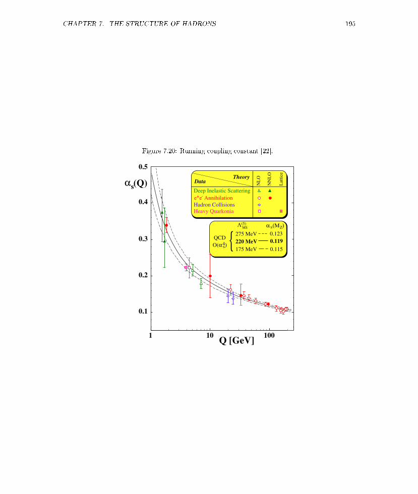
CHAPTER 7. THE STRUCTURE OF HADRONS 195
Figure 7.20: Running coupling constant [22].
QCD
O(α )
275 MeV
175 MeV
Λ MS(5)
α (Μ )s Z
0.123
0.115
0.1
0.2
0.3
0.4
0.5
αs (Q)
1 10 100Q [GeV]
Heavy Quarkonia
Hadron Collisions
e+e- Annihilation
Deep Inelastic Scattering
NL
O
NN
LO
TheoryData
Lat
tice
220 MeV 0.119s4

CHAPTER 7. THE STRUCTURE OF HADRONS 196
We see that when 11− 23nf > 0, αs(µ) < αs(µ0) for µ > µ0. We can make expansion of the inverse
of ln µ2
µ20, we get the leading term,
αs(Q2) =
4π
(11− 2nf/3) ln(Q2/Λ2)(7.153)
where Λ is an arbitray energy scale. One observes that the essential dierence of αS(Q2) fromαQED(Q2) is that αS(Q2) decreases as Q2 increases, just opposite to αQED(Q2). This is called theasymptotic freedom. The physics is shown in Fig. 7.19. The quark-antiquark vacuum polarizationscreen the color charge in a similar way as in QED. But there is another process which cannotbe found in QED: a color charge can turn into another color charge by radiating a gluon carryingaway the original charge. The contribution of this process dominate over the QED-like one provided11 > 2nf/3 which is true for nf = 6 in the real world. The data and theoretical predictions forαs(Q
2) are shown in Fig. 7.20.The running coupling constant can be very large at the infrared end which means stong couplings.
This indicates a very important eect, color connement, where quarks and gluons can not be seenfreely at low energies. We will explain the color connement in the next section.
7.2.4 Phenomenological illustration of the connement [7]
Consider a system of quarks and gluons in a volume of L3, the coupling constant at length scale l isgiven by gl, one can prove gL > gl for L > l. Let's introduce a color dielectric constant in vacuumκL and a renormalized coupling constant g ≡ gl where l is the length in the order of proton radius.Then κL is dened by
g2L =
g2
κL(7.154)
So when L = l, we have κl = 1 and
κL < κl, for L > l (7.155)
The perturbation theory gives to the leading order,
κLκl
=1
1 + αs2π
(11− 2
3nf)
lnLl(7.156)
When L → ∞, we have κ∞ = 0 and g2∞ → ∞. So the vacuum is a medium with extremely strong
couplings.In electromagnetism, the dielectric constant is κvacuum = 1. One can prove that κ ≥ 1 for all
physical dielectric media. This can be seen by the electric displacement vector,
D = E + 4πP = κE (7.157)
where the polarization vector P is parallel to E, so one has κ ≥ 1.There is an electromagnetism analogy to the color connement. We consider a hypothetical
medium with a small dielectric constant,
κ ≡ κm 1 or = 0 (7.158)
i.e. the medium is anti-screening because the polarization vector is anti-parallel to the electric eld.If we put a test charge into the medium, a hole must be formed as shown in Fig. 7.21. Inside thehole is the perturbative vacuum with κ = 1. We can estimate the radius of this hole. Assume Eout,Dout ,Ein and Din are normal components of the elds outside and inside the sphere. We have
Din = Ein = Dout =e
R2
Eout =e
κmR2(7.159)

CHAPTER 7. THE STRUCTURE OF HADRONS 197
Figure 7.21: The eect of a test charge in an anti-screening medium.
+
+
+
+
+ +
++
kappa=1
anti−chargecharge
kappa=1
kappa=1
charge−qa
charge−qbcharge−qc
meson
baryon
kappa<<1
where e is the total electric charge of a charge distribution and R is the radius of the hole. Theelectric energies in the medium and vacuum are given by
Umout =1
8π
∫ ∞R
dΩdrr2D ·E =1
2
e2
κmR
Uvacout =1
2
e2
R(7.160)
where Uvacout So the energy dierence is
∆Ue =1
2
e2
R
(1
κm− 1
)(7.161)
One needs an energy Uhole to create a hole. It has two parts: the volume energy and the surface one,
Uhole ∼ C14π
3R3 + C24πR2 (7.162)
where C1 and C2 are two constants. The total energy is then
U = Umout + Uhole (7.163)
When κm → 0 and Uhole ∼ C14π3 R
3, i.e. dominated by the volume energy, we can nd the minimumof U as,
dU
dR=
d
dR
(1
2
e2
κmR+ C1
4π
3R3
)= −1
2
e2
κmR2+ C14πR2 = 0 (7.164)

CHAPTER 7. THE STRUCTURE OF HADRONS 198
Figure 7.22: The splitting of a bag.
Table 7.10: Comparison with superconductivity.
superconductivity (QED) hadron (QCD)H Ea
µin = 0 κvac = 0µvac = 1 κin = 1internal externalexternal internal
which gives
Rmin =
(e2
8πκmC1
)1/4
Umin =1
2
e2
κmRmin+ C1
4π
3R3min
∼ 4
3
(e2
2κm
)3/4
(4πC1)1/4 (7.165)
One can extend this example by introducing two test particles in opposite charges into the vacuum.Similar to the case of one test charge, a hole containing the two charges will form. This is the picturefor mesons with two opposite color charges. See Fig. 7.21.
When the couplings are extermely strong, there exists a strong repulsive force exerting on thecolor charges. This is analogous to Van der Waals force between two helium atoms. There is also ananalogy between the Meissner eect in a superconductor and the color connement. See Table 7.10and Fig. 7.23.
Exercise 62. Determine Rmin and Umin when Uhole ∼ C24πR2, i.e. the hole energy is onlyfrom the surface.

CHAPTER 7. THE STRUCTURE OF HADRONS 199
Figure 7.23: Comparison of superconductivity and hadron.
mu=0 anti−chargecharge
kappa=1
kappa−vacuum
mu−vacuum

Chapter 8
Acknowledgement
The author thanks following students who took this course and pointed out several errors in thislecture note: Dai Lei (2008-09 fall semester), Wu Ying-hai (2008-09 fall semester), Chen Peng-fei(2009-10 fall semester), Liu Pei-fan (2014 spring semester).
200

Appendix A
Nucleon-nucleon scattering theory
A.1 Nucleon-nucleon scatterings
The nucleon-nucleon interaction is a basic for understanding the nuclear force, for a review of thistopic, see, e.g., Ref. [29]. The scattering experiments is one of the most ecient tools to detect theproperties of particles. They are widely used in nuclear and particle physics. One of the earliestattempt was made in the Rutherford's experiment where the alpha-particles were used to bombardthe atoms. It shows that there is a nucleus inside the atom. In 1960s, in order to nd the structure ofnucleons Hofstadter used high energy electron-nucleon scatterings, which uncovers that the nucleonis not a point-like particle but has a nite size.
A.2 The stationary scattering wave function
Let us consider the non-relativistic scattering of a spinless particle of mass m by a central potentialV (r). The time-dependent Schroedinger equation is[
− 1
2m∇2 + V (r)
]ψ(t, r) = i
∂ψ(t, r)
∂t(A.1)
For stationary solution,
ψ(t, r) = e−iEtψ(r) (A.2)
where E = k2/2m. So the time-independent Schroedinger equation becomes[∇2 + k2 − 2mV (r)
]ψ(r) = 0 (A.3)
We assume that the potential V (r) tends to zero faster than 1/r as r goes to innity. The asymptotic
form of the wave function at r →∞ is denoted by ψ(+)k (r),
ψ(+)k (r) → A
[eik·r + f(θ, φ)
eikr
r
](A.4)
where the rst term of Eq. (A.4) is the incident wave along k, while the second term is the scatteringwave. We can choose the incident momentum k = kz along the z-axis, so f(θ, φ) = f(θ) dependingonly on the polar angle. This is because the incident wave has rotational symmetry which is conservedduring the scattering by a central potential.
201

APPENDIX A. NUCLEON-NUCLEON SCATTERING THEORY 202
Figure A.1: Scattering of a plane wave.
O
theta
phi
cross−section−area
incident−momentum
A.3 Cross section
The cross section σ(Ω)dΩ = dσdΩdΩ is the number of particles emitted per unit time and unit incident
ux within the solid angle dΩ about the direction Ω(θ, φ). One can obtain it by computing theoutgoing ux of particles scattered through the spherical surface r2dΩ devided by the incident ux.
The probability current density is
j(r) = −i 1
2m[ψ∗∇ψ − (∇ψ∗)ψ] =
1
mIm(ψ∗∇ψ) (A.5)
It satises the continuity equation,
∇ · j +∂ρ
∂t= 0 (A.6)
where ρ = |ψ|2 is the probability density. Since ∂ρ∂t = 0 in the stationary case, one has
∇ · j = 0 (A.7)
Now we try to calculate the current density. In spherical coordinates, we have
∇ = r∂
∂r+ θ
1
r
∂
∂θ+ φ
1
r sin θ
∂
∂φ(A.8)
The radial outgoing ux is
j · r =1
mIm
AA∗
[e−ikz + f∗(θ)
e−ikr
r
]∂
∂r
[eikz + f(θ)
eikr
r
]=
1
m|A|2Im
[e−ikz
∂
∂reikz
]+
1
m|A|2|f(θ)|2Im
[e−ikr
r
∂
∂r
eikr
r
]+
1
m|A|2Im
[f(θ)e−ikz
∂
∂r
eikr
r+ f∗(θ)
e−ikr
r
∂
∂reikz
]= (jinc + jout + jint) · r (A.9)
Here the ux corresponding to the incident wave
ψkz(r) = Aeikz (A.10)
is given by
jinc =1
mz|A|2Im
[e−ikz
∂
∂zeikz
]= z|A|2 k
m= z|A|2v (A.11)

APPENDIX A. NUCLEON-NUCLEON SCATTERING THEORY 203
One can verify
jinc · r =1
m|A|2Im
[e−ikz
∂
∂reikz
]= |A|2 1
mk cos θ (A.12)
The outgoing ux is
jout · r =1
m|A|2|f(θ)|2Im
[e−ikr
r
∂
∂r
eikr
r
]≈ |A|2 |f(θ)|2
r2
k
m+O(1/r3) (A.13)
The inteference term is given by
jint · r =1
m|A|2Im
[f(θ)e−ikz
∂
∂r
eikr
r+ f∗(θ)
e−ikr
r
∂
∂reikz
]= |A|2 k
m
1
rRe[f(θ)eik(r−z) + f∗(θ) cos θe−ik(r−z)
]+O(1/r2) (A.14)
We see that as r → ∞, the exponential factor e±ik(r−z) oscillates drastically except at the forwarddirection at θ = 0. The interference term can be neglected except at forward direction.
The particle outgoing ux through the spherical area r2dΩ is
|A|2 |f(θ)|2r2
k
mr2dΩ = |A|2 k
m|f(θ)|2dΩ (A.15)
Dividing by the incident ux |A|2v, one gets the dierential cross section,dσ
dΩ= |f(θ, φ)|2 (A.16)
The total cross section is then
σ =
∫dΩ
dσ
dΩ=
∫dΩ|f(θ, φ)|2 (A.17)
A.4 The optical theorem
Now consider the forward scattering at θ = 0. Let us compute the ux at forward direction from Eq.(A.14),∫
θ=0
dΩr2jint · r ≈∫θ=0
dΩr2|A|2 km
1
rRe[f(θ = 0)eikr(1−cos θ) + f∗(θ = 0)e−ikr(1−cos θ)
]= r|A|2 k
m4π
∫ 1
cos δθ
d cos θRe[f(θ = 0)eikr(1−cos θ)
]≈ r|A|2 k
m4πRe
[i
krf(θ = 0)(1− eikr(1−cos δθ))
]≈ r|A|2 k
m4πRe
[i
krf(θ = 0)(1− eikrδθ2/2)
]≈ −|A|2 1
m4πImf(θ = 0) (A.18)
We have used the fact that krδθ2/2 → ∞ when r → ∞, so the phase factor eikrδθ2/2 drastically
uctuates and is negligible. We see in Eq. (A.18) that the total ux from jint · r is negative whichmeans it goes inside the sphere. In contrast the total ux from incident wave is zero,∫
dΩjinc · r = 0 (A.19)

APPENDIX A. NUCLEON-NUCLEON SCATTERING THEORY 204
which is easy to understand: the incident wave goes inside the region at θ = π and leaves the regionat θ = 0.
From the continuity equation ∇ · j = 0, we have
r2
∫dΩj · r = 0 (A.20)
which reads
r2
∫dΩ(jout + jint) · r = 0 (A.21)
and can be written as
|A|2 1
m
[k
∫dΩ|f(Ω)|2 − 4πImf(θ = 0)
]= 0 (A.22)
So the total cross section is related to the imaginary part of the scattering amplitude in the forwarddirection,
σtot =4π
kImf(θ = 0) (A.23)
This is called the optical theorem, a result of probability conservation, which states that the totalcross section is given by the imaginary part of the forward scattering amplitude. This proof is basedon the elastic scattering.
A.5 Partial wave method
We consider a central potential V (r). In spherical coordinates, the Hamiltonian H = −(1/2m)∇2 +Vreads,
H = − 1
2m
[1
r2
∂
∂r
(r2 ∂
∂r
)+
1
r2 sin θ
∂
∂θ
(sin θ
∂
∂θ
)+
1
r2 sin2 θ
∂2
∂φ2
]+ V (r)
= − 1
2m
[1
r2
∂
∂r
(r2 ∂
∂r
)− L2
r2
]+ V (r) (A.24)
with L2 given by
L2 = −[
1
sin θ
∂
∂θ
(sin θ
∂
∂θ
)+
1
sin2 θ
∂2
∂φ2
](A.25)
One can verify
[H,L2] = [H,Lz] = 0 (A.26)
Because the operators H,L2, Lz all commute to each other, the state can be labeled by quantumnumbers n, l,m, where n labels the energy level, l the angular momentum, m the projection to the
third axis. The scattering wave function ψ(+)k can be expanded in partial waves as
ψ(+)k (k, r) =
∞∑l=0
+l∑m=−l
clm(k)Rlm(k, r)Ylm(θ, φ) (A.27)
If there is no dependence on the magnetic quantum number m, so Rlm(k, r) is written as Rl(k, r).We obtain [
d2
dr2+
2
r
d
dr+ k2 − l(l + 1)
r2− U(r)
]Rl(k, r) = 0 (A.28)

APPENDIX A. NUCLEON-NUCLEON SCATTERING THEORY 205
It is convenient to use
Rl(k, r) =ul(k, r)
r(A.29)
to rewrite Eq. (A.28) as [d2
dr2+ k2 − l(l + 1)
r2− U(r)
]ul(k, r) = 0 (A.30)
For V (r) = 0, we can also use variable ρ = kr to rewrite Eq. (A.28) as[d2
dρ2+
2
ρ
d
dρ+ 1− l(l + 1)
ρ2
]Rl(ρ) = 0 (A.31)
whose solution is the spherical Bessel function.For free particles with V (r) = 0, the solutions to Eq. (A.31) are spherical Bessel functions
Rl(kr) = C(1)l (k)jl(kr) + C
(2)l (k)nl(kr) (A.32)
orRl(kr) = D
(1)l (k)h
(1)l (kr) +D
(2)l (k)h
(2)l (kr) (A.33)
At r → 0 only jl(kr) is nite and all others diverge. At r →∞, we have
Rl(k, r) → C(1)l (k)
1
krsin
(kr − l
2π
)− C(2)
l (k)1
krcos
(kr − l
2π
)∼ 1
kr
√[C
(1)l (k)]2 + [C
(2)l (k)]2
×
C(1)l (k) sin
(kr − l
2π)√
[C(1)l (k)]2 + [C
(2)l (k)]2
− C(2)l (k) cos
(kr − l
2π)√
[C(1)l (k)]2 + [C
(2)l (k)]2
∼ 1
krAl(k) sin
[kr − l
2π + δl(k)
](A.34)
where we have used
Al(k) =
√[C
(1)l (k)]2 + [C
(2)l (k)]2
tan δl(k) = −C(2)l (k)
C(1)l (k)
(A.35)
and δl(k) is called the phase shift. The usual normalizations of scattering wave functions at r → ∞are Al(k) = 1 or Al(k) = 1/ cos δl.
A.5.1 Scattering amplitude and cross section
The scattering wave function at r →∞ is
ψ(+)k (r) → A
[eikz + f(θ)
eikr
r
](A.36)
where the rst term is the incident wave and the second term is the scattering wave. It is easyto verify that both terms are eigen wave function of the Schroedinger equation at r → ∞ wherel(l + 1)/r2 → 0 and V (r)→ 0. We can expand the plane wave eikz as
eikz =
∞∑l=0
(2l + 1)iljl(kr)Pl(cos θ) (A.37)

APPENDIX A. NUCLEON-NUCLEON SCATTERING THEORY 206
The proof can be found in the Appendix. Then the scattering wave function can be written as
ψ(+)k (r) ∼
∞∑l=0
(2l + 1)iljl(kr)Pl(cos θ) + f(θ)eikr
r
∼∞∑l=0
(2l + 1)il1
krsin
(kr − l
2π
)Pl(cos θ) + f(θ)
eikr
r
∼∞∑l=0
(2l + 1)il1
2ikr
exp
[i
(kr − l
2π
)]− exp
[−i(kr − l
2π
)]Pl(cos θ)
+f(θ)eikr
r(A.38)
If we assume for real δl(k),
f(θ) =
∞∑l=0
(2l + 1)flPl(cos θ)
=1
2ik
∞∑l=0
(2l + 1) exp[2iδl(k)]− 1Pl(cos θ)
=1
2ik
∞∑l=0
(2l + 1) exp[2iδl(k)]− 1Pl(cos θ)
=1
k
∞∑l=0
(2l + 1) exp[iδl(k)] sin δl(k)Pl(cos θ) (A.39)
where the partial wave scattering amplitude is written as fl = (Sl − 1)/(2ik) where Sl = e2iδl(k). Wethen obtain
ψ(+)k (r) ∼
∞∑l=0
(2l + 1)il1
2ikrPl(cos θ)
×
exp
[i
(kr − l
2π + 2δl(k)
)]− exp
[−i(kr − l
2π
)]∼
∞∑l=0
(2l + 1)il1
2ikrexp[iδl(k)]Pl(cos θ)
×
exp
[i
(kr − l
2π + δl(k)
)]− exp
[−i(kr − l
2π + δl(k)
)]∼
∞∑l=0
(2l + 1)il1
krexp[iδl(k)]Pl(cos θ) sin
(kr − l
2π + δl
)(A.40)
The dierential cross section is given by
dσ
dΩ= |f(θ)|2 =
1
k2
∞∑l,l′=0
(2l + 1)(2l′ + 1) exp[iδl(k)] exp[−iδl′(k)]
× sin δl(k) sin δl′(k)Pl(cos θ)Pl′(cos θ) (A.41)

APPENDIX A. NUCLEON-NUCLEON SCATTERING THEORY 207
Figure A.2: The positivity of the phase shift.
original−wave
phase−shift<0
phase−shift>0
The total cross section is then
σtot =
∫dΩ|f(θ, φ)|2
= 2π1
k2
∫ 1
−1
d(cos θ)
∞∑l,l′=0
(2l + 1)(2l′ + 1) exp[iδl(k)] exp[−iδl′(k)]
× sin δl(k) sin δl′(k)Pl(cos θ)Pl′(cos θ)
= 4π1
k2
∞∑l,l′=0
δll′(2l′ + 1) exp[iδl(k)] exp[−iδl′(k)] sin δl(k) sin δl′(k)
=4π
k2
∞∑l=0
(2l + 1) sin2 δl(k) (A.42)
where we have used ∫ 1
−1
dxPl(x)Pl′(x) =2
2l + 1δll′ (A.43)
The phase shift reect if the force is attractive or repulsive, one can see from ψ(+)k in Eq. (A.40)
δl =
> 0, attractive force< 0, repulsive force
(A.44)
See Fig. A.2 for illustration.We can estimate the maximum value of lmax as follows
lmax ∼ ka (A.45)
where a is the interaction range. For example, the range of nuclear force is about a few fm, for aparticle with the incident energy k ∼ 20 MeV/c,
ka ∼ 20× 1
197∼ 0.1 (A.46)
So the partial wave one has to take into account is s and p wave.
A.5.2 Inelastic scattering and total cross section
The wave function at r →∞ is given in Eq. (A.40), we rewrite it here,

APPENDIX A. NUCLEON-NUCLEON SCATTERING THEORY 208
ψ(r) ∼∞∑l=0
(2l + 1)1
2ikril Sl exp [i(kr − lπ/2)]− exp [−i(kr − lπ/2)]Pl(cos θ)
=
∞∑l=0
2l + 1
2ikr
[Sl exp(ikr) + (−1)l+1 exp(−ikr)
]Pl(cos θ) (A.47)
For elastic scatterings, δl is real and Sl is a purely phase factor, |Sl| = 1. For inelastic scatterings, δlis complex and |Sl| 6= 1. The probability current density is given in Eq. (A.5), its radial part is givenby
jr(r) =1
mIm(ψ∗∂rψ) =
1
mIm
∞∑l=0
i2l + 1
2kr
[S∗l exp(−ikr) + (−1)l+1 exp(ikr)
]Pl(cos θ)
×∞∑l′=0
2l′ + 1
2ikrik[Sl′ exp(ikr)− (−1)l
′+1 exp(−ikr)]Pl′(cos θ)
=1
m
1
4kr2Im
∞∑l,l′=0
i(2l + 1)(2l′ + 1)Pl(cos θ)Pl′(cos θ)
×[S∗l Sl′ − (−1)l+l
′ − (−1)l′+1S∗l exp(−2ikr) + (−1)l+1Sl′ exp(2ikr)
](A.48)
We can compute the outgoing ow,∫dΩjr(r)r
2 =π
2mkIm
∞∑l,l′=0
i(2l + 1)(2l′ + 1)2
2l + 1δll′
×[S∗l Sl − 1 + 2i(−1)l+1Im[Sl exp(2ikr)]
]=
π
mk
∞∑l=0
(2l + 1)(|Sl|2 − 1) (A.49)
When |Sl|2 = 1, no outgoing ow occurs, this corresponds to elastic scatterings. When |Sl|2 < 1,there is negative ow, this corresponds to an absorption. The dierential and total cross sections forinelastic scattering can be obtained by dividing the above by the incident ow k/m,
dσindΩ
=r2jr(r)
k/m
σin =
∫dΩjr(r)r
2
k/m=
π
k2
∞∑l=0
(2l + 1)(1− |Sl|2) (A.50)
The total elastic cross section is
σel =
∫dΩ|f |2 =
1
4k2
∞∑l,l′=0
(2l + 1)(2l′ + 1)(Sl − 1)(S∗l − 1)Pl(cos θ)Pl′(cos θ)
=π
k2
∞∑l=0
(2l + 1)|1− Sl|2 = 4π
∞∑l=0
(2l + 1)|fl|2 (A.51)
where the scattering amplitude f is given in by Eq. (A.39). The total cross section is then
σtot = σel + σin =2π
k2
∞∑l=0
(2l + 1)(1− ReSl) (A.52)
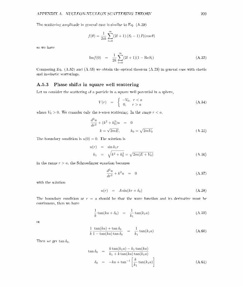
APPENDIX A. NUCLEON-NUCLEON SCATTERING THEORY 209
The scattering amplitude in general case is similar to Eq. (A.39)
f(θ) =1
2ik
∞∑l=0
(2l + 1) (Sl − 1)Pl(cos θ)
so we have
Imf(0) =1
2k
∞∑l=0
(2l + 1)(1− ReSl) (A.53)
Comparing Eq. (A.52) and (A.53) we obtain the optical theorem (A.23) in general case with elasticand in-elastic scatterings.
A.5.3 Phase shifts in square well scattering
Let us consider the scattering of a particle in a square well potential in a sphere,
V (r) =
−V0, r < a0, r > a
(A.54)
where V0 > 0. We consider only the s-wave scattering. In the range r < a,
d2u
dr2+ (k2 + k2
0)u = 0
k =√
2mE, k0 =√
2mV0 (A.55)
The boundary condition is u(0) = 0. The solution is
u(r) = sin k1r
k1 =√k2 + k2
0 =√
2m(E + V0) (A.56)
In the range r > a, the Schroedinger equation becomes
d2u
dr2+ k2u = 0 (A.57)
with the solution
u(r) = A sin(kr + δ0) (A.58)
The boundary condition at r = a should be that the wave function and its derivative must becontinuous, then we have
1
ktan(ka+ δ0) =
1
k1tan(k1a) (A.59)
or
1
k
tan(ka) + tan δ01− tan(ka) tan δ0
=1
k1tan(k1a) (A.60)
Then we get tan δ0,
tan δ0 =k tan(k1a)− k1 tan(ka)
k1 + k tan(ka) tan(k1a)
δ0 = −ka+ tan−1
[k
k1tan(k1a)
](A.61)

APPENDIX A. NUCLEON-NUCLEON SCATTERING THEORY 210
At ka 1, we can Taylor expand the above with respect to k, and obtain
k cot δ0 =1
a
k1a+ ka tan(ka) tan(k1a)
tan(k1a)− (k1a/ka) tan(ka)≈ − 1
as+
1
2reffk
2 (A.62)
We see that δ0 must be or the order k at the limit k → 0. Here the scattering length is
as = − limk→0
tan δ0(k)
k= a
[1− tan(k0a)
k0a
](A.63)
Note that as < 0 and δ0(k) > 0 for attractive interaction. For as < 0, k0a must be in [0, π/2]. Wehave used
1
a
k1a+ ka tan(ka) tan(k1a)
tan(k1a)− (k1a/ka) tan(ka)≈ − 1
as+
1
2reffk
2 (A.64)
where
reff = a− a3
3a2s
− 1
k20as
(A.65)
Because for s-wave and low energy, then the total cross section is
σtot = 4πsin2 δ0k2
=4π
k2 + k2 cot2 δ0=
4π
k2 + (−1/as + ρk2/2)2≈ 4πa2
[1− tan(k0a)
k0a
]2
+O(k2)
(A.66)When k0a = π/2,
δ0 = π/2 (A.67)
In this case the scattering length and cross section turn to negative innity. This corresponds to zeroenergy resonance. Note that k0a = π/2 is also the threshold for the appearance of one s-wave boundstate. When π/2 < k0a < π, there is one bound state, so the scattering length is positive. Whenk0a < π/2, there is no bound state, the scattering amplitude is negative.
A.5.4 Breit-Wigner formula
We conside the elastic scattering for simplicity. The total cross section is
σtot =4π
k2
∞∑l=0
(2l + 1) sin2 δl(E) (A.68)
When δl(E) satisfy
δl(E) ∼ (n+ 1/2)π, or sin2 δl(E) ∼ 1 (A.69)
the partial wave cross section reaches maximum and the resonant states occur. We can expand nearthe resonant energy E = E0 as
sin δl(E) ≈ sin δl(E0) +
[cos δl(E)
dδldE
]E0
(E − E0) ≈ 1
cos δl(E) ≈ cos δl(E0)−[sin δl(E)
dδldE
]E0
(E − E0)
= − dδldE
∣∣∣∣E0
(E − E0) = − 2
Γ(E − E0) (A.70)

APPENDIX A. NUCLEON-NUCLEON SCATTERING THEORY 211
Figure A.3: Argand plot for the partial wave amplitude. (a) ηl = 1; (b) ηl < 1.
resonant−energy
Imf_lImf_l
i/2 i/2
f_l
2delta_l
f_l
resonant−energy
Ref_l Ref_l
2delta_l
eta_leta
_l=1
where we have dened
Γ = 2/dδldE
∣∣∣∣E0
(A.71)
So the partial wave amplitude is
fl = exp[iδl(k)] sin δl(k)
=sin δl(k)
cos δl(k)− i sin δl(k)
≈ 1
− 2Γ (E − E0)− i =
−Γ/2
(E − E0) + iΓ/2
|fl|2 =Γ2/4
(E − E0)2 + Γ2/4(A.72)
If at E ∼ E0, the partial wave l is dominant, the cross section so we have
σtotl =4π
k2(2l + 1)
Γ2/4
(E − E0)2 + Γ2/4(A.73)
Generally the partial wave amplitude can be written as
fl =1
2i(ηle
2iδl − 1) =i
2− i
2ηle
2iδl (A.74)
The amplitude fl can be plotted on the Argand plot of Imfl versus Refl. The center of the circle isat (0, i/2). The resonant energy is located at (0, i(1 + ηl)/2) which corresponds to δl = π/2.
A.6 Scatterings of identical particles
There are two cases for scatterings of identical particles.(1) Two incident particles with spin-0. One cannot distinguish which particle is captured by the
detector. The dierential cross section is then
dσ
dΩ= |f(θ) + f(π − θ)|2 (A.75)

APPENDIX A. NUCLEON-NUCLEON SCATTERING THEORY 212
Figure A.4: Identicle scatterings.
θ
ba
θ
ba
a
b a
b
In the c.m.s frame, the dierential cross section is symmetric with respect to θ = π/2. In terms ofthe partial wave decomposition, the dierential cross section can be written
dσ
dΩ=
1
4k2
∣∣∣∣∣∞∑l=0
(2l + 1) exp[2iδl(k)]− 1 [Pl(cos θ) + Pl(− cos θ)]
∣∣∣∣∣2
=1
4k2
∣∣∣∣∣∞∑
l=even
(2l + 1) exp[2iδl(k)]− 1Pl(cos θ)
∣∣∣∣∣2
(A.76)
where we have used Eq. (A.39) and Pl(− cos θ) = (−1)lPl(cos θ).(2) Scatterings of two identical spin-1/2 particles. The wave function of two fermions are anti-
symmetric. The spin states are S = 0 and 1. For S = 0, the spatial wave function must be symmetric.For S = 1, the spatial wave function must be anti-symmetric. So we have
dσ
dΩ= |f(θ) + f(π − θ)|2, S = 0
dσ
dΩ= |f(θ)− f(π − θ)|2, S = 1 (A.77)
For the second line, the partial wave decomposition reads
dσ
dΩ=
1
4k2
∣∣∣∣∣∞∑
l=odd
(2l + 1) exp[2iδl(k)]− 1Pl(cos θ)
∣∣∣∣∣2
(A.78)
If the incident particles are not polarized, the probability in spin-0 state is 1/4, while that in spin-1state is 3/4. So the total dierential cross section is(
dσ
dΩ
)tot
=1
4
(dσ
dΩ
)S=0
+3
4
(dσ
dΩ
)S=1
(A.79)
A.7 Lippman-Schwinger equation and Green function method
We now introduce another method for scattering problems: Lippman-Schwinger or Green func-tion method. This method is suitable for high energy particle scatterings. The time-independentSchrödinger equation reads
(∇2 + k2)ψ(r) = U(r)ψ(r) (A.80)
where k2 = 2mE and U(r) = 2mV (r). The wave function satises the boundary condition at r →∞,Eq. (A.4). The solution ψ(r) is composed of a general solution of the homogeneous equation and a

APPENDIX A. NUCLEON-NUCLEON SCATTERING THEORY 213
Figure A.5: Scatterings of identical spin-1/2 particles.
θ
ba
θ
a b
θ
ba
θ
ba
special solution of the full equation,
ψ(r) = φk(r) +
∫d3r1G0(r− r1)U(r1)ψ(r1) (A.81)
where φk(r) is a general solution of(∇2 + k2)φk(r) = 0
The Green function G0(r− r′) satises
(∇2 + k2)G0(r− r1) = δ3(r− r1) (A.82)
Obviously one can verify that ψ(r) of the form in Eq. (A.81) obey the Schrödinger equation. Eqs.(A.81) can be written in a symbolic form
|ψ〉 = |φ〉+G0U |ψ〉
where |ψ〉 can be solved by
|ψ〉 = (1−G0U)−1 |φ〉 = (1 +GU) |φ〉 (A.83)
Note that G0 and U can thought of matrices in symbolic space. Here we have dened the full Greenfunction G,
G = (1−G0U)−1G0
The Green function G satises
[∇2 + k2 − U(r)]G(r− r1) = δ3(r− r1) (A.84)
So we can verify that |ψ〉 satises Eq. (A.80).

APPENDIX A. NUCLEON-NUCLEON SCATTERING THEORY 214
Figure A.6: The possible contours for the integral in Eq. (A.85).
x x
xx x x
x x−k−pole
contour2
contour3 contour4
contour1
−k−pole
−k−pole −k−pole
k−pole
k−polek−pole
k−pole
imagine−q imagine−q
real−qreal−q
real−q
imagine−q imagine−q
real−q
We can solve G0(r− r1) as
G0(r) = −∫
d3q
(2π)3eiq·r
1
q2 − k2= − 1
(2π)2
∫dqdθ sin θeiqr cos θ q2
q2 − k2
=i
(2π)2
1
r
∫ ∞0
dqq
q2 − k2
∫ 1
−1
d(iqr cos θ)eiqr cos θ
=i
(2π)2
1
r
∫ ∞0
dqq
q2 − k2(eiqr − e−iqr) =
i
(2π)2
1
r
∫ ∞−∞
dqqeiqr
q2 − k2
=i
2(2π)2
1
r
∫ ∞−∞
dqeiqr(
1
q − k +1
q + k
)(A.85)
We can extend q to compex plane and make it to the contour integral along C. To make the integralconverge, we assume Imq > 0 close the contour in the upper plane because eiqr → 0 in the upper halfcircle at r → ∞. There are four contours C1,2,3,4. The integrals of contour C1,2,3 give contributionsproportional to eikr+e−ikr, 0, and e−ikr respectively. For the outgoing wave we need the contributionproportional to eikr which comes only from C4. The choice of C4 can be implemented by making thereplacement 1
q2−k2 → 1q2−k2−iε . Eq. (A.85) can be carried out
G0(r) = − 1
4π
1
reikr (A.86)
If we treat the potential as perturbation, i.e. we take Born approximation, in the leading order

APPENDIX A. NUCLEON-NUCLEON SCATTERING THEORY 215
Eq. (A.81) or (A.83) becomes
ψ(r) ≈ φk(r)− 1
4π
∫d3r1
1
|r− r1|eik|r−r1|U(r1)φk(r1)
≈ φk(r)− 1
4π
∫d3r1
1
r − r1 cos θeik(r−r1 cos θ)U(r1)φk(r1)
≈ eik·r − 1
4πreikr
∫d3r1e
−i(kf−k)·r1U(r1) (A.87)
where kf = kr/r. The scattering amplitude is then
f(kf ,k) = − 1
4π
∫d3r1e
−i(kf−k)·r1U(r1) = − 1
4πU(kf − k) (A.88)

Appendix B
A: Bessel functions
The Bessel equation reads
d2y
dx2+
1
x
dy
dx+
(1− ν2
x2
)y = 0 (B.1)
where ν and x are any complex number. The solutions are the Bessel functions Jν(x) of the rstkind,
Jν(x) =
∞∑k=0
(−1)k1
k!
1
Γ(ν + k + 1)
(x2
)2k+ν
(B.2)
If ν is not an integer, then J−ν(x) is another independent solution. If Jν(x) = n an integer, then wehave
J−n(x) =
∞∑k=0
(−1)k1
k!
1
Γ(−n+ k + 1)
(x2
)2k−n
=
∞∑l=0
(−1)l+n1
(l + n)!
1
l!
(x2
)2l+n
= (−1)nJn(x) = Jn(−x) (B.3)
where we have used the fact that 1/(−l)! = 0 with l > 0. This means Jn(x) and J−n(x) are basicallythe same solution of the Bessel equation. Another independent solution is the Bessel function ofsecond kind. When x is real, Jn(x) is an oscillating function with a damping amplitude.
The generating function of Bessel functions is
ex(t−t−1)/2 =
∞∑n=−∞
Jn(x)tn, (0 < |t| <∞) (B.4)
One can write it in a dierent way by using t = ieϕ, x = kr,
eikr cos θ =
∞∑n=−∞
Jn(kr)ineinθ
= J0(kr) +
∞∑n=1
[Jn(kr)ineinθ + J−n(kr)i−ne−inθ
]= J0(kr) + 2
∞∑n=1
inJn(kr) cosnθ (B.5)
216

APPENDIX B. A: BESSEL FUNCTIONS 217
where we have used J−n(x) = (−1)nJn(x).The Bessel function of the second kind is dened by
Yν(x) =Jν(x) cos νπ − J−ν(x)
sin νπ(B.6)
If ν is not an integer, obviously Yν(x) is independent of Jν(x). One can prove that if ν = n, Yn(x) isalso an independent solution of Jn(x). Note that Yn(x) diverges at x = 0. For example, at x→ 0,
Y0(x) =2
πlnx
2
Yn(x) = − (n− 1)!
π
(x2
)−n(B.7)
Bessel functions of third kind H(1)ν (x) and H
(2)ν (x) are dened by
H(1)ν (x) = Jν(x) + iYν(x)
H(2)ν (x) = Jν(x)− iYν(x) (B.8)
The asymptotic forms of Bessel functions at |arg(x)| < π, |x| → ∞ are
Jν(x) =
√2
πxcos(x− νπ
2− π
4
)+O(x−3/2),
Yν(x) =
√2
πxsin(x− νπ
2− π
4
)+O(x−3/2),
H(1)ν (x) =
√2
πxexp
[i(x− νπ
2− π
4
)]+O(x−3/2),
H(2)ν (x) =
√2
πxexp
[−i(x− νπ
2− π
4
)]+O(x−3/2), (B.9)
The spherical Bessel functions are solutions of
d2y
dx2+
2
x
dy
dx+
[1− l(l + 1)
x2
]y = 0 (B.10)
Using y(x) = x−1/2η(x) and
dy
dx= −1
2
1
x√xη(x) +
1√x
dη(x)
dx
d2y
dx2=
3
4x−5/2η(x)− x−3/2η′(x) + x−1/2η′′(x)
d2y
dx2+
2
x
dy
dx=
3
4x−5/2η(x)− x−3/2η′(x) + x−1/2η′′(x)
+2
x
[−1
2
1
x√xη(x) +
1√x
dη(x)
dx
]= −1
4x−5/2η(x) + x−3/2η′(x) + x−1/2η′′(x) (B.11)
Then the spherical Bessel equation becomes the Bessel one
d2y
dx2+
2
x
dy
dx+
[1− l(l + 1)
x2
]y
= x−1/2
[d2η
dx2+
1
x
dη
dx+
(1− (l + 1/2)2
x2
)η
]= 0 (B.12)

APPENDIX B. A: BESSEL FUNCTIONS 218
whose solution is the Bessel function η ∼ Jl+1/2, Yl+1/2. The solutions y = x−1/2η(x) to the sphericalBessel equation are spherical Bessel functions
jl(x) =
√π
2xJl+1/2(x)
nl(x) =
√π
2xYl+1/2(x)
h(1)l =
√π
2xH
(1)l+1/2(x) = jl(x) + inl(x)
h(2)l =
√π
2xH
(2)l+1/2(x) = jl(x)− inl(x) (B.13)
They satisfy
ψl−1 + ψl+1 =2l + 1
xψl
lψl−1 − (l + 1)ψl+1 = (2l + 1)ψ′l (B.14)
where ψl stands for jl(x), nl(x), h(1)l or h
(2)l .
We can expand the plane wave eikz in terms of Legendre polynomials
eikr cos θ =
∞∑l=0
cl(kr)Pl(cos θ)
where
cl(kr) =2l + 1
2
∫ 1
−1
dxeikrxPl(x)
=2l + 1
2l+1
1
l!
∫ 1
−1
dxeikrxdl
dxl(x2 − 1)l
=2l + 1
2l+1
1
l!(−ikr)
∫ 1
−1
dxeikrxdl−1
dxl−1(x2 − 1)l
=2l + 1
2l+1
1
l!(−ikr)l
∫ 1
−1
dxeikrx(x2 − 1)l
=2l + 1
2l+1
1
l!(−ikr)l
∞∑m=0
(ikr)m
m!
∫ 1
−1
dxxm(x2 − 1)l
=2l + 1
2l+1
1
l!(−ikr)l2
∞∑s=0
(ikr)2s
(2s)!
∫ 1
0
dxx2s(x2 − 1)l (B.15)
where we have used
dl−n
dxl−n(x2 − 1)l
∣∣∣∣1−1
= 0 (B.16)
where n = 1, 2, ..., l − 1. The integral is evaluated as∫ 1
−1
dxx2s(x2 − 1)l = (−1)l1
2
∫ 1
0
duus−1/2(1− u)l
= (−1)l1
2
Γ(s+ 1/2)F (l + 1)
Γ(l + s+ 3/2)
=(−1)ll!(2s)!
√π
22s+1s!Γ(l + s+ 3/2)(B.17)

APPENDIX B. A: BESSEL FUNCTIONS 219
where we have used
Γ(s+ 1/2) = Γ(2s+ 1)2−2s√π/Γ(s+ 1) =
(2s)!√π
22ss!(B.18)
Eq. (B.15) becomes
cl(kr) =2l + 1
2il(kr/2)l
∞∑s=0
(−1)s(kr/2)2s
√π
s!Γ(l + s+ 3/2)
= (2l + 1)il√
π
2kr
∞∑s=0
(−1)s(kr/2)2s+l+1/2 1
s!Γ(l + s+ 3/2)
= (2l + 1)il√
π
2krJl+1/2(kr) = (2l + 1)iljl(kr) (B.19)

Appendix C
B: Spherical harmonic functions
A few lowest order harmonic functions. The Legendre and associated Legendre polynomials are givenby
Pl(x) =1
2ll!
dl
dxl(x2 − 1)l
Pml (x) = (1− x2)m/2dm
dxmPl(x)
=(1− x2)m/2
2ll!
dl+m
dxl+m(x2 − 1)l
Note that for the associated Legendre functions, the rst equality holds for l ≥ m ≥ 0, but the secondone holds for all |m| ≤ l. They satisfy
Pl(−x) = (−1)lPl(x)∫ 1
−1
dxPl(x)Pk(x) =2
2l + 1δlk∫ 1
−1
dxPml (x)Pmk (x) =(l +m)!
(l −m)!
2
2l + 1δlk
A few lowest order terms are
P0(x) = 1, P1(x) = x, P2(x) =1
2(3x2 − 1),
P3(x) =1
2(5x3 − 3x), P4(x) =
1
8(35x4 − 30x2 + 3)
P5(x) =1
8(63x5 − 70x3 + 15x),
P6(x) =1
16(231x6 − 315x4 + 105x2 − 5)
The spherical harmonic functions are dened
Ylm = (−1)m√
2l + 1
4π
√(l −m)!
(l +m)!Pml (cos θ)eimϕ, |m| ≤ l
Y ∗lm = (−1)mYl,−m
For m 6= 0, we have
Yl,0 =
√2l + 1
4πPl(cos θ)
220

APPENDIX C. B: SPHERICAL HARMONIC FUNCTIONS 221
The orthogonal and complete property,∫dΩY ∗lmYl′m′ = δll′δmm′
A few lowest order functions
Y00 =
√1
4π
Y10 =
√3
4πcos θ, Y1,±1 = ∓
√3
8πsin θe±iϕ
Y20 =1
2
√5
4π(3 cos2 θ − 1), Y2,±1 = ∓
√15
8πsin θ cos θe±iϕ,
Y2,±2 =1
2
√15
8πsin2 θe±2iϕ
Vector spherical harmonic functions are
YLlM (θ, φ) =∑m,n
CLMlm,1nYlm(θ, φ)en (C.1)
The gradient formula
∇[f(r)Ylm(θ, φ)] = Ylm∇f(r) + f(r)∇Ylm= f ′(r)rYlm + eθf(r)
1
r
∂Ylm∂θ
+ eφf(r)1
r sin θ
∂Ylm∂φ
where we have used
∇ = er∂
∂r+ eθ
∂
r∂θ+ eφ
∂
r sin θ∂φ
∂Ylm∂θ
= (−1)m+1 1
sin θ
√2l + 1
4π
√(l −m)!
(l +m)!sin2 θ
d
d cos θPml (cos θ)eimφ
= (−1)m+1 1
sin θ
√2l + 1
4π
√(l −m)!
(l +m)!
×[
(l + 1)(l +m)
2l + 1Pml−1(cos θ)− l(l −m+ 1)
2l + 1Pml+1(cos θ)
]eimφ
= − 1
sin θ(l + 1)
√(l −m)(l +m)
(2l − 1)(2l + 1)Yl−1,m +
1
sin θl
√(l −m+ 1)(l +m+ 1)
(2l + 1)(2l + 3)Yl+1,m
=1
sin θ(−c1Yl−1,m + c2Yl+1,m)
∂Ylm∂φ
= imYlm
eθ = ex cos θ cosφ+ ey cos θ sinφ− ez sin θ
= −e11√2
cos θe−iφ + e−11√2
cos θeiφ − ez sin θ
eφ = −ex sin θ + ey cos θ
=1√2
(sin θ + i cos θ)e1 +1√2
(− sin θ + i cos θ)e−1
ex =1√2
(−e1 + e−1)
ey =i√2
(e1 + e−1)

APPENDIX C. B: SPHERICAL HARMONIC FUNCTIONS 222
We obtain
eθf(r)1
r
∂Ylm∂θ
+ eφf(r)1
r sin θ
∂Ylm∂φ
=f(r)
r sin θ(−c1Yl−1,m + c2Yl+1,m)(
−e11√2
cos θe−iφ + e−11√2
cos θeiφ − ez sin θ
)+f(r)
r sin θimYlm
[1√2
(sin θ + i cos θ)e1 +1√2
(− sin θ + i cos θ)e−1
]

Appendix D
Solutions to problems
Exercises in (6.3.2). We use S12 = T ijσ1iσ2j = 2T ijSiSj where Tij = 3rirj−δij and Si = 1
2 (σ1i+σ2i).We can express the total spin operators in terms of ladder operators S± = S1 ± iS2 with
S±χ1,m =√
(1∓m)(1±m+ 1)χ1,m±1
S±χ1,1 = 0,√
2χ1,0
S±χ1,0 =√
2χ1,±1
S±χ1,−1 =√
2χ1,0, 0
with
S1 =1
2(S+ + S−)
S2 =1
2i(S+ − S−)
S21 =
1
4(S2
+ + S2− + S+S− + S−S+)
S1S2 = − i4
(S2+ − S2
− − S+S− + S−S+)
S22 = −1
4(S2
+ + S2− − S+S− − S−S+)
S2S1 = − i4
(S2+ − S2
− + S+S− − S−S+)
We get
SiSjχ1,1 =
12 (χ1,−1 + χ1,1) i
2 (χ1,−1 + χ1,1)√
22 χ1,0
i2 (χ1,−1 − χ1,1) 1
2 (−χ1,−1 + χ1,1)√
22 iχ1,0
0 0 χ1,1
SiSjχ1,0 =
χ1,0 0 00 χ1,0 0√
22 (χ1,1 − χ1,−1) −
√2
2 i(χ1,1 + χ1,−1) 0
SiSjχ1,−1 =
12 (χ1,1 + χ1,−1) − i
2 (χ1,1 + χ1,−1) −√
22 χ1,0
− i2 (χ1,1 − χ1,−1) − 1
2 (χ1,1 − χ1,−1) i√
22 χ1,0
0 0 χ1,−1
223

APPENDIX D. SOLUTIONS TO PROBLEMS 224
where we have used for χ1,1,
S1S1χ1,1 =1
4(S2− + S+S−)χ1,1 =
1
2(χ1,−1 + χ1,1)
S1S2χ1,1 =i
4(S2− + S+S−)χ1,1 =
i
2(χ1,−1 + χ1,1)
S1S3χ1,1 = S1χ1,1 =1
2(S+ + S−)χ1,1 =
√2
2χ1,0
S2S1χ1,1 =i
4(S2− − S+S−)χ1,1 =
i
2(χ1,−1 − χ1,1)
S2S2χ1,1 = −1
4(S2− − S+S−)χ1,1 =
1
2(−χ1,−1 + χ1,1)
S2S3χ1,1 = − 1
2iS−χ1,1 =
√2
2iχ1,0
S3S1χ1,1 =1
2S3(S+ + S−)χ1,1 =
1
2S3(S+ + S−)χ1,1 = 0
S3S2χ1,1 =1
2iS3(S+ − S−)χ1,1 = 0
S3S3χ1,1 = χ1,1
and for χ1,0,
S1S1χ1,0 =1
4(S+S− + S−S+)χ1,0 = χ1,0
S1S2χ1,0 = − i4
(−S+S− + S−S+)χ1,0 = 0
S1S3χ1,0 = 0
S2S1χ1,0 = − i4
(S+S− − S−S+)χ1,0 = 0
S2S2χ1,0 = −1
4(−S+S− − S−S+)χ1,0 = χ1,0
S2S3χ1,0 = 0
S3S1χ1,0 =1
2S3(S+ + S−)χ1,0 =
√2
2(χ1,1 − χ1,−1)
S3S2χ1,0 =1
2iS3(S+ − S−)χ1,0 = −
√2
2i(χ1,1 + χ1,−1)
S3S3χ1,0 = 0

APPENDIX D. SOLUTIONS TO PROBLEMS 225
and for χ1,−1,
S1S1χ1,−1 =1
4(S2
+ + S−S+)χ1,−1 =1
2(χ1,1 + χ1,−1)
S1S2χ1,−1 = − i4
(S2+ + S−S+)χ1,−1 = − i
2(χ1,1 + χ1,−1)
S1S3χ1,−1 = −1
2(S+ + S−)χ1,−1 = −
√2
2χ1,0
S2S1χ1,−1 = − i4
(S2+ − S−S+)χ1,−1 = − i
2(χ1,1 − χ1,−1)
S2S2χ1,−1 = −1
4(S2
+ − S−S+)χ1,−1 = −1
2(χ1,1 − χ1,−1)
S2S3χ1,−1 = i1
2(S+ − S−)χ1,−1 = i
√2
2χ1,0
S3S1χ1,−1 =1
2S3(S+ + S−)χ1,−1 = 0
S3S2χ1,−1 =1
2iS3(S+ − S−)χ1,−1 = 0
S3S3χ1,−1 = χ1,−1
Then we obtain
S12φ11S = 2
1√4πT ijSiSjχ1,1
= 21√4π
[T 11 1
2(χ1,−1 + χ1,1) + T 12 i
2(χ1,−1 + χ1,1) + T 13
√2
2χ1,0
+T 21 i
2(χ1,−1 − χ1,1) + T 22 1
2(−χ1,−1 + χ1,1) + T 23
√2
2iχ1,0 + T 33χ1,1
]
=1√4π
[(T 11 − T 22 + i2T 12
)χ1,−1 +
√2(T 13 + iT 23)χ1,0 + T 33χ1,1
]=√
8φ11D
S12φ10S = 2
1√4πT ijSiSjχ1,0
= 21√4π
[T 11χ1,0 + T 22χ1,0 + T 31
√2
2(χ1,1 − χ1,−1)− T 32
√2
2i(χ1,1 + χ1,−1)
]
=1√4π
[2(T 11 + T 22
)χ1,0 +
√2(T 13 − iT 23)χ1,1 −
√2(T 13 + iT 23)χ1,−1
]=√
8φ10D

APPENDIX D. SOLUTIONS TO PROBLEMS 226
S12φ1,−1S = 2
1√4πT ijSiSjχ1,−1
= 21√4π
[T 11 1
2(χ1,1 + χ1,−1)− iT 12χ1,1 − T 13
√2
2χ1,0
−T 22 1
2(χ1,1 − χ1,−1) + iT 23
√2
2χ1,0 + T 33χ1,−1
]
=1√4π
[(T 11 − T 22 − i2T 12
)χ1,1 +
√2(−T 13 + iT 23)χ1,0 + T 33χ1,−1
]=√
8φ1,−1D
where φ1mD are given by
φ11D =
∑m1,m2
c(1;m1,m2)Y2m1(θ, ϕ)χ1m2
=
√3
5Y2,2(θ, ϕ)χ1,−1 −
√3
10Y2,1(θ, ϕ)χ1,0 +
√1
10Y2,0(θ, ϕ)χ1,1
=
√3
5
1
4
√15
2π
1
3
(T 11 − T 22 + i2T 12
)χ1,−1 +
√3
10
√15
8π
1
3
(T 13 + iT 23
)χ1,0 +
√1
10
1
2
√5
4πT 33χ1,1
=1
4
1√2π
(T 11 − T 22 + i2T 12
)χ1,−1 +
1
4
1√π
(T 13 + iT 23
)χ1,0 +
1
4
1√2πT 33χ1,1
=1√4π
1√8
[(T 11 − T 22 + i2T 12
)χ1,−1 +
√2(T 13 + iT 23)χ1,0 + T 33χ1,1
]
φ10D =
∑m1,m2
c(0;m1,m2)Y2m1(θ, ϕ)χ1m2
=
√3
10Y2,1(θ, ϕ)χ1,−1 −
√2
5Y2,0(θ, ϕ)χ1,0 +
√3
10Y2,−1(θ, ϕ)χ1,1
= −√
3
10
√15
8π
1
3
(T 13 + iT 23
)χ1,−1 −
√2
5
1
2
√5
4πT 33χ1,0 +
√3
10
√15
8π
1
3
(T 13 − iT 23
)χ1,1
= − 1
4√π
(T 13 + iT 23
)χ1,−1 −
√2
2√πT 33χ1,0 +
1
4√π
(T 13 − iT 23
)χ1,1
=1√4π
1√8
[−√
2(T 13 + iT 23
)χ1,−1 − 4T 33χ1,0 +
√2(T 13 − iT 23
)χ1,1
]
φ1,−1D =
∑m1,m2
c(−1;m1,m2)Y2m1(θ, ϕ)χ1m2
=
√3
5Y2,−2(θ, ϕ)χ1,1 −
√3
10Y2,−1(θ, ϕ)χ1,0 +
√1
10Y2,0(θ, ϕ)χ1,−1
=
√3
5
1
4
√15
2π
1
3
(T 11 − T 22 − i2T 12
)χ1,−1 −
√3
10
√15
8π
1
3
(T 13 − iT 23
)χ1,0 +
√1
10
1
2
√5
4πT 33χ1,−1
=1
4
1√2π
(T 11 − T 22 − i2T 12
)χ1,−1 −
1
4
1√π
(T 13 − iT 23
)χ1,0 +
1
4
1√2πT 33χ1,1
=1√4π
1√8
[(T 11 − T 22 − i2T 12
)χ1,−1 −
√2(T 13 − iT 23)χ1,0 + T 33χ1,1
]

APPENDIX D. SOLUTIONS TO PROBLEMS 227
Now we have proved S12φ1mS =
√8φ1m
D . By acting S12 on it again and use
S212 = [3(r · σ1)(r · σ2)− (σ1 · σ2)][3(r · σ1)(r · σ2)− (σ1 · σ2)]
= 9 + (σ1 · σ2)2 − 3(r · σ1)σ1i(r · σ2)σ2i − 3σ1i(r · σ1)σ2i(r · σ2)
= 9 + (σ1 · σ2)2 − 3rarc(δia − iεiabσ1b)(δic − iεicdσ2d)− 3rarc(δia + iεiabσ1b)(δic + iεicdσ2d)
= 3 + (σ1 · σ2)2 + 3rarcεiabεicdσ1bσ2d + 3rarcεiabεicdσ1bσ2d
= 3 + (σ1 · σ2)2 + 6rarc(δacδbd − δadδbc)σ1bσ2d
= 3 + (σ1 · σ2)2 + 6(δbd − rbrd)σ1bσ2d
= 3 + (σ1 · σ2)2 − 4(σ1 · σ2)− 2S12
= (σ1 · σ2 + 2)2 − 1− 2S12
we get
S212φ
1mS =
√8S12φ
1mD = 8φ1m
S − 2S12φ1mS
S12φ1mD =
√8φ1m
S − 2φ1mD
Exercises in (3.6).In order to change the life of the energy level in second into the energy width in eV, we use the
relation in the natural unit, c = 3× 10²³ fm/s = 1, which gives 1 s = 3× 10²³ fm. So the width is
Γ ∼ 1
τ≈ 1
1.4× 3× 1013fm−1 ≈ 197
1.4× 3× 1013MeV ≈ 4.7× 10⁻¹² MeV
The recoil energy is about
ER =p2
2m≈ (0.12)2
2× 191× 940MeV ≈ (0.12)2
2× 191× 940MeV ≈ 4× 10⁻⁸ MeV
For the resonant absorption to take place, one need at least
N ∼ 4× 10⁻⁸
4.7× 10⁻¹²≈ 8.5× 10³
atoms to reduce the recoil energy.Exercises in (3.5). For the γ-decay 2+ → 1−, according to the parity selection rule, PiPf =
(−1)L, (−1)L+1 for EL and ML radiation which requires L be odd and even for EL and ML radiationrespectively. E1 and M2 are the lowest possible radiation. But the strength of M2 is much less thanE1. So the answer is E1 radiation.

Bibliography
[1] Natural Units and the Scales of Fundamental Physics in MIT Quantum Theory Notes, R. L.Jae, 2007.
[2] Fundamental nuclear physics: particles and nuclei, Ping-zhi Ning, Lei Li and De-fen Min, HighEducation Press 2003. (in Chinese)
[3] Nuclear Physics, Xi-ting Lu, Atomic Energy Press 2000 (in Chinese).
[4] Introductory Nuclear Physics, Kenneth S. Krane, John-Wiley and Sons, 1988.
[5] Nuclear Physics in a Nutshell, Carlos A. Bertulani, Princeton University Press, 2007.
[6] M.G. Bowler, Nuclear Physics, Pergamon Press, 1973.
[7] Field theory and particle physics, T. D. Lee, Scientic Press 1981. (in Chinese)
[8] Quantum mechanics, Jin-yan Zeng, Scientic Press 1981. (in Chinese)
[9] Advanced Quantum Mechanics, Guang-jiong Ni and Su-Qing Chen, Fudan University Press 2004.(in Chinese)
[10] Lectures in particle and nuclear physics, Chong-shou Gao and Jin-yan Zeng, High EducationPress 1990. (in Chinese)
[11] Group theory and its application in particle physics, Chong-shou Gao, High Education Press1992. (in Chinese)
[12] An introduction to quarks and partons, F. E. Close, Academic Press 1979.
[13] Quarks & Leptons: An Introduction Course in Modern Particle Physics, F. Halzen and A.D.Martin, John Wiley & Sons 1984.
[14] Quantum Collision Theory, Charles J. Joachain, North-Holland Publishing Company 1975.
[15] Classical quark models: an introduction, A. W. Thomas and S. V. Wright, nucl-th/9808008.
[16] J. J. De Swart, Rev. Mod. Phys. 35, 916(1963).
[17] S. Okubo, Prog. Theor. Phys. 27, 949 (1962).
[18] M. Gell-Mann and Y. Neemam, The eightfold way: a review with a collection of reprints, W. A.Benjamin, Publisher, 1964.
[19] W. M. Yao et al. [Particle Data Group], J. Phys. G 33, 1 (2006).
[20] D. P. Barber et al., Phys. Rev. Lett. 43, 830 (1979).
[21] W. Bartel et al. [JADE Collaboration], Phys. Lett. B 91, 142 (1980).
228

BIBLIOGRAPHY 229
[22] S. Bethke, arXiv:hep-ex/9812026.
[23] H. F. Ehrenberg, et al, Phys. Rev. 113, 666(1959).
[24] R. Davis, Jr., Phys. Rev. 86, 976 (1952).
[25] F. Reines and C. L. Cowan, Phys. Rev. 113, 273 (1959); F. Reines, C. L. Cowan, F. B. Harrison,A. D. McGuire and H. W. Kruse, Phys. Rev. 117, 159 (1960).
[26] C. S. Wu, E. Ambler, R. W. Hayward, D. D. Hoppes and R. P. Hudson, Phys. Rev. 105, 1413(1957).
[27] Nuclear Data Online Services at Peking University (NDOS), http://ndos.nst.pku.edu.cn/.
[28] IAEA nuclear data services, http://www-nds.iaea.org/
[29] R. Machleidt and I. Slaus, J. Phys. G 27, R69 (2001) [arXiv:nucl-th/0101056].
[30] J. Maruhn and W. Greiner, Phys. Rev. Lett. 32, 548 (1974).
[31] G.S. Boykov, V.D. Dmitriev, G.A. Kudyaev, Yu.B. Ostapenko, M.I. Svirin, G.N. Smirenkin,Yad. Fiz. 53 (1993) 628.
[32] T. Ethvignot et al., Physics Letters B575, 221(2003).
[33] G.S. Boykov, V.D. Dmitriev, G.A. Kudyaev, Yu.B. Ostapenko, M.I. Svirin, G.N. Smirenkin,Yad. Fiz. 53 (1993) 628.
[34] M. G. Fuda, Am. J. Phys. 52, 838(1984).
[35] A. Bohm, M. Gadella, G. Bruce Mainland, Am. J. Phys. 57, 1103(1989).
[36] J. N. Bahcall, Solving the Mystery of the Missing Neutrinos,http://www.nobelprize.org/nobel_prizes/physics/articles/bahcall/.
[37] K. Heyde, Basic ideas and concepts in nuclear physics, second edition, IOP Publishing Ltd 1994,1999.