introduction to multiobjective optimization
TRANSCRIPT
Introduction to
multiobjective optimization
Jussi Hakanen
Post-doctoral researcher [email protected]
spring 2014 TIES483 Nonlinear optimization
What means multiobjective?
Consider several criteria simultaneously
Criteria are conflicting (e.g. usually good quality is not cheap) → all the criteria can not be optimized simultaneously
Need for considering compromises between the criteria
Compromise can be better than optimal solution in practice (cf. optimize only costs/profit)
http://en.wikipedia.org/wiki/Multiobjective_optimization
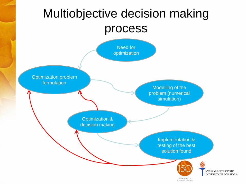
Multiobjective decision making
process
Need for
optimization
Optimization &
decision making
Optimization problem
formulation Modelling of the
problem (numerical
simulation)
Implementation &
testing of the best
solution found
Optimization problem formulation
By optimizing only one criterion, the rest
are not considered
Objective vs. constraint
Summation of the objectives
– adding apples and oranges
Converting the objectives (e.g. as costs)
– not easy, includes uncertaintes
Multiobjective formulation reveals
interdependences between the objectives
Example 1: Continuous casting of
steel
Optimal control of the secondary cooling of
continuous casting of steel
Long history of research in the Dept. of
Mathematical Information Technology,
Univ. of Jyväskylä
– modelling (1988)
– single objective optimization (1988-1994)
– multiobjective optimization (1994-1998)
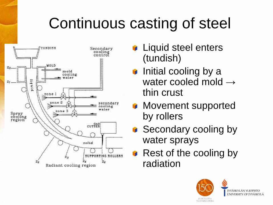
Continuous casting of steel
Liquid steel enters (tundish)
Initial cooling by a water cooled mold → thin crust
Movement supported by rollers
Secondary cooling by water sprays
Rest of the cooling by radiation
Continuous casting of steel
Measuring temperature in casting difficult →
numerical temperature distribution
Process modelled as a multiphase heat
equation (PDEs, solid & liquid phase) →
temperature distribution
Numerical model by using the finite element
method (FEM)
Dynamic process
Continuous casting of steel
Secondary cooling significant: intensity of sprays (easy to control) affects significantly to the solidification of steel
Goal: minimize the amount of defects in steel
Quality depends on e.g. the temperature distribution at the surface of steel – too slow cooling → too long liquid part
– too fast cooling → defects appear
Objective function: keep the surface temperature as close to a given profile as possible
Constraints e.g. for the change of temperature and for the temperature in critical spots
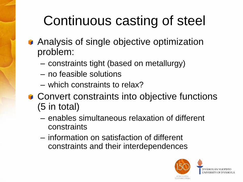
Continuous casting of steel
Analysis of single objective optimization problem: – constraints tight (based on metallurgy)
– no feasible solutions
– which constraints to relax?
Convert constraints into objective functions (5 in total) – enables simultaneous relaxation of different
constraints
– information on satisfaction of different constraints and their interdependences
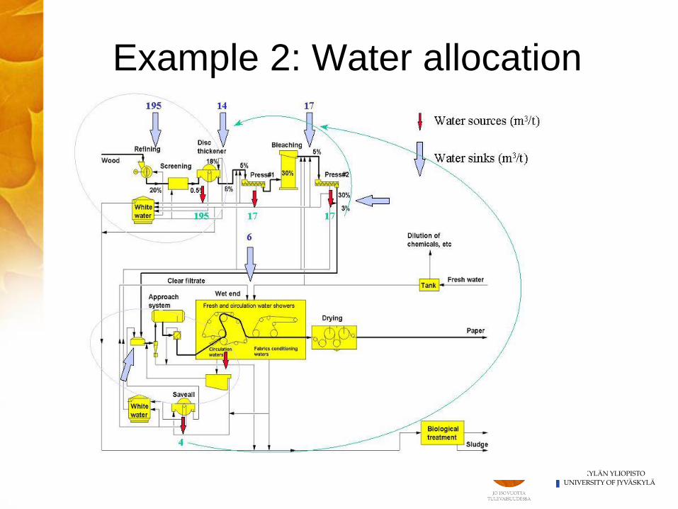
Example 2: Water allocation
Water allocation
Papermaking process consumes lots of water (nowadays about 5-10 m3/ton of paper)
Water can be circulated and reused in different parts of the process as long as it remains fresh enough – dissolved organic material accumulates
Fresh water costs
Process was modelles with the Balas process simulator (http://balas.vtt.fi/)
How to formulate the optimization problem?
Water allocation
Goal is to minimize the amount of fresh water required for the process
Objective function: minimize the amount of fresh water
Constraints – the amount of dissolved organic material in the
white water of the papermachine
– the amount of dissolved organic material in the pulp entering bleaching
Variables: 5 splitters ja 3 valves
Water allocation
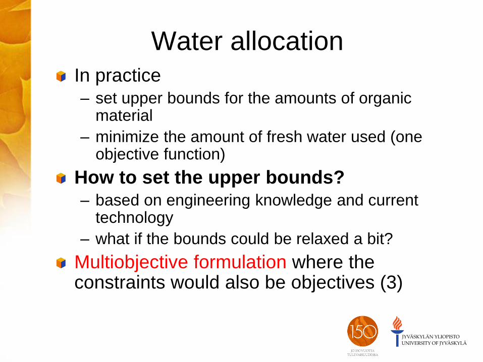
In practice – set upper bounds for the amounts of organic
material
– minimize the amount of fresh water used (one objective function)
How to set the upper bounds? – based on engineering knowledge and current
technology
– what if the bounds could be relaxed a bit?
Multiobjective formulation where the constraints would also be objectives (3)
Example 3: Chemical separation
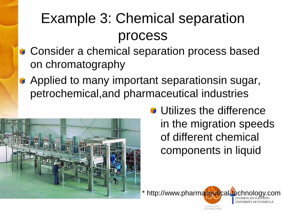
process Consider a chemical separation process based
on chromatography
Applied to many important separationsin sugar,
petrochemical,and pharmaceutical industries
* http://www.pharmaceutical-technology.com
Utilizes the difference
in the migration speeds
of different chemical
components in liquid
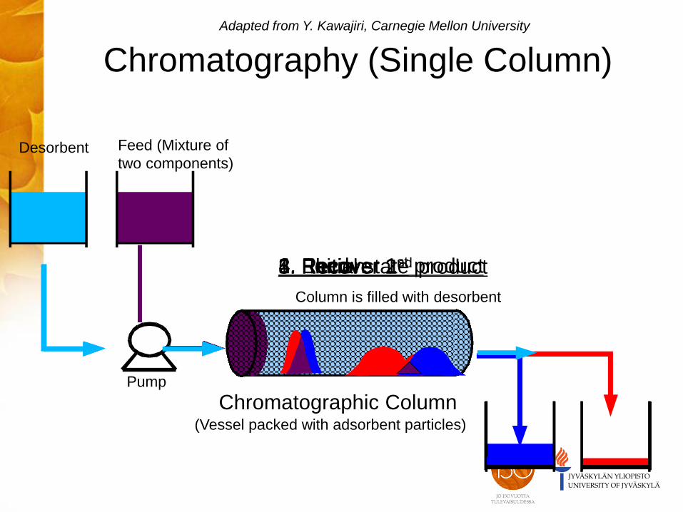
5. Recover 2nd product 4. Recover 1st product 2. Feed
Desorbent Feed (Mixture of
two components)
1. Initial state
Column is filled with desorbent
3. Elution
Chromatography (Single Column)
Chromatographic Column (Vessel packed with adsorbent particles)
Pump
Adapted from Y. Kawajiri, Carnegie Mellon University
November 11, 2009 Bergische Universität Wuppertal
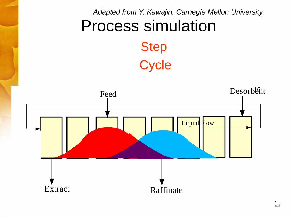
Process simulation
Cycle
Step
Liquid Flow
FeedDesorbent
Extract Raffinate
1
Liquid Flow
FeedDesorbent
Extract Raffinate
2
Liquid Flow
FeedDesorbent
Extract Raffinate
3
Liquid Flow
FeedDesorbent
Extract Raffinate
4
Liquid Flow
FeedDesorbent
Extract Raffinate
5
Liquid Flow
FeedDesorbent
Extract Raffinate
6
Liquid Flow
FeedDesorbent
ExtractRaffinate
7
Liquid Flow
FeedDesorbent
ExtractRaffinate
8
Liquid Flow
FeedDesorbent
ExtractRaffinate
9
Liquid Flow
FeedDesorbent
ExtractRaffinate
10
Liquid Flow
Feed Desorbent
ExtractRaffinate
11
Liquid Flow
Feed Desorbent
ExtractRaffinate
12
Liquid Flow
Feed Desorbent
ExtractRaffinate
13
Liquid Flow
Feed Desorbent
ExtractRaffinate
14
Liquid Flow
Feed Desorbent
Extract Raffinate
15
Liquid Flow
Feed Desorbent
Extract Raffinate
16
Adapted from Y. Kawajiri, Carnegie Mellon University
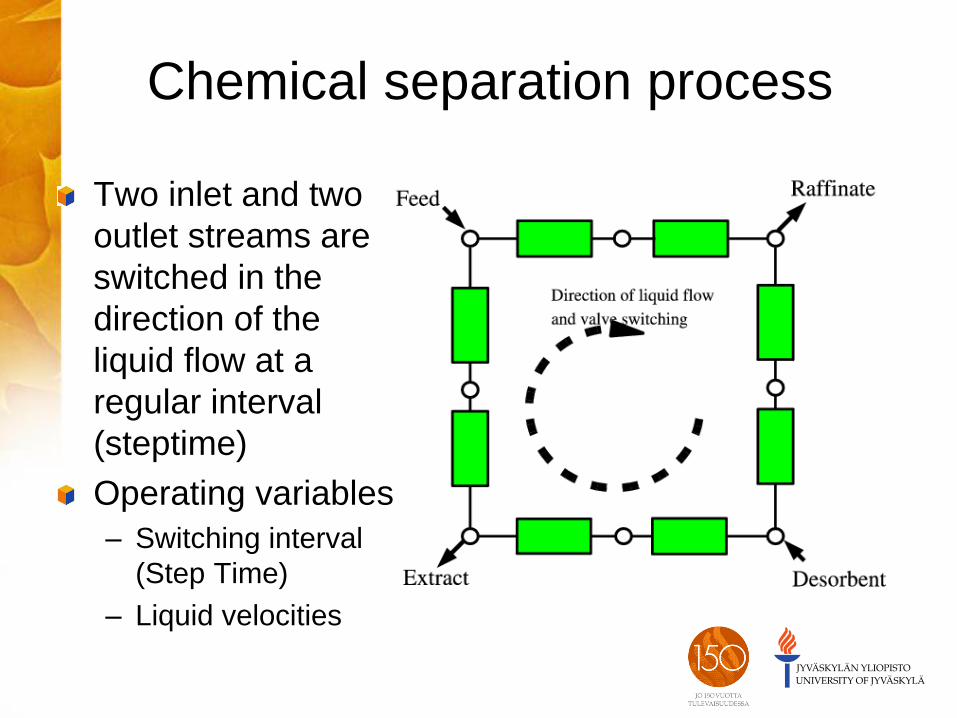
Chemical separation process
Two inlet and two
outlet streams are
switched in the
direction of the
liquid flow at a
regular interval
(steptime)
Operating variables
– Switching interval
(Step Time)
– Liquid velocities
Chemical separation process
Typically a profit function is optimized
Formulation of a profit is not easy
Multiobjective formulation – max throughput
– min desorbent consumption
– max purity of the product
– max recovery of the product
Enables more flexible consideration and reveals how different objectives affect the solution
Multiobjective optimization (MOO)
problem
Multiple objective functions, number denoted by k ( k > 1) – special case: two objectives
– Objective vectors can be visualized when k = 2, 3
Variables: values change the solution
Constraints: same as in single objective problems
Feasible region S: consists of all the points satisfying the constraints
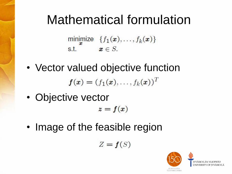
Mathematical formulation
• Vector valued objective function
• Objective vector
• Image of the feasible region
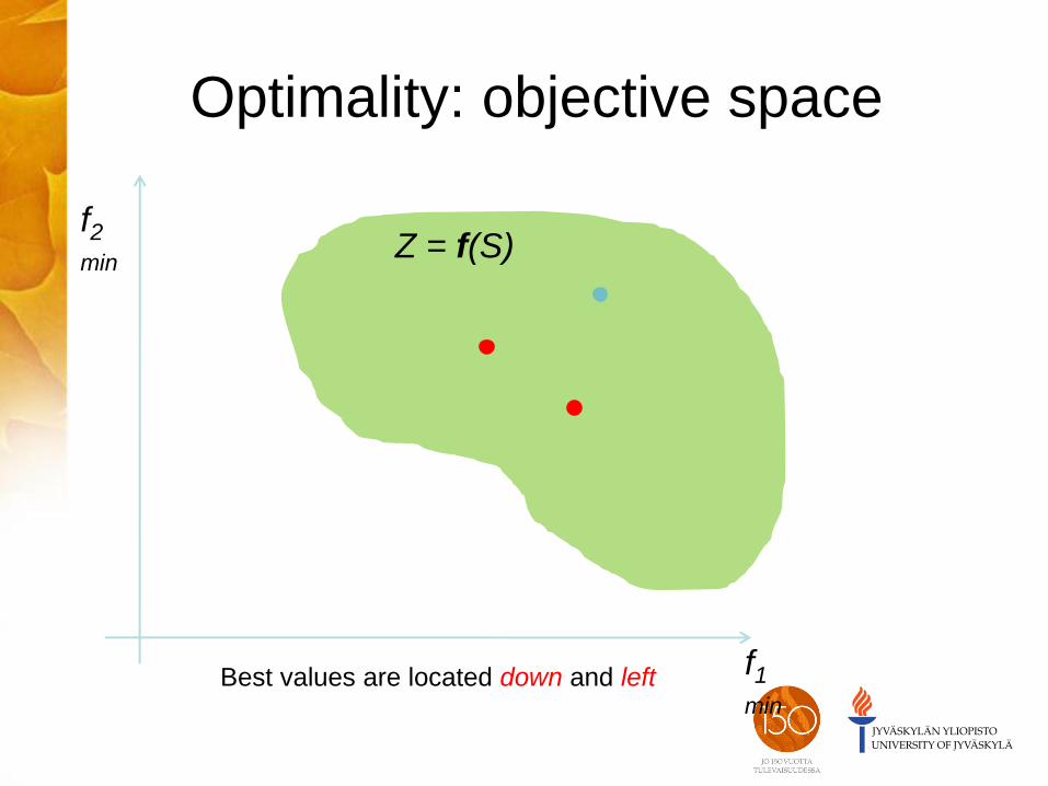
Optimality: objective space
f1
min
f2
min Z = f(S)
Best values are located down and left
Optimality for multiple objectives
When objectives to be optimized are
conflicting → no single optimal solution
– cf. single objective optimization
Compromise
There are potentially infinitely many optimal
solutions
Optimality
Which solutions can be ’’optimal’’?
How to find such solutions?
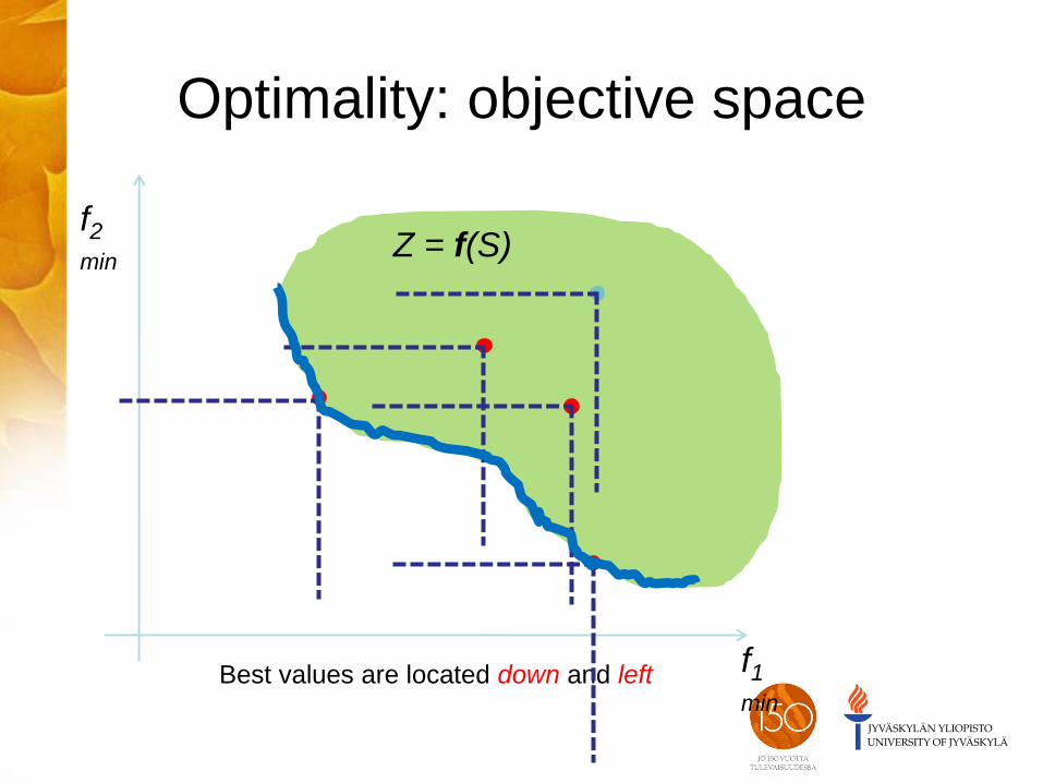
Optimality: objective space
f1
min
f2
min Z = f(S)
Best values are located down and left
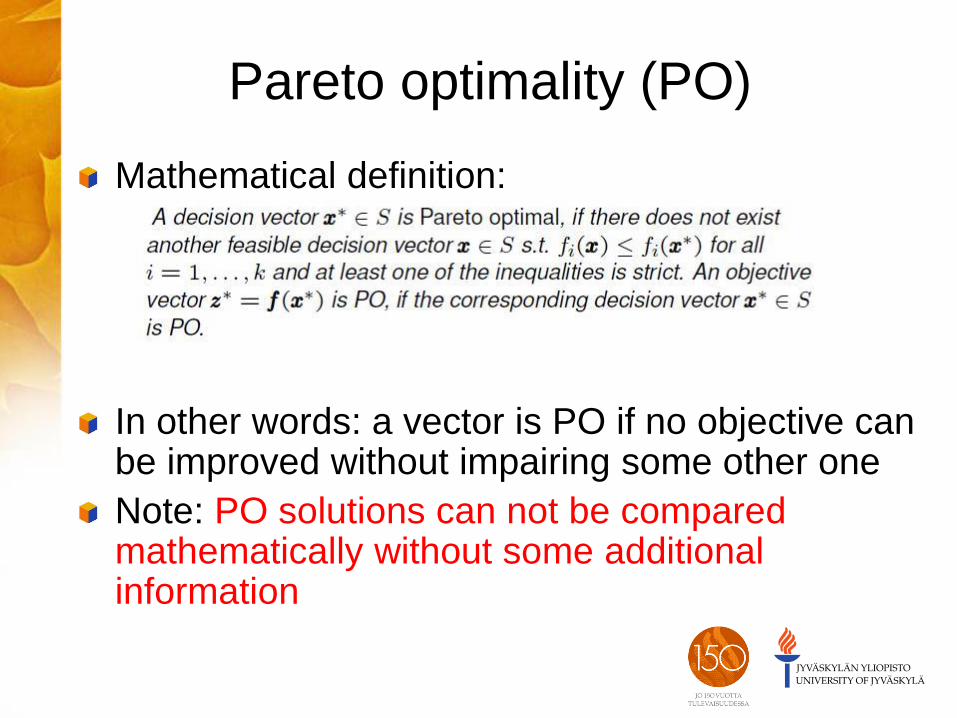
Pareto optimality (PO)
Mathematical definition:
In other words: a vector is PO if no objective can be improved without impairing some other one
Note: PO solutions can not be compared mathematically without some additional information
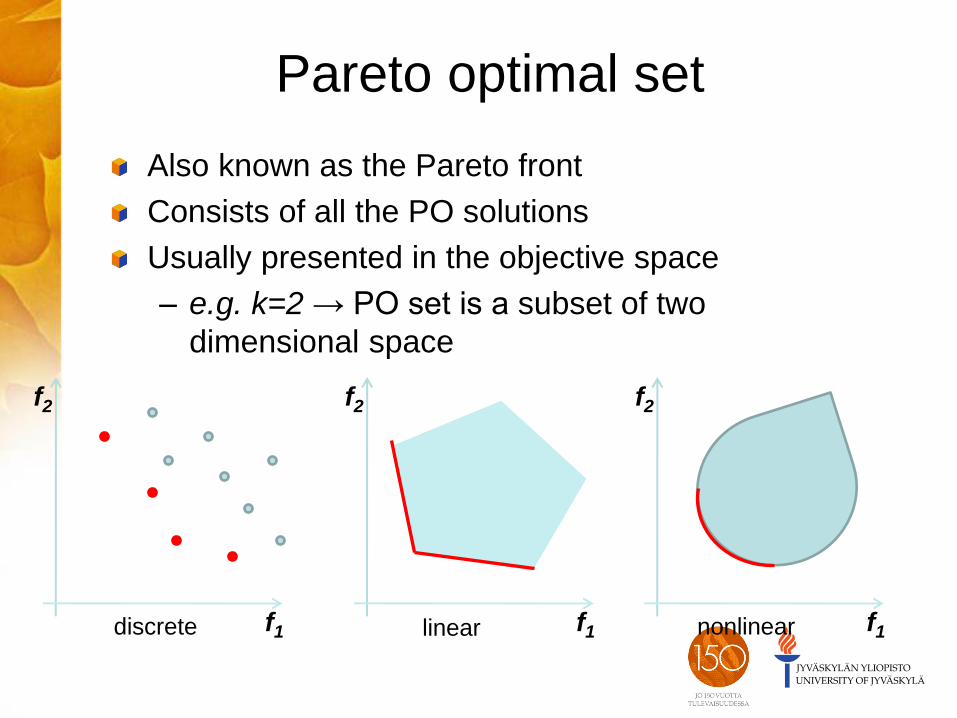
Pareto optimal set
Also known as the Pareto front
Consists of all the PO solutions
Usually presented in the objective space
– e.g. k=2 → PO set is a subset of two
dimensional space
f1
f2
f1
f2
f1
f2
discrete linear nonlinear
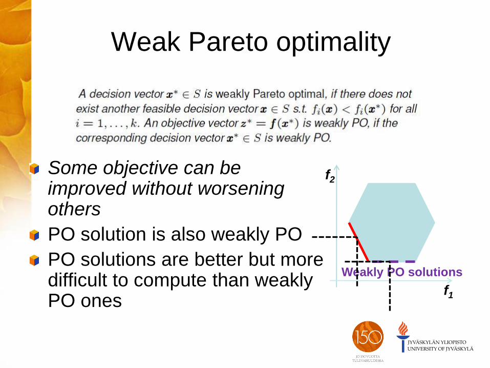
Weak Pareto optimality
Some objective can be improved without worsening others
PO solution is also weakly PO
PO solutions are better but more difficult to compute than weakly PO ones
Weakly PO solutions
f1
f2
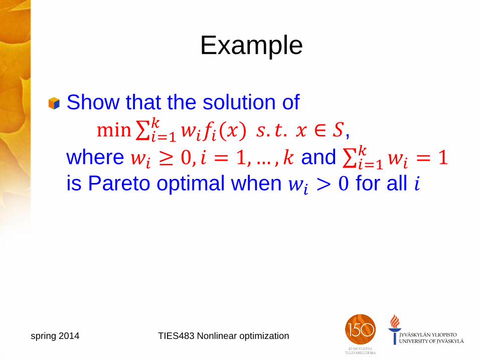
Example
Show that the solution of
min 𝑤𝑖𝑓𝑖(𝑥)𝑘𝑖=1 𝑠. 𝑡. 𝑥 ∈ 𝑆,
where 𝑤𝑖 ≥ 0, 𝑖 = 1,… , 𝑘 and 𝑤𝑖𝑘𝑖=1 = 1
is Pareto optimal when 𝑤𝑖 > 0 for all 𝑖
spring 2014 TIES483 Nonlinear optimization
What means solving a problem?
Find all PO solutions – theoretical approach, not feasible in practice
Find an approximation for PO front – approximation with good diversity
(representatives in all parts of the PO set) and good spread (no similar solutions)
– can also be an approximation of some specific part of the front
Find a best compromise (PO solution) – requires preferences from a DM
How to choose ’’a best’’
compromise?
PO solutions can not be compared
mathematically without some additional
information
– cf. ordering vectors in a plane
There typically exist infinitely many PO
solutions for continuous problems
Additional information related to the
problem considered is needed
Decision maker (DM)
Person(s) who is an expert in the
application area
Is able to express preferences related to
objectives
– e.g. is able to compare Pareto optimal solutions
No need for expertize in optimization
Helps in finding a best compromise
Ranges for the PO set
Ranges for the objective function values in
the PO set provide information about
achievable solutions
Ideal objective vector (best values)
– how good values can be obtained
Nadir objective vector (worst values)
– how bad values possibly have to be accepted
Usefull information in decision making
Are utilized also in some MOO methods
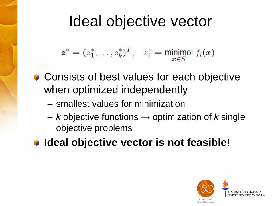
Ideal objective vector
Consists of best values for each objective
when optimized independently
– smallest values for minimization
– k objective functions → optimization of k single
objective problems
Ideal objective vector is not feasible!
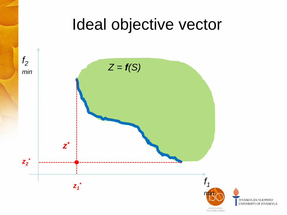
Ideal objective vector
f1
min
f2
min Z = f(S)
z2*
z1*
z*
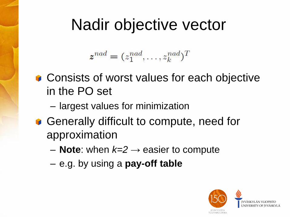
Nadir objective vector
Consists of worst values for each objective
in the PO set
– largest values for minimization
Generally difficult to compute, need for
approximation
– Note: when k=2 → easier to compute
– e.g. by using a pay-off table
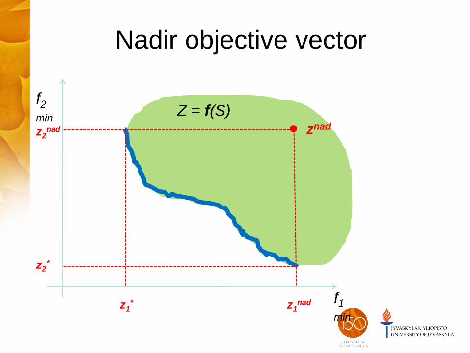
Nadir objective vector
f1
min
f2
min Z = f(S)
z2nad
z1nad
znad
z2*
z1*
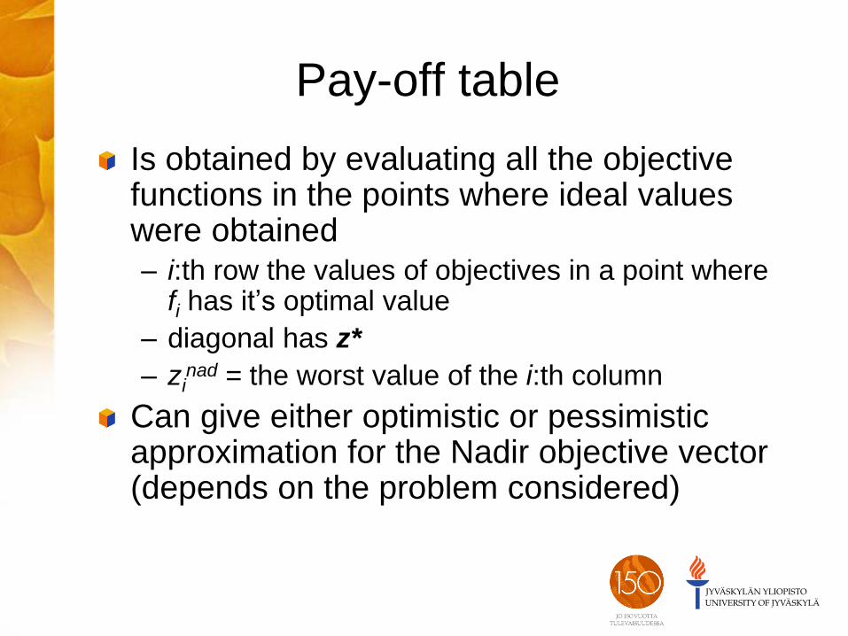
Pay-off table
Is obtained by evaluating all the objective functions in the points where ideal values were obtained – i:th row the values of objectives in a point where
fi has it’s optimal value
– diagonal has z*
– zinad = the worst value of the i:th column
Can give either optimistic or pessimistic approximation for the Nadir objective vector (depends on the problem considered)
Reference point
Reference point = a vector in the objective
space that contains desirable values for the
objectives
The components of a reference point are
called aspiration levels
One way for the DM to express preferences
(intuitive)
Utilized also in some MOO methods
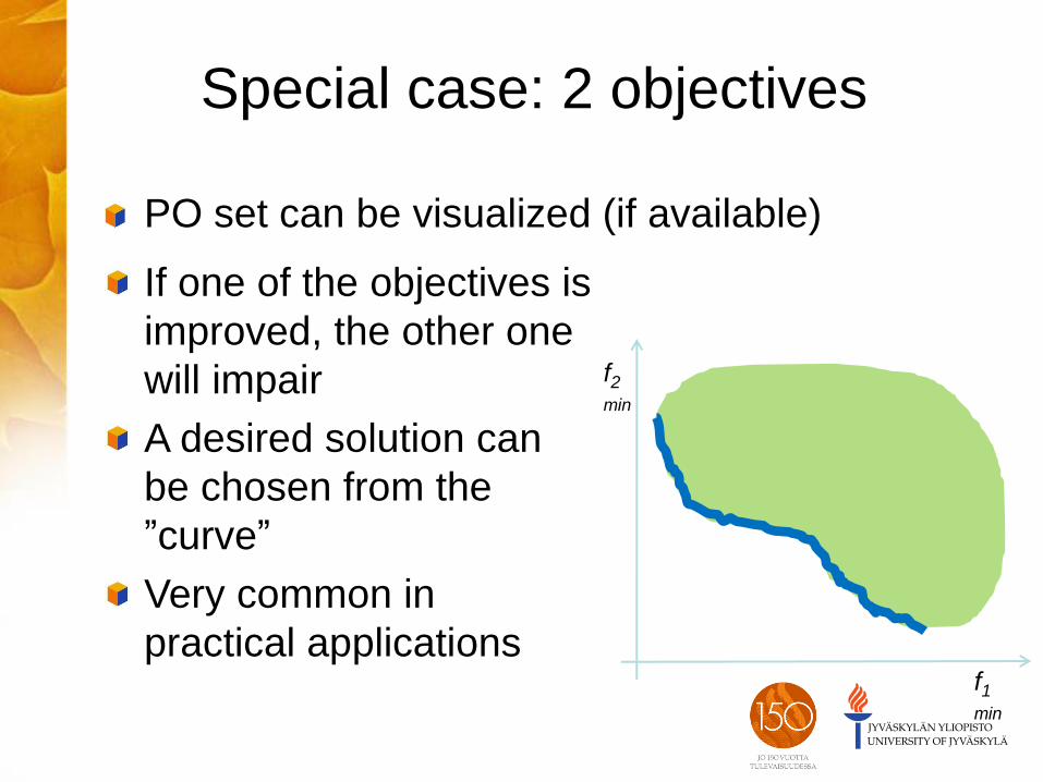
Special case: 2 objectives
PO set can be visualized (if available)
f1
min
f2
min
If one of the objectives is
improved, the other one
will impair
A desired solution can
be chosen from the
”curve”
Very common in
practical applications
Scalarizing the problem
Often the idea of MOO methods is to some way convert the problem into single objective one – methods of single objective optimization can be
utilized
This is called scalarization
Can be done in a good way or in a bad way – examples of scalarization will come in later
lectures
Properties of a good MOO method
Methods based on scalarization produce
usually one solution at a time
Good method should have the following
properties
– produce (weakly) PO solutions
– is able to find any (weakly) PO solution (by
using suitable parameters of the method)
Approaches
Plenty of methods developed for MOO
MOO methods can de categorized based
on the role of the DM
– No-preference methods (no DM)
– Aposteriori methods
– Apriori methods
– Interactive methods
Different categories are considered in
the next lecture!
Examples of MOO literature
V. Changkong & Y. Haimes, Multiobjective Decision Making: Theory and Methodology, 1983
Y. Sawaragi, H. Nakayama & T. Tanino, Theory of Multiobjective Optimization, 1985
R.E. Steuer, Multiple Criteria Optimization: Theory, Computation and Applications, 1986
K. Miettinen, Nonlinear Multiobjective Optimization, 1999
K. Deb, Multi-Objective Optimization Using Evolutionary Algorithms, 2001
Examples of MOO literature
M. Ehrgott, Multicriteria Optimization, 2005
J. Branke, K. Deb, K. Miettinen & R.
Slowinski (eds): Multiobjective Optimization:
Interactive and Evolutionary Approaches,
2008
G.P. Rangaiah (editor), Multi-Objective
Optimization: Techniques and Applications
in Chemical Engineering, 2009
E. Talbi, Metaheuristics: from Design to
Implementation, 2009