introduction to network theory - the computer laboratory
TRANSCRIPT

Introduction to Network Introduction to Network TheoryTheory

What is a Network?What is a Network?
Network = graphNetwork = graph Informally a Informally a graphgraph is a set of nodes joined by a set of lines or is a set of nodes joined by a set of lines or
arrows.arrows.
1 12 3
4 45 56 6
2 3

Graph-based representations
Representing a problem as a graph canprovide a different point of view
Representing a problem as a graph canmake a problem much simpler More accurately, it can provide the
appropriate tools for solving the problem
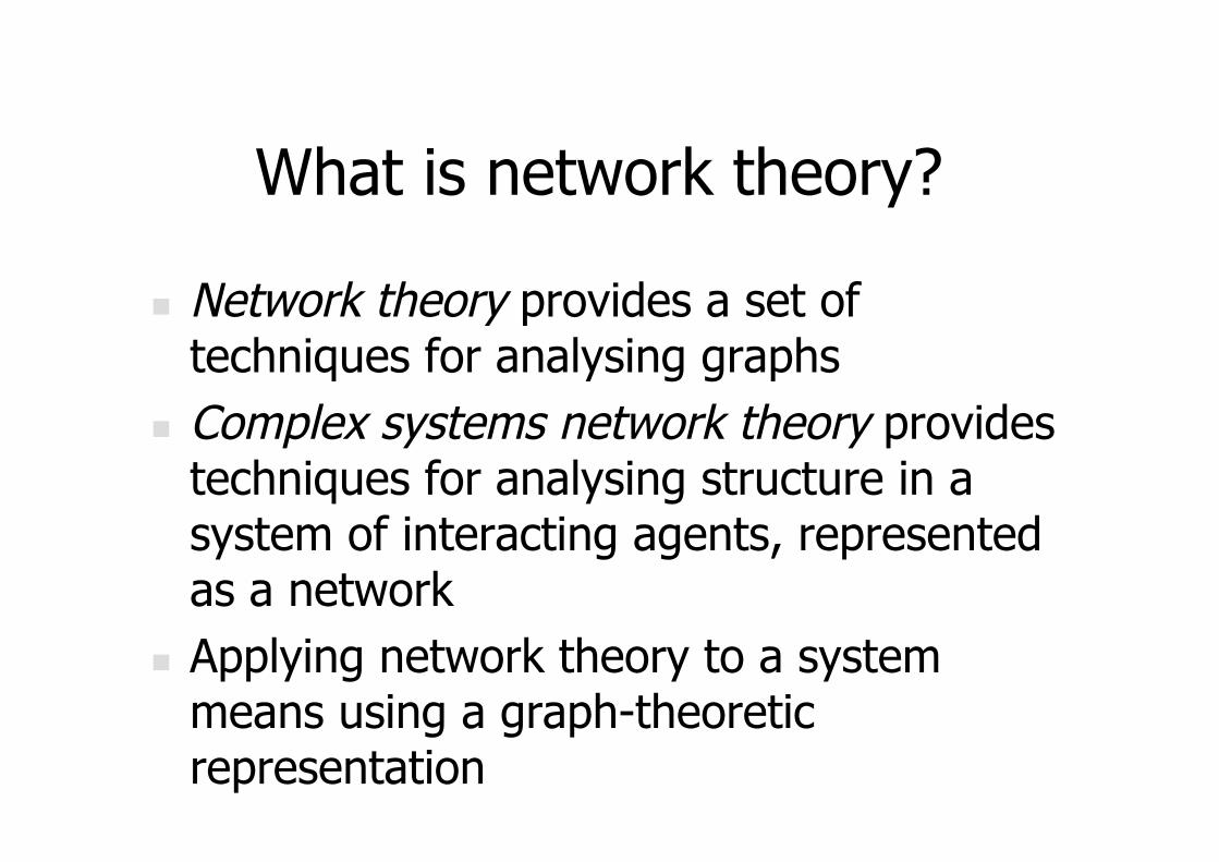
What is network theory?
Network theory provides a set oftechniques for analysing graphs
Complex systems network theory providestechniques for analysing structure in asystem of interacting agents, representedas a network
Applying network theory to a systemmeans using a graph-theoreticrepresentation
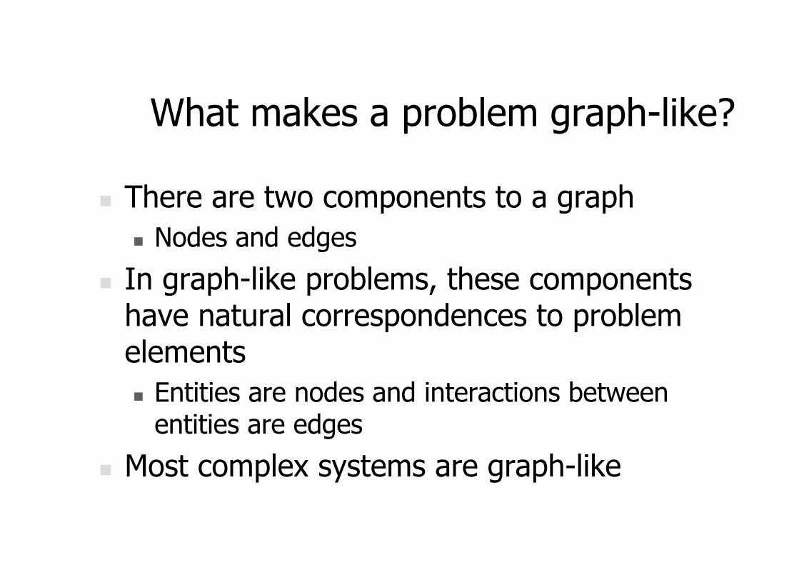
What makes a problem graph-like?
There are two components to a graph Nodes and edges
In graph-like problems, these componentshave natural correspondences to problemelements Entities are nodes and interactions between
entities are edges
Most complex systems are graph-like

Friendship Network

Scientific collaboration network

Business ties in US biotech-industry

Genetic interaction network
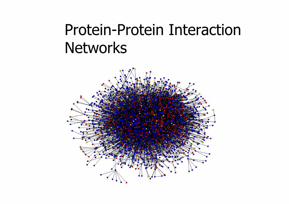
Protein-Protein InteractionNetworks

Transportation Networks
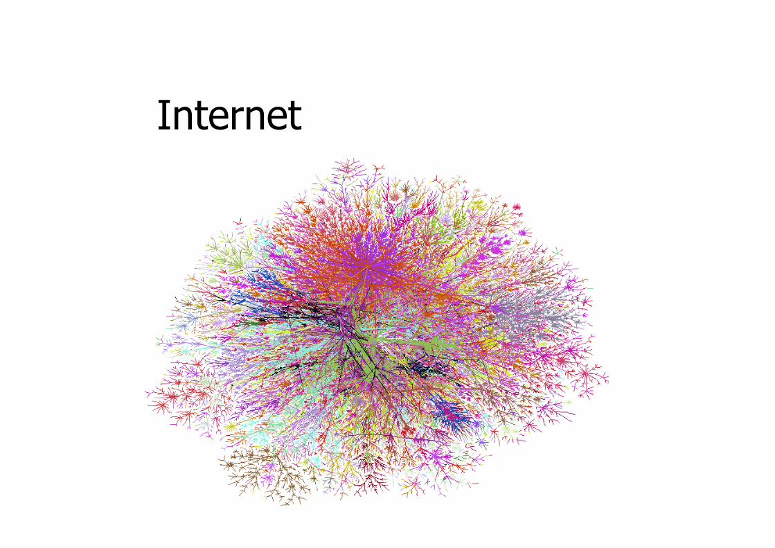
Internet
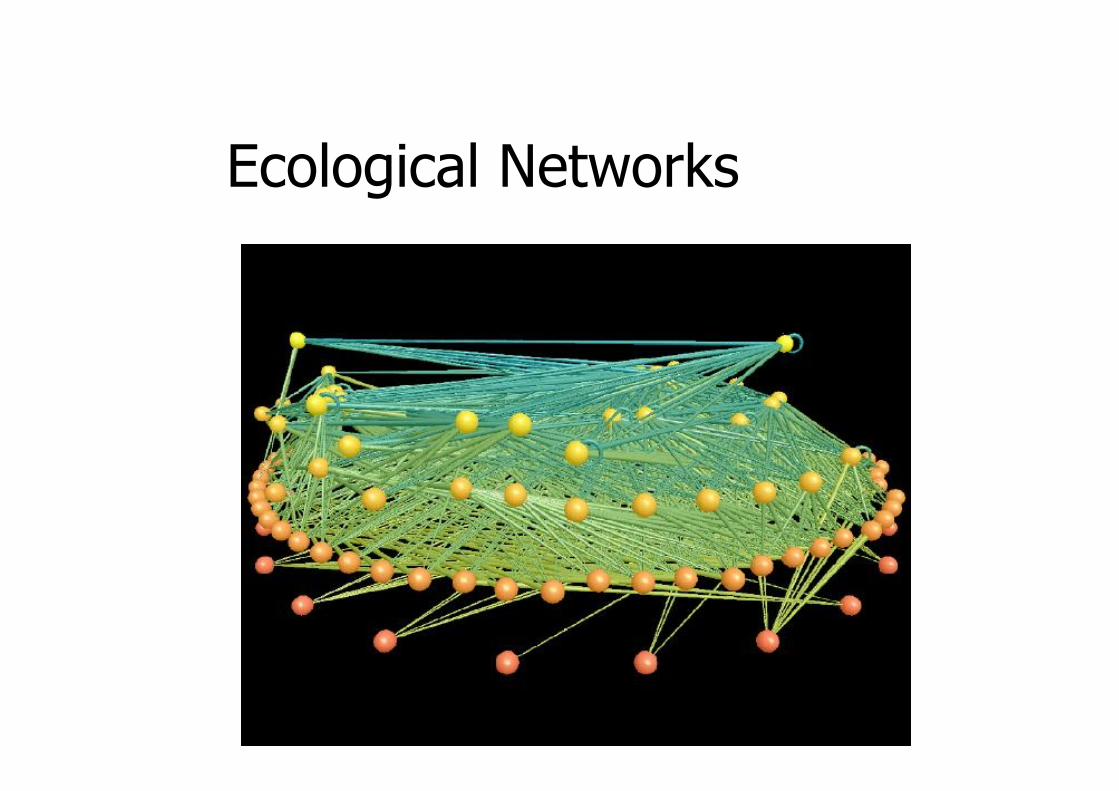
Ecological Networks

Graph Theory - HistoryGraph Theory - History
Leonhard Leonhard Euler's paper on Euler's paper on ““SevenSevenBridges of Bridges of KönigsbergKönigsberg”” , ,
published in 1736.published in 1736.
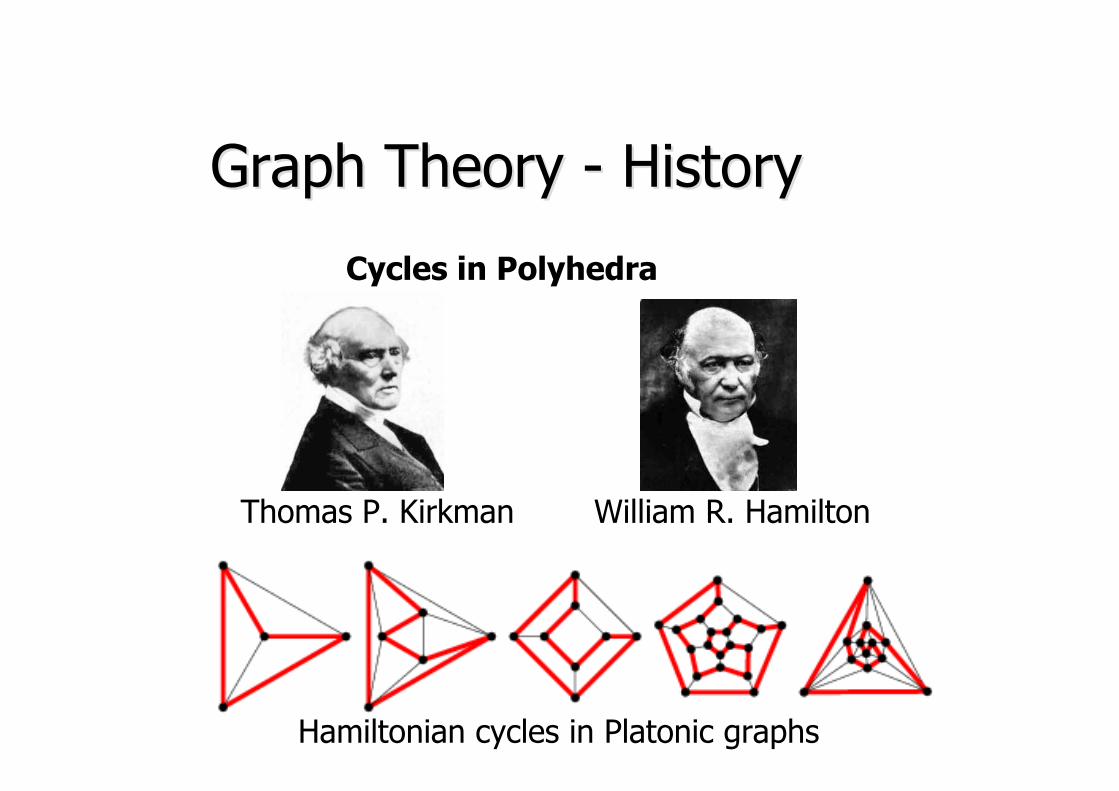
Graph Theory - HistoryGraph Theory - History
Cycles in Polyhedra
Thomas P. Kirkman William R. Hamilton
Hamiltonian cycles in Platonic graphs

Graph Theory - HistoryGraph Theory - History
Gustav Kirchhoff
Trees in Electric Circuits

Graph Theory - HistoryGraph Theory - History
Arthur Cayley James J. Sylvester George Polya
Enumeration of Chemical Isomers
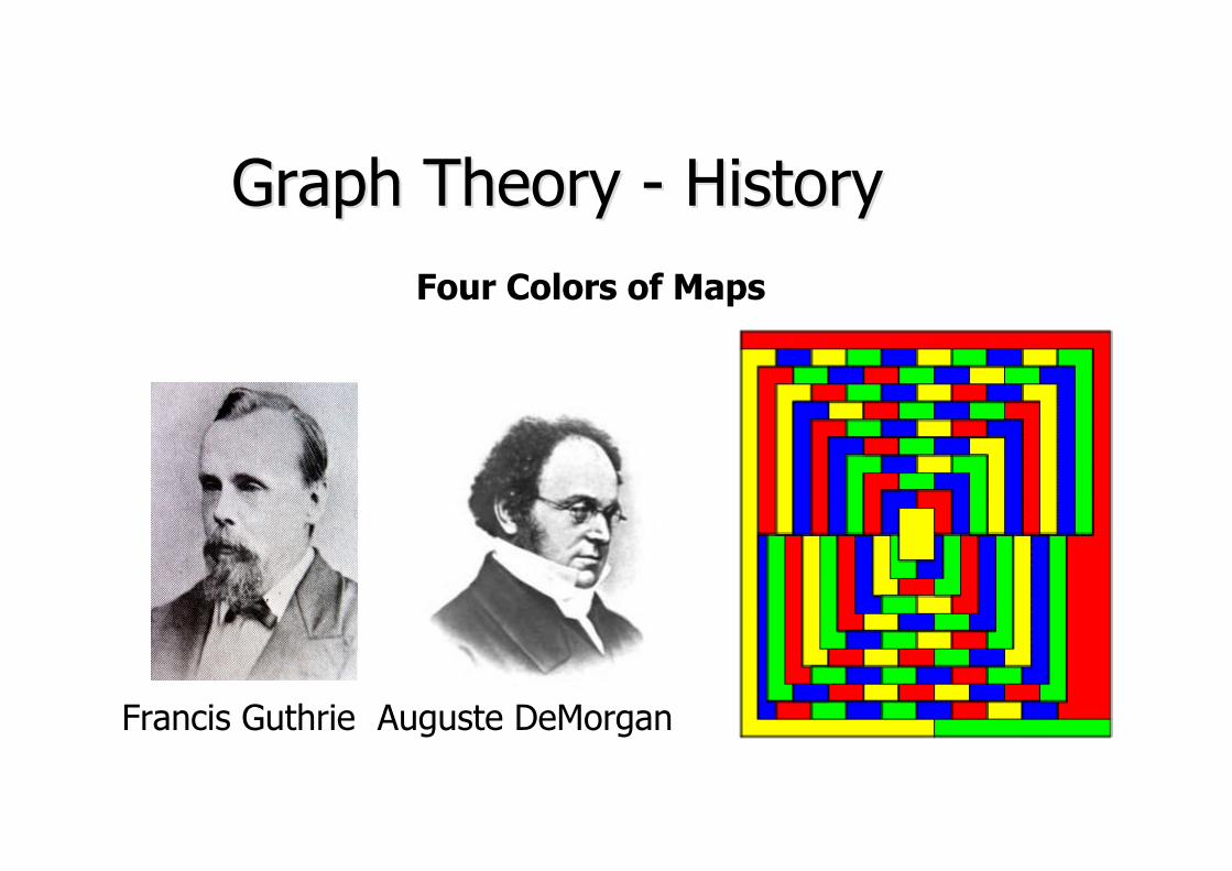
Graph Theory - HistoryGraph Theory - History
Francis Guthrie Auguste DeMorgan
Four Colors of Maps
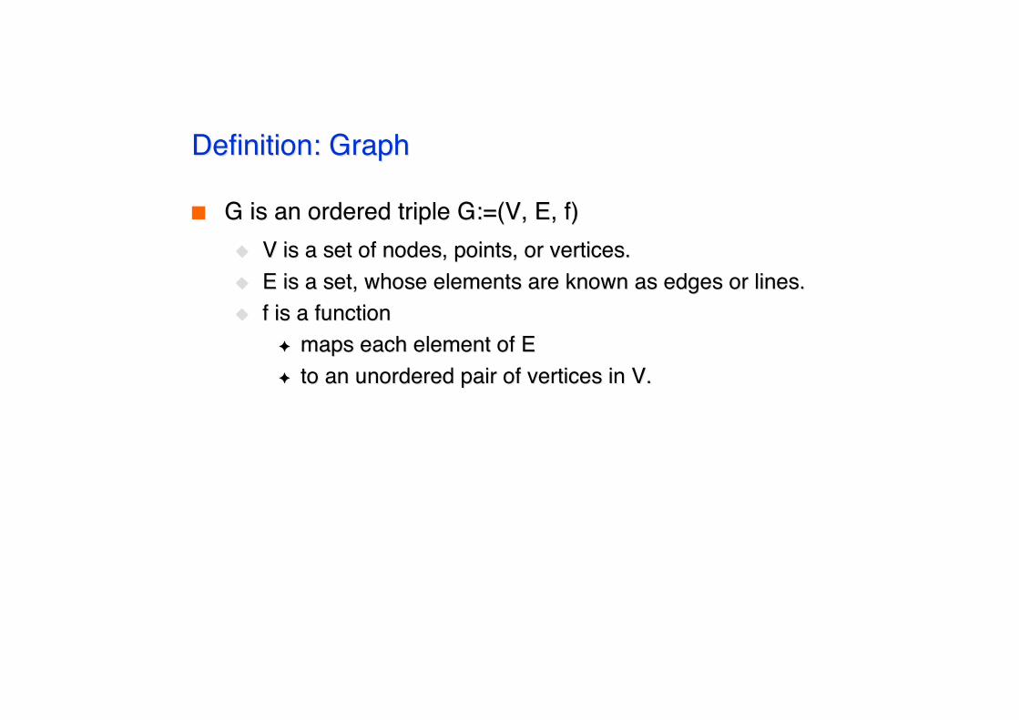
Definition: GraphDefinition: Graph
G is an ordered triple G:=(V, E, f)G is an ordered triple G:=(V, E, f) V is a set of nodes, points, or vertices.V is a set of nodes, points, or vertices. E is a set, whose elements are known as edges or lines.E is a set, whose elements are known as edges or lines. f is a functionf is a function
maps each element of Emaps each element of E to an unordered pair of vertices in V.to an unordered pair of vertices in V.
DefinitionsDefinitions
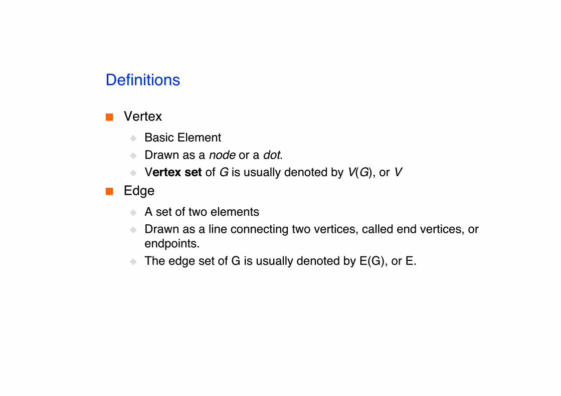
VertexVertex Basic ElementBasic Element Drawn as a Drawn as a nodenode or a or a dotdot.. VVertex setertex set of of GG is usually denoted by is usually denoted by VV((GG), or ), or VV
EdgeEdge A set of two elementsA set of two elements Drawn as a line connecting two vertices, called end vertices, orDrawn as a line connecting two vertices, called end vertices, or
endpoints.endpoints. The edge set of G is usually denoted by E(G), or E.The edge set of G is usually denoted by E(G), or E.

Example
V:={1,2,3,4,5,6}V:={1,2,3,4,5,6} E:={{1,2},{1,5},{2,3},{2,5},{3,4},{4,5},{4,6}}E:={{1,2},{1,5},{2,3},{2,5},{3,4},{4,5},{4,6}}

Simple Graphs
Simple graphsSimple graphs are graphs without multiple edges or self-loops. are graphs without multiple edges or self-loops.

Directed Graph (digraph)Directed Graph (digraph)
Edges have directionsEdges have directions An edge is an An edge is an ordered ordered pair of nodespair of nodes
loop
node
multiple arc
arc
Weighted graphs
1 2 3
4 5 6
.5
1.2
.2
.5
1.5.3
1
4 5 6
2 32
135
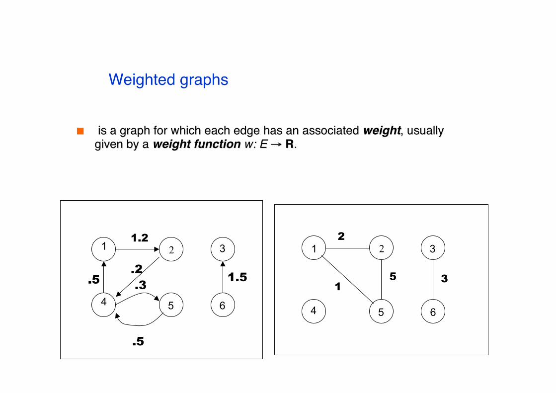
is a graph for which each edge has an associated is a graph for which each edge has an associated weightweight, usually, usuallygiven by a given by a weight functionweight function w: Ew: E →→ RR..

Structures and structuralmetrics
Graph structures are used to isolateinteresting or important sections of agraph
Structural metrics provide a measurementof a structural property of a graph Global metrics refer to a whole graph Local metrics refer to a single node in a graph

Graph structures
Identify interesting sections of a graph Interesting because they form a significant
domain-specific structure, or because theysignificantly contribute to graph properties
A subset of the nodes and edges in agraph that possess certain characteristics,or relate to each other in particular ways
Connectivity
a graph is a graph is connectedconnected if if you can get from any node to any other by following a sequence of edgesyou can get from any node to any other by following a sequence of edges
OROR any two nodes are connected by a path.any two nodes are connected by a path.
A directed graph is A directed graph is strongly connectedstrongly connected if there is a directed path from if there is a directed path fromany node to any other node.any node to any other node.

ComponentComponent
Every disconnected graph can be split up into a number ofEvery disconnected graph can be split up into a number ofconnected connected componentscomponents..
DegreeDegree
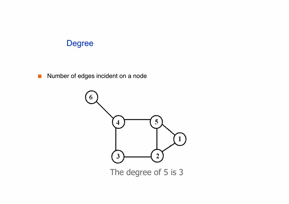
Number of edges incident on a nodeNumber of edges incident on a node
The degree of 5 is 3
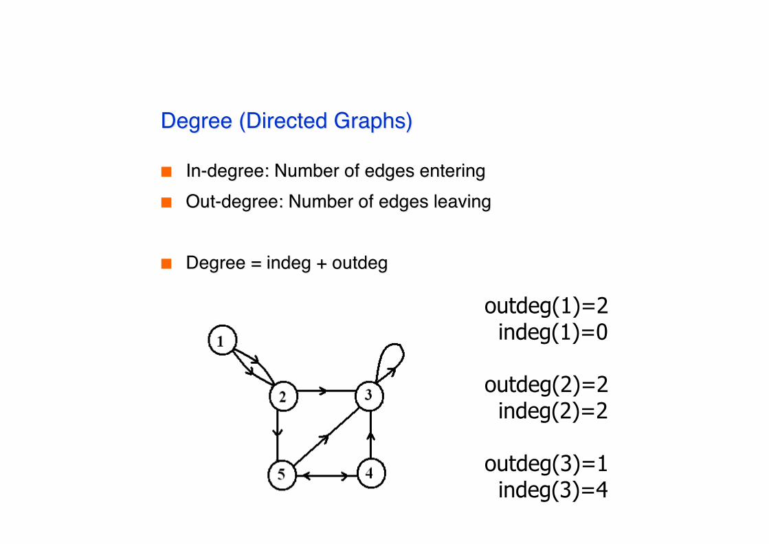
Degree (Directed Graphs)Degree (Directed Graphs)
In-degree: Number of edges enteringIn-degree: Number of edges entering Out-degree: Number of edges leavingOut-degree: Number of edges leaving
Degree = Degree = indeg indeg + + outdegoutdeg
outdeg(1)=2 indeg(1)=0
outdeg(2)=2 indeg(2)=2
outdeg(3)=1 indeg(3)=4

Degree: Simple Facts
If If G G is a graph with is a graph with mm edges, then edges, thenΣΣ deg( deg(vv) = 2) = 2mm = 2 |= 2 |EE | |
If If G G is a digraph then is a digraph thenΣΣ indegindeg((vv)=)=ΣΣ outdegoutdeg((vv) ) = = ||EE | |
Number of Odd degree Nodes is evenNumber of Odd degree Nodes is even
Walks
A walk of length k in a graph is a succession of k(not necessarily different) edges of the form
uv,vw,wx,…,yz.
This walk is denote by uvwx…xz, and is referred toas a walk between u and z.
A walk is closed is u=z.

PathPath
A A pathpath is a walk in which all the edges and all the nodes are different. is a walk in which all the edges and all the nodes are different.
Walks and Paths 1,2,5,2,3,4 1,2,5,2,3,2,1 1,2,3,4,6
walk of length 5 CW of length 6 path of length 4

Cycle
A A cyclecycle is a closed path in which all the edges are different. is a closed path in which all the edges are different.
1,2,5,1 2,3,4,5,23-cycle 4-cycle

Special Types of Graphs
Empty Graph / Edgeless graphEmpty Graph / Edgeless graph No edgeNo edge
Null graphNull graph No nodesNo nodes Obviously no edgeObviously no edge
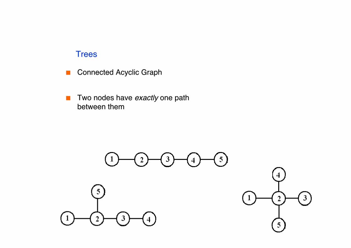
TreesTrees
Connected Acyclic GraphConnected Acyclic Graph
Two nodes have Two nodes have exactlyexactly one path one pathbetween thembetween them
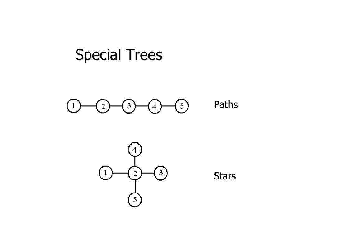
Special TreesSpecial Trees
Paths
Stars
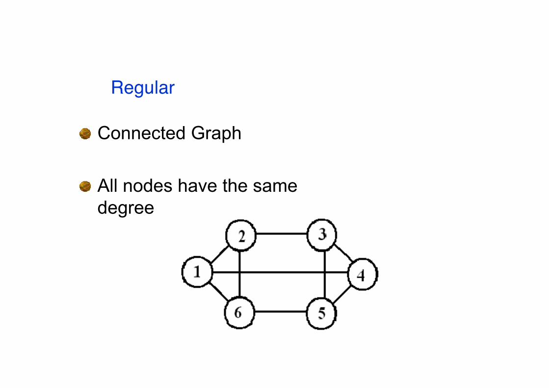
Connected Graph
All nodes have the samedegree
Regular
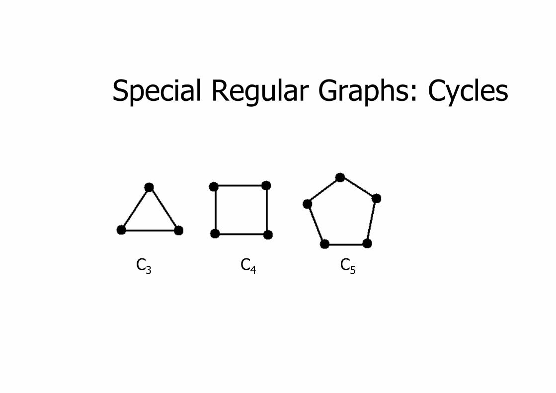
Special Regular Graphs: Cycles
C3 C4 C5
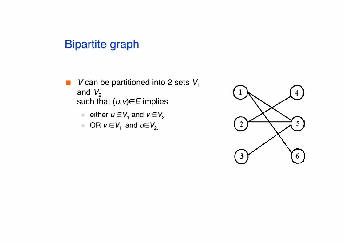
BipartiteBipartite graphgraph
VV can be partitioned into 2 sets can be partitioned into 2 sets VV11and and VV22such that (such that (uu,,vv))∈∈EE implies implies either either uu ∈∈VV11 and and vv ∈∈VV22
OR OR vv ∈∈VV1 1 and and uu∈∈VV2.2.

Complete GraphComplete Graph
Every pair of vertices are adjacentEvery pair of vertices are adjacent Has n(n-1)/2 edgesHas n(n-1)/2 edges

Complete Bipartite GraphComplete Bipartite Graph
Bipartite Variation of Complete GraphBipartite Variation of Complete Graph Every node of one set is connected to every other node on theEvery node of one set is connected to every other node on the
other setother set
Stars
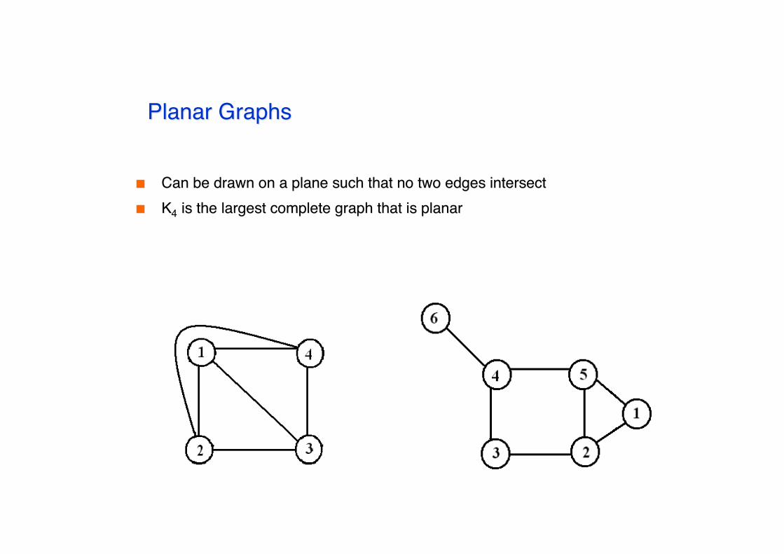
Planar GraphsPlanar Graphs
Can be drawn on a plane such that no two edges intersectCan be drawn on a plane such that no two edges intersect KK44 is the largest complete graph that is planar is the largest complete graph that is planar
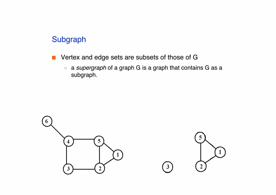
SubgraphSubgraph
Vertex and edge sets are subsets of those of GVertex and edge sets are subsets of those of G a a supergraphsupergraph of a graph G is a graph that contains G as a of a graph G is a graph that contains G as a
subgraphsubgraph..

Special Special SubgraphsSubgraphs: Cliques: Cliques
A clique is a maximum completeconnected subgraph..
A B
D
H
FE
C
IG

Spanning Spanning subgraphsubgraph
SubgraphSubgraph H has the same vertex set as G. H has the same vertex set as G. Possibly not all the edgesPossibly not all the edges ““H spans GH spans G””..

Spanning treeSpanning tree
Let G be a connected graph. Then aLet G be a connected graph. Then aspanning treespanning tree in G is a in G is a subgraphsubgraph of G of Gthat includes every node and is also athat includes every node and is also atree.tree.
IsomorphismIsomorphism
BijectionBijection, i.e., a one-to-one mapping:, i.e., a one-to-one mapping:f : V(G) -> V(H)f : V(G) -> V(H)
u and v from G are adjacent if and only if f(u) and f(v) areu and v from G are adjacent if and only if f(u) and f(v) areadjacent in H.adjacent in H.
If an isomorphism can be constructed between two graphs, thenIf an isomorphism can be constructed between two graphs, thenwe say those graphs are we say those graphs are isomorphicisomorphic..
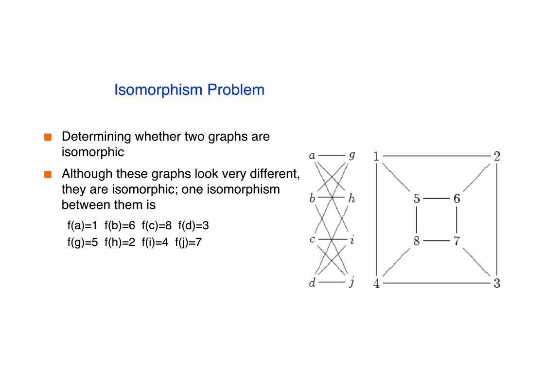
Isomorphism ProblemIsomorphism Problem
Determining whether two graphs areDetermining whether two graphs areisomorphicisomorphic
Although these graphs look very different,Although these graphs look very different,they are isomorphic; one isomorphismthey are isomorphic; one isomorphismbetween them isbetween them isf(a)=1 f(b)=6 f(c)=8 f(d)=3f(a)=1 f(b)=6 f(c)=8 f(d)=3f(g)=5 f(h)=2 f(i)=4 f(j)=7f(g)=5 f(h)=2 f(i)=4 f(j)=7
Representation (Matrix)Representation (Matrix)
Incidence MatrixIncidence Matrix V x EV x E [vertex, edges] contains the edge's data[vertex, edges] contains the edge's data
Adjacency MatrixAdjacency Matrix V x VV x V Boolean values (adjacent or not)Boolean values (adjacent or not) Or Edge WeightsOr Edge Weights

MatricesMatrices
1000000601010105111000040010100300011012000001116,45,44,35,23,25,12,1
001000600101151101004001010301010120100101654321

Representation (List)Representation (List)
Edge ListEdge List pairs (ordered if directed) of verticespairs (ordered if directed) of vertices Optionally weight and other dataOptionally weight and other data
Adjacency List (node list)Adjacency List (node list)
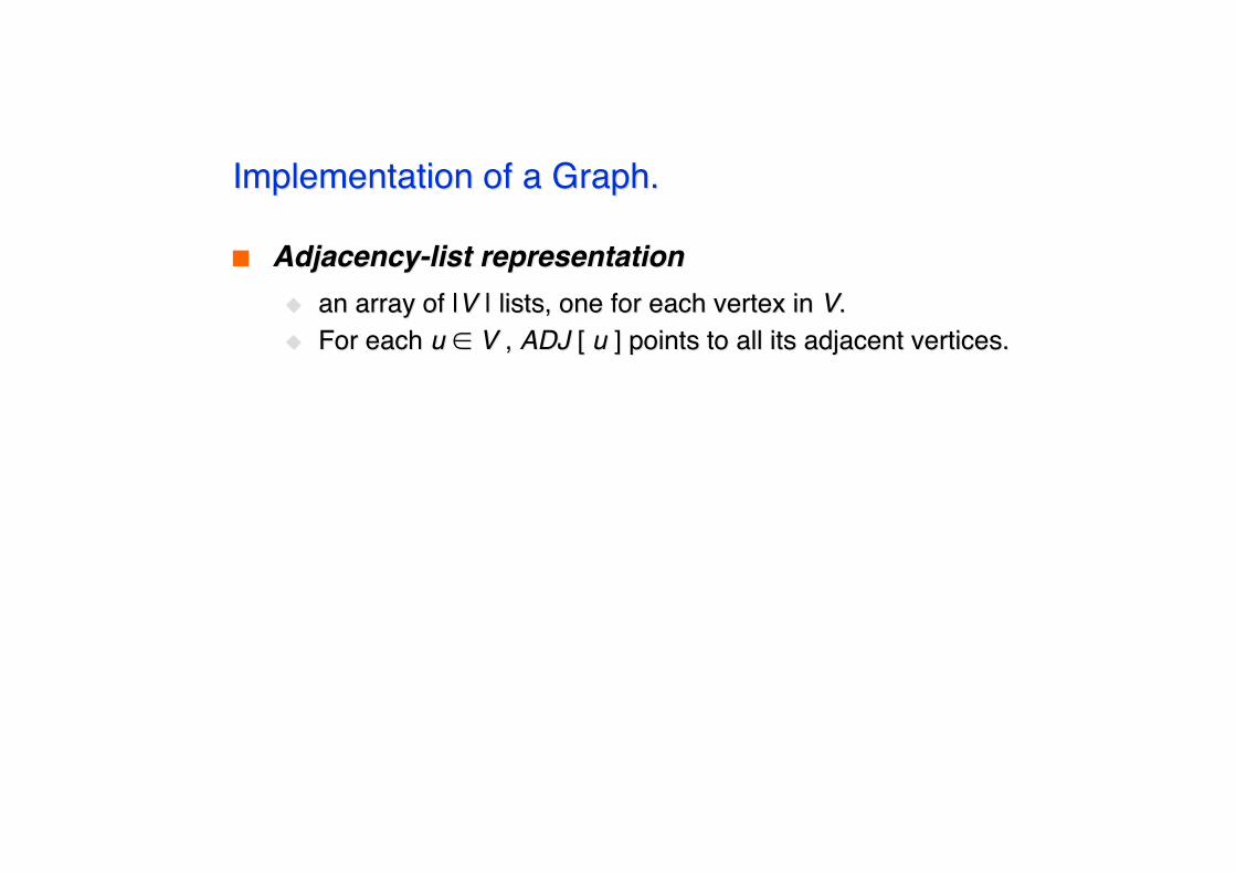
Implementation of a Graph.Implementation of a Graph.
Adjacency-list representationAdjacency-list representation an array of |an array of |VV | lists, one for each vertex in | lists, one for each vertex in VV.. For each For each uu ∈∈ VV , , ADJADJ [ [ uu ] points to all its adjacent vertices. ] points to all its adjacent vertices.
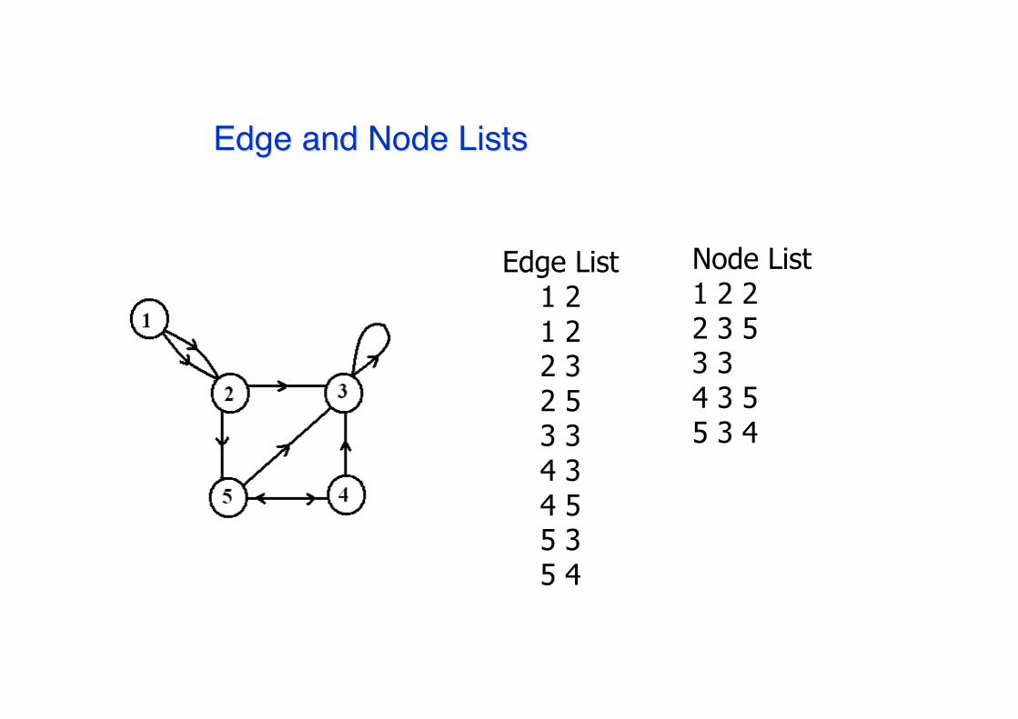
Edge and Node ListsEdge and Node Lists
Edge List1 21 22 32 53 34 34 55 35 4
Node List1 2 22 3 53 34 3 55 3 4
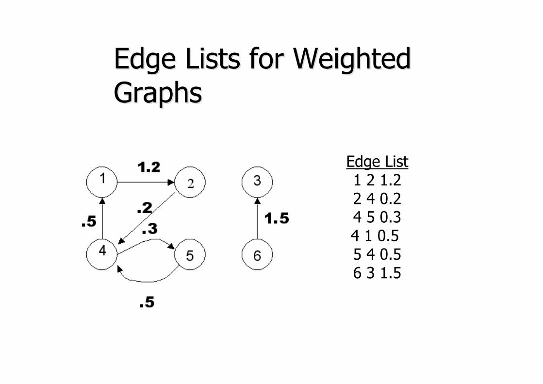
Edge List1 2 1.22 4 0.24 5 0.34 1 0.5 5 4 0.56 3 1.5
Edge Lists for WeightedEdge Lists for WeightedGraphsGraphs

Topological Distance
A shortest path is the minimum pathA shortest path is the minimum pathconnecting two nodes.connecting two nodes.
The number of edges in the shortest pathThe number of edges in the shortest pathconnecting connecting pp and and qq is the is the topologicaltopologicaldistancedistance between these two nodes, between these two nodes, ddpp,q,q
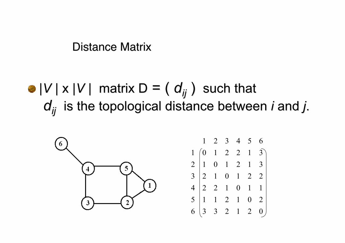
||VV | x | | x |V |V | matrix D matrix D = ( = ( ddijij )) such that such that ddijij is the topological distance between is the topological distance between ii and and jj..
021233620121151101224221012331210123122101654321
Distance MatrixDistance Matrix
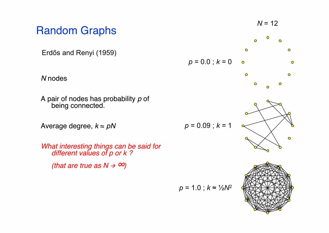
Random Graphs
N N nodesnodes
A pair of nodes has probability A pair of nodes has probability p p ofofbeing connected.being connected.
Average degree, Average degree, k k ≈≈ pNpN
What interesting things can be said forWhat interesting things can be said fordifferent values of p or k ?different values of p or k ?
(that are true as N (that are true as N ∞∞))
Erdős and Renyi (1959)p = 0.0 ; k = 0
N = 12
p = 0.09 ; k = 1
p = 1.0 ; k ≈ ½N2

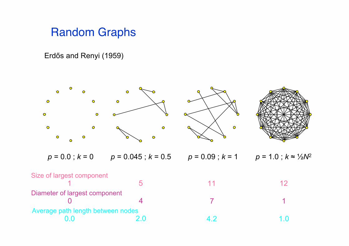
Random GraphsErdős and Renyi (1959)
p = 0.0 ; k = 0
p = 0.09 ; k = 1
p = 1.0 ; k ≈ ½N2
p = 0.045 ; k = 0.5
Let’s look at…
Size of the largest connected cluster
Diameter (maximum path length between nodes) of the largest cluster
Average path length between nodes (if a path exists)
Random Graphs
Erdős and Renyi (1959)
p = 0.0 ; k = 0 p = 0.09 ; k = 1 p = 1.0 ; k ≈ ½N2p = 0.045 ; k = 0.5
Size of largest component
Diameter of largest component
Average path length between nodes
1 5 11 12
0 4 7 1
0.0 2.0 4.2 1.0
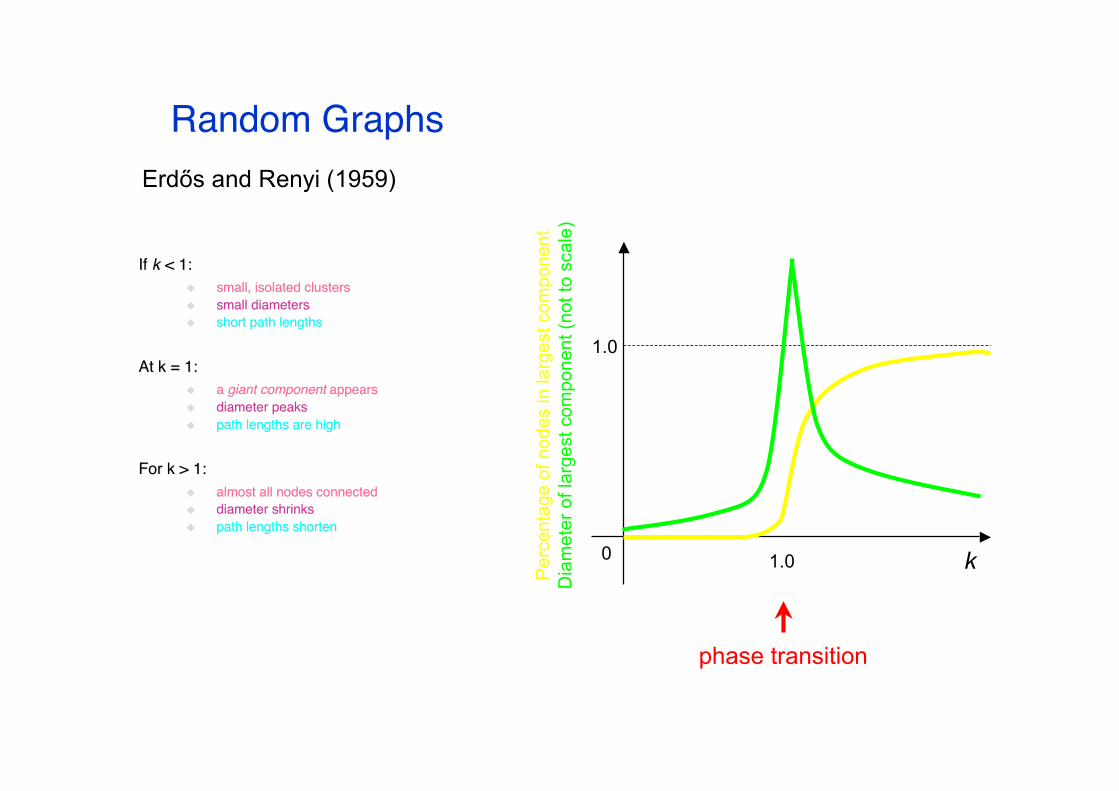
Random Graphs
If If kk < 1: < 1: small, isolated clusterssmall, isolated clusters small diameterssmall diameters short path lengthsshort path lengths
At k = 1:At k = 1: aa giant component giant component appearsappears diameter peaksdiameter peaks path lengths are highpath lengths are high
For k > 1:For k > 1: almost all nodes connectedalmost all nodes connected diameter shrinksdiameter shrinks path lengths shortenpath lengths shorten
Erdős and Renyi (1959)
Per
cent
age
of n
odes
in la
rges
t com
pone
ntD
iam
eter
of l
arge
st c
ompo
nent
(not
to s
cale
)
1.0
0 k1.0
phase transition
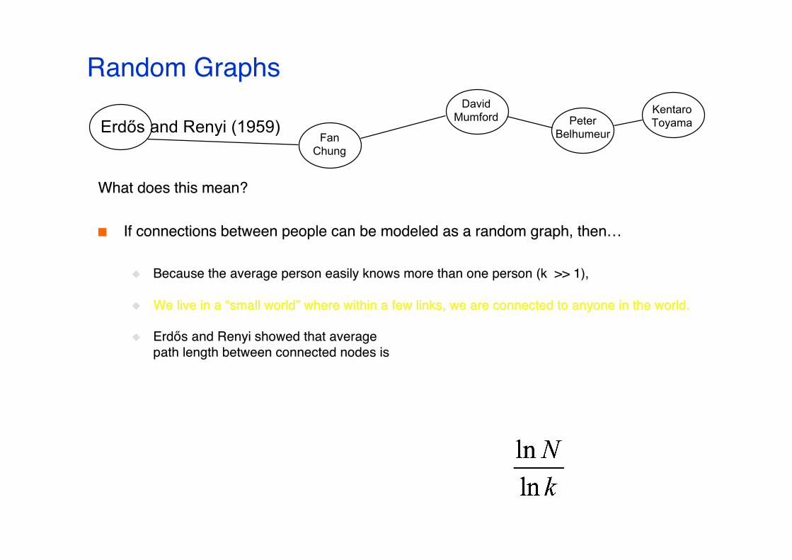
Random Graphs
What does this mean?What does this mean?
If connections between people can be modeled as a random graph, thenIf connections between people can be modeled as a random graph, then……
Because the average person easily knows more than one person (k >> 1),Because the average person easily knows more than one person (k >> 1),
We live in a We live in a ““small worldsmall world”” where within a few links, we are connected to anyone in the world. where within a few links, we are connected to anyone in the world.
ErdErdőős s and and Renyi Renyi showed that averageshowed that averagepath length between connected nodes ispath length between connected nodes is
Erdős and Renyi (1959)David
Mumford PeterBelhumeur
KentaroToyama
FanChung

Random Graphs
What does this mean?What does this mean?
If connections between people can be modeled as a random graph, thenIf connections between people can be modeled as a random graph, then……
Because the average person easily knows more than one person (k >> 1),Because the average person easily knows more than one person (k >> 1),
We live in a We live in a ““small worldsmall world”” where within a few links, we are connected to anyone in the world. where within a few links, we are connected to anyone in the world.
ErdErdőős s and and Renyi Renyi computed averagecomputed averagepath length between connected nodes to be:path length between connected nodes to be:
Erdős and Renyi (1959)David
Mumford PeterBelhumeur
KentaroToyama
FanChung
BIG “IF”!!!

The Alpha Model
The people you know arenThe people you know arenʼ̓t randomly chosen.t randomly chosen.
People tend to get to know those who are twoPeople tend to get to know those who are twolinks away (links away (Rapoport Rapoport **, 1957)., 1957).
The real world exhibits a lot of The real world exhibits a lot of clustering.clustering.
Watts (1999)
* Same Anatol Rapoport, known for TIT FOR TAT!
The Personal Mapby MSR Redmond’s Social Computing Group
The Alpha Model
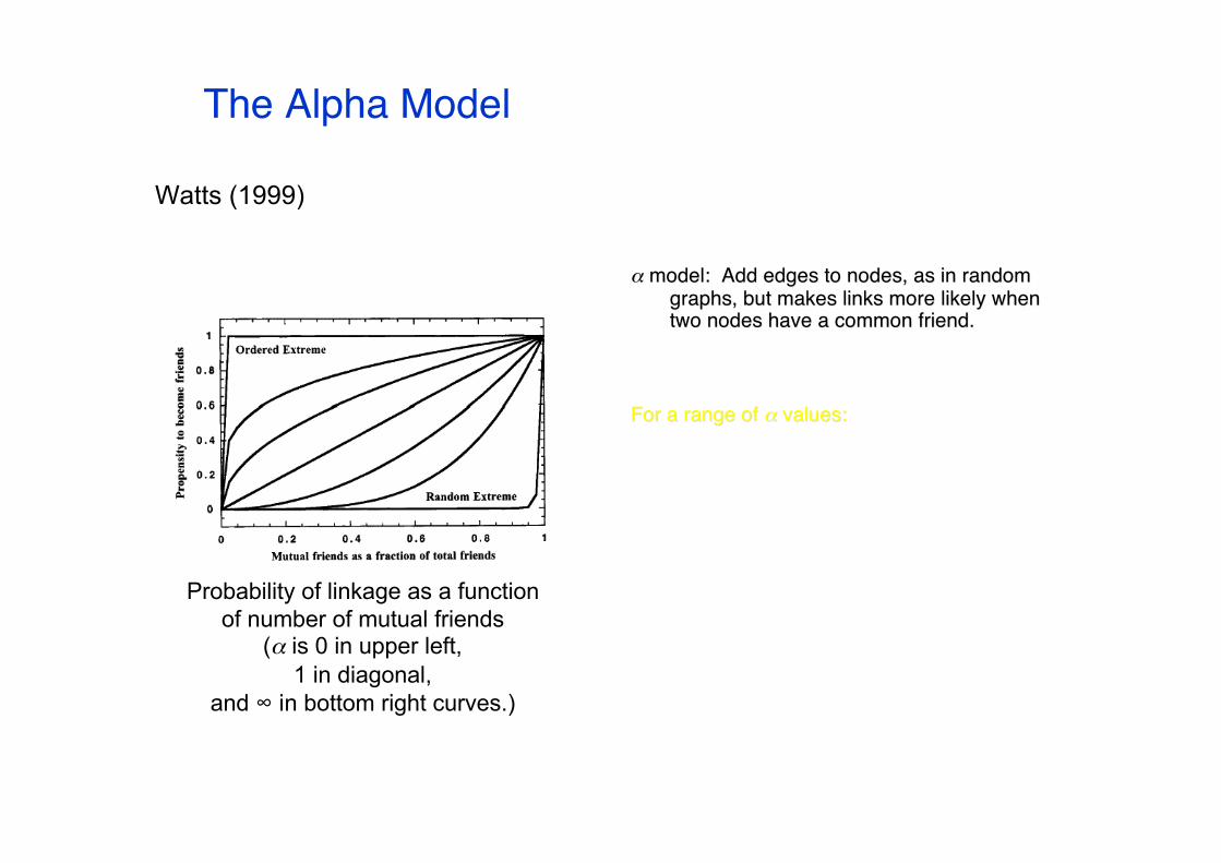
Watts (1999)
αα model: Add edges to nodes, as in random model: Add edges to nodes, as in randomgraphs, but makes links more likely whengraphs, but makes links more likely whentwo nodes have a common friend.two nodes have a common friend.
For a range of For a range of αα values: values:
The world is small (average path length isThe world is small (average path length isshort), andshort), and
Groups tend to form (high clusteringGroups tend to form (high clusteringcoefficient).coefficient).
Probability of linkage as a functionof number of mutual friends
(α is 0 in upper left,1 in diagonal,
and ∞ in bottom right curves.)

The Alpha Model
Watts (1999)
α
Clu
ster
ing
coef
ficie
nt /
Nor
mal
ized
pat
h le
ngth
Clustering coefficient (C) and average path length (L)
plotted against α
αα model: Add edges to nodes, as in random model: Add edges to nodes, as in randomgraphs, but makes links more likely whengraphs, but makes links more likely whentwo nodes have a common friend.two nodes have a common friend.
For a range of For a range of αα values: values:
The world is small (average path length isThe world is small (average path length isshort), andshort), and
Groups tend to form (high clusteringGroups tend to form (high clusteringcoefficient).coefficient).
The Beta Model
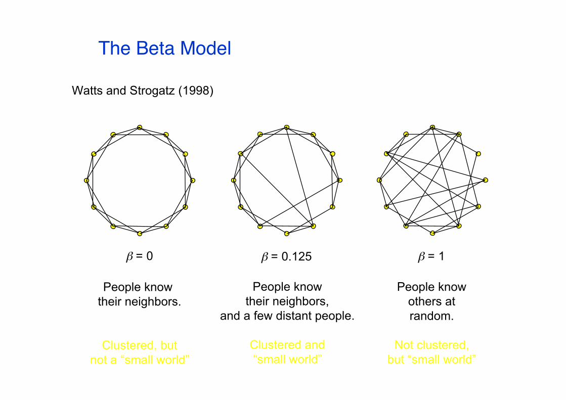
Watts and Strogatz (1998)
β = 0 β = 0.125 β = 1
People knowothers atrandom.
Not clustered,but “small world”
People knowtheir neighbors,
and a few distant people.
Clustered and“small world”
People know their neighbors.
Clustered, butnot a “small world”

The Beta Model
First five random links reduce the average pathFirst five random links reduce the average pathlength of the network by half, regardless of length of the network by half, regardless of NN!!
Both Both αα and and ββ models reproduce short-path results models reproduce short-path resultsof random graphs, but also allow for clustering.of random graphs, but also allow for clustering.
Small-world phenomena occur at thresholdSmall-world phenomena occur at thresholdbetween order and chaos.between order and chaos.
Watts and Strogatz (1998) NobuyukiHanaki
JonathanDonner
KentaroToyama
Clu
ster
ing
coef
ficie
nt /
Nor
mal
ized
pat
h le
ngth
Clustering coefficient (C) and average path length (L) plotted against β

Power LawsAlbert and Barabasi (1999)
Degree distribution of a random graph,N = 10,000 p = 0.0015 k = 15.
(Curve is a Poisson curve, for comparison.)
WhatWhat ʼ̓s the degree (number of edges) distributions the degree (number of edges) distributionover a graph, for real-world graphs?over a graph, for real-world graphs?
Random-graph model results in PoissonRandom-graph model results in Poissondistribution.distribution.
But, many real-world networks exhibit a But, many real-world networks exhibit a power-lawpower-lawdistribution.distribution.

Power LawsAlbert and Barabasi (1999)
Typical shape of a power-law distribution.
WhatWhat ʼ̓s the degree (number of edges) distributions the degree (number of edges) distributionover a graph, for real-world graphs?over a graph, for real-world graphs?
Random-graph model results in PoissonRandom-graph model results in Poissondistribution.distribution.
But, many real-world networks exhibit a But, many real-world networks exhibit a power-lawpower-lawdistribution.distribution.
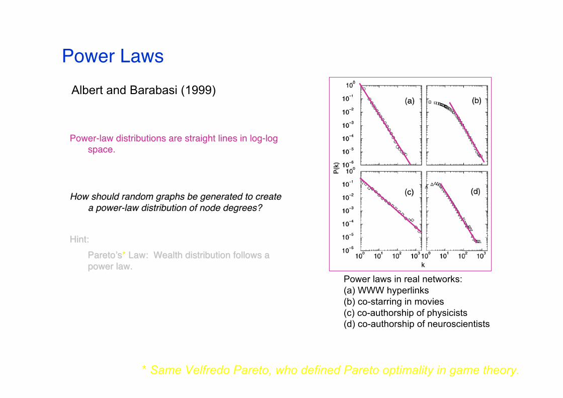
Power LawsAlbert and Barabasi (1999)
Power-law distributions are straight lines in log-logPower-law distributions are straight lines in log-logspace.space.
How should random graphs be generated to createHow should random graphs be generated to createa power-law distribution of node degrees?a power-law distribution of node degrees?
Hint:Hint:ParetoParetoʼ̓ss** Law: Wealth distribution follows a Law: Wealth distribution follows apower law.power law.
Power laws in real networks:(a) WWW hyperlinks(b) co-starring in movies(c) co-authorship of physicists(d) co-authorship of neuroscientists
* Same Velfredo Pareto, who defined Pareto optimality in game theory.
Power Laws
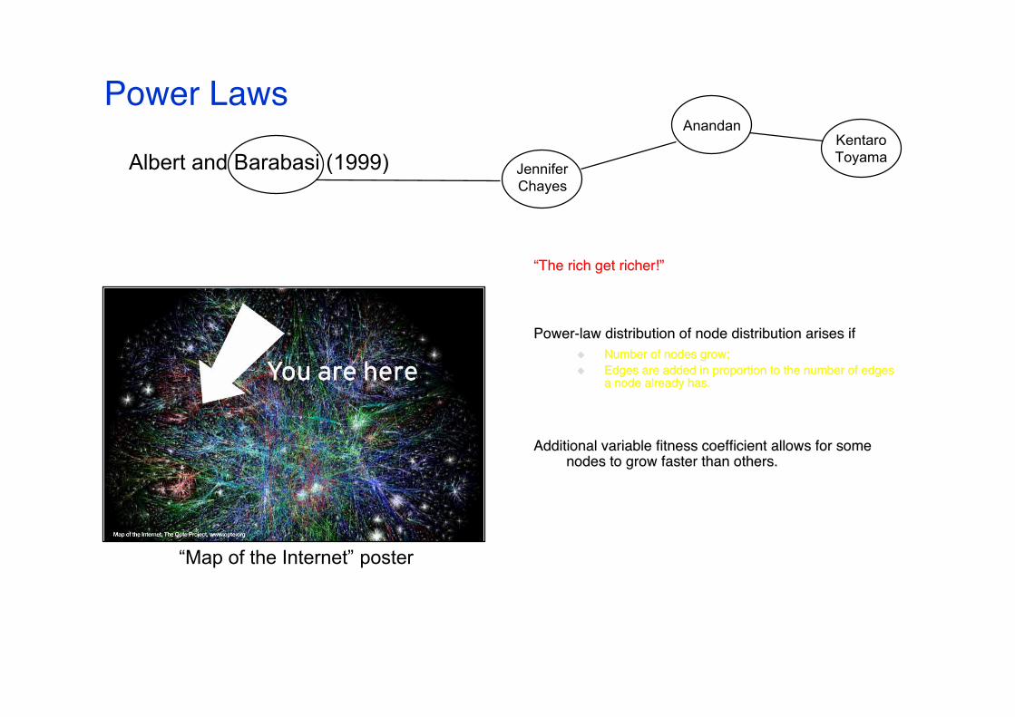
““The rich get richer!The rich get richer!””
Power-law distribution of node distribution arises ifPower-law distribution of node distribution arises if Number of nodes grow;Number of nodes grow; Edges are added in proportion to the number of edgesEdges are added in proportion to the number of edges
a node already has.a node already has.
Additional variable fitness coefficient allows for someAdditional variable fitness coefficient allows for somenodes to grow faster than others.nodes to grow faster than others.
Albert and Barabasi (1999) JenniferChayes
AnandanKentaroToyama
“Map of the Internet” poster
Searchable Networks
Just because a short path exists, doesnJust because a short path exists, doesn ʼ̓t meant meanyou can easily find it.you can easily find it.
You donYou don ʼ̓t know all of the people whom yourt know all of the people whom yourfriends know.friends know.
Under what conditions is a network Under what conditions is a network searchablesearchable??
Kleinberg (2000)
Searchable Networks
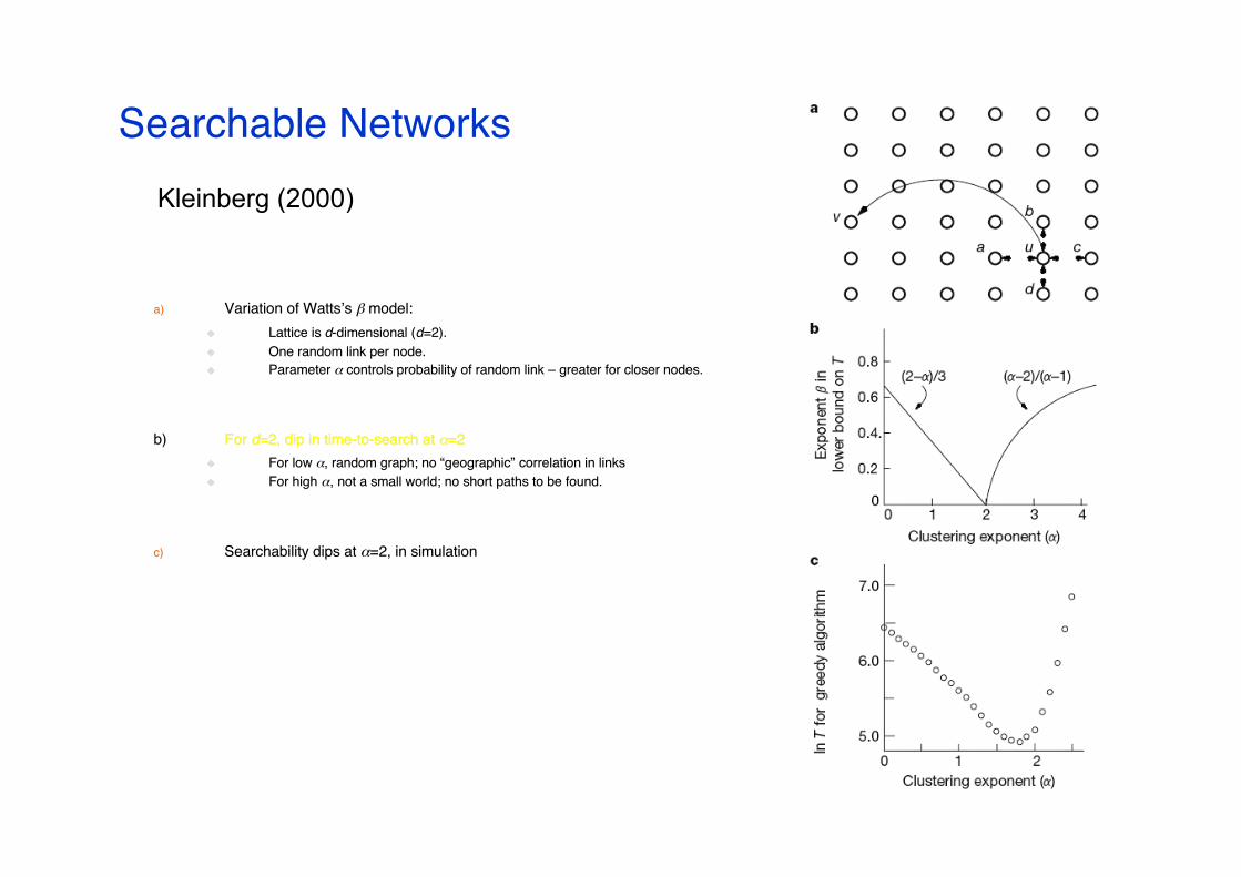
a)a) Variation of Variation of WattsWattsʼ̓s s ββ model: model: Lattice is Lattice is dd-dimensional (-dimensional (dd=2).=2). One random link per node.One random link per node. Parameter Parameter αα controls probability of random link controls probability of random link –– greater for closer nodes. greater for closer nodes.
b) b) For For dd=2, dip in time-to-search at =2, dip in time-to-search at αα=2=2 For low For low αα, random graph; no , random graph; no ““geographicgeographic”” correlation in links correlation in links For high For high αα, not a small world; no short paths to be found., not a small world; no short paths to be found.
c)c) Searchability Searchability dips at dips at αα=2, in simulation=2, in simulation
Kleinberg (2000)
Searchable Networks
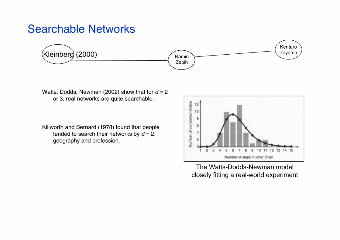
Watts, Watts, DoddsDodds, Newman (2002) show that for , Newman (2002) show that for dd = 2 = 2or 3, real networks are quite searchable.or 3, real networks are quite searchable.
Killworth Killworth and Bernard (1978) found that peopleand Bernard (1978) found that peopletended to search their networks by tended to search their networks by dd = 2: = 2:geography and profession.geography and profession.
Kleinberg (2000) RaminZabih
KentaroToyama
The Watts-Dodds-Newman modelclosely fitting a real-world experiment
References Aldous & Wilson, Graphs and Applications. AnIntroductory Approach, Springer, 2000. WWasserman & Faust, Social Network Analysis,Cambridge University Press, 2008.