Introduction to Numerical Methods

and Matlab Programming for Engineers

Todd Young and Martin J. Mohlenkamp

Department of Mathematics

Ohio University

Athens, OH 45701

youngt@ohio.edu

August 10, 2012

ii

Copyright c© 2008, 2009, 2011 Todd Young and Martin J. Mohlenkamp.Original edition 2004, by Todd Young. Permission is granted to copy, distributeand/or modify this document under the terms of the GNU Free Documenta-tion License, Version 1.3 or any later version published by the Free SoftwareFoundation; with no Invariant Sections, no Front-Cover Texts, and no Back-Cover Texts. A copy of the license is included in the section entitled “GNUFree Documentation License”.

Preface

These notes were developed by the first author in the process of teaching a course on appliednumerical methods for Civil Engineering majors during 2002-2004 and was modified toinclude Mechanical Engineering in 2005. The materials have been periodically updatedsince then and underwent a major revision by the second author in 2006-2007.

The main goals of these lectures are to introduce concepts of numerical methods and intro-duce Matlab in an Engineering framework. By this we do not mean that every problemis a “real life” engineering application, but more that the engineering way of thinking isemphasized throughout the discussion.

The philosophy of this book was formed over the course of many years. My father was aCivil Engineer and surveyor, and he introduced me to engineering ideas from an early age.At the University of Kentucky I took most of the basic Engineering courses while gettinga Bachelor’s degree in Mathematics. Immediately afterward I completed a M.S. degreein Engineering Mechanics at Kentucky. While working on my Ph.D. in Mathematics atGeorgia Tech I taught all of the introductory math courses for engineers. During myeducation, I observed that incorporation of computation in coursework had been extremelyunfocused and poor. For instance during my college career I had to learn 8 differentprogramming and markup languages on 4 different platforms plus numerous other softwareapplications. There was almost no technical help provided in the courses and I wastedinnumerable hours figuring out software on my own. A typical, but useless, inclusion ofsoftware has been (and still is in most calculus books) to set up a difficult ‘applied’ problemand then add the line “write a program to solve” or “use a computer algebra system tosolve”.

At Ohio University we have tried to take a much more disciplined and focused approach.The Russ College of Engineering and Technology decided that Matlab should be theprimary computational software for undergraduates. At about the same time members ofthe Mathematics Department proposed an 1804 project to bring Matlab into the calculussequence and provide access to the program at nearly all computers on campus, includingin the dorm rooms. The stated goal of this project was to make Matlab the universallanguage for computation on campus. That project was approved and implemented in the2001-2002 academic year.

In these lecture notes, instruction on using Matlab is dispersed through the material onnumerical methods. In these lectures details about how to use Matlab are detailed (butnot verbose) and explicit. To teach programming, students are usually given examples ofworking programs and are asked to make modifications.

iii

iv PREFACE

The lectures are designed to be used in a computer classroom, but could be used in alecture format with students doing computer exercises afterward. The lectures are dividedinto four Parts with a summary provided at the end of each Part. Throughout the textMatlab commands are preceded by the symbol >, which is the prompt in the commandwindow. Programs are surrounded by a box.

Todd Young, August 10, 2012

Contents

Preface iii

I Matlab and Solving Equations 1

Lecture 1. Vectors, Functions, and Plots in Matlab 2

Lecture 2. Matlab Programs 5

Lecture 3. Newton’s Method and Loops 8

Lecture 4. Controlling Error and Conditional Statements 11

Lecture 5. The Bisection Method and Locating Roots 14

Lecture 6. Secant Methods* 17

Lecture 7. Symbolic Computations 20

Review of Part I 23

II Linear Algebra 27

Lecture 8. Matrices and Matrix Operations in Matlab 28

Lecture 9. Introduction to Linear Systems 32

Lecture 10. Some Facts About Linear Systems 36

Lecture 11. Accuracy, Condition Numbers and Pivoting 39

Lecture 12. LU Decomposition 43

Lecture 13. Nonlinear Systems - Newton’s Method 46

Lecture 14. Eigenvalues and Eigenvectors 50

Lecture 15. An Application of Eigenvectors: Vibrational Modes 53

Lecture 16. Numerical Methods for Eigenvalues 56

Lecture 17. The QR Method* 60

v

vi CONTENTS

Lecture 18. Iterative solution of linear systems* 62

Review of Part II 63

III Functions and Data 67

Lecture 19. Polynomial and Spline Interpolation 68

Lecture 20. Least Squares Fitting: Noisy Data 72

Lecture 21. Integration: Left, Right and Trapezoid Rules 75

Lecture 22. Integration: Midpoint and Simpson’s Rules 79

Lecture 23. Plotting Functions of Two Variables 83

Lecture 24. Double Integrals for Rectangles 86

Lecture 25. Double Integrals for Non-rectangles 90

Lecture 26. Gaussian Quadrature* 93

Lecture 27. Numerical Differentiation 94

Lecture 28. The Main Sources of Error 97

Review of Part III 100

IV Differential Equations 105

Lecture 29. Reduction of Higher Order Equations to Systems 106

Lecture 30. Euler Methods 109

Lecture 31. Higher Order Methods 113

Lecture 32. Multi-step Methods* 116

Lecture 33. ODE Boundary Value Problems and Finite Differences 117

Lecture 34. Finite Difference Method – Nonlinear ODE 120

Lecture 35. Parabolic PDEs - Explicit Method 122

Lecture 36. Solution Instability for the Explicit Method 126

Lecture 37. Implicit Methods 129

Lecture 38. Insulated Boundary Conditions 132

Lecture 39. Finite Difference Method for Elliptic PDEs 136

CONTENTS vii

Lecture 40. Convection-Diffusion Equations 139

Lecture 41. Finite Elements 140

Lecture 42. Determining Internal Node Values 144

Review of Part IV 147

V Appendices 149

Lecture A. Sample Exams 150

Lecture B. Glossary of Matlab Commands 156

GNU Free Documentation License 162

1. APPLICABILITY AND DEFINITIONS . . . . . . . . . . . . . . . . . . . . . 162

2. VERBATIM COPYING . . . . . . . . . . . . . . . . . . . . . . . . . . . . . . 164

3. COPYING IN QUANTITY . . . . . . . . . . . . . . . . . . . . . . . . . . . . 165

4. MODIFICATIONS . . . . . . . . . . . . . . . . . . . . . . . . . . . . . . . . . 165

5. COMBINING DOCUMENTS . . . . . . . . . . . . . . . . . . . . . . . . . . . 167

6. COLLECTIONS OF DOCUMENTS . . . . . . . . . . . . . . . . . . . . . . . 168

7. AGGREGATION WITH INDEPENDENT WORKS . . . . . . . . . . . . . . 168

8. TRANSLATION . . . . . . . . . . . . . . . . . . . . . . . . . . . . . . . . . . 169

9. TERMINATION . . . . . . . . . . . . . . . . . . . . . . . . . . . . . . . . . . 169

10. FUTURE REVISIONS OF THIS LICENSE . . . . . . . . . . . . . . . . . . 170

11. RELICENSING . . . . . . . . . . . . . . . . . . . . . . . . . . . . . . . . . . 170

ADDENDUM: How to use this License for your documents . . . . . . . . . . . . 171

viii CONTENTS

Part I

Matlab and Solving Equations

c©Copyright, Todd Young and Martin Mohlenkamp, Mathematics Department, Ohio University, 2007

Lecture 1

Vectors, Functions, and Plots in Matlab

In this book > will indicate commands to be entered in the command window. You do not actuallytype the command prompt > .

Entering vectors

In Matlab, the basic objects are matrices, i.e. arrays of numbers. Vectors can be thought of asspecial matrices. A row vector is recorded as a 1 × n matrix and a column vector is recorded asa m × 1 matrix. To enter a row vector in Matlab, type the following at the prompt ( > ) in thecommand window:> v = [0 1 2 3]

and press enter. Matlab will print out the row vector. To enter a column vector type:> u = [9; 10; 11; 12; 13]

You can access an entry in a vector with> u(2)

and change the value of that entry with> u(2)=47

You can extract a slice out of a vector with> u(2:4)

You can change a row vector into a column vector, and vice versa easily in Matlab using:> w = v’

(This is called transposing the vector and we call ’ the transpose operator.) There are also usefulshortcuts to make vectors such as:> x = -1:.1:1

and> y = linspace(0,1,11)

Plotting Data

Consider the following table, obtained from experiments on the viscosity of a liquid.1 We can enter

T (C) 5 20 30 50 55µ 0.08 0.015 0.009 0.006 0.0055

this data into Matlab with the following commands entered in the command window:> x = [ 5 20 30 50 55 ]

1Adapted from Ayyup & McCuen 1996, p.174.

2

3

> y = [ 0.08 0.015 0.009 0.006 0.0055]

Entering the name of the variable retrieves its current values. For instance:> x

> y

We can plot data in the form of vectors using the plot command:> plot(x,y)

This will produce a graph with the data points connected by lines. If you would prefer that thedata points be represented by symbols you can do so. For instance:> plot(x,y,’*’)

> plot(x,y,’o’)

> plot(x,y,’.’)

Data as a Representation of a Function

A major theme in this course is that often we are interested in a certain function y = f(x), butthe only information we have about this function is a discrete set of data (xi, yi). Plotting thedata, as we did above, can be thought of envisioning the function using just the data. We will findlater that we can also do other things with the function, like differentiating and integrating, justusing the available data. Numerical methods, the topic of this course, means doing mathematics bycomputer. Since a computer can only store a finite amount of information, we will almost alwaysbe working with a finite, discrete set of values of the function (data), rather than a formula for thefunction.

Built-in Functions

If we wish to deal with formulas for functions, Matlab contains a number of built-in functions,including all the usual functions, such as sin( ), exp( ), etc.. The meaning of most of these isclear. The dependent variable (input) always goes in parentheses in Matlab. For instance:> sin(pi)

should return the value of sinπ, which is of course 0 and> exp(0)

will return e0 which is 1. More importantly, the built-in functions can operate not only on singlenumbers but on vectors. For example:> x = linspace(0,2*pi,40)

> y = sin(x)

> plot(x,y)

will return a plot of sinx on the interval [0, 2π]

Some of the built-in functions in Matlab include: cos( ), tan( ), sinh( ), cosh( ), log( )

(natural logarithm), log10( ) (log base 10), asin( ) (inverse sine), acos( ), atan( ). To findout more about a function, use the help command; try> help plot

User-Defined Inline Functions

If we wish to deal with a function that is a combination of the built-in functions, Matlab has acouple of ways for the user to define functions. One that we will use a lot is the inline function, which

4 LECTURE 1. VECTORS, FUNCTIONS, AND PLOTS IN MATLAB

is a way to define a function in the command window. The following is a typical inline function:> f = inline(’2*x.^2 - 3*x + 1’,’x’)

This produces the function f(x) = 2x2 − 3x+ 1. To obtain a single value of this function enter:> f(2.23572)

Just as for built-in functions, the function f as we defined it can operate not only on single numbersbut on vectors. Try the following:> x = -2:.2:2

> y = f(x)

This is an example of vectorization, i.e. putting several numbers into a vector and treating thevector all at once, rather than one component at a time, and is one of the strengths of Mat-

lab. The reason f(x) works when x is a vector is because we represented x2 by x.^2. The .

turns the exponent operator ^ into entry-wise exponentiation, so that [-2 -1.8 -1.6].^2 means[(−2)2, (−1.8)2, (−1.6)2] and yields [4 3.24 2.56]. In contrast, [-2 -1.8 -1.6]^2 means the ma-trix product [−2,−1.8,−1.6][−2,−1.8,−1.6] and yields only an error. The . is needed in .^, .*,and ./. It is not needed when you * or / by a scalar or for +.

The results can be plotted using the plot command, just as for data:> plot(x,y)

Notice that before plotting the function, we in effect converted it into data. Plotting on any machinealways requires this step.

Exercises

1.1 Find a table of data in an engineering textbook. Input it as vectors and plot it. Use the inserticon to label the axes and add a title to your graph. Turn in the graph. Indicate what thedata is and where it came from.

1.2 Make an inline function g(x) = x + cos(x5). Plot it using vectors x = -5:.1:5; andy = g(x);. What is wrong with this graph? Find a way to make it look more like thegraph of g(x) should. Turn in both plots.

Lecture 2

Matlab Programs

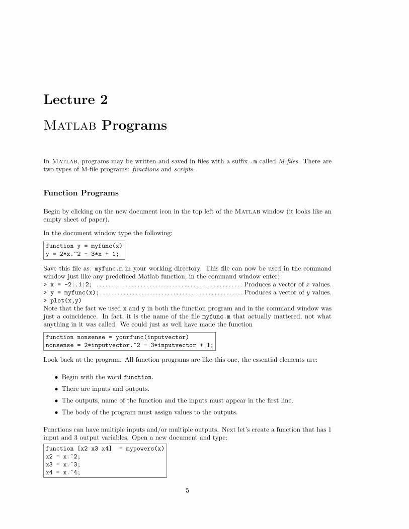
In Matlab, programs may be written and saved in files with a suffix .m called M-files. There aretwo types of M-file programs: functions and scripts.

Function Programs

Begin by clicking on the new document icon in the top left of the Matlab window (it looks like anempty sheet of paper).

In the document window type the following:

function y = myfunc(x)

y = 2*x.^2 - 3*x + 1;

Save this file as: myfunc.m in your working directory. This file can now be used in the commandwindow just like any predefined Matlab function; in the command window enter:> x = -2:.1:2; . . . . . . . . . . . . . . . . . . . . . . . . . . . . . . . . . . . . . . . . . . . . . . . . . . Produces a vector of x values.> y = myfunc(x); . . . . . . . . . . . . . . . . . . . . . . . . . . . . . . . . . . . . . . . . . . . . . . . . Produces a vector of y values.> plot(x,y)

Note that the fact we used x and y in both the function program and in the command window wasjust a coincidence. In fact, it is the name of the file myfunc.m that actually mattered, not whatanything in it was called. We could just as well have made the function

function nonsense = yourfunc(inputvector)

nonsense = 2*inputvector.^2 - 3*inputvector + 1;

Look back at the program. All function programs are like this one, the essential elements are:

• Begin with the word function.

• There are inputs and outputs.

• The outputs, name of the function and the inputs must appear in the first line.

• The body of the program must assign values to the outputs.

Functions can have multiple inputs and/or multiple outputs. Next let’s create a function that has 1input and 3 output variables. Open a new document and type:

function [x2 x3 x4] = mypowers(x)

x2 = x.^2;

x3 = x.^3;

x4 = x.^4;

5

6 LECTURE 2. MATLAB PROGRAMS

Save this file as mypowers.m. In the command window, we can use the results of the program tomake graphs:> x = -1:.1:1

> [x2 x3 x4] = mypowers(x);

> plot(x,x,’black’,x,x2,’blue’,x,x3,’green’,x,x4,’red’)

Script Programs

Matlab uses a second type of program that differs from a function program in several ways, namely:

• There are no inputs and outputs.

• A script program may use and change variables in the current workspace (the variables usedby the command window.)

Below is a script program that accomplishes the same thing as the function program plus thecommands in the previous section:

x2 = x.^2;

x3 = x.^3;

x4 = x.^4;

plot(x,x,’black’,x,x2,’blue’,x,x3,’green’,x,x4,’red’)

Type this program into a new document and save it as mygraphs.m. In the command window enter:> x = -1:.1:1;

> mygraphs

Note that the program used the variable x in its calculations, even though x was defined in thecommand window, not in the program.

Many people use script programs for routine calculations that would require typing more than onecommand in the command window. They do this because correcting mistakes is easier in a programthan in the command window.

Program Comments

For programs that have more than a couple of lines it is important to include comments. Commentsallow other people to know what your program does and they also remind yourself what yourprogram does if you set it aside and come back to it later. It is best to include comments not onlyat the top of a program, but also with each section. In Matlab anything that comes in a line aftera % is a comment.

For a function program, the comments should at least give the purpose, inputs, and outputs. Aproperly commented version of the function with which we started this section is:

function y = myfunc(x)

% Computes the function 2x^2 -3x +1

% Input: x -- a number or vector; for a vector the computation is elementwise

% Output: y -- a number or vector of the same size as x

y = 2*x.^2 - 3*x + 1;

7

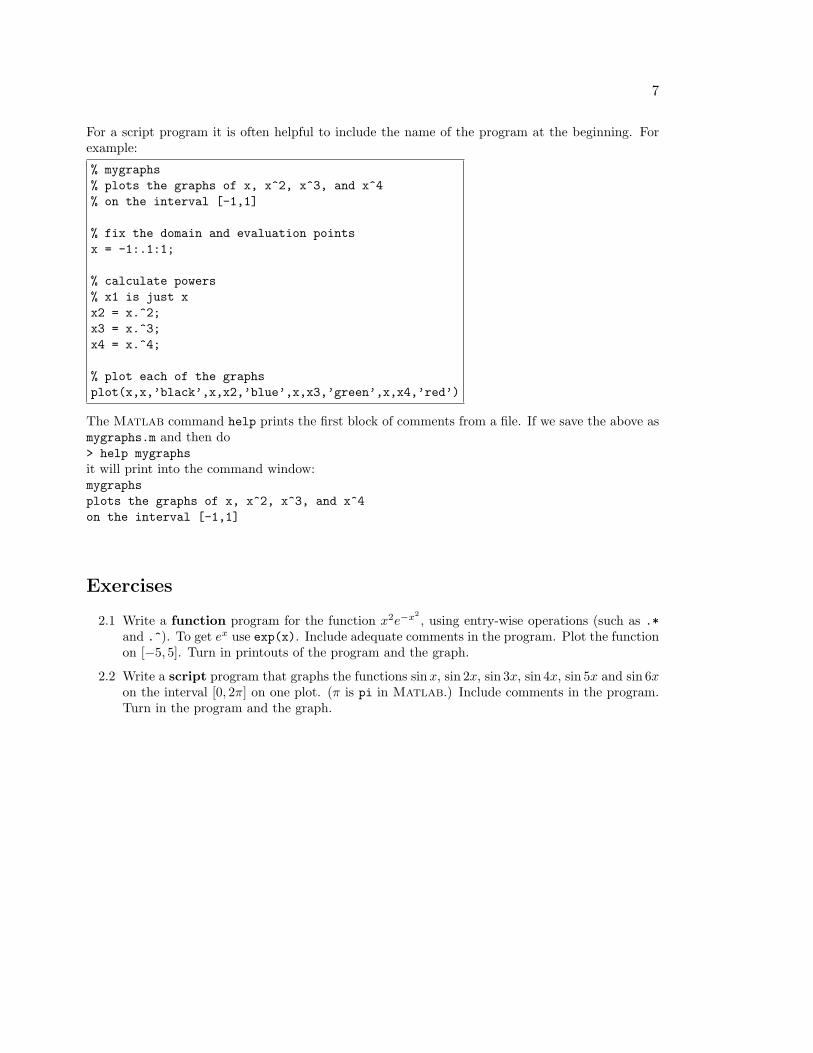
For a script program it is often helpful to include the name of the program at the beginning. Forexample:

% mygraphs

% plots the graphs of x, x^2, x^3, and x^4

% on the interval [-1,1]

% fix the domain and evaluation points

x = -1:.1:1;

% calculate powers

% x1 is just x

x2 = x.^2;

x3 = x.^3;

x4 = x.^4;

% plot each of the graphs

plot(x,x,’black’,x,x2,’blue’,x,x3,’green’,x,x4,’red’)

The Matlab command help prints the first block of comments from a file. If we save the above asmygraphs.m and then do> help mygraphs

it will print into the command window:mygraphs

plots the graphs of x, x^2, x^3, and x^4

on the interval [-1,1]

Exercises

2.1 Write a function program for the function x2e−x2

, using entry-wise operations (such as .*and .^). To get ex use exp(x). Include adequate comments in the program. Plot the functionon [−5, 5]. Turn in printouts of the program and the graph.

2.2 Write a script program that graphs the functions sinx, sin 2x, sin 3x, sin 4x, sin 5x and sin 6xon the interval [0, 2π] on one plot. (π is pi in Matlab.) Include comments in the program.Turn in the program and the graph.

Lecture 3

Newton’s Method and Loops

Solving equations numerically

For the next few lectures we will focus on the problem of solving an equation:

f(x) = 0. (3.1)

As you learned in calculus, the final step in many optimization problems is to solve an equation ofthis form where f is the derivative of a function, F , that you want to maximize or minimize. In realengineering problems the function you wish to optimize can come from a large variety of sources,including formulas, solutions of differential equations, experiments, or simulations.

Newton iterations

We will denote an actual solution of equation (3.1) by x∗. There are three methods which you mayhave discussed in Calculus: the bisection method, the secant method and Newton’s method. Allthree depend on beginning close (in some sense) to an actual solution x∗.

Recall Newton’s method. You should know that the basis for Newton’s method is approximation ofa function by it linearization at a point, i.e.

f(x) ≈ f(x0) + f ′(x0)(x− x0). (3.2)

Since we wish to find x so that f(x) = 0, set the left hand side (f(x)) of this approximation equalto 0 and solve for x to obtain:

x ≈ x0 −f(x0)

f ′(x0). (3.3)

We begin the method with the initial guess x0, which we hope is fairly close to x∗. Then we definea sequence of points x0, x1, x2, x3, . . . from the formula:

xi+1 = xi −f(xi)

f ′(xi), (3.4)

which comes from (3.3). If f(x) is reasonably well-behaved near x∗ and x0 is close enough to x∗,then it is a fact that the sequence will converge to x∗ and will do it very quickly.

The loop: for ... end

In order to do Newton’s method, we need to repeat the calculation in (3.4) a number of times. Thisis accomplished in a program using a loop, which means a section of a program which is repeated.

8

9

The simplest way to accomplish this is to count the number of times through. In Matlab, afor ... end statement makes a loop as in the following simple function program:

function S = mysum(n)

% gives the sum of the first n integers

S = 0; % start at zero

% The loop:

for i = 1:n % do n times

S = S + i; % add the current integer

end % end of the loop

Call this function in the command window as:> mysum(100)

The result will be the sum of the first 100 integers. All for ... end loops have the same format, itbegins with for, followed by an index (i) and a range of numbers (1:n). Then come the commandsthat are to be repeated. Last comes the end command.

Loops are one of the main ways that computers are made to do calculations that humans cannot.Any calculation that involves a repeated process is easily done by a loop.

Now let’s do a program that does n steps (iterations) of Newton’s method. We will need to inputthe function, its derivative, the initial guess, and the number of steps. The output will be the finalvalue of x, i.e. xn. If we are only interested in the final approximation, not the intermediate steps,which is usually the case in the real world, then we can use a single variable x in the program andchange it at each step:

function x = mynewton(f,f1,x0,n)

% Solves f(x) = 0 by doing n steps of Newton’s method starting at x0.

% Inputs: f -- the function, input as an inline

% f1 -- it’s derivative, input as an inline

% x0 -- starting guess, a number

% n -- the number of steps to do

% Output: x -- the approximate solution

format long % prints more digits

format compact % makes the output more compact

x = x0; % set x equal to the initial guess x0

for i = 1:n % Do n times

x = x - f(x)/f1(x) % Newton’s formula, prints x too

end

In the command window define an inline function: f(x) = x3 − 5 i.e.> f = inline(’x^3 - 5’)

and define f1 to be its derivative, i.e.> f1 = inline(’3*x^2’).

Then run mynewton on this function. By trial and error, what is the lowest value of n for which theprogram converges (stops changing). By simple algebra, the true root of this function is 3

√5. How

close is the program’s answer to the true value?

Convergence

Newton’s method converges rapidly when f ′(x∗) is nonzero and finite, and x0 is close enough to x∗

that the linear approximation (3.2) is valid. Let us take a look at what can go wrong.

10 LECTURE 3. NEWTON’S METHOD AND LOOPS

For f(x) = x1/3 we have x∗ = 0 but f ′(x∗) = ∞. If you try> f = inline(’x^(1/3)’)

> f1 = inline(’(1/3)*x^(-2/3)’)

> x = mynewton(f,f1,0.1,10)

then x explodes.

For f(x) = x2 we have x∗ = 0 but f ′(x∗) = 0. If you try> f = inline(’x^2’)

> f1 = inline(’2*x’)

> x = mynewton(f,f1,1,10)

then x does converge to 0, but not that rapidly.

If x0 is not close enough to x∗ that the linear approximation (3.2) is valid, then the iteration (3.4)gives some x1 that may or may not be any better than x0. If we keep iterating, then either

• xn will eventually get close to x∗ and the method will then converge (rapidly), or

• the iterations will not approach x∗.

Exercises

3.1 Enter: format long. Use mynewton on the function f(x) = x5− 7, with x0 = 2. By trial anderror, what is the lowest value of n for which the program converges (stops changing). Howclose is the answer to the true value? Plug the program’s answer into f(x); is the value zero?

3.2 Suppose a ball is dropped from a height of 2 meters onto a hard surface and the coefficient ofrestitution of the collision is .9 (see Wikipedia for an explanation). Write a script program tocalculate the distance traveled by the ball after n bounces. Include lots of comments. Enter:format long. By trial and error approximate how large n must be so that total distancestops changing. Turn in the program and a brief summary of the results.

3.3 For f(x) = x3 − 4, perform 3 iterations of Newton’s method with starting point x0 = 2. (Onpaper, but use a calculator.) Calculate the solution (x∗ = 41/3) on a calculator and find theerrors and percentage errors of x0, x1, x2 and x3. Put the results in a table.

Lecture 4

Controlling Error and ConditionalStatements

Measuring error and the Residual

If we are trying to find a numerical solution of an equation f(x) = 0, then there are a few differentways we can measure the error of our approximation. The most direct way to measure the errorwould be as:

Error at step n = en = xn − x∗

where xn is the n-th approximation and x∗ is the true value. However, we usually do not know thevalue of x∗, or we wouldn’t be trying to approximate it. This makes it impossible to know the errordirectly, and so we must be more clever.

One possible strategy, that often works, is to run a program until the approximation xn stopschanging. The problem with this is that sometimes doesn’t work. Just because the program stopchanging does not necessarily mean that xn is close to the true solution.

For Newton’s method we have the following principle: At each step the number of significantdigits roughly doubles. While this is an important statement about the error (since it meansNewton’s method converges really quickly), it is somewhat hard to use in a program.

Rather than measure how close xn is to x∗, in this and many other situations it is much more practicalto measure how close the equation is to being satisfied, in other words, how close yn = f(xn) is to0. We will use the quantity rn = f(xn)− 0, called the residual, in many different situations. Mostof the time we only care about the size of rn, so we look at |rn| = |f(xn)|.

The if ... end statement

If we have a certain tolerance for |rn| = |f(xn)|, then we can incorporate that into our Newtonmethod program using an if ... end statement:

11

12 LECTURE 4. CONTROLLING ERROR AND CONDITIONAL STATEMENTS

function x = mynewton(f,f1,x0,n,tol)

% Solves f(x) = 0 by doing n steps of Newton’s method starting at x0.

% Inputs: f -- the function, input as an inline

% f1 -- it’s derivative, input as an inline

% x0 -- starting guess, a number

% tol -- desired tolerance, prints a warning if |f(x)|>tol

% Output: x -- the approximate solution

x = x0; % set x equal to the initial guess x0

for i = 1:n % Do n times

x = x - f(x)/f1(x) % Newton’s formula

end

r = abs(f(x))

if r > tol

warning(’The desired accuracy was not attained’)

end

In this program if checks if abs(y) > tol is true or not. If it is true then it does everythingbetween there and end. If not true, then it skips ahead to end.

In the command window define the function> f = inline(’x^3-5’,’x’)

and its derivative> f1 = inline(’3*x^2’,’x’).

Then use the program with n = 5, tol = .01, and x0 = 2. Next, change tol to 10−10 and repeat.

The loop: while ... end

While the previous program will tell us if it worked or not, we still have to input n, the number ofsteps to take. Even for a well-behaved problem, if we make n too small then the tolerance will notbe attained and we will have to go back and increase it, or, if we make n too big, then the programwill take more steps than necessary.

One way to control the number of steps taken is to iterate until the residual |rn| = |f(x)| = |y| issmall enough. In Matlab this is easily accomplished with a while ... end loop.

function x = mynewtontol(f,f1,x0,tol)

x = x0; % set x equal to the initial guess x0

y = f(x);

while abs(y) > tol % Do until the tolerence is reached.

x = x - y/f1(x) % Newton’s formula

y = f(x)

end

The statement while ... end is a loop, similar to for ... end, but instead of going through theloop a fixed number of times it keeps going as long as the statement abs(y) > tol is true.

One obvious drawback of the program is that abs(y) might never get smaller than tol. If thishappens, the program would continue to run over and over until we stop it. Try this by setting thetolerance to a really small number:> tol = 10^(-100)

then run the program again for f(x) = x3 − 5.

You can use Ctrl-c to stop the program when it’s stuck.

13

One way to avoid an infinite loop is add a counter variable, say i and a maximum number ofiterations to the programs.

Using the while statement, this can be accomplished as:

function x = mynewtontol(f,f1,x0,tol)

x = x0; i=0; % set x equal to the initial guess x0. set counter to zero

y = f(x);

while abs(y) > tol & i < 1000 % Do until the tolerence is reached or max iter.

x = x - y/f1(x) % Newton’s formula

y = f(x)

i = i+1;

end

Exercises

4.1 In Calculus we learn that a geometric series has an exact sum:

∞∑

i=0

ri =1

1− r

provided that |r| < 1. For instance, if r = .5 then the sum is exactly 2. Below is a scriptprogram that lacks one line as written. Put in the missing command and then use the programto verify the result above.

How many steps does it take? How close is the answer to 2? Change r = .5 to r=.9. Howmany steps does it take now? How accurate is the answer? Try this also for r = .99, .999, .9999.Report your results. At what point does the program’s output diverge from the know exact

answer?

format long

r = .5;

Snew = 0; % start sum at 0

Sold = -1; % set Sold to trick while the first time

i = 0; % count iterations

while Snew > Sold % is the sum still changing?

Sold = Snew; % save previous value to compare to

Snew = Snew + r^i;

i=i+1;

Snew % prints the final value.

i % prints the # of iterations.

4.2 Modify your program from exercise 3.2 to compute the total distance traveled by the ballwhile its bounces are at least 1 centimeter high. Use a while loop to decide when to stopsumming; do not use a for loop or trial and error. Turn in your modified program and a briefsummary of the results.

Lecture 5

The Bisection Method and LocatingRoots

Bisecting and the if ... else ... end statement

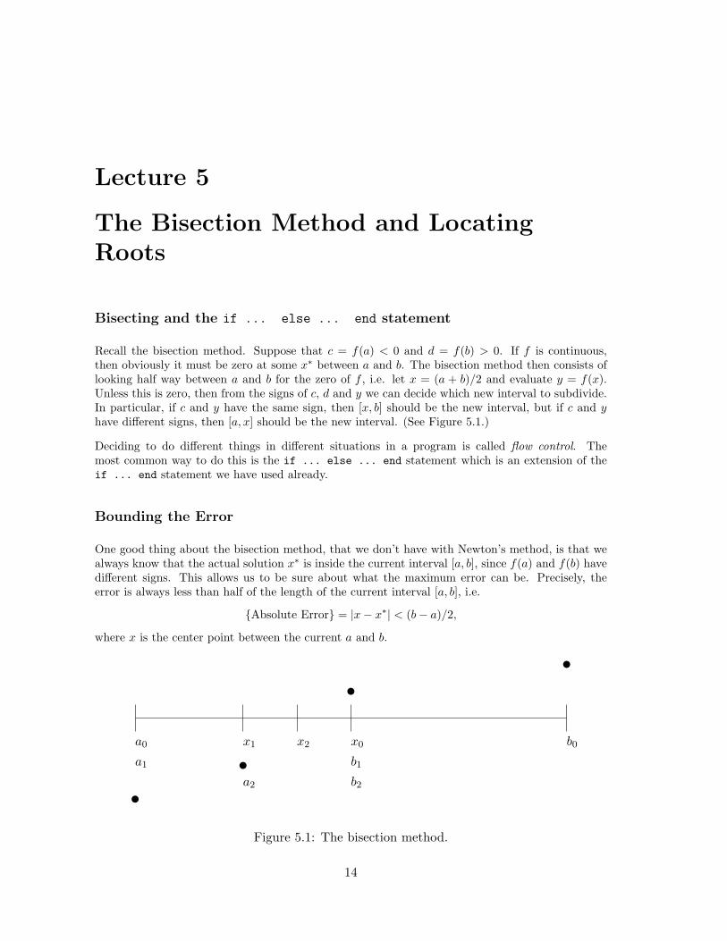
Recall the bisection method. Suppose that c = f(a) < 0 and d = f(b) > 0. If f is continuous,then obviously it must be zero at some x∗ between a and b. The bisection method then consists oflooking half way between a and b for the zero of f , i.e. let x = (a + b)/2 and evaluate y = f(x).Unless this is zero, then from the signs of c, d and y we can decide which new interval to subdivide.In particular, if c and y have the same sign, then [x, b] should be the new interval, but if c and yhave different signs, then [a, x] should be the new interval. (See Figure 5.1.)

Deciding to do different things in different situations in a program is called flow control. Themost common way to do this is the if ... else ... end statement which is an extension of theif ... end statement we have used already.

Bounding the Error

One good thing about the bisection method, that we don’t have with Newton’s method, is that wealways know that the actual solution x∗ is inside the current interval [a, b], since f(a) and f(b) havedifferent signs. This allows us to be sure about what the maximum error can be. Precisely, theerror is always less than half of the length of the current interval [a, b], i.e.

Absolute Error = |x− x∗| < (b− a)/2,

where x is the center point between the current a and b.

x0x1 x2a0 b0

a1 b1

a2 b2u

u

u

u

Figure 5.1: The bisection method.

14

15

The following function program (also available on the webpage) does n iterations of the bisectionmethod and returns not only the final value, but also the maximum possible error:

function [x e] = mybisect(f,a,b,n)

% function [x e] = mybisect(f,a,b,n)

% Does n iterations of the bisection method for a function f

% Inputs: f -- an inline function

% a,b -- left and right edges of the interval

% n -- the number of bisections to do.

% Outputs: x -- the estimated solution of f(x) = 0

% e -- an upper bound on the error

format long

c = f(a); d = f(b);

if c*d > 0.0

error(’Function has same sign at both endpoints.’)

end

disp(’ x y’)

for i = 1:n

x = (a + b)/2;

y = f(x);

disp([ x y])

if y == 0.0 % solved the equation exactly

e = 0;

break % jumps out of the for loop

end

if c*y < 0

b=x;

else

a=x;

end

end

e = (b-a)/2;

Another important aspect of bisection is that it always works. We saw that Newton’s method canfail to converge to x∗ if x0 is not close enough to x∗. In contrast, the current interval [a, b] inbisection will always get decreased by a factor of 2 at each step and so it will always eventuallyshrink down as small as you want it.

Locating a root

The bisection method and Newton’s method are both used to obtain closer and closer approximationsof a solution, but both require starting places. The bisection method requires two points a and bthat have a root between them, and Newton’s method requires one point x0 which is reasonablyclose to a root. How do you come up with these starting points? It depends. If you are solving anequation once, then the best thing to do first is to just graph it. From an accurate graph you cansee approximately where the graph crosses zero.

There are other situations where you are not just solving an equation once, but have to solve the sameequation many times, but with different coefficients. This happens often when you are developingsoftware for a specific application. In this situation the first thing you want to take advantage of isthe natural domain of the problem, i.e. on what interval is a solution physically reasonable. If that

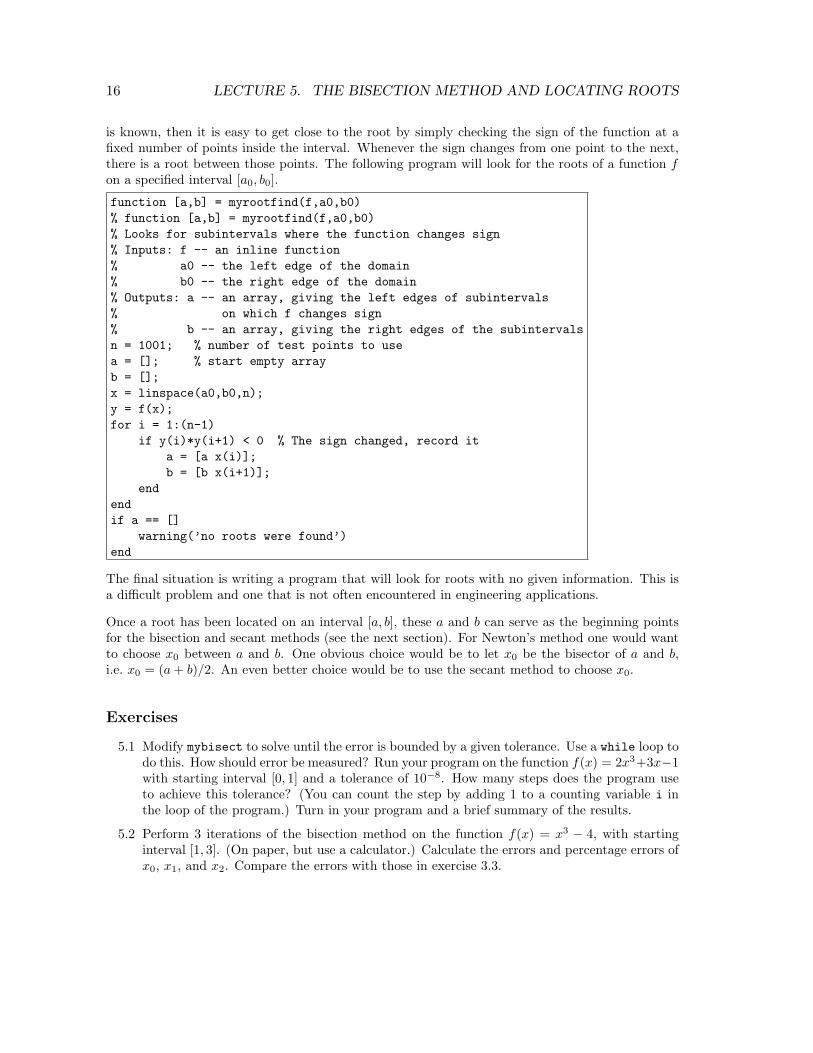
16 LECTURE 5. THE BISECTION METHOD AND LOCATING ROOTS

is known, then it is easy to get close to the root by simply checking the sign of the function at afixed number of points inside the interval. Whenever the sign changes from one point to the next,there is a root between those points. The following program will look for the roots of a function fon a specified interval [a0, b0].

function [a,b] = myrootfind(f,a0,b0)

% function [a,b] = myrootfind(f,a0,b0)

% Looks for subintervals where the function changes sign

% Inputs: f -- an inline function

% a0 -- the left edge of the domain

% b0 -- the right edge of the domain

% Outputs: a -- an array, giving the left edges of subintervals

% on which f changes sign

% b -- an array, giving the right edges of the subintervals

n = 1001; % number of test points to use

a = []; % start empty array

b = [];

x = linspace(a0,b0,n);

y = f(x);

for i = 1:(n-1)

if y(i)*y(i+1) < 0 % The sign changed, record it

a = [a x(i)];

b = [b x(i+1)];

end

end

if a == []

warning(’no roots were found’)

end

The final situation is writing a program that will look for roots with no given information. This isa difficult problem and one that is not often encountered in engineering applications.

Once a root has been located on an interval [a, b], these a and b can serve as the beginning pointsfor the bisection and secant methods (see the next section). For Newton’s method one would wantto choose x0 between a and b. One obvious choice would be to let x0 be the bisector of a and b,i.e. x0 = (a+ b)/2. An even better choice would be to use the secant method to choose x0.

Exercises

5.1 Modify mybisect to solve until the error is bounded by a given tolerance. Use a while loop todo this. How should error be measured? Run your program on the function f(x) = 2x3+3x−1with starting interval [0, 1] and a tolerance of 10−8. How many steps does the program useto achieve this tolerance? (You can count the step by adding 1 to a counting variable i inthe loop of the program.) Turn in your program and a brief summary of the results.

5.2 Perform 3 iterations of the bisection method on the function f(x) = x3 − 4, with startinginterval [1, 3]. (On paper, but use a calculator.) Calculate the errors and percentage errors ofx0, x1, and x2. Compare the errors with those in exercise 3.3.

Lecture 6

Secant Methods*

In this lecture we introduce two additional methods to find numerical solutions of the equationf(x) = 0. Both of these methods are based on approximating the function by secant lines just asNewton’s method was based on approximating the function by tangent lines.

The Secant Method

The secant method requires two initial points x0 and x1 which are both reasonably close to thesolution x∗. Preferably the signs of y0 = f(x0) and y1 = f(x1) should be different. Once x0 and x1

are determined the method proceeds by the following formula:

xi+1 = xi −xi − xi−1

yi − yi−1yi (6.1)

Example: Suppose f(x) = x4 − 5 for which the true solution is x∗ = 4√5. Plotting this function

reveals that the solution is at about 1.25. If we let x0 = 1 and x1 = 2 then we know that the rootis in between x0 and x1. Next we have that y0 = f(1) = −4 and y1 = f(2) = 11. We may thencalculate x2 from the formula (6.1):

x2 = 2− 2− 1

11− (−4)11 =

19

15≈ 1.2666....

Pluggin x2 = 19/15 into f(x) we obtain y2 = f(19/15) ≈ −2.425758.... In the next step we woulduse x1 = 2 and x2 = 19/15 in the formula (6.1) to find x3 and so on.

Below is a program for the secant method. Notice that it requires two input guesses x0 and x1, butit does not require the derivative to be input.

figure yet to be drawn, alas

Figure 6.1: The secant method.

17

18 LECTURE 6. SECANT METHODS*

function x = mysecant(f,x0,x1,n)

format long % prints more digits

format compact % makes the output more compact

% Solves f(x) = 0 by doing n steps of the secant method starting with x0 and x1.

% Inputs: f -- the function, input as an inline function

% x0 -- starting guess, a number

% x1 -- second starting geuss

% n -- the number of steps to do

% Output: x -- the approximate solution

y0 = f(x0);

y1 = f(x1);

for i = 1:n % Do n times

x = x1 - (x1-x0)*y1/(y1-y0) % secant formula.

y=f(x) % y value at the new approximate solution.

% Move numbers to get ready for the next step

x0=x1;

y0=y1;

x1=x;

y1=y;

end

The Regula Falsi Method

The Regula Falsi method is somewhat a combination of the secant method and bisection method.The idea is to use secant lines to approximate f(x), but choose how to update using the sign off(xn).

Just as in the bisection method, we begin with a and b for which f(a) and f(b) have different signs.Then let:

x = b− b− a

f(b)− f(a)f(b).

Next check the sign of f(x). If it is the same as the sign of f(a) then x becomes the new a. Otherwiselet b = x.

Convergence

If we can begin with a good choice x0, then Newton’s method will converge to x∗ rapidly. The secantmethod is a little slower than Newton’s method and the Regula Falsi method is slightly slower thanthat. Both however are still much faster than the bisection method.

If we do not have a good starting point or interval, then the secant method, just like Newton’smethod can fail altogether. The Regula Falsi method, just like the bisection method always worksbecause it keeps the solution inside a definite interval.

Simulations and Experiments

Although Newton’s method converges faster than any other method, there are contexts when itis not convenient, or even impossible. One obvious situation is when it is difficult to calculate a

19

formula for f ′(x) even though one knows the formula for f(x). This is often the case when f(x) is notdefined explicitly, but implicitly. There are other situations, which are very common in engineeringand science, where even a formula for f(x) is not known. This happens when f(x) is the result ofexperiment or simulation rather than a formula. In such situations, the secant method is usuallythe best choice.

Exercises

6.1 Use the program mysecant on f(x) = x3 − 4. Compare the results with those of Exercises3.3 and 5.2. Then modify the program to accept a tolerance using a while loop. Test theprogram and turn in the program as well as the work above.

6.2 Write a program myregfalsi based on mybisect. Use it on f(x) = x3 − 4. Compare theresults with those of Exercises 3.3 and 5.2.

Lecture 7

Symbolic Computations

The focus of this course is on numerical computations, i.e. calculations, usually approximations,with floating point numbers. However, Matlab can also do symbolic computations which meansexact calculations using symbols as in Algebra or Calculus. You should have done some symbolicMatlab computations in your Calculus courses and in this chapter we review what you shouldalready know.

Defining functions and basic operations

Before doing any symbolic computation, one must declare the variables used to be symbolic:> syms x y

A function is defined by simply typing the formula:> f = cos(x) + 3*x^2

Note that coefficients must be multiplied using *. To find specific values, you must use the commandsubs:> subs(f,pi)

This command stands for substitute, it substitutes π for x in the formula for f .

If we define another function:> g = exp(-y^2)

then we can compose the functions:> h = compose(g,f)

i.e. h(x) = g(f(x)). Since f and g are functions of different variables, their product must be afunction of two variables:> k = f*g

> subs(k,[x,y],[0,1])

We can do simple calculus operations, like differentiation:> f1 = diff(f)

indefinite integrals (antiderivatives):> F = int(f)

and definite integrals:> int(f,0,2*pi)

To change a symbolic answer into a numerical answer, use the double command which stands fordouble precision, (not times 2):> double(ans)

Note that some antiderivatives cannot be found in terms of elementary functions, for some of theseit can be expressed in terms of special functions:> G = int(g)

and for others Matlab does the best it can:

20

21

−6 −4 −2 0 2 4 6

−1

−0.5

0

0.5

1

x

cos(x5)

Figure 7.1: Graph of cos(x5) produced by the ezplot command. It is wrong because cosushould oscillate smoothly between −1 and 1. The problem with the plot is that cos(x5)oscillates extremely rapidly, and the plot did not consider enough points.

> int(h)

For definite integrals that cannot be evaluated exactly, Matlab does nothing and prints a warning:> int(h,0,1)

We will see later that even functions that don’t have an antiderivative can be integrated numerically.You can change the last answer to a numerical answer using:> double(ans)

Plotting a symbolic function can be done as follows:> ezplot(f)

or the domain can be specified:> ezplot(g,-10,10)

> ezplot(g,-2,2)

To plot a symbolic function of two variables use:> ezsurf(k)

It is important to keep in mind that even though we have defined our variables to be symbolicvariables, plotting can only plot a finite set of points. For intance:> ezplot(cos(x^5))

will produce a plot that is clearly wrong, because it does not plot enough points.

Other useful symbolic operations

Matlab allows you to do simple algebra. For instance:> poly = (x - 3)^5

> polyex = expand(poly)

> polysi = simple(polyex)

22 LECTURE 7. SYMBOLIC COMPUTATIONS

To find the symbolic solutions of an equation, f(x) = 0, use:> solve(f)

> solve(g)

> solve(polyex)

Another useful property of symbolic functions is that you can substitute numerical vectors for thevariables:> X = 2:0.1:4;

> Y = subs(polyex,X);

> plot(X,Y)

Exercises

7.1 Starting from mynewton write a function program mysymnewton that takes as its input asymbolic function f and the ordinary variables x0 and n. Let the program take the symbolicderivative f ′, and then use subs to proceed with Newton’s method. Test it on f(x) = x3 − 4starting with x0 = 2. Turn in the program and a brief summary of the results.

Review of Part I

Methods and Formulas

Solving equations numerically:f(x) = 0 — an equation we wish to solve.x∗ — a true solution.x0 — starting approximation.xn — approximation after n steps.en = xn − x∗ — error of n-th step.rn = yn = f(xn) — residual at step n. Often |rn| is sufficient.

Newton’s method:

xi+1 = xi −f(xi)

f ′(xi)

Bisection method:f(a) and f(b) must have different signs.x = (a+ b)/2Choose a = x or b = x, depending on signs.x∗ is always inside [a, b].e < (b− a)/2, current maximum error.

Secant method*:

xi+1 = xi −xi − xi−1

yi − yi−1yi

Regula Falsi*:

x = b− b− a

f(b)− f(a)f(b)

Choose a = x or b = x, depending on signs.

Convergence:Bisection is very slow.Newton is very fast.Secant methods are intermediate in speed.Bisection and Regula Falsi never fail to converge.Newton and Secant can fail if x0 is not close to x∗.

Locating roots:Use knowledge of the problem to begin with a reasonable domain.Systematically search for sign changes of f(x).Choose x0 between sign changes using bisection or secant.

Usage:For Newton’s method one must have formulas for f(x) and f ′(x).

23

24 REVIEW OF PART I

Secant methods are better for experiments and simulations.

Matlab

Commands:> v = [0 1 2 3] . . . . . . . . . . . . . . . . . . . . . . . . . . . . . . . . . . . . . . . . . . . . . . . . . . . . . . . . . . .Make a row vector.> u = [0; 1; 2; 3] . . . . . . . . . . . . . . . . . . . . . . . . . . . . . . . . . . . . . . . . . . . . . . . . . . . .Make a column vector.> w = v’ . . . . . . . . . . . . . . . . . . . . . . . . . . . . . . . . . . . . . . . . . . . . . . Transpose: row vector ↔ column vector> x = linspace(0,1,11) . . . . . . . . . . . . . . . . . . . . . . . . . . .Make an evenly spaced vector of length 11.> x = -1:.1:1 . . . . . . . . . . . . . . . . . . . . . . . . . . . . . Make an evenly spaced vector, with increments 0.1.> y = x.^2 . . . . . . . . . . . . . . . . . . . . . . . . . . . . . . . . . . . . . . . . . . . . . . . . . . . . . . . . . . . . . . . . . . Square all entries.> plot(x,y) . . . . . . . . . . . . . . . . . . . . . . . . . . . . . . . . . . . . . . . . . . . . . . . . . . . . . . . . . . . . . . . . . . . . . plot y vs. x.> f = inline(’2*x.^2 - 3*x + 1’,’x’) . . . . . . . . . . . . . . . . . . . . . . . . . . . . . . . . . . .Make a function.> y = f(x) . . . . . . . . . . . . . . . . . . . . . . . . . . . . . . . . . . . . . . . . . . . . . . . . . . . .A function can act on a vector.> plot(x,y,’*’,’red’) . . . . . . . . . . . . . . . . . . . . . . . . . . . . . . . . . . . . . . . . . . . . . . . . . . .A plot with options.> Control-c . . . . . . . . . . . . . . . . . . . . . . . . . . . . . . . . . . . . . . . . . . . . . . . . . . . . . . . . . . . . Stops a computation.

Program structures:for ... end

Example:for i=1:20

S = S + i;

end

if ... end

Example:if y == 0

disp(’An exact solution has been found’)

end

while ... end

Example:while i <= 20

S = S + i;

i = i + 1;

end

if ... else ... end

Example:if c*y>0

a = x;

else

b = x;

end

Function Programs:- Begin with the word function.- There are inputs and outputs.- The outputs, name of the function and the inputs must appear in the first line.

i.e. function x = mynewton(f,x0,n) - The body of the program must assign values to theoutputs.

25

- internal variables are not visible outside the function.

Script Programs:- There are no inputs and outputs.- A script program may use and change variables in the current workspace.

Symbolic:> syms x y

> f = 2*x^2 - sqrt(3*x)

> subs(f,sym(pi))

> double(ans)

> g = log(abs(y)) . . . . . . . . . . . . . . . . . . . . . . . . . . . . . . . . . . .Matlab uses log for natural logarithm.> h(x) = compose(g,f)

> k(x,y) = f*g

> ezplot(f)

> ezplot(g,-10,10)

> ezsurf(k)

> f1 = diff(f,’x’)

> F = int(f,’x’) . . . . . . . . . . . . . . . . . . . . . . . . . . . . . . . . . . . . . . . . . . . indefinite integral (antiderivative)> int(f,0,2*pi) . . . . . . . . . . . . . . . . . . . . . . . . . . . . . . . . . . . . . . . . . . . . . . . . . . . . . . . . . . . . . . definite integral

> poly = x*(x - 3)*(x-2)*(x-1)*(x+1)

> polyex = expand(poly)

> polysi = simple(polyex)

> solve(f)

> solve(g)

> solve(polyex)

26 REVIEW OF PART I

Part II

Linear Algebra

c©Copyright, Todd Young and Martin Mohlenkamp, Mathematics Department, Ohio University, 2007

Lecture 8

Matrices and Matrix Operations inMatlab

Matrix operations

Recall how to multiply a matrix A times a vector v:

Av =

(

1 23 4

)(

−12

)

=

(

1 · (−1) + 2 · 23 · (−1) + 4 · 2

)

=

(

35

)

.

This is a special case of matrix multiplication. To multiply two matrices, A and B you proceed asfollows:

AB =

(

1 23 4

)(

−1 −22 1

)

=

(

−1 + 4 −2 + 2−3 + 8 −6 + 4

)

=

(

3 05 −2

)

.

Here both A and B are 2 × 2 matrices. Matrices can be multiplied together in this way providedthat the number of columns of A match the number of rows of B. We always list the size of a matrixby rows, then columns, so a 3× 5 matrix would have 3 rows and 5 columns. So, if A is m× n andB is p× q, then we can multiply AB if and only if n = p. A column vector can be thought of as ap× 1 matrix and a row vector as a 1× q matrix. Unless otherwise specified we will assume a vectorv to be a column vector and so Av makes sense as long as the number of columns of A matches thenumber of entries in v.

Printing matrices on the screen takes up a lot of space, so you may want to use> format compact

Enter a matrix into Matlab with the following syntax:> A = [ 1 3 -2 5 ; -1 -1 5 4 ; 0 1 -9 0]

Also enter a vector u:> u = [ 1 2 3 4]’

To multiply a matrix times a vector Au use *:> A*u

Since A is 3 by 4 and u is 4 by 1 this multiplication is valid and the result is a 3 by 1 vector.

Now enter another matrix B using:> B = [3 2 1; 7 6 5; 4 3 2]

You can multiply B times A:> B*A

but A times B is not defined and> A*B

will result in an error message.

You can multiply a matrix by a scalar:> 2*A

28

29

Adding matrices A+A will give the same result:> A + A

You can even add a number to a matrix:> A + 3 . . . . . . . . . . . . . . . . . . . . . . . . . . . . . . . . . . . . . . . . . . . . . . . . . This should add 3 to every entry of A.

Component-wise operations

Just as for vectors, adding a ’.’ before ‘*’, ‘/’, or ‘^’ produces entry-wise multiplication, divisionand exponentiation. If you enter:> B*B

the result will be BB, i.e. matrix multiplication of B times itself. But, if you enter:> B.*B

the entries of the resulting matrix will contain the squares of the same entries of B. Similarly if youwant B multiplied by itself 3 times then enter:> B^3

but, if you want to cube all the entries of B then enter:> B.^3

Note that B*B and B^3 only make sense if B is square, but B.*B and B.^3 make sense for any sizematrix.

The identity matrix and the inverse of a matrix

The n× n identity matrix is a square matrix with ones on the diagonal and zeros everywhere else.It is called the identity because it plays the same role that 1 plays in multiplication, i.e.

AI = A, IA = A, Iv = v

for any matrix A or vector v where the sizes match. An identity matrix in Matlab is produced bythe command:> I = eye(3)

A square matrix A can have an inverse which is denoted by A−1. The definition of the inverse isthat:

AA−1 = I and A−1A = I.

In theory an inverse is very important, because if you have an equation:

Ax = b

where A and b are known and x is unknown (as we will see, such problems are very common andimportant) then the theoretical solution is:

x = A−1b.

We will see later that this is not a practical way to solve an equation, and A−1 is only importantfor the purpose of derivations.

In Matlab we can calculate a matrix’s inverse very conveniently:> C = randn(5,5)

> inv(C)

However, not all square matrices have inverses:> D = ones(5,5)

> inv(D)

30 LECTURE 8. MATRICES AND MATRIX OPERATIONS IN MATLAB

The “Norm” of a matrix

For a vector, the “norm” means the same thing as the length. Another way to think of it is how farthe vector is from being the zero vector. We want to measure a matrix in much the same way andthe norm is such a quantity. The usual definition of the norm of a matrix is the following:

Definition 1 Suppose A is a m× n matrix. The norm of A is

|A| ≡ max|v|=1

|Av|.

The maximum in the definition is taken over all vectors with length 1 (unit vectors), so the definitionmeans the largest factor that the matrix stretches (or shrinks) a unit vector. This definition seemscumbersome at first, but it turns out to be the best one. For example, with this definition we havethe following inequality for any vector v:

|Av| ≤ |A||v|.

In Matlab the norm of a matrix is obtained by the command:> norm(A)

For instance the norm of an identity matrix is 1:> norm(eye(100))

and the norm of a zero matrix is 0:> norm(zeros(50,50))

For a matrix the norm defined above and calculated by Matlab is not the square root of the sumof the square of its entries. That quantity is called the Froebenius norm, which is also sometimesuseful, but we will not need it.

Some other useful commands

Try out the following:> C = rand(5,5) . . . . . . . . . . . . . . . . . . . . . . . . . . . . random matrix with uniform distribution in [0, 1].> size(C) . . . . . . . . . . . . . . . . . . . . . . . . . . . . . . . . . . . . . . . . . . . . . . . . . . gives the dimensions (m× n) of C.> det(C) . . . . . . . . . . . . . . . . . . . . . . . . . . . . . . . . . . . . . . . . . . . . . . . . . . . . . . . . the determinant of the matrix.> max(C) . . . . . . . . . . . . . . . . . . . . . . . . . . . . . . . . . . . . . . . . . . . . . . . . . . . . . . . . the maximum of each column.> min(C) . . . . . . . . . . . . . . . . . . . . . . . . . . . . . . . . . . . . . . . . . . . . . . . . . . . . . . . . .the minimum in each column.> sum(C) . . . . . . . . . . . . . . . . . . . . . . . . . . . . . . . . . . . . . . . . . . . . . . . . . . . . . . . . . . . . . . . . . . . . sums each column.> mean(C) . . . . . . . . . . . . . . . . . . . . . . . . . . . . . . . . . . . . . . . . . . . . . . . . . . . . . . . . . the average of each column.> diag(C) . . . . . . . . . . . . . . . . . . . . . . . . . . . . . . . . . . . . . . . . . . . . . . . . . . . . . . . . . . just the diagonal elements.> C’ . . . . . . . . . . . . . . . . . . . . . . . . . . . . . . . . . . . . . . . . . . . . . . . . . . . . . . . . . . . . . . . . . . . . . . .tranpose the matrix.

In addition to ones, eye, zeros, rand and randn, Matlab has several other commands that auto-matically produce special matrices:> hilb(6)

> pascal(5)

31

Exercises

8.1 Enter the matrix M by> M = [1,3,-1,6;2,4,0,-1;0,-2,3,-1;-1,2,-5,1]

and also the matrix

N =

−1 −3 32 −1 61 4 −12 −1 2

.

Multiply M and N using M * N. Can the order of multiplication be switched? Why or whynot? Try it to see how Matlab reacts.

8.2 By hand, calculate Av, AB, and BA for:

A =

2 4 −1−2 1 9−1 −1 0

, B =

0 −1 −11 0 2−1 −2 0

, v =

31−1

.

Check the results using Matlab. Think about how fast computers are. Turn in your handwork.

8.3 (a) Write a Matlab function program myinvcheck that makes a n × n random matrix(normally distributed, A = randn(n,n)), calculates its inverse (B = inv(A)), multipliesthe two back together, calculates the error equal to the norm of the difference of theresult from the n× n identity matrix (eye(n)), and returns error.

(b) Write a Matlab script program that calls myinvcheck for n = 10, 20, 40, . . . , 2i10,records the results of each trial, and plots the error versus n using a log plot. (Seehelp loglog.)

What happens to error as n gets big? Turn in a printout of the programs, the plot, and avery brief report on the results of your experiments.

Lecture 9

Introduction to Linear Systems

How linear systems occur

Linear systems of equations naturally occur in many places in engineering, such as structural anal-ysis, dynamics and electric circuits. Computers have made it possible to quickly and accuratelysolve larger and larger systems of equations. Not only has this allowed engineers to handle moreand more complex problems where linear systems naturally occur, but has also prompted engineersto use linear systems to solve problems where they do not naturally occur such as thermodynamics,internal stress-strain analysis, fluids and chemical processes. It has become standard practice inmany areas to analyze a problem by transforming it into a linear systems of equations and thensolving those equation by computer. In this way, computers have made linear systems of equationsthe most frequently used tool in modern engineering.

In Figure 9.1 we show a truss with equilateral triangles. In Statics you may use the “method ofjoints” to write equations for each node of the truss1. This set of equations is an example of a linearsystem. Making the approximation

√3/2 ≈ .8660, the equations for this truss are:

.5T1 + T2 = R1 = f1

.866T1 = −R2 = −.433 f1 − .5 f2

−.5T1 + .5T3 + T4 = −f1

.866T1 + .866T3 = 0

−T2 − .5T3 + .5T5 + T6 = 0

.866T3 + .866T5 = f2

−T4 − .5T5 + .5T7 = 0,

(9.1)

where Ti represents the tension in the i-th member of the truss.

You could solve this system by hand with a little time and patience; systematically eliminatingvariables and substituting. Obviously, it would be a lot better to put the equations on a computerand let the computer solve it. In the next few lectures we will learn how to use a computereffectively to solve linear systems. The first key to dealing with linear systems is to realize that theyare equivalent to matrices, which contain numbers, not variables.

As we discuss various aspects of matrices, we wish to keep in mind that the matrices that come upin engineering systems are really large. It is not unusual in real engineering to use matrices whosedimensions are in the thousands! It is frequently the case that a method that is fine for a 2× 2 or3× 3 matrix is totally inappropriate for a 2000× 2000 matrix. We thus want to emphasize methodsthat work for large matrices.

1See http://en.wikipedia.org/wiki/Truss or http://en.wikibooks.org/wiki/Statics for reference.

32

33

u r u

r r

A

B

C

D

E

1

2

3

4

5

6

7

-f1

?f2

6R2

6R3

R1

Figure 9.1: An equilateral truss. Joints or nodes are labeled alphabetically, A, B, . . . andMembers (edges) are labeled numerically: 1, 2, . . . . The forces f1 and f2 are applied loadsand R1, R2 and R3 are reaction forces applied by the supports.

Linear systems are equivalent to matrix equations

The system of linear equations,

x1 − 2x2 + 3x3 = 4

2x1 − 5x2 + 12x3 = 15

2x2 − 10x3 = −10,

is equivalent to the matrix equation,

1 −2 32 −5 120 2 −10

x1

x2

x3

=

415−10

,

which is equivalent to the augmented matrix,

1 −2 3 42 −5 12 150 2 −10 −10

.

The advantage of the augmented matrix, is that it contains only numbers, not variables. The reasonthis is better is because computers are much better in dealing with numbers than variables. To solvethis system, the main steps are called Gaussian elimination and back substitution.

The augmented matrix for the equilateral truss equations (9.1) is given by:

.5 1 0 0 0 0 0 f1.866 0 0 0 0 0 0 −.433f1 − .5 f2−.5 0 .5 1 0 0 0 −f1.866 0 .866 0 0 0 0 00 −1 −.5 0 .5 1 0 00 0 .866 0 .866 0 0 f20 0 0 −1 −.5 0 .5 0

. (9.2)

Notice that a lot of the entries are 0. Matrices like this, called sparse, are common in applicationsand there are methods specifically designed to efficiently handle sparse matrices.

34 LECTURE 9. INTRODUCTION TO LINEAR SYSTEMS

Triangular matrices and back substitution

Consider a linear system whose augmented matrix happens to be:

1 −2 3 40 −1 6 70 0 2 4

. (9.3)

Recall that each row represents an equation and each column a variable. The last row representsthe equation 2x3 = 4. The equation is easily solved, i.e. x3 = 2. The second row represents theequation −x2 + 6x3 = 7, but since we know x3 = 2, this simplifies to: −x2 + 12 = 7. This is easilysolved, giving x2 = 5. Finally, since we know x2 and x3, the first row simplifies to: x1 − 10+ 6 = 4.Thus we have x1 = 8 and so we know the whole solution vector: x = 〈8, 5, 2〉. The process we justdid is called back substitution, which is both efficient and easily programmed. The property thatmade it possible to solve the system so easily is that A in this case is upper triangular. In the nextsection we show an efficient way to transform an augmented matrix into an upper triangular matrix.

Gaussian Elimination

Consider the matrix:

A =

1 −2 3 42 −5 12 150 2 −10 −10

.

The first step of Gaussian elimination is to get rid of the 2 in the (2,1) position by subtracting 2times the first row from the second row, i.e. (new 2nd = old 2nd - (2) 1st). We can do this becauseit is essentially the same as adding equations, which is a valid algebraic operation. This leads to:

1 −2 3 40 −1 6 70 2 −10 −10

.

There is already a zero in the lower left corner, so we don’t need to eliminate anything there. Toeliminate the third row, second column, we need to subtract −2 times the second row from the thirdrow, (new 3rd = old 3rd - (-2) 2nd):

1 −2 3 40 −1 6 70 0 2 4

.

This is now just exactly the matrix in equation (9.3), which we can now solve by back substitution.

Matlab’s matrix solve command

In Matlab the standard way to solve a system Ax = b is by the command:> x = A\b

This command carries out Gaussian elimination and back substitution. We can do the above com-putations as follows:> A = [1 -2 3 ; 2 -5 12 ; 0 2 -10]

> b = [4 15 -10]’

> x = A\b

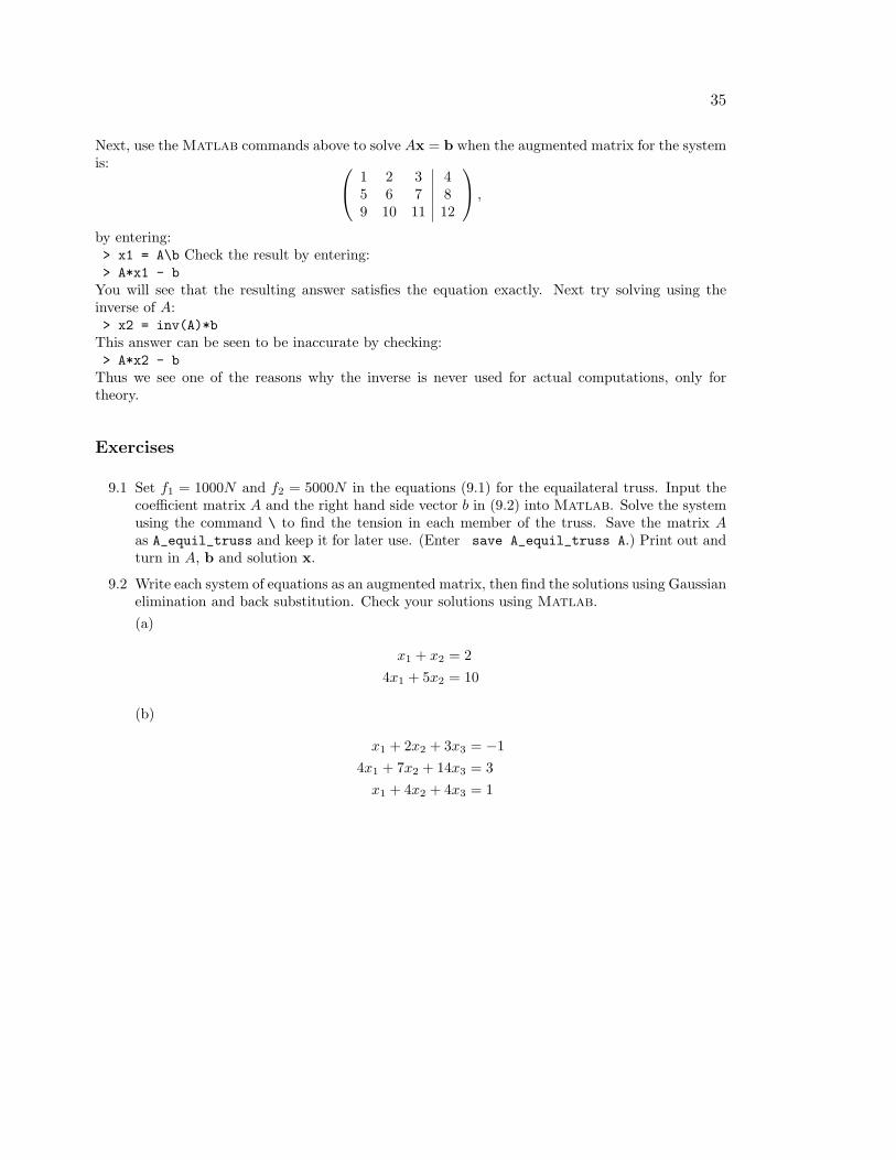
35

Next, use the Matlab commands above to solve Ax = b when the augmented matrix for the systemis:

1 2 3 45 6 7 89 10 11 12

,

by entering:> x1 = A\b Check the result by entering:> A*x1 - b

You will see that the resulting answer satisfies the equation exactly. Next try solving using theinverse of A:> x2 = inv(A)*b

This answer can be seen to be inaccurate by checking:> A*x2 - b

Thus we see one of the reasons why the inverse is never used for actual computations, only fortheory.

Exercises

9.1 Set f1 = 1000N and f2 = 5000N in the equations (9.1) for the equailateral truss. Input thecoefficient matrix A and the right hand side vector b in (9.2) into Matlab. Solve the systemusing the command \ to find the tension in each member of the truss. Save the matrix Aas A_equil_truss and keep it for later use. (Enter save A_equil_truss A.) Print out andturn in A, b and solution x.

9.2 Write each system of equations as an augmented matrix, then find the solutions using Gaussianelimination and back substitution. Check your solutions using Matlab.

(a)

x1 + x2 = 2

4x1 + 5x2 = 10

(b)

x1 + 2x2 + 3x3 = −1

4x1 + 7x2 + 14x3 = 3

x1 + 4x2 + 4x3 = 1

Lecture 10

Some Facts About Linear Systems

Some inconvenient truths

In the last lecture we learned how to solve a linear system using Matlab. Input the following:> A = ones(4,4)

> b = randn(4,1)

> x = A\b

As you will find, there is no solution to the equation Ax = b. This unfortunate circumstance ismostly the fault of the matrix, A, which is too simple, its columns (and rows) are all the same. Nowtry:> b = ones(4,1)

> x = [ 1 0 0 0]’

> A*x

So the system Ax = b does have a solution. Still unfortunately, that is not the only solution. Try:> x = [ 0 1 0 0]’

> A*x

We see that this x is also a solution. Next try: > x = [ -4 5 2.27 -2.27]’

> A*x

This x is a solution! It is not hard to see that there are endless possibilities for solutions of thisequation.

Basic theory

The most basic theoretical fact about linear systems is:

Theorem 1 A linear system Ax = b may have 0, 1, or infinitely many solutions.

Obviously, in most engineering applications we would want to have exactly one solution. Thefollowing two theorems show that having one and only one solution is a property of A.

Theorem 2 Suppose A is a square (n× n) matrix. The following are all equivalent:1. The equation Ax = b has exactly one solution for any b.2. det(A) 6= 0.3. A has an inverse.4. The only solution of Ax = 0 is x = 0.5. The columns of A are linearly independent (as vectors).6. The rows of A are linearly independent.

If A has these properties then it is called non-singular.

36

37

On the other hand, a matrix that does not have these properties is called singular.

Theorem 3 Suppose A is a square matrix. The following are all equivalent:1. The equation Ax = b has 0 or ∞ many solutions depending on b.2. det(A) = 0.3. A does not have an inverse.4. The equation Ax = 0 has solutions other than x = 0.5. The columns of A are linearly dependent as vectors.6. The rows of A are linearly dependent.

To see how the two theorems work, define two matrices (type in A1 then scroll up and modify tomake A2) :

A1 =

1 2 34 5 67 8 9

, A2 =

1 2 34 5 67 8 8

,

and two vectors:

b1 =

036

, b2 =

136

.

First calculate the determinants of the matrices:> det(A1)

> det(A2)

Then attempt to find the inverses:> inv(A1)

> inv(A2)

Which matrix is singular and which is non-singular? Finally, attempt to solve all the possibleequations Ax = b:> x = A1\b1

> x = A1\b2

> x = A2\b1

> x = A2\b2

As you can see, equations involving the non-singular matrix have one and only one solution, butequation involving a singular matrix are more complicated.

The residual vector

Recall that the residual for an approximate solution x of an equation f(x) = 0 is defined as r = f(x).It is a measure of how close the equation is to being satisfied. For a linear system of equations wedefine the residual of an approximate solution, x by

r = Ax− b. (10.1)

Notice that r is a vector. Its size (norm) is an indication of how close we have come to solvingAx = b.

38 LECTURE 10. SOME FACTS ABOUT LINEAR SYSTEMS

Exercises

10.1 By hand, find all the solutions (if any) of the following linear system using the augmentedmatrix and Gaussian elimination:

x1 + 2x2 + 3x3 = 4,

4x1 + 5x2 + 6x3 = 10, and

7x1 + 8x2 + 9x3 = 14 .

10.2 (a) Write a Matlab function program mysolvecheck with input a number n that makesa random n × n matrix A and a random vector b, solves the linear system Ax = b,calculates the norm of the residual r = Ax−b, and outputs that number as the error e.

(b) Write a Matlab script program that calls mysolvecheck 5 times each for n = 5, 10,50, 100, 500, 1000, . . ., records and averages the results, and makes a log-log plot of theaverage e vs. n.

Turn in the plot and the two programs.

Lecture 11

Accuracy, Condition Numbers andPivoting

In this lecture we will discuss two separate issues of accuracy in solving linear systems. The first,pivoting, is a method that ensures that Gaussian elimination proceeds as accurately as possible.The second, condition number, is a measure of how bad a matrix is. We will see that if a matrixhas a bad condition number, the solutions are unstable with respect to small changes in data.

The effect of rounding

All computers store numbers as finite strings of binary floating point digits. This limits numbers toa fixed number of significant digits and implies that after even the most basic calculations, roundingmust happen.

Consider the following exaggerated example. Suppose that our computer can only store 2 significantdigits and it is asked to do Gaussian elimination on:

(

.001 1 31 2 5

)

.

Doing the elimination exactly would produce:(

.001 1 30 −998 −2995

)

,

but rounding to 2 digits, our computer would store this as:(

.001 1 30 −1000 −3000

)

.

Backsolving this reduced system gives:

x1 = 0, x2 = 3.

This seems fine until you realize that backsolving the unrounded system gives:

x1 = −1, x2 = 3.001.

Row Pivoting

A way to fix the problem is to use pivoting, which means to switch rows of the matrix. Sinceswitching rows of the augmented matrix just corresponds to switching the order of the equations,

39

40 LECTURE 11. ACCURACY, CONDITION NUMBERS AND PIVOTING

no harm is done:(

1 2 5.001 1 3

)

.

Exact elimination would produce:(

1 2 50 .998 2.995

)

.

Storing this result with only 2 significant digits gives:

(

1 2 50 1 3

)

.

Now backsolving produces:x1 = −1, x2 = 3,

which is exactly right.

The reason this worked is because 1 is bigger than 0.001. To pivot we switch rows so that the largestentry in a column is the one used to eliminate the others. In bigger matrices, after each column iscompleted, compare the diagonal element of the next column with all the entries below it. Switchit (and the entire row) with the one with greatest absolute value. For example in the followingmatrix, the first column is finished and before doing the second column, pivoting should occur since| − 2| > |1|:

1 −2 3 40 1 6 70 −2 −10 −10

.

Pivoting the 2nd and 3rd rows would produce:

1 −2 3 40 −2 −10 −100 1 6 7

.

Condition number

In some systems, problems occur even without rounding. Consider the following augmented matri-ces:

(

1 1/2 3/21/2 1/3 1

)

and

(

1 1/2 3/21/2 1/3 5/6

)

.

Here we have the same A, but two different input vectors:

b1 = (3/2, 1)′ and b2 = (3/2, 5/6)′

which are pretty close to one another. You would expect then that the solutions x1 and x2 wouldalso be close. Notice that this matrix does not need pivoting. Eliminating exactly we get:

(

1 1/2 3/20 1/12 1/4

)

and

(

1 1/2 3/20 1/12 1/12

)

.

Now solving we find:x1 = (0, 3)′ and x2 = (1, 1)′

which are not close at all despite the fact that we did the calculations exactly. This poses a newproblem: some matrices are very sensitive to small changes in input data. The extent of this

41

sensitivity is measured by the condition number. The definition of condition number is: considerall small changes δA and δb in A and b and the resulting change, δx, in the solution x. Then:

cond(A) ≡ max

|δx|/|x||δA||A| + |δb|

|b|

= max

(

Relative error of output

Relative error of inputs

)

.

Put another way, changes in the input data get multiplied by the condition number to producechanges in the outputs. Thus a high condition number is bad. It implies that small errors in theinput can cause large errors in the output.

In Matlab enter:> H = hilb(2)

which should result in the matrix above. Matlab produces the condition number of a matrix withthe command:> cond(H)

Thus for this matrix small errors in the input can get magnified by 19 in the output. Next try thematrix:> A = [ 1.2969 0.8648 ; .2161 .1441]

> cond(A)

For this matrix small errors in the input can get magnified by 2.5× 108 in the output! (We will seethis happen in the exercise.) This is obviously not very good for engineering where all measurements,constants and inputs are approximate.

Is there a solution to the problem of bad condition numbers? Usually, bad condition numbers inengineering contexts result from poor design. So, the engineering solution to bad conditioning isredesign.

Finally, find the determinant of the matrix A above:> det(A)

which will be small. If det(A) = 0 then the matrix is singular, which is bad because it implies therewill not be a unique solution. The case here, det(A) ≈ 0, is also bad, because it means the matrix isalmost singular. Although det(A) ≈ 0 generally indicates that the condition number will be large,they are actually independent things. To see this, find the determinant and condition number ofthe matrix [1e-10,0;0,1e-10] and the matrix [1e+10,0;0,1e-10].

Exercises

11.1 Find the determinant and inverse of:

A =

[

1.2969 .8648.2161 .1441

]

.

Let B be the matrix obtained from A by rounding off to three decimal places (1.2969 7→ 1.297).Find the determinant and inverse of B. How do A−1 and B−1 differ? Explain how thishappened.

Set b1 = [1.2969; 0.2161] and do x = A\b1 . Repeat the process but with a vector b2obtained from b1 by rounding off to three decimal places. Explain exactly what happened.Why was the first answer so simple? Why do the two answers differ by so much?

42 LECTURE 11. ACCURACY, CONDITION NUMBERS AND PIVOTING

11.2 Try> B = [sin(sym(1)) sin(sym(2)); sin(sym(3)) sin(sym(4))]

> c = [1; 2]

> x = B\c

> pretty(x)

Next input the matrix:

Cs =

[

1 22 4

]

symbolically as above. Create a numerical version via Cn = double(Cs) and define thetwo vectors d1 = [4; 8] and d2 = [1; 1]. Solve the systems Cs*x = d1, Cn*x = d1,Cs*x = d2, and Cn*x = d2. Explain the results. Does the symbolic or non-symbolic way givemore information?

11.3 Recall the matrix A that you saved using A_equil_truss. (Enter > load A_equil_truss orclick on the file A_equil_truss.mat in the folder where you saved it. This should reproducethe matrix A.

Find the condition number for this matrix. Is it good or bad? Now change any of the entriesin A and recalculate the condition number and compare. What does this say about theequilateral truss?

Lecture 12

LU Decomposition

In many applications where linear systems appear, one needs to solve Ax = b for many differentvectors b. For instance, a structure must be tested under several different loads, not just one. As inthe example of a truss (9.2), the loading in such a problem is usually represented by the vector b.Gaussian elimination with pivoting is the most efficient and accurate way to solve a linear system.Most of the work in this method is spent on the matrix A itself. If we need to solve several differentsystems with the same A, and A is big, then we would like to avoid repeating the steps of Gaussianelimination on A for every different b. This can be accomplished by the LU decomposition, whichin effect records the steps of Gaussian elimination.

LU decomposition

The main idea of the LU decomposition is to record the steps used in Gaussian elimination on A inthe places where the zero is produced. Consider the matrix:

A =

1 −2 32 −5 120 2 −10

.

The first step of Gaussian elimination is to subtract 2 times the first row from the second row. Inorder to record what we have done, we will put the multiplier, 2, into the place it was used to makea zero, i.e. the second row, first column. In order to make it clear that it is a record of the step andnot an element of A, we will put it in parentheses. This leads to:

1 −2 3(2) −1 60 2 −10

.

There is already a zero in the lower left corner, so we don’t need to eliminate anything there. Werecord this fact with a (0). To eliminate the third row, second column, we need to subtract −2times the second row from the third row. Recording the −2 in the spot it was used we have:

1 −2 3(2) −1 6(0) (−2) 2

.

Let U be the upper triangular matrix produced, and let L be the lower triangular matrix with therecords and ones on the diagonal, i.e.:

L =

1 0 02 1 00 −2 1

, U =

1 −2 30 −1 60 0 2

,

43

44 LECTURE 12. LU DECOMPOSITION

then we have the following mysterious coincidence:

LU =

1 0 02 1 00 −2 1

1 −2 30 −1 60 0 2

=

1 −2 32 −5 120 2 −10

= A.

Thus we see that A is actually the product of L and U . Here L is lower triangular and U isupper triangular. When a matrix can be written as a product of simpler matrices, we call that adecomposition of A and this one we call the LU decomposition.

Using LU to solve equations

If we also include pivoting, then an LU decomposition for A consists of three matrices P , L and Usuch that:

PA = LU. (12.1)

The pivot matrix P is the identity matrix, with the same rows switched as the rows of A are switchedin the pivoting. For instance:

P =

1 0 00 0 10 1 0

,

would be the pivot matrix if the second and third rows of A are switched by pivoting. Matlab willproduce an LU decomposition with pivoting for a matrix A with the following command:> [L U P] = lu(A)

where P is the pivot matrix. To use this information to solve Ax = b we first pivot both sides bymultiplying by the pivot matrix:

PAx = Pb ≡ d.

Substituting LU for PA we get:LUx = d.

Then we need only to solve two back substitution problems:

Ly = d

andUx = y.

In Matlab this would work as follows:> A = rand(5,5)

> [L U P] = lu(A)

> b = rand(5,1)

> d = P*b

> y = L\d

> x = U\y

> rnorm = norm(A*x - b) . . . . . . . . . . . . . . . . . . . . . . . . . . . . . . . . . . . . . . . . . . . . . . . . . Check the result.We can then solve for any other b without redoing the LU step. Repeat the sequence for a newright hand side: c = randn(5,1); you can start at the third line. While this may not seem like abig savings, it would be if A were a large matrix from an actual application.

45

Exercises

12.1 Solve the systems below by hand using the LU decomposition. Pivot if appropriate. In eachof the two problems, check by hand that LU = PA and Ax = b.

(a) A =

(

2 4.5 4

)

, b =

(

0−3

)

(b) A =

(

1 43 5

)

, b =

(

32

)

12.2 Finish the following Matlab function program:

function [x1, e1, x2, e2] = mysolve(A,b)

% Solves linear systems using the LU decomposition with pivoting

% and also with the built-in solve function A\b.

% Inputs: A -- the matrix

% b -- the right-hand vector

% Outputs: x1 -- the solution using the LU method

% e1 -- the norm of the residual using the LU method

% x2 -- the solution using the built-in method

% e2 -- the norm of the residual using the built-in method

format long

Test the program on both random matrices (randn(n,n)) and Hilbert matrices (hilb(n))with n large (as big as you can make it and the program still run) and document the results.

Lecture 13

Nonlinear Systems - Newton’s Method

An Example

The LORAN (LOng RAnge Navigation) system calculates the position of a boat at sea using signalsfrom fixed transmitters. From the time differences of the incoming signals, the boat obtains dif-ferences of distances to the transmitters. This leads to two equations each representing hyperbolasdefined by the differences of distance of two points (foci). An example of such equations from [2]are:

x2

1862− y2

3002 − 1862= 1 and

(y − 500)2

2792− (x− 300)2

5002 − 2792= 1 .

(13.1)

Solving two quadratic equations with two unknowns, would require solving a 4 degree polynomialequation. We could do this by hand, but for a navigational system to work well, it must do thecalculations automatically and numerically. We note that the Global Positioning System (GPS)works on similar principles and must do similar computations.

Vector Notation

In general, we can usually find solutions to a system of equations when the number of unknownsmatches the number of equations. Thus, we wish to find solutions to systems that have the form:

f1(x1, x2, x3, . . . , xn) = 0

f2(x1, x2, x3, . . . , xn) = 0

f3(x1, x2, x3, . . . , xn) = 0

...

fn(x1, x2, x3, . . . , xn) = 0.

(13.2)

For convenience we can think of (x1, x2, x3, . . . , xn) as a vector x and (f1, f2, . . . , fn) as a vector-valued function f . With this notation, we can write the system of equations (13.2) simply as:

f(x) = 0,

i.e. we wish to find a vector that makes the vector function equal to the zero vector.

As in Newton’s method for one variable, we need to start with an initial guess x0. In theory, the morevariables one has, the harder it is to find a good initial guess. In practice, this must be overcome by

46

47

using physically reasonable assumptions about the possible values of a solution, i.e. take advantageof engineering knowledge of the problem. Once x0 is chosen, let

∆x = x1 − x0.

Linear Approximation for Vector Functions

In the single variable case, Newton’s method was derived by considering the linear approximationof the function f at the initial guess x0. From Calculus, the following is the linear approximationof f at x0, for vectors and vector-valued functions:

f(x) ≈ f(x0) +Df(x0)(x− x0).

Here Df(x0) is an n× n matrix whose entries are the various partial derivative of the componentsof f . Specifically:

Df(x0) =

∂f1∂x1

(x0)∂f1∂x2

(x0)∂f1∂x3

(x0) . . . ∂f1∂xn

(x0)

∂f2∂x1

(x0)∂f2∂x2

(x0)∂f2∂x3

(x0) . . . ∂f2∂xn

(x0)

......

.... . .

...

∂fn∂x1

(x0)∂fn∂x2

(x0)∂fn∂x3

(x0) . . . ∂fn∂xn

(x0)

. (13.3)

Newton’s Method

We wish to find x that makes f equal to the zero vectors, so let’s choose x1 so that

f(x0) +Df(x0)(x1 − x0) = 0.

Since Df(x0) is a square matrix, we can solve this equation by

x1 = x0 − (Df(x0))−1f(x0),

provided that the inverse exists. The formula is the vector equivalent of the Newton’s method for-mula we learned before. However, in practice we never use the inverse of a matrix for computations,so we cannot use this formula directly. Rather, we can do the following. First solve the equation

Df(x0)∆x = −f(x0). (13.4)

Since Df(x0) is a known matrix and −f(x0) is a known vector, this equation is just a system oflinear equations, which can be solved efficiently and accurately. Once we have the solution vector∆x, we can obtain our improved estimate x1 by:

x1 = x0 +∆x.

For subsequent steps, we have the following process:

• Solve Df(xi)∆x = −f(xi) for ∆x.

• Let xi+1 = xi +∆x

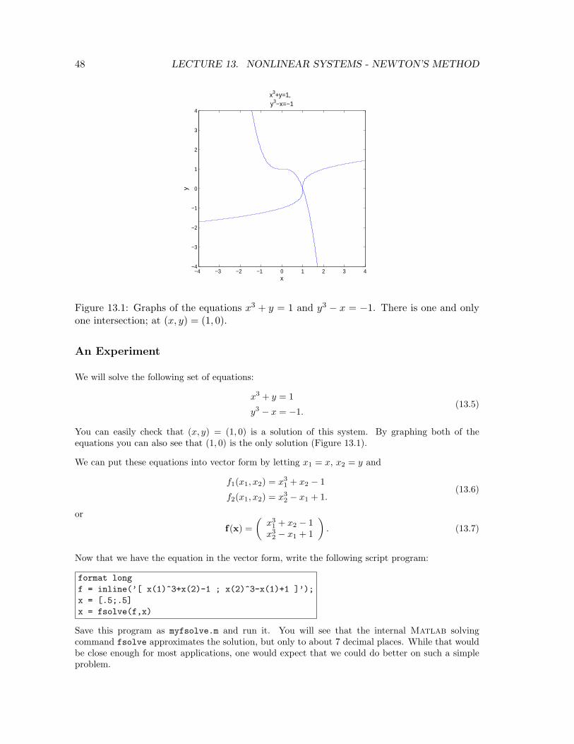
48 LECTURE 13. NONLINEAR SYSTEMS - NEWTON’S METHOD

−4 −3 −2 −1 0 1 2 3 4−4

−3

−2

−1

0

1

2

3

4

x

y

x3+y=1, y3−x=−1

Figure 13.1: Graphs of the equations x3 + y = 1 and y3 − x = −1. There is one and onlyone intersection; at (x, y) = (1, 0).

An Experiment

We will solve the following set of equations:

x3 + y = 1

y3 − x = −1.(13.5)

You can easily check that (x, y) = (1, 0) is a solution of this system. By graphing both of theequations you can also see that (1, 0) is the only solution (Figure 13.1).

We can put these equations into vector form by letting x1 = x, x2 = y and

f1(x1, x2) = x31 + x2 − 1

f2(x1, x2) = x32 − x1 + 1.

(13.6)

or

f(x) =

(

x31 + x2 − 1

x32 − x1 + 1

)

. (13.7)

Now that we have the equation in the vector form, write the following script program:

format long

f = inline(’[ x(1)^3+x(2)-1 ; x(2)^3-x(1)+1 ]’);

x = [.5;.5]

x = fsolve(f,x)

Save this program as myfsolve.m and run it. You will see that the internal Matlab solvingcommand fsolve approximates the solution, but only to about 7 decimal places. While that wouldbe close enough for most applications, one would expect that we could do better on such a simpleproblem.

49

Next we will implement Newton’s method for this problem. Modify your myfsolve program to:

% mymultnewton

format long

n=8 % set some number of iterations, may need adjusting

f = inline(’[x(1)^3+x(2)-1 ; x(2)^3-x(1)+1]’); % the vector function

Df = inline(’[3*x(1)^2, 1 ; -1, 3*x(2)^2]’); % the matrix of partial derivatives

x = [.5;.5] % starting guess

for i = 1:n

Dx = -Df(x)\f(x); % solve for increment

x = x + Dx % add on to get new guess

f(x) % see if f(x) is really zero

end

Save and run this program (as mymultnewton) and you will see that it finds the root exactly (tomachine precision) in only 6 iterations. Why is this simple program able to do better thanMatlab’sbuilt-in program?

Exercises

13.1 (a) Put the LORAN equations (13.1) into the function form (13.2).

(b) Construct the matrix of partial derivatives Df in (13.3).

(c) Adapt the mymultnewton program to find a solution for these equations. By tryingdifferent starting vectors, find at least three different solutions. (There are actually foursolutions.) Think of at least one way that the navigational system could determinewhich solution is correct.

Lecture 14

Eigenvalues and Eigenvectors

Suppose that A is a square (n× n) matrix. We say that a nonzero vector v is an eigenvector (ev)and a number λ is its eigenvalue (ew) if

Av = λv. (14.1)

Geometrically this means that Av is in the same direction as v, since multiplying a vector by anumber changes its length, but not its direction.

Matlab has a built-in routine for finding eigenvalues and eigenvectors:> A = pascal(4)

> [v e] = eig(A)

The results are a matrix v that contains eigenvectors as columns and a diagonal matrix e thatcontains eigenvalues on the diagonal. We can check this by:> v1 = v(:,1)

> A*v1

> e(1,1)*v1

Finding Eigenvalues for 2× 2 and 3× 3

If A is 2×2 or 3×3 then we can find its eigenvalues and eigenvectors by hand. Notice that Equation(14.1) can be rewritten as:

Av − λv = 0. (14.2)

It would be nice to factor out the v from the right-hand side of this equation, but we can’t becauseA is a matrix and λ is a number. However, since Iv = v, we can do the following:

Av − λv = Av − λIv

= (A− λI)v

= 0

(14.3)

If v is nonzero, then by Theorem 3 in Lecture 10 the matrix (A − λI) must be singular. By thesame theorem, we must have:

det(A− λI) = 0. (14.4)

This is called the characteristic equation.

50

51

For a 2× 2 matrix, A− λI is calculated as in the following example:

A− λI =

(

1 43 5

)

− λ

(

1 00 1

)

=

(

1 43 5

)

−(

λ 00 λ

)

=

(

1− λ 43 5− λ

)

.

(14.5)

The determinant of A− λI is then

det(A− λI) = (1− λ)(5− λ)− 4 · 3= −7− 6λ+ λ2.

(14.6)

The characteristic equation det(A− λI) = 0 is simply a quadratic equation:

λ2 − 6λ− 7 = 0. (14.7)

The roots of this equation are λ1 = 7 and λ2 = −1. These are the ew’s of the matrix A. Now tofind the corresponding ev’s we return to the equation (A− λI)v = 0. For λ1 = 7, the equation forthe ev (A− λI)v = 0 is equivalent to the augmented matrix

(

−6 4 03 −2 0

)

. (14.8)

Notice that the first and second rows of this matrix are multiples of one another. Thus Gaussianelimination would produce all zeros on the bottom row. Thus this equation has infinitely manysolutions, i.e. infinitely many ev’s. Since only the direction of the ev matters, this is okay, we onlyneed to find one of the ev’s. Since the second row of the augmented matrix represents the equation

3x− 2y = 0,

we can let

v1 =

(

23

)

.

This comes from noticing that (x, y) = (2, 3) is a solution of 3x− 2y = 0.

For λ2 = −1, (A− λI)v = 0 is equivalent to the augmented matrix:(

2 4 03 6 0

)

.

Once again the first and second rows of this matrix are multiples of one another. For simplicity wecan let

v2 =

(

−21

)

.

One can always check an ev and ew by multiplying:

Av1 =

(

1 43 5

)(

23

)

=

(

1421

)

= 7

(

23

)

= 7v1 and

Av2 =

(

1 43 5

)(

−21

)

=

(

2−1

)

= −1

(

−21

)

= −1v2 .

For a 3 × 3 matrix we could complete the same process. The det(A − λI) = 0 would be a cubicpolynomial and we would expect to usually get 3 roots, which are the ew’s.

52 LECTURE 14. EIGENVALUES AND EIGENVECTORS

Larger Matrices

For a n × n matrix with n ≥ 4 this process is too long and cumbersome to complete by hand.Further, this process is not well suited even to implementation on a computer program since itinvolves determinants and solving a n-degree polynomial. For n ≥ 4 we need more ingeniousmethods. These methods rely on the geometric meaning of ev’s and ew’s rather than solvingalgebraic equations. We will overview these methods in Lecture 16.

Complex Eigenvalues

It turns out that the eigenvalues of some matrices are complex numbers, even when the matrix onlycontains real numbers. When this happens the complex ew’s must occur in conjugate pairs, i.e.:

λ1,2 = α± iβ.

The corresponding ev’s must also come in conjugate pairs:

w = u± iv.

In applications, the imaginary part of the ew, β, often is related to the frequency of an oscillation.This is because of Euler’s formula

eα+iβ = eα(cosβ + i sinβ).

Certain kinds of matrices that arise in applications can only have real ew’s and ev’s. The mostcommon such type of matrix is the symmetric matrix. A matrix is symmetric if it is equal to itsown transpose, i.e. it is symmetric across the diagonal. For example,

(

1 33 −5

)

is symmetric and so we know beforehand that its ew’s will be real, not complex.

Exercises

14.1 Find the eigenvalues and eigenvectors of the following matrix by hand:

A =

(

2 11 2

)

.

14.2 Find the eigenvalues and eigenvectors of the following matrix by hand:

B =

(

1 −22 1

)

.

Can you guess the ew’s of the matrix

C =

(

a −bb a

)

?

Lecture 15

An Application of Eigenvectors:Vibrational Modes

One application of ew’s and ev’s is in the analysis of vibration problems. A simple nontrivialvibration problem is the motion of two objects with equal masses m attached to each other andfixed outer walls by equal springs with spring constants k, as shown in Figure 15.1.

Let x1 denote the displacement of the first mass and x2 the displacement of the second, and notethe displacement of the walls is zero. Each mass experiences forces from the adjacent springsproportional to the stretch or compression of the spring. Ignoring any friction, Newton’s law ofmotion ma = F , leads to:

mx1 = −k(x1 − 0) +k(x2 − x1) = −2kx1 + kx2

mx2 = −k(x2 − x1) +k(0− x2) = kx1 − 2kx2. (15.1)

Dividing both sides by m we can write these equations in matrix form:

x = −Ax, (15.2)

where

A =k

mB =

k

m

(

2 −1−1 2

)

. (15.3)

For this type of equation, the general solution is:

x(t) = c1v1 sin

(√

kλ1

mt+ φ1

)

+ c2v2 sin

(√

kλ2

mt+ φ2

)

(15.4)

where λ1 and λ2 are ew’s of B with corresponding ev’s v1 and v2. One can check that this is asolution by substituting it into the equation (15.2).

We can interpret the ew’s as the squares of the frequencies of oscillation. We can find the ew’s andev’s of B using Matlab:> B = [2 -1 ; -1 2]

> [v e] = eig(B)

This should produce a matrix v whose columns are the ev’s of B and a diagonal matrix e whose

u u-x1

-x2

Figure 15.1: Two equal masses attached to each other and fixed walls by equal springs.

53

54LECTURE 15. AN APPLICATION OF EIGENVECTORS: VIBRATIONAL MODES

u u

u u

u u

u u

u u

u u

u u

u u

u u

u u

Figure 15.2: Two vibrational modes of a simple oscillating system. In the left mode theweights move together and in the right mode they move opposite. Note that the two modesactually move at different speeds.

entries are the ew’s of B. In the first eigenvector, v1, the two entries are equal. This represents themode of oscillation where the two masses move in sync with each other. The second ev, v2, has thesame entries but opposite signs. This represents the mode where the two masses oscillate in anti-synchronization. Notice that the frequency for anti-sync motion is

√3 times that of synchronous

motion.

Which of the two modes is the most dangerous for a structure or machine? It is the one with thelowest frequency because that mode can have the largest displacement. Sometimes this mode iscalled the fundamental mode.

To get the frequencies for the matrix A = k/mB, notice that if vi is one of the ev’s for B then:

Avi =k

mBvi =

k

mλivi.

Thus we can conclude that A has the same ev’s as B, but the ew’s are multiplied by the factork/m. Thus the two frequencies are:

√

k

mand

√

3k

m.

We can do the same for three equal masses. The corresponding matrix B would be:

B =

2 −1 0−1 2 −10 −1 2

.

Find the ev’s and ew’s as above. There are three different modes. Interpret them from the ev’s.

55

Exercises

15.1 Find the frequencies and modes for 4 equal masses with equal springs. Interpret the modes.

15.2 Find the frequencies and modes for non-identical masses with equal springs in the followingcases. How does this effect the modes?

(a) Two masses with m1 = 1 and m2 = 2.

(b) Three masses with m1 = 1, m2 = 2 and m3 = 3.

Lecture 16

Numerical Methods for Eigenvalues

As mentioned above, the ew’s and ev’s of an n× n matrix where n ≥ 4 must be found numericallyinstead of by hand. The numerical methods that are used in practice depend on the geometricmeaning of ew’s and ev’s which is equation (14.1). The essence of all these methods is captured inthe Power method, which we now introduce.

The Power Method

In the command window of Matlab enter the following:> A = hilb(5)

> x = ones(5,1)

> x = A*x

> el = max(x)

> x = x/el

Compare the new value of x with the original. Repeat the last three lines (you can use the scroll upbutton). Compare the newest value of x with the previous one and the original. Notice that there isless change between the second two. Repeat the last three commands over and over until the valuesstop changing. You have completed what is known as the Power Method. Now try the command:> [v e] = eig(A)

The last entry in e should be the final el we computed. The last column in v is x/norm(x). Belowwe explain why our commands gave this eigenvalue and eigenvector.

For illustration consider a 2× 2 matrix whose ew’s are 1/3 and 2 and whose corresponding ev’s arev1 and v2. Let x0 be any vector which is a combination of v1 and v2, e.g.,

x0 = v1 + v2.

Now let x1 be A times x0. It follows from (14.1) that

x1 = Av1 +Av2

=1

3v1 + 2v2.

(16.1)

Thus the v1 part is shrunk while the v2 is stretched. If we repeat this process k times then:

xk = Axk−1

= Akx0

=

(

1

3

)k

v1 + 2kv2.

(16.2)

56

57

Clearly, xk grows in the direction of v2 and shrinks in the direction of v1. This is the principle ofthe Power Method, vectors multiplied by A are stretched most in the direction of the ev whose ewhas the largest absolute value.

The ew with the largest absolute value is called the dominant ew. In many applications thisquantity will necessarily be positive for physical reasons. When this is the case, the Matlab codeabove will work since max(v) will be the element with the largest absolute value. In applicationswhere the dominant ew may be negative, the program must use flow control to determine the correctnumber.

Summarizing the Power Method:

• Repeatedly multiply x by A and divide by the element with the largest absolute value.

• The element of largest absolute value converges to largest absolute ew.

• The vector converges to the corresponding ev.

Note that this logic only works when the eigenvalue largest in magnitude is real. If the matrix andstarting vector are real then the power method can never give a result with an imaginary part.Eigenvalues with imaginary part mean the matrix has a rotational component, so the eigenvectorwould not settle down either.

Try:> A = rand(15,11) ;

> e = eig(A)

You can see that for a random square matrix, many of the ew’s are complex.

However, matrices in applications are not just random. They have structure, and this can lead toreal eigenvalues as seen in the next section.

Symmetric, Positive-Definite Matrices

As noted in the previous paragraph, the power method can fail if A has complex eigenvalues. Oneclass of matrices that appear often in applications and for which the eigenvalues are always real arecalled the symmetric matrices. A matrix is symmetric if:

A′ = A,

i.e. A is symmetric with respect to reflections about its diagonal.

Try:> A = rand(5,5)

> C = A’*A

> e = eig(C)

You can see that the eigenvalues of these symmetric matrices are real.

Next we consider an even more specialized class for which the eigenvalues are not only real, butpositive. A symmetric matrix is called positive definite if for all vectors v 6= 0 the following holds:

Av · v > 0.

Geometrically, A does not rotate any vector by more than 180 degrees. In summary:

58 LECTURE 16. NUMERICAL METHODS FOR EIGENVALUES

• If A is symmetric then its eigenvalues are real.

• If A is symmetric positive definite, then its eigenvalues are positive numbers.

Notice that the B matrices in the previous section were symmetric and the ew’s were all real. Noticethat the Hilbert and Pascal matrices are symmetric.

The Inverse Power Method

In the application of vibration analysis, the mode (ev) with the lowest frequency (ew) is the mostdangerous for the machine or structure. The Power Method gives us instead the largest ew, whichis the least important frequency. In this section we introduce a method, the Inverse Power Methodwhich produces exactly what is needed.

The following facts are at the heart of the Inverse Power Method:

• If λ is an ew of A then 1/λ is an ew for A−1.

• The ev’s for A and A−1 are the same.

Thus if we apply the Power Method to A−1 we will obtain the largest absolute ew of A−1, which isexactly the reciprocal of the smallest absolute ew of A. We will also obtain the corresponding ev,which is an ev for both A−1 and A. Recall that in the application of vibration mode analysis, thesmallest ew and its ev correspond exactly to the frequency and mode that we are most interestedin, i.e. the one that can do the most damage.

Here as always, we do not really want to calculate the inverse of A directly if we can help it.Fortunately, multiplying xi by A−1 to get xi+1 is equivalent to solving the system:

Axi+1 = xi ,

which can be done efficiently and accurately. Since iterating this process involves solving a linearsystem with the same A but many different right hand sides, it is a perfect time to use the LUdecomposition to save computations. The following function program does n steps of the InversePower Method.

function [v e] = myipm(A,n)

[L U P] = lu(A); % LU decomposition of A with pivoting

m = size(A,1);

v = ones(m,1); % make an initial vector with ones

for i = 1:n

pv = P*v;

y = L\pv;

v = U\y;

M = max(v);

m = min(v);

if abs(M) >= abs(m)

el = M;

else

el = m;

end

v = v/el;

end

e = 1/el;

59

Exercises

16.1 For each of the following matrices, perform one interation of the power method by handstarting with a vector of all ones. State the resulting approximations of the eigenvalue andeigenvector.

A =

[

1 23 4

]

(16.3)

B =

−2 1 01 −2 10 1 −2

(16.4)

16.2 (a) Write a Matlab function program mypm that inputs a matrix and a tolerance, appliesthe power method until the change in the vector is less than the tolerance, and outputsthe number of steps used and the estimated eigenvalue and eigenvector.

(b) Test your program on the matrices A and B in the previous exercise.

Lecture 17

The QR Method*

The Power Method and Inverse Power Method each give us only one ew–ev pair. While both ofthese methods can be modified to give more ew’s and ev’s, there is a better method for obtainingall the ew’s called the QR method. This is the basis of all modern ew software, including Matlab,so we summarize it briefly here.

The QR method uses the fact that any square matrix has a QR decomposition. That is, for any Athere are matrices Q and R such the A = QR where Q has the property

Q−1 = Q′

and R is upper triangular. A matrix Q with the property that its transpose equals its inverse iscalled an orthogonal matrix, because its column vectors are mutually orthogonal.

The QR method consists of iterating following steps:- Transform A into a tridiagonal matrix H.- decompose H in QR.- multiply Q and R together in reverse order to form a new H.The diagonal of H will converge to the eigenvalues.

We details of what makes this method converge are beyond the scope of the this book. However,we note the following theory behind it for those with more familiarity with linear algrebra. Firstthe Hessian matrix H is obtained from A by a series of similarity transformation, thus it has thesame ew’s as A. Secondly, if we denote by H0, H1, H2, . . ., the sequence of matrices produced bythe iteration, then

Hi+1 = RiQi = Q−1i QiRiQi = Q′

iHiQi.

Thus each Hi+1 is a related to Hi by an (orthogonal) simularity transformation and so they havethe same ew’s as A.

There is a built-in QR decomposition inMatlab which is called with the command: [Q R] = qr(A).Thus the following program implements QR method until it converges:

60

61

function E = myqrmethod(A)

[m n] = size(A);

if m ~= n

warning(’The input matrix is not square.’)

return

end

H = hess(A);

E = diag(H);

change = 1;

steps = 0;

while change > 0

Eold = E;

[Q R] = qr(H);

H = R*Q;

E = diag(H);

change = norm(E - Eold);

steps = steps +1;

end

steps

As you can see the main steps of the program are very simple. The really hard calculations arecontained in the built-in command qr(A).

Run this program and compare the results with Matlab’s built in command:> format long

> format compact

> A = hilb(5)

> Eqr = myqrmtheod(A)

> Eml =eig(A)

Exercises

17.1 Modify myqrmethod to stop after a maximum number of iterations. Use the modified program,with the maximum iterations set to 1000, on the matrix A = hilb(n) with n equal to 10, 50,and 200. Use the norm to compare the results to the ew’s obtained from Matlab’s built-inprogram eig. Turn in a printout of your program and a brief report on the experiment.

Lecture 18

Iterative solution of linear systems*

Newton refinement

Conjugate gradient method

62

Review of Part II

Methods and Formulas

Basic Matrix Theory:Identity matrix: AI = A, IA = A, and Iv = vInverse matrix: AA−1 = I and A−1A = INorm of a matrix: |A| ≡ max|v|=1 |Av|A matrix may be singular or nonsingular. See Lecture 10.

Solving Process:Gaussian Elimination produces LU decompositionRow PivotingBack Substitution

Condition number:

cond(A) ≡ max

|δx|/|x||δA||A| + |δb|

|b|

= max

(

Relative error of output

Relative error of inputs

)

.

A big condition number is bad; in engineering it usually results from poor design.

LU factorization:PA = LU.

Solving steps:Multiply by P: d = PbForwardsolve: Ly = dBacksolve: Ux = y

Eigenvalues and eigenvectors:A nonzero vector v is an eigenvector (ev) and a number λ is its eigenvalue (ew) if

Av = λv.

Characteristic equation: det(A− λI) = 0Equation of the eigenvector: (A− λI)v = 0

Complex ew’s:Occur in conjugate pairs: λ1,2 = α± iβand ev’s must also come in conjugate pairs: w = u± iv.

Vibrational modes:Eigenvalues are frequencies squared. Eigenvectors are modes.

63

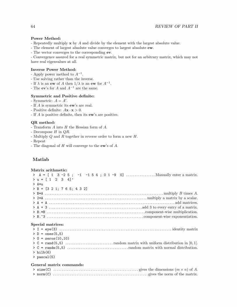
64 REVIEW OF PART II

Power Method:- Repeatedly multiply x by A and divide by the element with the largest absolute value.- The element of largest absolute value converges to largest absolute ew.- The vector converges to the corresponding ev.- Convergence assured for a real symmetric matrix, but not for an arbitrary matrix, which may nothave real eigenvalues at all.

Inverse Power Method:- Apply power method to A−1.- Use solving rather than the inverse.- If λ is an ew of A then 1/λ is an ew for A−1.- The ev’s for A and A−1 are the same.

Symmetric and Positive definite:- Symmetric: A = A′.- If A is symmetric its ew’s are real.- Positive definite: Ax · x > 0.- If A is positive definite, then its ew’s are positive.

QR method:- Transform A into H the Hessian form of A.- Decompose H in QR.- Multiply Q and R together in reverse order to form a new H.- Repeat- The diagonal of H will converge to the ew’s of A.

Matlab

Matrix arithmetic:> A = [ 1 3 -2 5 ; -1 -1 5 4 ; 0 1 -9 0] . . . . . . . . . . . . . . . . . Manually enter a matrix.> u = [ 1 2 3 4]’

> A*u

> B = [3 2 1; 7 6 5; 4 3 2]

> B*A . . . . . . . . . . . . . . . . . . . . . . . . . . . . . . . . . . . . . . . . . . . . . . . . . . . . . . . . . . . . . . . . . . . . . .multiply B times A.> 2*A . . . . . . . . . . . . . . . . . . . . . . . . . . . . . . . . . . . . . . . . . . . . . . . . . . . . . . . . . . . . multiply a matrix by a scalar.> A + A . . . . . . . . . . . . . . . . . . . . . . . . . . . . . . . . . . . . . . . . . . . . . . . . . . . . . . . . . . . . . . . . . . . . . . . . . . add matrices.> A + 3 . . . . . . . . . . . . . . . . . . . . . . . . . . . . . . . . . . . . . . . . . . . . . . . . . . . . . . .add 3 to every entry of a matrix.> B.*B . . . . . . . . . . . . . . . . . . . . . . . . . . . . . . . . . . . . . . . . . . . . . . . . . . . . . . . . . . component-wise multiplication.> B.^3 . . . . . . . . . . . . . . . . . . . . . . . . . . . . . . . . . . . . . . . . . . . . . . . . . . . . . . . . . component-wise exponentiation.

Special matrices:> I = eye(3) . . . . . . . . . . . . . . . . . . . . . . . . . . . . . . . . . . . . . . . . . . . . . . . . . . . . . . . . . . . . . . . . . . identity matrix> D = ones(5,5)

> O = zeros(10,10)

> C = rand(5,5) . . . . . . . . . . . . . . . . . . . . . . . . . . . . random matrix with uniform distribution in [0, 1].> C = randn(5,5) . . . . . . . . . . . . . . . . . . . . . . . . . . . . . . . . . . . . random matrix with normal distribution.> hilb(6)

> pascal(5)

General matrix commands:> size(C) . . . . . . . . . . . . . . . . . . . . . . . . . . . . . . . . . . . . . . . . . . . . . . . . . . gives the dimensions (m× n) of A.> norm(C) . . . . . . . . . . . . . . . . . . . . . . . . . . . . . . . . . . . . . . . . . . . . . . . . . . . . . . . . gives the norm of the matrix.

65

> det(C) . . . . . . . . . . . . . . . . . . . . . . . . . . . . . . . . . . . . . . . . . . . . . . . . . . . . . . . . the determinant of the matrix.> max(C) . . . . . . . . . . . . . . . . . . . . . . . . . . . . . . . . . . . . . . . . . . . . . . . . . . . . . . . . . . . . the maximum of each row.> min(C) . . . . . . . . . . . . . . . . . . . . . . . . . . . . . . . . . . . . . . . . . . . . . . . . . . . . . . . . . . . . the minimum in each row.> sum(C) . . . . . . . . . . . . . . . . . . . . . . . . . . . . . . . . . . . . . . . . . . . . . . . . . . . . . . . . . . . . . . . . . . . . . . . sums each row.> mean(C) . . . . . . . . . . . . . . . . . . . . . . . . . . . . . . . . . . . . . . . . . . . . . . . . . . . . . . . . . . . . . the average of each row.> diag(C) . . . . . . . . . . . . . . . . . . . . . . . . . . . . . . . . . . . . . . . . . . . . . . . . . . . . . . . . . . just the diagonal elements.> inv(C) . . . . . . . . . . . . . . . . . . . . . . . . . . . . . . . . . . . . . . . . . . . . . . . . . . . . . . . . . . . . . . . . . inverse of the matrix.> C’ . . . . . . . . . . . . . . . . . . . . . . . . . . . . . . . . . . . . . . . . . . . . . . . . . . . . . . . . . . . . . . . . . . . transpose of the matrix.

Matrix decompositions:> [L U P] = lu(C)

> [Q R] = qr(C)

> [U S V] = svd(C) . . . . . . . . . . singular value decomposition (important, but we did not use it).> H = hess(C) transform into a Hessian tri-diagonal matrix. A matrix that has the same eigen-

values as A. > [U T] = schur(C) . . . . . . . . . . . . . . . . . . . . . . . . . . Schur Decomposition A = U ′TU .> R = chol(C*C’) Cholesky decomposition of a symmetric, positive definite matrix, A = R′R.

66 REVIEW OF PART II

Part III

Functions and Data

c©Copyright, Todd Young and Martin Mohlenkamp, Mathematics Department, Ohio University, 2007

Lecture 19

Polynomial and Spline Interpolation

A Chemical Reaction

In a chemical reaction the concentration level y of the product at time t was measured every halfhour. The following results were found:t 0 .5 1.0 1.5 2.0y 0 .19 .26 .29 .31

We can input this data into Matlab as:> t1 = 0:.5:2

> y1 = [ 0 .19 .26 .29 .31 ]

and plot the data with:> plot(t1,y1)

Matlab automatically connects the data with line segments. This is the simplest form of interpo-lation, meaning fitting a graph (of a function) between data points. What if we want a smoothergraph? Try:> plot(t1,y1,’*’)

which will produce just asterisks at the data points. Next click on Tools, then click on theBasic Fitting option. This should produce a small window with several fitting options. Beginclicking them one at a time, clicking them off before clicking the next. Which ones produce a good-looking fit? You should note that the spline, the shape-preserving interpolant and the 4th degreepolynomial produce very good curves. The others do not. We will discuss polynomial interpolationand spline interpolation in this lecture.

Polynomial Fitting

The most general degree n polynomial is:

pn(x) = anxn + an−1x

n−1 + . . .+ a1x+ a0.

If we have exactly n + 1 data points, that is enough to exactly determine the n + 1 coefficients ofpn(x) (as long as the data does not have repeated x values). If there are more data points, thatwould give us an overdetermined system (more equations than unknowns) and if there is less datathe system would be undetermined.

Conversely, if we have n data points, then an n−1 degree polynomial has exactly enough coefficientsto fit the data. This is the case in the example above; there are 5 data points so there is exactlyone 4th degree polynomial that fits the data.

When we tried to use a 5th or higher degree polynomial Matlab returned a warning that thepolynomial is not unique since “degree >= number of data points”.

68

69

When we tried a lower degree polynomial, we did not get a warning, but we did notice that theresulting curve does not hit all the data points. If there was an overdetermined system how didMatlab come up with a pretty good approximation (for cubic)? The answer is the Least SquaresMethod, which we will study later.

Predicting the future?

Suppose we want to use the data to extrapolate into the future. Set the plot to the 4th degreepolynomial. Then click the Edit button and select the Axes Properties option. A box shouldappear that allows you to adjust the domain of the x axes. Change the upper limit of the x-axisfrom 2 to 4. Based on the 4th degree polynomial, what will the chemical reaction do in the future?Is this reasonable?

Next change from 4th degree polynomial to spline interpolant. According to the spline, what willthe chemical reaction do in the future? Try the shape-preserving interpolant also.

From our (limited) knowledge of chemical reactions, what should be the behavior as time goeson? It should reach a limiting value (chemical equilibrium). Could we use the data to predict thisequilibrium value? Yes, we could and it is done all the time in many different contexts, but to doso we need to know that there is an equilibrium to predict. This requires that we understand thechemistry of the problem. Thus we have the following principle: To extrapolate beyond the data,one must have some knowledge of the process.

More data

Generally one would think that more data is better. Input the following data vectors:> t2 = [ 0 .1 .4 .5 .6 1.0 1.4 1.5 1.6 1.9 2.0]

> y2 = [ 0 .06 .17 .19 .21 .26 .29 .29 .30 .31 .31]

There are 11 data points, so a 10-th degree polynomial will fit the data. However, this does not givea good graph. Thus: A polynomial fit is better for small data sets.

Finally, we note that each data point (xi, yi) gives an equation:

pn(xi) = a0 + a1xi + a2x2i + · · ·+ anx

ni = yi.

The unknowns are the coefficients a0, . . . , an. This equation is linear in these unknowns, so deter-mining a polynomial fit requires solving a linear system of equations. This makes polynomial fitsquick to calculate since solving linear systems is what computers do best.

A challenging data set

Input the following data set:> x = -4:1:5

> y = [ 0 0 0 1 1 1 0 0 0 0]

and plot it:> plot(x,y,’*’)

There are 10 data points, so there is a unique 9 degree polynomial that fits the data. Under Toolsand Basic Fitting select the 9th degree polynomial fit. How does it look? De-select the 9th degreepolynomial and select the spline interpolant. This should produce a much more satisfactory graphand the shape-preserving spline should be even better. In this section we learn what a spline is.

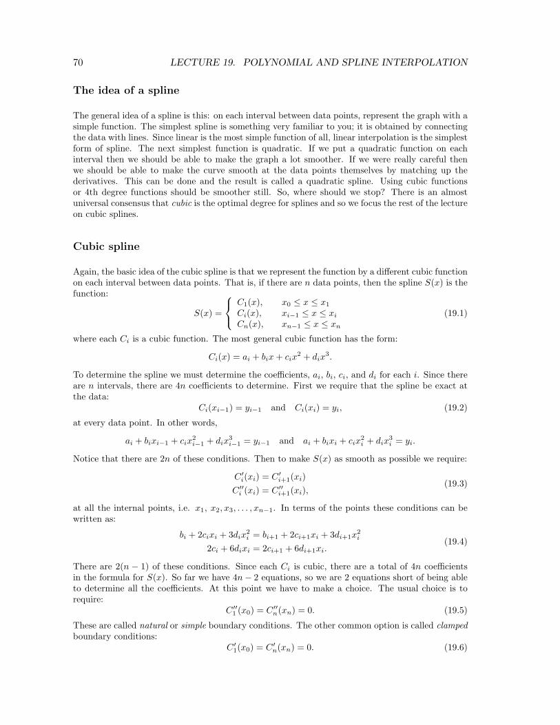
70 LECTURE 19. POLYNOMIAL AND SPLINE INTERPOLATION

The idea of a spline

The general idea of a spline is this: on each interval between data points, represent the graph with asimple function. The simplest spline is something very familiar to you; it is obtained by connectingthe data with lines. Since linear is the most simple function of all, linear interpolation is the simplestform of spline. The next simplest function is quadratic. If we put a quadratic function on eachinterval then we should be able to make the graph a lot smoother. If we were really careful thenwe should be able to make the curve smooth at the data points themselves by matching up thederivatives. This can be done and the result is called a quadratic spline. Using cubic functionsor 4th degree functions should be smoother still. So, where should we stop? There is an almostuniversal consensus that cubic is the optimal degree for splines and so we focus the rest of the lectureon cubic splines.

Cubic spline

Again, the basic idea of the cubic spline is that we represent the function by a different cubic functionon each interval between data points. That is, if there are n data points, then the spline S(x) is thefunction:

S(x) =

C1(x), x0 ≤ x ≤ x1

Ci(x), xi−1 ≤ x ≤ xi

Cn(x), xn−1 ≤ x ≤ xn

(19.1)

where each Ci is a cubic function. The most general cubic function has the form:

Ci(x) = ai + bix+ cix2 + dix

3.

To determine the spline we must determine the coefficients, ai, bi, ci, and di for each i. Since thereare n intervals, there are 4n coefficients to determine. First we require that the spline be exact atthe data:

Ci(xi−1) = yi−1 and Ci(xi) = yi, (19.2)

at every data point. In other words,

ai + bixi−1 + cix2i−1 + dix

3i−1 = yi−1 and ai + bixi + cix

2i + dix

3i = yi.

Notice that there are 2n of these conditions. Then to make S(x) as smooth as possible we require:

C ′i(xi) = C ′

i+1(xi)

C ′′i (xi) = C ′′

i+1(xi),(19.3)

at all the internal points, i.e. x1, x2, x3, . . . , xn−1. In terms of the points these conditions can bewritten as:

bi + 2cixi + 3dix2i = bi+1 + 2ci+1xi + 3di+1x

2i

2ci + 6dixi = 2ci+1 + 6di+1xi.(19.4)

There are 2(n − 1) of these conditions. Since each Ci is cubic, there are a total of 4n coefficientsin the formula for S(x). So far we have 4n− 2 equations, so we are 2 equations short of being ableto determine all the coefficients. At this point we have to make a choice. The usual choice is torequire:

C ′′1 (x0) = C ′′

n(xn) = 0. (19.5)

These are called natural or simple boundary conditions. The other common option is called clampedboundary conditions:

C ′1(x0) = C ′

n(xn) = 0. (19.6)

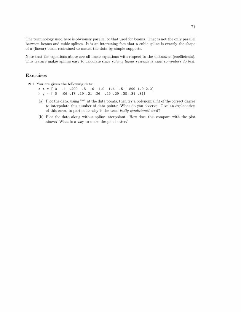
71

The terminology used here is obviously parallel to that used for beams. That is not the only parallelbetween beams and cubic splines. It is an interesting fact that a cubic spline is exactly the shapeof a (linear) beam restrained to match the data by simple supports.

Note that the equations above are all linear equations with respect to the unknowns (coefficients).This feature makes splines easy to calculate since solving linear systems is what computers do best.

Exercises

19.1 You are given the following data:> t = [ 0 .1 .499 .5 .6 1.0 1.4 1.5 1.899 1.9 2.0]

> y = [ 0 .06 .17 .19 .21 .26 .29 .29 .30 .31 .31]

(a) Plot the data, using ”*” at the data points, then try a polynomial fit of the correct degreeto interpolate this number of data points: What do you observe. Give an explanationof this error, in particular why is the term badly conditioned used?

(b) Plot the data along with a spline interpolant. How does this compare with the plotabove? What is a way to make the plot better?

Lecture 20

Least Squares Fitting: Noisy Data

Very often data has a significant amount of noise. The least squares approximation is intentionallywell-suited to represent noisy data. The next illustration shows the effects noise can have and howleast squares is used.

Traffic flow model

Suppose you are interested in the time it takes to travel on a certain section of highway for the sakeof planning. According to theory, assuming up to a moderate amount of traffic, the time should beapproximately:

T (x) = ax+ b

where b is the travel time when there is no other traffic, and x is the current number of cars on theroad (in hundreds). To determine the coefficients a and b you could run several experiments whichconsist of driving the highway at different times of day and also estimating the number of cars onthe road using a counter. Of course both of these measurements will contain noise, i.e. randomfluctuations.

We could simulate such data in Matlab as follows:> x = 1:.1:6;

> T = .1*x + 1;

> Tn = T + .1*randn(size(x));

> plot(x,Tn,’.’)

The data should look like it lies on a line, but with noise. Click on the Tools button and chooseBasic fitting. Then choose a linear fit. The resulting line should go through the data inwhat looks like a very reasonable way. Click on show equations. Compare the equation withT (x) = .1x+ 1. The coefficients should be pretty close considering the amount of noise in the plot.Next, try to fit the data with a spline. The result should be ugly. We can see from this examplethat splines are not suited to noisy data.

How does Matlab obtain a very nice line to approximate noisy data? The answer is a very standardnumerical/statistical method known as least squares.

Linear least squares

Consider in the previous example that we wish to fit a line to a lot of data that does not exactlylie on a line. For the equation of the line we have only two free coefficients, but we have many datapoints. We can not possibly make the line go through every data point, we can only wish for it tocome reasonably close to as many data points as possible. Thus, our line must have an error with

72

73

respect to each data point. If ℓ(x) is our line and (xi, yi) are the data, then

ei = yi − ℓ(xi)

is the error of ℓ with respect to each (xi, yi). To make ℓ(x) reasonable, we wish to simultaneouslyminimize all the errors: e1, e2, . . . , en. There are many possible ways one could go about this, butthe standard one is to try to minimize the sum of the squares of the errors. That is, we denote byE the sum of the squares:

E =

n∑

i=1

(yi − ℓ(xi))2=

n∑

i=1

(yi − axi − b)2. (20.1)

In the above expression xi and yi are given, but we are free to choose a and b, so we can think ofE as a function of a and b, i.e. E(a, b). In calculus, when one wishes to find a minimum value of afunction of two variables, we set the partial derivatives equal to zero:

∂E∂a

= −2n∑

i=1

(yi − axi − b)xi = 0

∂E∂b

= −2

n∑

i=1

(yi − axi − b) = 0.

(20.2)

We can simplify these equations to obtain:(

n∑

i=1

x2i

)

a+

(

n∑

i=1

xi

)

b =

n∑

i=1

xiyi

(

n∑

i=1

xi

)

a+ nb =n∑

i=1

yi.

(20.3)

Thus, the whole problem reduces to a 2 by 2 linear system to find the coefficients a and b. Theentries in the matrix are determined from simple formulas using the data. The process is quick andeasily automated, which is one reason it is very standard.

We could use the same process to obtain a quadratic or higher polynomial fit to data. If we try tofit an n degree polynomial, the software has to solve an n × n linear system, which is easily done.This is what Matlab’s basic fitting tool uses to obtain an n degree polynomial fit whenever thenumber of data points is more than n+ 1.

Drag coefficients

Drag due to air resistance is proportional to the square of the velocity, i.e. d = kv2. In a windtunnel experiment the velocity v can be varied by setting the speed of the fan and the drag can bemeasured directly (it is the force on the object). In this and every experiment some random noisewill occur. The following sequence of commands replicates the data one might receive from a windtunnel:> v = 0:1:60;

> d = .1234*v.^2;

> dn = d + .4*v.*randn(size(v));

> plot(v,dn,’*’)

The plot should look like a quadratic, but with some noise. Using the tools menu, add a quadraticfit and enable the “show equations” option. What is the coefficient of x2? How close is it to 0.1234?

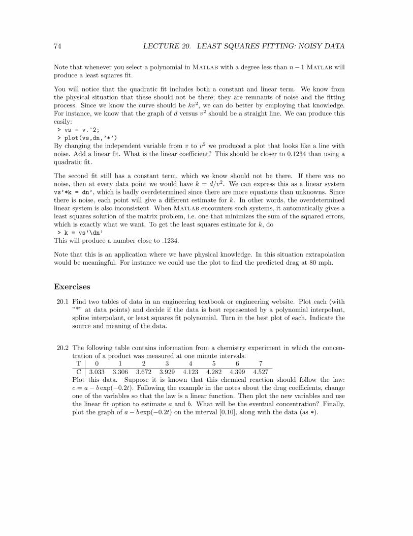
74 LECTURE 20. LEAST SQUARES FITTING: NOISY DATA

Note that whenever you select a polynomial in Matlab with a degree less than n− 1 Matlab willproduce a least squares fit.

You will notice that the quadratic fit includes both a constant and linear term. We know fromthe physical situation that these should not be there; they are remnants of noise and the fittingprocess. Since we know the curve should be kv2, we can do better by employing that knowledge.For instance, we know that the graph of d versus v2 should be a straight line. We can produce thiseasily:> vs = v.^2;

> plot(vs,dn,’*’)

By changing the independent variable from v to v2 we produced a plot that looks like a line withnoise. Add a linear fit. What is the linear coefficient? This should be closer to 0.1234 than using aquadratic fit.

The second fit still has a constant term, which we know should not be there. If there was nonoise, then at every data point we would have k = d/v2. We can express this as a linear systemvs’*k = dn’, which is badly overdetermined since there are more equations than unknowns. Sincethere is noise, each point will give a different estimate for k. In other words, the overdeterminedlinear system is also inconsistent. When Matlab encounters such systems, it automatically gives aleast squares solution of the matrix problem, i.e. one that minimizes the sum of the squared errors,which is exactly what we want. To get the least squares estimate for k, do> k = vs’\dn’

This will produce a number close to .1234.

Note that this is an application where we have physical knowledge. In this situation extrapolationwould be meaningful. For instance we could use the plot to find the predicted drag at 80 mph.

Exercises

20.1 Find two tables of data in an engineering textbook or engineering website. Plot each (with”*” at data points) and decide if the data is best represented by a polynomial interpolant,spline interpolant, or least squares fit polynomial. Turn in the best plot of each. Indicate thesource and meaning of the data.

20.2 The following table contains information from a chemistry experiment in which the concen-tration of a product was measured at one minute intervals.T 0 1 2 3 4 5 6 7C 3.033 3.306 3.672 3.929 4.123 4.282 4.399 4.527

Plot this data. Suppose it is known that this chemical reaction should follow the law:c = a− b exp(−0.2t). Following the example in the notes about the drag coefficients, changeone of the variables so that the law is a linear function. Then plot the new variables and usethe linear fit option to estimate a and b. What will be the eventual concentration? Finally,plot the graph of a− b exp(−0.2t) on the interval [0,10], along with the data (as *).

Lecture 21

Integration: Left, Right and TrapezoidRules

The Left and Right endpoint rules

In this section, we wish to approximate a definite integral:∫ b

a

f(x) dx

where f(x) is a continuous function. In calculus we learned that integrals are (signed) areas and canbe approximated by sums of smaller areas, such as the areas of rectangles. We begin by choosingpoints xi that subdivide [a, b]:

a = x0 < x1 < . . . < xn−1 < xn = b.

The subintervals [xi−1, xi] determine the width ∆xi of each of the approximating rectangles. Forthe height, we learned that we can choose any height of the function f(x∗

i ) where x∗i ∈ [xi−1, xi].

The resulting approximation is:

∫ b

a

f(x) dx ≈n∑

i=1

f(x∗i )∆xi.

To use this to approximate integrals with actual numbers, we need to have a specific x∗i in each

interval. The two simplest (and worst) ways to choose x∗i are as the left-hand point or the right-hand

point of each interval. This gives concrete approximations which we denote by Ln and Rn given by

Ln =

n∑

i=1

f(xi−1)∆xi and

Rn =

n∑

i=1

f(xi)∆xi .

function L = myleftsum(x,y)

% produces the left sum from data input.

% Inputs: x -- vector of the x coordinates of the partition

% y -- vector of the corresponding y coordinates

% Output: returns the approximate integral

n = max(size(x)); % safe for column or row vectors

L = 0;

for i = 1:n-1

L = L + y(i)*(x(i+1) - x(i));

end

75

76 LECTURE 21. INTEGRATION: LEFT, RIGHT AND TRAPEZOID RULES

-

6

-

6

Figure 21.1: The left and right sums, Ln and Rn.

Often we can take xi to be evenly spaced, with each interval having the same width:

h =b− a

n,

where n is the number of subintervals. If this is the case, then Ln and Rn simplify to:

Ln =b− a

n

n−1∑

i=0

f(xi) and (21.1)

Rn =b− a

n

n∑

i=1

f(xi). (21.2)

The foolishness of choosing left or right endpoints is illustrated in Figure 21.1. As you can see, fora very simple function like f(x) = 1+ .5x, each rectangle of Ln is too short, while each rectangle ofRn is too tall. This will hold for any increasing function. For decreasing functions Ln will alwaysbe too large while Rn will always be too small.

The Trapezoid rule

Knowing that the errors of Ln and Rn are of opposite sign, a very reasonable way to get a betterapproximation is to take an average of the two. We will call the new approximation Tn:

Tn =Ln +Rn

2.

This method also has a straight-forward geometric interpretation. On each subrectangle we areusing:

Ai =f(xi−1) + f(xi)

2∆xi ,

which is exactly the area of the trapezoid with sides f(xi−1) and f(xi). We thus call the methodthe trapezoid method. See Figure 21.2.

We can rewrite Tn as

Tn =

n∑

i=1

f(xi−1) + f(xi)

2∆xi.

77

-

6

HHHHH

HHHHH

Figure 21.2: The trapezoid rule, Tn.

In the evenly spaced case, we can write this as

Tn =b− a

2n

(

f(x0) + 2f(x1) + . . .+ 2f(xn−1) + f(xn))

. (21.3)

Caution: The convention used here is to begin numbering the points at 0, i.e. x0 = a; this allows nto be the number of subintervals and the index of the last point xn. However, Matlab’s indexingconvention begins at 1. Thus, when programming in Matlab, the first entry in x will be x0,i.e. x(1)= x0 and x(n+1)= xn.

If we are given data about the function, rather than a formula for the function, often the data arenot evenly spaced. The following function program could then be used.

function T = mytrap(x,y)

% Calculates the Trapezoid rule approximation of the integral from input data

% Inputs: x -- vector of the x coordinates of the partitian

% y -- vector of the corresponding y coordinates

% Output: returns the approximate integral

n = max(size(x)); % safe for column or row vectors

T = 0;

for i = 1:n-1

T = T + .5*(y(i)+y(i+1))*(x(i+1) - x(i));

end

Using the Trapezoid rule for areas in the plane

In multi-variable calculus you were supposed to learn that you can calculate the area of a region Rin the plane by calculating the line integral:

A = −∮

C

y dx, (21.4)

where C is the counter-clockwise curve around the boundary of the region. We can represent such acurve by consecutive points on it, i.e. x = (x0, x1, x2, . . . , xn−1, xn), and y = (y0, y1, y2, . . . , yn−1, yn).

78 LECTURE 21. INTEGRATION: LEFT, RIGHT AND TRAPEZOID RULES

Since we are assuming the curve ends where it begins, we require (xn, yn) = (x0, y0). Applying thetrapezoid method to the integral (21.4) gives

A = −n∑

i=1

yi−1 + yi2

(xi − xi−1).

This formula then is the basis for calculating areas when coordinates of boundary points are known,but not necessarily formulas for the boundaries such as in a land survey.

In the following script, we can use this method to approximate the area of a unit circle using npoints on the circle:

% Calculates pi using a trapezoid approximation of the unit circle.

format long

n = 10;

t = linspace(0,2*pi,n+1);

x = cos(t);

y = sin(t);

plot(x,y)

A = 0

for i = 1:n

A = A - (y(i)+y(i+1))*(x(i+1)-x(i))/2;

end

A

Exercises

21.1 For the integral∫ 2

1

√x dx calculate L4, R4, and T4 with even spacing (by hand, but use

a calculator) using formulas (21.1), (21.2) and (21.3). Find the percentage error of theseapproximations, using the exact value.

21.2 Write a function program myints whose inputs are f , a, b and n and whose outputs are L, Rand T , the left, right and trapezoid integral approximations for f on [a, b] with n subintervals.To make it efficient, use x = linspace(a,b,n+1) to make the x values and y = f(x) to makethe y values, add the 2nd to nth y entries once, and then add on the missing terms to obtainthe left, right and trapezoid approximations.

Change to format long and apply your program to the integral∫ 2

1

√x dx. Compare with the

results of the previous exercise. Also find L100, R100 and T100 and the relative errors of theseapproximations.

Turn in the program and a brief summary of the results.

Lecture 22

Integration: Midpoint and Simpson’sRules

Midpoint rule

If we use the endpoints of the subintervals to approximate the integral, we run the risk that the valuesat the endpoints do not accurately represent the average value of the function on the subinterval. Apoint which is much more likely to be close to the average would be the midpoint of each subinterval.Using the midpoint in the sum is called the midpoint rule. On the i-th interval [xi−1, xi] we will callthe midpoint xi, i.e.

xi =xi−1 + xi

2.

If ∆xi = xi − xi−1 is the length of each interval, then using midpoints to approximate the integralwould give the formula:

Mn =n∑

i=1

f(xi)∆xi .

For even spacing, ∆x = (b− a)/n, and the formula is:

Mn =b− a

n

n∑

i=1

f(xi) =b− a

n(y1 + y2 + . . .+ yn), (22.1)

where we define yi = f(xi).

While the midpoint method is obviously better than Ln or Rn, it is not obvious that it is actuallybetter than the trapezoid method Tn, but it is.

Simpson’s rule

Consider Figure 22.1. If f is not linear on a subinterval, then it can be seen that the errors forthe midpoint and trapezoid rules behave in a very predictable way, they have opposite sign. Forexample, if the function is concave up then Tn will be too high, while Mn will be too low. Thus itmakes sense that a better estimate would be to average Tn and Mn. However, in this case we cando better than a simple average. The error will be minimized if we use a weighted average. To findthe proper weight we take advantage of the fact that for a quadratic function the errors EMn andETn are exactly related by:

|EMn| =1

2|ETn| .

79

80 LECTURE 22. INTEGRATION: MIDPOINT AND SIMPSON’S RULES

-

6

u

Figure 22.1: Comparing the trapezoid and midpoint method on a single subinterval. Thefunction is concave up, in which case Tn is too high, while Mn is too low.

Thus we take the following weighted average of the two, which is called Simpson’s rule:

S2n =2

3Mn +

1

3Tn .

If we use this weighting on a quadratic function the two errors will exactly cancel.

Notice that we write the subscript as 2n. That is because we usually think of 2n subintervals in theapproximation; the n subintervals of the trapezoid are further subdivided by the midpoints. We canthen number all the points using integers. If we number them this way we notice that the numberof subintervals must be an even number.

The formula for Simpson’s rule if the subintervals are evenly spaced is the following (with n intervals,where n is even):

Sn =b− a

3n(f(x0) + 4f(x1) + 2f(x2) + 4f(x3) + . . .+ 2f(xn−2) + 4f(xn−1) + f(xn)) .

Note that if we are presented with data xi, yi where the xi points are evenly spaced with xi+1−xi =∆x, it is easy to apply Simpson’s method:

Sn =∆x

3(y0 + 4y1 + 2y2 + 4y3 + . . .+ 2yn−2 + 4yn−1 + yn) . (22.2)

Notice the pattern of the coefficients. The following program will produce these coefficients for nintervals, if n is an even number. Try it for n = 6, 7, 100.

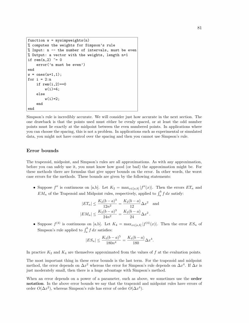
81

function w = mysimpweights(n)

% computes the weights for Simpson’s rule

% Input: n -- the number of intervals, must be even

% Output: a vector with the weights, length n+1

if rem(n,2) ~= 0

error(’n must be even’)

end

w = ones(n+1,1);

for i = 2:n

if rem(i,2)==0

w(i)=4;

else

w(i)=2;

end

end

Simpson’s rule is incredibly accurate. We will consider just how accurate in the next section. Theone drawback is that the points used must either be evenly spaced, or at least the odd numberpoints must lie exactly at the midpoint between the even numbered points. In applications whereyou can choose the spacing, this is not a problem. In applications such as experimental or simulateddata, you might not have control over the spacing and then you cannot use Simpson’s rule.

Error bounds

The trapezoid, midpoint, and Simpson’s rules are all approximations. As with any approximation,before you can safely use it, you must know how good (or bad) the approximation might be. Forthese methods there are formulas that give upper bounds on the error. In other words, the worstcase errors for the methods. These bounds are given by the following statements:

• Suppose f ′′ is continuous on [a,b]. Let K2 = maxx∈[a,b] |f ′′(x)|. Then the errors ETn and

EMn of the Trapezoid and Midpoint rules, respectively, applied to∫ b

af dx satisfy:

|ETn| ≤K2(b− a)3

12n2=

K2(b− a)

12∆x2 and

|EMn| ≤K2(b− a)3

24n2=

K2(b− a)

24∆x2 .

• Suppose f (4) is continuous on [a,b]. Let K4 = maxx∈[a,b] |f (4)(x)|. Then the error ESn of

Simpson’s rule applied to∫ b

af dx satisfies:

|ESn| ≤K4(b− a)5

180n4=

K4(b− a)

180∆x4.

In practice K2 and K4 are themselves approximated from the values of f at the evaluation points.

The most important thing in these error bounds is the last term. For the trapezoid and midpointmethod, the error depends on ∆x2 whereas the error for Simpson’s rule depends on ∆x4. If ∆x isjust moderately small, then there is a huge advantage with Simpson’s method.

When an error depends on a power of a parameter, such as above, we sometimes use the ordernotation. In the above error bounds we say that the trapezoid and midpoint rules have errors oforder O(∆x2), whereas Simpson’s rule has error of order O(∆x4).

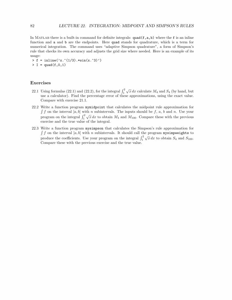
82 LECTURE 22. INTEGRATION: MIDPOINT AND SIMPSON’S RULES

In Matlab there is a built-in command for definite integrals: quad(f,a,b) where the f is an inlinefunction and a and b are the endpoints. Here quad stands for quadrature, which is a term fornumerical integration. The command uses “adaptive Simpson quadrature”, a form of Simpson’srule that checks its own accuracy and adjusts the grid size where needed. Here is an example of itsusage:> f = inline(’x.^(1/3).*sin(x.^3)’)

> I = quad(f,0,1)

Exercises

22.1 Using formulas (22.1) and (22.2), for the integral∫ 2

1

√x dx calculate M4 and S4 (by hand, but

use a calculator). Find the percentage error of these approximations, using the exact value.Compare with exercise 21.1.

22.2 Write a function program mymidpoint that calculates the midpoint rule approximation for∫

f on the interval [a, b] with n subintervals. The inputs should be f , a, b and n. Use your

program on the integral∫ 2

1

√x dx to obtain M4 and M100. Compare these with the previous

exercise and the true value of the integral.

22.3 Write a function program mysimpson that calculates the Simpson’s rule approximation for∫

f on the interval [a, b] with n subintervals. It should call the program mysimpweights to

produce the coefficients. Use your program on the integral∫ 2

1

√x dx to obtain S4 and S100.

Compare these with the previous exercise and the true value.

Lecture 23

Plotting Functions of Two Variables

Functions on Rectangular Grids

Suppose you wish to plot a function f(x, y) on the rectangle a ≤ x ≤ b and c ≤ y ≤ d. The graphof a function of two variables is of course a three dimensional object. Visualizing the graph is oftenvery useful.

For example, suppose you have a formula:

f(x, y) = x sin(xy)

and you are interested in the function on the region 0 ≤ x ≤ 5, π ≤ y ≤ 2π. A way to plot thisfunction in Matlab would be the following sequence of commands:> f = inline(’x.*sin(x.*y)’,’x’,’y’)

> [X,Y] = meshgrid(0:.1:5,pi:.01*pi:2*pi);

> Z = f(X,Y)

> mesh(X,Y,Z)

This will produce a 3-D plot that you can rotate by clicking on the rotate icon and then draggingwith the mouse.

Instead of the command mesh, you could use the command:> surf(X,Y,Z)

The key command in this sequence is [X Y] = meshgrid(a:h:b,c:k:d), which produces matricesof x and y values in X and Y. Enter:> size(X)

> size(Y)

> size(Z)

to see that each of these variables is a 101× 51 matrix. To see the first few entries of X enter:> X(1:6,1:6)

and to see the first few values of Y type:> Y(1:6,1:6)

You should observe that the x values in X begin at 0 on the left column and increase from left toright. The y values on the other have start at π at the top and increase from top to bottom. Notethat this arrangement is flipped from the usual arrangment in the x-y plane.

In the command [X Y] = meshgrid(a:h:b,c:k:d), h is the increment in the x direction and k isthe increment in the y direction. Often we will calculate:

h =b− a

mand k =

d− c

n,

where m is the number of intervals in the x direction and n is the number of intervals in the ydirection. To obtain a good plot it is best if m and n can be set between 10 and 100.

83

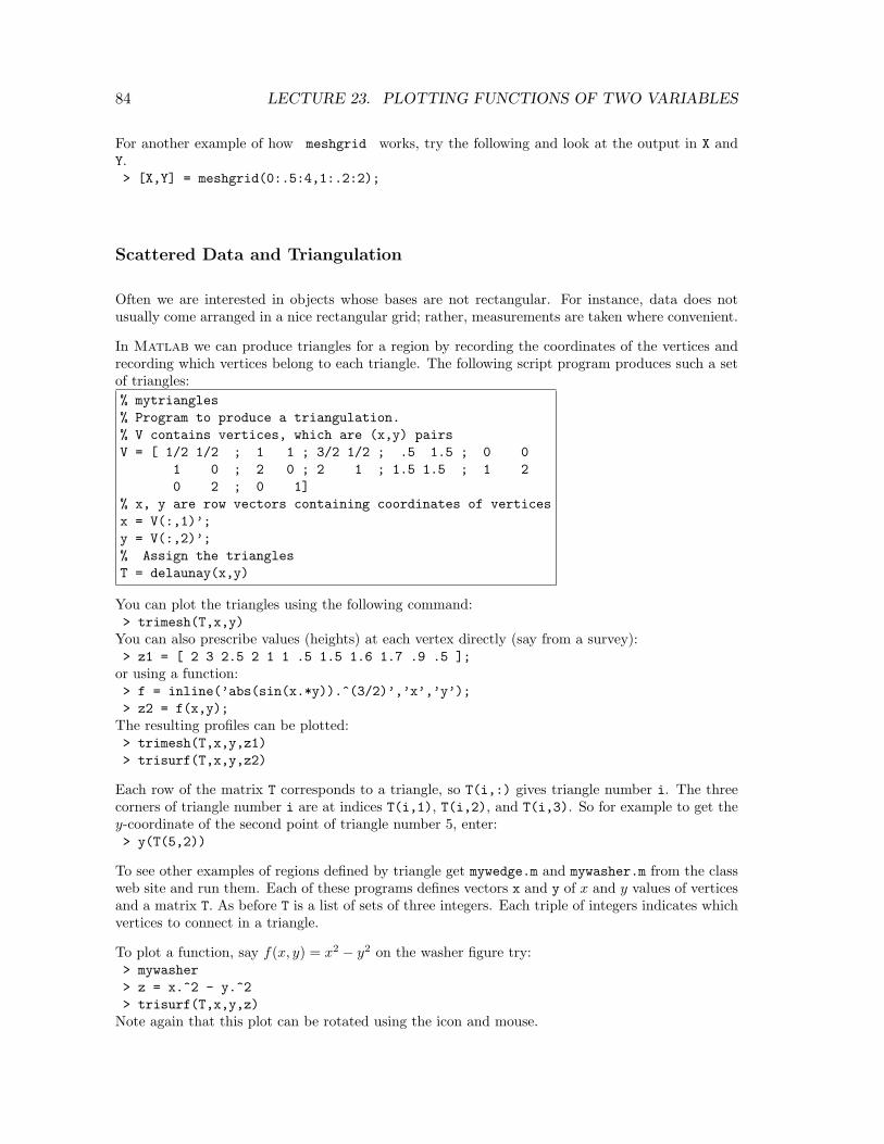
84 LECTURE 23. PLOTTING FUNCTIONS OF TWO VARIABLES

For another example of how meshgrid works, try the following and look at the output in X andY.> [X,Y] = meshgrid(0:.5:4,1:.2:2);

Scattered Data and Triangulation

Often we are interested in objects whose bases are not rectangular. For instance, data does notusually come arranged in a nice rectangular grid; rather, measurements are taken where convenient.

In Matlab we can produce triangles for a region by recording the coordinates of the vertices andrecording which vertices belong to each triangle. The following script program produces such a setof triangles:

% mytriangles

% Program to produce a triangulation.

% V contains vertices, which are (x,y) pairs

V = [ 1/2 1/2 ; 1 1 ; 3/2 1/2 ; .5 1.5 ; 0 0

1 0 ; 2 0 ; 2 1 ; 1.5 1.5 ; 1 2

0 2 ; 0 1]

% x, y are row vectors containing coordinates of vertices

x = V(:,1)’;

y = V(:,2)’;

% Assign the triangles

T = delaunay(x,y)

You can plot the triangles using the following command:> trimesh(T,x,y)

You can also prescribe values (heights) at each vertex directly (say from a survey):> z1 = [ 2 3 2.5 2 1 1 .5 1.5 1.6 1.7 .9 .5 ];

or using a function:> f = inline(’abs(sin(x.*y)).^(3/2)’,’x’,’y’);

> z2 = f(x,y);

The resulting profiles can be plotted:> trimesh(T,x,y,z1)

> trisurf(T,x,y,z2)

Each row of the matrix T corresponds to a triangle, so T(i,:) gives triangle number i. The threecorners of triangle number i are at indices T(i,1), T(i,2), and T(i,3). So for example to get they-coordinate of the second point of triangle number 5, enter:> y(T(5,2))

To see other examples of regions defined by triangle get mywedge.m and mywasher.m from the classweb site and run them. Each of these programs defines vectors x and y of x and y values of verticesand a matrix T. As before T is a list of sets of three integers. Each triple of integers indicates whichvertices to connect in a triangle.

To plot a function, say f(x, y) = x2 − y2 on the washer figure try:> mywasher

> z = x.^2 - y.^2

> trisurf(T,x,y,z)

Note again that this plot can be rotated using the icon and mouse.

85

Exercises

23.1 Plot the function f(x, y) = xe−x2−y2

on the rectangle −3 ≤ x ≤ 3, −2 ≤ y ≤ 2 usingmeshgrid. Make an appropriate choice of h and k and if necessary a rotation to produce agood plot. Turn in your plot and the calculation of k and h.

Lecture 24

Double Integrals for Rectangles

The center point method

Suppose that we need to find the integral of a function, f(x, y), on a rectangle:

R = (x, y) : a ≤ x ≤ b, c ≤ y ≤ d.

In calculus you learned to do this by an iterated integral:

I =

∫∫

R

f dA =

∫ b

a

∫ d

c

f(x, y) dydx =

∫ d

c

∫ b

a

f(x, y) dxdy.

You also should have learned that the integral is the limit of the Riemann sums of the function asthe size of the subrectangles goes to zero. This means that the Riemann sums are approximationsof the integral, which is precisely what we need for numerical methods.

For a rectangle R, we begin by subdividing into smaller subrectangles Rij, in a systematic way. Wewill divide [a, b] into m subintervals and [c, d] into n subintervals. Then Rij will be the “intersection”of the i-th subinterval in [a, b] with the j-th subinterval of [c, d]. In this way the entire rectangle issubdivided into mn subrectangles, numbered as in Figure 24.1.

A Riemann sum using this subdivision would have the form:

S =

m,n∑

i,j=1,1

f(x∗ij)Aij =

n∑

j=1

(

m∑

i=1

f(x∗ij)Aij

)

,

a bc

d

R11 R21 R31 R41

R12

R13

R14

R15

Figure 24.1: Subdivision of the rectangle R = [a, b]× [c, d] into subrectangles Rij .

86

87

where Aij = ∆xi∆yj is the area of Rij , and x∗ij is a point in Rij . The theory of integrals tells us

that if f is continuous, then this sum will converge to the same number, no matter how we choosex∗ij . For instance, we could choose x∗

ij to be the point in the lower left corner of Rij and the sumwould still converge as the size of the subrectangles goes to zero. However, in practice we wish tochoose x∗

ij in such a way to make S as accurate as possible even when the subrectangles are not verysmall. The obvious choice for the best point in Rij would be the center point. The center point ismost likely of all points to have a value of f close to the average value of f . If we denote the centerpoints by cij , then the sum becomes

Cmn =

m,n∑

i,j=1,1

f(cij)Aij .

Here

cij =

(

xi−1 + xi

2,yi−1 + yi

2

)

.

Note that if the subdivision is evenly spaced then ∆x ≡ (b − a)/m and ∆y ≡ (d − c)/n, and so inthat case

Cmn =(b− a)(d− c)

mn

m,n∑

i,j=1,1

f(cij).

The four corners method

Another good idea would be to take the value of f not only at one point, but as the average of thevalues at several points. An obvious choice would be to evaluate f at all four corners of each Rij

then average those. If we note that the lower left corner is (xi, yj), the upper left is (xi, yj+1), thelower right is (xi+1, yi) and the upper right is (xi+1, yi+1), then the corresponding sum will be

Fmn =

m,n∑

i,j=1,1

1

4(f(xi, yj) + f(xi, yj+1) + f(xi+1, yi) + f(xi+1, yj+1))Aij ,

which we will call the four-corners method. If the subrectangles are evenly spaced, then we cansimplify this expression. Notice that f(xi, yj) gets counted multiple times depending on where(xi, yj) is located. For instance if (xi, yj) is in the interior of R then it is the corner of 4 subrectangles.Thus the sum becomes

Fmn =A

4

∑

corners

f(xi, yj) + 2∑

edges

f(xi, yj) + 4∑

interior

f(xi, yj)

,

where A = ∆x∆y is the area of the subrectangles. We can think of this as a weighted average ofthe values of f at the grid points (xi, yj). The weights used are represented in the matrix

W =

1 2 2 2 · · · 2 2 12 4 4 4 · · · 4 4 22 4 4 4 · · · 4 4 2...

......

... · · ·...

......

2 4 4 4 · · · 4 4 21 2 2 2 · · · 2 2 1

. (24.1)

We could implement the four-corner method by forming a matrix (fij) of f values at the grid points,then doing entry-wise multiplication of the matrix with the weight matrix. Then the integral would

88 LECTURE 24. DOUBLE INTEGRALS FOR RECTANGLES

be obtained by summing all the entries of the resulting matrix and multiplying that by A/4. Theformula would be

Fmn =(b− a)(d− c)

4mn

m+1,n+1∑

i,j=1,1

Wijf(xi, yj).

Notice that the four-corners method coincides with applying the trapezoid rule in each direction.Thus it is in fact a double trapezoid rule.

The double Simpson method

The next improvement one might make would be to take an average of the center point sum Cmn

and the four corners sum Fmn. However, a more standard way to obtain a more accurate methodis the Simpson double integral. It is obtained by applying Simpson’s rule for single integrals to theiterated double integral. The resulting method requires that both m and n be even numbers andthe grid be evenly spaced. If this is the case we sum up the values f(xi, yj) with weights representedin the matrix

W =

1 4 2 4 · · · 2 4 14 16 8 16 · · · 8 16 42 8 4 8 · · · 4 8 24 16 8 16 · · · 8 16 4...

......

... · · ·...

......

2 8 4 8 · · · 4 8 24 16 8 16 · · · 8 16 41 4 2 4 · · · 2 4 1

. (24.2)

The sum of the weighted values is multiplied by A/9 and the formula is

Smn =(b− a)(d− c)

9mn

m+1,n+1∑

i,j=1,1

Wijf(xi, yj).

Matlab has a built in command for double integrals on rectangles: dblquad(f,a,b,c,d). Here isan example:> f = inline(’sin(x.*y)./sqrt(x+y)’,’x’,’y’)

> I = dblquad(f,0.5,1,0.5,2)

Below is a Matlab function which will produce the matrix of weights needed for Simpson’s rule fordouble integrals. It uses the function mysimpweights from Lecture 22.

function W = mydblsimpweights(m,n)

% Produces the m by n matrix of weights for Simpson’s rule

% for double integrals

% Inputs: m -- number of intervals in the row direction.

% must be even.

% n -- number of intervals in the column direction.

% must be even.

% Output: W -- a (m+1)x(n+1) matrix of the weights

if rem(m,2)~=0 | rem(n,2)~=0

error(’m and n must be even’)

end

u = mysimpweights(m);

v = mysimpweights(n);

W = u*v’;

89

Exercises

24.1 Download the program mylowerleft from the web site. Modify it to make a programmycenter that does the center point method. Implement the change by changing the “mesh-grid” to put the grid points at the centers of the subrectangles. Look at the mesh plot pro-duced to make sure the program is putting the grid where you want it. Use both programsto approximate the integral

∫ 2

0

∫ 5

1

√xy dy dx,

using (m,n) = (10, 18). Evaluate this integral exactly to make comparisons.

24.2 Write a program mydblsimp that computes the Simpson’s rule approximation. Let it call theprogram mydblsimpweights to make the weight matrix (24.2). Check the accuracy of theprogram on the integral in the previous problem.

24.3 Using mysimpweights and mydblsimpweights as models make programs mytrapweights andmydbltrapweights that will produce the weights for the trapezoid rule and the weight matrixfor the four corners (double trapezoid) method (24.1). Turn in the programs and the resultingweights for a 5× 6 grid.

Lecture 25

Double Integrals for Non-rectangles

In the previous lecture we considered only integrals over rectangular regions. In practice, regions ofinterest are rarely rectangles and so in this lecture we consider two strategies for evaluating integralsover other regions.

Redefining the function

One strategy is to redefine the function so that it is zero outside the region of interest, then integrateover a rectangle that includes the region.

For example, suppose we need to approximate the value of

I =

∫∫

T

sin3(xy) dx dy

where T is the triangle with corners at (0, 0), (1, 0) and (0, 2). Then we could let R be the rectangle[0, 1] × [0, 2] which contains the triangle T . Notice that the hypotenuse of the triangle has theequation 2x + y = 2. Then make f(x) = sin3(xy) if 2x + y ≤ 2 and f(x) = 0 if 2x + y > 2. InMatlab we can make this function with the command:> f = inline(’sin(x.*y).^3.*(2*x + y <= 2)’)

In this command <= is a logical command. The term in parentheses is then a logical statement andis given the value 1 if the statement is true and 0 if it is false. We can then integrate the modifiedf on [0, 1]× [0, 2] using the command:> I = dblquad(f,0,1,0,2)

As another example, suppose we need to integrate x2 exp(xy) inside the circle of radius 2 centeredat (1, 2). The equation for this circle is (x− 1)2 + (y − 2)2 = 4. Note that the inside of the circle is(x− 1)2 + (y− 2)2 ≤ 4 and that the circle is contained in the rectangle [−1, 3]× [0, 4]. Thus we cancreate the right function and integrate it by:> f = inline(’x.^2.*exp(x.*y).*((x-1).^2 + (y-2).^2 <= 4)’)

> I = dblquad(f,-1,3,0,4)

90

91

Integration Based on Triangles

The second approach to integrating over non-rectangular regions, is based on subdividing the regioninto triangles. Such a subdivision is called a triangulation. On regions where the boundary consistsof line segments, this can be done exactly. Even on regions where the boundary contains curves, thiscan be done approximately. This is a very important idea for several reasons, the most importantof which is that the finite elements method is based on it. Another reason this is important is thatoften the values of f are not given by a formula, but from data. For example, suppose you aresurveying on a construction site and you want to know how much fill will be needed to bring thelevel up to the plan. You would proceed by taking elevations at numerous points across the site.However, if the site is irregularly shaped or if there are obstacles on the site, then you cannot makethese measurements on an exact rectangular grid. In this case, you can use triangles by connectingyour points with triangles. Many software packages will even choose the triangles for you (Matlab

will do it using the command delaunay).

The basic idea of integrals based on triangles is exactly the same as that for rectangles; the integralis approximated by a sum where each term is a value times an area

I ≈n∑

i=1

f(x∗i )Ai ,

where n is the number of triangles, Ai is the area of the triangle and x∗ a point in the triangle.However, rather than considering the value of f at just one point people often consider an averageof values at several points. The most convenient of these is of course the corner points. We canrepresent this sum by

Tn =

n∑

i=1

fiAi ,

where f is the average of f at the corners.

If the triangle has vertices (x1, y1), (x2, y2) and (x3, y3), the formula for area is

A =1

2

∣

∣

∣

∣

∣

∣

det

x1 x2 x3

y1 y2 y31 1 1

∣

∣

∣

∣

∣

∣

. (25.1)

A function mythreecorners to compute using the three corners method is given below.

Another idea would be to use the center point (centroid) of each triangle. If the triangle has vertices(x1, y1), (x2, y2) and (x3, y3), then the centroid is given by the simple formulas

x =x1 + x2 + x3

3and y =

y1 + y2 + y33

. (25.2)

92 LECTURE 25. DOUBLE INTEGRALS FOR NON-RECTANGLES

function I = mythreecorners(f,V,T)

% Integrates a function based on a triangulation, using three corners

% Inputs: f -- the function to integrate, as an inline

% V -- the vertices. Each row has the x and y coordinates of a vertex

% T -- the triangulation. Each row gives the indices of three corners

% Output: the approximate integral

x = V(:,1); % extract x and y coordinates of all nodes

y = V(:,2);

I=0;

p = size(T,1);

for i = 1:p

x1 = x(T(i,1)); % find coordinates and area

x2 = x(T(i,2));

x3 = x(T(i,3));

y1 = y(T(i,1));

y2 = y(T(i,2));

y3 = y(T(i,3));

A = .5*abs(det([x1, x2, x3; y1, y2, y3; 1, 1, 1]));

z1 = f(x1,y1); % find values and average

z2 = f(x2,y2);

z3 = f(x3,y3);

zavg = (z1 + z2 + z3)/3;

I = I + zavg*A; % accumulate integral

end

Exercises

25.1 Download the programs mywedge.m and mywasher.m from the web site. Plot f(x, y) = x+yx2+y2

on the region produced by mywasher.m and f(x, y) = sin(x) +√y on the region produced by

mywedge.m.

25.2 Modify the program mythreecorners.m to a new program mycenters.m that does the cen-terpoint method for triangles. Run the program on the region produced by mywasher.m withthe function f(x, y) = x+y

x2+y2 and on the region produced by mywedge.m with the function

f(x, y) = sin(x) +√y.

Lecture 26

Gaussian Quadrature*

Exercises

26.1

26.2

93

Lecture 27

Numerical Differentiation

Approximating derivatives from data

Suppose that a variable y depends on another variable x, i.e. y = f(x), but we only know the valuesof f at a finite set of points, e.g., as data from an experiment or a simulation:

(x1, y1), (x2, y2), . . . , (xn, yn).

Suppose then that we need information about the derivative of f(x). One obvious idea would be toapproximate f ′(xi) by the Forward Difference:

f ′(xi) = y′i ≈yi+1 − yixi+1 − xi

.

This formula follows directly from the definition of the derivative in calculus. An alternative wouldbe to use a Backward Difference:

f ′(xi) ≈yi − yi−1

xi − xi−1.

Since the errors for the forward difference and backward difference tend to have opposite signs, itwould seem likely that averaging the two methods would give a better result than either alone. If thepoints are evenly spaced, i.e. xi+1 − xi = xi − xi−1 = h, then averaging the forward and backwarddifferences leads to a symmetric expression called the Central Difference:

f ′(xi) = y′i ≈yi+1 − yi−1

2h.

Errors of approximation

We can use Taylor polynomials to derive the accuracy of the forward, backward and central differenceformulas. For example the usual form of the Taylor polynomial with remainder (sometimes calledTaylor’s Theorem) is:

f(x+ h) = f(x) + hf ′(x) +h2

2f ′′(c),

where c is some (unknown) number between x and x+ h. Letting x = xi, x+ h = xi+1 and solvingfor f ′(xi) leads to:

f ′(xi) =f(xi+1)− f(xi)

h− h

2f ′′(c).

Notice that the quotient in this equation is exactly the forward difference formula. Thus the error ofthe forward difference is −(h/2)f ′′(c) which means it is O(h). Replacing h in the above calculation

94

95

−0.2 0 0.2 0.4 0.6 0.8 1 1.2−0.2

0

0.2

0.4

0.6

0.8

1

x

y

backward differenceforward differencecentral difference

(xi,y

i)

(xi −1

,yi −1

)

(xi+1

,yi+1

)

Figure 27.1: The three difference approximations of y′i.

by −h gives the error for the backward difference formula; it is also O(h). For the central difference,the error can be found from the third degree Taylor polynomial with remainder:

f(xi+1) = f(xi + h) = f(xi) + hf ′(xi) +h2

2f ′′(xi) +

h3

3!f ′′′(c1) and

f(xi−1) = f(xi − h) = f(xi)− hf ′(xi) +h2

2f ′′(xi)−

h3

3!f ′′′(c2)

where xi ≤ c1 ≤ xi+1 and xi−1 ≤ c2 ≤ xi. Subtracting these two equations and solving for f ′(xi)leads to:

f ′(xi) =f(xi+1)− f(xi−1)

2h− h2

3!

f ′′′(c1) + f ′′′(c2)

2.

This shows that the error for the central difference formula is O(h2). Thus, central differences aresignificantly better and so: It is best to use central differences whenever possible.

There are also central difference formulas for higher order derivatives. These all have error of orderO(h2):

f ′′(xi) = y′′i ≈ yi+1 − 2yi + yi−1

h2,

f ′′′(xi) = y′′′i ≈ 1

2h3[yi+2 − 2yi+1 + 2yi−1 − yi−2] , and

f (4)(xi) = y(4)i ≈ 1

h4[yi+2 − 4yi+1 + 6yi − 4yi−1 + yi−2] .

Partial Derivatives

Suppose u = u(x, y) is a function of two variables that we only know at grid points (xi, yj). We willuse the notation:

ui,j = u(xi, yj)

96 LECTURE 27. NUMERICAL DIFFERENTIATION

frequently throughout the rest of the lectures. We can suppose that the grid points are evenlyspaced, with an increment of h in the x direction and k in the y direction. The central differenceformulas for the partial derivatives would be:

ux(xi, yj) ≈1

2h(ui+1,j − ui−1,j) and

uy(xi, yj) ≈1

2k(ui,j+1 − ui,j−1) .

The second partial derivatives are:

uxx(xi, yj) ≈1

h2(ui+1,j − 2ui,j + ui−1,j) and

uyy(xi, yj) ≈1

k2(ui,j+1 − 2ui,j + ui,j−1) ,

and the mixed partial derivative is:

uxy(xi, yj) ≈1

4hk(ui+1,j+1 − ui+1,j−1 − ui−1,j+1 + ui−1,j−1) .

Caution: Notice that we have indexed uij so that as a matrix each row represents the values ofu at a certain xi and each column contains values at yj . The arrangement in the matrix does notcoincide with the usual orientation of the xy-plane.

Let’s consider an example. Let the values of u at (xi, yj) be recorded in the matrix:

(uij) =

5.1 6.5 7.5 8.1 8.45.5 6.8 7.8 8.3 8.95.5 6.9 9.0 8.4 9.15.4 9.6 9.1 8.6 9.4

(27.1)

Assume the indices begin at 1, i is the index for rows and j the index for columns. Suppose thath = .5 and k = .2. Then uy(x2, y4) would be approximated by the central difference:

uy(x2, y4) ≈u2,5 − u2,3

2k≈ 8.9− 7.8

2 · 0.2 = 2.75.

The partial derivative uxy(x2, y4) is approximated by:

uxy(x2, y4) ≈u3,5 − u3,3 − u1,5 + u1,3

4hk≈ 9.1− 9.0− 8.4 + 7.5

4 · .5 · .2 = −2.

Exercises

27.1 Suppose you are given the data in the following table.t 0 .5 1.0 1.5 2.0y 0 .19 .26 .29 .31

a. Give the forward, backward and central difference approximations of f ′(1).b. Give the central difference approximations for f ′′(1), f ′′′(1) and f (4)(1).

27.2 Suppose values of u(x, y) at points (xi, yj) are given in the matrix (27.1). Suppose that h = .1and k = .5. Approximate the following derivatives by central differences:a. ux(x2, y4)b. uxx(x3, y2)c. uyy(x3, y2)d. uxy(x2, y3)

Lecture 28

The Main Sources of Error

Truncation Error

Truncation error is defined as the error caused directly by an approximation method. For instance,all numerical integration methods are approximations and so there is error, even if the calculationsare performed exactly. Numerical differentiation also has a truncation error, as will the differentialequations methods we will study in Part IV, which are based on numerical differentiation formulas.There are two ways to minimize truncation error: (1) use a higher order method, and (2) use afiner grid so that points are closer together. Unless the grid is very small, truncation errors areusually much larger than roundoff errors. The obvious tradeoff is that a smaller grid requires morecalculations, which in turn produces more roundoff errors and requires more running time.

Roundoff Error

Roundoff error always occurs when a finite number of digits are recorded after an operation. For-tunately, this error is extremely small. The standard measure of how small is called machineepsilon. It is defined as the smallest number that can be added to 1 to produce another numberon the machine, i.e. if a smaller number is added the result will be rounded down to 1. In IEEEstandard double precision (used by Matlab and most serious software), machine epsilon is 2−52

or about 2.2 × 10−16. A different, but equivalent, way of thinking about this is that the machinerecords 52 floating binary digits or about 15 floating decimal digits. Thus there are never more than15 significant digits in any calculation. This of course is more than adequate for any application.However, there are ways in which this very small error can cause problems.

To see an unexpected occurence of round-off try the following commands:> (2^52+1) - 2^52

> (2^53+1) - 2^53

Loss of Precision (also called Loss of Significance)

One way in which small roundoff errors can become more significant is when significant digits cancel.For instance, if you were to calculate:

1234567(1− .9999987654321)

then the result should be

1.52415678859930.

97

98 LECTURE 28. THE MAIN SOURCES OF ERROR

But, if you input:> 1234567 * ( 1 - .9999987654321)

you will get:> 1.52415678862573

In the correct calculation there are 15 significant digits, but the Matlab calculation has only 11significant digits.

Although this seems like a silly example, this type of loss of precision can happen by accident if youare not careful. For example in f ′(x) ≈ (f(x+ h)− f(x))/h you will lose precision when h gets toosmall. Try:

> format long

> format compact

> f=inline(’x^2’,’x’)

> for i = 1:30

> h=10^(-i)

> df=(f(1+h)-f(1))/h

> relerr=(2-df)/2

> end

At first the relative error decreases since truncation error is reduced. Then loss of precision takesover and the relative error increases to 1.

Bad Conditioning

We encountered bad conditioning in Part II, when we talked about solving linear systems. Badconditioning means that the problem is unstable in the sense that small input errors can producelarge output errors. This can be a problem in a couple of ways. First, the measurements used to getthe inputs cannot be completely accurate. Second, the computations along the way have roundofferrors. Errors in the computations near the beginning especially can be magnified by a factor closeto the condition number of the matrix. Thus what was a very small problem with roundoff canbecome a very big problem.

It turns out that matrix equations are not the only place where condition numbers occur. In anyproblem one can define the condition number as the maximum ratio of the relative errors in theoutput versus input, i.e.

condition # of a problem = max

(

Relative error of output

Relative error of inputs

)

.

An easy example is solving a simple equation:

f(x) = 0.

Suppose that f ′ is close to zero at the solution x∗. Then a very small change in f (caused perhapsby an inaccurate measurement of some of the coefficients in f) can cause a large change in x∗. Itcan be shown that the condition number of this problem is 1/f ′(x∗).

99

Exercises

28.1 Identify the (main) source of error in each case and propose a way to reduce this error ifpossible.

(a) If we do (√3)2 we should get 3, but if we check

> mythree=(sqrt(3))^2

> mythree-3

we find the error is ans=-4.4409e-16.

(b) Since it is a quarter of a circle of radius 2, we should have∫ 2

0

√4− x2dx = 1

4π22 = π.

We try to use mytrap from Lecture 21 and do> x=0:.2:2;

> y=sqrt(4-x.^2);

> mypi=mytrap(x,y)

> mypi-pi

and find the error is ans=-0.0371.

28.2 1 The function f(x) = (x − 2)9 could be evaluated as written, or first expanded as f(x) =x9 − 18x8 + · · · and then evaluated. To find the expanded version, type> syms x

> expand((x-2)^9)

> clear

To evaluate it the first way, type> f1=inline(’(x-2).^9’,’x’)

> x=1.92:.001:2.08;

> y1=f1(x);

> plot(x,y1,’blue’)

To do it the second way, convert the expansion above to an inline function f2 and then type> y2=f2(x);

> hold on

> plot(x,y2,’red’)

Carefully study the resulting graphs. Should the graphs be the same? Which is more correct?Matlab does calculations using approximately 16 decimal places. What is the largest error inthe graph, and how big is it relative to 10−16? Which source of error is causing this problem?

1From Numerical Linear Algebra by L. Trefethen and D. Baum, SIAM, 1997.

Review of Part III

Methods and Formulas

Polynomial Interpolation:An exact fit to the data.For n data points it is a n− 1 degree polynomial.Only good for very few, accurate data points.The coefficients are found by solving a linear system of equations.

Spline Interpolation:Fit a simple function between each pair of points.Joining points by line segments is the most simple spline.Cubic is by far the most common and important.Cubic matches derivatives and second derivatives at data points.Simply supported and clamped ends are available.Good for more, but accurate points.The coefficients are found by solving a linear system of equations.

Least Squares:Makes a “close fit” of a simple function to all the data.Minimizes the sum of the squares of the errors.Good for noisy data.The coefficients are found by solving a linear system of equations.

Interpolation vs. Extrapolation: Polynomials, Splines and Least Squares are generally used forInterpolation, fitting between the data. Extrapolation, i.e. making fits beyond the data, is muchmore tricky. To make predictions beyond the data, you must have knowledge of the underlyingprocess, i.e. what the function should be.

Numerical Integration:Left Endpoint:

Ln =

n∑

i=1

f(xi−1)∆xi

Right Endpoint:

Rn =

n∑

i=1

f(xi)∆xi.

Trapezoid Rule:

Tn =n∑

i=1

f(xi−1) + f(xi)

2∆xi.

Midpoint Rule:

Mn =

n∑

i=1

f(xi)∆xi where xi =xi−1 + xi

2.

100

101

Numerical Integration Rules with Even Spacing:For even spacing: ∆x = b−a

n where n is the number of subintervals, then:

Ln = ∆x

n−1∑

i=0

yi =b− a

n

n−1∑

i=0

f(xi),

Rn = ∆x

n∑

i=1

yi =b− a

n

n∑

i=1

f(xi),

Tn = ∆x(

y0 + 2y1 + . . .+ 2yn−1 + yn)

=b− a

2n

(

f(x0) + 2f(x1) + . . .+ 2f(xn−1) + f(xn))

,

Mn = ∆x

n∑

i=1

yi =b− a

n

n∑

i=1

f(xi),

Simpson’s rule:

Sn = ∆x(

y0 + 4y1 + 2y2 + 4y3 + . . .+ 2yn−2 + 4yn−1 + yn)

=b− a

3n(f(x0) + 4f(x1) + 2f(x2) + 4f(x3) + . . .+ 2f(xn−2) + 4f(xn−1) + f(xn)) .

Area of a region:

A = −∮

C

y dx,

where C is the counter-clockwise curve around the boundary of the region. We can represent such acurve, by consecutive points on it, i.e. x = (x0, x1, x2, . . . , xn−1, xn), and y = (y0, y1, y2, . . . , yn−1, yn)with (xn, yn) = (x0, y0). Applying the trapezoid method to the integral (21.4):

A = −n∑

i=1

yi−1 + yi2

(xi − xi−1)

Accuracy of integration rules:Right and Left endpoint are O(∆x)Trapezoid and Midpoint are O(∆x2)Simpson is O(∆x4)

Double Integrals on Rectangles:Centerpoint:

Cmn =

m,n∑

i,j=1,1

f(cij)Aij .

where

cij =

(

xi−1 + xi

2,yi−1 + yi

2

)

.

Centerpoint – Evenly spaced:

Cmn = ∆x∆y

m,n∑

i,j=1,1

zij =(b− a)(d− c)

mn

m,n∑

i,j=1,1

f(cij).

Four corners:

Fmn =

m,n∑

i,j=1,1

1

4(f(xi, yj) + f(xi, yj+1) + f(xi+1, yi) + f(xi+1, yj+1))Aij ,

102 REVIEW OF PART III

Four Corners – Evenly spaced:

Fmn =A

4

∑

corners

f(xi, yj) + 2∑

edges

f(xi, yj) + 4∑

interior

f(xi, yj)

=(b− a)(d− c)

4mn

m,n∑

i,j=1,1

Wijf(xi, yj).

where

W =

1 2 2 2 · · · 2 2 12 4 4 4 · · · 4 4 22 4 4 4 · · · 4 4 2...

......

... · · ·...

......

2 4 4 4 · · · 4 4 21 2 2 2 · · · 2 2 1

.

Double Simpson:

Smn =(b− a)(d− c)

9mn

m,n∑

i,j=1,1

Wijf(xi, yj).

where

W =

1 4 2 4 · · · 2 4 14 16 8 16 · · · 8 16 42 8 4 8 · · · 4 8 24 16 8 16 · · · 8 16 4...

......

... · · ·...

......

2 8 4 8 · · · 4 8 24 16 8 16 · · · 8 16 41 4 2 4 · · · 2 4 1

.

Integration based on triangles:– Triangulation: Dividing a region up into triangles.– Triangles are suitable for odd-shaped regions.– A triangulation is better if the triangles are nearly equilateral.Three corners:

Tn =n∑

i=1

fiAi

where f is the average of f at the corners of the i-th triangle.Area of a triangle with corners (x1, y1), (x2, y2), (x3, y3):

A =1

2

∣

∣

∣

∣

∣

∣

det

x1 x2 x3

y1 y2 y31 1 1

∣

∣

∣

∣

∣

∣

.

Centerpoint:

C =

n∑

i=1

f(xi, yi)Ai, with

x =x1 + x2 + x3

3and y =

y1 + y2 + y33

.

103

Forward Difference:

f ′(xi) = y′i ≈yi+1 − yixi+1 − xi

.

Backward Difference:

f ′(xi) ≈yi − yi−1

xi − xi−1.

Central Difference:

f ′(xi) = y′i ≈yi+1 − yi−1

2h.

Higher order central differences:

f ′′(xi) = y′′i ≈ yi+1 − 2yi + yi−1

h2,

f ′′′(xi) = y′′′i ≈ 1

2h3[yi+2 − 2yi+1 + 2yi−1 − yi−2] ,

f (4)(xi) = y(4)i ≈ 1

h4[yi+2 − 4yi+1 + 6yi − 4yi−1 + yi−2] .

Partial Derivatives: Denote ui,j = u(xi, yj).

ux(xi, yj) ≈1

2h(ui+1,j − ui−1,j) ,

uy(xi, yj) ≈1

2k(ui,j+1 − ui,j−1) ,

uxx(xi, yj) ≈1

h2(ui+1,j − 2ui,j + ui−1,j) ,

uyy(xi, yj) ≈1

k2(ui,j+1 − 2ui,j + ui,j−1) ,

uxy(xi, yj) ≈1

4hk(ui+1,j+1 − ui+1,j−1 − ui−1,j+1 + ui−1,j−1) .

Sources of error:Truncation – the method is an approximation.Roundoff – double precision arithmetic uses ≈ 15 significant digits.Loss of precision – an amplification of roundoff error due to cancellations.Bad conditioning – the problem is sensitive to input errors.Error can build up after multiple calculations.

Matlab

Data Interpolation:Use the plot command plot(x,y,’*’) to plot the data.Use the Basic Fitting tool to make an interpolation or spline.If you choose an n− 1 degree polynomial with n data points the result will be the exact polynomialinterpolation.If you select a polynomial degree less than n−1, then Matlab will produce a least squares approx-imation.

Integration> quadl(f,a,b) . . . . . . . . . . . . . . . . . . . . . . . . . . . . . . . . . . . . . . . . . . . . Numerical integral of f(x) on [a, b].

104 REVIEW OF PART III

> dblquad(f,a,b,c,d) . . . . . . . . . . . . . . . . . . . . . . . . . . . . . . . . . . . . . . Integral of f(x, y) on [a, b]× [c, d].Example:> f = inline(’sin(x.*y)/sqrt(x+y)’,’x’,’y’)

> I = dblquad(f,0,1,0,2)

Matlab uses an advanced form of Simpson’s method.

Integration over non-rectangles:Redefine the function to be zero outside the region. For example:

> f = inline(’sin(x.*y).^3.*(2*x + y <= 2)’)

> I = dblquad(f,0,1,0,2)

Integrates f(x, y) = sin3(xy) on the triangle with corners (0, 0), (0, 2), and (1, 0).

Triangles:Matlab stores triangulations as a matrix of vertices V and triangles T.> T = delaunay(V) (or delaunay(x,y )) . . . . . . . . . . . . . . . . . . . .Produces triangles from vertices.> trimesh(T,x,y)

> trimesh(T,x,y,z)

> trisurf(T,x,y)

> trisurf(T,x,y,z)

Part IV

Differential Equations

c©Copyright, Todd Young and Martin Mohlenkamp, Mathematics Department, Ohio University, 2007

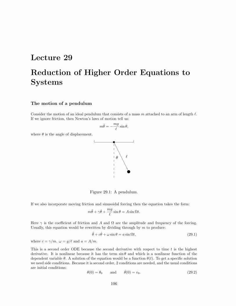
Lecture 29

Reduction of Higher Order Equations toSystems

The motion of a pendulum

Consider the motion of an ideal pendulum that consists of a mass m attached to an arm of length ℓ.If we ignore friction, then Newton’s laws of motion tell us:

mθ = −mg

ℓsin θ,

where θ is the angle of displacement.

tAAAAAAAAw

ℓθ

Figure 29.1: A pendulum.

If we also incorporate moving friction and sinusoidal forcing then the equation takes the form:

mθ + γθ +mg

ℓsin θ = A sinΩt.

Here γ is the coefficient of friction and A and Ω are the amplitude and frequency of the forcing.Usually, this equation would be rewritten by dividing through by m to produce:

θ + cθ + ω sin θ = a sinΩt, (29.1)

where c = γ/m. ω = g/ℓ and a = A/m.

This is a second order ODE because the second derivative with respect to time t is the highestderivative. It is nonlinear because it has the term sin θ and which is a nonlinear function of thedependent variable θ. A solution of the equation would be a function θ(t). To get a specific solutionwe need side conditions. Because it is second order, 2 conditions are needed, and the usual conditionsare initial conditions:

θ(0) = θ0 and θ(0) = v0. (29.2)

106

107

Converting a general higher order equation

All of the standard methods for solving ordinary differential equations are intended for first orderequations. For this reason, it is inconvenient to solve higher order equations numerically. However,most higher-order differential equations that occur in applications can be converted to a system offirst order equations and that is what is usually done in practice.

Suppose that an n-th order equation can be solved for the n-th derivative, i.e. it can be written inthe form:

x(n) = f

(

t, x, x, x, . . . ,dn−1x

dtn−1

)

. (29.3)

Then it can be converted to a first-order system by this standard change of variables:

y1 = x

y2 = x

...

yn = x(n−1) =dn−1x

dtn−1.

(29.4)

The resulting first-order system is the following:

y1 = x = y2

y2 = x = y3

...

yn = x(n) = f(t, y1, y2, . . . , yn).

(29.5)

In vector form this is simply y = f(t,y) with fi(t,y) = yi+1 for i < n and fn(t,y) = f(t, y1, y2, . . . , yn).

For the example of the pendulum (29.1) the change of variables has the form

y1 = θ

y2 = θ,(29.6)

and the resulting equations are

y1 = y2

y2 = −cy2 − ω sin(y1) + a sin(Ωt).(29.7)

In vector form this is

y =

(

y2−cy2 − ω sin(y1) + a sin(Ωt)

)

.

The initial conditions are converted to

y(0) =

(

y1(0)y2(0)

)

=

(

θ0v0

)

. (29.8)

As stated above, the main reason we wish to change a higher order equation into a system ofequations is that this form is convenient for solving the equation numerically. Most general softwarefor solving ODEs (including Matlab) requires that the ODE be input in the form of a first-ordersystem. In addition, there is a conceptual reason to make the change. In a system described by a

108 LECTURE 29. REDUCTION OF HIGHER ORDER EQUATIONS TO SYSTEMS

higher order equation, knowing the position is not enough to know what the system is doing. Inthe case of a second order equation, such as the pendulum, one must know both the angle and theangular velocity to know what the pendulum is really doing. We call the pair (θ, θ) the state of thesystem. Generally in applications the vector y is the state of the system described by the differentialequation.

Using Matlab to solve a system of ODE’s

In Matlab there are several commands that can be used to solve an initial value problem fora system of differential equations. Each of these correspond to different solving methods. Thestandard one to use is ode45, which uses the algorithm “Runge-Kutta 4 5”. We will learn aboutthis algorithm later.

To implement ode45 for a system, we have to input the vector function f that defines the system.For the pendulum system (29.7), we will assume that all the constants are 1, except c = .1, then wecan input the right hand side as:> f = inline(’[y(2);-.1*y(2)-sin(y(1))+sin(t)]’,’t’,’y’)

The command ode45 is then used as follows:> [T Y] = ode45(f,[0 20],[1;-1.5]);

Here [0 20] is the time span you want to consider and [1;-1.5] is the initial value of the vectory. The output T contains times and Y contains values of the vector y at those times. Try:> size(T)

> T(1:10)

> size(Y)

> Y(1:10,:)

Since the first coordinate of the vector is the position (angle), we are mainly interested in its values:> theta = Y(:,1);

> plot(T,theta)

In the next two sections we will learn enough about numerical methods for initial value problemsto understand roughly how Matlab produces this approximate solution.

Exercises

29.1 Consider the pendulum system but with no friction or forcing, i.e. γ = A = 0. What wouldbe equation (29.7) become in this case? Use the last example to solve the system with theinitial condition [θ0, 0]

′ for θ0 = .1π. Use the plot of the solution to find the frequency ofthe pendulum with this initial condition. Do the same for θ0 = .5pi and .9π. How does thefrequency depend on the amplitude of a pendulum?

29.2 Transform the given ODE into a first order system:

...x + x2 − 3x3 + cos2 x = e−t sin(3t).

Suppose the initial conditions for the ODE are: x(1) = 1, x(1) = 2, and x(1) = 0. Finda numerical solution of this IVP using ode45 and plot the first coordinate (x). Try timeintervals [1 2] and [1 2.1] and explain what you observe. (Remember to use entry-wiseoperations, .* and .^, in the definition of the vector function.)

Lecture 30

Euler Methods

Numerical Solution of an IVP

Suppose we wish to numerically solve the initial value problem

y = f(t,y), y(a) = y0, (30.1)

on an interval of time [a, b].

By a numerical solution, we must mean an approximation of the solution at a finite number ofpoints, i.e.

(t0,y0), (t1,y1), (t2,y2), . . . , (tn,yn),

where t0 = a and tn = b. The first of these points is exactly the initial value. If we take n steps asabove, and the steps are evenly spaced, then the time change in each step is

h =b− a

n, (30.2)

and the times ti are given simply by ti = a + ih. This leaves the most important part of finding anumerical solution: determining y1,y2, . . . ,yn in a way that is as consistent as possible with (30.1).To do this, first write the differential equation in the indexed notation

yi ≈ f(ti,yi), (30.3)

and will then replace the derivative y by a difference. There are many ways we might carry this outand in the next section we study the simplest.

The Euler Method

The most straight forward approach is to replace yi in (30.3) by its forward difference approximation.This gives

yi+1 − yi

h= f(ti,yi).

Rearranging this gives us a way to obtain yi+1 from yi known as Euler’s method:

yi+1 = yi + hf(ti,yi). (30.4)

With this formula, we can start from (t0,y0) and compute all the subsequent approximations (ti,yi).This is very easy to implement, as you can see from the following program (which can be downloadedfrom the class web site):

109

110 LECTURE 30. EULER METHODS

function [T , Y] = myeuler(f,tspan,y0,n)

% function [T , Y] = myeuler(f,tspan,y0,n)

% Solves dy/dt = f(t,y) with initial condition y(a) = y0

% on the interval [a,b] using n steps of Euler s method.

% Inputs: f -- a function f(t,y) that returns a column vector of the same

% length as y

% tspan -- a vector [a,b] with the start and end times

% y0 -- a column vector of the initial values, y(a) = y0

% n -- number of steps to use

% Outputs: T -- a n+1 column vector containing the times

% Y -- a (n+1) by d matrix where d is the length of y

% Y(t,i) gives the ith component of y at time t

% parse starting and ending points

a = tspan(1);

b = tspan(2);

h = (b-a)/n; % step size

t = a; y = y0; % t and y are the current variables

T = a; Y = y0’; % T and Y will record all steps

for i = 1:n

y = y + h*f(t,y);

t = a + i*h;

T = [T; t];

Y = [Y; y’];

end

To use this program we need a function, such as the vector function for the pendulum:> f = inline(’[y(2);-.1*y(2)-sin(y(1)) + sin(t)]’,’t’,’y’)

Then type:> [T Y] = myeuler(f,[0 20],[1;-1.5],5);

Here [0 20] is the time span you want to consider, [1;-1.5] is the initial value of the vector y and5 is the number of steps. The output T contains times and Y contains values of the vector as thetimes. Try:> size(T)

> size(Y)

Since the first coordinate of the vector is the angle, we only plot its values:> theta = Y(:,1);

> plot(T,theta)

In this plot it is clear that n = 5 is not adequate to represent the function. Type:> hold on

then redo the above with 5 replaced by 10. Next try 20, 40, 80, and 200. As you can see the graphbecomes increasingly better as n increases. We can compare these calculations with Matlab’sbuilt-in function with the commands:> [T Y]= ode45(f,[0 20],[1;-1.5]);

> theta = Y(:,1);

> plot(T,theta,’r’)

111

The problem with the Euler method

You can think of the Euler method as finding a linear approximate solution to the initial valueproblem on each time interval. An obvious shortcoming of the method is that it makes the approx-imation based on information at the beginning of the time interval only. This problem is illustratedwell by the following IVP:

x+ x = 0, x(0) = 1, x(0) = 0 . (30.5)

You can easily check that the exact solution of this IVP is

x(t) = cos(t).

If we make the standard change of variables

y1 = x, y2 = x,

then we get

y1 = y2, y2 = −y1.

Then the solution should be y1(t) = cos(t), y2(t) = sin(t). If we then plot the solution in the (y1, y2)plane, we should get exactly a unit circle. We can solve this IVP with Euler’s method:> g = inline(’[y(2);-y(1)]’,’t’,’y’)

> [T Y] = myeuler(g,[0 4*pi],[1;0],20)

> y1 = Y(:,1);

> y2 = Y(:,2);

> plot(y1,y2)

As you can see the approximate solution goes far from the true solution. Even if you increase thenumber of steps, the Euler solution will eventually drift outward away from the circle because itdoes not take into account the curvature of the solution.

The Modified Euler Method

An idea which is similar to the idea behind the trapezoid method would be to consider f at boththe beginning and end of the time step and take the average of the two. Doing this produces theModified (or Improved) Euler method represented by the following equations:

k1 = hf(ti,yi)

k2 = hf(ti + h,yi + k1)

yi+1 = yi +1

2(k1 + k2) .

(30.6)

Here k1 captures the information at the beginning of the time step (same as Euler), while k2 is theinformation at the end of the time step.

The following program implements the Modified method. It may be downloaded from the class website.

112 LECTURE 30. EULER METHODS

function [T , Y] = mymodeuler(f,tspan,y0,n)

% Solves dy/dt = f(t,y) with initial condition y(a) = y0

% on the interval [a,b] using n steps of the modified Euler’s method.

% Inputs: f -- a function f(t,y) that returns a column vector of the same

% length as y

% tspan -- a vector [a,b] with the start and end times

% y0 -- a column vector of the initial values, y(a) = y0

% n -- number of steps to use

% Outputs: T -- a n+1 column vector contianing the times

% Y -- a (n+1) by d matrix where d is the length of y

% Y(t,i) gives the ith component of y at time t

% parse starting and ending points

a = tspan(1);

b = tspan(2);

h = (b-a)/n; % step size

t = a; y = y0; % t and y are the current variables

T = a; Y = y0’; % T and Y will record all steps

for i = 1:n

k1 = h*f(t,y);

k2 = h*f(t+h,y+k1);

y = y + .5*(k1+k2);

t = a + i*h;

T = [T; t];

Y = [Y; y’];

end

We can test this program on the IVP above:> [T Ym] = mymodeuler(g,[0 4*pi],[1;0],20)

> ym1 = Ym(:,1);

> ym2 = Ym(:,2);

> plot(ym1,ym2)

Exercises

30.1 Download the files myeuler.m and mymodeuler.m from the class web site.

1. Type the following commands:> hold on

> f = inline(’sin(t)*cos(x)’,’t’,’x’)

> [T Y]=myeuler(f,[0,12],.1,10);

> plot(T,Y)

Position the plot window so that it can always be seen and type:> [T Y]=myeuler(f,[0,12],.1,20);

> plot(T,Y)

Continue to increase the last number in the above until the graph stops changing (asfar as you can see). Record this number and print the final graph. Type hold off andkill the plot window.

2. Follow the same procedure using mymodeuler.m .

3. Describe what you observed. In particular compare how fast the two methods convergeas n is increased (h is decreased).

Lecture 31

Higher Order Methods

The order of a method

For numerical solutions of an initial value problem there are two ways to measure the error. Thefirst is the error of each step. This is called the Local Truncation Error or LTE. The other is thetotal error for the whole interval [a, b]. We call this the Global Truncation Error or GTE.

For the Euler method the LTE is of order O(h2), i.e. the error is comparable to h2. We can showthis directly using Taylor’s Theorem:

y(t+ h) = y(t) + hy(t) +h2

2y(c)

for some c between t and t + h. In this equation we can replace y(t) by f(t,y(t)), which makes

the first two terms of the right hand side be exactly the Euler method. The error is then h2

2 y(c)or O(h2). It would be slightly more difficult to show that the LTE of the modified Euler method isO(h3), an improvement of one power of h.

We can roughly get the GTE from the LTE by considering the number of steps times the LTE. Forany method, if [a, b] is the interval and h is the step size, then n = (b− a)/h is the number of steps.Thus for any method, the GTE is one power lower in h than the LTE. Thus the GTE for Euler isO(h) and for modified Euler it is O(h2).

By the order of a method, we mean the power of h in the GTE. Thus the Euler method is a 1storder method and modified Euler is a 2nd order method.

Fourth Order Runge-Kutta

The most famous of all IVP methods is the classic Runge-Kutta method of order 4:

k1 = hf(ti,y)

k2 = hf(ti + h/2,yi + k1/2)

k3 = hf(ti + h/2,yi + k2/2)

k4 = hf(ti + h,yi + k3)

yi+1 = yi +1

6(k1 + 2k2 + 2k3 + k4) .

(31.1)

Notice that this method uses values of f(t,y) at 4 different points. In general a method needs nvalues of f to achieve order n. The constants used in this method and other methods are obtainedfrom Taylor’s Theorem. They are precisely the values needed to make all error terms cancel up tohn+1f (n+1)(c)/(n+ 1)!.

113

114 LECTURE 31. HIGHER ORDER METHODS

Variable Step Size and RK45

If the order of a method is n, then the GTE is comparable to hn, which means it is approximatelyChn, where C is some constant. However, for different differential equations, the values of C maybe very different. Thus it is not easy beforehand to tell how small h should be to get the errorwithin a given tolerence. For instance, if the true solution oscillates very rapidly, we will obviouslyneed a smaller step size than for a solution that is nearly constant.

How can a program then choose h small enough to produce the required accuracy? We also do notwish to make h much smaller than necessary, since that would increase the number of steps. Toaccomplish this a program tries an h and tests to see if that h is small enough. If not it tries againwith a smaller h. If it is too small, it accepts that step, but on the next step it tries a larger h. Thisprocess is called variable step size.

Deciding if a single step is accurate enough could be accomplished in several ways, but the mostcommon are called embedded methods. The Runge-Kutta 45 method, which is used in ode45,is an embedded method. In the RK45, the function f is evaluated at 5 different points. These areused to make a 5th order estimate yi+1. At the same time, 4 of the 5 values are used to also get a4th order estimate. If the 4th order and 5th order estimates are close, then we can conclude thatthey are accurate. If there is a large discrepency, then we can conclude that they are not accurateand a smaller h should be used.

To see variable step size in action, we will define and solve two different ODEs and solve them onthe same interval:> f1 = inline(’[-y(2);y(1)]’,’t’,’y’)

> f2 = inline(’[-5*y(2);5*y(1)]’,’t’,’y’)

> [T1 Y1] = ode45(f1,[0 20],[1;0]);

> [T2 Y2] = ode45(f2,[0 20],[1;0]);

> y1 = Y1(:,1);

> y2 = Y2(:,1);

> plot(T1,y1,’bx-’)

> hold on

> plot(T2,y2,’ro-’)

> size(T1)

> size(T2)

Why order matters

Many people would conclude on first encounter that the advantage of a higher order method wouldbe that you can get a more accurate answer than for a lower order method. In reality, this is notquite how things work. In engineering problems, the accuracy needed is usually a given and it isusually not extremely high. Thus getting more and more accurate solutions is not very useful. Sowhere is the advantage? Consider the following example.

Suppose that you need to solve an IVP with an error of less than 10−4. If you use the Eulermethod, which has GTE of order O(h), then you would need h ≈ 10−4. So you would need aboutn ≈ (b− a)× 104 steps to find the solution.

Suppose you use the second order, modified Euler method. In that case the GTE is O(h2), so youwould need to use h2 ≈ 10−4, or h ≈ 10−2. This would require about n ≈ (b − a) × 102 steps.

115

That is a hundred times fewer steps than you would need to get the same accuracy with the Eulermethod.

If you use the RK4 method, then h4 needs to be approximately 10−4, and so h ≈ 10−1. This meansyou need only about n ≈ (b− a)× 10 steps to solve the problem, i.e. a thousand times fewer stepsthan for the Euler method.

Thus the real advantage of higher order methods is that they can run a lot faster at the sameaccuracy. This can be especially important in applications where one is trying to make real-timeadjustments based on the calculations. Such is often the case in robots and other applications withdynamic controls.

Exercises

31.1 There is a Runge-Kutta 2 method, which is also known as the midpoint method. It is sum-marized by the following equations:

k1 = hf(ti,yi)

k2 = hf(ti + h/2,yi + k1/2)

yi+1 = yi + k2.

(31.2)

Modify the program mymodeuler into a program myRK2 that does the RK2 method. ComparemyRK2 and mymodeuler on the following IVP with time span [0, 4π]:

x+ x = 0, x(0) = 1, x(0) = 0.

Using format long compare the results of the two programs for n = 10, 100, 1000. In partic-ular, compare the errors of y(4π), which should be (1, 0).

Turn in the modified program and a summary of the results.

Lecture 32

Multi-step Methods*

Exercises

32.1

116

Lecture 33

ODE Boundary Value Problems andFinite Differences

Steady State Heat and Diffusion

If we consider the movement of heat in a long thin object (like a metal bar), it is known that thetemperature, u(x, t), at a location x and time t satisfies the partial differential equation

ut − uxx = g(x, t), (33.1)

where g(x, t) is the effect of any external heat source. The same equation also describes the diffusionof a chemical in a one-dimensional environment. For example the environment might be a canal,and then g(x, t) would represent how a chemical is introduced.

Sometimes we are interested only in the steady state of the system, supposing g(x, t) = g(x) andu(x, t) = u(x). In this case

uxx = −g(x).

This is a linear second-order ordinary differential equation. We could find its solution exactly if g(x)is not too complicated. If the environment or object we consider has length L, then typically onewould have conditions on each end of the object, such as u(0) = 0, u(L) = 0. Thus instead of aninitial value problem, we have a boundary value problem or BVP.

Beam With Tension

Consider a simply supported beam with modulus of elasticity E, moment af inertia I, a uniformload w, and end tension T (see Figure 33.1). If y(x) denotes the deflection at each point x in thebeam, then y(x) satisfies the differential equation:

y′′

(1 + (y′)2)3/2− T

EIy =

wx(L− x)

2EI, (33.2)

with boundary conditions: y(0) = y(L) = 0. This equation is nonlinear and there is no hope tosolve it exactly. If the deflection is small then (y′)2 is negligible compared to 1 and the equationapproximately simplifies to:

y′′ − T

EIy =

wx(L− x)

2EI. (33.3)

This is a linear equation and we can find the exact solution. We can rewrite the equation as

y′′ − αy = βx(L− x), (33.4)

117

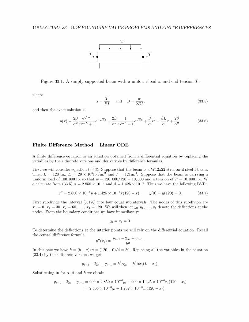
118LECTURE 33. ODE BOUNDARYVALUE PROBLEMS AND FINITE DIFFERENCES

t t -T T

? ? ? ? ?

w

Figure 33.1: A simply supported beam with a uniform load w and end tension T .

where

α =T

EIand β =

w

2EI, (33.5)

and then the exact solution is

y(x) =2β

α2

e√αL

e√αL + 1

e−√αx +

2β

α2

1

e√αL + 1

e√αx +

β

αx2 − βL

αx+

2β

α2. (33.6)

Finite Difference Method – Linear ODE

A finite difference equation is an equation obtained from a differential equation by replacing thevariables by their discrete versions and derivatives by difference formulas.

First we will consider equation (33.3). Suppose that the beam is a W12x22 structural steel I-beam.Then L = 120 in., E = 29 × 106lb./in.2 and I = 121in.4. Suppose that the beam is carrying auniform load of 100, 000 lb. so that w = 120, 000/120 = 10, 000 and a tension of T = 10, 000 lb.. We calculate from (33.5) α = 2.850× 10−6 and β = 1.425× 10−6. Thus we have the following BVP:

y′′ = 2.850× 10−6y + 1.425× 10−6x(120− x), y(0) = y(120) = 0. (33.7)

First subdivide the interval [0, 120] into four equal subintervals. The nodes of this subdivion arex0 = 0, x1 = 30, x2 = 60, . . . , x4 = 120. We will then let y0, y1, . . . , y4 denote the deflections at thenodes. From the boundary conditions we have immediately:

y0 = y4 = 0.

To determine the deflections at the interior points we will rely on the differential equation. Recallthe central difference formula

y′′(xi) ≈yi+1 − 2yi + yi−1

h2.

In this case we have h = (b− a)/n = (120− 0)/4 = 30. Replacing all the variables in the equation(33.4) by their discrete versions we get

yi+1 − 2yi + yi−1 = h2αyi + h2βxi(L− xi).

Substituting in for α, β and h we obtain:

yi+1 − 2yi + yi−1 = 900× 2.850× 10−6yi + 900× 1.425× 10−6xi(120− xi)

= 2.565× 10−3yi + 1.282× 10−3xi(120− xi).

119

This equation makes sense for i = 1, 2, 3. At x1 = 30, the equation becomes:

y2 − 2y1 + y0 = 2.565× 10−3y1 + 1.282× 10−3 × 30(90)

⇔ y2 − 2.002565y1 = 3.463.(33.8)

Note that this equation is linear in the unknowns y1 and y2. At x2 = 60 we have:

y3 − 2y2 + y1 = .002565y2 + 1.282× 10−3 × 602

⇔ y3 − 2.002565y2 + y1 = 4.615.(33.9)

At x3 = 90 we have (since y4 = 0)

−2.002565y3 + y2 = 3.463. (33.10)

Thus (y1, y2, y3) is the solution of the linear system:

−2.002565 1 0 3.4631 −2.002565 1 4.6150 1 −2.002565 3.463

.

We can easily find the solution of this system in Matlab:> A = [ -2.002565 1 0 ; 1 -2.002565 1 ; 0 1 -2.002565]

> b = [ 3.463 4.615 3.463 ]’

> y = A\b

To graph the solution, we need define the x values and add on the values at the endpoints:> x = 0:30:120

> y = [0 ; y ; 0]

> plot(x,y,’d’)

Adding a spline will result in an excellent graph.

The exact solution of this BVP is given in (33.6). That equation, with the parameter values for theW12x22 I-beam as in the example, is in the program myexactbeam.m on the web site. We can plotthe true solution on the same graph:> hold on

> myexactbeam

Thus our numerical solution is extremely good considering how few subintervals we used and howvery large the deflection is.

An amusing exercise is to set T = 0 in the program myexactbeam.m; the program fails because theexact solution is no longer valid. Also try T = .1 for which you will observe loss of precision. Onthe other hand the finite difference method still works when we set T = 0.

Exercises

33.1 Derive the finite difference equations for the BVP (33.7) on the same domain ([0, 120]), butwith eight subintervals and solve (usingMatlab) as in the example. Plot your result, togetheron the same plot with the exact solution (33.6) from the program myexactbeam.m.

33.2 By replacing y′′ and y′ with central differences, derive the finite difference equation for theBVP:

y′′ + y′ − y = x with y(0) = y(1) = 0

with 4 subintervals. Solve them and plot the solution using Matlab.

Lecture 34

Finite Difference Method – NonlinearODE

Heat conduction with radiation

If we again consider the heat in a metal bar of length L, but this time consider the effect of radiationas well as conduction, then the steady state equation has the form

uxx − d(u4 − u4b) = −g(x), (34.1)

where ub is the temperature of the background, d incorporates a coefficient of radiation and g(x) isthe heat source.

If we again replace the continuous problem by its discrete approximation then we get

ui+1 − 2ui + ui−1

h2− d(u4

i − u4b) = −gi = −g(xi). (34.2)

This equation is nonlinear in the unknowns, thus we no longer have a system of linear equationsto solve, but a system of nonlinear equations. One way to solve these equations would be by themultivariable Newton method. Instead, we introduce another interative method.

Relaxation Method for Nonlinear Finite Differences

We can rewrite equation (34.2) as

ui+1 − 2ui + ui−1 = h2d(u4i − u4

b)− h2gi.

From this we can solve for ui in terms of the other quantities:

2ui = ui+1 + ui−1 − h2d(u4i − u4

b) + h2gi.

Next we add ui to both sides of the equation to obtain

3ui = ui+1 + ui + ui−1 − h2d(u4i − u4

b) + h2gi,

and then divide by 3 to get

ui =1

3(ui+1 + ui + ui−1)−

h2

3

(

d(u4i − u4

b) + gi)

.

Now for the main idea. We will begin with an initial guess for the value of ui for each i, which wecan represent as a vector u0. Then we will use the above equation to get better estimates, u1, u2,. . . , and hope that they converge to the correct answer.

120

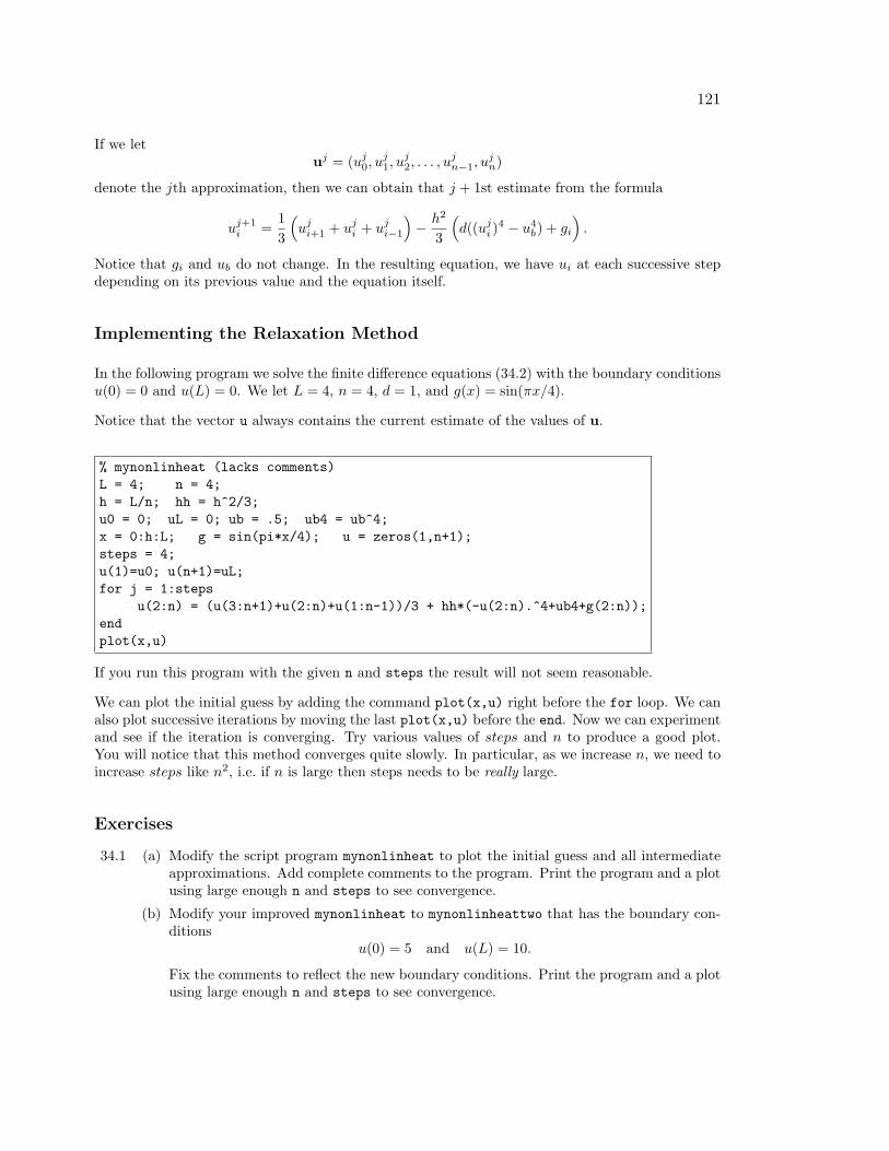
121

If we letuj = (uj

0, uj1, u

j2, . . . , u

jn−1, u

jn)

denote the jth approximation, then we can obtain that j + 1st estimate from the formula

uj+1i =

1

3

(

uji+1 + uj

i + uji−1

)

− h2

3

(

d((uji )

4 − u4b) + gi

)

.

Notice that gi and ub do not change. In the resulting equation, we have ui at each successive stepdepending on its previous value and the equation itself.

Implementing the Relaxation Method

In the following program we solve the finite difference equations (34.2) with the boundary conditionsu(0) = 0 and u(L) = 0. We let L = 4, n = 4, d = 1, and g(x) = sin(πx/4).

Notice that the vector u always contains the current estimate of the values of u.

% mynonlinheat (lacks comments)

L = 4; n = 4;

h = L/n; hh = h^2/3;

u0 = 0; uL = 0; ub = .5; ub4 = ub^4;

x = 0:h:L; g = sin(pi*x/4); u = zeros(1,n+1);

steps = 4;

u(1)=u0; u(n+1)=uL;

for j = 1:steps

u(2:n) = (u(3:n+1)+u(2:n)+u(1:n-1))/3 + hh*(-u(2:n).^4+ub4+g(2:n));

end

plot(x,u)

If you run this program with the given n and steps the result will not seem reasonable.

We can plot the initial guess by adding the command plot(x,u) right before the for loop. We canalso plot successive iterations by moving the last plot(x,u) before the end. Now we can experimentand see if the iteration is converging. Try various values of steps and n to produce a good plot.You will notice that this method converges quite slowly. In particular, as we increase n, we need toincrease steps like n2, i.e. if n is large then steps needs to be really large.

Exercises

34.1 (a) Modify the script program mynonlinheat to plot the initial guess and all intermediateapproximations. Add complete comments to the program. Print the program and a plotusing large enough n and steps to see convergence.

(b) Modify your improved mynonlinheat to mynonlinheattwo that has the boundary con-ditions

u(0) = 5 and u(L) = 10.

Fix the comments to reflect the new boundary conditions. Print the program and a plotusing large enough n and steps to see convergence.

Lecture 35

Parabolic PDEs - Explicit Method

Heat Flow and Diffusion

In the previous sections we studied PDE that represent steady-state heat problem. There was notime variable in the equation. In this section we begin to study how to solve equations that involvetime, i.e. we calculate temperature profiles that are changing.

The conduction of heat and diffusion of a chemical happen to be modeled by the same differentialequation. The reason for this is that they both involve similar processes. Heat conduction occurswhen hot, fast moving molecules bump into slower molecules and transfer some of their energy. In asolid this involves moles of molecules all moving in different, nearly random ways, but the net effectis that the energy eventually spreads itself out over a larger region. The diffusion of a chemical in agas or liquid simliarly involves large numbers of molecules moving in different, nearly random ways.These molecules eventually spread out over a larger region.

In three dimensions, the equation that governs both of these processes is the heat/diffusion equation

ut = c∆u ,

where c is the coefficient of conduction or diffusion, and ∆u(x, y, z) = uxx+uyy+uzz. The symbol ∆in this context is called the Laplacian. If there is also a heat/chemical source, then it is incorporateda function g(x, y, z, t) in the equation as

ut = c∆u+ g.

In some problems the z dimension is irrelevent, either because the object in question is very thin,or u does not change in the z direction. In this case the equation is

ut = c∆u = c(uxx + uyy).

Finally, in some cases only the x direction matters. In this case the equation is just

ut = cuxx, (35.1)

orut = cuxx + g(x, t). (35.2)

In this lecture we will learn a straight-forward technique for solving (35.1) and (35.2). It is verysimilar to the finite difference method we used for nonlinear boundary value problems.

It is worth mentioning a related equation

ut = c∆(uγ) for γ > 1 ,

122

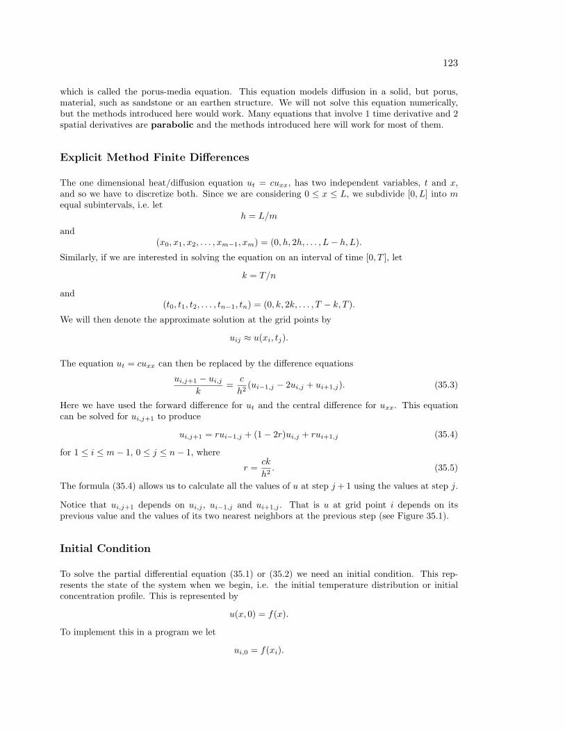
123

which is called the porus-media equation. This equation models diffusion in a solid, but porus,material, such as sandstone or an earthen structure. We will not solve this equation numerically,but the methods introduced here would work. Many equations that involve 1 time derivative and 2spatial derivatives are parabolic and the methods introduced here will work for most of them.

Explicit Method Finite Differences

The one dimensional heat/diffusion equation ut = cuxx, has two independent variables, t and x,and so we have to discretize both. Since we are considering 0 ≤ x ≤ L, we subdivide [0, L] into mequal subintervals, i.e. let

h = L/m

and(x0, x1, x2, . . . , xm−1, xm) = (0, h, 2h, . . . , L− h, L).

Similarly, if we are interested in solving the equation on an interval of time [0, T ], let

k = T/n

and(t0, t1, t2, . . . , tn−1, tn) = (0, k, 2k, . . . , T − k, T ).

We will then denote the approximate solution at the grid points by

uij ≈ u(xi, tj).

The equation ut = cuxx can then be replaced by the difference equations

ui,j+1 − ui,j

k=

c

h2(ui−1,j − 2ui,j + ui+1,j). (35.3)

Here we have used the forward difference for ut and the central difference for uxx. This equationcan be solved for ui,j+1 to produce

ui,j+1 = rui−1,j + (1− 2r)ui,j + rui+1,j (35.4)

for 1 ≤ i ≤ m− 1, 0 ≤ j ≤ n− 1, where

r =ck

h2. (35.5)

The formula (35.4) allows us to calculate all the values of u at step j +1 using the values at step j.

Notice that ui,j+1 depends on ui,j , ui−1,j and ui+1,j . That is u at grid point i depends on itsprevious value and the values of its two nearest neighbors at the previous step (see Figure 35.1).

Initial Condition

To solve the partial differential equation (35.1) or (35.2) we need an initial condition. This rep-resents the state of the system when we begin, i.e. the initial temperature distribution or initialconcentration profile. This is represented by

u(x, 0) = f(x).

To implement this in a program we let

ui,0 = f(xi).

124 LECTURE 35. PARABOLIC PDES - EXPLICIT METHOD

x x x x x

x | | | x

x x ui,j+1x x

x x x x x

6

tj

tj+1

xi−1 xi xi+1

Figure 35.1: The value at grid point i depends on its previous values and the previousvalues of its nearest neighbors.

Boundary Conditions

To solve the partial differential equation (35.1) or (35.2) we also need boundary conditions. Justas in the previous section we will have to specify something about the ends of the domain, i.e. atx = 0 and x = L. One possibility is fixed boundary conditions, which we can implement just as wedid for the ODE boundary value problem.

A second possibility is called variable boundary conditions. This is represented by time-dependent functions,

u(0, t) = g1(t) and u(L, t) = g2(t).

In a heat problem, g1 and g2 would represent heating or cooling applied to the ends. These areeasily implemented in a program by letting u0,j = g1(tj) and um,j = g2(tj).

Implementation

The following program (also available on the web page) implements the explicit method. It in-corporates variable boundary conditions at both ends. To run it you must define functions f , g1and g2. Notice that the main loop has only one line. The values of u are kept as a matrix. It isoften convenient to define a matrix of the right dimension containing all zeros, and then fill in thecalculated values as the program runs.

Run this program using L = 2, T = 20, f(x) = .5x, g1(t) = 0, and g2(t) = cos(t). Note that g1(t)must be input as g1 = inline(’0*t’).

125

function [t x u] = myheat(f,g1,g2,L,T,m,n,c)

% function [t x u] = myheat(f,g1,g2,L,T,m,n,c)

% solve u_t = c u_xx for 0<=x<=L, 0<=t<=T

% BC: u(0, t) = g1(t); u(L,t) = g2(t)

% IC: u(x, 0) = f(x)

% Inputs:

% f -- inline function for IC

% g1,g2 -- inline functions for BC

% L -- length of rod

% T -- length of time interval

% m -- number of subintervals for x

% n -- number of subintervals for t

% c -- rate constant in equation

% Outputs:

% t -- vector of time points

% x -- vector of x points

% u -- matrix of the solution, u(i,j)~=u(x(i),t(j))

h = L/m; k = T/n;

r = c*k/h^2; rr = 1 - 2*r;

x = linspace(0,L,m+1);

t = linspace(0,T,n+1);

%Set up the matrix for u:

u = zeros(m+1,n+1);

% assign initial conditions

u(:,1) = f(x);

% assign boundary conditions

u(1,:) = g1(t); u(m+1,:) = g2(t);

% find solution at remaining time steps

for j = 1:n

u(2:m,j+1) = r*u(1:m-1,j) + rr*u(2:m,j) + r*u(3:m+1,j);

end

% plot the results

mesh(x,t,u’)

Exercises

35.1 Run the program myheat.m with L = 2π, T = 20, c = .5, g1(t) = sin(t), g2(t) = 0 andf(x) = − sin(x/4). Set m = 20 and experiment with n. Get a plot when the program isstable and one when it isn’t. Turn in the plots.

35.2 Make a version of the program myheat.m so that k is an input instead of n and so that it stopswhen the maximum temperature in the bar is less than an input tempthres. For L = 2π,c = .01, g1(t) = 0, g2(t) = 10, f(x) = 100 and m = 10, set k so that the method will bestable. When is the temperature in the bar less than 20?

Lecture 36

Solution Instability for the ExplicitMethod

As we saw in experiments using myheat.m, the solution can become unbounded unless the timesteps are small. In this lecture we consider why.

Writing the Difference Equations in Matrix Form

If we use the boundary conditions u(0) = u(L) = 0 then the explicit method of the previous sectionhas the form:

ui,j+1 = rui−1,j + (1− 2r)ui,j + rui+1,j , 1 ≤ i ≤ m− 1, 0 ≤ j ≤ n− 1, (36.1)

where u0,j = 0 and um,j = 0. This is equivalent to the matrix equation

uj+1 = Auj , (36.2)

where uj is the column vector (u1,j , u2,j , . . . , um,j)′ representing the state at the jth time step and

A is the matrix

A =

1− 2r r 0 · · · 0

r 1− 2r r. . .

...

0. . .

. . .. . . 0

.... . . r 1− 2r r

0 · · · 0 r 1− 2r

. (36.3)

Unfortunately, this matrix can have a property which is very bad in this context. Namely, it cancause exponential growth of error unless r is small. To see how this happens, suppose that Uj isthe vector of correct values of u at time step tj and Ej is the error of the approximation uj , then

uj = Uj +Ej .

From (36.2), the approximation at the next time step will be

uj+1 = AUj +AEj ,

and if we continue for k steps,uj+k = AkUj +AkEj .

The problem with this is the term AkEj . This term is exactly what we would do in the powermethod for finding the eigenvalue of A with the largest absolute value. If the matrix A has ew’swith absolute value greater than 1, then this term will grow exponentially. Figure 36.1 shows thelargest absolute value of an ew of A as a function of the parameter r for various sizes of the matrixA. As you can see, for r > 1/2 the largest absolute ew grows rapidly for any m and quickly becomesgreater than 1.

126

127

0 0.1 0.2 0.3 0.4 0.5 0.6 0.7 0.8 0.9 10

0.5

1

1.5

2

2.5

3

r

EW m=2

m=3

Figure 36.1: Maximum absolute eigenvalue EW as a function of r for the matrix A fromthe explicit method for the heat equation calculated for matrices A of sizes m = 2 . . . 10.Whenever EW > 1 the method is unstable, i.e. errors grow exponentially with each step.When using the explicit method r < 1/2 is a safe choice.

Consequences

Recall that r = ck/h2. Since this must be less than 1/2, we have

k <h2

2c.

The first consequence is obvious: k must be relatively small. The second is that h cannot be toosmall. Since h2 appears in the formula, making h small would force k to be extremely small!

A third consequence is that we have a converse of this analysis. Suppose r < .5. Then all theeigenvalues will be less than one. Recall that the error terms satisfy

uj+k = AkUj +AkEj .

If all the eigenvalues of A are less than 1 in absolute value then AkEj grows smaller and smaller ask increases. This is really good. Rather than building up, the effect of any error diminishes as timepasses! From this we arrive at the following principle: If the explicit numerical solution for aparabolic equation does not blow up, then errors from previous steps fade away!

Finally, we note that if we have other boundary conditions then instead of equation (36.2) we have

uj+1 = Auj + rbj , (36.4)

where the first and last entries of bj contain the boundary conditions and all the other entries arezero. In this case the errors behave just as before, if r > 1/2 then the errors grow and if r < 1/2the errors fade away.

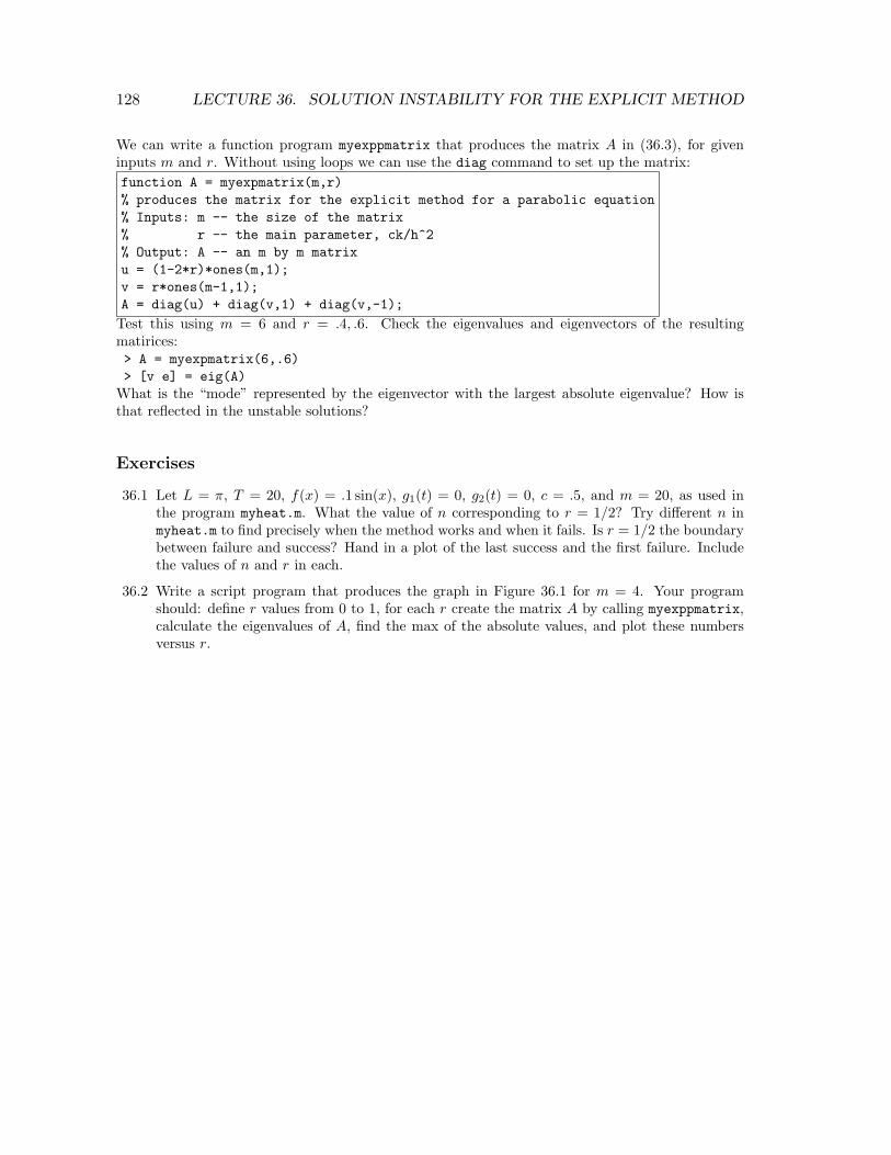
128 LECTURE 36. SOLUTION INSTABILITY FOR THE EXPLICIT METHOD

We can write a function program myexppmatrix that produces the matrix A in (36.3), for giveninputs m and r. Without using loops we can use the diag command to set up the matrix:

function A = myexpmatrix(m,r)

% produces the matrix for the explicit method for a parabolic equation

% Inputs: m -- the size of the matrix

% r -- the main parameter, ck/h^2

% Output: A -- an m by m matrix

u = (1-2*r)*ones(m,1);

v = r*ones(m-1,1);

A = diag(u) + diag(v,1) + diag(v,-1);

Test this using m = 6 and r = .4, .6. Check the eigenvalues and eigenvectors of the resultingmatirices:> A = myexpmatrix(6,.6)

> [v e] = eig(A)

What is the “mode” represented by the eigenvector with the largest absolute eigenvalue? How isthat reflected in the unstable solutions?

Exercises

36.1 Let L = π, T = 20, f(x) = .1 sin(x), g1(t) = 0, g2(t) = 0, c = .5, and m = 20, as used inthe program myheat.m. What the value of n corresponding to r = 1/2? Try different n inmyheat.m to find precisely when the method works and when it fails. Is r = 1/2 the boundarybetween failure and success? Hand in a plot of the last success and the first failure. Includethe values of n and r in each.

36.2 Write a script program that produces the graph in Figure 36.1 for m = 4. Your programshould: define r values from 0 to 1, for each r create the matrix A by calling myexppmatrix,calculate the eigenvalues of A, find the max of the absolute values, and plot these numbersversus r.

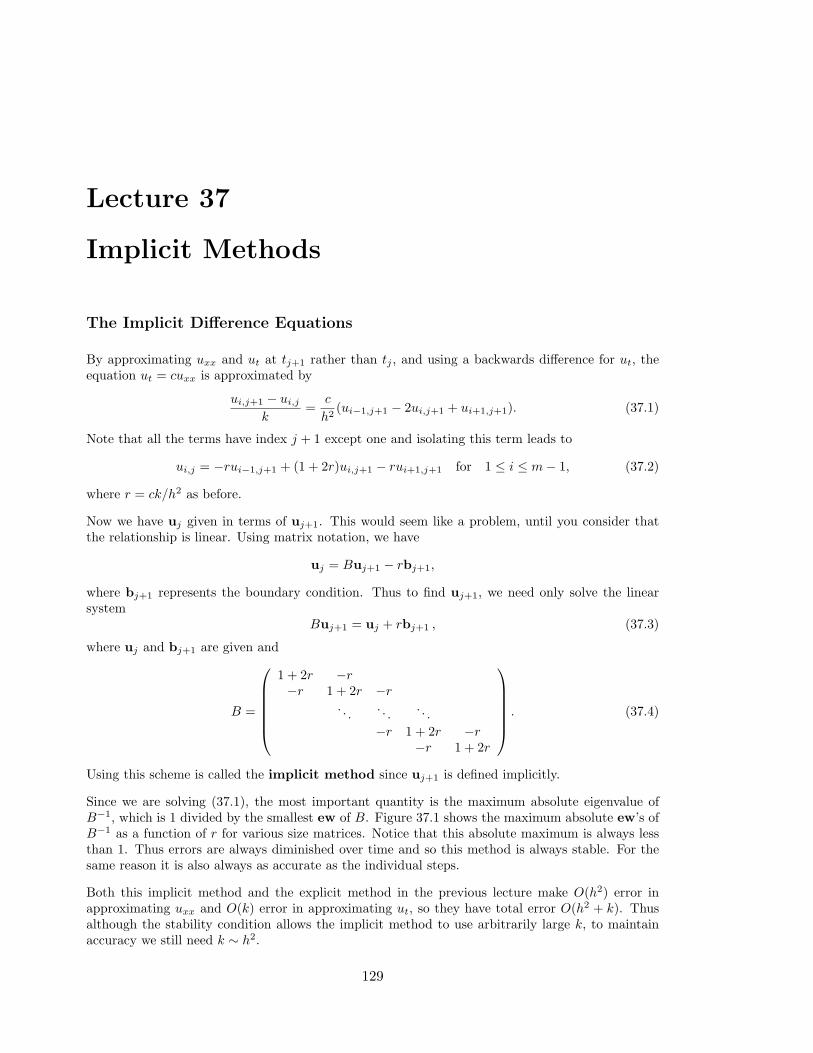
Lecture 37

Implicit Methods

The Implicit Difference Equations

By approximating uxx and ut at tj+1 rather than tj , and using a backwards difference for ut, theequation ut = cuxx is approximated by

ui,j+1 − ui,j

k=

c

h2(ui−1,j+1 − 2ui,j+1 + ui+1,j+1). (37.1)

Note that all the terms have index j + 1 except one and isolating this term leads to

ui,j = −rui−1,j+1 + (1 + 2r)ui,j+1 − rui+1,j+1 for 1 ≤ i ≤ m− 1, (37.2)

where r = ck/h2 as before.

Now we have uj given in terms of uj+1. This would seem like a problem, until you consider thatthe relationship is linear. Using matrix notation, we have

uj = Buj+1 − rbj+1,

where bj+1 represents the boundary condition. Thus to find uj+1, we need only solve the linearsystem

Buj+1 = uj + rbj+1 , (37.3)

where uj and bj+1 are given and

B =

1 + 2r −r−r 1 + 2r −r

. . .. . .

. . .

−r 1 + 2r −r−r 1 + 2r

. (37.4)

Using this scheme is called the implicit method since uj+1 is defined implicitly.

Since we are solving (37.1), the most important quantity is the maximum absolute eigenvalue ofB−1, which is 1 divided by the smallest ew of B. Figure 37.1 shows the maximum absolute ew’s ofB−1 as a function of r for various size matrices. Notice that this absolute maximum is always lessthan 1. Thus errors are always diminished over time and so this method is always stable. For thesame reason it is also always as accurate as the individual steps.

Both this implicit method and the explicit method in the previous lecture make O(h2) error inapproximating uxx and O(k) error in approximating ut, so they have total error O(h2 + k). Thusalthough the stability condition allows the implicit method to use arbitrarily large k, to maintainaccuracy we still need k ∼ h2.

129

130 LECTURE 37. IMPLICIT METHODS

0 0.2 0.4 0.6 0.8 1 1.2 1.4 1.6 1.8 2

0.4

0.5

0.6

0.7

0.8

0.9

1

r

EW

m = 2m = 3

Figure 37.1: Maximum absolute eigenvalue EW as a function of r for the matrix B−1 fromthe implicit method for the heat equation calculated for matrices B of sizes m = 2 . . . 10.Whenever EW < 1 the method is stable, i.e. it is always stable.

Crank-Nicholson Method

Now that we have two different methods for solving parabolic equation, it is natural to ask, “canwe improve by taking an average of the two methods?” The answer is yes.

We implement a weighted average of the two methods by considering an average of the approxima-tions of uxx at j and j + 1. This leads to the equations

ui,j+1 − ui,j

k=

λc

h2(ui−1,j+1 − 2ui,j+1 + ui+1,j+1) +

(1− λ)c

h2(ui−1,j − 2ui,j + ui+1,j). (37.5)

The implicit method contained in these equations is called the Crank-Nicholson method. Gath-ering terms yields the equations

−rλui−1,j+1 + (1 + 2rλ)ui,j+1 − rλui+1,j+1 = r(1− λ)ui−1,j + (1− 2r(1− λ))ui,j + r(1− λ)ui+1,j .

In matrix notation this is

Bλuj+1 = Aλuj + rbj+1,

where

Aλ =

1− 2(1− λ)r (1− λ)r(1− λ)r 1− 2(1− λ)r (1− λ)r

. . .. . .

. . .

(1− λ)r 1− 2(1− λ)r (1− λ)r(1− λ)r 1− 2(1− λ)r

(37.6)

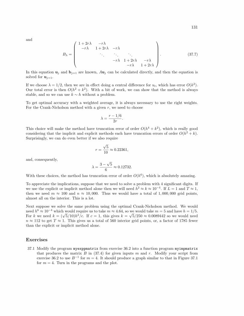
131

and

Bλ =

1 + 2rλ −rλ−rλ 1 + 2rλ −rλ

. . .. . .

. . .

−rλ 1 + 2rλ −rλ−rλ 1 + 2rλ

. (37.7)

In this equation uj and bj+1 are known, Auj can be calculated directly, and then the equation issolved for uj+1.

If we choose λ = 1/2, then we are in effect doing a central difference for ut, which has error O(k2).Our total error is then O(h2 + k2). With a bit of work, we can show that the method is alwaysstable, and so we can use k ∼ h without a problem.

To get optimal accuracy with a weighted average, it is always necessary to use the right weights.For the Crank-Nicholson method with a given r, we need to choose

λ =r − 1/6

2r.

This choice will make the method have truncation error of order O(h4 + k2), which is really goodconsidering that the implicit and explicit methods each have truncation errors of order O(h2 + k).Surprisingly, we can do even better if we also require

r =

√5

10≈ 0.22361,

and, consequently,

λ =3−

√5

6≈ 0.12732.

With these choices, the method has truncation error of order O(h6), which is absolutely amazing.

To appreciate the implications, suppose that we need to solve a problem with 4 significant digits. Ifwe use the explicit or implicit method alone then we will need h2 ≈ k ≈ 10−4. If L = 1 and T ≈ 1,then we need m ≈ 100 and n ≈ 10, 000. Thus we would have a total of 1, 000, 000 grid points,almost all on the interior. This is a lot.

Next suppose we solve the same problem using the optimal Crank-Nicholson method. We wouldneed h6 ≈ 10−4 which would require us to take m ≈ 4.64, so we would take m = 5 and have h = 1/5.For k we need k = (

√5/10)h2/c. If c = 1, this gives k =

√5/250 ≈ 0.0089442 so we would need

n ≈ 112 to get T ≈ 1. This gives us a total of 560 interior grid points, or, a factor of 1785 fewerthan the explicit or implicit method alone.

Exercises

37.1 Modify the program myexppmatrix from exercise 36.2 into a function program myimpmatrix

that produces the matrix B in (37.4) for given inputs m and r. Modify your script fromexercise 36.2 to use B−1 for m = 4. It should produce a graph similar to that in Figure 37.1for m = 4. Turn in the programs and the plot.

Lecture 38

Insulated Boundary Conditions

Insulation

In many of the previous sections we have considered fixed boundary conditions, i.e. u(0) = a,u(L) = b. We implemented these simply by assigning uj

0 = a and ujn = b for all j.

We also considered variable boundary conditions, such as u(0, t) = g1(t). For example, we mighthave u(0, t) = sin(t) which could represents periodic heating and cooling of the end at x = 0.

A third important type of boundary condition is called the insulated boundary condition. It is sonamed because it mimics an insulator at the boundary. Physically, the effect of insulation is thatno heat flows across the boundary. This means that the temperature gradient is zero, which impliesthat should require the mathematical boundary condition u′(L) = 0.

To use it in a program, we must replace u′(L) = 0 by a discrete version. Recall that in our discreteequations we usually have L = xn. Recall from the section on numerical derivatives, that there arethree different ways to replace a derivative by a difference equation, left, right and central differences.The three of them at xn would be:

u′(xn) ≈un − un−1

h≈ un+1 − un

h≈ un+1 − un−1

2h.

If xn is the last node of our grid, then it is clear that we cannot use the right or central difference,but are stuck with the first of these. Setting that expression to zero implies:

un = un−1.

This restriction can be easily implemented in a program simply by putting a statement u(n+1)=u(n)inside the loop that updates values of the profile. However, since this method replaces u′(L) = 0 byan expression that is only accurate to first order, it is not very accurate and is usually avoided.

Instead we want to use the most accurate version, the central difference. For that we should have

u′(L) = u′(xn) =un+1 − un−1

2h= 0.

or simplyun+1 = un−1.

However, un+1 would represent u(xn+1) and xn+1 would be L + h, which is outside the domain.This however is not an obstacle in a program. We can simply extend the grid to one more node,xn+1, and let un+1 always equal un−1 by copying un−1 into un+1 whenever un−1 changes. Thepoint xn+1 is “fictional”, but a computer does not know the difference between fiction and reality!This idea is carried out in the calculations of the next section and illustrated in Figure 38.1.

132

133

6u

u u u e

uu

ue-copy

xn−2 xn−1 xn xn+1

Figure 38.1: Illustation of an insulated boundary condition using a fictional point xn+1

with un+1 = un−1.

A way to think of an insulated boundary that makes sense of the point L+h is to think of two barsjoined end to end, where you let the second bar be mirror image of the first bar. If you do this,then no heat will flow across the joint, which is exactly the same effect as insulating.

Another practical way to implement an insulated boundary is to let the grid points straddle theboundary. For example suppose we want to impose insulated boundary at the left end of a bar, i.e.u′(0) = 0, then you could let the first two grid points be at x0 = −h/2 and x1 = h/2. Then youcan let

u0 = u1.

This will again force the central difference at x = 0 to be 0.

Implementation in a linear equation by elimination

Consider the BVP:uxx = −1, u(0) = 5, u′(1) = 0. (38.1)

This represents the steady state temperature of a bar with a uniformly applied heat source, withone end held at a fixed temperature and the other end insulated.

If we use 4 equally spaced intervals, then

m = 4, L = 1, ⇒ h =L

m=

1

4,

andx0 = 0, x1 = .25, x2 = .5, x3 = .75, x4 = 1, and x5 = 1.25.

The point x5 = 1.25 is outside the region and thus fictional. The boundary condition at x0 = 0 isimplemented as

u0 = 5.

For the insulated condition, we will require:

u5 = u3.

This makes the central difference for u′(x4) be zero. We can write the differential equation as adifference equation:

ui−1 − 2ui + ui+1

h2= −1

orui−1 − 2ui + ui+1 = −0.0625, i = 1, 2, 3, 4.

134 LECTURE 38. INSULATED BOUNDARY CONDITIONS

For i = 1, recalling that u0 = 5 we have:

5− 2u1 + u2 = −.0625 or − 2u1 + u2 = −5.0625.

For i = 2 and i = 3 we have:

u1 − 2u2 + u3 = −.0625 and u2 − 2u3 + u4 = −.0625.

For i = 4 we have:u3 − 2u4 + u5 = −.5.

Note that we now have 5 unknowns in our problem: u1, . . . , u5. However, from the boundarycondition u5 = u3 and so we can eliminate u5 from our equations and write:

2u3 − 2u4 = −.0625.

Summarizing, we can put the unknown quantities in a vector u = (u1, u2, u3, u4)′ and write the

equations as a matrix equation Au = b where:

A=

−2 1 0 01 −2 1 00 1 −2 10 0 2 −2

and b = (−5.0625,−.0625,−.0625.− .0625)′. Solve this system and plot the results:> u = A\b

> u = [5 ; u]

> x = 0:.25:1

> plot(x,u,’d’)

the interpolate with a spline.

The exact solution of this BVP is:U(x) = 5 + x− .5x2.

Use hold on and plot this function on the same graph to compare. > xx = 0:.01:1; > uu = 5 + xx - .5*xx.^2;

should see that our approximate solution almost perfect!

Insulated boundary conditions in time-dependent problems

To implement the insulated boundary condition in an explicit difference equation with time, weneed to copy values from inside the region to fictional points just outside the region. See Figure 38.2for an illustration.

An example

The steady state temperature u(r) (given in polar coordinates) of a disk subjected to a radiallysymmetric heat load g(r) and cooled by conduction to the rim of the disk and radiation to itsenvironment is determined by the boundary value problem:

∂2u

∂r2+

1

r

∂u

∂r= d(u4 − u4

b)− g(r) with u(R) = uR and u′(0) = 0. (38.2)

Here ub is the (fixed) background temperature and uR is the (fixed) temperature at the rim of thedisk.

135

x x x x h

x x x x h

x x x x h

x x x x h

6 6 6

6 6 6

6 6 6

@@

@I

@@

@I

@@

@I

@@

@I

@@

@I

@@

@I

@@

@I

@@

@I

@@

@I

R

R

R

R

tj

tj+1

xm−1 xm xm+1

Figure 38.2: Illustration of information flow for the explicit method with an insulatedboundary condition. The open circles are the fictional points and the curved arrows repre-sent copying the value.

The class web site has a program myheatdisk.m that implements these equations for parametervalues R = 5, d = .1, uR = ub = 10 and g(r) = (r − 5)2. Notice that the equations have asingularity (discontinuity) at r = 0. How does the program avoid this problem? How does theprogram implement uR = 10 and u′(0) = 0? Run the program.

Exercises

38.1 Redo the calculations for the BVP (38.1) except do not include the fictional point x5. Instead,let x4 be the last point and impose the insulated boundary by requiring u4 = u3. (Your systemof equations should be 3 × 3.) Compare this solution with the true solution and the betterapproximation in the lecture. Illustrate this comparison on a single plot.

38.2 Modify the program myheat.m to have an insulated boundary at x = L (rather than u(L, t) =g2(t)). You will need to change the domain to: x = 0:h:L+h and change the dimensions ofall the other objects to fit this domain. Run the program with L = 2π, T = 20, c = .5,g1(t) = sin(t) and f(x) = − sin(x/4). Set m = 20 and experiment with n. Get a plot whenthe program is stable. Turn in your program and plots.

Lecture 39

Finite Difference Method for EllipticPDEs

Examples of Elliptic PDEs

Elliptic PDE’s are equations with second derivatives in space and no time derivative. The mostimportant examples are Laplace’s equation

∆u = uxx + uyy + uzz = 0

and the Poisson equation

∆u = f(x, y, z).

These equations are used in a large variety of physical situations such as: steady state heat problems,steady state chemical distributions, electrostatic potentials, elastic deformation and steady statefluid flows.

For the sake of clarity we will only consider the two dimensional problem. A good model problemin this dimension is the elastic deflection of a membrane. Suppose that a membrane such as a sheetof rubber is stretched across a rectangular frame. If some of the edges of the frame are bent, or ifforces are applied to the sheet then it will deflect by an amount u(x, y) at each point (x, y). This uwill satify the boundary value problem:

uxx + uyy = f(x, y) for (x, y) in R,

u(x, y) = g(x, y) for (x, y) on ∂R,(39.1)

where R is the rectangle, ∂R is the edge of the rectangle, f(x, y) is the force density (pressure)applied at each point and g(x, y) is the deflection at the edge.

The Finite Difference Equations

Suppose the rectangle is described by

R = a ≤ x ≤ b, c ≤ y ≤ d.

We will divide R in subrectangles. If we have m subdivisions in the x direction and n subdivisionsin the y direction, then the step size in the x and y directions respectively are

h =b− a

mand k =

d− c

n.

136

137

We obtain the finite difference equations for (39.1) by replacing uxx and uyy by their central differ-ences to obtain

ui+1,j − 2uij + ui−1,j

h2+

ui,j+1 − 2uij + ui,j−1

k2= f(xi, yj) = fij (39.2)

for 1 ≤ i ≤ m− 1 and 1 ≤ j ≤ n− 1. The boundary conditions are introduced by:

u0,j = g(a, yj), um,j = g(b, yj), ui,0 = g(xi, c), and ui,n = g(xi, d). (39.3)

Direct Solution of the Equations

Notice that since the edge values are prescribed, there are (m − 1) × (n − 1) grid points where weneed to determine the solution. Note also that there are exactly (m − 1) × (n − 1) equations in(39.2). Finally, notice that the equations are all linear. Thus we could solve the equations exactlyusing matrix methods. To do this we would first need to express the uij ’s as a vector, rather thena matrix. To do this there is a standard procedure: let u be the column vector we get by placingone column after another from the columns of (uij). Thus we would list u:,1 first then u:,2, etc..Next we would need to write the matrix A that contains the coefficients of the equations (39.2) andincorporate the boundary conditions in a vector b. Then we could solve an equation of the form

Au = b. (39.4)

Setting up and solving this equation is called the direct method.

An advantage of the direct method is that solving (39.4) can be done relatively quickly and accu-rately. The drawback of the direct method is that one must set up u, A and b, which is confusing.Further, the matrix A has dimensions (m− 1)(n− 1)× (m− 1)(n− 1), which can be rather large.Although A is large, many of its elements are zero. Such a matrix is called sparse and there arespecial methods intended for efficiently working with sparse matrices.

Iterative Solution

A usually prefered alternative to the direct method described above is to solve the finite differenceequations iteratively. To do this, first solve (39.2) for uij , which yields

uij =1

2(h2 + k2)

(

k2(ui+1,j + ui−1,j) + h2(ui,j+1 + ui,j−1)− h2k2fij)

. (39.5)

This method is another example of a relaxation method. Using this formula, along with (39.3),we can update uij from its neighbors, just as we did in the relaxation method for the nonlinearboundary value problem. If this method converges, then the result is an approximate solution.

The iterative solution is implemented in the program mypoisson.m on the class web site. Downloadand read it. You will notice that maxit is set to 0. Thus the program will not do any iteration, butwill plot the initial guess. The initial guess in this case consists of the proper boundary values atthe edges, and zero everywhere in the interior. To see the solution evolve, gradually increase maxit.

138 LECTURE 39. FINITE DIFFERENCE METHOD FOR ELLIPTIC PDES

Exercises

39.1 Modify the program mypoisson.m (from the class web page) in the following ways:

• Change x = b to be an insulated boundary, i.e. ux(b, y) = 0.

• Change the force f(x, y) to a negative constant −p.

Experiment with various values of p and maxit. Obtain plots for small and large p. Tellhow many iterations are needed for convergence in each. For large p plot also a couple ofintermediate steps.

Lecture 40

Convection-Diffusion Equations

Exercises

40.1

139

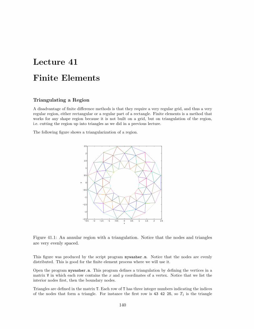
Lecture 41

Finite Elements

Triangulating a Region

A disadvantage of finite difference methods is that they require a very regular grid, and thus a veryregular region, either rectangular or a regular part of a rectangle. Finite elements is a method thatworks for any shape region because it is not built on a grid, but on triangulation of the region,i.e. cutting the region up into triangles as we did in a previous lecture.

The following figure shows a triangularization of a region.

−2.5 −2 −1.5 −1 −0.5 0 0.5 1 1.5 2 2.5−2.5

−2

−1.5

−1

−0.5

0

0.5

1

1.5

2

2.5

x

y

Figure 41.1: An annular region with a triangulation. Notice that the nodes and trianglesare very evenly spaced.

This figure was produced by the script program mywasher.m. Notice that the nodes are evenlydistributed. This is good for the finite element process where we will use it.

Open the program mywasher.m. This program defines a triangulation by defining the vertices in amatrix V in which each row contains the x and y coordinates of a vertex. Notice that we list theinterior nodes first, then the boundary nodes.

Triangles are defined in the matrix T. Each row of T has three integer numbers indicating the indicesof the nodes that form a triangle. For instance the first row is 43 42 25, so T1 is the triangle

140

141

t

DDDDDDDD

t

BBBBBBBB

t

AAAAAAAA

t

AAAAAAAA

t

BBBBBBBB

t

Figure 41.2: The finite elements for the triangulation of a one dimensional object.

with vertices v43, v42 and v25. The matrix T in this case was produced by the Matlab commanddelaunay. The command produced more triangles than desire and the unwanted ones were deleted.

We a three dimensional plot of the region and triangles is produced by having the last line betrimesh(T,x,y,z).

What is a finite element?

The finite element method is a mathematically complicated process. However, a finite element isactually a very simple object. To each node vj we associate a function Φj that has the propertiesΦj(vj) = 1 and Φj(vi) = 0 for i 6= j. Between nodes, Φj is a linear function. This function is thefinite element. (There are fancier types of finite elements that we will not discuss.)

If we consider one dimension, then a triangulation is just a subdivision into subintervals. In Fig-ure 41.2 we show an uneven subdivision of an interval and the finite elements corresponding to eachnode.

In two dimensions, Φj is composed of triangular piece of planes. Thus Φj is a function whose graphis a pyramid with its peak over node vj .

What is a finite element solution?

A finite element (approximate) solution is a linear combination of the elements:

U(x) =n∑

j=1

CjΦj(x). (41.1)

Thus finding a finite element solution amounts to finding the best values for the constants Cjnj=1.

In the program mywasher.m, the vector z contains the node values Cj . These values give the heightat each node in the graph. For instance if we set all equal to 0 except one equal to 1, then thefunction is a finite element. Do this for one boundary node, then for one interior node.

Notice that a sum of linear functions is a linear function. Thus the solution using linear elements isa piecewise linear function. Also notice that if we denote the j-th vertex by vj , then

U(vj) = Cj . (41.2)

Thus we see that the constants Cj are just the values at the nodes.

142 LECTURE 41. FINITE ELEMENTS

Take the one-dimensional case. Since we know that the solution is linear on each subinterval,knowing the values at the endpoints of the subintervals, i.e. the nodes, gives us complete knowledgeof the solution. Figure 41.3 could be a finite element solution since it is piecewise linear.

t

t

@@@

t

t t

AAAAAA

t

Figure 41.3: A possible finite element solution for a one dimensional object. Values areassigned at each node and a linear interpolant is used in between.

In the two-dimensional case, the solution is linear on each triangle, and so again, if we know thevalues Cjnj=1 at the nodes then we know everything.

Experiment with finite elements

By changing the values in c in the program we can produce different three dimensional shapes basedon the triangles. The point then of a finite element solution is to find the values at the nodes thatbest approximate the true solution. This task can be subdivided into two parts: (1) assigning thevalues at the boundary nodes and (2) assigning the values at the interior nodes.

Values at boundary nodes

Once a triangulation and a set of finite elements is set up, the next step is to incorporate theboundary conditions of the problem. Suppose that we have fixed boundary conditions, i.e. of theform

u(x) = g(x), for x ∈ ∂D,

where D is the object (domain) and ∂D is its boundary. Then the boundary condition directlydetermines the values on the boundary nodes.

In particular, suppose that vℓ is a boundary node. Since Φℓ(vℓ) = 1 and all the other elements arezero at node vℓ, then to make

U(vℓ) =n∑

j=1

CjΦj(vℓ) = g(vℓ),

we must choose

Cℓ = g(vℓ).

Thus the constants Cj for the boundary nodes are set at exactly the value of the bound-ary condition at the nodes.

143

Thus, if there are m interior nodes, then

Cj = g(vj), for all m+ 1 ≤ j ≤ n.

In the program mywasher the first 32 vertices correspond to interior nodes and the last 32 correspondto boundary nodes. By setting the last 32 values of z, we achieve the boundary conditions. Wecould do this by adding the following commands to the program:z(33:64) = .5;

or more elaborately we might use functions:z(33:48) = x(33:48).^2 - .5*y(33:48).^2;

z(49:64) = .2*cos(y(49:64));

Exercises

41.1 Generate an interesting or useful 2-d object and a well-distributed triangulation of it.

• Plot the region.

• Plot one interior finite element.

• Plot one boundary finite element.

• Assign values to the boundary using a function (or functions) and plot the region withthe boundary values.

Turn in your code and the four plots.

Lecture 42

Determining Internal Node Values

As seen in the previous section, a finite element solution of a boundary value problem boils down tofinding the best values of the constants Cjnj=1, which are the values of the solution at the nodes.The interior nodes values are determined by variational principles. Variational principles usuallyamount to minimizing internal energy. It is a physical principle that systems seek to be in astate of minimal energy and this principle is used to find the internal node values.

Variational Principles

For the differential equations that describe many physical systems, the internal energy of the systemis an integral. For instance, for the steady state heat equation

uxx + uyy = g(x, y) (42.1)

the internal energy is the integral

I[u] =

∫∫

R

u2x + u2

y + 2g(x, y)u(x, y) dA, (42.2)

where R is the region on which we are working. It can be shown that u(x, u) is a solution of (42.1)if and only if it is minimizer of I[u] in (42.2).

The finite element solution

Recall that a finite element solution is a linear combination of finite element functions:

U(x, y) =n∑

j=1

CjΦj(x, y),

where n is the number of nodes. To obtain the values at the internal nodes, we will plug U(x, y)into the energy integral and minimize. That is, we find the minimum of

I[U ]

for all choices of Cjmj=1, where m is the number of internal nodes. In this as with any otherminimization problem, the way to find a possible minimum is to differentiate the quantity withrespect to the variables and set the results to zero. In this case the free variables are Cjmj=1. Thusto find the minimizer we should try to solve

∂I[U ]

∂Cj= 0 for 1 ≤ j ≤ m. (42.3)

144

145

We call this set of equations the internal node equations. At this point we should ask whetherthe internal node equations can be solved, and if so, is the solution actually a minimizer (and nota maximizer). The following two facts answer these questions. These facts make the finite elementmethod practical:

• For most applications the internal node equations are linear.

• For most applications the internal node equations give a minimizer.

We can demonstrate the first fact using an example.

Application to the steady state heat equation

If we plug the candidate finite element solution U(x, y) into the energy integral for the heat equation(42.2), we obtain

I[U ] =

∫∫

R

Ux(x, y)2 + Uy(x, y)

2 + 2g(x, y)U(x, y) dA. (42.4)

Differentiating with respect to Cj we obtain the internal node equations

0 =

∫∫

R

2Ux∂Ux

∂Cj+ 2Uy

∂Uy

∂Cj+ 2g(x, y)

∂U

∂CjdA for 1 ≤ j ≤ m. (42.5)

Now we have several simplifications. First note that since

U(x, y) =

n∑

j=1

CjΦj(x, y),

we have∂U

∂Cj= Φj(x, y) .

Also note that

Ux(x, y) =

n∑

j=1

Cj∂

∂xΦj(x, y),

and so∂Ux

∂Cj= (Φj)x.

Similarly,∂Uy

∂Cj= (Φj)y. The integral (42.5) then becomes

0 = 2

∫∫

Ux(Φj)x + Uy(Φj)y + g(x, y)Φj(x, y) dA for 1 ≤ j ≤ m.

Next we use the fact that the region R is subdivided into triangles Tipi=1 and the functions inquestion have different definitions on each triangle. The integral then is a sum of the integrals:

0 = 2

p∑

i=1

∫∫

Ti

Ux(Φj)x + Uy(Φj)y + g(x, y)Φj(x, y) dA for 1 ≤ j ≤ m.

Now note that the function Φj(x, y) is linear on triangle Ti and so

Φij(x, y) = Φj |Ti(x, y) = aij + bijx+ cijy.

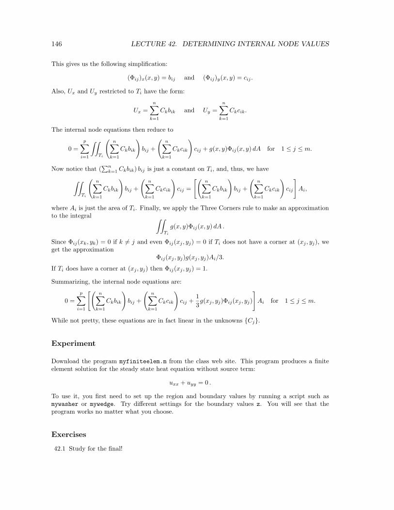
146 LECTURE 42. DETERMINING INTERNAL NODE VALUES

This gives us the following simplification:

(Φij)x(x, y) = bij and (Φij)y(x, y) = cij .

Also, Ux and Uy restricted to Ti have the form:

Ux =

n∑

k=1

Ckbik and Uy =

n∑

k=1

Ckcik.

The internal node equations then reduce to

0 =

p∑

i=1

∫∫

Ti

(

n∑

k=1

Ckbik

)

bij +

(

n∑

k=1

Ckcik

)

cij + g(x, y)Φij(x, y) dA for 1 ≤ j ≤ m.

Now notice that (∑n

k=1 Ckbik) bij is just a constant on Ti, and, thus, we have

∫∫

Ti

(

n∑

k=1

Ckbik

)

bij +

(

n∑

k=1

Ckcik

)

cij =

[(

n∑

k=1

Ckbik

)

bij +

(

n∑

k=1

Ckcik

)

cij

]

Ai,

where Ai is just the area of Ti. Finally, we apply the Three Corners rule to make an approximationto the integral

∫∫

Ti

g(x, y)Φij(x, y) dA .

Since Φij(xk, yk) = 0 if k 6= j and even Φij(xj , yj) = 0 if Ti does not have a corner at (xj , yj), weget the approximation

Φij(xj , yj)g(xj , yj)Ai/3.

If Ti does have a corner at (xj , yj) then Φij(xj , yj) = 1.

Summarizing, the internal node equations are:

0 =

p∑

i=1

[(

n∑

k=1

Ckbik

)

bij +

(

n∑

k=1

Ckcik

)

cij +1

3g(xj , yj)Φij(xj , yj)

]

Ai for 1 ≤ j ≤ m.

While not pretty, these equations are in fact linear in the unknowns Cj.

Experiment

Download the program myfiniteelem.m from the class web site. This program produces a finiteelement solution for the steady state heat equation without source term:

uxx + uyy = 0 .

To use it, you first need to set up the region and boundary values by running a script such asmywasher or mywedge. Try different settings for the boundary values z. You will see that theprogram works no matter what you choose.

Exercises

42.1 Study for the final!

Review of Part IV

Methods and Formulas

Initial Value Problems

Reduction to First order system:For an n-th order equation that can be solved for the n-th derivative:

x(n) = f

(

t, x, x, x, . . . ,dn−1x

dtn−1

)

. (42.6)

Then use the standard change of variables:

y1 = x

y2 = x

...

yn = x(n−1) =dn−1x

dtn−1.

(42.7)

Differentiating results in a first-order system:

y1 = x = y2

y2 = x = y3

...

yn = x(n) = f(t, y1, y2, . . . , yn).

(42.8)

Euler’s method:yi+1 = yi + hf(ti,yi).

Modified (or Improved) Euler method:

k1 = hf(ti,yi)

k2 = hf(ti + h,yi + k1)

yi+1 = yi +1

2(k1 + k2)

Boundary Value Probems

Finite Differences:Replace the Differential Equation by Difference Equations on a grid.Review the lecture on Numerical Differentiation.

147

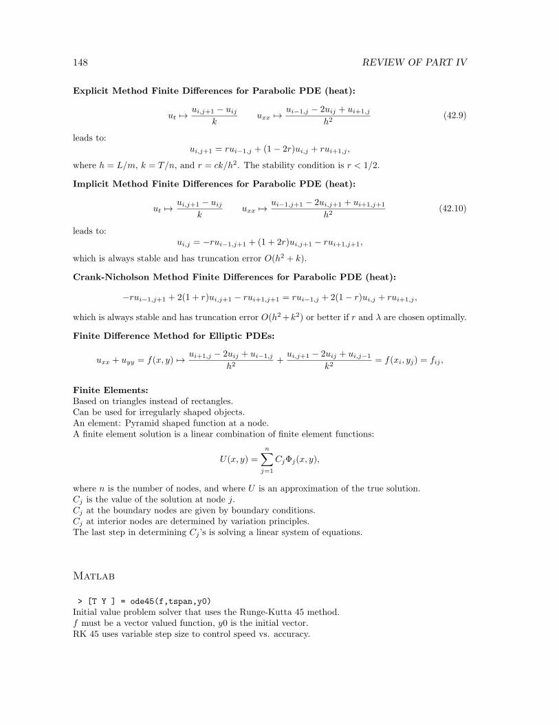
148 REVIEW OF PART IV

Explicit Method Finite Differences for Parabolic PDE (heat):

ut 7→ui,j+1 − uij

kuxx 7→ ui−1,j − 2uij + ui+1,j

h2(42.9)

leads to:ui,j+1 = rui−1,j + (1− 2r)ui,j + rui+1,j ,

where h = L/m, k = T/n, and r = ck/h2. The stability condition is r < 1/2.

Implicit Method Finite Differences for Parabolic PDE (heat):

ut 7→ui,j+1 − uij

kuxx 7→ ui−1,j+1 − 2ui,j+1 + ui+1,j+1

h2(42.10)

leads to:ui,j = −rui−1,j+1 + (1 + 2r)ui,j+1 − rui+1,j+1,

which is always stable and has truncation error O(h2 + k).

Crank-Nicholson Method Finite Differences for Parabolic PDE (heat):

−rui−1,j+1 + 2(1 + r)ui,j+1 − rui+1,j+1 = rui−1,j + 2(1− r)ui,j + rui+1,j ,

which is always stable and has truncation error O(h2+k2) or better if r and λ are chosen optimally.

Finite Difference Method for Elliptic PDEs:

uxx + uyy = f(x, y) 7→ ui+1,j − 2uij + ui−1,j

h2+

ui,j+1 − 2uij + ui,j−1

k2= f(xi, yj) = fij ,

Finite Elements:Based on triangles instead of rectangles.Can be used for irregularly shaped objects.An element: Pyramid shaped function at a node.A finite element solution is a linear combination of finite element functions:

U(x, y) =n∑

j=1

CjΦj(x, y),

where n is the number of nodes, and where U is an approximation of the true solution.Cj is the value of the solution at node j.Cj at the boundary nodes are given by boundary conditions.Cj at interior nodes are determined by variation principles.The last step in determining Cj ’s is solving a linear system of equations.

Matlab

> [T Y ] = ode45(f,tspan,y0)

Initial value problem solver that uses the Runge-Kutta 45 method.f must be a vector valued function, y0 is the initial vector.RK 45 uses variable step size to control speed vs. accuracy.

Part V

Appendices

c©Copyright, Todd Young and Martin Mohlenkamp, Mathematics Department, Ohio University, 2007

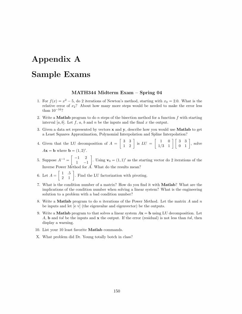
Appendix A

Sample Exams

MATH344 Midterm Exam – Spring 04

1. For f(x) = x2 − 5, do 2 iterations of Newton’s method, starting with x0 = 2.0. What is therelative error of x2? About how many more steps would be needed to make the error lessthan 10−16?

2. Write a Matlab program to do n steps of the bisection method for a function f with startinginterval [a, b]. Let f , a, b and n be the inputs and the final x the output.

3. Given a data set represented by vectors x and y, describe how you would use Matlab to geta Least Squares Approximation, Polynomial Interpolation and Spline Interpolation?

4. Given that the LU decomposition of A =

[

3 31 2

]

is LU =

[

1 01/3 1

] [

3 30 1

]

, solve

Ax = b where b = (1, 2)′.

5. Suppose A−1 =

[

−1 21 −1

]

. Using v0 = (1, 1)′ as the starting vector do 2 iterations of the

Inverse Power Method for A. What do the results mean?

6. Let A =

[

1 .52 1

]

. Find the LU factorization with pivoting.

7. What is the condition number of a matrix? How do you find it with Matlab? What are theimplications of the condition number when solving a linear system? What is the engineeringsolution to a problem with a bad condition number?

8. Write a Matlab program to do n iterations of the Power Method. Let the matrix A and nbe inputs and let [e v] (the eigenvalue and eigenvector) be the outputs.

9. Write a Matlab program to that solves a linear system Ax = b using LU decomposition. LetA, b and tol be the inputs and x the output. If the error (residual) is not less than tol, thendisplay a warning.

10. List your 10 least favorite Matlab commands.

X. What problem did Dr. Young totally botch in class?

150

151

MATH 344 – Midterm Exam – Winter 05

1. For f(x) = x2− 5, do 2 iterations of the bisection method, starting with [a, b, ] = [2, 3]. Whatis the relative error? About how many more steps would be needed to make the error lessthan 10−6?

2. Write a Matlab program to do n steps of Newton’s method for a function f with startinginterval [a, b]. Let f , f ′, x0 and n be the inputs and the final x the output.

3. Suppose f(x) has been defined as an inline function. Give Matlab commands to plot it onthe interval [0, 10].

4. Write a function program which will find the roots of a function f on an interval [a, b].

5. Suppose A =

[

−1 21 −1

]

. Using v0 = (1, 1)′ as the starting vector do 2 iterations of the

Power Method for A. What do the results mean?

6. Let A =

[

−1 52 2

]

. Find the LU factorization with pivoting.

7. What is the condition number of a matrix? How do you find it with Matlab? What are theimplications of the condition number when solving a linear system? What is the engineeringsolution to a problem with a bad condition number?

8. Write a Matlab program to do n iterations of the QR Method. Let the matrix A and n beinputs and let e be the output.

9. Write a Matlab program to that solves a linear system Ax = b using LU decomposition.Let A, b and tol be the inputs and x the output. If the error (residual) is not less than tol,then display a warning.

10. Give the Matlab commands, or sequences of commands for solving a linear system Ax = bin as many ways as you know. Which of these are the worst and best?

X. When using Newton’s method, how does one measure its effectiveness?

152 APPENDIX A. SAMPLE EXAMS

MATH 344 – Midterm Exam – Spring 2006

1. What 10 commands in Matlab are the least useful?

2. For f(x) = x3 − 6, do 2 iterations of Newton’s method, starting with x0 = 2.

3. What are the main differences in the uses of: Polynomial Interpolation, Splines and LeastSquares Fitting?

4. Find the LU decomposition of A using pivoting if needed:

A =

[

3 −26 1

]

5. Write a Matlab function program that calculates the sum of the squares of the first nintegers.

6. What is the command in Matlab to produce the eigenvalues and eigenvectors of a matrix.Which method does it use? What will be the form of the output?

7. What is the condition number of a matrix? How do you find it with Matlab? What are theimplications of the condition number when solving a linear system?

8. Find the eigenvalues and eigenvectors of the matrix:

A =

[

3 22 3

]

9. Write a Matlab function program that takes an input n, produces a random n × n matrixA and random vector b, solves Ax = b (using the built in command) and outputs the residual(number).

10. Write a Matlab script program that will use Newton’s method to find a root of the systemof functions f1(x, y) = x3 − y2 + 1 and f2(x, y) = y3 + x − 1 starting from the initial guess(0, 0).

X. In this class, every problem leads to ... .

153

MATH344 Final Exam – Spring 2004

1. Estimate the integral∫ π

0sinx dx using L4, R4 and T4. Calculate the exact value and the

percentage errors of each of the approximations.

2. Write a Matlab program to do the midpoint method for integration. Let the inputs be thefunction f , the endpoints a, b and the number of subintervals n.

3. Write a Matlab program to do n steps of the Euler method for a differential equationx = f(x, t), with x(a) = x0. Let the first line be:function [t, x] = myeuler(f,x0,a,b,n).

4. What is the condition number of a matrix? How do you find it with MatLab? What are theimplications of the condition number when solving a linear system? What is the engineeringsolution to a problem with a bad condition number?.

5. Write the equation θ” + aθ′ + b sin θ = c sin t as a linear system of first order equations andset up the Euler method for the system.

6. Describe RK45. What is the command for it in Matlab?

7. When and why does the explicit finite difference method for the heat/diffusion equationbecome unstable?

8. Derive the implicit finite difference equations for solving the heat/diffusion equation ut = cuxx.

9. Set up the finite difference equations for the BVP: uxx + uyy = f(x, y), on the rectangle0 ≤ x ≤ a and 0 ≤ y ≤ b, with u = 0 on all the boundaries. Explain how the differenceequations could be solved as a linear system.

10. Write a Matlab program to do Newton’s method with starting point x0 that does n stepsor stops when a tolerance is reached. Include f ′ in the inputs. Let the first line be:function x = mynewton(f,f1,x0,n,tol).

11. What is the geometric meaning of eigenvalue and eigenvector. What is the Matlab commandto find them, with correct syntax. Describe an application of ew’s and ev’s.

12. Give the Matlab command(s) for as many different ways as you know to solve a system oflinear equations. Rank them.

13. Discuss uses of Polynomial Interpolation, Splines and Least Squares Interpolations.

14. What is a finite element and a finite element solution?

15. Very generally, how are the boundary and interior values of the finite element solution ob-tained.

X. When you have two different methods of approximating something, how can you get an evenbetter approximation?

154 APPENDIX A. SAMPLE EXAMS

MATH344 – Final Exam – Winter 2005

1. Estimate the integral∫ 16

0

√x dx using L4, R4, T4 and S4. Calculate the exact value and the

percentage errors of each of the approximations.

2. Write a Matlab function program to do the trapezoid method for integration. Let the inputsbe the function f , the endpoints a, b and the number of subintervals n.

3. Write a Matlab program to do n steps of the modified Euler method for a differentialequation x = f(x, t), with x(a) = x0. Let the first line be:function [t, x] = myeuler(f,x0,a,b,n).

4. Write a Matlab script program that calculates

∞∑

i=0

.5i

i2sin(i) by adding terms until the sum

stops changing. How do you know that it would stop?

5. Write the IVP: θ” + aθ′ + b sin θ = c sin t, θ(0) = π/4, θ′(0) = 0 as a system of first orderequations. Give all the Matlab commands needed to solve this IVP.

6. Describe RK45. What is the command for it in Matlab?

7. Explain why order matters in engineering problems.

8. Derive the explicit finite difference equations for solving the heat/diffusion equation ut = cuxx,with boundary conditions, u(0, t) = a, u(L, t) = b, and u(x, 0) = f(x).

9. Set up the finite difference equations for the BVP: urr+1rur = f(r), on the interal 0 ≤ r ≤ R,

with u(R) = 0 and ur(0) = 0. Explain how to avoid the problem at r = 0.

10. Write a Matlab program to do Newton’s method with starting point x0 that does n stepsor stops when a tolerance is reached. Include f ′ in the inputs. Let the first line be:function x = mynewton(f,f1,x0,n,tol).

11. Write a Matlab program to do n iterations of the inverse power method. Let the matrix Aand n be the inputs and [e v] be the output. What is the meaning of e and v?

12. Describe methods for approximating double integrals.

13. What are: Polynomial Interpolations, Splines and Least Squares Interpolations. How do youget them from Matlab?

14. Discuss: triangulation, finite element and finite element solution.

15. How are the boundary and interior values of the finite element solution obtained.

X. When I can’t get my Matlab program to work, I ... .

155

MATH344 – Final Exam – Spring 2006

1. Approximate the integral∫ π

0sinx dx using M4 and S4. Which do you expect to be more

accurate?

2. Write a Matlab function program to do the Trapezoid Rule for integration of data. Let theinputs be vectors x and y, where it is assumed that y is a function of x and x is not necessarilyevenly spaced.

3. Describe and give formulas for 2 methods to approximate double integrals based on triangles.

4. Explain how to incorporate an insulated boundary in a finite difference method.

5. Set up the finite difference equations for the BVP: urr+1rur = f(r), on the interval 0 ≤ r ≤ R,

with u(R) = 4 and ur(0) = 0. Explain how to avoid the problem at r = 0.

6. Do 2 steps of Newton’s method to solve the equation f(x) = x2 − 5 = 0, with starting pointx0 = 2. Find the percentage errors of x0, x1 and x2.

7. Write a Matlab script program that will use Newton’s method to find a root of the systemof functions f1(x, y) = x3 + y − 1 and f2(x, y) = y3 − x + 1 starting from the initial guess(.5, .5).

8. Write aMatlab function program to do n steps of the Modified Euler method for a differentialequation x = f(t,x), on the time interval [a, b], with x(a) = x0.

9. Write the IVP: θ′′+.5θ′+sin θ = sin 2t, θ(0) = 1, θ′(0) = 0 as a system of first order equations.Give all the Matlab commands needed to solve this IVP on the interval 0 ≤ t ≤ 10.

10. What is variable step size? How is it implemented RK45?

11. What are main differences between the Finite Difference Method and Finite Elements Method?

12. If U(x) =

n∑

j=1

CjΦj(x) is a finite element solution, what is the meaning of Cj? What is the

final step of finding a finite element solution?

13. Write a Matlab program to do n iterations of the power method. Let the matrix A and nbe the inputs and [e v] be the output. What is the meaning of e and v?

14. Let A =

[

1 22 1

]

. Find the LU factorization with pivoting.

15. What is a polynomial interpolation? How do you get one in Matlab?

X. When you have two different methods to make an approximation, how can you get a poten-tially more accurate method?

Appendix B

Glossary of Matlab Commands

Mathematical Operations

+ Addition. Type help plus for information.

- Subtraction. Type help minus for information.

* Scalar or matrix multiplication. Type help mtimes for information.

/ Scalar or right matrix division. Type help slash for information.

For matrices, the command A/B is equivalent to A*inv(B).

^ Scalar or matrix powers. Type help mpower for information.

.* Element by element multiplication. Type help times for information.

.^ Element by element exponentiation. Type help power for information.

./ Element by element division.

Built-in Mathematical Constants

eps Machine epsilon, i.e. approximately the computer’s floating point roundoff error.

i√−1.

Inf ∞.

NaN Not a number. Indicates an invalid operation such as 0/0.

pi π = 3.14159 . . ..

Built-in Mathematical Functions

abs(x) Absolute value|x|.acos(x) Inverse cosine arccosx.

asin(x) Inverse sine arcsinx.

156

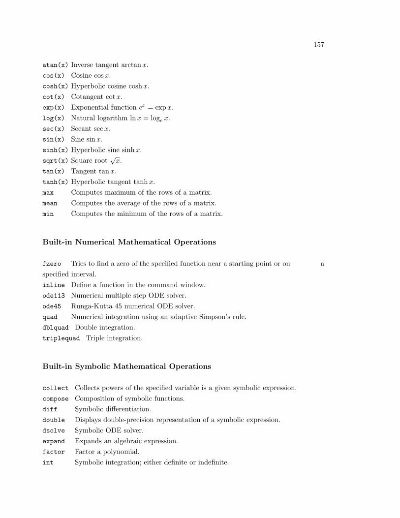
157

atan(x) Inverse tangent arctanx.

cos(x) Cosine cosx.

cosh(x) Hyperbolic cosine coshx.

cot(x) Cotangent cotx.

exp(x) Exponential function ex = expx.

log(x) Natural logarithm lnx = loge x.

sec(x) Secant secx.

sin(x) Sine sinx.

sinh(x) Hyperbolic sine sinhx.

sqrt(x) Square root√x.

tan(x) Tangent tanx.

tanh(x) Hyperbolic tangent tanhx.

max Computes maximum of the rows of a matrix.

mean Computes the average of the rows of a matrix.

min Computes the minimum of the rows of a matrix.

Built-in Numerical Mathematical Operations

fzero Tries to find a zero of the specified function near a starting point or on a

specified interval.

inline Define a function in the command window.

ode113 Numerical multiple step ODE solver.

ode45 Runga-Kutta 45 numerical ODE solver.

quad Numerical integration using an adaptive Simpson’s rule.

dblquad Double integration.

triplequad Triple integration.

Built-in Symbolic Mathematical Operations

collect Collects powers of the specified variable is a given symbolic expression.

compose Composition of symbolic functions.

diff Symbolic differentiation.

double Displays double-precision representation of a symbolic expression.

dsolve Symbolic ODE solver.

expand Expands an algebraic expression.

factor Factor a polynomial.

int Symbolic integration; either definite or indefinite.

158 APPENDIX B. GLOSSARY OF MATLAB COMMANDS

limit Finds two-sided limit, if it exists.

pretty Displays a symbolic expression in a nice format.

simple Simplifies a symbolic expression.

subs Substitutes for parts a a symbolic expression.

sym or syms Create symbolic variables.

symsum Performs a symbolic summation, possibly with infinitely many entries.

taylor Gives a Taylor polynomial approximation of a given order at a specified point.

Graphics Commands

contour Plots level curves of a function of two variables.

contourf Filled contour plot.

ezcontour Easy contour plot.

loglog Creates a log-log plot.

mesh Draws a mesh surface.

meshgrid Creates arrays that can be used as inputs in graphics commands

such as contour, mesh, quiver, and surf.

ezmesh Easy mesh surface plot.

plot Plots data vectors.

ezplot Easy plot for symbolic functions.

plot3 Plots curves in 3-D.

polar Plots in polar coordinates.

quiver Plots a vector field.

semilogy Semilog plot, with logarithmic scale along the vertical direction.

surf Solid surface plot.

trimesh Plot based on a triangulation trisurf Surface plot based on a triangulation

Special Matlab Commands

: Range operator, used for defining vectors and in loops. Type help colon

for information.

; Suppresses output. Also separates rows of a matrix.

= Assigns the variable on the left hand side the value of the right hand side.

ans The value of the most recent unassigned.

cd Change directory.

clear Clears all values and definitions of variables and functions. You may also use to

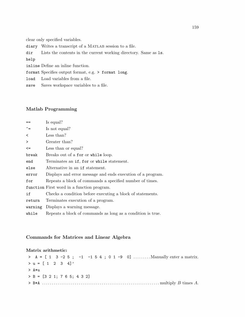
159

clear only specified variables.

diary Writes a transcript of a Matlab session to a file.

dir Lists the contents in the current working directory. Same as ls.

help

inline Define an inline function.

format Specifies output format, e.g. > format long.

load Load variables from a file.

save Saves workspace variables to a file.

Matlab Programming

== Is equal?

~= Is not equal?

< Less than?

> Greater than?

<= Less than or equal?

break Breaks out of a for or while loop.

end Terminates an if, for or while statement.

else Alternative in an if statement.

error Displays and error message and ends execution of a program.

for Repeats a block of commands a specified number of times.

function First word in a function program.

if Checks a condition before executing a block of statements.

return Terminates execution of a program.

warning Displays a warning message.

while Repeats a block of commands as long as a condition is true.

Commands for Matrices and Linear Algebra

Matrix arithmetic:

> A = [ 1 3 -2 5 ; -1 -1 5 4 ; 0 1 -9 0] . . . . . . . . .Manually enter a matrix.

> u = [ 1 2 3 4]’

> A*u

> B = [3 2 1; 7 6 5; 4 3 2]

> B*A . . . . . . . . . . . . . . . . . . . . . . . . . . . . . . . . . . . . . . . . . . . . . . . . . . . . . . . . . . . . . multiply B times A.

160 APPENDIX B. GLOSSARY OF MATLAB COMMANDS

> 2*A . . . . . . . . . . . . . . . . . . . . . . . . . . . . . . . . . . . . . . . . . . . . . . . . . . . .multiply a matrix by a scalar.

> A + A . . . . . . . . . . . . . . . . . . . . . . . . . . . . . . . . . . . . . . . . . . . . . . . . . . . . . . . . . . . . . . . . . .add matrices.

> A + 3 . . . . . . . . . . . . . . . . . . . . . . . . . . . . . . . . . . . . . . add a number to every entry of a matrix.

> B.*B . . . . . . . . . . . . . . . . . . . . . . . . . . . . . . . . . . . . . . . . . . . . . . . . . component-wise multiplication.

> B.^3 . . . . . . . . . . . . . . . . . . . . . . . . . . . . . . . . . . . . . . . . . . . . . . . . component-wise exponentiation.

Special matrices:

> I = eye(3) . . . . . . . . . . . . . . . . . . . . . . . . . . . . . . . . . . . . . . . . . . . . . . . . . . . . . . . . . . identity matrix

> D = ones(5,5)

> O = zeros(10,10)

> C = rand(5,5) . . . . . . . . . . . . . . . . . . . . random matrix with uniform distribution in [0, 1].

> C = randn(5,5) . . . . . . . . . . . . . . . . . . . . . . . . . . . random matrix with normal distribution.

> hilb(6)

> pascal(5)

General matrix commands:

> size(C) . . . . . . . . . . . . . . . . . . . . . . . . . . . . . . . . . . . . . . . . . . gives the dimensions (m× n) of A.

> norm(C) . . . . . . . . . . . . . . . . . . . . . . . . . . . . . . . . . . . . . . . . . . . . . . . gives the norm of the matrix.

> det(C) . . . . . . . . . . . . . . . . . . . . . . . . . . . . . . . . . . . . . . . . . . . . . . . the determinant of the matrix.

> max(C) . . . . . . . . . . . . . . . . . . . . . . . . . . . . . . . . . . . . . . . . . . . . . . . . . . . the maximum of each row.

> min(C) . . . . . . . . . . . . . . . . . . . . . . . . . . . . . . . . . . . . . . . . . . . . . . . . . . . . the minimum in each row.

> sum(C) . . . . . . . . . . . . . . . . . . . . . . . . . . . . . . . . . . . . . . . . . . . . . . . . . . . . . . . . . . . . . . . sums each row.

> mean(C) . . . . . . . . . . . . . . . . . . . . . . . . . . . . . . . . . . . . . . . . . . . . . . . . . . . . .the average of each row.

> diag(C) . . . . . . . . . . . . . . . . . . . . . . . . . . . . . . . . . . . . . . . . . . . . . . . . . . just the diagonal elements.

> inv(C) . . . . . . . . . . . . . . . . . . . . . . . . . . . . . . . . . . . . . . . . . . . . . . . . . . . . . . . . inverse of the matrix.

Matrix decompositions:

> [L U P] = lu(C)

> [Q R] = qr(C)

> [U S V] = svm(C) . . . . . . . . . . . . . . . . . . . . . . . . . . . . . . . . . . . . singular value decomposition.

Bibliography

[1] Ayyup and McCuen, 1996.

[2] E. Johnston, J. Mathews, Calculus, Addison-Wesley, 2001

161

GNU Free Documentation License

Version 1.3, 3 November 2008

Copyright c© 2000, 2001, 2002, 2007, 2008 Free Software Foundation, Inc.

<http://fsf.org/>

Everyone is permitted to copy and distribute verbatim copies of this license document,

but changing it is not allowed.

Preamble

The purpose of this License is to make a manual, textbook, or other functional and useful

document “free” in the sense of freedom: to assure everyone the effective freedom to copy

and redistribute it, with or without modifying it, either commercially or noncommercially.

Secondarily, this License preserves for the author and publisher a way to get credit for their

work, while not being considered responsible for modifications made by others.

This License is a kind of “copyleft”, which means that derivative works of the document

must themselves be free in the same sense. It complements the GNU General Public License,

which is a copyleft license designed for free software.

We have designed this License in order to use it for manuals for free software, because free

software needs free documentation: a free program should come with manuals providing the

same freedoms that the software does. But this License is not limited to software manuals;

it can be used for any textual work, regardless of subject matter or whether it is published

as a printed book. We recommend this License principally for works whose purpose is

instruction or reference.

1. APPLICABILITY AND DEFINITIONS

This License applies to any manual or other work, in any medium, that contains a notice

placed by the copyright holder saying it can be distributed under the terms of this License.

162

GNU Free Documentation License 163

Such a notice grants a world-wide, royalty-free license, unlimited in duration, to use that

work under the conditions stated herein. The “Document”, below, refers to any such

manual or work. Any member of the public is a licensee, and is addressed as “you”. You

accept the license if you copy, modify or distribute the work in a way requiring permission

under copyright law.

A “Modified Version” of the Document means any work containing the Document or a

portion of it, either copied verbatim, or with modifications and/or translated into another

language.

A “Secondary Section” is a named appendix or a front-matter section of the Document

that deals exclusively with the relationship of the publishers or authors of the Document

to the Document’s overall subject (or to related matters) and contains nothing that could

fall directly within that overall subject. (Thus, if the Document is in part a textbook of

mathematics, a Secondary Section may not explain any mathematics.) The relationship

could be a matter of historical connection with the subject or with related matters, or of

legal, commercial, philosophical, ethical or political position regarding them.

The “Invariant Sections” are certain Secondary Sections whose titles are designated, as

being those of Invariant Sections, in the notice that says that the Document is released

under this License. If a section does not fit the above definition of Secondary then it is not

allowed to be designated as Invariant. The Document may contain zero Invariant Sections.

If the Document does not identify any Invariant Sections then there are none.

The “Cover Texts” are certain short passages of text that are listed, as Front-Cover Texts

or Back-Cover Texts, in the notice that says that the Document is released under this

License. A Front-Cover Text may be at most 5 words, and a Back-Cover Text may be at

most 25 words.

A “Transparent” copy of the Document means a machine-readable copy, represented in

a format whose specification is available to the general public, that is suitable for revising

the document straightforwardly with generic text editors or (for images composed of pixels)

generic paint programs or (for drawings) some widely available drawing editor, and that

is suitable for input to text formatters or for automatic translation to a variety of formats

suitable for input to text formatters. A copy made in an otherwise Transparent file format

whose markup, or absence of markup, has been arranged to thwart or discourage subsequent

modification by readers is not Transparent. An image format is not Transparent if used for

any substantial amount of text. A copy that is not “Transparent” is called “Opaque”.

Examples of suitable formats for Transparent copies include plain ASCII without markup,

Texinfo input format, LaTeX input format, SGML or XML using a publicly available DTD,

164 GNU Free Documentation License

and standard-conforming simple HTML, PostScript or PDF designed for human modifica-

tion. Examples of transparent image formats include PNG, XCF and JPG. Opaque formats

include proprietary formats that can be read and edited only by proprietary word proces-

sors, SGML or XML for which the DTD and/or processing tools are not generally available,

and the machine-generated HTML, PostScript or PDF produced by some word processors

for output purposes only.

The “Title Page” means, for a printed book, the title page itself, plus such following pages

as are needed to hold, legibly, the material this License requires to appear in the title page.

For works in formats which do not have any title page as such, “Title Page” means the

text near the most prominent appearance of the work’s title, preceding the beginning of

the body of the text.

The “publisher” means any person or entity that distributes copies of the Document to

the public.

A section “Entitled XYZ” means a named subunit of the Document whose title ei-

ther is precisely XYZ or contains XYZ in parentheses following text that translates XYZ

in another language. (Here XYZ stands for a specific section name mentioned below,

such as “Acknowledgements”, “Dedications”, “Endorsements”, or “History”.) To

“Preserve the Title” of such a section when you modify the Document means that it

remains a section “Entitled XYZ” according to this definition.

The Document may include Warranty Disclaimers next to the notice which states that

this License applies to the Document. These Warranty Disclaimers are considered to be

included by reference in this License, but only as regards disclaiming warranties: any other

implication that these Warranty Disclaimers may have is void and has no effect on the

meaning of this License.

2. VERBATIM COPYING

You may copy and distribute the Document in any medium, either commercially or noncom-

mercially, provided that this License, the copyright notices, and the license notice saying

this License applies to the Document are reproduced in all copies, and that you add no

other conditions whatsoever to those of this License. You may not use technical measures

to obstruct or control the reading or further copying of the copies you make or distribute.

However, you may accept compensation in exchange for copies. If you distribute a large

enough number of copies you must also follow the conditions in section 3.

GNU Free Documentation License 165

You may also lend copies, under the same conditions stated above, and you may publicly

display copies.

3. COPYING IN QUANTITY

If you publish printed copies (or copies in media that commonly have printed covers) of the

Document, numbering more than 100, and the Document’s license notice requires Cover

Texts, you must enclose the copies in covers that carry, clearly and legibly, all these Cover

Texts: Front-Cover Texts on the front cover, and Back-Cover Texts on the back cover. Both

covers must also clearly and legibly identify you as the publisher of these copies. The front

cover must present the full title with all words of the title equally prominent and visible.

You may add other material on the covers in addition. Copying with changes limited to

the covers, as long as they preserve the title of the Document and satisfy these conditions,

can be treated as verbatim copying in other respects.

If the required texts for either cover are too voluminous to fit legibly, you should put the

first ones listed (as many as fit reasonably) on the actual cover, and continue the rest onto

adjacent pages.

If you publish or distribute Opaque copies of the Document numbering more than 100, you

must either include a machine-readable Transparent copy along with each Opaque copy,

or state in or with each Opaque copy a computer-network location from which the general

network-using public has access to download using public-standard network protocols a

complete Transparent copy of the Document, free of added material. If you use the latter

option, you must take reasonably prudent steps, when you begin distribution of Opaque

copies in quantity, to ensure that this Transparent copy will remain thus accessible at the

stated location until at least one year after the last time you distribute an Opaque copy

(directly or through your agents or retailers) of that edition to the public.

It is requested, but not required, that you contact the authors of the Document well before

redistributing any large number of copies, to give them a chance to provide you with an

updated version of the Document.

4. MODIFICATIONS

You may copy and distribute a Modified Version of the Document under the conditions

of sections 2 and 3 above, provided that you release the Modified Version under precisely

this License, with the Modified Version filling the role of the Document, thus licensing

166 GNU Free Documentation License

distribution and modification of the Modified Version to whoever possesses a copy of it. In

addition, you must do these things in the Modified Version:

A. Use in the Title Page (and on the covers, if any) a title distinct from that of the

Document, and from those of previous versions (which should, if there were any, be

listed in the History section of the Document). You may use the same title as a

previous version if the original publisher of that version gives permission.

B. List on the Title Page, as authors, one or more persons or entities responsible for

authorship of the modifications in the Modified Version, together with at least five

of the principal authors of the Document (all of its principal authors, if it has fewer

than five), unless they release you from this requirement.

C. State on the Title page the name of the publisher of the Modified Version, as the

publisher.

D. Preserve all the copyright notices of the Document.

E. Add an appropriate copyright notice for your modifications adjacent to the other

copyright notices.

F. Include, immediately after the copyright notices, a license notice giving the public

permission to use the Modified Version under the terms of this License, in the form

shown in the Addendum below.

G. Preserve in that license notice the full lists of Invariant Sections and required Cover

Texts given in the Document’s license notice.

H. Include an unaltered copy of this License.

I. Preserve the section Entitled “History”, Preserve its Title, and add to it an item

stating at least the title, year, new authors, and publisher of the Modified Version as

given on the Title Page. If there is no section Entitled “History” in the Document,

create one stating the title, year, authors, and publisher of the Document as given

on its Title Page, then add an item describing the Modified Version as stated in the

previous sentence.

J. Preserve the network location, if any, given in the Document for public access to

a Transparent copy of the Document, and likewise the network locations given in

the Document for previous versions it was based on. These may be placed in the

“History” section. You may omit a network location for a work that was published at

least four years before the Document itself, or if the original publisher of the version

it refers to gives permission.

GNU Free Documentation License 167

K. For any section Entitled “Acknowledgements” or “Dedications”, Preserve the Title

of the section, and preserve in the section all the substance and tone of each of the

contributor acknowledgements and/or dedications given therein.

L. Preserve all the Invariant Sections of the Document, unaltered in their text and in

their titles. Section numbers or the equivalent are not considered part of the section

titles.

M. Delete any section Entitled “Endorsements”. Such a section may not be included in

the Modified Version.

N. Do not retitle any existing section to be Entitled “Endorsements” or to conflict in

title with any Invariant Section.

O. Preserve any Warranty Disclaimers.

If the Modified Version includes new front-matter sections or appendices that qualify as

Secondary Sections and contain no material copied from the Document, you may at your

option designate some or all of these sections as invariant. To do this, add their titles to

the list of Invariant Sections in the Modified Version’s license notice. These titles must be

distinct from any other section titles.

You may add a section Entitled “Endorsements”, provided it contains nothing but endorse-

ments of your Modified Version by various parties—for example, statements of peer review

or that the text has been approved by an organization as the authoritative definition of a

standard.

You may add a passage of up to five words as a Front-Cover Text, and a passage of up

to 25 words as a Back-Cover Text, to the end of the list of Cover Texts in the Modified

Version. Only one passage of Front-Cover Text and one of Back-Cover Text may be added

by (or through arrangements made by) any one entity. If the Document already includes

a cover text for the same cover, previously added by you or by arrangement made by the

same entity you are acting on behalf of, you may not add another; but you may replace the

old one, on explicit permission from the previous publisher that added the old one.

The author(s) and publisher(s) of the Document do not by this License give permission to

use their names for publicity for or to assert or imply endorsement of any Modified Version.

5. COMBINING DOCUMENTS

You may combine the Document with other documents released under this License, under

the terms defined in section 4 above for modified versions, provided that you include in the

168 GNU Free Documentation License

combination all of the Invariant Sections of all of the original documents, unmodified, and

list them all as Invariant Sections of your combined work in its license notice, and that you

preserve all their Warranty Disclaimers.

The combined work need only contain one copy of this License, and multiple identical

Invariant Sections may be replaced with a single copy. If there are multiple Invariant

Sections with the same name but different contents, make the title of each such section

unique by adding at the end of it, in parentheses, the name of the original author or

publisher of that section if known, or else a unique number. Make the same adjustment to

the section titles in the list of Invariant Sections in the license notice of the combined work.

In the combination, you must combine any sections Entitled “History” in the various original

documents, forming one section Entitled “History”; likewise combine any sections Entitled

“Acknowledgements”, and any sections Entitled “Dedications”. You must delete all sections

Entitled “Endorsements”.

6. COLLECTIONS OF DOCUMENTS

You may make a collection consisting of the Document and other documents released under

this License, and replace the individual copies of this License in the various documents with

a single copy that is included in the collection, provided that you follow the rules of this

License for verbatim copying of each of the documents in all other respects.

You may extract a single document from such a collection, and distribute it individually

under this License, provided you insert a copy of this License into the extracted document,

and follow this License in all other respects regarding verbatim copying of that document.

7. AGGREGATION WITH INDEPENDENT WORKS

A compilation of the Document or its derivatives with other separate and independent

documents or works, in or on a volume of a storage or distribution medium, is called an

“aggregate” if the copyright resulting from the compilation is not used to limit the legal

rights of the compilation’s users beyond what the individual works permit. When the

Document is included in an aggregate, this License does not apply to the other works in

the aggregate which are not themselves derivative works of the Document.

If the Cover Text requirement of section 3 is applicable to these copies of the Document,

then if the Document is less than one half of the entire aggregate, the Document’s Cover

Texts may be placed on covers that bracket the Document within the aggregate, or the

GNU Free Documentation License 169

electronic equivalent of covers if the Document is in electronic form. Otherwise they must

appear on printed covers that bracket the whole aggregate.

8. TRANSLATION

Translation is considered a kind of modification, so you may distribute translations of the

Document under the terms of section 4. Replacing Invariant Sections with translations

requires special permission from their copyright holders, but you may include translations

of some or all Invariant Sections in addition to the original versions of these Invariant

Sections. You may include a translation of this License, and all the license notices in

the Document, and any Warranty Disclaimers, provided that you also include the original

English version of this License and the original versions of those notices and disclaimers.

In case of a disagreement between the translation and the original version of this License

or a notice or disclaimer, the original version will prevail.

If a section in the Document is Entitled “Acknowledgements”, “Dedications”, or “History”,

the requirement (section 4) to Preserve its Title (section 1) will typically require changing

the actual title.

9. TERMINATION

You may not copy, modify, sublicense, or distribute the Document except as expressly pro-

vided under this License. Any attempt otherwise to copy, modify, sublicense, or distribute

it is void, and will automatically terminate your rights under this License.

However, if you cease all violation of this License, then your license from a particular copy-

right holder is reinstated (a) provisionally, unless and until the copyright holder explicitly

and finally terminates your license, and (b) permanently, if the copyright holder fails to

notify you of the violation by some reasonable means prior to 60 days after the cessation.

Moreover, your license from a particular copyright holder is reinstated permanently if the

copyright holder notifies you of the violation by some reasonable means, this is the first

time you have received notice of violation of this License (for any work) from that copyright

holder, and you cure the violation prior to 30 days after your receipt of the notice.

Termination of your rights under this section does not terminate the licenses of parties

who have received copies or rights from you under this License. If your rights have been

terminated and not permanently reinstated, receipt of a copy of some or all of the same

material does not give you any rights to use it.

170 GNU Free Documentation License

10. FUTURE REVISIONS OF THIS LICENSE

The Free Software Foundation may publish new, revised versions of the GNU Free Doc-

umentation License from time to time. Such new versions will be similar in spirit to

the present version, but may differ in detail to address new problems or concerns. See

http://www.gnu.org/copyleft/.

Each version of the License is given a distinguishing version number. If the Document

specifies that a particular numbered version of this License “or any later version” applies

to it, you have the option of following the terms and conditions either of that specified

version or of any later version that has been published (not as a draft) by the Free Software

Foundation. If the Document does not specify a version number of this License, you may

choose any version ever published (not as a draft) by the Free Software Foundation. If the

Document specifies that a proxy can decide which future versions of this License can be

used, that proxy’s public statement of acceptance of a version permanently authorizes you

to choose that version for the Document.

11. RELICENSING

“Massive Multiauthor Collaboration Site” (or “MMC Site”) means any World Wide Web

server that publishes copyrightable works and also provides prominent facilities for anybody

to edit those works. A public wiki that anybody can edit is an example of such a server.

A “Massive Multiauthor Collaboration” (or “MMC”) contained in the site means any set

of copyrightable works thus published on the MMC site.

“CC-BY-SA” means the Creative Commons Attribution-Share Alike 3.0 license published

by Creative Commons Corporation, a not-for-profit corporation with a principal place of

business in San Francisco, California, as well as future copyleft versions of that license

published by that same organization.

“Incorporate” means to publish or republish a Document, in whole or in part, as part of

another Document.

An MMC is “eligible for relicensing” if it is licensed under this License, and if all works that

were first published under this License somewhere other than this MMC, and subsequently

incorporated in whole or in part into the MMC, (1) had no cover texts or invariant sections,

and (2) were thus incorporated prior to November 1, 2008.

The operator of an MMC Site may republish an MMC contained in the site under CC-BY-

SA on the same site at any time before August 1, 2009, provided the MMC is eligible for

GNU Free Documentation License 171

relicensing.

ADDENDUM: How to use this License for your documents

To use this License in a document you have written, include a copy of the License in the

document and put the following copyright and license notices just after the title page:

Copyright c© YEAR YOUR NAME. Permission is granted to copy, distribute

and/or modify this document under the terms of the GNU Free Documenta-

tion License, Version 1.3 or any later version published by the Free Software

Foundation; with no Invariant Sections, no Front-Cover Texts, and no Back-

Cover Texts. A copy of the license is included in the section entitled “GNU

Free Documentation License”.

If you have Invariant Sections, Front-Cover Texts and Back-Cover Texts, replace the “with

. . . Texts.” line with this:

with the Invariant Sections being LIST THEIR TITLES, with the Front-Cover

Texts being LIST, and with the Back-Cover Texts being LIST.

If you have Invariant Sections without Cover Texts, or some other combination of the three,

merge those two alternatives to suit the situation.

If your document contains nontrivial examples of program code, we recommend releasing

these examples in parallel under your choice of free software license, such as the GNU

General Public License, to permit their use in free software.