HAL Id: cel-01484274https://hal.archives-ouvertes.fr/cel-01484274

Submitted on 7 Mar 2017

HAL is a multi-disciplinary open accessarchive for the deposit and dissemination of sci-entific research documents, whether they are pub-lished or not. The documents may come fromteaching and research institutions in France orabroad, or from public or private research centers.

L’archive ouverte pluridisciplinaire HAL, estdestinée au dépôt et à la diffusion de documentsscientifiques de niveau recherche, publiés ou non,émanant des établissements d’enseignement et derecherche français ou étrangers, des laboratoirespublics ou privés.

Introduction to numerical methods for OrdinaryDifferential Equations

Charles-Edouard Bréhier

To cite this version:Charles-Edouard Bréhier. Introduction to numerical methods for Ordinary Differential Equations.Licence. Introduction to numerical methods for Ordinary Differential Equations, Pristina, Kosovo,Serbia. 2016. �cel-01484274�

Introduction to numerical methods for OrdinaryDifferential Equations

C. -E. Bréhier

November 14, 2016

AbstractThe aims of these lecture notes are the following.

• We introduce Euler numerical schemes, and prove existence and uniqueness ofsolutions of ODEs passing to the limit in a discretized version.

• We provide a general theory of one-step integrators, based on the notions of sta-bility and consistency.

• We propose some procedures which lead to construction of higher-order methods.• We discuss splitting and composition methods.• We finally focus on qualitative properties of Hamiltonian systems and of their

discretizations.

Good references, in particular for integration of Hamiltonian systems, are the mono-graphs Geometric Numerical Integration, by E. Hairer, C. Lubich and G. Wan-ner, and Molecular Dynamics. With deterministic and stochastic numericalmethods., by B. Leimkuhler and C. Matthews.

Contents1 Ordinary Differential Equations 3

1.1 Well-posedness theory . . . . . . . . . . . . . . . . . . . . . . . . . . . . . . 31.2 Some important examples . . . . . . . . . . . . . . . . . . . . . . . . . . . . 6

1.2.1 Linear ODEs . . . . . . . . . . . . . . . . . . . . . . . . . . . . . . . 61.2.2 Gradient dynamics . . . . . . . . . . . . . . . . . . . . . . . . . . . . 61.2.3 Hamiltonian dynamics . . . . . . . . . . . . . . . . . . . . . . . . . . 71.2.4 Examples of potential energy functions . . . . . . . . . . . . . . . . . 71.2.5 The Lotka-Volterra system . . . . . . . . . . . . . . . . . . . . . . . . 8

2 Euler schemes 102.1 The explicit Euler scheme . . . . . . . . . . . . . . . . . . . . . . . . . . . . 102.2 The implicit Euler scheme . . . . . . . . . . . . . . . . . . . . . . . . . . . . 122.3 The θ-scheme . . . . . . . . . . . . . . . . . . . . . . . . . . . . . . . . . . . 13

1

3 General analysis of one-step integrators 143.1 One-step integrators . . . . . . . . . . . . . . . . . . . . . . . . . . . . . . . 143.2 Stability . . . . . . . . . . . . . . . . . . . . . . . . . . . . . . . . . . . . . . 143.3 Consistency . . . . . . . . . . . . . . . . . . . . . . . . . . . . . . . . . . . . 163.4 Convergence . . . . . . . . . . . . . . . . . . . . . . . . . . . . . . . . . . . . 183.5 Long-time behavior: A-stability . . . . . . . . . . . . . . . . . . . . . . . . . 19

4 Some constructions of higher-order methods 204.1 Taylor expansions . . . . . . . . . . . . . . . . . . . . . . . . . . . . . . . . . 204.2 Quadrature methods for integrals . . . . . . . . . . . . . . . . . . . . . . . . 204.3 A few recipes . . . . . . . . . . . . . . . . . . . . . . . . . . . . . . . . . . . 22

4.3.1 Removing derivatives . . . . . . . . . . . . . . . . . . . . . . . . . . . 224.3.2 Removing implicitness . . . . . . . . . . . . . . . . . . . . . . . . . . 23

4.4 Runge-Kutta methods . . . . . . . . . . . . . . . . . . . . . . . . . . . . . . 234.5 Order of convergence and cost of a method . . . . . . . . . . . . . . . . . . . 24

5 Splitting and composition methods 265.1 Splitting methods . . . . . . . . . . . . . . . . . . . . . . . . . . . . . . . . . 265.2 The adjoint of an integrator . . . . . . . . . . . . . . . . . . . . . . . . . . . 285.3 Composition methods . . . . . . . . . . . . . . . . . . . . . . . . . . . . . . . 295.4 Conjugate methods, effective order, processing . . . . . . . . . . . . . . . . . 29

6 Integrators for Hamiltonian dynamics 316.1 The Störmer-Verlet method . . . . . . . . . . . . . . . . . . . . . . . . . . . 31

6.1.1 A derivation of the Störmer-Verlet scheme . . . . . . . . . . . . . . . 326.1.2 Formulations for general Hamiltonian functions . . . . . . . . . . . . 32

6.2 Conservation of the Hamiltonian . . . . . . . . . . . . . . . . . . . . . . . . . 336.3 Symplectic mappings . . . . . . . . . . . . . . . . . . . . . . . . . . . . . . . 346.4 Symplectic integrators . . . . . . . . . . . . . . . . . . . . . . . . . . . . . . 356.5 Preservation of a modified Hamiltonian for the Störmer-Verlet scheme . . . . 36

7 Conclusion 37

8 Numerical illustration: the harmonic oscillator 38

2

1 Ordinary Differential EquationsThe main objective of these lecture notes is to present simulatable approximations of solu-tions of Ordinary Differential Equations (ODEs) of the form

x′ = F (x) (1)

where F : Rd → Rd is a vector field, and d ∈ N?. The minimal assumption on F iscontinuity; however well-posedness requires stronger conditions, in terms of (local) Lipschitzcontinuity.

We recall what we mean by a solution of (1).

Definition 1.1. Let T ∈ (0,+∞); a solution of (1) on the interval [0, T ] is a mappingx : [0, T ]→ Rd, of class C1, such that for every t ∈ [0, T ], x′(t) = F

(x(t)

).

We also recall the definition of a Lipschitz continuous function.

Definition 1.2. Let F : Rd → Rd.F is globally Lipschitz continuous if there exists LF ∈ (0,+∞) such that for every x1, x2 ∈

Rd

‖F (x2)− F (x1)‖ ≤ LF‖x2 − x1‖.

F is locally Lipschitz continuous if, for every R ∈ (0,+∞), there exists LF (R) ∈ (0,+∞)such that for every x1, x2 ∈ Rd, with max

(‖x1‖, ‖x2‖

)≤ R,

‖F (x2)− F (x1)‖ ≤ LF (R)‖x2 − x1‖.

1.1 Well-posedness theory

In order to deal with solutions of (1), we first need to study well-posedness of the Cauchyproblem:

x′ = F (x) , x(0) = x0, (2)

where x0 ∈ Rd is an initial condition.The Cauchy problem is globally well-posed in the sense of Hadamard if, firstly, for

every T ∈ (0,+∞), there exists a unique solution x of (1) on [0, T ], such that x(0) = x0;and if, secondly, the solution depends continuously on the initial condition x0.

Assuming the global Lipschitz continuity of F provides global well-posedness: this is thecelebrated Cauchy-Lipschitz theorem. If one only assumes that F is locally Lipschitzcontinuous, well-posedness is only local: the existence time T may depend on the initialcondition x0. However, there are criteria ensuring global existence of solutions. Finally, if Fis only assumed to be continuous, uniqueness may not be satisfied; however existence maybe proven (this is the Cauchy-Peano theorem), using the strategy presented below (and anappropriate compactness argument). Such situations are not considered in these notes.

3

Theorem 1.3 (Cauchy-Lipschitz). Assume that F is (globally) Lipschitz continuous. Thenthe Cauchy problem is well-posed in the sense of Hadamard: for every T ∈ (0,+∞) andevery x0 ∈ Rd, there exists a unique x solution of (2).

Then let φ : [0,+∞) × Rd → Rd, defined by φ(t, x0) = x(t). There exists C ∈ (0,+∞),such that, for every T ∈ (0,+∞), and every x1, x2 ∈ Rd

supt∈[0,T ]

‖φ(t, x1)− φ(t, x2)‖ ≤ exp(CT)‖x1 − x2‖.

The mapping φ is called the flow of the ODE. The following notation is often used:φt = φ(t, ·), for every t ≥ 0. Thanks to the Cauchy-Lipschitz Theorem 1.3, for every t, s ≥ 0,

φt+s = φt ◦ φs. (3)

This important equality is the flow property (or the semigroup property).Note that if F is of class Ck for some k ∈ N?, then the flow is also of class Ck, i.e. Φt is

of class Ck for every t ≥ 0. We do not prove this result in these notes.The key tool to prove all the results in Theorem 1.3 (as well as many other results) is

the celebrated Gronwall’s Lemma.

Lemma 1.4 (Gronwall’s Lemma). Let T ∈ (0,+∞), and θ : [0, T ]→ [0,+∞) a continuous,nonnegative, function.

Assume that there exists α ∈ [0,+∞) and β ∈ (0,+∞) such that for every t ∈ [0, T ]

θ(t) ≤ α + β

∫ t

0

θ(s)ds.

Then θ(t) ≤ α exp(βT ) for every t ∈ [0, T ].

Proof of Gronwall’s Lemma. The mapping t ∈ [0, T ] 7→ α+β∫ t0 θ(s)ds

αeβtis of class C1, non-

increasing (its derivative is nonpositive), and is equal to 1 at t = 0.

We are now in position to prove Theorem (1.3). To simplify the presentation, in additionto the global Lipschitz condition, we assume that F is bounded: there exists M ∈ (0,+∞)such that ‖F (x)‖ ≤M for every x ∈ Rd.

The standard proof of the Cauchy-Lipschitz theorem exploits the Picard iteration pro-cedure, or the Banach fixed point theorem. Here we present a different proof, where weconstruct approximate solutions by means of a numerical scheme; this strategy can be gen-eralized to prove the Cauchy-Peano Theorem, assuming only that F is continuous. Theproof presented here also supports the fact that numerical approximation may also be a niceapproach in theoretical problems.

Proof of Cauchy-Lipschitz theorem. 1. Uniqueness: let x1, x2 denote two solutions on [0, T ].Then for every t ∈ [0, T ]

‖x1(t)− x2(t)‖ =∥∥∫ t

0

(F (x1(s))− F (x2(s))

)ds∥∥ ≤ LF

∫ t

0

‖x1(s)− x2(s)‖ds,

4

where we have used x1(0) = x0 = x2(0), and Lipschitz continuity of F .

The conclusion follows from Gronwall’s Lemma: ‖x1(t)−x2(t)‖ ≤ 0 for every t ∈ [0, T ].

2. Existence: we construct a sequence of approximate solutions by means of a numericalscheme; we then prove (uniform) convergence of the sequence, and prove that the limitis solution of (1).

Let N ∈ N?, and denote h = T2N

, and tn = nh for every n ∈{

0, 1, . . . , 2N}.

Define

xN(t0) = x0,

xN(tn+1) = xN(tn) + hF (xN(tn)), n ∈{

0, 1, . . . , 2N − 1},

xN(t) =(tn+1 − t)tn+1 − tn

xN(tn) +(t− tn)

tn+1 − tnxN(tn+1), t ∈ [tn, tn+1], n ∈

{0, 1, . . . , 2N − 1

}.

(4)The initial condition for xN is x0 and does not depend on N . The second line definesxN(tn) recursively, for n ∈

{0, 1, . . . , 2N − 1

}. Finally, the third line defines a continu-

ous function xN : [0, T ]→ Rd by linear interpolation. Note that xN is continuous, andis moreover differentiable, except at points tn (where left and right derivatives exist).

Let n ∈{

0, 1, . . . , 2N − 1}. Then

‖(xN)′(t)‖ =‖xN(tn+1)− xN(tn)‖

h= ‖F (xN(tn))‖ ≤M

for every t ∈ (tn, tn+1), and thus ‖xN(t)− xN(tn)‖ ≤M(t− tn) ≤Mh.

This yields ‖(xN)′(t) − F (xN(t))‖ = ‖F (xN(t)) − F (xN(tn))‖ ≤ LFMh, for everyt ∈ (tn, tn+1). By subdividing the interval [0, t] as ∪

0≤k≤K−1[tk, tk+1) ∪ [tK , t], with K

such that tK ≤ t < tK+1, and integrating, for every t ∈ [0, T ]

‖xN(t)− x0 −∫ t

0

F (xN(s))ds‖ ≤ LFMth. (5)

Now let zN = xN+1 − xN . Then, using the triangle inequality,

‖zN(t)‖ = ‖xN+1(t)− xN(t)‖

≤ ‖∫ t

0

F (xN+1(s))ds−∫ t

0

F (xN(s))ds‖

+ ‖xN+1(t)− x0 −∫ t

0

F (xN+1(s))ds‖+ ‖xN(t)− x0 −∫ t

0

F (xN(s))ds‖

≤ LF

∫ t

0

‖zN(s)‖ds+ 2LFMT 2

2N.

5

Thanks to Gronwall’s Lemma, sup0≤t≤T

‖xN+1(t)− xN(t)‖ ≤ 2LFMT 2

2N.

We deduce that for every t ∈ [0, T ], the series∑

N∈N(xN+1(t) − xN(t)

)converges;

moreover, the convergence is uniform. Define x(t) =∑+∞

N=0

(xN+1(t)− xN(t)

)+ x0(t).

Note that x : [0, T ] → Rd is continuous, as the uniform limit of continuous functions.Moreover, x(t) = lim

N→+∞xN(t) (telescoping sum argument).

Since F is continuous, we can pass to the limit N → +∞ in the left-hand side of (5);since h = T2−N , we get the equality

x(t) = x0 +

∫ t

0

F (x(s))ds

for every t ∈ [0, T ], which is equivalent to (1). This concludes the proof of the existenceresult.

3. Lipschitz continuity of the flow: if x1, x2 ∈ Rd, by the triangle inequality

‖φt(x1)− φt(x2)‖ ≤ ‖x1 − x2‖+

∫ t

0

‖F (φs(x1))− F (φs(x2))‖ds,

for every t ∈ [0, T ]. Thanks to Lipschitz continuity of F and Gronwall’s Lemma, weget

sup0≤t≤T

‖φt(x1)− φt(x2)‖ ≤ eLFT‖x1 − x2‖.

1.2 Some important examples

1.2.1 Linear ODEs

If F (x) = Ax for every x ∈ Rd, where A is a d× d real-valued matrix, then for every t ≥ 0and every x0 ∈ Rd, one has

φt(x0) = etAx0,

where etA =∑+∞

n=0tn

n!An is the exponential of the matrix tA.

Properties of theses ODEs can be studied by choosing an appropriate representative B,such that B = P−1AP for some invertible matrix P .

For instance, if A can be diagonalized, it is straightforward to provide explicit solutionsof the ODE, in terms of the eigenvalues and of the eigenvectors.

1.2.2 Gradient dynamics

Let V : Rd → R be of class C2. V is called the potential energy function.

6

The gradient dynamics corresponds to the choice F (x) = −∇V (x):

x′ = −∇V (x).

Without further assumptions on the growth of V , solutions are a priori only local, but theysatisfy the inequality V

(x(t)

)≤ V

(x(0)

): indeed,

dV(x(t)

)dt

= −‖∇V(x(t)

)‖2 ≤ 0.

If for every r ∈ R, the level set{x ∈ Rd ; V (x) ≤ r

}is compact, then solutions are global.

The compact level set condition is satisfied for instance if there exists c, R ∈ (0,+∞) suchthat ‖V (x)‖ ≥ c‖x‖2 when ‖x‖ ≥ R.

Note that a linear ODE, F (x) = Ax, corresponds to a gradient dynamics if and only ifA is symmetric (Schwarz relations). In that case, A = −D2V (x) (the Hessian matrix) forevery x ∈ Rd, and V (x) = −1

2〈x,Ax〉. The level sets are compact if and only if −A only has

nonnegative eigenvalues.

1.2.3 Hamiltonian dynamics

Let H : Rd × Rd → R be of class C2. H is called the Hamiltonian function.The Hamiltonian dynamics is given by the ODE{

q = ∇pH(q, p)

p = −∇qH(q, p)

where we used the standard notation q and p to represent the time derivative.The typical example from mechanics is given by the total energy function H(q, p) =

‖p‖22

+ V (q), where q ∈ Rd represents the position, p ∈ Rd represents the momentum. Thetotal enery function is the sum of the kinetic energy ‖p‖

2

2and of the potential energy V (q).

The Hamiltonian dynamics is then given by

q = p , p = −∇V (q)

which can be rewritten as a second-order ODE: q = −∇V (q).One of the remarkable properties of Hamiltonian dynamics is the preservation of the

Hamiltonian function: if t 7→(q(t), p(t)

)is a local solution, thenH

(q(t), p(t)

)= H

(q(0), p(0)

).

If for every H0 ∈ R, the level set{

(q, p) ∈ R2d ; H(q, p) = H0

}is compact, then solutions

are global.

1.2.4 Examples of potential energy functions

The first example of potential function corresponds to the so-called harmonic oscillator (whenconsidering the associated Hamiltonian system): V (q) = ω2

2q2. The equation is linear, this

gives a good toy model to test properties of numerical methods.

7

The harmonic oscillator models a linear pendulum: a nonlinear example is given byV (q) = ω2(1− cos(q)), which gives −V ′(q) = −ω2 sin(q).

Even if the case of harmonic oscillators might seem very simple, chains of oscillatorsmight be challenging in presence of slow and fast oscillations.

For instance, for ω large, consider a chain of 2m+2 oscillators with Hamiltonian function

H(q1, . . . , q2m+1, p1, . . . , p2m+1

)=

2m∑i=1

p2i +

m∑i=1

ω2

2(q2i − q2i−1)2 +

m∑i=0

1

2(q2i+1 − q2i)

2,

with q0 = q2m+1 = 0 by convention, where stiff (frequency ω) and nonstiff (frequency 1)springs are alternated, and q1, . . . , q2m indicate displacements with respect to equilibriumpositions of springs. This is an example called the Fermi-Pasta-Ulam model.

In general, systems of ODEs with multiple time scales (stiff springs evolve at a fast timescale and nonstiff springs evolve at a slow time scale) require the use of specific multiscalemethods. This is still an active research area.

When studying systems with a large number of particles (molecular dynamics) orplanets (celestial mechanics), it is natural to consider potential energy functions whichare the sums of internal and pairwise interaction terms:

V (q) =L∑i=1

Vi(qi) +∑

1≤i<j≤L

Vij(qi, qj).

Typically, homogeneous interactions are considered: Vij(qi, qj) is a function Vij(qj − qi) ofqj − qi.

In celestial mechanics, with d = 3, typically Vi(q) = −GMmi‖q‖ and Vij(qi, qj) = −Gmimj

‖qi−qj‖ ,where mi is the mass of planet i and M is the (large) mass of another planet or star, andG > 0 is a physical parameter.

In molecular dynamics, a popular example is given by the Lennard-Jones potential

Vij(qi, qj) = 4εij

( σ12ij

‖qj − qi‖12−

σ6ij

‖qj − qi‖6

).

The force is repulsive for short distances, and attractive for sufficiently large distances.Both the examples in celestial mechanics and the molecular dynamics are challenging, in

particular due to the singularity of the potential functions at 0, and to the chaotic behaviorthey induce.

1.2.5 The Lotka-Volterra system

The Lotka-Volterra system is a popular predator-prey model: if u(t), resp. v(t), is the sizeof the population of predators, resp. of preys, at time t, the ODE system is given by

u = u(v − 2) , v = v(1− u),

8

where the values 2 and 1 are chosen arbitrarily.A first integral of the system is given by I(u, v) = ln(u) − u + 2 ln(v) − v: this means

that I is invariant by the flow, equivalently ddtI(u(t), v(t)) = 0.

This property is important, since it implies that the trajectories lie on level sets of I, andthat in fact solutions of the ODE are periodic.

It would be desirable to have numerical methods which do not destroy too much this niceproperty.

The conservation of I is not surprising: setting p = ln(u) and q = ln(v), and H(q, p) =I(eq, ep) = p − ep + 2q − eq, the Lotka-Volterra system is transformed into an Hamiltoniansystem. In other words, the flow of the Lotka-Volterra system is conjugated (via the changeof variables) to an Hamiltonian flow.

We will see later on nice integrators for Hamiltonian dynamics: they naturally yield niceintegrators for the Lotka-Volterra system.

9

2 Euler schemesThe proof of the existence part of Theorem 1.3 used the construction of approximate solu-tions, by means of a numerical method, see (4).

The principle was as follows: if t 7→ x(t) is differentiable at time t0, then x′(t) =

limh→0

x(t+h)−x(t)h

. In other words, x(t + h) = x(t) + hx′(t) + o(h). If x is solution of (1),then x′(t) = F (x(t)).

Neglecting the o(h) term leads to the definition of a recursion of the form

xhn+1 = xhn + hF (xhn).

This sequence is well-defined provided that an initial condition xh0 is given. Moreover, thecondition to have a simulatable sequence is that F (x) can be computed for every x ∈ Rd.

It is natural to assume that h = TN, where N ∈ N? is an integer. For n ∈ {0, . . . , N}, xhn

is an approximation of x(nh), the value of the exact solution at time tn = nh.Note that in the proof of Theorem 1.3, we have considered the case h = T2−N , in order

to easily set up the telescoping sum argument.

2.1 The explicit Euler scheme

The explicit Euler scheme (also called the forward Euler scheme), with time-step size h,associated with the Cauchy problem (2) is given by

xh0 = x0 , xhn+1 = xhn + hF (xhn). (6)

We prove the following result:

Theorem 2.1. Let T ∈ (0,+∞), and consider the explicit Euler scheme (6) with time stepsize h = T

N, with N ∈ N?.

Assume that the vector field F is bounded and Lipschitz continuous.Then there exist c, C ∈ (0,+∞) such that for every N ∈ N,

sup0≤n≤N

‖x(tn)− xhn‖ ≤ ecTh,

where x is the unique solution of (2).

We give two different detailed proofs, even if we give a more general statement belowwhich includes the case of the explicit Euler scheme. The first proof is similar to the computa-tions in the proof of Theorem 1.3. The second proof allows us to exhibit the two fundamentalproperties of numerical schemes which will be studied below: stability and consistency.

First proof of Theorem 2.1. Let tn = nh, for n ∈ N.

10

Introduce the right-continuous, piecewise linear, respectively the piecewise constant, in-terpolations of the sequence

(xhn)n≥0

: define for t ∈ [tn, tn+1), n ∈ N,

xh(t) =tn+1 − ttn+1 − tn

xhn +t− tn

tn+1 − tnxhn+1

xh(t) = xhn.

Then xh(t) = x0 +∫ t

0F(xh(s)

)ds.

Note also that, for every n ∈ N and t ∈ [tn, tn+1], ‖xh(t)− xh(t)‖ ≤ ‖xhn+1 − xhn‖ ≤Mh.Let εh(t) = x(t)− xh(t), where x is the solution of (2). Then for every t ∈ [0, T ],

‖εh(t)‖ ≤∫ t

0

‖F(x(s)

)− F

(xh(s)

)‖ds

≤∫ t

0

‖F(xh(s)

)− F

(xh(s)

)‖ds+

∫ t

0

‖F(x(s)

)− F

(xh(s)

)‖ds

≤ LFMh+ LF

∫ t

0

‖εh(s)‖ds.

By Gronwall’s Lemma, supt∈[0,T ]

‖εh(t)‖ ≤ LFMheLFT .

Second proof of Theorem 2.1. For every n ∈ N, define ehn = x(tn+1)− x(tn)− hF(x(tn)

).

Note that for t ∈ [tn, tn+1], ‖x(t)− x(tn)‖ ≤∫ ttn‖F(x(s)

)‖ds ≤Mh. As a consequence,

‖ehn‖ = ‖∫ tn+1

tn

(F(x(s)

)− F (xhn)

)ds‖ ≤ LFMh2.

Let also εhn = x(tn)− xhn. Then‖εhn+1‖ = ‖x(tn+1)− xhn+1‖

= ‖x(tn) + hF(x(tn)

)+ ehn − xhn − hF

(xhn)‖

≤ ‖ehn‖+(1 + LFh

)‖εhn‖

≤ LFMh2 +(1 + LFh

)‖εhn‖.

Dividing both sides by (1 + LFh)n+1 gives

‖εhn+1‖(1 + LFh)n+1

≤ ‖εhn‖(1 + LFh)n

+LFMh2

(1 + LFh)n+1,

which yields by a telescoping sum argument (since εh0 = 0)

‖εhn‖ ≤ LFMh2

n−1∑k=0

(1 + LFh)n−1−k

≤ LFMh2 (1 + LFh)n − 1

LFh

≤ eLFTMh.

11

2.2 The implicit Euler scheme

Before we focus on the general analysis of one-step numerical methods, we introduce theimplicit Euler scheme, as an alternative to the explicit Euler scheme.

Let λ > 0, and consider the linear ODE on R

x = −λx.

Given x0 ∈ R, obviously φt(x0) = e−λtx0. In particular:

• if x0 > 0, then φt(x0) > 0 for every t > 0;

• φt(x0) →t→+∞

0, for every x0 ∈ R.

Are these properties satisfied by the explicit Euler scheme with time-step h, when appliedin this simple linear situation?

Thanks to (6), one easily sees that xhn =(1− λh)nx0.

On the one hand, the positivity property is thus only satisfied if λh < 1: thus the time-step h needs to be sufficiently small. On the other hand,

(xhn)n∈N is bounded if and only if

|1− λh| ≤ 1, i.e. λh ≤ 2; and xhn →n→+∞

0 if and only if λh < 2.

The conditions h < λ−1 and h < 2λ−1 are very restrictive when λ is large.The alternative to recover stability properties is to use the backward Euler approximation.

It is based on writing the Taylor expansion x(t) = x(t − h) + hx′(t) + o(h), which leads tothe following scheme in the linear case:

xhn+1 = xhn − hλxhn+1.

The solution writes xhn = 1(1+λh)n

x0, and both positivity and asymptotic convergence prop-erties of the exact solution are preserved by the numerical scheme, whatever h > 0.

In the general case, the implicit Euler scheme, also called the backward Euler scheme,with time-step size h is defined by

xhn+1 = xhn + hF(xhn+1

). (7)

Since at each iteration the unknown xhn+1 appears on both sides of the equation (7), thescheme is implicit, and often the equation cannot be solved explicitly. For instance, one mayuse the Newton method to compute approximate values.

Moreover, the fact that there exists a unique solution y to the equation y = x+hF (y), forevery x ∈ Rd, may not be guaranteed in general. However, we have the following criterion,which requires again h to be small enough.

Proposition 2.2. Assume that hLF < 1. Then, for every x ∈ Rd, there exists a uniquesolution y(x) to the equation y = x+ hF (y).

Moreover, x 7→ y(x) is Lipchitz continuous, and ‖y(x2)− y(x1)‖ ≤ 11−hLF

‖x2 − x1‖.

12

Proof. • Uniqueness: if y = x+ hF (y) and z = x+ hF (z) are two solutions, then

‖y − z‖ = h‖F (y)− F (z)‖ ≤ hLF‖y − z‖,

which implies ‖y − z‖, and thus y = z.

• Existence: let x ∈ Rd, and consider an arbitrary y0 ∈ Rd. Define yk+1 = x+ hF (yk).

Then ‖yk+1 − yk‖ ≤ hLF‖yk − yk−1‖ ≤ . . . ≤(hLF

)k‖y1 − y0‖, for every k ∈ N.

Since Rd is a complete metric space, we can define y∞ = y0 +∑+∞

k=0

(yk+1 − yk

)=

limk→+∞

yk.

Passing to the limit k → +∞ in the equation yk+1 = x + hF (yk), we get y∞ =x+ hF (y∞). This gives the existence of a solution y∞.

• Lipschitz continuity: let x2, x1 ∈ Rd. Then(1−hLF

)‖y(x2)−y(x1)‖ ≤

(‖x2−x1‖+hLF‖y(x2)−y(x1)‖

)−hLF‖y(x2)−y(x1)‖ ≤ ‖x2−x1‖,

and one concludes using 1− hLF > 0.

In the case of the linear equation x = −λx, with λ > 0, no such condition is required:positivity of λ guarantees the well-posedness of the scheme.

An implicit scheme may then provide nice stability properties, but may be difficult tobe applied in practice for nonlinear problems. It is often a good strategy to provide semi-implicit schemes: a linear part is treated implicitly, and a nonlinear part is treated explicitly,see the example at the beginning of Section 5

2.3 The θ-scheme

The explicit and the implicit Euler schemes belong to the family of θ-method: let θ ∈ [0, 1],then the θ-scheme is defined as follows:

xθ,hn+1 = xθ,hn + (1− θ)hF(xθ,hn)

+ θhF(xθ,hn+1

). (8)

The case θ = 0 gives the explicit Euler scheme, whereas the case θ = 1 gives the implicitEuler scheme.

As soon as θ > 0, the θ-scheme (8) is not explicit.Choosing θ = 1/2, gives a popular method: the Crank-Nicolson scheme

xhn+1 = xhn +h

2

(F(xhn)

+ F(xhn+1

)). (9)

13

3 General analysis of one-step integrators

3.1 One-step integrators

Let h denote a time-step size.We consider numerical methods which have the form

xhn+1 = Φh(xhn). (10)

Such schemes are referred to as one-step integrators, or simply as integrators.The terminology “one-step integrator” refers to the fact that the computation of the

position xhn+1, at time n + 1, only requires to know the position xhn, at time n. Higher-order recursions xhn+1 = Φh(x

hn, x

hn−1, x

hn−m+1) are referred to as “multi-step methods” in the

literature.In the sequel, the following notation is useful: for h > 0, let Ψh(x) = 1

h

(Φh(x)− x

). We

assume that Ψ0(x) = limh→0

Ψh(x) is also well-defined, for every x ∈ Rd. We will also sometimesassume that Φh is also defined for h < 0.

Note that xn = Φnh(x0), where Φn

h denotes the composition Φh ◦ Φn−1h . The sequence(

Φnh

)0≤n≤N is often called the numerical flow: indeed, a semi-group property Φn+m

h =Φnh ◦ Φm

h is also satisfied, with integers n and m.

3.2 Stability

The first notion is the stability of a numerical scheme.

Definition 3.1. Let T ∈ (0,+∞), and consider an integrator Φh.The scheme (10) is stable on the interval [0, T ] if there exists h? > 0 and C ∈ (0,+∞),

such that if h = TN, with N ≥ N? > T

h?, then for any sequence

(ρn)

0≤n≤N in Rd, the sequence(yn)

0≤n≤N defined by the recursion,

yn+1 = Φh(yn) + ρn, (11)

satisfies the following inequality: for every n ∈ {0, . . . , N},

‖yn − xhn‖ ≤ C(‖y0 − xh0‖+

n−1∑m=0

‖ρm‖). (12)

The following sufficient condition for stability holds true.

Proposition 3.2. Assume that there exists L ∈ (0,+∞) and h? > 0 such that, for everyh ∈ (0, h?),

• Φh(x) = x+ hΨh(x) for every x ∈ Rd;

• ‖Ψh(x2)−Ψh(x1)‖ ≤ L‖x2 − x1‖ for every x1, x2 ∈ Rd.

14

Then the scheme (10) is stable on any interval [0, T ], with C = eLT .

Note that C = eLT →T→+∞

+∞: if the size of the interval is not fixed, the result of theproposition is not sufficient to establish a relationship between the asymptotic behaviors ofthe solution of the ODE (T → +∞) and of its numerical approximation (N → +∞). Forinstance, this is the situation described by the linear example x = −λx, with λ > 0.

Proof. The proof follows from arguments similar to the second proof of Theorem 2.1.Indeed,

‖yn+1 − xhn+1‖ ≤ ‖ρn‖+ ‖yn − xhn‖+ h‖Ψh(yn)−Ψh(xhn)‖

≤ ‖ρn‖+(1 + Lh

)‖yn − xhn‖.

Dividing each side of the inequality above by(1 + Lh

)n+1, and using a telescoping sumargument, we then obtain

‖yn − xhn‖ ≤(1 + Lh

)n‖y0 − xh0‖+n−1∑m=0

‖ρm‖(1 + Lh

)n−m−1.

We conclude using the inequality(1 + Lh

)n ≤ eLnh ≤ eLT , for every n ∈ {0, . . . , N}.

The stability of the Euler schemes is obtained as a straightforward consequence of theprevious proposition.

Corollary 3.3. The explicit Euler scheme (6) is unconditionally stable on bounded intervals[0, T ] (there is no condition on the time-step size h > 0).

The implicit Euler scheme (7) is stable, on bounded intervals [0, T ], under the conditionh < h? < L−1

F .

Proof. • Explicit Euler scheme: we apply the previous Proposition, with Ψh(x) = F (x),for every x ∈ Rd, and h > 0.

• Implicit Euler scheme: the map Φh is such that y = Φh(x) = x+ hF (y); thus Ψh(x) =F (y(x)) where y(x) is the unique solution of the equation y = x + hF (y), under thecondition hLF < 1.

Then ‖Ψh(x2)−Ψh(x1)‖ ≤ LF1−hLF

‖x2 − x1‖ ≤ LF1−h?LF

‖x2 − x1‖.

Finally, note that the question of the stability of the scheme (10) is completely indepen-dent of the differential equation (1).

In a heuristic way, a stable integrator only has moderate oscillations on bounded intervals;moreover, small changes in the initial condition or in the vector field doe not have a dramaticinfluence on the numerical solution on bounded intervals.

As we will see below, the inequality (12) is related to a discretized version of the Gron-wall’s Lemma, which was the main tool to prove similar stability properties for the flow.

15

3.3 Consistency

Contrary to the notion of stability which was not linked with the differential equation (1), wenow introduce another important property of numerical methods which explicitly dependson the differential equation.

Definition 3.4. Let T ∈ (0,+∞), x0 ∈ Rd, and x : [0, T ] → Rd denote the unique solutionof (2).

The consistency error at time tnn associated with the numerical integrator (10), withtime-step size h, is defined by

ehn = x(tn+1)− Φh

(x(tn)

)= x(tn+1)− x(tn)− hΨh

(x(tn)

). (13)

The scheme is consistent with (1) if

N−1∑n=0

‖ehn‖ →h→0

0. (14)

Let p ∈ N?. The scheme is consistent at order p with (1), if there exists C ∈ (0,+∞)and h? > 0 such that for every h ∈ (0, h?)

sup0≤n≤N

‖ehn‖ ≤ Chp+1. (15)

First, note that the consistency error ehn, defined by (13), depends on the exact solution,not on the numerical solution.

Second, note that the power in the right-hand side of (15) is p+1: indeed, the consistencyerror is defined as a local error, i.e. on an interval (tn, tn+1). When dealing with the erroron [0, T ], we will consider a global error, which consists on the accumulation of N = T

hlocal

errors: the global error will thus be of order p when the local error is of order p+ 1.The following necessary and sufficient conditions for consistency hold true.

Proposition 3.5. The integrator Φh given by (10) is consistent with (1) if and only ifΨ0(x) = F (x) for every x ∈ Rd.

More generally, the integrator Φh given by (10) is consistent with (1) at order p ∈ N? if,assuming that F is of class Cp, one has

∂kΨh(x)

∂hk

∣∣∣h=0

=1

k + 1F [k](x) , k ∈ {0, . . . , p− 1} , (16)

where Φh(x) = x + hΨh(x), with h 7→ Ψh(x) of class Cp, and F [0], . . . , F [p−1] are functionsfrom Rd to Rd defined recursively by

F [0](x) = F (x)

F [k+1](x) = DF [k](x).F (x).(17)

16

The equations (16) are called order conditions: indeed the largest p such that theyrare satisfied determines the order of convergence of the consistency error (and of the globalerror as we will see below).

We only give a sketch of proof of this result. It is based on the use of Taylor expansions.

Proof. We assume that F is of class Cp, with p ∈ N?, and that F and its derivatives of anyorder are bounded.

Then, for every x ∈ Rd, it is straightforward to prove recursively that t 7→ φt(x) is ofclass Cp+1, and that for k ∈ {0, . . . , p}, η(k) : t 7→ ∂kφt(x)

∂tkis solution of

η(k)(t) = F [k](x(t)

). (18)

The proof then follows by comparison of Taylor expansions of x(tn+1) − x(tn), and ofΨh(x(tn)). Indeed, we get

x(tn+1)− x(tn) =

p∑k=1

hk

k!F [k−1]

(x(tn)

)+ O(hp+1),

hΨh

(x(tn)

)= h

p−1∑`=0

h`

`!

∂`Ψh

(x(tn)

)∂h`

∣∣∣h=0

+ O(hp+1).

Thus (with the change of index k = `+ 1)

ehn = h

p−1∑`=0

h`

`!

(F [`](x(tn)

)`+ 1

−∂`Ψh

(x(tn)

)∂h`

∣∣∣h=0

)+ O(hp+1).

First, note that (using the case p = 1), a Riemann sum argument yields

N−1∑n=0

‖ehn‖ =

∫ T

0

‖F(x(t)

)−Ψ0

(x(t)

)‖dt+ o(1).

Then (14) is satisfied if and only if∫ T

0‖F(x(t)

)−Ψ0

(x(t)

)‖dt, i.e. F

(x(t)

)= Ψ0

(x(t)

)for

all t ∈ [0, T ]. Evaluating at t = 0, this is equivalent to F (x) = Ψ0(x), for all x ∈ Rd.Second, we easily see that the condition (16) is sufficient for (15). It is also necessary,

evaluating at n = 0, for every initial condition x ∈ Rd.

We can now study the consistency order of the Euler schemes.

Corollary 3.6. The explicit and the implicit Euler schemes, given by (6) and (7) respec-tively, are consistent with order 1.

More generally, the θ-scheme is consistent with order 1 if θ 6= 1/2, and it is consistentwith order 2 if θ = 1/2.

17

Proof. • Explicit Euler scheme: we have Ψh(x) = F (x) for every h ≥ 0 and x ∈ Rd.Thus consistency with order 1 holds true. Since ∂Ψh(x)

∂h= 0 6= F [1](x) in general, the

scheme is not consistent with order 2.

• Implicit Euler scheme: it is also easy to check that Ψ0(x) = F (x): indeed, if yh(x) isthe unique solution of y = x + hF (y), then yh(x) →

h→0x, and Ψh(x) = x+hF (yh(x))−x

h=

F (yh(x)) →h→0

F (x). This proves consistency with order 1. However, one checks that∂Ψh(x)∂h

∣∣∣h=0

= F [1](x) 6= 12F [1](x): the scheme is not consistent with order 2.

• The θ-scheme, with θ 6= 1/2: left as an exercice.

• Crank-Nicolson scheme (θ = 1/2): one checks that (16) is satisfied with p = 2.

3.4 Convergence

We are now in position to prove the main theoretical result on the convergence of numericalmethods for ODEs.

Definition 3.7. Let T ∈ (0,+∞), x0 ∈ Rd, and x : [0, T ]→ Rd the unique solution of (2).The global error associated with the numerical integrator (10), with time-step size h, is

E(h) = sup0≤n≤N

‖x(tn)− xhn‖. (19)

The scheme is said to be convergent if the global error goes to 0 when h→ 0: E(h) →h→0

0.The scheme is said to be convergent with order p if there exists C ∈ (0,+∞) and

h? > 0 such that∣∣E(h)

∣∣ ≤ Chp for every h ∈ (0, h?).

Theorem 3.8. A scheme which is stable and consistent is convergent.A scheme which is stable and consistent with order p is convergent with order p.

The proof of this result is similar to the second proof of Theorem 2.1.

Proof. Observe that the sequence (yn)0≤n≤N =(x(tn)

)0≤n≤N satisfies

yn+1 = x(tn+1) = ehn + Φh

(x(tn)

)= ehn + Φh(yn),

thanks to the definition (13) of the consistency error. Thus (yn)0≤n≤N satisfies (11) withρn = ehn. Moreover, x(0) = x0 = xh0 .

Since the scheme is assumed to be stable, we thus have (12), which gives

sup0≤n≤N

‖x(tn)− xhn‖ ≤ CN−1∑n=0

‖ehn‖.

The conclusion then follows using (14) and (15).

18

3.5 Long-time behavior: A-stability

We have seen that both the explicit and the implicit Euler scheme are stable on boundedintervals (provided that the implicit scheme is well-defined).

However, we have seen that in the case of a linear ODE ·x = −λx, with λ > 0, using theexplicit scheme when time increases requires a condition on the time-step h. The implicitscheme in this case does not require such a condition.

The associated notion of stability is called A-stability.In this section, we only consider linear scalar ODEs ·x = kx, and approximations of the

type xn+1 = Φ(hk)xn, where Φ : C→ C is the stability function.Here are a few examples:

• explicit Euler scheme: Φ(z) = 1 + z;

• implicit Euler scheme: Φ(z) = 11−z ;

• θ-scheme: Φ(z) = 1+(1−θ)z1−θz .

Definition 3.9. The absolute stability region of the numerical method is

S(Φ) = {z ∈ C ; |Φ(z)| < 1} .

The method is called A-stable if

S(Φ) ⊃ {z ∈ C ; Re(z) < 0} .

Like the notion of stability, the notion of A-stability only refers to the numerical method,and is independent of the ODE it is applied to.

Assume that the method is A-stable, and consider the ODE ·x = −λx, with λ > 0. Then−λh ∈ S(Φ) for every h > 0, which means that xn →

n→+∞0 (for every initial condition of the

numerical scheme).Thus A-stability is the appropriate notion of stability to deal with the asymptotic be-

havior of numerical solutions of linear ODEs.We conclude this section with the study of the A-stability of the θ-scheme.

Proposition 3.10. The θ-scheme is A-stable if and only if θ ≥ 1/2.

Note in particular that the implicit Euler scheme and the Crank-Nicolson scheme areboth A-stable, whereas the explicit Euler scheme is not A-stable.

19

4 Some constructions of higher-order methodsWe work in the framework of Theorem 3.8: we assume that a numerical integrator (10) isgiven, and the integrator is assumed to be stable and consistent, and thus convergent.

The aim of this section is to present several approaches to define higher-order numericalmethods: we wish to increase the order of convergence p of the global error to 0. Thisamounts to define methods such that the consistency error is of order p + 1. Thanks toProposition 3.5, one needs to enforce the order conditions (16).

The list of the constructions we propose is not exhaustive, and we limit ourselves inpractice to constructions of order 2 methods from order 1 methods, in order to keep thepresentation simple.

4.1 Taylor expansions

Let p ∈ N.For every x ∈ Rd and h > 0, set Φ

(p)h (x) = x+ hΨ

(p)h (x),

Ψ(p)h (x) =

p−1∑k=0

hk

(k + 1)!F [k](x),

with the functions F [k] given by (17). Since F [k](x) = dk+1φt(x)dtk+1

∣∣∣t=0

, Φ(p)h (x) is the Taylor

polynomial of order p at time 0 of the flow, starting at x.For instance, when p = 1, Ψ

(1)h (x) = F [0](x) = F (x): we get the explicit Euler scheme.

When p = 2, we get

Φ(2)h (x) = x+ hF (x) +

h2

2DF (x).F (x).

Clearly, by construction ∂kΨ(p)h (x)

∂hk

∣∣∣h=0

= 1k+1

F [k](x), for every 0 ≤ k ≤ p − 1: the orderconditions (16) are satisfied, and the method is consistent of order p. Note that it is notconsistent of order p+ 1 in general.

We are thus able to provide, using truncated Taylor expansions at an arbitrary order,numerical integrators which are consistent, with an arbitrary order. Nonetheless, the concreteimplementation of such schemes requires to compute F [k](x) for every 0 ≤ k ≤ p − 1: thiscondition can be a severe limitation in practice, especially when dimension d increases. Thisaspect will be seen below, when we discuss questions of cost of the integrators.

Obviously, the constructions above are possible only if the vector field F is sufficientlyregular, since derivatives of order 0, . . . , p− 1 are required.

4.2 Quadrature methods for integrals

We now make a connection between the numerical approximations of solutions of ODEsand of integrals. Numerical methods for the approximations of integrals are referred to asquadrature methods in the literature.

20

Observe first that x is solution of the ODE (2), with initial condition x0, if and only it issolution of the integral equation

x(t) = x0 +

∫ t

0

F(x(s)

)ds , t ∈ [0, T ]. (20)

This equivalent formulation is in fact the starting point of the Picard iteration/Banach fixedpoint theorem approach to the Cauchy-Lipschitz Theorem.

Now let h > 0 denote a time-step size. Our aim is to provide integrators for ODEs (1)based on quadrature methods for integrals applied to the equation (20). As usual, we provideapproximations xn of xhn at times tn = nh, with 0 ≤ n ≤ N and T = Nh.

Thanks to (20),

x(tn+1) = x(tn + h) = x(tn) +

∫ tn+h

tn

F(x(s)

)ds.

Using the approximation hF(x(tn)

)(resp. hF

(x(tn+1)

)) of the integral

∫ tn+h

tnF(x(s)

)ds

then provides the numerical scheme xn+1 = xn + hF (xn) (resp. xn+1 = xn + hF (xn+1)): werecover the explicit (resp. implicit) Euler scheme.

The associated quadrature methods are called the left (resp. the right) point rule:more generally if ϕ : [0, T ]→ Rd is a continuous function, we may approximate the integral

I(ϕ) =

∫ T

0

ϕ(s)ds

with the Riemann sum I leftN = h

∑N−1n=0 ϕ(nh) (resp. Iright

N = h∑N

n=1 ϕ(nh)).These two methods are known to be of order 1: if ϕ is of class C1, there exists C(ϕ) ∈

(0,+∞) such that for every N ∈ N

∣∣I(ϕ)− I leftN (ϕ)

∣∣ ≤ C(ϕ)

N,∣∣I(ϕ)− I left

N (ϕ)∣∣ ≤ C(ϕ)

N,

with h = T/N . The order of convergence 1 is optimal, as can be seen by taking ϕ(s) = s. Infact, finding the order 1 both for the quadrature method and for the associated numericalintegrator is not suprising, due to (20): the two approximation problems are deeply linked.

It is possible to construct higher-order quadrature methods: for instance, the trape-zoidal rule

ItrapN (ϕ) = h

N−1∑n=0

ϕ(nh) + ϕ((n+ 1)h)

2

is a quadrature method of order 2: if ϕ is of class C2, there exists C(ϕ) ∈ (0,+∞) such thatfor every N ∈ N ∣∣I(ϕ)− Itrap

N (ϕ)∣∣ ≤ C(ϕ)

N2.

21

Note that we have increased the regularity requirement on the integrand ϕ to obtain animproved order of convergence. If ϕ is less regular, only order 1 can be achieved in general.The order 2 above is optimal, as can be seen by choosing ϕ(s) = s2; note also that ifϕ(s) = αs + β, then IN(ϕ) = I(ϕ), which means that the trapezoidal rule quadraturemethod is exact for polynomials of degree less than 1.

More generally, a quadrature method which is exact for polynomials of degree less thanp is of order p+ 1. The proof is out of the scope of these lecture notes.

Using the trapezoidal rule yields the following numerical scheme:

xn+1 = xn +h

2F (xn) +

h

2F (xn+1),

which is the Crank-Nicolson scheme (9). This link with the trapezoidal rule partly explainswhy the Crank-Nicolson scheme is popular and efficient.

4.3 A few recipes

4.3.1 Removing derivatives

The integrator Φ(2)h obtained above using the second-order Taylor expansion may not always

be practically implementable, due to the presence of the derivative DF (x).It is however possible to design another, simpler, method with order 2, by setting

Φh(x) = x+ hF(x+

h

2F (x)

). (21)

Indeed, F(x+ h

2F (x)

)= F (x)+ h

2DF (x).F (x)+O(h2), which means that Φh(x) = Ψ

(2)h (x)+

O(h3). One can also directly check the order conditions.The integrator (21) is called the explicit midpoint rule, and is of order 2. It only

involves computations of F . Note also that the integrator is explicit; however two computa-tions of F are required, instead of one for the explicit Euler scheme. Moreover, we can writethe scheme as follows:

xn+1/2 = xn +h

2F (xn),

xn+1 = xn + hF (xn+1/2).

The notation xn+1/2 is used since this quantity is an approximation of x(tn + h2).

This scheme is an example of a predictor-corrector scheme. Indeed, the first stepcorresponds to a prediction xn+1/2 of the update, and the second step to a correction, givingthe true update xn+1. The prediction is an approximation of the solution at the midpointtn+1/2 = nh+ h

2of the interval [tn, tn+1].

A direct way of understanding the construction of the explicit midpoint method, in termsof Taylor expansions, is the following formula:

x(t+ h) = x(t) + hx′(t+h

2) + O(h3).

22

To conclude this section, we also introduce the implicit midpoint rule:

xn+1 = xn + hF (xn + xn+1

2). (22)

4.3.2 Removing implicitness

We have seen that among the family of θ-schemes, the Crank-Nicolson (θ = 1/2) is theonly one to be of order 2. However, the practical implementation may lead to disappointingresults since solving an implicit nonlinear equation is required at each iteration.

Using again a predictor-corrector approach leads to define the following explicit integratorof order 2:

yn+1 = xn + hF (xn),

xn+1 = xn +h

2

(F (xn) + F (yn+1)

),

(23)

called the Heun’s method. The corrector step is similar to the Crank-Nicolson scheme (9),using the predicted value computed using an explicit Euler approximation.

4.4 Runge-Kutta methods

For completeness, we present the popular Runge-Kutta methods. They are based onquadrature formulas, and they encompass several of the integrators defined above.

A s-stage Runge Kutta method for a (non-autonomous) ODE x′(t = F(t, x(t)

)is given

by

xn+1 = xn + hn

s∑i=1

biki, n ≥ 0

where the ki, 1 ≤ i ≤ s are given by

ki = f(tn + cihn, xn + hn

s∑j=1

ai,jkj).

We have used the notation hn = tn+1 − tn (the time-step may also be non-constant).The integrator depends on two vectors

(bi)

1≤i≤s and(ci)

1≤i≤s, such that bi, ci ∈ [0, 1];and on a matrix

(ai,j)

1≤i,j≤s. The standard notation for Runge-Kutta methods is given bythe associated Butcher’s tableau:

c1 a1,1 . . . a1,s

c2 a2,1 . . . a2,s...

......

cs as,1 . . . as,sb1 · · · bs

23

Note that the method is explicit if ai,j = 0 when j ≥ i: indeed, one can compute succe-sively and explicitly k1, k2, . . . , ks. In the case of an autonomous equation, the parametersci do not play a role in the computation.

It is possible to derive general order conditions for consistency of order p, depending onlyon the bi, ci and ai,j. We refrain from giving them and their proof. We only stress out theconsistency condition is

∑si=1 bi = 1. It is also possible to derive a stability condition.

To conclude this section, note that the explicit and implicit Euler integrators are examplesof Runge-Kutta methods. The corresponding Butcher’s tableaux are:

0 01

1 11

Nevertheless, the Crank-Nicolson integrator is not a Runge-Kutta method.Note also that the explicit midpoint (predictor-corrector) and Heun integrators are 2

stages Runge-Kutta methods, with Butcher’s tableaux

0 0 01/2 1/2 0

0 1

0 0 01 1 0

1/2 1/2

A popular Runge-Kutta method is given by the following Butcher’s tableau:

0 0 0 0 01/2 1/2 0 0 01/2 0 1/2 0 01 0 0 1 0

1/6 1/3 1/3 1/6

The method is explicit and has order 4. It is called the RK4 method.

4.5 Order of convergence and cost of a method

Exhibiting an high-order of convergence (typically, p ≥ 2) is not the only important aspectof a numerical integrator. Indeed, the total cost of the computation may also depend a loton the integrator map.

Indeed, denote by cit(h) the cost of the computation of one iteration of the scheme, i.e. ofcomputing xhn+1 = Φh

(xhn)assuming that xhn is known from the previous iteration. The total

cost of the numerical method, on an interval [0, T ], is then equal to Cost(h) = Ncit(h) =

T cit(h)h

, since N successive iterations of the integrator are computed.For instance, one iteration of the explicit Euler scheme requires one evaluation of F , one

multiplication by h and one addition; typically, only the evaluation of F may be computa-tionally expensive: thus cit(h) = c(F ), where c(F ) is the cost of one evaluation of F .

The cost of one iteration of the implicit Euler scheme is typically larger: one uses aniteration scheme (such as Newton’s method), where each iteration requires one evaluationof F . Thus cit(h) = Mc(F ), where M is the number of iterations to give an accurateapproximation of the solution of the nonlinear implicit equation.

24

Finally, methods based on higher-order Taylor expansions may have a prohibitve costdue to the necessity of evaluating the derivatives of F .

To simplify the presentation, we consider that the cost of one iteration of the integratoris bounded from above, uniformly on h: cit(h) ≤ cit.

Let us consider a convergent scheme of order p, and let ε > 0. Then the global error iscontrolled by ε, i.e. E(h) ≤ ε, if the time-step h is chosen such that Chp ≤ ε: this gives thecondition h ≤

(ε/C

)1/p.The minimal cost to have a global error less than ε is thus equal to

C1/pε−1/pcit.

In this expression, we thus see the influence on the cost of:

• the order of convergence p: if p increases, the cost decreases;

• the constant C, such that |E(h)| ≤ Chp: if p increases, the cost increases;

• the cost of one iteration cit.

Note that the restriction h < h? may also cause trouble, if h? has to be chosen very small,due for instance to stability issues. Thus the stability also plays a role on the cost of anintegrator.

In some cases, the parameters C, cit and h? may have a huge influence on the cost ofthe method. Due to these considerations, a scheme with high-order of convergence may beinefficient in practice.

Other considerations also need to be taken into account for the choice of an integrator:stability and preservation of qualitative properties are often more important than trying toincrease the order of convergence.

25

5 Splitting and composition methodsThe aim of this section is to present other procedures which lead to the construction of newmethods from basic ones. We also discuss elements of their qualitative behavior.

To illustrate the abstract constructions of this section, consider the following example ofODE on Rd:

x = −1

εAx+ F (x), (24)

where ε > 0, A is a positive self-adjoint matrix, and F is a globally Lipschitz function.Such a system occurs for instance as the discretization of semilinear parabolic PDEs (such

as the reaction-diffusion equations). In the regime ε → 0, the ODE contains a fast and aslow parts, and this is a typically difficult situation for numerical methods.

On the one hand, assume first that F = 0. We have seen that an explicit Euler schemethen is not unconditionally stable on [0,+∞), contrary to the implicit Euler and the Crank-Nicolson schemes. The stability condition on the time-step size h of the explicit Euler schemeis hλmax(A)

ε< 1, where λmax(A) is the largest eigenvalue of −A; when ε is small, this is a severe

restriction.On the other hand, when F is non zero, using an implicit scheme may be too costly, in

the case that evaluations of F are expensive, or if the iteration method used to solve thenonlinear equation at each step of the scheme does not converge fast enough.

We thus need to deal with the two constraints below:

• we need an implicit scheme to treat the linear part;

• we can only use an explicit scheme to treat the nonlinear part.

One possibility is to consider the following semi-implicit scheme:

xn+1 = xn −h

εAxn+1 + hF (xn),

which can be rewritten in a well-posed, explicit, form xn+1 =(I + h

εA)−1(

xn + hF (xn)).

This is a nice solution; we also present other more general constructions below, whichpossess nice qualitative properties and will be very useful to construct and study integratorsfor Hamiltonian dynamics.

5.1 Splitting methods

Splitting methods are designed to treat ODEs x = F (x), where the vector field can bedecomposed as a sum F = F 1 + F 2, where the vector fields F 1 and F 2 satisfy the followingproperties:

• F 1 and F 2 are globally Lipschitz continuous (to simplify the presentation),

• if F is of class Ck, then F 1, F 2 are also of class Ck,

26

• the flow φi of the ODE x = F i(x) is exactly known, for i = 1 and i = 2.

In the example (24), one has F 1(x) = −1εAx, with exact flow φ1

t (x) = exp(− tεA)x, and

F 2(x) = F (x) – for which the exact flow is not known in general.Obviously, the most restrictive assumption in practice is the third one. Composition

methods below are a way to construct integrators, in the spirit of splitting methods, withoutthat assumption being satisfied.

The basic splitting methods are given by the following integrators: given h > 0, define

Φh = φ2h ◦ φ1

h , Φh = φ1h ◦ φ2

h. (25)

Those integrators consist of one step of the exact flow associated with one of the vector fields,followed by one step of the exact flow associated with the other vector field. Interpretingthe vector fields F , F 1 and F 2 as forces, this means that to update the position from timenh to (n+ 1)h, the contributions of the forces F 1 and F 2 are treated successively.

It is easy to check the consistency at order 1 of the splitting integrators introduced above.In general, these integrators are not consistent at order 2. Indeed, consider the case of alinear ODE

x = Bx+ Cx

and set F 1(x) = Bx, F 2(x) = Cx. The exact flows are given by φ1t (x) = etBx =

∑+∞k=0

tkBk

k!x,

and φ2t (x) = etCx. Consider the splitting scheme given by Φh(x) = ehCehBx.

In that example, the consistency error is thus equal to

ehn = x(tn+1)− x(tn)− ehCehBx(tn)

=(eh(B+C) − ehBehC

)etn(B+C)x0

=(I + hB + hC +

h2

2(B + C)2 + O(h3)

)etn(B+C)x0

−(I + hB + hC + hCB +

h2

2(B2 + C2) + O(h3)

)etn(B+C)x0

=(h2

2[B,C] + O(h3)

)etn(B+C)x0,

with the commutator [B,C] = BC − CB.The local consistency error ehn is thus in general only of order 2 = 1 + 1, except if

[B,C] = 0. This condition is equivalent to BC = CB, i.e. B and C commute: in that case,it is well-known that etBetC = et(B+C), so the splitting method is exact. On the contrary,when B and C do not commute, the splitting integrator is of order 1.

In the general, nonlinear case, a similar formula is satisfied:

Φh(x)− φ2h ◦ φ1

h(x) =h2

2[f, g](x) + O(h3),

where [f, g](x) = ∂f∂xg(x)− ∂g

∂xf(x).

27

The integrators (25) are called Lie-Trotter splittingmethods. It is possible to constructintegrators of order 2, using the so-called Strang splitting methods:

Φh = φ2h/2 ◦ φ1

h ◦ φ2h/2 , Φh = φ1

h/2 ◦ φ2h ◦ φ1

h/2. (26)

The better properties of the Strang splitting are due to some symmetry properties. Toexplain these properties, we introduce below the necessary tools in a general context.

As an exercise, one can check that the Strang splitting methods are of order 2 in thelinear case.

5.2 The adjoint of an integrator

Consider the ODE (1). Even if we have only considered positive times t in the proof of theCauchy-Lipschitz theorem, the flow φ is in fact defined on R, and the semi-group propertyφt+s = φt ◦ φs, see (3) is satisfied for every t, s ∈ R.

In particular, for every t ∈ R, the mapping φt is invertible and φ−1t = φ−t. This property

can be interpreted as a time-reversibility of the ODE: for T > 0, one has x(0) = φ−T (x(T )),and φ−t is the flow associated with the ODE x = −F (x), where the sign of the vector fieldis changed.

The time-reversibility property is not satisfied in general by numerical integrators. It isconvenient to introduce the notion of the adjoint of an integrator. Below, we assume thatall quantities are well-defined.

Definition 5.1. The adjoint of an integrator Φh is defined by

Φ?h = Φ−1

−h. (27)

If Φ?h = Φh, the integrator is called self-adjoint (or symmetric).

Note that(Φ?h

)?= Φh. Moreover,

(Φh ◦Ψh

)?= Ψ?

hΦ?h.

Here are a few examples:

• if Φh = φh is the exact flow at time h, then Φh is self-adjoint.

• the adjoint of the explicit Euler scheme is the implicit Euler scheme.

• the implicit midpoint and the Crank-Nicolson schemes are self-adjoint.

• Strang splitting integrators are self-adjoint.

Given an integrator Φh, of order 1, introduce

Ψh = Φh/2Φ?h/2.

By construction, Ψh is self-adjoint. Moreover, one checks that if Φh is of order 1, then Ψh

is of order 2. More generally, a self-adjoint integrator is necessarily of even order: if it isconsistent at order 1, it is thus of order 2.

Two interesting examples are given below:

28

• If Φh is the implicit Euler scheme, then Ψh is the Crank-Nicolson scheme.

• If Φh = φ2h ◦ φ1

h is a Lie-Trotter splitting scheme, then Ψh = φ2h/2 ◦ φ1

h ◦ φ2h/2 is the

associated Strang splitting scheme.

The notion of symmetry of an integrator is a way to study how one qualitative propertyof the exact flows, namely the time-reversibility, is preserved or not by numerical integra-tors. We will see other examples of such notions in the following, especially in the case ofHamiltonian dynamics.

5.3 Composition methods

More generally, considering several integrators Φ1h, . . . ,Φ

kh, integrators of the form

Ψh = Φ1α1h◦ . . . ◦ Φk

αkh,

with α1, . . . , αk ∈ [0, 1], are called composition methods.For instance, splitting methods are composition methods based on using the exact flows

associated with each of the vector fields. In the case of the Lie-Trotter splitting, one hasα1 = α2 = 1; in the case of the Strang splitting, one has α1 = α3 = 1/2 and α2 = 1.

Replacing the exact flows in a splitting method with appropriate numerical integratorsthus gives a composition method. For instance, one can construct an integrator of the formΦ2h/2 ◦Φ1

h ◦Φ2h/2, based on the Strang splitting. However, in general, note that this integrator

is not self-adjoint anymore.For instance, for the ODE (24), one can use an implicit Euler or Crank-Nicolson scheme

(which avoids computing the exponential of the matrix) to treat the linear part, and theexplicit Euler scheme to treat the nonlinear part.

Finally, the integrator Ψh = Φh/2Φ?h/2, using the adjoint, is also a composition method.

5.4 Conjugate methods, effective order, processing

To conclude this section, we introduce further notions, which are best illustrated again withthe example of splitting methods.

Consider ΦLieh = φ2

h ◦φ1h and ΦStrang

h = φ2h/2 ◦φ1

h ◦φ2h/2, respectively the Lie-Trotter and the

Strang spitting schemes (using the exact flows). Then observe that ΦStrangh = φ2

h/2ΦLieh φ2

−h/2 =

φ2h/2ΦLie

h

(φ2h/2

)−1.

If the integrators are applied N times, we also have(ΦStrangh

)N= φ2

h/2

(ΦLieh

)N(φ2h/2

)−1.Applying the Lie-Trotter scheme xn+1 = ΦLie

h (xn) or the Strang scheme yn+1 = ΦStrangh (yn) is

thus equivalent, when yn = φ2h/2(xn); the mapping φ2

h/2 and its inverse φ2−h/2 play the role of

a change of variables. However, we have seen that the orders of convergence of these splittingschemes are different, so the observation above is non trivial.

More generally, we have the following notion of conjugacy and of effective order for generalintegrators.

29

Definition 5.2. Let Φh and Ψh denote two integrators.They are conjugated if there exists a bijective mapping χh such that Ψh = χh ◦Φh ◦χ−1

h .If Φh is of order p, and is conjugated with Ψh of order q > p, then we say that Φh has

effective order q.

The Lie-Trotter scheme is thus conjugated to the Strang scheme, and has order 1 andeffective order 2.

The mapping χh is called the processing mapping, and plays the role of a change ofvariables. Indeed, we can write y = χh(x), and consider that the integrator Φh acts on thex variable, and that the integrator Ψh acts on the y variable.

What we know, is that yN =(Ψh

)N(y0) is an approximation of φT (y0) at order q. To

take advantage of this result, in practice if we want to apply only the integrator Φh, we needto do the following. The initial conditions satisfy x0 = χ−1

h (y0): we have to pre-process theinitial condition. We then compute xN =

(Φh

)N(x0), iterating the integrator. At the end,

we need to compute yN = χh(xN): this is a post-processing. Note that the mapping χhand its inverse are only computed once.

A processing may thus improve the accuracy of the approximation, giving an effectiveorder which is larger than the order of the method. In relation with qualitative properties, aprocessing may also be helpful: two conjugate methods do not possess the same qualitativebehavior in general. For instance, two conjugate methods are not necessarily both self-adjoint; but one of them being self-adjoint shows that up to action of the bijective mapping,the other one possesses in turn an approximate time-reversibility property.

30

6 Integrators for Hamiltonian dynamicsIn this section, we construct and study integrators which are well adapted for Hamiltoniansystems, {

q = ∇pH(q, p),

p = −∇qH(q, p).(28)

We first propose a method, in the case of a separable Hamiltonian H(q, p) = 12‖p‖2 +V (q)

with quadratic kinetic energy, and potential energy function V .We then provide important qualitative properties of Hamiltonian flows: conservation of

H, and area preservation. We also introduce the notion of symplectic mapping.

6.1 The Störmer-Verlet method

Assume that the Hamiltonian function is H(q, p) = 12‖p‖2 + V (q); then the ODE (28) is

writtenq = p , p = −∇V (q),

and is thus equivalent to the second-order ODE

q = −∇V (q).

One way of discretizing the second-order derivative q(tn) = q′′(tn) is with a central secondorder difference quotient:

q′′(tn) =q(tn+1)− 2q(tn) + q(tn−1)

h2+ o(1),

using a Taylor’s expansion.This leads to the Störmer-Verlet scheme (also called the leapfrog scheme):

qn+1 − 2qn + qn−1 = −h2∇V (qn). (29)

Geometrically, the interpretation is as follows, for d = 1: the parabola on each interval[qn−1, qn+1] which interpolates the values of the scheme at times tn−1, tn, tn+1 has the constantsecond-order derivative −V ′(qn) – contrary to first-order ODEs (1), approximated by Eulerschemes, for which the first-order derivative of a piecewise linear interpolation on (tn, tn+1)is given by f(xn) or f(xn+1).

Below we propose a derivation of the scheme based on a (discretized) variational formu-lation of the second-order ODE. We then go back to the formulation (28) and provide twoversions of the Störmer-Verlet scheme for general Hamiltonian functions H.

31

6.1.1 A derivation of the Störmer-Verlet scheme

Introduce the Lagrangian function L(q, v) = 12‖v‖2−V (q), and for any T ∈ (0,+∞), and

any function q : [0, T ]→ R of class C1, define the action

AT (q) =

∫ T

0

L(q(t), q′(t)

)dt.

We use different notations v and p: in fact these variables are conjugated via the so-calledLegendre transform:

H(q, p) = supv∈R

(〈p, v〉 − L(q, v)

).

The appropriate terminology is to call v the velocity and p the momentum. Indeed, in thedefinition of the action v = q′(t) is the velocity at time t of the curve.

Consider initial and terminal conditions q0 and qT . Then the unique (under appropriateconditions) minimizer of AT (q), satisfying q(0) = q0 and q(T ) = qT is solution of the so-calledEuler-Lagrange equations

d

dt

∂L

∂q

(q(t), q(t)

)=∂L

∂q

(q(t), q(t)

),

which here is equivalent to q(t) = ddtq(t) = −∇qV (q(t)).

The link between Lagrangian and Hamiltonian formulations, using the Legendre trans-form, is more general, but this is out of the scope of these lectures.

Consider the following discretized version of the action:

AT = hN−1∑n=0

L(qn,

qn+1 − qnh

)= h

N−1∑n=0

[‖qn+1 − qn‖2

2h2− V (qn)

],

with Nh = T , using an approximation vn = qn+1−qnh

of the velocity.With given initial and terminal conditions q0 and qN respectively, we want to minimize

AT (q1, . . . , qN−1), as a function of the unknown positions at times h, . . . , (N − 1)h. We thusneed to solve

∂AT∂qn

= 0 , n ∈ {1, . . . , N − 1} ;

this is equivalent to (qn−qn+1)+(qn−qn−1)h2

− ∇qV (qn) = 0, which is the definition (29) of theStörmer-Verlet scheme.

6.1.2 Formulations for general Hamiltonian functions

Note that the scheme (29) only deals with the positions qn. To treat the case of generalHamiltonian functions, it is necessary to incorporate velocities/momenta.

32

There are two versions, each using an approximation of the value at time tn+1/2 of eitherp or q:

pn+1/2 = pn − h2∇qH(qn, pn+1/2)

qn+1 = qn + h2

(∇pH(qn, pn+1/2) +∇pH(qn+1, pn+1/2)

)pn+1 = pn+1/2 − h

2∇qH(qn+1, pn+1/2)

qn+1/2 = qn + h2∇pH(qn+1/2, pn)

pn+1 = pn − h2

(∇qH(qn+1/2, pn) +∇qH(qn+1/2, pn+1)

)qn+1 = qn+1/2 + h

2∇pH(qn+1/2, pn).

(30)

In each scheme, the first two steps are in general implicit, whereas the third step is explicit.The first step is based on the implicit Euler scheme, the second one on the Crank-Nicolsonscheme, and the third one on the explicit Euler scheme. Note also that for Euler schemesthe time step size is h/2, since we compute approximations of p or q at times tn, tn+1/2, tn+1.The central step uses the time step size h.

As an exercise, one can check that in the case H(q, p) = ‖p‖22

+ V (q), one can eliminatethe variables p from the scheme and recover (29).

6.2 Conservation of the Hamiltonian

We recall that H is preserved by the Hamiltonian flow: H(q(t), p(t)) = H(q(0), p(0)). Thisproperty is extremely important.

For instance, with d = 1, consider the case of a double well-potential V (q) = q4

4− q2

2.

Since V ′(q) = q3 − q = q(q − 1)(q + 1), we see that V admits three stationary points. Moreprecisely, q = −1 and q = +1 are global minima, whereas q = 0 is a local maximum.

If the initial velocity p0 = 0 is equal to 0, and if q0 ∈ {−1, 0,+1} is equal to one of thestationary points, then for all t ≥ 0, one has qt = q0 and pt = 0.

If the initial velocity p0 6= 0 is not equal to 0, the position q evolves. A natural question isthen the following: starting with p0 6= 0 and q0 = −1, are there times T such that qT = −1?If yes, since there must exists t such that qt = 0 and pt 6= 0, using conservation of H we have

1

2p2

0 + V (−1) =1

2p2t + V (0),

and thus 12p2

0 > V (0) − V (−1). The initial velocity needs to be sufficiently large to allowfor transitions between the two wells. It is not difficult to check that the condition above issufficient.

It is thus natural to try to construct integrators which conserve the Hamiltonian. How-ever, we will see that the popular methods introduced below preserve other qualitativeproperties, but do not in general preserve the Hamiltonian.

33

6.3 Symplectic mappings

Introduce the following matrix: J =

(0 I−I 0

). Then the Hamiltonian ODE (28) can be

rewritten in the equivalent formz = J∇H(z), (31)

with z = (q, p) ∈ R2d and ∇H(q, p) =

(∇qH(q, p)∇pH(q, p)

).

For any η, ξ ∈ R2d, define ω(ξ, η) = ξ?Jη.

Definition 6.1. A real-valued, square matrix A =(ai,j)

1≤i,j≤d, is called symplectic if itsatisfies

ω(Aξ,Aη) = ω(ξ, η)

for every ξ, η ∈ R2d.Equivalently, A is symplectic if and only if A?JA = J .A mapping Φ : R2d → R2d is symplectic if the Jacobian matrix DΦ(z) is symplectic for

every z ∈ R2d.

Let us note the following nice properties of symplectic matrices: if A is symplectic, thendet(A)2 = 1, thus det(A) ∈ {−1, 1}.

The following result is fundamental.

Theorem 6.2. Hamiltonian flow maps are symplectic: for every t ≥ 0, φt : R2d → R2d issymplectic.

Moreover, det(φt) = 1, and thus Hamiltonian flows preserve the volume.

Proof. To prove the second property, use that det(φt) ∈ {−1, 1}, that t 7→ det(φt) is contin-uous, and that φ0 = I.

It remains to prove the first property. Note that W zt h = Dφt(z).h is the solution of

W = JD2H(φt(z))W,

where S(t) = D2H(φt(z)) is a symmetric mapping. Then

d

dt

(Dφt(z)?JDφt(z)

)=

d

dt

(W ?t JWt

)=(JS(t)Wt

)?JWt +W ?

t J(JS(t)Wt

)= W ?

t

(−S(t)J2 + J2S(t)

)Wt,

using J? = −J . It is straightforward to check that(−S(t)J2 + J2S(t)

)?= −

(−S(t)J2 +

J2S(t)), i.e. that

(−S(t)J2 + J2S(t)

)is skew-symmetric. Thus d

dt

(Dφt(z)?JDφt(z)

)= 0,

and this yieldsDφt(z)?JDφt(z) = Dφ0(z)?JDφ0(z) = J,

using φ0 = I. This concludes the proof.

34

Good integrators for Hamiltonian systems will be symplectic. We give several examplesbelow.

In connection with the splitting and composition methods, the following property is veryuseful.

Proposition 6.3. If φ1 and φ2 are symplectic mappings, then φ2 ◦ φ1 is also a symplecticmapping.

Moreover, the inverse of a symplectic mapping is symplectic.

Proof. First, note that if A and B are symplectic matrices, then

(AB)?J(AB) = B?(A?JA

)B = B?JB = J,

thus the product AB is symplectic.The result in the general case follows from the chain rule.

6.4 Symplectic integrators

Definition 6.4. An integrator Φh for an Hamiltonian system is symplectic if Φh is a sym-plectic mapping.

We first give examples of non-symplectic integrators: the explicit and the implicit Eulerschemes. To do so, assume that d = 1, and that H(q, p) = 1

2p2 + V (q) with quadratic

potential energy function V (q) = α2q2.

In this example, the explicit Euler scheme is given by

qn+1 = qn + hpn , pn+1 = pn − hαqn,

equivalently zn+1 =

(1 h−αh 1

). The integrator is thus a linear mapping Ah.

Since det(Ah) = 1 + αh2 > 1, volume is not preserved, and Ah is not symplectic.The implicit Euler scheme is given by

qn+1 = qn + hpn+1 , pn+1 = pn − hαqn+1,

equivalently zn+1 =

(1 −hαh 1

)−1

zn. The integrator is again a linear mapping Bh, with

det(Bh) = 11+αh2

< 1: Bh is not symplectic.Symplectic Euler schemes are defined as follows:{

qn+1 = qn + h∇pH(pn+1, qn)

pn+1 = pn − h∇qH(pn+1, qn),

{qn+1 = qn + h∇pH(pn, qn+1)

pn+1 = pn − h∇qH(pn, qn+1)(32)

Note that in each version, the scheme is implicit in one of the variables and explicit in theother one. However, in the case H(q, p) = 1

2p2 + V (q), both are explicit.

35

These schemes are in fact constructed using a Lie-Trotter splitting technique, in the caseH(q, p) = 1

2p2 + V (q). Indeed, define H1(q, p) = 1

2p2 and H2(q, p) = V (q). Let φ1 and φ2

denote the associated flows maps. Then it is straightforward to check that

φ1t (q, p) =

(q + tpp

), φ2

t (q, p) =

(q

p− t∇qV (q)

)Since φ1

t and φ2t are the flows at time t of Hamiltonian systems, they are symplectic mappings.

Composing them thus also yields a symplectic mapping. By straightforward computations,

φ1h ◦ φ2

h(q, p) =

(q + h(p− h∇qV (q))

p− h∇qV (q)

), φ2

h ◦ φ1h(q, p) =

(q + hp

p− h∇qV (q + hp)

),

which are equivalent to the general formulations of symplectic Euler schemes.The Störmer-Verlet schemes given by (30) are also symplectic integrators. Indeed, each

scheme is the composition of one of the symplectic Euler methods with the other one. More-over, they are methods of order 2: indeed, one checks that the symplectic Euler methods arethe adjoints of each other. Note also that the Störmer -Verlet schemes are in fact obtainedby a Strang splitting technique.

The last example of symplectic integrator is the implicit midpoint rule, zn+1 = zn +hJ∇H

(zn+zn+1

2

). It is also an order 2 method.

6.5 Preservation of a modified Hamiltonian for the Störmer-Verletscheme

As will be seen in Section 8, when applied to the harmonic oscillator with V (q) = ω2

2q2,

the Hamiltonian function H is not preserved by the numerical flow of the Störmer-Verletintegrator.

However, with straightforward computations, the following modified Hamiltonianfunction Hh is preserved (in this particular case):

Hh(q, p) =1

2(1− h2ω2

4)ω2q2 +

1

2p2.

This means that Hh(qn+1, pn+1) = Hh(qn, pn). Note also that Hh(q, p) = H(q, p) + O(h2).This conservation of a modified Hamiltonian function is interesting for the following

reason: we can write

H(qN , pN) = O(h2) +Hh(qN , pN) = O(hr) +Hh(q0, p0) = O(h2) +H(q0, p0),

on intervals [0, T ], not depending on h for simplicity. Even if H is not conserved by thenumerical flow, it remains close the the level set of H determined by the initial condition.

For general Hamiltonian functions and symplectic integrators, it is possible to constructmodified Hamiltonian functions, using truncated series expansions, which are preserved up toan error of order hp which is arbitrarily large, and which are close to the exact Hamiltonianfunction at order hr. Precise statements and proofs are out of the scope of these lecturenotes.

36

7 ConclusionWe have introduced general one-step integrators for first-order ODEs (1), and studied in ageneral framework properties in terms of stability and consistency, which lead to convergence.

We have seen that getting high-order methods is not necessarily the only aim when con-structing a numerical scheme: in addition to stability, (approximately) preserving qualitativeproperties of the flow may be both interesting on its own and to study the properties of themethod.

Such qualitative properties can be convergence when time goes to infinity, preservationof first integral, or the symplectic property of the flow, in the important case of Hamiltoniandynamics.

This is not the end of the story: we have not dealt with multiscale or highly oscillatoryproblems, neither with the discretization of Partial Differential Equations.

Another important field of research is given by stochastic dynamics: when random termsare added. The case of Gaussian white noise/Brownian Motion is the most popular example,and leads to Stochastic Differential and Partial Differential Equations.

There are now many results on these topics, but still there are many challenges.

37

8 Numerical illustration: the harmonic oscillatorWe illustrate the qualitative properties of the integrators introduced above in the case of theharmonic oscillator in dimension 1: H(q, p) = p2

2+ ω2q2

2.

The Hamiltonian system has a nice formulation when considering the complex variablez = p+ iωq: z = iωz, and thus z(t) = z(0)eiωt. If z(0) = r0e

iϕ0 , then p(t) = r0 cos(ωt+ ϕ0)and q(t) = r0

ωsin(ωt+ ϕ0). Some of the integrators can be written in a similar way.

Moreover, the Hamiltonian function is symply given by 12|z|2.

Indeed, the explicit Euler scheme, the implicit Euler scheme and the Crank-Nicolsonscheme can be written respectively

zn+1 = (1 + ihω)zn,

zn+1 =1

1− ihωzn,

zn+1 =2 + ihω

2− ihωzn.

(33)

In particular for the explicit (resp. the implicit) Euler scheme, one sees that |zn| →n→+∞

+∞ (resp. zn →n→+∞

0), for every h > 0. On the contrary, for the Crank-Nicolson scheme12|zn|2 = 1

2|z0|2.

In the numerical simulations, we take ϕ0 = 0, r0 = 1. We first take T = 10 and h = 0.01,and second T = 100 and h = 0.1.

Let us state some observations from the figures:

• Figure 1: the solution is periodic, and the conservation of the Hamiltonian implies that(q(t), p(t)

)belongs to an ellipse.

• Figure 2: the numerical solution for the explicit Euler scheme does not belong to anellipse, and energy increases.

• Figure 3: the numerical solution for the explicit Euler scheme does not belong to anellipse, and energy decreases.

• Figure 4: in the case of the explicit Euler scheme, the energy becomes extremely large(of the order 1049); in the case of the implicit Euler scheme, the enery tends to 0.

• Figure 5: the solution takes values in the same ellipse as the exact solution.

• Figures 6 and 7: the solution remains bounded and periodic, it seems to take valuesin another ellipse. The energy remains bounded and oscillates.

• Figures 8 and 9: the solution remains bounded and periodic, it seems to take valuesin another ellipse. The energy remains bounded and oscillates.

38

• Qualitatively and quantitatively the Störmer-Verlet scheme is better than the symplec-tic Euler scheme: the energy oscillates on a much smaller interval, and the ellipse iscloser to the initial one.

• The near conservation of the energy in Figures 8 and 9 is well-explained by the conserva-tion of the modified energy by the numerical flow, withHh(q, p) = 1

2(1− h2ω2

4)ω2q2+ 1

2p2.

In the case h = 0.01, Hh is equal to 12.49; in the case h = 0.1, Hh is equal to 11.72, tobe compared with the value H = 12.5.

Figure 1: Exact solution, T = 10.

−1 −0.8 −0.6 −0.4 −0.2 0 0.2 0.4 0.6 0.8 1−5

−4

−3

−2

−1

0

1

2

3

4

5

q

p

39

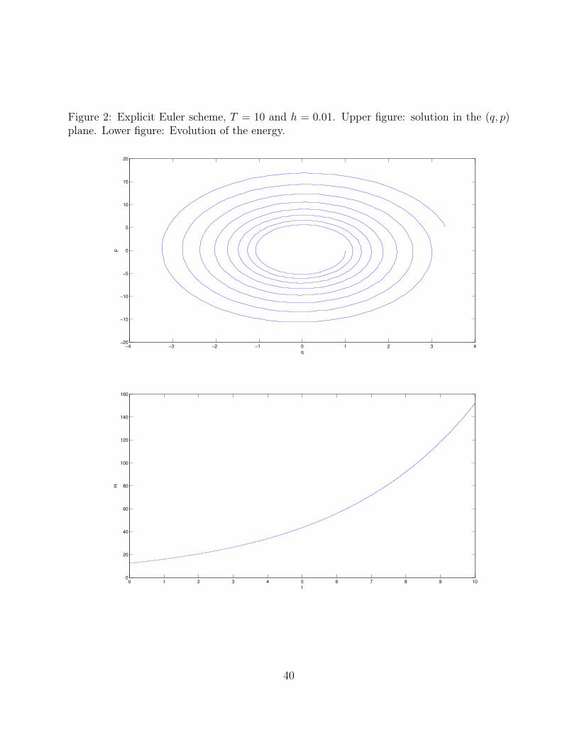
Figure 2: Explicit Euler scheme, T = 10 and h = 0.01. Upper figure: solution in the (q, p)plane. Lower figure: Evolution of the energy.

−4 −3 −2 −1 0 1 2 3 4−20

−15

−10

−5

0

5

10

15

20

q

p

0 1 2 3 4 5 6 7 8 9 100

20

40

60

80

100

120

140

160

t

H

40

Figure 3: Implicit Euler scheme, T = 10 and h = 0.01. Upper figure: solution in the (q, p)plane. Lower figure: Evolution of the energy.

−1 −0.8 −0.6 −0.4 −0.2 0 0.2 0.4 0.6 0.8 1−5

−4

−3

−2

−1

0

1

2

3

4

5

q

p

0 1 2 3 4 5 6 7 8 9 100

2

4

6

8

10

12

14

t

H

41

Figure 4: Euler schemes, T = 100 and h = 0.1. Upper figure: explicit scheme. Lower figure:implicit scheme.

−2 −1.5 −1 −0.5 0 0.5 1

x 1048

−1

−0.5

0

0.5

1

1.5x 10

49

q

p

−0.5 0 0.5 1−4

−3

−2

−1

0

1

2

q

p

42

Figure 5: Crank-Nicolson scheme. Upper figure: T = 10, h = 0.01. Lower figure: T = 100,h = 0.1.

−1 −0.8 −0.6 −0.4 −0.2 0 0.2 0.4 0.6 0.8 1−5

−4

−3

−2

−1

0

1

2

3

4

5

q

p

−1 −0.8 −0.6 −0.4 −0.2 0 0.2 0.4 0.6 0.8 1−5

−4

−3

−2

−1

0

1

2

3

4

5

q

p

43

Figure 6: Symplectic Euler scheme, T = 10, h = 0.01. Upper figure: solution in the (q, p)plane. Lower figure: Evolution of the energy.

−1 −0.8 −0.6 −0.4 −0.2 0 0.2 0.4 0.6 0.8 1−5

−4

−3

−2

−1

0

1

2

3

4

5

q

p

0 1 2 3 4 5 6 7 8 9 10

12.2

12.3

12.4

12.5

12.6

12.7

12.8

12.9

13

t

H

44

Figure 7: Symplectic Euler scheme, T = 100, h = 0.1. Upper figure: solution in the (q, p)plane. Lower figure: Evolution of the energy.

−1.5 −1 −0.5 0 0.5 1 1.5−6

−4

−2

0

2

4

6

q

p

0 10 20 30 40 50 60 70 80 90 10010

11

12

13

14

15

16

17

t

H

45

Figure 8: Störmer-Verlet scheme, T = 10, h = 0.01. Upper figure: solution in the (q, p)plane. Lower figure: Evolution of the energy.

−1 −0.8 −0.6 −0.4 −0.2 0 0.2 0.4 0.6 0.8 1−5

−4

−3

−2

−1

0

1

2

3

4

5

q

p

0 1 2 3 4 5 6 7 8 9 1012.492

12.493

12.494

12.495

12.496

12.497

12.498

12.499

12.5

t

H

46

Figure 9: Störmer-Verlet scheme, T = 100, h = 0.1. Upper figure: solution in the (q, p)plane. Lower figure: Evolution of the energy.

−1 −0.8 −0.6 −0.4 −0.2 0 0.2 0.4 0.6 0.8 1−5

−4

−3

−2

−1

0

1

2

3

4

5

q

p

0 10 20 30 40 50 60 70 80 90 10011.7

11.8

11.9

12

12.1

12.2

12.3

12.4

12.5

12.6

t

Q

47