introduction to optimization - john wiley & sons · introduction to optimization 1.1...
TRANSCRIPT
1
Introduction to Optimization
1.1 INTRODUCTION
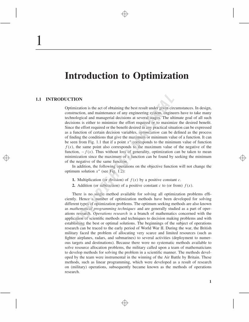
Optimization is the act of obtaining the best result under given circumstances. In design,construction, and maintenance of any engineering system, engineers have to take manytechnological and managerial decisions at several stages. The ultimate goal of all suchdecisions is either to minimize the effort required or to maximize the desired benefit.Since the effort required or the benefit desired in any practical situation can be expressedas a function of certain decision variables, optimization can be defined as the processof finding the conditions that give the maximum or minimum value of a function. It canbe seen from Fig. 1.1 that if a point x∗ corresponds to the minimum value of functionf (x), the same point also corresponds to the maximum value of the negative of thefunction, −f (x). Thus without loss of generality, optimization can be taken to meanminimization since the maximum of a function can be found by seeking the minimumof the negative of the same function.
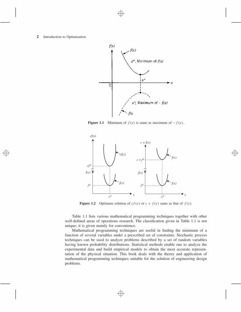
In addition, the following operations on the objective function will not change theoptimum solution x∗ (see Fig. 1.2):
1. Multiplication (or division) of f (x) by a positive constant c.2. Addition (or subtraction) of a positive constant c to (or from) f (x).
There is no single method available for solving all optimization problems effi-ciently. Hence a number of optimization methods have been developed for solvingdifferent types of optimization problems. The optimum seeking methods are also knownas mathematical programming techniques and are generally studied as a part of oper-ations research. Operations research is a branch of mathematics concerned with theapplication of scientific methods and techniques to decision making problems and withestablishing the best or optimal solutions. The beginnings of the subject of operationsresearch can be traced to the early period of World War II. During the war, the Britishmilitary faced the problem of allocating very scarce and limited resources (such asfighter airplanes, radars, and submarines) to several activities (deployment to numer-ous targets and destinations). Because there were no systematic methods available tosolve resource allocation problems, the military called upon a team of mathematiciansto develop methods for solving the problem in a scientific manner. The methods devel-oped by the team were instrumental in the winning of the Air Battle by Britain. Thesemethods, such as linear programming, which were developed as a result of researchon (military) operations, subsequently became known as the methods of operationsresearch.
1
COPYRIG
HTED M
ATERIAL
2 Introduction to Optimization
Figure 1.1 Minimum of f (x) is same as maximum of −f (x).
cf(x)
cf(x)
f(x)
f(x)
f(x)
f(x) f(x)
cf*
f* f*
x* xx*
x
c + f(x)
c + f*
Figure 1.2 Optimum solution of cf (x) or c + f (x) same as that of f (x).
Table 1.1 lists various mathematical programming techniques together with otherwell-defined areas of operations research. The classification given in Table 1.1 is notunique; it is given mainly for convenience.
Mathematical programming techniques are useful in finding the minimum of afunction of several variables under a prescribed set of constraints. Stochastic processtechniques can be used to analyze problems described by a set of random variableshaving known probability distributions. Statistical methods enable one to analyze theexperimental data and build empirical models to obtain the most accurate represen-tation of the physical situation. This book deals with the theory and application ofmathematical programming techniques suitable for the solution of engineering designproblems.

1.2 Historical Development 3
Table 1.1 Methods of Operations Research
Mathematical programming or Stochastic processoptimization techniques techniques Statistical methods
Calculus methods Statistical decision theory Regression analysisCalculus of variations Markov processes Cluster analysis, pattern
recognitionNonlinear programming Queueing theoryGeometric programming Renewal theory Design of experimentsQuadratic programming Simulation methods Discriminate analysis
(factor analysis)Linear programming Reliability theoryDynamic programmingInteger programmingStochastic programmingSeparable programmingMultiobjective programmingNetwork methods: CPM and PERTGame theory
Modern or nontraditional optimization techniques
Genetic algorithmsSimulated annealingAnt colony optimizationParticle swarm optimizationNeural networksFuzzy optimization
1.2 HISTORICAL DEVELOPMENT
The existence of optimization methods can be traced to the days of Newton, Lagrange,and Cauchy. The development of differential calculus methods of optimization waspossible because of the contributions of Newton and Leibnitz to calculus. The founda-tions of calculus of variations, which deals with the minimization of functionals, werelaid by Bernoulli, Euler, Lagrange, and Weirstrass. The method of optimization for con-strained problems, which involves the addition of unknown multipliers, became knownby the name of its inventor, Lagrange. Cauchy made the first application of the steep-est descent method to solve unconstrained minimization problems. Despite these earlycontributions, very little progress was made until the middle of the twentieth century,when high-speed digital computers made implementation of the optimization proce-dures possible and stimulated further research on new methods. Spectacular advancesfollowed, producing a massive literature on optimization techniques. This advance-ment also resulted in the emergence of several well-defined new areas in optimizationtheory.
It is interesting to note that the major developments in the area of numerical meth-ods of unconstrained optimization have been made in the United Kingdom only in the1960s. The development of the simplex method by Dantzig in 1947 for linear program-ming problems and the annunciation of the principle of optimality in 1957 by Bellmanfor dynamic programming problems paved the way for development of the methodsof constrained optimization. Work by Kuhn and Tucker in 1951 on the necessary and
4 Introduction to Optimization
sufficiency conditions for the optimal solution of programming problems laid the foun-dations for a great deal of later research in nonlinear programming. The contributionsof Zoutendijk and Rosen to nonlinear programming during the early 1960s have beensignificant. Although no single technique has been found to be universally applica-ble for nonlinear programming problems, work of Carroll and Fiacco and McCormickallowed many difficult problems to be solved by using the well-known techniques ofunconstrained optimization. Geometric programming was developed in the 1960s byDuffin, Zener, and Peterson. Gomory did pioneering work in integer programming,one of the most exciting and rapidly developing areas of optimization. The reason forthis is that most real-world applications fall under this category of problems. Dantzigand Charnes and Cooper developed stochastic programming techniques and solvedproblems by assuming design parameters to be independent and normally distributed.
The desire to optimize more than one objective or goal while satisfying the phys-ical limitations led to the development of multiobjective programming methods. Goalprogramming is a well-known technique for solving specific types of multiobjectiveoptimization problems. The goal programming was originally proposed for linear prob-lems by Charnes and Cooper in 1961. The foundations of game theory were laid byvon Neumann in 1928 and since then the technique has been applied to solve severalmathematical economics and military problems. Only during the last few years hasgame theory been applied to solve engineering design problems.
Modern Methods of Optimization. The modern optimization methods, also some-times called nontraditional optimization methods, have emerged as powerful and pop-ular methods for solving complex engineering optimization problems in recent years.These methods include genetic algorithms, simulated annealing, particle swarm opti-mization, ant colony optimization, neural network-based optimization, and fuzzy opti-mization. The genetic algorithms are computerized search and optimization algorithmsbased on the mechanics of natural genetics and natural selection. The genetic algorithmswere originally proposed by John Holland in 1975. The simulated annealing methodis based on the mechanics of the cooling process of molten metals through annealing.The method was originally developed by Kirkpatrick, Gelatt, and Vecchi.
The particle swarm optimization algorithm mimics the behavior of social organismssuch as a colony or swarm of insects (for example, ants, termites, bees, and wasps), aflock of birds, and a school of fish. The algorithm was originally proposed by Kennedyand Eberhart in 1995. The ant colony optimization is based on the cooperative behaviorof ant colonies, which are able to find the shortest path from their nest to a foodsource. The method was first developed by Marco Dorigo in 1992. The neural networkmethods are based on the immense computational power of the nervous system to solveperceptional problems in the presence of massive amount of sensory data through itsparallel processing capability. The method was originally used for optimization byHopfield and Tank in 1985. The fuzzy optimization methods were developed to solveoptimization problems involving design data, objective function, and constraints statedin imprecise form involving vague and linguistic descriptions. The fuzzy approachesfor single and multiobjective optimization in engineering design were first presentedby Rao in 1986.

1.3 Engineering Applications of Optimization 5
1.3 ENGINEERING APPLICATIONS OF OPTIMIZATION
Optimization, in its broadest sense, can be applied to solve any engineering problem.Some typical applications from different engineering disciplines indicate the wide scopeof the subject:
1. Design of aircraft and aerospace structures for minimum weight2. Finding the optimal trajectories of space vehicles3. Design of civil engineering structures such as frames, foundations, bridges,
towers, chimneys, and dams for minimum cost4. Minimum-weight design of structures for earthquake, wind, and other types of
random loading5. Design of water resources systems for maximum benefit6. Optimal plastic design of structures7. Optimum design of linkages, cams, gears, machine tools, and other mechanical
components8. Selection of machining conditions in metal-cutting processes for minimum pro-
duction cost9. Design of material handling equipment, such as conveyors, trucks, and cranes,
for minimum cost10. Design of pumps, turbines, and heat transfer equipment for maximum efficiency11. Optimum design of electrical machinery such as motors, generators, and trans-
formers12. Optimum design of electrical networks13. Shortest route taken by a salesperson visiting various cities during one tour14. Optimal production planning, controlling, and scheduling15. Analysis of statistical data and building empirical models from experimental
results to obtain the most accurate representation of the physical phenomenon16. Optimum design of chemical processing equipment and plants17. Design of optimum pipeline networks for process industries18. Selection of a site for an industry19. Planning of maintenance and replacement of equipment to reduce operating
costs20. Inventory control21. Allocation of resources or services among several activities to maximize the
benefit22. Controlling the waiting and idle times and queueing in production lines to reduce
the costs23. Planning the best strategy to obtain maximum profit in the presence of a com-
petitor24. Optimum design of control systems
6 Introduction to Optimization
1.4 STATEMENT OF AN OPTIMIZATION PROBLEM
An optimization or a mathematical programming problem can be stated as follows.
Find X =
⎧⎪⎪⎪⎨
⎪⎪⎪⎩
x1
x2...
xn
⎫⎪⎪⎪⎬
⎪⎪⎪⎭
which minimizes f (X)
subject to the constraints
gj (X) ≤ 0, j = 1, 2, . . . , m
lj (X) = 0, j = 1, 2, . . . , p(1.1)
where X is an n-dimensional vector called the design vector , f (X) is termed the objec-tive function , and gj (X) and lj (X) are known as inequality and equality constraints,respectively. The number of variables n and the number of constraints m and/or p
need not be related in any way. The problem stated in Eq. (1.1) is called a constrainedoptimization problem.† Some optimization problems do not involve any constraints andcan be stated as
Find X =
⎧⎪⎪⎪⎨
⎪⎪⎪⎩
x1
x2...
xn
⎫⎪⎪⎪⎬
⎪⎪⎪⎭
which minimizes f (X) (1.2)
Such problems are called unconstrained optimization problems .
1.4.1 Design Vector
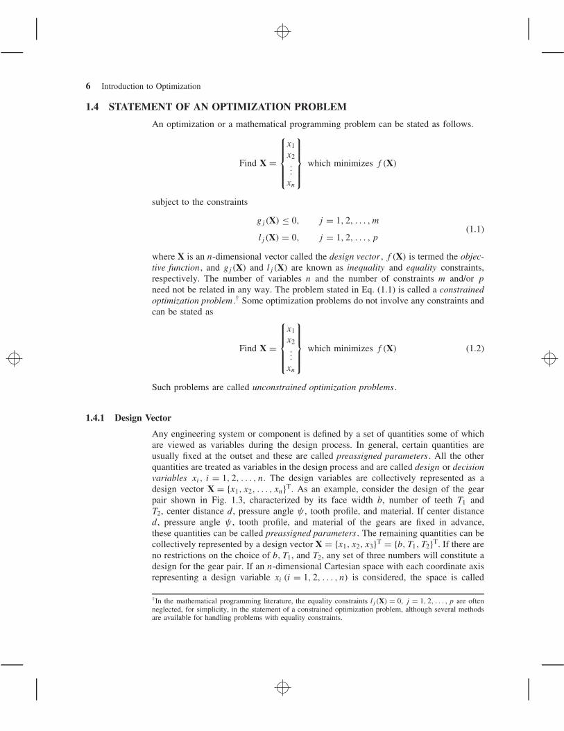
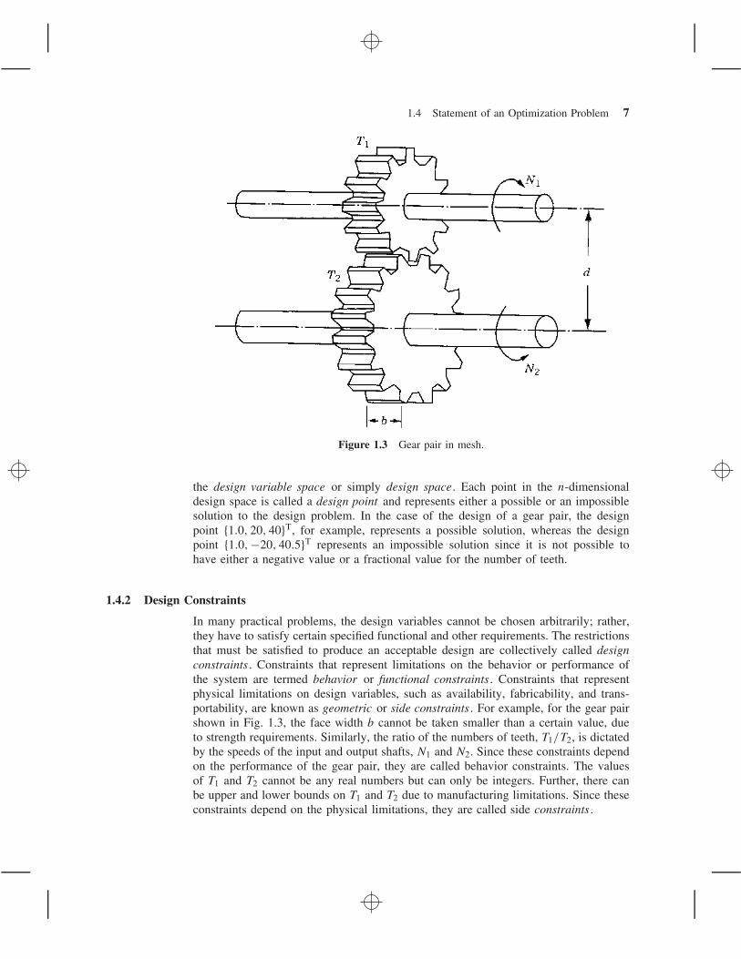
Any engineering system or component is defined by a set of quantities some of whichare viewed as variables during the design process. In general, certain quantities areusually fixed at the outset and these are called preassigned parameters . All the otherquantities are treated as variables in the design process and are called design or decisionvariables xi, i = 1, 2, . . . , n. The design variables are collectively represented as adesign vector X = {x1, x2, . . . , xn}T. As an example, consider the design of the gearpair shown in Fig. 1.3, characterized by its face width b, number of teeth T1 andT2, center distance d , pressure angle ψ , tooth profile, and material. If center distanced , pressure angle ψ , tooth profile, and material of the gears are fixed in advance,these quantities can be called preassigned parameters . The remaining quantities can becollectively represented by a design vector X = {x1, x2, x3}T = {b, T1, T2}T. If there areno restrictions on the choice of b, T1, and T2, any set of three numbers will constitute adesign for the gear pair. If an n-dimensional Cartesian space with each coordinate axisrepresenting a design variable xi (i = 1, 2, . . . , n) is considered, the space is called
†In the mathematical programming literature, the equality constraints lj (X) = 0, j = 1, 2, . . . , p are oftenneglected, for simplicity, in the statement of a constrained optimization problem, although several methodsare available for handling problems with equality constraints.
1.4 Statement of an Optimization Problem 7
Figure 1.3 Gear pair in mesh.
the design variable space or simply design space. Each point in the n-dimensionaldesign space is called a design point and represents either a possible or an impossiblesolution to the design problem. In the case of the design of a gear pair, the designpoint {1.0, 20, 40}T, for example, represents a possible solution, whereas the designpoint {1.0, −20, 40.5}T represents an impossible solution since it is not possible tohave either a negative value or a fractional value for the number of teeth.
1.4.2 Design Constraints
In many practical problems, the design variables cannot be chosen arbitrarily; rather,they have to satisfy certain specified functional and other requirements. The restrictionsthat must be satisfied to produce an acceptable design are collectively called designconstraints . Constraints that represent limitations on the behavior or performance ofthe system are termed behavior or functional constraints . Constraints that representphysical limitations on design variables, such as availability, fabricability, and trans-portability, are known as geometric or side constraints . For example, for the gear pairshown in Fig. 1.3, the face width b cannot be taken smaller than a certain value, dueto strength requirements. Similarly, the ratio of the numbers of teeth, T1/T2, is dictatedby the speeds of the input and output shafts, N1 and N2. Since these constraints dependon the performance of the gear pair, they are called behavior constraints. The valuesof T1 and T2 cannot be any real numbers but can only be integers. Further, there canbe upper and lower bounds on T1 and T2 due to manufacturing limitations. Since theseconstraints depend on the physical limitations, they are called side constraints .

8 Introduction to Optimization
1.4.3 Constraint Surface
For illustration, consider an optimization problem with only inequality constraintsgj (X) ≤ 0. The set of values of X that satisfy the equation gj (X) = 0 forms a hyper-surface in the design space and is called a constraint surface. Note that this is an(n − 1)-dimensional subspace, where n is the number of design variables. The constraintsurface divides the design space into two regions: one in which gj (X) < 0 and the otherin which gj (X) > 0. Thus the points lying on the hypersurface will satisfy the constraintgj (X) critically, whereas the points lying in the region where gj (X) > 0 are infeasibleor unacceptable, and the points lying in the region where gj (X) < 0 are feasible oracceptable. The collection of all the constraint surfaces gj (X) = 0, j = 1, 2, . . . ,m,which separates the acceptable region is called the composite constraint surface.
Figure 1.4 shows a hypothetical two-dimensional design space where the infeasibleregion is indicated by hatched lines. A design point that lies on one or more than oneconstraint surface is called a bound point , and the associated constraint is called anactive constraint . Design points that do not lie on any constraint surface are known asfree points . Depending on whether a particular design point belongs to the acceptableor unacceptable region, it can be identified as one of the following four types:
1. Free and acceptable point2. Free and unacceptable point3. Bound and acceptable point4. Bound and unacceptable point
All four types of points are shown in Fig. 1.4.
Figure 1.4 Constraint surfaces in a hypothetical two-dimensional design space.

1.4 Statement of an Optimization Problem 9
1.4.4 Objective Function
The conventional design procedures aim at finding an acceptable or adequate designthat merely satisfies the functional and other requirements of the problem. In general,there will be more than one acceptable design, and the purpose of optimization isto choose the best one of the many acceptable designs available. Thus a criterionhas to be chosen for comparing the different alternative acceptable designs and forselecting the best one. The criterion with respect to which the design is optimized,when expressed as a function of the design variables, is known as the criterion or meritor objective function . The choice of objective function is governed by the nature ofproblem. The objective function for minimization is generally taken as weight in aircraftand aerospace structural design problems. In civil engineering structural designs, theobjective is usually taken as the minimization of cost. The maximization of mechanicalefficiency is the obvious choice of an objective in mechanical engineering systemsdesign. Thus the choice of the objective function appears to be straightforward in mostdesign problems. However, there may be cases where the optimization with respectto a particular criterion may lead to results that may not be satisfactory with respectto another criterion. For example, in mechanical design, a gearbox transmitting themaximum power may not have the minimum weight. Similarly, in structural design,the minimum weight design may not correspond to minimum stress design, and theminimum stress design, again, may not correspond to maximum frequency design. Thusthe selection of the objective function can be one of the most important decisions inthe whole optimum design process.
In some situations, there may be more than one criterion to be satisfied simul-taneously. For example, a gear pair may have to be designed for minimum weightand maximum efficiency while transmitting a specified horsepower. An optimizationproblem involving multiple objective functions is known as a multiobjective program-ming problem . With multiple objectives there arises a possibility of conflict, and onesimple way to handle the problem is to construct an overall objective function as alinear combination of the conflicting multiple objective functions. Thus if f1(X) andf2(X) denote two objective functions, construct a new (overall) objective function foroptimization as
f (X) = α1f1(X) + α2f2(X) (1.3)
where α1 and α2 are constants whose values indicate the relative importance of oneobjective function relative to the other.
1.4.5 Objective Function Surfaces
The locus of all points satisfying f (X) = C = constant forms a hypersurface in thedesign space, and each value of C corresponds to a different member of a family ofsurfaces. These surfaces, called objective function surfaces , are shown in a hypotheticaltwo-dimensional design space in Fig. 1.5.
Once the objective function surfaces are drawn along with the constraint surfaces,the optimum point can be determined without much difficulty. But the main problemis that as the number of design variables exceeds two or three, the constraint andobjective function surfaces become complex even for visualization and the problem

10 Introduction to Optimization
Figure 1.5 Contours of the objective function.
has to be solved purely as a mathematical problem. The following example illustratesthe graphical optimization procedure.
Example 1.1 Design a uniform column of tubular section, with hinge joints at bothends, (Fig. 1.6) to carry a compressive load P = 2500 kgf for minimum cost. Thecolumn is made up of a material that has a yield stress (σy) of 500 kgf/cm2, modulusof elasticity (E) of 0.85 × 10⁶ kgf/cm2, and weight density (ρ) of 0.0025 kgf/cm3.The length of the column is 250 cm. The stress induced in the column should be lessthan the buckling stress as well as the yield stress. The mean diameter of the columnis restricted to lie between 2 and 14 cm, and columns with thicknesses outside therange 0.2 to 0.8 cm are not available in the market. The cost of the column includesmaterial and construction costs and can be taken as 5W + 2d , where W is the weightin kilograms force and d is the mean diameter of the column in centimeters.
SOLUTION The design variables are the mean diameter (d) and tube thickness (t):
X ={x1
x2
}
={d
t
}
(E1)
The objective function to be minimized is given by
f (X) = 5W + 2d = 5ρlπ dt + 2d = 9.82x1x2 + 2x1 (E2)

1.4 Statement of an Optimization Problem 11
i
Figure 1.6 Tubular column under compression.
The behavior constraints can be expressed as
stress induced ≤ yield stress
stress induced ≤ buckling stress
The induced stress is given by
induced stress = σi = P
π dt= 2500
πx1x2(E3)
The buckling stress for a pin-connected column is given by
buckling stress = σb = Euler buckling load
cross-sectional area= π2EI
l2
1
π dt(E4)
where
I = second moment of area of the cross section of the column
= π
64(d4
o − d4i )
= π
64(d2
o + d2i )(do + di)(do − di) = π
64[(d + t)2 + (d − t)2]
× [(d + t) + (d − t)][(d + t) − (d − t)]
= π
8dt (d2 + t2) = π
8x1x2(x
21 + x2
2 ) (E5)

12 Introduction to Optimization
Thus the behavior constraints can be restated as
g1(X) = 2500
πx1x2− 500 ≤ 0 (E6)
g2(X) = 2500
πx1x2− π2(0.85 × 10⁶)(x2
1 + x22 )
8(250)2≤ 0 (E7)
The side constraints are given by
2 ≤ d ≤ 14
0.2 ≤ t ≤ 0.8
which can be expressed in standard form as
g3(X) = −x1 + 2.0 ≤ 0 (E8)
g4(X) = x1 − 14.0 ≤ 0 (E9)
g5(X) = −x2 + 0.2 ≤ 0 (E10)
g6(X) = x2 − 0.8 ≤ 0 (E11)
Since there are only two design variables, the problem can be solved graphically asshown below.
First, the constraint surfaces are to be plotted in a two-dimensional design spacewhere the two axes represent the two design variables x1 and x2. To plot the firstconstraint surface, we have
g1(X) = 2500
πx1x2− 500 ≤ 0
that is,x1x2 ≥ 1.593
Thus the curve x1x2 = 1.593 represents the constraint surface g1(X) = 0. This curvecan be plotted by finding several points on the curve. The points on the curve can befound by giving a series of values to x1 and finding the corresponding values of x2
that satisfy the relation x1x2 = 1.593:
x1 2.0 4.0 6.0 8.0 10.0 12.0 14.0
x2 0.7965 0.3983 0.2655 0.1990 0.1593 0.1328 0.1140
These points are plotted and a curve P1Q1 passing through all these points is drawn asshown in Fig. 1.7, and the infeasible region, represented by g1(X) > 0 or x1x2 < 1.593,is shown by hatched lines.† Similarly, the second constraint g2(X) ≤ 0 can be expressedas x1x2(x
21 + x2
2) ≥ 47.3 and the points lying on the constraint surface g2(X) = 0 canbe obtained as follows for x1x2(x
21 + x2
2) = 47.3:
†The infeasible region can be identified by testing whether the origin lies in the feasible or infeasibleregion.

1.4 Statement of an Optimization Problem 13
Figure 1.7 Graphical optimization of Example 1.1.
x1 2 4 6 8 10 12 14
x2 2.41 0.716 0.219 0.0926 0.0473 0.0274 0.0172
These points are plotted as curve P2Q2, the feasible region is identified, and the infea-sible region is shown by hatched lines as in Fig. 1.7. The plotting of side constraintsis very simple since they represent straight lines. After plotting all the six constraints,the feasible region can be seen to be given by the bounded area ABCDEA.

14 Introduction to Optimization
Next, the contours of the objective function are to be plotted before finding theoptimum point. For this, we plot the curves given by
f (X) = 9.82x1x2 + 2x1 = c = constant
for a series of values of c. By giving different values to c, the contours of f can beplotted with the help of the following points.
For 9.82x1x2 + 2x1 = 50.0:
x2 0.1 0.2 0.3 0.4 0.5 0.6 0.7 0.8
x1 16.77 12.62 10.10 8.44 7.24 6.33 5.64 5.07
For 9.82x1x2 + 2x1 = 40.0:
x2 0.1 0.2 0.3 0.4 0.5 0.6 0.7 0.8
x1 13.40 10.10 8.08 6.75 5.79 5.06 4.51 4.05
For 9.82x1x2 + 2x1 = 31.58 (passing through the corner point C):
x2 0.1 0.2 0.3 0.4 0.5 0.6 0.7 0.8
x1 10.57 7.96 6.38 5.33 4.57 4.00 3.56 3.20
For 9.82x1x2 + 2x1 = 26.53 (passing through the corner point B):
x2 0.1 0.2 0.3 0.4 0.5 0.6 0.7 0.8
x1 8.88 6.69 5.36 4.48 3.84 3.36 2.99 2.69
For 9.82x1x2 + 2x1 = 20.0:
x2 0.1 0.2 0.3 0.4 0.5 0.6 0.7 0.8
x1 6.70 5.05 4.04 3.38 2.90 2.53 2.26 2.02
These contours are shown in Fig. 1.7 and it can be seen that the objective functioncannot be reduced below a value of 26.53 (corresponding to point B) without violatingsome of the constraints. Thus the optimum solution is given by point B with d∗ =x∗
1 = 5.44 cm and t∗ = x∗2 = 0.293 cm with fmin = 26.53.
1.5 CLASSIFICATION OF OPTIMIZATION PROBLEMS
Optimization problems can be classified in several ways, as described below.
1.5.1 Classification Based on the Existence of Constraints
As indicated earlier, any optimization problem can be classified as constrained or uncon-strained, depending on whether constraints exist in the problem.

1.5 Classification of Optimization Problems 15
1.5.2 Classification Based on the Nature of the Design Variables
Based on the nature of design variables encountered, optimization problems can beclassified into two broad categories. In the first category, the problem is to find valuesto a set of design parameters that make some prescribed function of these parametersminimum subject to certain constraints. For example, the problem of minimum-weightdesign of a prismatic beam shown in Fig. 1.8a subject to a limitation on the maximumdeflection can be stated as follows:
Find X ={b
d
}
which minimizes
f (X) = ρlbd
(1.4)
subject to the constraints
δtip(X) ≤ δmax
b ≥ 0
d ≥ 0
where ρ is the density and δtip is the tip deflection of the beam. Such problems arecalled parameter or static optimization problems . In the second category of problems,the objective is to find a set of design parameters, which are all continuous functionsof some other parameter, that minimizes an objective function subject to a set ofconstraints. If the cross-sectional dimensions of the rectangular beam are allowed tovary along its length as shown in Fig. 1.8b, the optimization problem can be stated as
Find X(t) ={b(t)
d(t)
}
which minimizes
f [X(t)] = ρ
∫ l
0b(t) d(t) dt (1.5)
subject to the constraints
δtip[X(t)] ≤ δmax, 0 ≤ t ≤ l
b(t) ≥ 0, 0 ≤ t ≤ l
d(t) ≥ 0, 0 ≤ t ≤ l
Figure 1.8 Cantilever beam under concentrated load.

16 Introduction to Optimization
Here the design variables are functions of the length parameter t . This type of problem,where each design variable is a function of one or more parameters, is known as atrajectory or dynamic optimization problem [1.55].
1.5.3 Classification Based on the Physical Structure of the Problem
Depending on the physical structure of the problem, optimization problems can beclassified as optimal control and nonoptimal control problems.
Optimal Control Problem. An optimal control (OC) problem is a mathematical pro-gramming problem involving a number of stages, where each stage evolves from thepreceding stage in a prescribed manner. It is usually described by two types of vari-ables: the control (design) and the state variables. The control variables define thesystem and govern the evolution of the system from one stage to the next, and the statevariables describe the behavior or status of the system in any stage. The problem isto find a set of control or design variables such that the total objective function (alsoknown as the performance index , PI) over all the stages is minimized subject to aset of constraints on the control and state variables. An OC problem can be stated asfollows [1.55]:
Find X which minimizes f (X) =l∑
i=1
fi(xi , yi) (1.6)
subject to the constraints
qi(xi , yi) + yi = yi+1, i = 1, 2, . . . , l
gj (xj ) ≤ 0, j = 1, 2, . . . , l
hk(yk) ≤ 0, k = 1, 2, . . . , l
where xi is the ith control variable, yi the ith state variable, and fi the contributionof the ith stage to the total objective function; gj , hk, and qi are functions of xj , yk,and xi and yi , respectively, and l is the total number of stages. The control and statevariables xi and yi can be vectors in some cases. The following example serves toillustrate the nature of an optimal control problem.
Example 1.2 A rocket is designed to travel a distance of 12s in a vertically upwarddirection [1.39]. The thrust of the rocket can be changed only at the discrete pointslocated at distances of 0, s, 2s, 3s, . . . , 12s. If the maximum thrust that can be devel-oped at point i either in the positive or negative direction is restricted to a value ofFi , formulate the problem of minimizing the total time of travel under the followingassumptions:
1. The rocket travels against the gravitational force.2. The mass of the rocket reduces in proportion to the distance traveled.3. The air resistance is proportional to the velocity of the rocket.

1.5 Classification of Optimization Problems 17
Figure 1.9 Control points in the path of the rocket.
SOLUTION Let points (or control points) on the path at which the thrusts of therocket are changed be numbered as 1, 2, 3, . . . , 13 (Fig. 1.9). Denoting xi as the thrust,vi the velocity, ai the acceleration, and mi the mass of the rocket at point i, Newton’ssecond law of motion can be applied as
net force on the rocket = mass × acceleration
This can be written as
thrust − gravitational force − air resistance = mass × acceleration

18 Introduction to Optimization
or
xi − mig − k1vi = miai (E1)
where the mass mi can be expressed as
mi = mi−1 − k2s (E2)
and k1 and k2 are constants. Equation (E1) can be used to express the acceleration, ai ,as
ai = xi
mi
− g − k1vi
mi
(E3)
If ti denotes the time taken by the rocket to travel from point i to point i + 1, thedistance traveled between the points i and i + 1 can be expressed as
s = viti + 12ait
2i
or
1
2t2i
(xi
mi
− g − k1vi
mi
)
+ tivi − s = 0 (E4)
from which ti can be determined as
ti =−vi ±
√
v2i + 2s
(xi
mi
− g − k1vi
mi
)
xi
mi
− g − k1vi
mi
(E5)
Of the two values given by Eq. (E5), the positive value has to be chosen for ti . Thevelocity of the rocket at point i + 1, vi+1, can be expressed in terms of vi as (byassuming the acceleration between points i and i + 1 to be constant for simplicity)
vi+1 = vi + aiti (E6)
The substitution of Eqs. (E3) and (E5) into Eq. (E6) leads to
vi+1 =√
v2i + 2s
(xi
mi
− g − k1vi
mi
)
(E7)
From an analysis of the problem, the control variables can be identified as the thrusts,xi , and the state variables as the velocities, vi . Since the rocket starts at point 1 andstops at point 13,
v1 = v13 = 0 (E8)

1.5 Classification of Optimization Problems 19
Thus the problem can be stated as an OC problem as
Find X =
⎧⎪⎪⎪⎨
⎪⎪⎪⎩
x1
x2...
x12
⎫⎪⎪⎪⎬
⎪⎪⎪⎭
which minimizes
f (X) =12∑
i=1
ti =12∑
i=1
⎧⎪⎪⎪⎪⎨
⎪⎪⎪⎪⎩
−vi +√
v2i + 2s
(xi
mi
− g − k1vi
mi
)
xi
mi
− g − k1vi
mi
⎫⎪⎪⎪⎪⎬
⎪⎪⎪⎪⎭
subject to
mi+1 = mi − k2s, i = 1, 2, . . . , 12
vi+1 =√
v2i + 2s
(xi
mi
− g − k1vi
mi
)
, i = 1, 2, . . . , 12
|xi | ≤ Fi, i = 1, 2, . . . , 12
v1 = v13 = 0
1.5.4 Classification Based on the Nature of the Equations Involved
Another important classification of optimization problems is based on the nature ofexpressions for the objective function and the constraints. According to this classi-fication, optimization problems can be classified as linear, nonlinear, geometric, andquadratic programming problems. This classification is extremely useful from the com-putational point of view since there are many special methods available for the efficientsolution of a particular class of problems. Thus the first task of a designer would beto investigate the class of problem encountered. This will, in many cases, dictate thetypes of solution procedures to be adopted in solving the problem.
Nonlinear Programming Problem. If any of the functions among the objective andconstraint functions in Eq. (1.1) is nonlinear, the problem is called a nonlinear pro-gramming (NLP) problem . This is the most general programming problem and all otherproblems can be considered as special cases of the NLP problem.
Example 1.3 The step-cone pulley shown in Fig. 1.10 is to be designed for trans-mitting a power of at least 0.75 hp. The speed of the input shaft is 350 rpm and theoutput speed requirements are 750, 450, 250, and 150 rpm for a fixed center distanceof a between the input and output shafts. The tension on the tight side of the belt is tobe kept more than twice that on the slack side. The thickness of the belt is t and thecoefficient of friction between the belt and the pulleys is μ. The stress induced in thebelt due to tension on the tight side is s. Formulate the problem of finding the widthand diameters of the steps for minimum weight.

20 Introduction to Optimization
Figure 1.10 Step-cone pulley.
SOLUTION The design vector can be taken as
X =
⎧⎪⎪⎪⎪⎪⎨
⎪⎪⎪⎪⎪⎩
d1
d2
d3
d4
w
⎫⎪⎪⎪⎪⎪⎬
⎪⎪⎪⎪⎪⎭
where di is the diameter of the ith step on the output pulley and w is the width of thebelt and the steps. The objective function is the weight of the step-cone pulley system:
f (X) = ρwπ
4(d2
1 + d22 + d2
3 + d24 + d ′ 2
1 + d ′ 22 + d ′ 2
3 + d ′ 24 )
= ρwπ
4
{
d21
[
1 +(
750
350
)2]
+ d22
[
1 +(
450
350
)2]
+ d23
[
1 +(
250
350
)2]
+ d24
[
1 +(
150
350
)2]}
(E1)
where ρ is the density of the pulleys and d ′i is the diameter of the ith step on the input
pulley.
1.5 Classification of Optimization Problems 21
To have the belt equally tight on each pair of opposite steps, the total length of thebelt must be kept constant for all the output speeds. This can be ensured by satisfyingthe following equality constraints:
C1 − C2 = 0 (E2)
C1 − C3 = 0 (E3)
C1 − C4 = 0 (E4)
where Ci denotes length of the belt needed to obtain output speed Ni (i = 1, 2, 3, 4)and is given by [1.116, 1.117]:
Ci � πdi
2
(
1 + Ni
N
)
+
(Ni
N− 1
)2
d2i
4a+ 2a
where N is the speed of the input shaft and a is the center distance between the shafts.The ratio of tensions in the belt can be expressed as [1.116, 1.117]
T i1
T i2
= eμθi
where T i1 and T i
2 are the tensions on the tight and slack sides of the ith step, μ thecoefficient of friction, and θi the angle of lap of the belt over the ith pulley step. Theangle of lap is given by
θi = π − 2 sin−1[
(Ni
N− 1
)
di
2a
]
and hence the constraint on the ratio of tensions becomes
exp
{
μ
[
π − 2 sin−1{(
Ni
N− 1
)di
2a
}]}
≥ 2, i = 1, 2, 3, 4 (E5)
The limitation on the maximum tension can be expressed as
T i1 = stw, i = 1, 2, 3, 4 (E6)
where s is the maximum allowable stress in the belt and t is the thickness of the belt.The constraint on the power transmitted can be stated as (using lbf for force and ft forlinear dimensions)
(T i1 − T i
2 )πd ′i (350)
33,000≥ 0.75
which can be rewritten, using T i1 = stw from Eq. (E6), as
stw
(
1 − exp
[
−μ
(
π − 2 sin−1{(
Ni
N− 1
)di
2a
})])
πd ′i
×(
350
33,000
)
≥ 0.75, i = 1, 2, 3, 4 (E7)

22 Introduction to Optimization
Finally, the lower bounds on the design variables can be taken as
w ≥ 0 (E8)
di ≥ 0, i = 1, 2, 3, 4 (E9)
As the objective function, (E1), and most of the constraints, (E2) to (E9), are nonlinearfunctions of the design variables d1, d2, d3, d4, and w, this problem is a nonlinearprogramming problem.
Geometric Programming Problem.
Definition A function h(X) is called a posynomial if h can be expressed as the sumof power terms each of the form
cixai11 xai2
2 · · · xainn
where ci and aij are constants with ci > 0 and xj > 0. Thus a posynomial with N termscan be expressed as
h(X) = c1xa111 xa12
2 · · · xa1nn + · · · + cNxaN1
1 xaN22 · · · xaNn
n (1.7)
A geometric programming (GMP) problem is one in which the objective functionand constraints are expressed as posynomials in X. Thus GMP problem can be posedas follows [1.59]:
Find X which minimizes
f (X) =N0∑
i=1
ci
⎛
⎝n∏
j=1
xpij
j
⎞
⎠ , ci > 0, xj > 0 (1.8)
subject to
gk(X) =Nk∑
i=1
aik
⎛
⎝n∏
j=1
xqijk
j
⎞
⎠ > 0, aik > 0, xj > 0, k = 1, 2, . . . , m
where N0 and Nk denote the number of posynomial terms in the objective and kthconstraint function, respectively.
Example 1.4 Four identical helical springs are used to support a milling machineweighing 5000 lb. Formulate the problem of finding the wire diameter (d), coil diameter(D), and the number of turns (N ) of each spring (Fig. 1.11) for minimum weight bylimiting the deflection to 0.1 in. and the shear stress to 10,000 psi in the spring. Inaddition, the natural frequency of vibration of the spring is to be greater than 100 Hz.The stiffness of the spring (k), the shear stress in the spring (τ ), and the naturalfrequency of vibration of the spring (fn) are given by
k = d4G
8D3N
τ = Ks
8FD
πd3
fn = 1
2
√kg
w= 1
2
√d4G
8D3N
g
ρ(πd2/4)πDN=
√Gg d
2√
2ρπD2N

1.5 Classification of Optimization Problems 23
Figure 1.11 Helical spring.
where G is the shear modulus, F the compressive load on the spring, w the weight ofthe spring, ρ the weight density of the spring, and Ks the shear stress correction factor.Assume that the material is spring steel with G = 12 × 106 psi and ρ = 0.3 lb/in3, andthe shear stress correction factor is Ks ≈ 1.05.
SOLUTION The design vector is given by
X =⎧⎨
⎩
x1
x2
x3
⎫⎬
⎭=
⎧⎨
⎩
d
D
N
⎫⎬
⎭
and the objective function by
f (X) = weight = πd2
4πDNρ (E1)
The constraints can be expressed as
deflection = F
k= 8FD3N
d4G≤ 0.1
that is,
g1(X) = d4G
80FD3N> 1 (E2)
shear stress = Ks
8FD
πd3≤ 10,000

24 Introduction to Optimization
that is,
g2(X) = 1250πd3
KsFD> 1 (E3)
natural frequency =√
Gg
2√
2ρπ
d
D2N≥ 100
that is,
g3(X) =√
Gg d
200√
2ρπD2N> 1 (E4)
Since the equality sign is not included (along with the inequality symbol, >) in theconstraints of Eqs. (E2) to (E4), the design variables are to be restricted to positivevalues as
d > 0, D > 0, N > 0 (E5)
By substituting the known data, F = weight of the milling machine/4 = 1250 lb, ρ =0.3 lb/in3, G = 12 × 106 psi, and Ks = 1.05, Eqs. (E1) to (E4) become
f (X) = 14π2(0.3)d2DN = 0.7402x2
1x2x3 (E6)
g1(X) = d4(12 × 106)
80(1250)D3N= 120x4
1x−32 x−1
3 > 1 (E7)
g2(X) = 1250πd3
1.05(1250)D= 2.992x3
1x−12 > 1 (E8)
g3(X) =√
Gg d
200√
2ρπD2N= 139.8388x1x
−22 x−1
3 > 1 (E9)
It can be seen that the objective function, f (X), and the constraint functions, g1(X) tog3(X), are posynomials and hence the problem is a GMP problem.
Quadratic Programming Problem. A quadratic programming problem is a nonlinearprogramming problem with a quadratic objective function and linear constraints. It isusually formulated as follows:
F(X) = c +n∑
i=1
qixi +n∑
i=1
n∑
j=1
Qijxixj (1.9)
subject ton∑
i=1
aij xi = bj , j = 1, 2, . . . , m
xi ≥ 0, i = 1, 2, . . . , n
where c, qi, Qij , aij , and bj are constants.

1.5 Classification of Optimization Problems 25
Example 1.5 A manufacturing firm produces two products, A and B, using two limitedresources. The maximum amounts of resources 1 and 2 available per day are 1000 and250 units, respectively. The production of 1 unit of product A requires 1 unit of resource1 and 0.2 unit of resource 2, and the production of 1 unit of product B requires 0.5unit of resource 1 and 0.5 unit of resource 2. The unit costs of resources 1 and 2 aregiven by the relations (0.375 − 0.00005u1) and (0.75 − 0.0001u2), respectively, whereui denotes the number of units of resource i used (i = 1, 2). The selling prices per unitof products A and B,pA and pB , are given by
pA = 2.00 − 0.0005xA − 0.00015xB
pB = 3.50 − 0.0002xA − 0.0015xB
where xA and xB indicate, respectively, the number of units of products A and B sold.Formulate the problem of maximizing the profit assuming that the firm can sell all theunits it manufactures.
SOLUTION Let the design variables be the number of units of products A and B
manufactured per day:
X ={xA
xB
}
The requirement of resource 1 per day is (xA + 0.5xB) and that of resource 2 is(0.2xA + 0.5xB) and the constraints on the resources are
xA + 0.5xB ≤ 1000 (E1)
0.2xA + 0.5xB ≤ 250 (E2)
The lower bounds on the design variables can be taken as
xA ≥ 0 (E3)
xB ≥ 0 (E4)
The total cost of resources 1 and 2 per day is
(xA + 0.5xB)[0.375 − 0.00005(xA + 0.5xB)]
+ (0.2xA + 0.5xB)[0.750 − 0.0001(0.2xA + 0.5xB)]
and the return per day from the sale of products A and B is
xA(2.00 − 0.0005xA − 0.00015xB) + xB(3.50 − 0.0002xA − 0.0015xB)
The total profit is given by the total return minus the total cost. Since the objectivefunction to be minimized is the negative of the profit per day, f (X) is given by
f (X) = (xA + 0.5xB)[0.375 − 0.00005(xA + 0.5xB)]
+ (0.2xA + 0.5xB)[0.750 − 0.0001(0.2xA + 0.5xB)]
− xA(2.00 − 0.0005xA − 0.00015xB)
− xB(3.50 − 0.0002xA − 0.0015xB) (E5)

26 Introduction to Optimization
As the objective function [Eq. (E5)] is a quadratic and the constraints [Eqs. (E1) to(E4)] are linear, the problem is a quadratic programming problem.
Linear Programming Problem. If the objective function and all the constraints inEq. (1.1) are linear functions of the design variables, the mathematical programmingproblem is called a linear programming (LP) problem . A linear programming problemis often stated in the following standard form:
Find X =
⎧⎪⎪⎪⎨
⎪⎪⎪⎩
x1
x2...
xn
⎫⎪⎪⎪⎬
⎪⎪⎪⎭
which minimizes f (X) =n∑
i=1
cixi
subject to the constraints (1.10)
n∑
i=1
aij xi = bj , j = 1, 2, . . . , m
xi ≥ 0, i = 1, 2, . . . , n
where ci, aij , and bj are constants.
Example 1.6 A scaffolding system consists of three beams and six ropes as shownin Fig. 1.12. Each of the top ropes A and B can carry a load of W1, each of themiddle ropes C and D can carry a load of W2, and each of the bottom ropes E andF can carry a load of W3. If the loads acting on beams 1, 2, and 3 are x1, x2, and x3,respectively, as shown in Fig. 1.12, formulate the problem of finding the maximum
Figure 1.12 Scaffolding system with three beams.

1.5 Classification of Optimization Problems 27
load (x1 + x2 + x3) that can be supported by the system. Assume that the weights ofthe beams 1, 2, and 3 are w1, w2, and w3, respectively, and the weights of the ropesare negligible.
SOLUTION Assuming that the weights of the beams act through their respectivemiddle points, the equations of equilibrium for vertical forces and moments for eachof the three beams can be written as
For beam 3:
TE + TF = x3 + w3
x3(3l) + w3(2l) − TF (4l) = 0
For beam 2:
TC + TD − TE = x2 + w2
x2(l) + w2(l) + TE(l) − TD(2l) = 0
For beam 1:
TA + TB − TC − TD − TF = x1 + w1
x1(3l) + w1(92 l) − TB(9l) + TC(2l) + TD(4l) + TF (7l) = 0
where Ti denotes the tension in rope i. The solution of these equations gives
TF = 34x3 + 1
2w3
TE = 14x3 + 1
2w3
TD = 12x2 + 1
8x3 + 12w2 + 1
4w3
TC = 12x2 + 1
8x3 + 12w2 + 1
4w3
TB = 13x1 + 1
3x2 + 23x3 + 1
2w1 + 13w2 + 5
9w3
TA = 23x1 + 2
3x2 + 13x3 + 1
2w1 + 23w2 + 4
9w3
The optimization problem can be formulated by choosing the design vector as
X =⎧⎨
⎩
x1
x2
x3
⎫⎬
⎭
Since the objective is to maximize the total load
f (X) = −(x1 + x2 + x3) (E1)
The constraints on the forces in the ropes can be stated as
TA ≤ W1 (E2)
TB ≤ W1 (E3)
TC ≤ W2 (E4)

28 Introduction to Optimization
TD ≤ W2 (E5)
TE ≤ W3 (E6)
TF ≤ W3 (E7)
Finally, the nonnegativity requirement of the design variables can be expressed as
x1 ≥ 0
x2 ≥ 0
x3 ≥ 0 (E8)
Since all the equations of the problem (E1) to (E8), are linear functions of x1, x2, andx3, the problem is a linear programming problem.
1.5.5 Classification Based on the Permissible Values of the Design Variables
Depending on the values permitted for the design variables, optimization problems canbe classified as integer and real-valued programming problems.
Integer Programming Problem. If some or all of the design variables x1, x2, . . . , xn
of an optimization problem are restricted to take on only integer (or discrete) values,the problem is called an integer programming problem . On the other hand, if all thedesign variables are permitted to take any real value, the optimization problem iscalled a real-valued programming problem . According to this definition, the problemsconsidered in Examples 1.1 to 1.6 are real-valued programming problems.
Example 1.7 A cargo load is to be prepared from five types of articles. The weightwi , volume vi , and monetary value ci of different articles are given below.
Article type wi vi ci
1 4 9 52 8 7 63 2 4 34 5 3 25 3 8 8
Find the number of articles xi selected from the ith type (i = 1, 2, 3, 4, 5), so that thetotal monetary value of the cargo load is a maximum. The total weight and volume ofthe cargo cannot exceed the limits of 2000 and 2500 units, respectively.
SOLUTION Let xi be the number of articles of type i (i = 1 to 5) selected. Sinceit is not possible to load a fraction of an article, the variables xi can take only integervalues.
The objective function to be maximized is given by
f (X) = 5x1 + 6x2 + 3x3 + 2x4 + 8x5 (E1)

1.5 Classification of Optimization Problems 29
and the constraints by
4x1 + 8x2 + 2x3 + 5x4 + 3x5 ≤ 2000 (E2)
9x1 + 7x2 + 4x3 + 3x4 + 8x5 ≤ 2500 (E3)
xi ≥ 0 and integral, i = 1, 2, . . . , 5 (E4)
Since xi are constrained to be integers, the problem is an integer programmingproblem.
1.5.6 Classification Based on the Deterministic Nature of the Variables
Based on the deterministic nature of the variables involved, optimization problems canbe classified as deterministic and stochastic programming problems.
Stochastic Programming Problem. A stochastic programming problem is an opti-mization problem in which some or all of the parameters (design variables and/orpreassigned parameters) are probabilistic (nondeterministic or stochastic). Accordingto this definition, the problems considered in Examples 1.1 to 1.7 are deterministicprogramming problems.
Example 1.8 Formulate the problem of designing a minimum-cost rectangular under-reinforced concrete beam that can carry a bending moment M with a probability of atleast 0.95. The costs of concrete, steel, and formwork are given by Cc = $200/m3, Cs =$5000/m3, and Cf = $40/m2 of surface area. The bending moment M is a probabilisticquantity and varies between 1 × 10⁵ and 2 × 10⁵ N-m with a uniform probability. Thestrengths of concrete and steel are also uniformly distributed probabilistic quantitieswhose lower and upper limits are given by
fc = 25 and 35 MPa
fs = 500 and 550 MPa
Assume that the area of the reinforcing steel and the cross-sectional dimensions of thebeam are deterministic quantities.
SOLUTION The breadth b in meters, the depth d in meters, and the area of reinforcingsteel As in square meters are taken as the design variables x1, x2, and x3, respectively(Fig. 1.13). The cost of the beam per meter length is given by
f (X) = cost of steet + cost of concrete + cost of formwork
= AsCs + (bd − As)Cc + 2(b + d)Cf (E1)
The resisting moment of the beam section is given by [1.119]
MR = Asfs
(
d − 0.59Asfs
fcb
)

30 Introduction to Optimization
Figure 1.13 Cross section of a reinforced concrete beam.
and the constraint on the bending moment can be expressed as [1.120]
P [MR − M ≥ 0] = P
[
Asfs
(
d − 0.59Asfs
fcb
)
− M ≥ 0
]
≥ 0.95 (E2)
where P [· · ·] indicates the probability of occurrence of the event [· · ·].To ensure that the beam remains underreinforced,† the area of steel is bounded by
the balanced steel area A(b)s as
As ≤ A(b)s (E3)
where
A(b)s = (0.542)
fc
fs
bd600
600 + fs
Since the design variables cannot be negative, we have
d ≥ 0
b ≥ 0
As ≥ 0 (E4)
Since the quantities M, fc, and fs are nondeterministic, the problem is a stochasticprogramming problem.
1.5.7 Classification Based on the Separability of the Functions
Optimization problems can be classified as separable and nonseparable programmingproblems based on the separability of the objective and constraint functions.
†If steel area is larger than A(b)s , the beam becomes overreinforced and failure occurs all of a sudden due
to lack of concrete strength. If the beam is underreinforced, failure occurs due to lack of steel strength andhence it will be gradual.
1.5 Classification of Optimization Problems 31
Separable Programming Problem.
Definition A function f (X) is said to be separable if it can be expressed as the sumof n single-variable functions, f1(x1), f2(x2), . . . , fn(xn), that is,
f (X) =n∑
i=1
fi(xi) (1.11)
A separable programming problem is one in which the objective function and theconstraints are separable and can be expressed in standard form as
Find X which minimizes f (X) =n∑
i=1
fi(xi) (1.12)
subject to
gj (X) =n∑
i=1
gij (xi) ≤ bj , j = 1, 2, . . . , m
where bj is a constant.
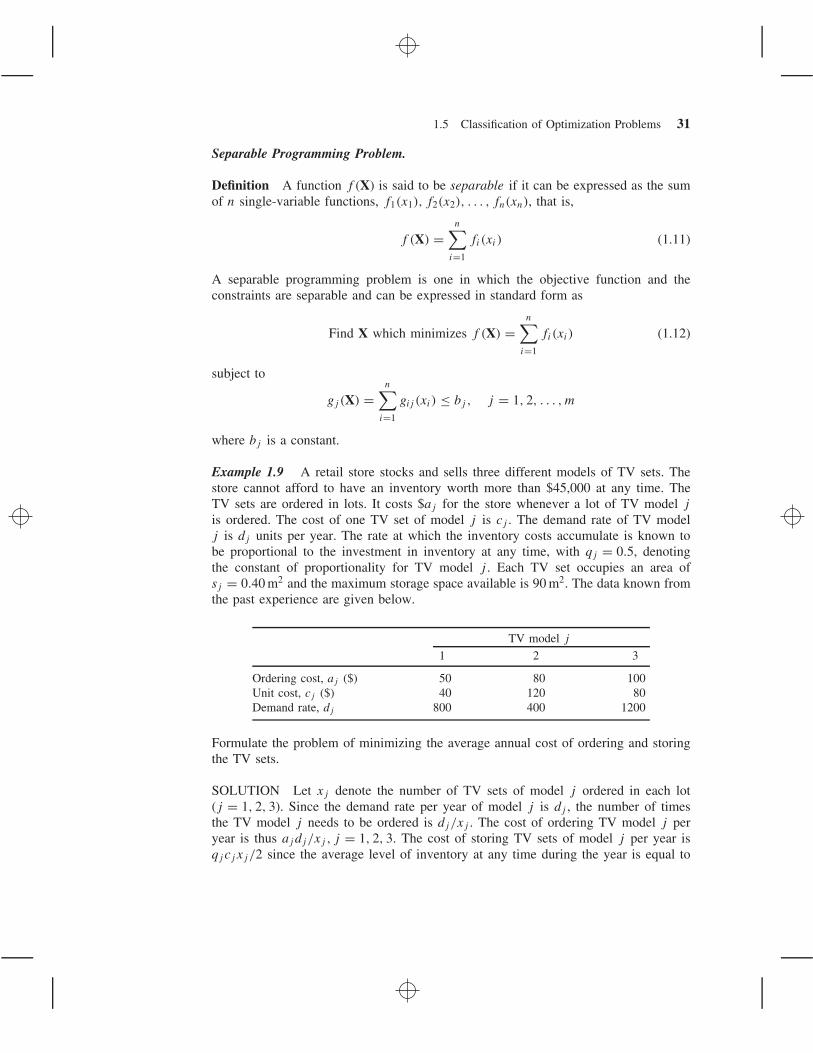
Example 1.9 A retail store stocks and sells three different models of TV sets. Thestore cannot afford to have an inventory worth more than $45,000 at any time. TheTV sets are ordered in lots. It costs $aj for the store whenever a lot of TV model j
is ordered. The cost of one TV set of model j is cj . The demand rate of TV modelj is dj units per year. The rate at which the inventory costs accumulate is known tobe proportional to the investment in inventory at any time, with qj = 0.5, denotingthe constant of proportionality for TV model j . Each TV set occupies an area ofsj = 0.40 m2 and the maximum storage space available is 90 m2. The data known fromthe past experience are given below.
TV model j
1 2 3
Ordering cost, aj ($) 50 80 100Unit cost, cj ($) 40 120 80Demand rate, dj 800 400 1200
Formulate the problem of minimizing the average annual cost of ordering and storingthe TV sets.
SOLUTION Let xj denote the number of TV sets of model j ordered in each lot(j = 1, 2, 3). Since the demand rate per year of model j is dj , the number of timesthe TV model j needs to be ordered is dj/xj . The cost of ordering TV model j peryear is thus ajdj /xj , j = 1, 2, 3. The cost of storing TV sets of model j per year isqj cjxj /2 since the average level of inventory at any time during the year is equal to

32 Introduction to Optimization
cjxj /2. Thus the objective function (cost of ordering plus storing) can be expressedas
f (X) =(
a1d1
x1+ q1c1x1
2
)
+(
a2d2
x2+ q2c2x2
2
)
+(
a3d3
x3+ q3c3x3
2
)
(E1)
where the design vector X is given by
X =
⎧⎪⎨
⎪⎩
x1
x2
x3
⎫⎪⎬
⎪⎭(E2)
The constraint on the worth of inventory can be stated as
c1x1 + c2x2 + c3x3 ≤ 45,000 (E3)
The limitation on the storage area is given by
s1x1 + s2x2 + s3x3 ≤ 90 (E4)
Since the design variables cannot be negative, we have
xj ≥ 0, j = 1, 2, 3 (E5)
By substituting the known data, the optimization problem can be stated as follows:
Find X which minimizes
f (X) =(
40,000
x1+ 10x1
)
+(
32,000
x2+ 30x2
)
+(
120,000
x3+ 20x3
)
(E6)
subject to
g1(X) = 40x1 + 120x2 + 80x3 ≤ 45,000 (E7)
g2(X) = 0.40(x1 + x2 + x3) ≤ 90 (E8)
g3(X) = −x1 ≤ 0 (E9)
g4(X) = −x2 ≤ 0 (E10)
g5(X) = −x3 ≤ 0 (E11)
It can be observed that the optimization problem stated in Eqs. (E6) to (E11) is aseparable programming problem.
1.5.8 Classification Based on the Number of Objective Functions
Depending on the number of objective functions to be minimized, optimization prob-lems can be classified as single- and multiobjective programming problems. Accordingto this classification, the problems considered in Examples 1.1 to 1.9 are single objectiveprogramming problems.

1.5 Classification of Optimization Problems 33
Multiobjective Programming Problem. A multiobjective programming problem canbe stated as follows:
Find X which minimizes f1(X), f2(X), . . . , fk(X)
subject to
gj (X) ≤ 0, j = 1, 2, . . . , m
(1.13)
where f1, f2, . . . , fk denote the objective functions to be minimized simultaneously.
Example 1.10 A uniform column of rectangular cross section is to be constructedfor supporting a water tank of mass M (Fig. 1.14). It is required (1) to minimize themass of the column for economy, and (2) to maximize the natural frequency of trans-verse vibration of the system for avoiding possible resonance due to wind. Formulatethe problem of designing the column to avoid failure due to direct compression andbuckling. Assume the permissible compressive stress to be σmax.
SOLUTION Let x1 = b and x2 = d denote the cross-sectional dimensions of thecolumn. The mass of the column (m) is given by
m = ρbdl = ρlx1x2 (E1)
where ρ is the density and l is the height of the column. The natural frequency oftransverse vibration of the water tank (ω), by treating it as a cantilever beam with atip mass M , can be obtained as [1.118]
ω =[
3EI
(M + 33140m)l3
]1/2
(E2)
Figure 1.14 Water tank on a column.
34 Introduction to Optimization
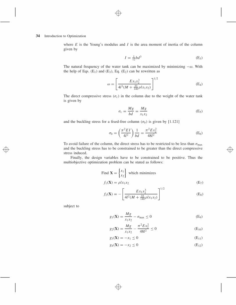
where E is the Young’s modulus and I is the area moment of inertia of the columngiven by
I = 112bd3 (E3)
The natural frequency of the water tank can be maximized by minimizing −ω. Withthe help of Eqs. (E1) and (E3), Eq. (E2) can be rewritten as
ω =[
Ex1x32
4l3(M + 33140ρlx1x2)
]1/2
(E4)
The direct compressive stress (σc) in the column due to the weight of the water tankis given by
σc = Mg
bd= Mg
x1x2(E5)
and the buckling stress for a fixed-free column (σb) is given by [1.121]
σb =(
π2EI
4l2
)1
bd= π2Ex2
2
48l2(E6)
To avoid failure of the column, the direct stress has to be restricted to be less than σmax
and the buckling stress has to be constrained to be greater than the direct compressivestress induced.
Finally, the design variables have to be constrained to be positive. Thus themultiobjective optimization problem can be stated as follows:
Find X ={x1
x2
}
which minimizes
f1(X) = ρlx1x2 (E7)
f2(X) = −[
Ex1x32
4l2(M + 33140ρlx1x2)
]1/2
(E8)
subject to
g1(X) = Mg
x1x2− σmax ≤ 0 (E9)
g2(X) = Mg
x1x2− π2Ex2
2
48l2≤ 0 (E10)
g3(X) = −x1 ≤ 0 (E11)
g4(X) = −x2 ≤ 0 (E12)

1.7 Engineering Optimization Literature 35
1.6 OPTIMIZATION TECHNIQUES
The various techniques available for the solution of different types of optimizationproblems are given under the heading of mathematical programming techniques inTable 1.1. The classical methods of differential calculus can be used to find the uncon-strained maxima and minima of a function of several variables. These methods assumethat the function is differentiable twice with respect to the design variables and thederivatives are continuous. For problems with equality constraints, the Lagrange multi-plier method can be used. If the problem has inequality constraints, the Kuhn–Tuckerconditions can be used to identify the optimum point. But these methods lead to a set ofnonlinear simultaneous equations that may be difficult to solve. The classical methodsof optimization are discussed in Chapter 2.
The techniques of nonlinear, linear, geometric, quadratic, or integer programmingcan be used for the solution of the particular class of problems indicated by the nameof the technique. Most of these methods are numerical techniques wherein an approx-imate solution is sought by proceeding in an iterative manner by starting from aninitial solution. Linear programming techniques are described in Chapters 3 and 4. Thequadratic programming technique, as an extension of the linear programming approach,is discussed in Chapter 4. Since nonlinear programming is the most general methodof optimization that can be used to solve any optimization problem, it is dealt with indetail in Chapters 5–7. The geometric and integer programming methods are discussedin Chapters 8 and 10, respectively. The dynamic programming technique, presented inChapter 9, is also a numerical procedure that is useful primarily for the solution ofoptimal control problems. Stochastic programming deals with the solution of optimiza-tion problems in which some of the variables are described by probability distributions.This topic is discussed in Chapter 11.
In Chapter 12 we discuss calculus of variations, optimal control theory, and opti-mality criteria methods. The modern methods of optimization, including genetic algo-rithms, simulated annealing, particle swarm optimization, ant colony optimization,neural network-based optimization, and fuzzy optimization, are presented in Chapter13. Several practical aspects of optimization are outlined in Chapter 14. The reductionof size of optimization problems, fast reanalysis techniques, the efficient computationof the derivatives of static displacements and stresses, eigenvalues and eigenvectors,and transient response are outlined. The aspects of sensitivity of optimum solution toproblem parameters, multilevel optimization, parallel processing, and multiobjectiveoptimization are also presented in this chapter.
1.7 ENGINEERING OPTIMIZATION LITERATURE
The literature on engineering optimization is large and diverse. Several text-booksare available and dozens of technical periodicals regularly publish papers related toengineering optimization. This is primarily because optimization is applicable to allareas of engineering. Researchers in many fields must be attentive to the developmentsin the theory and applications of optimization.

36 Introduction to Optimization
The most widely circulated journals that publish papers related to engineering opti-mization are Engineering Optimization, ASME Journal of Mechanical Design, AIAAJournal, ASCE Journal of Structural Engineering, Computers and Structures, Interna-tional Journal for Numerical Methods in Engineering, Structural Optimization, Journalof Optimization Theory and Applications, Computers and Operations Research, Oper-ations Research, Management Science, Evolutionary Computation, IEEE Transactionson Evolutionary Computation, European Journal of Operations Research, IEEE Trans-actions on Systems, Man and Cybernetics , and Journal of Heuristics . Many of thesejournals are cited in the chapter references.
1.8 SOLUTION OF OPTIMIZATION PROBLEMS USING MATLAB
The solution of most practical optimization problems requires the use of computers.Several commercial software systems are available to solve optimization problems thatarise in different engineering areas. MATLAB is a popular software that is used forthe solution of a variety of scientific and engineering problems.† MATLAB has severaltoolboxes each developed for the solution of problems from a specific scientific area.The specific toolbox of interest for solving optimization and related problems is calledthe optimization toolbox . It contains a library of programs or m-files, which can beused for the solution of minimization, equations, least squares curve fitting, and relatedproblems. The basic information necessary for using the various programs can be foundin the user’s guide for the optimization toolbox [1.124]. The programs or m-files, alsocalled functions, available in the minimization section of the optimization toolbox aregiven in Table 1.2. The use of the programs listed in Table 1.2 is demonstrated at the endof different chapters of the book. Basically, the solution procedure involves three stepsafter formulating the optimization problem in the format required by the MATLABprogram (or function) to be used. In most cases, this involves stating the objectivefunction for minimization and the constraints in “≤” form with zero or constant valueon the righthand side of the inequalities. After this, step 1 involves writing an m-filefor the objective function. Step 2 involves writing an m-file for the constraints. Step 3involves setting the various parameters at proper values depending on the characteristicsof the problem and the desired output and creating an appropriate file to invoke thedesired MATLAB program (and coupling the m-files created to define the objective andconstraints functions of the problem). As an example, the use of the program, fmincon,for the solution of a constrained nonlinear programming problem is demonstrated inExample 1.11.
Example 1.11 Find the solution of the following nonlinear optimization problem(same as the problem in Example 1.1) using the MATLAB function fmincon:
Minimize f (x1, x2) = 9.82x1x2 + 2x1
subject to
g1(x1, x2) = 2500
πx1x2− 500 ≤ 0
†The basic concepts and procedures of MATLAB are summarized in Appendix C.

1.8 Solution of Optimization Problems Using MATLAB 37
Table 1.2 MATLAB Programs or Functions for Solving Optimization Problems
Name of MATLAB programType of optimization Standard form for solution or function to solveproblem by MATLAB the problem
Function of one variable orscalar minimization
Find x to minimize f (x)
with x1 < x < x2
fminbnd
Unconstrained minimizationof function of severalvariables
Find x to minimize f (x) fminunc or fminsearch
Linear programmingproblem
Find x to minimize fT xsubject to[A]x ≤ b, [Aeq]x = beq,
l ≤ x ≤ u
linprog
Quadratic programmingproblem
Find x to minimize12 xT [H ]x + fT x subject to[A]x ≤ b, [Aeq]x = beq,
l ≤ x ≤ u
quadprog
Minimization of function ofseveral variables subjectto constraints
Find x to minimize f (x)
subject toc(x) ≤ 0, ceq = 0[A]x ≤ b, [Aeq]x = beq,
l ≤ x ≤ u
fmincon
Goal attainment problem Find x and γ to minimize γ
such thatF(x) − wγ ≤ goal,c(x) ≤ 0, ceq = 0[A]x ≤ b, [Aeq]x = beq,
l ≤ x ≤ u
fgoalattain
Minimax problem Minimize Maxx [Fi}
[Fi(x)}such that
c(x) ≤ 0, ceq = 0[A]x ≤ b, [Aeq]x = beq,
l ≤ x ≤ u
fminimax
Binary integer programmingproblem
Find x to minimize fT xsubject to[A]x ≤ b, [Aeq]x = beq,each component of x isbinary
bintprog
g2(x1, x2) = 2500
πx1x2− π2(x2
1 + x22)
0.5882≤ 0
g3(x1, x2) = −x1 + 2 ≤ 0
g4(x1, x2) = x1 − 14 ≤ 0
g5(x1, x2) = −x2 + 0.2 ≤ 0
g6(x1, x2) = x2 − 0.8 ≤ 0

38 Introduction to Optimization
SOLUTION
Step 1 : Write an M-file probofminobj.m for the objective function.
function f= probofminobj (x)f= 9.82*x(1)*x(2)+2*x(1);
Step 2 : Write an M-file conprobformin.m for the constraints.
function [c, ceq] = conprobformin(x)% Nonlinear inequality constraintsc = [2500/(pi*x(1)*x(2))-500;2500/(pi*x(1)*x(2))-(pi^2*(x(1)^2+x(2)^2))/0.5882;-x(1)+2;x(1)-14;-x(2)+0.2;x(2)-0.8];% Nonlinear equality constraintsceq = [];
Step 3 : Invoke constrained optimization program (write this in new matlab file).
clcclear allwarning offx0 = [7 0.4]; % Starting guess\fprintf ('The values of function value and constraintsat starting point\n');f=probofminobj (x0)[c, ceq] = conprobformin (x0)options = optimset ('LargeScale', 'off');[x, fval]=fmincon (@probofminobj, x0, [], [], [], [], [],[], @conprobformin, options)fprintf('The values of constraints at optimum solution\n');[c, ceq] = conprobformin(x) % Check the constraint values at x
This produces the solution or output as follows:
The values of function value and constraints at starting pointf=41.4960c =-215.7947-540.6668-5.0000-7.0000-0.2000-0.4000ceq =[]
Optimization terminated: first-order optimalitymeasure less
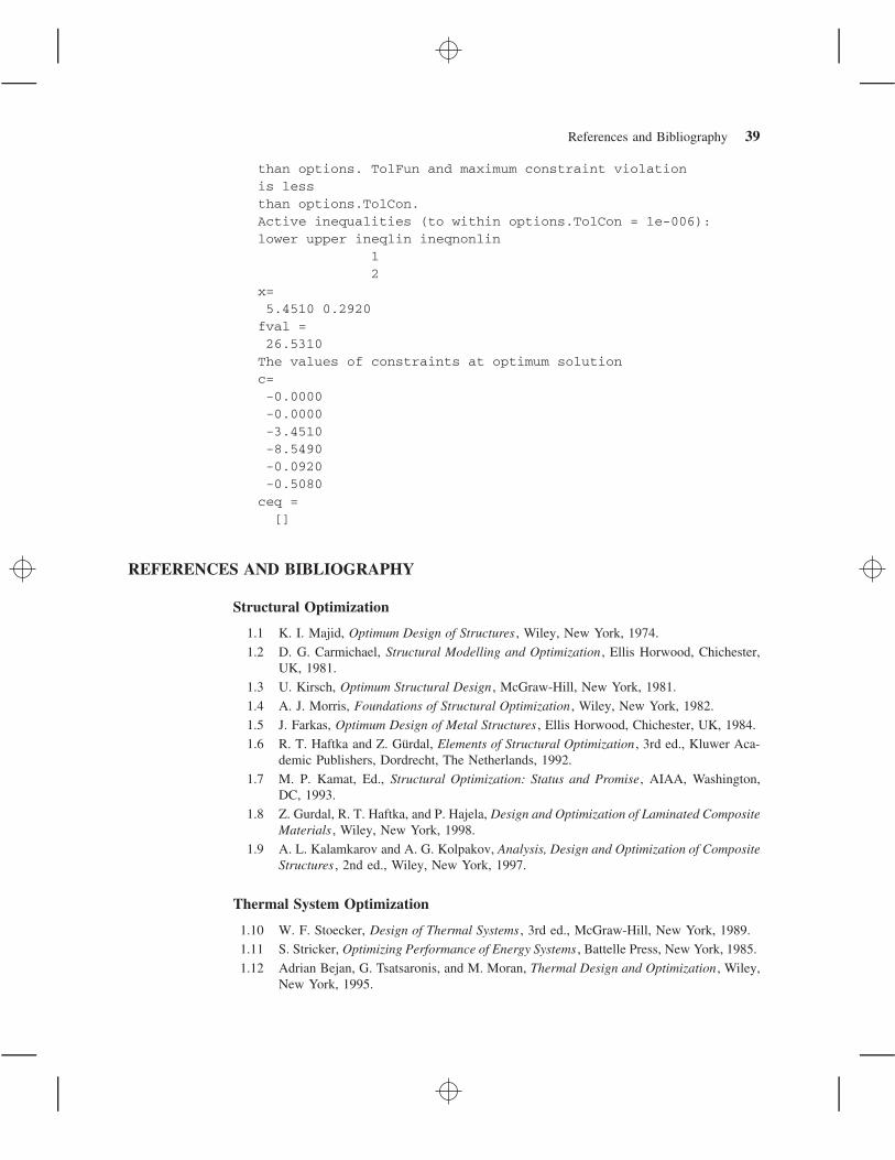
References and Bibliography 39
than options. TolFun and maximum constraint violationis lessthan options.TolCon.Active inequalities (to within options.TolCon = 1e-006):lower upper ineqlin ineqnonlin
12
x=5.4510 0.2920fval =26.5310The values of constraints at optimum solutionc=-0.0000-0.0000-3.4510-8.5490-0.0920-0.5080ceq =[]
REFERENCES AND BIBLIOGRAPHY
Structural Optimization
1.1 K. I. Majid, Optimum Design of Structures , Wiley, New York, 1974.
1.2 D. G. Carmichael, Structural Modelling and Optimization , Ellis Horwood, Chichester,UK, 1981.
1.3 U. Kirsch, Optimum Structural Design , McGraw-Hill, New York, 1981.
1.4 A. J. Morris, Foundations of Structural Optimization , Wiley, New York, 1982.
1.5 J. Farkas, Optimum Design of Metal Structures , Ellis Horwood, Chichester, UK, 1984.
1.6 R. T. Haftka and Z. Gurdal, Elements of Structural Optimization , 3rd ed., Kluwer Aca-demic Publishers, Dordrecht, The Netherlands, 1992.
1.7 M. P. Kamat, Ed., Structural Optimization: Status and Promise, AIAA, Washington,DC, 1993.
1.8 Z. Gurdal, R. T. Haftka, and P. Hajela, Design and Optimization of Laminated CompositeMaterials , Wiley, New York, 1998.
1.9 A. L. Kalamkarov and A. G. Kolpakov, Analysis, Design and Optimization of CompositeStructures , 2nd ed., Wiley, New York, 1997.
Thermal System Optimization
1.10 W. F. Stoecker, Design of Thermal Systems , 3rd ed., McGraw-Hill, New York, 1989.
1.11 S. Stricker, Optimizing Performance of Energy Systems , Battelle Press, New York, 1985.
1.12 Adrian Bejan, G. Tsatsaronis, and M. Moran, Thermal Design and Optimization , Wiley,New York, 1995.

40 Introduction to Optimization
1.13 Y. Jaluria, Design and Optimization of Thermal Systems , 2nd ed., CRC Press, BocaRaton, FL, 2007.
Chemical and Metallurgical Process Optimization
1.14 W. H. Ray and J. Szekely, Process Optimization with Applications to Metallurgy andChemical Engineering , Wiley, New York, 1973.
1.15 T. F. Edgar and D. M. Himmelblau, Optimization of Chemical Processes , McGraw-Hill,New York, 1988.
1.16 R. Aris, The Optimal Design of Chemical Reactors, a Study in Dynamic Programming ,Academic Press, New York, 1961.
Electronics and Electrical Engineering
1.17 K. W. Cattermole and J. J. O’Reilly, Optimization Methods in Electronics and Commu-nications , Wiley, New York, 1984.
1.18 T. R. Cuthbert, Jr., Optimization Using Personal Computers with Applications to Elec-trical Networks , Wiley, New York, 1987.
1.19 G. D. Micheli, Synthesis and Optimization of Digital Circuits , McGraw-Hill, New York,1994.
Mechanical Design
1.20 R. C. Johnson, Optimum Design of Mechanical Elements , Wiley, New York, 1980.
1.21 E. J. Haug and J. S. Arora, Applied Optimal Design: Mechanical and Structural Systems ,Wiley, New York, 1979.
1.22 E. Sevin and W. D. Pilkey, Optimum Shock and Vibration Isolation , Shock and VibrationInformation Center, Washington, DC, 1971.
General Engineering Design
1.23 J. Arora, Introduction to Optimum Design , 2nd ed., Academic Press, San Diego, 2004.
1.24 P. Y. Papalambros and D. J. Wilde, Principles of Optimal Design , Cambridge UniversityPress, Cambridge, UK, 1988.
1.25 J. N. Siddall, Optimal Engineering Design: Principles and Applications , Marcel Dekker,New York, 1982.
1.26 S. S. Rao, Optimization: Theory and Applications , 2nd ed., Wiley, New York, 1984.
1.27 G. N. Vanderplaats, Numerical Optimization Techniques for Engineering Design withApplications , McGraw-Hill, New York, 1984.
1.28 R. L. Fox, Optimization Methods for Engineering Design , Addison-Wesley, Reading,MA, 1972.
1.29 A. Ravindran, K. M. Ragsdell, and G. V. Reklaitis, Engineering Optimization: Methodsand Applications , 2nd ed., Wiley, New York, 2006.
1.30 D. J. Wilde, Globally Optimal Design , Wiley, New York, 1978.
1.31 T. E. Shoup and F. Mistree, Optimization Methods with Applications for Personal Com-puters , Prentice-Hall, Englewood Cliffs, NJ, 1987.
1.32 A. D. Belegundu and T. R. Chandrupatla, Optimization Concepts and Applications inEngineering , Prentice Hall, Upper Saddle River, NJ, 1999.
References and Bibliography 41
General Nonlinear Programming Theory
1.33 S. L. S. Jacoby, J. S. Kowalik, and J. T. Pizzo, Iterative Methods for Nonlinear Opti-mization Problems , Prentice-Hall, Englewood Cliffs, NJ, 1972.
1.34 L. C. W. Dixon, Nonlinear Optimization: Theory and Algorithms , Birkhauser, Boston,1980.
1.35 G. S. G. Beveridge and R. S. Schechter, Optimization: Theory and Practice,McGraw-Hill, New York, 1970.
1.36 B. S. Gottfried and J. Weisman, Introduction to Optimization Theory , Prentice-Hall,Englewood Cliffs, NJ, 1973.
1.37 M. A. Wolfe, Numerical Methods for Unconstrained Optimization , Van Nostrand Rein-hold, New York, 1978.
1.38 M. S. Bazaraa and C. M. Shetty, Nonlinear Programming , Wiley, New York, 1979.
1.39 W. I. Zangwill, Nonlinear Programming: A Unified Approach , Prentice-Hall, EnglewoodCliffs, NJ, 1969.
1.40 J. E. Dennis and R. B. Schnabel, Numerical Methods for Unconstrained Optimizationand Nonlinear Equations , Prentice-Hall, Englewood Cliffs, NJ, 1983.
1.41 J. S. Kowalik, Methods for Unconstrained Optimization Problems , American Elsevier,New York, 1968.
1.42 A. V. Fiacco and G. P. McCormick, Nonlinear Programming: Sequential UnconstrainedMinimization Techniques , Wiley, New York, 1968.
1.43 G. Zoutendijk, Methods of Feasible Directions , Elsevier, Amsterdam, 1960.
1.44 J. Nocedal and S. J. Wright, Numerical Optimization , Springer, New York, 2006.
1.45 R. Fletcher, Practical Methods of Optimization , Vols. 1 and 2, Wiley, Chichester, UK,1981.
1.46 D. P. Bertsekas, Nonlinear Programming , 2nd ed., Athena Scientific, Nashua, NH,1999.
1.47 D. G. Luenberger, Linear and Nonlinear Programming , 2nd ed., Kluwer AcademicPublishers, Norwell, MA, 2003.
1.48 A. Antoniou and W-S. Lu, Practical Optimization: Algorithms and Engineering Appli-cations , Springer, Berlin, 2007.
1.49 S. G. Nash and A. Sofer, Linear and Nonlinear Programming , McGraw-Hill, New York,1996.
Computer Programs
1.50 J. L. Kuester and J. H. Mize, Optimization Techniques with Fortran , McGraw-Hill, NewYork, 1973.
1.51 H. P. Khunzi, H. G. Tzschach, and C. A. Zehnder, Numerical Methods of Mathemati-cal Optimization with ALGOL and FORTRAN Programs , Academic Press, New York,1971.
1.52 C. S. Wolfe, Linear Programming with BASIC and FORTRAN , Reston Publishing Co.,Reston, VA, 1985.
1.53 K. R. Baker, Optimization Modeling with Spreadsheets , Thomson Brooks/Cole, Belmont,CA, 2006.
1.54 P. Venkataraman, Applied Optimization with MATLAB Programming , Wiley, New York,2002.
42 Introduction to Optimization
Optimal Control
1.55 D. E. Kirk, Optimal Control Theory: An Introduction , Prentice-Hall, Englewood Cliffs,NJ, 1970.
1.56 A. P. Sage and C. C. White III, Optimum Systems Control , 2nd ed., Prentice-Hall,Englewood Cliffs, NJ, 1977.
1.57 B. D. O. Anderson and J. B. Moore, Linear Optimal Control , Prentice-Hall, EnglewoodCliffs, NJ, 1971.
1.58 A. E. Bryson and Y. C. Ho, Applied Optimal Control: Optimization, Estimation, andControl , Blaisdell, Waltham, MA, 1969.
Geometric Programming
1.59 R. J. Duffin, E. L. Peterson, and C. Zener, Geometric Programming: Theory and Appli-cations , Wiley, New York, 1967.
1.60 C. M. Zener, Engineering Design by Geometric Programming , Wiley, New York, 1971.
1.61 C. S. Beightler and D. T. Phillips, Applied Geometric Programming , Wiley, New York,1976.
1.62 B-Y. Cao, Fuzzy Geometric Programming , Kluwer Academic, Dordrecht, The Nether-lands, 2002.
1.63 A. Paoluzzi, Geometric Programming for Computer-aided Design , Wiley, New York,2003.
Linear Programming
1.64 G. B. Dantzig, Linear Programming and Extensions , Princeton University Press, Prince-ton, NJ, 1963.
1.65 S. Vajda, Linear Programming: Algorithms and Applications , Methuen, New York,1981.
1.66 S. I. Gass, Linear Programming: Methods and Applications , 5th ed., McGraw-Hill, NewYork, 1985.
1.67 C. Kim, Introduction to Linear Programming , Holt, Rinehart, & Winston, New York,1971.
1.68 P. R. Thie, An Introduction to Linear Programming and Game Theory , Wiley, NewYork, 1979.
1.69 S. I. Gass, An illustrated Guide to Linear Programming , Dover, New York, 1990.
1.70 K. G. Murty, Linear Programming , Wiley, New York, 1983.
Integer Programming
1.71 T. C. Hu, Integer Programming and Network Flows , Addison-Wesley, Reading, MA,1982.
1.72 A. Kaufmann and A. H. Labordaere, Integer and Mixed Programming: Theory andApplications , Academic Press, New York, 1976.
1.73 H. M. Salkin, Integer Programming , Addison-Wesley, Reading, MA, 1975.
1.74 H. A. Taha, Integer Programming: Theory, Applications, and Computations , AcademicPress, New York, 1975.
1.75 A. Schrijver, Theory of Linear and Integer Programming , Wiley, New York, 1998.

References and Bibliography 43
1.76 J. K. Karlof (Ed.), Integer Programming: Theory and Practice, CRC Press, Boca Raton,FL, 2006.
1.77 L. A. Wolsey, Integer Programming , Wiley, New York, 1998.
Dynamic Programming
1.78 R. Bellman, Dynamic Programming , Princeton University Press, Princeton, NJ, 1957.
1.79 R. Bellman and S. E. Dreyfus, Applied Dynamic Programming , Princeton UniversityPress, Princeton, NJ, 1962.
1.80 G. L. Nemhauser, Introduction to Dynamic Programming , Wiley, New York, 1966.
1.81 L. Cooper and M. W. Cooper, Introduction to Dynamic Programming , Pergamon Press,Oxford, UK, 1981.
1.82 W. B. Powell, Approximate Dynamic Programming: Solving the Curses of Dimension-ality , Wiley, Hoboken, NJ, 2007.
1.83 M. L. Puterman, Dynamic Programming and Its Applications , Academic Press, NewYork, 1978.
1.84 M. Sniedovich, Dynamic Programming , Marcel Dekker, New York, 1992.
Stochastic Programming
1.85 J. K. Sengupta, Stochastic Programming: Methods and Applications , North-Holland,Amsterdam, 1972.
1.86 P. Kall, Stochastic Linear Programming , Springer-Verlag, Berlin, 1976.
1.87 J. R. Birge and F. Louveaux, Introduction to Stochastic Programming , Springer, NewYork, 1997.
1.88 P. Kall and S. W. Wallace, Stochastic Programming , Wiley, Chichester, UK, 1994.
1.89 P. Kall and J. Mayer, Stochastic Linear Programming: Models, Theory, and Computa-tion , Springer, New York, 2005.
Multiobjective Programming
1.90 R. E. Steuer, Multiple Criteria Optimization: Theory, Computation, and Application ,Wiley, New York, 1986.
1.91 C. L. Hwang and A. S. M. Masud, Multiple Objective Decision Making: Methodsand Applications , Lecture Notices in Economics and Mathematical Systems, Vol. 164,Springer-Verlag, Berlin, 1979.
1.92 J. P. Ignizio, Linear Programming in Single and Multi-objective Systems , Prentice-Hall,Englewood Cliffs, NJ, 1982.
1.93 A. Goicoechea, D. R. Hansen, and L. Duckstein, Multiobjective Decision Analysis withEngineering and Business Applications , Wiley, New York, 1982.
1.94 Y. Collette and P. Siarry, Multiobjective Optimization: Principles and Case Studies ,Springer, Berlin, 2004.
1.95 H. Eschenauer, J. Koski, and A. Osyczka (Eds.), Multicriteria Design Optimization:Procedures and Applications , Springer-Verlag, Berlin, 1990.
1.96 P. Sen and J-B. Yang, Multiple Criteria Decision Support in Engineering Design ,Springer-Verlag, Berlin, 1998.
1.97 G. Owen, Game Theory , 3rd ed., Academic Press, San Diego, 1995.

44 Introduction to Optimization
Nontraditional Optimization Techniques
1.98 M. Mitchell, An Introduction to Genetic Algorithms , MIT Press, Cambridge, MA, 1998.
1.99 D. B. Fogel, Evolutionary Computation: Toward a New Philosophy of Machine Intelli-gence, 3rd ed., IEEE Press, Piscataway, NJ, 2006.
1.100 K. Deb, Multi-Objective Optimization Using Evolutionary Algorithms , Wiley, Chich-ester, England, 2001.
1.101 C. A. Coello Coello, D. A. van Veldhuizen and G. B. Lamont, Evolutionary Algorithmsfor Solving Multi-Objective Problems , Plenum, New York, 2002.
1.102 D. E. Goldberg, Genetic Algorithms in Search, Optimization and Machine Learning ,Addison-Wesley, Reading, MA, 1989.
1.103 P. J. M. van Laarhoven and E. Aarts, Simulated Annealing: Theory and Applications ,D. Reidel, Dordrecht, The Netherlands, 1987.
1.104 J. Hopfield and D. Tank, “Neural Computation of Decisions in Optimization Problems,”Biological Cybernetics , Vol. 52, pp. 141–152, 1985.
1.105 J. J. Hopfield, Neural networks and physical systems with emergent collective compu-tational abilities, Proceedings of the National Academy of Sciences, USA, Vol. 79, pp.2554–2558, 1982.
1.106 N. Forbes, Imitation of Life: How Biology Is Inspiring Computing , MIT Press, Cam-bridge, MA, 2004.
1.107 J. Harris, Fuzzy Logic Applications in Engineering Science, Springer, Dordrecht, TheNetherlands, 2006.
1.108 M. Hanss, Applied Fuzzy Arithmetic: An Introduction with Engineering Applications ,Springer, Berlin, 2005.
1.109 G. Chen and T. T. Pham, Introduction to Fussy Systems , Chapman & Hall/CRC, BocaRaton, FL, 2006.
1.110 T. J. Ross, Fuzzy Logic with Engineering Applications , McGraw-Hill, New York, 1995.
1.111 M. Dorigo and T. Stutzle, Ant Colony Optimization , MIT Press, Cambridge, MA, 2004.
1.112 J. Kennedy, R. C. Eberhart, and Y. Shi, Swarm Intelligence, Morgan Kaufmann, SanFrancisco, CA, 2001.
1.113 J. C. Spall, Introduction to Stochastic Search and Optimization , Wiley Interscience,2003.
1.114 A. P. Engelbrecht, Fundamentals of Computational Swarm Intelligence, Wiley, Chich-ester, UK, 2005.
1.115 E. Bonabeau, M. Dorigo, and G. Theraulaz, Swarm Intelligence: From Natural to Arti-ficial Systems , Oxford University Press, Oxford, UK, 1999.
Additional References
1.116 R. C. Juvinall and K. M. Marshek, Fundamentals of Machine Component Design , 2nded., Wiley, New York, 1991.
1.117 J. E. Shigley and C. R. Mischke, Mechanical Engineering Design , 5th ed., McGraw-Hill,New York, 1989.
1.118 S. S. Rao, Mechanical Vibrations , 4th ed., Pearson Prentice Hall, Upper Saddle River,NJ, 2004.
1.119 J. M. MacGregor, Reinforced Concrete: Mechanics and Design , Prentice Hall, Engle-wood Cliffs, NJ, 1988.
1.120 S. S. Rao, Reliability-Based Design , McGraw-Hill, New York, 1992.

Review Questions 45
1.121 N. H. Cook, Mechanics and Materials for Design , McGraw-Hill, New York, 1984.
1.122 R. Ramarathnam and B. G. Desai, Optimization of polyphase induction motor design: anonlinear programming approach, IEEE Transactions on Power Apparatus and Systems ,Vol. PAS-90, No. 2, pp. 570–578, 1971.
1.123 R. M. Stark and R. L. Nicholls, Mathematical Foundations for Design: Civil EngineeringSystems , McGraw-Hill, New York, 1972.
1.124 T. F. Coleman, M. A. Branch, and A. Grace, Optimization Toolbox—for Use withMATLAB®, User’s Guide, Version 2 MathWorks Inc., Natick, MA, 1999.
REVIEW QUESTIONS1.1 Match the following terms and descriptions:
(a) Free feasible point gj (X) = 0(b) Free infeasible point Some gj (X) = 0 and other gj (X) < 0(c) Bound feasible point Some gj (X) = 0 and other gj (X) ≥ 0(d) Bound infeasible point Some gj (X) > 0 and other gj (X) < 0(e) Active constraints All gj (X) < 0
1.2 Answer true or false:
(a) Optimization problems are also known as mathematical programming problems.
(b) The number of equality constraints can be larger than the number of design variables.
(c) Preassigned parameters are part of design data in a design optimization problem.
(d) Side constraints are not related to the functionality of the system.
(e) A bound design point can be infeasible.
(f) It is necessary that some gj (X) = 0 at the optimum point.
(g) An optimal control problem can be solved using dynamic programming techniques.
(h) An integer programming problem is same as a discrete programming problem.
1.3 Define the following terms:
(a) Mathematical programming problem
(b) Trajectory optimization problem
(c) Behavior constraint
(d) Quadratic programming problem
(e) Posynomial
(f) Geometric programming problem
1.4 Match the following types of problems with their descriptions.
(a) Geometric programming problem Classical optimization problem(b) Quadratic programming problem Objective and constraints are quadratic(c) Dynamic programming problem Objective is quadratic and constraints are linear(d) Nonlinear programming problem Objective and constraints arise from a serial
system(e) Calculus of variations problem Objective and constraints are polynomials with
positive coefficients
1.5 How do you solve a maximization problem as a minimization problem?

46 Introduction to Optimization
1.6 State the linear programming problem in standard form.
1.7 Define an OC problem and give an engineering example.
1.8 What is the difference between linear and nonlinear programming problems?
1.9 What is the difference between design variables and preassigned parameters?
1.10 What is a design space?
1.11 What is the difference between a constraint surface and a composite constraint surface?
1.12 What is the difference between a bound point and a free point in the design space?
1.13 What is a merit function?
1.14 Suggest a simple method of handling multiple objectives in an optimization problem.
1.15 What are objective function contours?
1.16 What is operations research?
1.17 State five engineering applications of optimization.
1.18 What is an integer programming problem?
1.19 What is graphical optimization, and what are its limitations?
1.20 Under what conditions can a polynomial in n variables be called a posynomial?
1.21 Define a stochastic programming problem and give two practical examples.
1.22 What is a separable programming problem?
PROBLEMS
1.1 A fertilizer company purchases nitrates, phosphates, potash, and an inert chalk base at acost of $1500, $500, $1000, and $100 per ton, respectively, and produces four fertilizersA, B,C, and D. The production cost, selling price, and composition of the four fertilizersare given below.
Percentage composition by weightProduction Sellingcost price Inert
Fertilizer ($/ton) ($/ton) Nitrates Phosphates Potash chalk base
A 100 350 5 10 5 80B 150 550 5 15 10 70C 200 450 10 20 10 60D 250 700 15 5 15 65
During any week, no more than 1000 tons of nitrate, 2000 tons of phosphates, and1500 tons of potash will be available. The company is required to supply a minimumof 5000 tons of fertilizer A and 4000 tons of fertilizer D per week to its customers;but it is otherwise free to produce the fertilizers in any quantities it pleases. Formulatethe problem of finding the quantity of each fertilizer to be produced by the company tomaximize its profit.

Problems 47
Figure 1.15 Two-bar truss.
1.2 The two-bar truss shown in Fig. 1.15 is symmetric about the y axis. The nondimensionalarea of cross section of the members A/Aref, and the nondimensional position of joints1 and 2, x/h, are treated as the design variables x1 and x2, respectively, where Aref
is the reference value of the area (A) and h is the height of the truss. The coordinatesof joint 3 are held constant. The weight of the truss (f1) and the total displacement ofjoint 3 under the given load (f2) are to be minimized without exceeding the permissiblestress, σ0. The weight of the truss and the displacement of joint 3 can be expressed as
f1(X) = 2ρhx2
√
1 + x21Aref
f2(X) =Ph(1 + x2
1 )1.5√
1 + x41
2√
2Ex21x2Aref
where ρ is the weight density, P the applied load, and E the Young’s modulus. Thestresses induced in members 1 and 2 (σ1 and σ2) are given by
σ1(X) =P(1 + x1)
√
(1 + x21 )
2√
2x1x2Aref
σ2(X) =P(x1 − 1)
√
(1 + x21 )
2√
2x1x2Aref
In addition, upper and lower bounds are placed on design variables x1 and x2 as
xmini ≤ xi ≤ xmax
i ; i = 1, 2
Find the solution of the problem using a graphical method with (a) f1 as the objective, (b) f2
as the objective, and (c) (f1 + f2) as the objective for the following data: E = 30 × 106 psi,
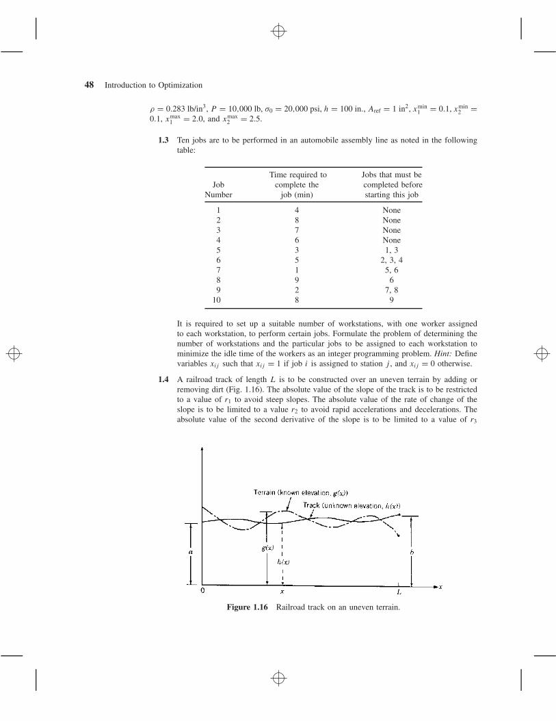
48 Introduction to Optimization
ρ = 0.283 lb/in3, P = 10,000 lb, σ0 = 20,000 psi, h = 100 in., Aref = 1 in2, xmin1 = 0.1, xmin
2 =0.1, xmax
1 = 2.0, and xmax2 = 2.5.
1.3 Ten jobs are to be performed in an automobile assembly line as noted in the followingtable:
Time required to Jobs that must beJob complete the completed before
Number job (min) starting this job
1 4 None2 8 None3 7 None4 6 None5 3 1, 36 5 2, 3, 47 1 5, 68 9 69 2 7, 8
10 8 9
It is required to set up a suitable number of workstations, with one worker assignedto each workstation, to perform certain jobs. Formulate the problem of determining thenumber of workstations and the particular jobs to be assigned to each workstation tominimize the idle time of the workers as an integer programming problem. Hint: Definevariables xij such that xij = 1 if job i is assigned to station j , and xij = 0 otherwise.
1.4 A railroad track of length L is to be constructed over an uneven terrain by adding orremoving dirt (Fig. 1.16). The absolute value of the slope of the track is to be restrictedto a value of r1 to avoid steep slopes. The absolute value of the rate of change of theslope is to be limited to a value r2 to avoid rapid accelerations and decelerations. Theabsolute value of the second derivative of the slope is to be limited to a value of r3
Figure 1.16 Railroad track on an uneven terrain.

Problems 49
to avoid severe jerks. Formulate the problem of finding the elevation of the track tominimize the construction costs as an OC problem. Assume the construction costs to beproportional to the amount of dirt added or removed. The elevation of the track is equalto a and b at x = 0 and x = L, respectively.
1.5 A manufacturer of a particular product produces x1 units in the first week and x2 unitsin the second week. The number of units produced in the first and second weeks mustbe at least 200 and 400, respectively, to be able to supply the regular customers. Theinitial inventory is zero and the manufacturer ceases to produce the product at the endof the second week. The production cost of a unit, in dollars, is given by 4x2
i , where xi
is the number of units produced in week i(i = 1, 2). In addition to the production cost,there is an inventory cost of $10 per unit for each unit produced in the first week thatis not sold by the end of the first week. Formulate the problem of minimizing the totalcost and find its solution using a graphical optimization method.
1.6 Consider the slider-crank mechanism shown in Fig. 1.17 with the crank rotating ata constant angular velocity ω. Use a graphical procedure to find the lengths of thecrank and the connecting rod to maximize the velocity of the slider at a crank angle ofθ = 30◦ for ω = 100 rad/s. The mechanism has to satisfy Groshof’s criterion l ≥ 2.5r
to ensure 360◦ rotation of the crank. Additional constraints on the mechanism are givenby 0.5 ≤ r ≤ 10, 2.5 ≤ l ≤ 25, and 10 ≤ x ≤ 20.
1.7 Solve Problem 1.6 to maximize the acceleration (instead of the velocity) of the slider atθ = 30◦ for ω = 100 rad/s.
1.8 It is required to stamp four circular disks of radii R1, R2, R3, and R4 from a rectan-gular plate in a fabrication shop (Fig. 1.18). Formulate the problem as an optimizationproblem to minimize the scrap. Identify the design variables, objective function, and theconstraints.
1.9 The torque transmitted (T ) by a cone clutch, shown in Fig. 1.19, under uniform pressurecondition is given by
T = 2πfp
3 sin α(R3
1 − R32)
where p is the pressure between the cone and the cup, f the coefficient of friction, α
the cone angle, R1 the outer radius, and R2 the inner radius.
(a) Find R1 and R2 that minimize the volume of the cone clutch with α = 30◦,
F = 30 lb, and f = 0.5 under the constraints T ≥ 100 lb-in., R1 ≥ 2R2,0 ≤ R1 ≤ 15 in., and 0 ≤ R2 ≤ 10 in.
Figure 1.17 Slider-crank mechanism.
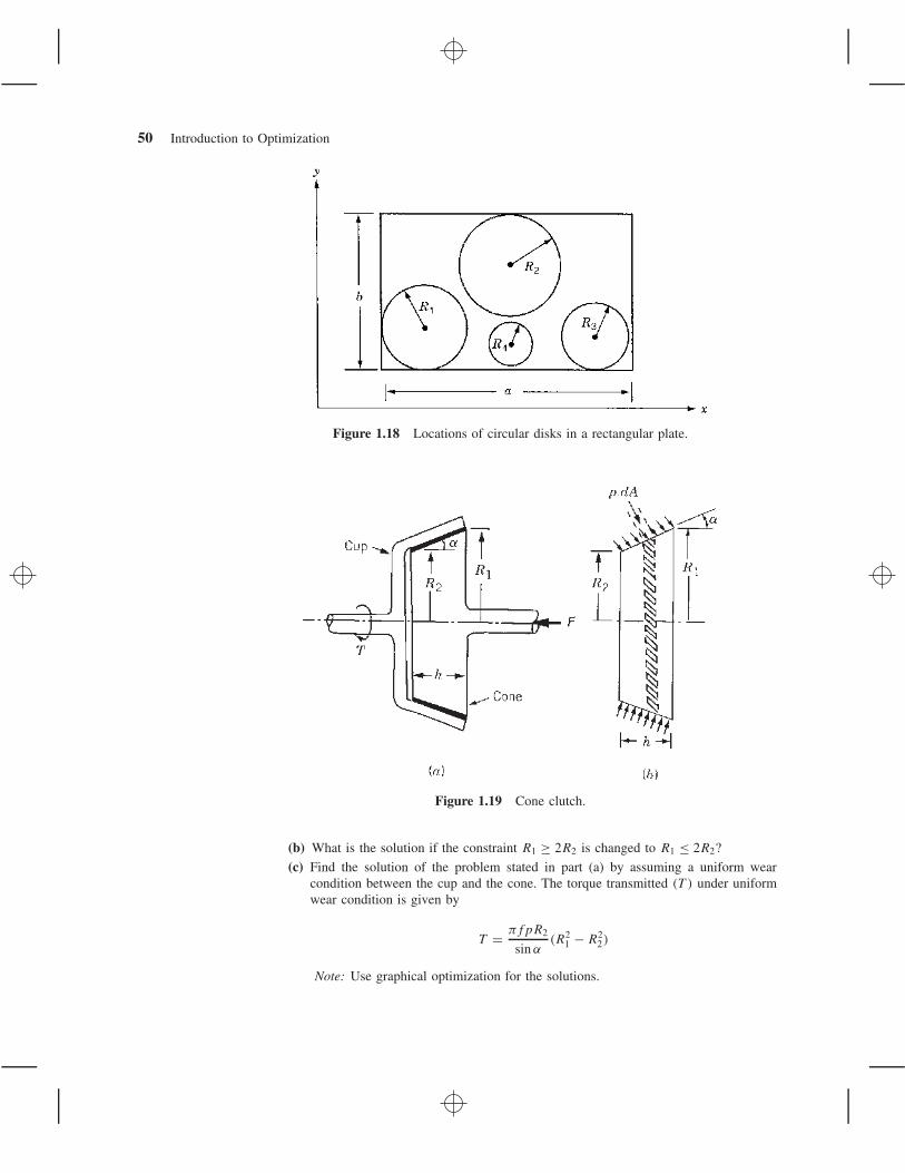
50 Introduction to Optimization
Figure 1.18 Locations of circular disks in a rectangular plate.
Figure 1.19 Cone clutch.
(b) What is the solution if the constraint R1 ≥ 2R2 is changed to R1 ≤ 2R2?
(c) Find the solution of the problem stated in part (a) by assuming a uniform wearcondition between the cup and the cone. The torque transmitted (T ) under uniformwear condition is given by
T = πfpR2
sin α(R2
1 − R22)
Note: Use graphical optimization for the solutions.

Problems 51
1.10 A hollow circular shaft is to be designed for minimum weight to achieve a minimumreliability of 0.99 when subjected to a random torque of (T , σT ) = (106, 104) lb-in.,where T is the mean torque and σT is the standard deviation of the torque, T . Thepermissible shear stress, τ0, of the material is given by (τ 0, στ0) = (50,000, 5000) psi,where τ 0 is the mean value and στ0 is the standard deviation of τ0. The maximuminduced stress (τ ) in the shaft is given by
τ = T ro
J
where ro is the outer radius and J is the polar moment of inertia of the cross sectionof the shaft. The manufacturing tolerances on the inner and outer radii of the shaft arespecified as ±0.06 in. The length of the shaft is given by 50 ± 1 in. and the specificweight of the material by 0.3 ± 0.03 lb/in3. Formulate the optimization problem andsolve it using a graphical procedure. Assume normal distribution for all the randomvariables and 3σ values for the specified tolerances. Hints: (1) The minimum reliabilityrequirement of 0.99 can be expressed, equivalently, as [1.120]
z1 = 2.326 ≤ τ − τ 0√
σ 2τ + σ 2
τ0
(2) If f (x1, x2, . . . , xn) is a function of the random variables x1, x2, . . . , xn, the meanvalue of f (f ) and the standard deviation of f (σf ) are given by
f = f (x1, x2, . . . , xn)
σf =⎡
⎣n∑
i=1
(∂f
∂xi
∣∣∣∣x1,x2,...,xn
)2
σ 2xi
⎤
⎦
1/2
where xi is the mean value of xi , and σxi is the standard deviation of xi .
1.11 Certain nonseparable optimization problems can be reduced to a separable form byusing suitable transformation of variables. For example, the product term f = x1x2 canbe reduced to the separable form f = y2
1 − y22 by introducing the transformations
y1 = 12 (x1 + x2), y2 = 1
2 (x1 − x2)
Suggest suitable transformations to reduce the following terms to separable form:
(a) f = x21x3
2 , x1 > 0, x2 > 0
(b) f = xx21 , x1 > 0
1.12 In the design of a shell-and-tube heat exchanger (Fig. 1.20), it is decided to have the totallength of tubes equal to at least α1 [1.10]. The cost of the tube is α2 per unit length andthe cost of the shell is given by α3D
2.5L, where D is the diameter and L is the length ofthe heat exchanger shell. The floor space occupied by the heat exchanger costs α4 per unitarea and the cost of pumping cold fluid is α5L/d5N2 per day, where d is the diameterof the tube and N is the number of tubes. The maintenance cost is given by α6NdL.The thermal energy transferred to the cold fluid is given by α7/N
1.2dL1.4 + α8/d0.2L.
Formulate the mathematical programming problem of minimizing the overall cost of theheat exchanger with the constraint that the thermal energy transferred be greater thana specified amount α9. The expected life of the heat exchanger is α10 years. Assumethat αi, i = 1, 2, . . . , 10, are known constants, and each tube occupies a cross-sectionalsquare of width and depth equal to d .

52 Introduction to Optimization
Figure 1.20 Shell-and-tube heat exchanger.
Figure 1.21 Electrical bridge network.
1.13 The bridge network shown in Fig. 1.21 consists of five resistors Ri(i = 1, 2, . . . , 5).If Ii is the current flowing through the resistance Ri , the problem is to find the resistancesR1, R2, . . . , R5 so that the total power dissipated by the network is a minimum. Thecurrent Ii can vary between the lower and upper limits Ii,min and Ii,max, and the voltagedrop, Vi = RiIi , must be equal to a constant ci for 1 ≤ i ≤ 5. Formulate the problem asa mathematical programming problem.
1.14 A traveling saleswoman has to cover n towns. She plans to start from a particular townnumbered 1, visit each of the other n − 1 towns, and return to the town 1. The distancebetween towns i and j is given by dij . Formulate the problem of selecting the sequencein which the towns are to be visited to minimize the total distance traveled.
1.15 A farmer has a choice of planting barley, oats, rice, or wheat on his 200-acre farm. Thelabor, water, and fertilizer requirements, yields per acre, and selling prices are given inthe following table:
Labor Water Fertilizer SellingType of cost required required Yield pricecrop ($) (m3) (lb) (lb) ($/lb)
Barley 300 10,000 100 1,500 0.5Oats 200 7,000 120 3,000 0.2Rice 250 6,000 160 2,500 0.3Wheat 360 8,000 200 2,000 0.4
The farmer can also give part or all of the land for lease, in which case he gets $200 peracre. The cost of water is $0.02/m3 and the cost of the fertilizer is $2/lb. Assume thatthe farmer has no money to start with and can get a maximum loan of $50,000 from theland mortgage bank at an interest of 8 %. He can repay the loan after six months. The

Problems 53
irrigation canal cannot supply more than 4 × 10⁵ m3 of water. Formulate the problem offinding the planting schedule for maximizing the expected returns of the farmer.
1.16 There are two different sites, each with four possible targets (or depths) to drill an oilwell. The preparation cost for each site and the cost of drilling at site i to target j aregiven below:
Drilling cost to target j
Site i 1 2 3 4 Preparation cost
1 4 1 9 7 112 7 9 5 2 13
Formulate the problem of determining the best site for each target so that the total costis minimized.
1.17 A four-pole dc motor, whose cross section is shown in Fig. 1.22, is to be designed withthe length of the stator and rotor x1, the overall diameter of the motor x2, the unnotchedradius x3, the depth of the notches x4, and the ampere turns x5 as design variables.
Figure 1.22 Cross section of an idealized motor.

54 Introduction to Optimization
The air gap is to be less than k1√
x2 + 7.5 where k1 is a constant. The temperature ofthe external surface of the motor cannot exceed T above the ambient temperature.Assuming that the heat can be dissipated only by radiation, formulate the problem formaximizing the power of the motor [1.59]. Hints:
1. The heat generated due to current flow is given by k2x1x−12 x−1
4 x25 , where k2 is a
constant. The heat radiated from the external surface for a temperature difference of T is given by k3x1x2 T , where k3 is a constant.
2. The expression for power is given by k4NBx1x3x5, where k4 is a constant, N is therotational speed of the rotor, and B is the average flux density in the air gap.
3. The units of the various quantities are as follows. Lengths: centimeter, heat generated,heat dissipated; power: watt; temperature: ◦C; rotational speed: rpm; flux density:gauss.
1.18 A gas pipeline is to be laid between two cities A and E, making it pass through oneof the four locations in each of the intermediate towns B,C, and D (Fig. 1.23). Theassociated costs are indicated in the following tables.
Costs for A to B and D to E
Station i
1 2 3 4
From A to point i of B 30 35 25 40From point i of D to E 50 40 35 25
Costs for B to C and C to D
To:
From: 1 2 3 4
1 22 18 24 182 35 25 15 213 24 20 26 204 22 21 23 22
Figure 1.23 Possible paths of the pipeline between A and E.

Problems 55
Figure 1.24 Beam-column.
Formulate the problem of minimizing the cost of the pipeline.
1.19 A beam-column of rectangular cross section is required to carry an axial load of 25 lband a transverse load of 10 lb, as shown in Fig. 1.24. It is to be designed to avoid thepossibility of yielding and buckling and for minimum weight. Formulate the optimizationproblem by assuming that the beam-column can bend only in the vertical (xy) plane.Assume the material to be steel with a specific weight of 0.3 lb/in3, Young’s modulus of30 × 106 psi, and a yield stress of 30,000 psi. The width of the beam is required to be atleast 0.5 in. and not greater than twice the depth. Also, find the solution of the problemgraphically. Hint: The compressive stress in the beam-column due to Py is Py/bd andthat due to Px is
Pxld
2Izz
= 6Pxl
bd2
The axial buckling load is given by
(Py)cri = π2EIzz
4l2= π2Ebd3
48l2
1.20 A two-bar truss is to be designed to carry a load of 2W as shown in Fig. 1.25. Bothbars have a tubular section with mean diameter d and wall thickness t . The materialof the bars has Young’s modulus E and yield stress σy . The design problem involvesthe determination of the values of d and t so that the weight of the truss is a minimumand neither yielding nor buckling occurs in any of the bars. Formulate the problem as anonlinear programming problem.
Figure 1.25 Two-bar truss.

56 Introduction to Optimization
Figure 1.26 Processing plant layout (coordinates in ft).
1.21 Consider the problem of determining the economic lot sizes for four different items.Assume that the demand occurs at a constant rate over time. The stock for theith item is replenished instantaneously upon request in lots of sizes Qi . The totalstorage space available is A, whereas each unit of item i occupies an area di . Theobjective is to find the values of Qi that optimize the per unit cost of holding theinventory and of ordering subject to the storage area constraint. The cost function isgiven by
C =4∑
i=1
(ai
Qi
+ biQi
)
, Qi > 0
where ai and bi are fixed constants. Formulate the problem as a dynamic programming(optimal control) model. Assume that Qi is discrete.
1.22 The layout of a processing plant, consisting of a pump (P ), a water tank (T ), a com-pressor (C), and a fan (F ), is shown in Fig. 1.26. The locations of the various units, interms of their (x, y) coordinates, are also indicated in this figure. It is decided to add anew unit, a heat exchanger (H), to the plant. To avoid congestion, it is decided to locateH within a rectangular area defined by {−15 ≤ x ≤ 15,−10 ≤ y ≤ 10}. Formulate theproblem of finding the location of H to minimize the sum of its x and y distances fromthe existing units, P, T ,C, and F .
1.23 Two copper-based alloys (brasses), A and B, are mixed to produce a new alloy, C.The composition of alloys A and B and the requirements of alloy C are given in thefollowing table:

Problems 57
Composition by weight
Alloy Copper Zinc Lead Tin
A 80 10 6 4B 60 20 18 2C ≥ 75 ≥ 15 ≥ 16 ≥ 3
If alloy B costs twice as much as alloy A, formulate the problem of determining theamounts of A and B to be mixed to produce alloy C at a minimum cost.
1.24 An oil refinery produces four grades of motor oil in three process plants. The refineryincurs a penalty for not meeting the demand of any particular grade of motor oil. Thecapacities of the plants, the production costs, the demands of the various grades of motoroil, and the penalties are given in the following table:
Production cost ($/day) tomanufacture motor oil of grade:Process Capacity of the plant
plant (kgal/day) 1 2 3 4
1 100 750 900 1000 12002 150 800 950 1100 14003 200 900 1000 1200 1600
Demand (kgal/day) 50 150 100 75Penalty (per each kilogallon shortage) $10 $12 $16 $20
Formulate the problem of minimizing the overall cost as an LP problem.
1.25 A part-time graduate student in engineering is enrolled in a four-unit mathematics courseand a three-unit design course. Since the student has to work for 20 hours a week at alocal software company, he can spend a maximum of 40 hours a week to study outsidethe class. It is known from students who took the courses previously that the numericalgrade (g) in each course is related to the study time spent outside the class as gm = tm/6and gd = td/5, where g indicates the numerical grade (g = 4 for A, 3 for B, 2 for C, 1 forD, and 0 for F), t represents the time spent in hours per week to study outside the class,and the subscripts m and d denote the courses, mathematics and design, respectively.The student enjoys design more than mathematics and hence would like to spend at least75 minutes to study for design for every 60 minutes he spends to study mathematics.Also, as far as possible, the student does not want to spend more time on any coursebeyond the time required to earn a grade of A. The student wishes to maximize his gradepoint P , given by P = 4gm + 3gd , by suitably distributing his study time. Formulatethe problem as an LP problem.
1.26 The scaffolding system, shown in Fig. 1.27, is used to carry a load of 10,000 lb. Assumingthat the weights of the beams and the ropes are negligible, formulate the problem ofdetermining the values of x1, x2, x3, and x4 to minimize the tension in ropes A and B
while maintaining positive tensions in ropes C, D,E, and F .
1.27 Formulate the problem of minimum weight design of a power screw subjected to anaxial load, F , as shown in Fig. 1.28 using the pitch (p), major diameter (d), nut height

58 Introduction to Optimization
Figure 1.27 Scaffolding system.
Figure 1.28 Power screw.
(h), and screw length (s) as design variables. Consider the following constraints in theformulation:
1. The screw should be self-locking [1.117].
2. The shear stress in the screw should not exceed the yield strength of the material inshear. Assume the shear strength in shear (according to distortion energy theory), tobe 0.577σy , where σy is the yield strength of the material.
3. The bearing stress in the threads should not exceed the yield strength of the material,σy .
4. The critical buckling load of the screw should be less than the applied load, F .
1.28 (a) A simply supported beam of hollow rectangular section is to be designed for mini-mum weight to carry a vertical load Fy and an axial load P as shown in Fig. 1.29.The deflection of the beam in the y direction under the self-weight and Fy should
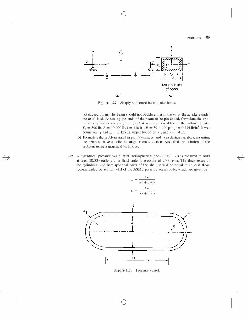
Problems 59
Figure 1.29 Simply supported beam under loads.
not exceed 0.5 in. The beam should not buckle either in the yz or the xz plane underthe axial load. Assuming the ends of the beam to be pin ended, formulate the opti-mization problem using xi, i = 1, 2, 3, 4 as design variables for the following data:Fy = 300 lb, P = 40,000 lb, l = 120 in., E = 30 × 106 psi, ρ = 0.284 lb/in3, lowerbound on x1 and x2 = 0.125 in, upper bound on x1, and x2 = 4 in.
(b) Formulate the problem stated in part (a) using x1 and x2 as design variables, assumingthe beam to have a solid rectangular cross section. Also find the solution of theproblem using a graphical technique.
1.29 A cylindrical pressure vessel with hemispherical ends (Fig. 1.30) is required to holdat least 20,000 gallons of a fluid under a pressure of 2500 psia. The thicknesses ofthe cylindrical and hemispherical parts of the shell should be equal to at least thoserecommended by section VIII of the ASME pressure vessel code, which are given by
tc = pR
Se + 0.4p
th = pR
Se + 0.8p
Figure 1.30 Pressure vessel.
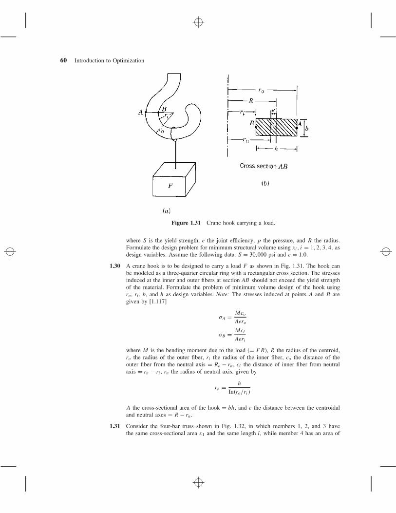
60 Introduction to Optimization
Figure 1.31 Crane hook carrying a load.
where S is the yield strength, e the joint efficiency, p the pressure, and R the radius.Formulate the design problem for minimum structural volume using xi, i = 1, 2, 3, 4, asdesign variables. Assume the following data: S = 30,000 psi and e = 1.0.
1.30 A crane hook is to be designed to carry a load F as shown in Fig. 1.31. The hook canbe modeled as a three-quarter circular ring with a rectangular cross section. The stressesinduced at the inner and outer fibers at section AB should not exceed the yield strengthof the material. Formulate the problem of minimum volume design of the hook usingro, ri , b, and h as design variables. Note: The stresses induced at points A and B aregiven by [1.117]
σA = Mco
Aero
σB = Mci
Aeri
where M is the bending moment due to the load (= FR), R the radius of the centroid,ro the radius of the outer fiber, ri the radius of the inner fiber, co the distance of theouter fiber from the neutral axis = Ro − rn, ci the distance of inner fiber from neutralaxis = rn − ri , rn the radius of neutral axis, given by
rn = h
In(ro/ri)
A the cross-sectional area of the hook = bh, and e the distance between the centroidaland neutral axes = R − rn.
1.31 Consider the four-bar truss shown in Fig. 1.32, in which members 1, 2, and 3 havethe same cross-sectional area x1 and the same length l, while member 4 has an area of

Problems 61
Figure 1.32 Four-bar truss.
cross section x2 and length√
3 l. The truss is made of a lightweight material for whichYoung’s modulus and the weight density are given by 30 × 106 psi and 0.03333 lb/in3,respectively. The truss is subject to the loads P1 = 10,000 lb and P2 = 20,000 lb. Theweight of the truss per unit value of l can be expressed as
f = 3x1(1)(0.03333) + x2
√3(0.03333) = 0.1x1 + 0.05773x2
The vertical deflection of joint A can be expressed as
δA = 0.6
x1+ 0.3464
x2
and the stresses in members 1 and 4 can be written as
σ1 = 5(10,000)
x1= 50,000
x1, σ4 = −2
√3(10,000)
x2= −34,640
x2
The weight of the truss is to be minimized with constraints on the vertical deflection ofthe joint A and the stresses in members 1 and 4. The maximum permissible deflectionof joint A is 0.1 in. and the permissible stresses in members are σmax = 8333.3333 psi(tension) and σmin = −4948.5714 psi (compression). The optimization problem can bestated as a separable programming problem as follows:
Minimize f (x1, x2) = 0.1x1 + 0.05773x2
subject to0.6
x1+ 0.3464
x2− 0.1 ≤ 0, 6 − x1 ≤ 0, 7 − x2 ≤ 0
Determine the solution of the problem using a graphical procedure.
1.32 A simply supported beam, with a uniform rectangular cross section, is subjected to bothdistributed and concentrated loads as shown in Fig. 1.33. It is desired to find the crosssection of the beam to minimize the weight of the beam while ensuring that the maximumstress induced in the beam does not exceed the permissible stress (σ0) of the materialand the maximum deflection of the beam does not exceed a specified limit (δ0).The data of the problem are P = 105 N, p0 = 106 N/m, L = 1 m, E = 207 GPa, weightdensity (ρw) = 76.5 kN/m3, σ0 = 220 MPa, and δ0 = 0.02 m.

62 Introduction to Optimization
x2
x1
p0 per unit length
Cross-section
P
L
L2
Figure 1.33 A simply supported beam subjected to concentrated and distributed loads.
(a) Formulate the problem as a mathematical programming problem assuming thatthe cross-sectional dimensions of the beam are restricted as x1 ≤ x2, 0.04m ≤ x1
≤ 0.12m, and 0.06m ≤ x2 ≤ 0.20 m.
(b) Find the solution of the problem formulated in part (a) using MATLAB.
(c) Find the solution of the problem formulated in part (a) graphically.
1.33 Solve Problem 1.32, parts (a), (b), and (c), assuming the cross section of the beam tobe hollow circular with inner diameter x1 and outer diameter x2. Assume the data andbounds on the design variables to be as given in Problem 1.32.
1.34 Find the solution of Problem 1.31 using MATLAB.
1.35 Find the solution of Problem 1.2(a) using MATLAB.
1.36 Find the solution of Problem 1.2(b) using MATLAB.