Introduction to Parallel Algorithms(DRAFT)

Guy E. Blelloch, Laxman Dhulipala and Yihan Sun

March 13, 2021

Contents

1 Introduction 3

2 Models 3

3 Preliminaries 9

4 Some Building Blocks 124.1 Scan . . . . . . . . . . . . . . . . . . . . . . . . . . . . . . . . . . . . . 124.2 Filter and Flatten . . . . . . . . . . . . . . . . . . . . . . . . . . . . . . 154.3 Search . . . . . . . . . . . . . . . . . . . . . . . . . . . . . . . . . . . . 154.4 Merge . . . . . . . . . . . . . . . . . . . . . . . . . . . . . . . . . . . . 174.5 K-th Smallest . . . . . . . . . . . . . . . . . . . . . . . . . . . . . . . . 184.6 Summary . . . . . . . . . . . . . . . . . . . . . . . . . . . . . . . . . . 20

5 Sorting 205.1 Mergesort . . . . . . . . . . . . . . . . . . . . . . . . . . . . . . . . . . 205.2 Quicksort . . . . . . . . . . . . . . . . . . . . . . . . . . . . . . . . . . 215.3 Sample Sort . . . . . . . . . . . . . . . . . . . . . . . . . . . . . . . . . 235.4 Counting and Radix Sort . . . . . . . . . . . . . . . . . . . . . . . . . . 235.5 Semisort . . . . . . . . . . . . . . . . . . . . . . . . . . . . . . . . . . . 24

6 Graph Algorithms 256.1 Graph primitives . . . . . . . . . . . . . . . . . . . . . . . . . . . . . . 266.2 Parallel breadth-first search . . . . . . . . . . . . . . . . . . . . . . . . 266.3 Low-diameter decomposition . . . . . . . . . . . . . . . . . . . . . . . . 276.4 Connectivity . . . . . . . . . . . . . . . . . . . . . . . . . . . . . . . . . 316.5 Spanners . . . . . . . . . . . . . . . . . . . . . . . . . . . . . . . . . . . 316.6 Maximal Independent Set . . . . . . . . . . . . . . . . . . . . . . . . . 32

1

7 Parallel Binary Trees 357.1 Preliminaries . . . . . . . . . . . . . . . . . . . . . . . . . . . . . . . . 357.2 The join Algorithms for Each Balancing Scheme . . . . . . . . . . . . . 36

7.2.1 AVL Trees . . . . . . . . . . . . . . . . . . . . . . . . . . . . . . 377.2.2 Red-black Trees . . . . . . . . . . . . . . . . . . . . . . . . . . . 387.2.3 Weight Balanced Trees . . . . . . . . . . . . . . . . . . . . . . . 417.2.4 Treaps . . . . . . . . . . . . . . . . . . . . . . . . . . . . . . . . 43

7.3 Algorithms Using join . . . . . . . . . . . . . . . . . . . . . . . . . . . 447.3.1 Two Helper Functions: split and join2 . . . . . . . . . . . . . . 44

7.4 Set-set Functions Using join . . . . . . . . . . . . . . . . . . . . . . . . 467.5 Other Tree algorithms Using join . . . . . . . . . . . . . . . . . . . . . 48

8 Other Models and Simulations 518.1 PRAM . . . . . . . . . . . . . . . . . . . . . . . . . . . . . . . . . . . . 528.2 Simulations . . . . . . . . . . . . . . . . . . . . . . . . . . . . . . . . . 528.3 The Scheduling Problem . . . . . . . . . . . . . . . . . . . . . . . . . . 528.4 Greedy Scheduling . . . . . . . . . . . . . . . . . . . . . . . . . . . . . 538.5 Work Stealing Schedulers . . . . . . . . . . . . . . . . . . . . . . . . . . 54

2

1 Introduction

This document is intended an introduction to parallel algorithms. The algorithmsand techniques described in this document cover over 40 years of work by hundreds ofresearchers. The earliest work on parallel algorithms dates back to the 1970s. The keyideas of the parallel merging algorithm described in Section 4.4, for example, appearin a 1975 paper by Leslie Valiant, a Turing Award winner. Many other Turing awardwinners have contributed to ideas in this document including Richard Karp, RobertTarjan, and John Hopcroft.

The focus of this document is on key ideas which have survived or are likely tosurvive the test of time, and are likely to be useful in designing parallel algorithms nowand far into the future.

Although this document is focused on the theory of parallel algorithms, many, ifnot most, of the algorithms and algorithmic techniques in this document have beenimplemented on modern multicore machines (e.g., your laptop, iphone, or server).The algorithms most often, sometimes with tweaks, far outperform the best sequentialalgorithms on the same machine, even ones with a modest number of cores.

This document is a work in progress. Please tell us about any bugs youfind and give us feedback on the presentation.

2 Models

To analyze the cost of algorithms, it is important to have a concrete model with awell-defined notion of costs. Sequentially, it is well-known that the Random AccessMachine (RAM) model has served well for many years. The RAM model is meantto approximate how real sequential machines work. It consists of a single processorwith some constant number of registers, an instruction counter and an arbitrarily largememory. The instructions include register-to-register instructions (e.g. adding thecontents of two registers and putting the result in a third), control-instructions (e.g.jumping), and the ability to read from and write to arbitrary locations in memory. Forthe purpose of analyzing cost, the RAM model assumes that all instructions take unittime. The “time” (cost) of a computation is then just the total number of instructionsit performs from the start until a final end instruction. To allow storing a pointerto memory in a register or memory location, but disallow playing games by storingarbitrary large values, most often it is assumed that for an input of size n, each registerand memory location can store Θ(log n) bits.

The RAM is by no stretch meant to model the runtime on a real machine with cycle-by-cycle level accuracy. It does not model, for example, that modern-day machineshave cache hierarchies and therefore not all memory accesses are equally expensive.Modeling all features of modern-day machines would lead to very complicated modelsthat could be hard to use and hard to gain intuition from. Instead the RAM tries to besimple. As such the RAM does not precisely model the performance of any particular

3

real machine, it can, and has, effectively served to compare different algorithms, andunderstand how the performance of the algorithms will scale with size. For thesereasons the RAM model should really only be used for asymptotic (i.e. big-O) analysis.The RAM has also served as a tool to better understand algorithmic techniques suchas divide-and-conquer, and dynamic programming, among many others. Finally, andimportantly, it is natural to write pseudocode or real code that is naturally translatedto the RAM.

In the context of parallel algorithms, we would like to use a cost model that sat-isfies the same important features—i.e., simple, guides the user to the most efficientalgorithms, helps the user understand how an algorithm scales with input size, robustacross a variety of machines, helps the user understand algorithmic techniques, and canbe naturally expressed with simple pseudocode and real code. Early work on parallelalgorithms largely used the Parallel RAM (PRAM) model [20]. The model consistsof p fully synchronous processors accessing a shared memory. Costs are measured interms of the number of processors and the number of time steps. Unfortunately thePRAM is not particularly well suited for simple pseudocode, and consequently realcode, due to its assumption of a fixed number of processors—the user needs to worryabout allocating tasks to processors.

More recently researchers have used so-called work-span (or work-depth) models inwhich algorithms still assume a shared random access memory, but allow dynamicallycreating tasks (or processes). Costs are measured in terms of the total number ofoperations, the work and the longest chain of dependences (the depth or the span).This simplifies the description and analysis of algorithms—avoiding the need to talkabout scheduling tasks to processors.

In this document we use a work-span model, the MP-RAM, which we feel perhapsbest satisfies the the features for a good parallel algorithmic model. It is based on theRAM, but allows the dynamic forking of new processes. Fortunately costs are robustwhether analyzed in the PRAM and MP-RAM (and other models). If we define workin the PRAM as the product of the number of processors and the time, almost allalgorithms in this document have the same work in the PRAM or MP-RAM. If wedefine span in the PRAM as time, then all algorithms in this document have a span inthe PRAM that differs by at most a logarithmic factor from the MP-RAM.

It may not be obvious how to map these dynamic processes onto a physical machinewhich will only have a fixed number of processors. To convince ourselves that it ispossible, later we show how to design schedulers that map the processes onto processors,and prove bounds that relate costs. In particular we show various forms of the followingwork-span, processor-time relationship:

max

(W

P,D

)≤ T ≤ O

(W

P+D

)(1)

where W is the work, D the span, P the processors, and T the running time usingP processors. More details on other models and simulations among them is given inSection ??

4

When evaluating parallel computations, we are especially interested in the twoquantities work and span, because they each reflects an aspect of the parallel computa-tion. The work, as indicated by its definition, is equivalent to the running time of thesame computation on one processor (or, sequentially). One might be curious about whywe need to care about the sequential time complexity for a parallel algorithm. Firstof all, the total work still indicates how much resource the computation needs, includethe computational ability, power, etc. More importantly, from the running time pointof view, the total work affects the time in the W/P term (see equation 1). In modernmulticore machines, the number of processors P is usually small compared to the workW , as it is usually Ω(n) for input size n. Meanwhile, often D is asymptotically muchsmaller than W (see more details below). This makes the running time bound to bedominated by the total work W . We call a parallel algorithm work-efficient, if itswork is work asymptotically the same as its best-known sequential counterpart. Whendesign parallel algorithms, our goal is usually to make the algorithm work-efficient, orat least close to work-efficient.

The span for a parallel algorithm reflects another aspect of the computation, thatis, what is the running time when you have an infinite number of processors. In otherwords, this is a “lower bound” of running time whatever the number of processors.Although as mentioned above, the running time is usually bounded by work W , thespan indicates an algorithm’s ability to gain better performance on more processors.This is also referred to as the scalability of the algorithm 1. Intuitively, when design-ing parallel algorithms, the goal in terms of span is to not let it dominate the cost.Generally speaking, we would like to bound the span to be polylogarithmic in n.

Another measure that can be derived from the work and span is parallelism, whichis defined simply as the work divided by the span. It indicates, asymptotically speak-ing, how many processors can be effectively used by the computation. If the workequals span then the parallelism is 1 and the computation is sequential. If the workis O(n log n) and the span is O(log2 n) then the parallelism is O(n/ log n) which isactually quite high, and unlikely to be a bottleneck on most machines in the next 25years. If the work is O(n2) and the span is O(n) then the parallelism is O(n), which iseven higher, even though the span is not polylogarithmic.

In summary, the primary focus should be on designing work-efficient algorithmswith good parallelism, and, ideally but not necessarily, with polylogarithmic span.

The work-span model is a simple cost model, which specifies how the total costof the algorithm should be evaluated. It does not specify, however, what operationsare allowed or disallowed in a parallel computation, e.g., what type of concurrencyor synchronization is supported. In the following, we introduce the MP-RAM model,which will be the main model used in this book.

1In many other settings, scalability means the ability to gain good performance when the inputsize increases. In parallel algorithms, especially in this book, we use this term to mean the ability togain performance when the number of processors increases.

5

MP-RAM

The Multi-Process Random-Access Machine (MP-RAM) consists of a set of processesthat share an unbounded memory. Each process runs the instructions of a RAM—itworks on a program stored in memory, has its own program counter, a constant numberof its own registers, and runs standard RAM instructions. The MP-RAM extends theRAM with a fork instruction that takes a positive integer k and forks k new childprocesses. Each child process receives a unique integer in the range [1, . . . , k] in its firstregister and otherwise has the identical state as the parent (forking process), whichhas that register set to 0. All children start by running the next instruction, and theparent suspends until all the children terminate (execute an end instruction). Thefirst instruction of the parent after all children terminate is called the join instruction.A computation starts with a single root process and finishes when that root processends. This model supports nested parallelism—the ability to fork processes in a nestedfashion. If the root process never does a fork, it is a standard sequential program.

A computation in the MP-RAM defines a partial order on the instructions. Inparticular (1) every instruction depends on its previous instruction in the same thread(if any), (2) every first instruction in a process depends on the fork instruction of theparent that generated it, and (3) every join instruction depends on the end instructionof all child processes of the corresponding fork generated. These dependences definethe partial order. The work of a computation is the total number of instructions, andthe span is the longest sequences of dependent instructions. As usual, the partial ordercan be viewed as a DAG. For a fork of a set of child processes and corresponding jointhe span of the subcomputation is the maximum of the span of the child processes, andthe work is the sum. This property is useful for analyzing algorithms, and specificallyfor writing recurrences for determining work and span.

We assume that the results of memory operations are consistent with some totalorder (linearization) on the instructions that preserves the partial order—i.e., a readwill return the value of the previous write to the same location in the total order. Thechoice of total order can affect the results of a program since processes can communicatethrough the shared memory. In general, therefore computations can be nondetermin-istic. Two instructions are said to be concurrent if they are unordered, and orderedotherwise. Two instructions conflict if one writes to a memory location that the otherreads or writes the same location. We say two instructions race if they are concurrentand conflict. If there are no races in a computation, and no other sources of non-determinism, then all linearized orders will return the same result. This is because allpairs of conflicting instructions are ordered by the partial order (otherwise it wouldbe a race) and hence must appear in the same relative order in all linearizations. Aparticular linearized order is to iterate sequentially from the first to last child in eachfork. We call this the sequential ordering.

Pseudocode. Our pseudocode will look like standard sequential code, except for theaddition of two constructs for expressing parallelism. The first construct is a parallel

6

loop indicated with parFor. For example the following loop applies a function f toeach element of an array A, writing the result into an array B:

parfor i in [0 : |A|]B[i]← f(A[i])

In pseudocode [s : e] means the sequence of integers from s (inclusive) to e (exclusive),and← means assignment. Our arrays are zero based. A parallel loop over n iterationscan easily be implemented in the MP-RAM by forking n children applying the loopbody in each child and then ending each child. The work of a parallel loop is the sumof the work of the loop bodies. The span is the maximum of the span of the loopbodies.

The second construct is a parallel do, which just runs some number of statements inparallel. In pseudocode we use a semicolon to express sequential ordering of statementsand double bars (||) to express parallel statements. For example the following code willsum the elements of an array.

sum(A) =if (|A| = 1) then return A[0]elsel← sum(A[0 : |A|/2]) ‖r ← sum(A[|A|/2 : |A|]);return l + r

The || construct in the code indicates that the two statements with recursive calls tosum should be done in parallel. The semicolon before the return indicates that the twoparallel recursive calls have to complete before adding the results. In our pseudocode weuse the A[s : e] notation to indicate the slice of an array between location s (inclusive)and e (exclusive). If s (or e) is empty it indicates the slice starts (finishes) at thebeginning (end) of the array. Taking a slices takes O(1) work and span since it needonly keep track of the offsets.

The || construct directly maps to a fork in the MP-RAM, in which the first andsecond child run the two statements. Analogously to parFor, the work of a || is thesum of the work of the statements, and the span is the maximum of the spans of thestatements. For the sum example the overall work can be written as the recurrence:

W (n) = W (n/2) +W (n/2) +O(1) = 2W (n/2) +O(1)

which solves to O(n), and the span as

D(n) = max(D(n/2), D(n/2) +O(1) = D(n/2) +O(1)

which solves to O(log n).It is important to note that parallel-for loops and parallel-do (||) instructions can

be nested in an arbitrary fashion.

7

Binary or Arbitrary Forking. Some of our algorithms use just binary forkingwhile others use arbitrary n-way forking. This makes some difference when we discussscheduling the MP-RAM onto a fixed number of processors, and can make a differencein the span bounds. We will use the term the binary-forking MP-RAM, or binary-forking model for short, to indicate the version that only allows binary forking. Insome cases we give separate bounds for MP-RAM and binary forking model. It isalways possible to implement n-way forking using binary forking by creating a tree ofbinary forks of span log n. Thus in general this can increase the span, but not alwaysdoes so. In these cases we will use parfor2 to indicate we are using a tree to fork then parallel calls.

Scheduling. Clearly the MP-RAM is an abstract model since one cannot just createnew processors by calling a fork instruction. In reality the processes of the MP-RAMhave to be scheduled onto actual processors on the machine. This is the job of ascheduler. The scheduler needs to keep some kind of work queue and then distributethe work to processors. When forking, new tasks (processes) are added to the queue,and when a processor finishes its task, it goes to the queue for more work. Here we use“queue” in a generic sence since it could implemented in a distributed fashion, and itmight be first-in first-out, or last-in last out, or an arbitrary combination.

Implementing schedulers will be a topic of later chapters, and will be used to showbounds such as given in Equation 1.

Additional Instructions. In the parallel context it is useful to add some additionalinstructions that manipulate memory. Some commonly-used instructions are a test-and-set (TS), compare-and-swap (CAS), fetch-and-add (FA), and priority-write (PW).These primitives are atomic, meaning that they are indivisible. Even when executedconcurrently with other instructions, these primitives will either be correctly completed,or as if not executed (does not affect the shared memory state). These instructions aresupported by most modern architecture, either directly or indirectly. We discuss ourmodel with one of these operations enabled as the TS-, FA-, and PW-variants of theMP-RAM.

A testAndSet(x) (TS) instruction takes a reference to a memory location x,checks if the value of x is false and if so atomically sets it to true and returns true;if already true it returns false.

A compareAndSwap(x, o, n) (CAS) instruction takes a reference to a memorylocation x, checks if the value of x equals o. If so, the instruction will change the valueto n and return true. If not, the instruction does nothing and simply returns false.

A fetchAndAdd(x, y) (FA) instruction takes a reference to a memory location x,and a value y, and it adds y to the value of x, returning the old value. Different froma TS or a CAS, an FA instruction always successfully adds y to the value stored in x.

A priorityWrite(x, y) (PW) instruction takes a reference to a memory locationx, and checks if the value y is less than the current value in x. If so, it changes the

8

value stored in x to y, and return true. If not, it does nothing and return false.For the operations above returning a boolean value (TS, CAS and PW), we say it

succeeds (or is successful) if it returns a true, and otherwise it fails (or is unsuccessful).It is worth noting that some of these instructions can be used to implement some

other instructions, and thus more powerful, while some of them cannot. Usually, TS isconsidered to be the weakest instruction, as it cannot be used to simulate any of theother instructions. On the other hand, the other three can all be used to simulate TS.

Memory Allocation. To simplify issues of parallel memory allocation we assumethere is an allocate instruction that takes a positive integer n and allocates a con-tiguous block of n memory locations, returning a pointer to the block, and a freeinstruction that given a pointer to an allocated block, frees it.

3 Preliminaries

We will make significant use of randomized algorithms in this document and assumesome reasonable understanding of probability theory (e.g., random variables, expecta-tions, independence, conditional probability, union bound, Markov’s inequality). Weare often interested in tail bounds of probability distributions, and showing that theprobability of some tail is very small—i.e. the cumulative probability above somethreshold value in a probability density function is very small. Hence the cumulativeprobability not in this tail is very high, approaching 1.

These tail bounds are often asymptotic as a function of some parameter n. Inparticular we will use the following definiton for “high probability”.

Definition 3.1 (w.h.p.). g(n) ∈ O(f(n)) with high probability (w.h.p.) if g(n) ∈O(cf(n)) with probability at least 1−

(1n

)c, for some constant c0 and all c ≥ c0.

This definition allows us to make the probability arbitrarily close to 1 by increasingc, and even for a modest constant c (e.g. 3), the probability is very close to 1.

Such high-probability, or tail, bounds are particularly important in parallel algo-rithms since we often cannot effectively use expectations. In a sequential algorithm weare just adding times so we can compose the times taken by a bunch of componentsby adding their expected times and relying on the linearity of expectations to get theoverall expected time. In parallel we often run multiple components in parallel andwait for the last to finish. Therefore the overal span is the maximum of the spans ofthe components, not the sum.

Unfortunately there is no equivalent to linearity of expectations for maximums.Instead a common approach is to show that the probability that each component willnot finish within some span is very small. The union bound tells us that if we sum theseprobabilities, this is an upper bound on the probability that any will not finish withinthat bound. The goals is therefore to then show that this sum is still sufficiently small.The polynomial (1/n)c term in the high probability bound is important since when we

9

multiply this possibility of not being within the bounds by n parallel components, wehave that the probability of them all being within our bounds is at least 1 + (1/n)c−1.This is sufficient since we can use any constant c.

There are many ways to derive tail bounds, many based on Chernoff or Hoeffdingbounds. In this document we will mostly use the following rather simple inequality fortail bounds.

Theorem 3.1. Consider a set of indicator random variables X1, . . . Xn for whichp(Xi = 1) ≤ pi conditioned on all possible events Xj = 0, 1, i 6= j. Let X =

∑ni=1Xi

and E[X] =∑n

i=1 pi, then:

Pr[X ≥ k] ≤(eE[X]

k

)k.

Proof. Let’s first consider the special case that the pi are all equal and have value p. IfX ≥ k then we have that at least k of the random variables are 1. The probability ofany particular k variables all being 1, and the others being anything, is upper boundedby pk. Now we use the union bound over the

(nk

)possible choices of k variables, yielding:

Pr[X ≥ k] ≤ pk(n

k

)< pk

(nek

)k=(pnek

)k=

(eE[X]

k

)kHere we used a standard upper bound on the binomial coefficients:

(nm

)<(nem

)m.

Now consider the case when the pi are not equal. The claim is that making themunequal can only decrease the total bound on probability. This can be seen by startingwith all equal probabilities and then moving some probability from one variable toanother. Some of the k subsets will include both variables, and these probabilitieswill go down since if a set of non-negative values sums to a fixed value, their productis maximized when all are equal and decreases when two are further separated. Forevery subset than includes just the first there is an equivalent subset containing justthe second (i.e. all the same except swapping the first for the second). The sum of theproduct of each of these pairs will not change. Any k including neither will clearly notchange. Hence the sum of the probabilities of all subsets of size k is maximized whenall probabilities are the same.

It may seem that instead of bounding the conditional probabilities we could justrequire that Xi are independent. For many cases this will suffice, and then we canuse exact probabilities and expectations. For some useful cases, however, the randomvariables will not be independent, but we will be able to show an upper bound on theconditional probabilities. In these cases the lack of independence could make the actualprobabilities better, but not worse than this bound. The theorem as stated is thereforemore powerful than one that requires independence—it fully captures the independentcase but also captures more.

10

One way to remember this tail bound is by noting its similarity to Markov’s in-equality:

Pr[X ≥ k] ≤(E[X]

k

)The only difference is the added power by k and added constant e. Markov’s inequalitydoes not require any kind of independence but due to the lack of the power of k canbe a much weaker bound. Therefore perhaps you can remember this as the “power” ofindependence.

We are often interested in asymptotics and will often use the following Corollary:

Corollary 3.1. Consider a set of indicator random variables X1, . . . Xn with varyingn for which p(Xi = 1) ≤ pi conditioned on all possible events Xj = 0, 1, i 6= j. LetX(n) =

∑ni=1Xi and f(n) =

∑ni=1 pi, then X(n) ∈ O(f(n) + log n) w.h.p.

Proof. Based on Theorem 3.1 we have that

Pr[X(n) ≥ g(n)] ≤(ef(n)

g(n)

)g(n)Choosing g(n) = 2ec(f(n) + lg n) we have that

Pr[X(n) ≥ g(n)] ≤(

f(n)2f(n)+lnn

)g(n)≤

(12

)g(n)≤

(12

)2ec lgn=

(1n

)2ec≤

(1n

)cNow clearly g(n) ∈ O(c(f(n) + log n) and the probability of X(n) ≤ g(n) is at least1− (1/n)c, satisfying our definition for high probability.

As an example, which we will see several times, let’s consider the case of a set ofindependent indicator random variables X1, . . . Xn each with p(Xi = 1) = 1/i. Heref(n) =

∑ni=1 1/i < lnn + 1 so the corollary tells us that the sum of the indicator

random variables is X(n) ∈ O(lg n) w.h.p.Corollary 3.1 cannot always be applied where Theorem 3.1 can. As an example

consider throwing n balls into n bins randomly, and bounding the size of the maximumsized bin. Here we first analyze the size of any one bin, and the Xi indicate whetherthe i-th ball ends up in that one bin. We have pi = 1/n, and let the total number inthat bin be X. We have that E[X] = 1, giving

Pr[X ≥ k] ≤( ek

)k

11

Setting k = (c+ 1)e lnn/ ln lnn gives:

Pr[X ≥ k] ≤(

ln lnn(c+1) lnn

)(c+1)e lnn/ ln lnn

≤(ln lnnlnn

)(c+1)e lnn/ ln lnn

=(e− ln lnn+ln ln lnn

)(c+1)e lnn/ ln lnn

≤(e−.5 ln lnn

)(c+1)e lnn/ ln lnn

= (e−.5)(c+1)e lnn

= n−.5e(c+1)

≤(1n

)c+1

This tells us that X(n) ∈ O(lnn/ ln lnn) w.h.p. which is is tighter by a ln lnn factorthan what Corollary 3.1 gives. This just bounds the size of one bin, but we can takethe union bound over n bins by multiplying the probability by n upper bounding the

probability that any bin is larger than k = (c + 1)e lnn/ ln lnn by n(1n

)c+1=(1n

)c.

Hence the probability that no bin is larger than O(c lnn/ln lnn) is at least 1 −(1n

)c,

and the largest bin is of size O(lnn/ ln lnn) w.h.p.

4 Some Building Blocks

Several problems, like computing prefix-sums, merging sorted sequences and filteringfrequently arise as subproblems when designing other parallel algorithms. Here wecover some of these basic building blocks. In some cases we will see there are tradeoffsbetween work and span. In some cases we will see that arbitrary forking gives someadditional power in reducing the span.

4.1 Scan

A scan or prefix-sum function takes a sequence A, an associative function f , and a leftidentity element ⊥ and computes the values:

ri =

⊥ i = 0f(ri−1, Ai) 0 < i ≤ |A|

Each ri is the ”sum” of the prefix A[0, i] of A with respect to the function f . Often itis returned as an array of the first |A| elements, and the total sum, as in:

[r0, . . . , r|A|], r[|A|] .

The scan function is useful because it lets us compute a value for each element in anarray that depends on all previous values, something that seems inherently sequential,but can in fact be performed efficiently in parallel. We often refer to the plusScanoperation, which is a scan where f is addition, and ⊥ = 0.

12

Figure 1: Recursive implementation of scan. Sorry, sums in the figure corresponds to L inthe code and description.

Pseudocode for a recursive implementation of scan is given in Figure 2. The codeworks with an arbitrary associative function f . Conceptually, the implementationperforms two traversals of a balanced binary tree built on the array. Both traversalstraverse the tree in exactly the same way recursively, although the first does its workfrom from the leaves to root (i.e., applies f after the recursive calls), while the seconddoes its work from root to leaves (i.e., applies f before the recursive calls). Figure 2visually illustrates both traversals. Each node of the tree corresponds to a recursivecall, and the interior nodes are labeled by the element in A that corresponds to theposition of of the midpoint m for that call.

The first traversal, scanUp computes partial sums of the left subtrees storing themin L. It does this bottom-up: each call splits A at the middle m, and splits L intotwo ranges (L[0 : m− 1] and L[m : n− 1]) and one element left out in the middle (i.e.L[m− 1]) for writing its result. It recursive on the splits of A and R. Each call returnsthe sum of its range of A with respect to f , and each internal call (not the base cases)writes the result it receives from the left call into L[m − 1]. The array L of partialsums has size |A| − 1 since there are n− 1 internal nodes for a tree with n leaves.

The second traversal, scanDown, performs a top-down traversal that receivesa value s from its parent (the identify I for the top-level call) and again makes tworecursive calls in parallel on its left and right children. Each call passes the s it receivedfrom the parent, directly to its left child, and passes f(s, L[m]) to its right child. Recallthat L[m] is the sum of the left child with respect to the combining function f . Leafsin the tree write the value passed to them by the parent into the result array R.

13

scanUp(A,L, f) =if (|A| = 1) then return A[0]elsen← |A|;m← n/2;l← scanUp(A[0 : m], L[0 : m− 1], f) ‖r ← scanUp(A[m : n], L[m : n− 1], f);L[m− 1]← l;return f(l, r)

scanDown(R,L, f, s) =if (|R| = 1) then R[0] = s; return;elsen← |A|;m← |R|/2;scanDown(R[0 : m], L[0 : m− 1], s) ‖scanDown(R[m : n], L[m : n− 1], f(s, L[m− 1]));return

scan(A, f, I) =L← array[|A| − 1];R← array[|A|];total ← scanUp(A,L, f);scanDown(R,L, f, I);return 〈R, total〉;

Figure 2: The scan function.

We now consider why this algorithm is correct. Firstly for scanUp it should beclear that the values written into L are indeed the sums of the left subtrees. ForscanDown consider a node v in the tree and the value s passed to it. The invariantthe algorithm maintains it that the value s is the sum of all values to the left of thesubtree rooted at v. The claim is that if this is true at the parent then it will be trueat the two children. It is true for the root since there is nothing to the left and theidentify is passed in. It is true for each left child of a node since it is passed s directlyand it has the same values to the left of it as the parent. It is also true on the rightchild since the values to the left of the right subtree are exactly the disjoint union ofthe values to the left of the subtree of v as a whole and the values in the left subtreeof v. So combining the sums of these two parts using f , gives the overall sum to theright subtree. Finally, when the algorithm gets to the base case (a leaf) it writes inthe appropriate position of R exactly the sum of everything to its left.

Our algorithm does not require that f is commutative. Whenever it combinesvalues, it combines them in the correct order, with values on the left used as the leftargument to f and on the right as the right argument.

Assuming that our function f takedO(1) work, The work of scanUp and scanDownis given by the following recurrence

W (n) = 2W (n/2) +O(1)

which solves to O(n), and the span as

D(n) = D(n/2) +O(1)

which solves to O(log n). For functions f that take other costs we would have to plugtheir costs into the recurrences to determine the overall cost. The scan algorithmworks in the binary-forking model since we only make pairwise recursive calls.

14

filter(A, p) =n← |A|;F ← array[n];parfor i in [0 : n]F [i]← p(A[i])

〈X,m〉 ← plusScan(F );R← array[m];parfor i in [0 : n]

if (F [i]) then R[X[i]]← A[i]return R

Figure 3: The filter function.

flatten(A) =sizes ← array(|A|);parfor i in [0 : |A|]sizes[i]← |A[i]|

〈X,m〉 ← plusScan(sizes);R← array(m);parfor i in [0 : |A|]o← X[i];parfor j in [0 : |A[i]|]R[o+ j]← A[i][j]

return R

Figure 4: The flatten function.

In the special case of a plusScan of n integers in the range [0 : nc], it is possibleto improve the bounds to O(n) work and O(log n/ log log n) span with the multi-wayMP-RAM [11]. The approach is quite complicated, breaking the words into parts whichare then scanned independently, and using table lookup as a building block.

4.2 Filter and Flatten

The filter primitive takes as input a sequence A and a predicate p and returns anarray containing a ∈ A s.t. p(a) is true, in the same order as in A. Pseudocode forthe filter function is given in Figure 3. We first compute an array of flags, F , whereF [i] = p(A[i]), i.e. F [i] = 1 iff A[i] is a live element that should be returned in theoutput array. Next, we plusScan the flags to map each live element to a unique indexbetween 0 and m, the total number of live elements. Finally, we allocate the resultarray, R, and map over the flags, writing a live element at index i to R[X[i]]. Weperform a constant number of steps that map over n elements, so the work of filter isO(n), and the span is O(log n) because of the plusScan.

The flatten primitive takes as input a nested sequence A (a sequence of sequences)and returns a flat sequence R that contains the sequences in A appended together. Forexample, flatten([[3, 1, 2], [5, 1], [7, 8]]) returns the sequence [3, 1, 2, 5, 1, 7, 8].

Pseudocode for the flatten function is given in Figure 4. We first write the size ofeach array in A, and plusScan to compute the size of the output. The last step is tomap over the A[i]’s in parallel, and copy each sequence to its unique position in theoutput using the offset produced by plusScan.

4.3 Search

The sorted search problem is given a sorted sequence A and a key v, to find the positionof the greatest element in A that is less than v. It can be solved using binary searchin O(log |A|) work and span. In parallel it is possible to reduce the span, at the costof increasing the work. The idea is to use a k-way search instead of binary search.

15

// finds which of k blocks contains v, returning block and offset

findBlock(A, v, k) =s← |A|/k;r ← k;parfor i in [0 : k]

if (A[i× s] < v and A[(i+ 1)× s] > v)then r ← i

return (A[r × s, (r + 1)× s], i× s)

search(A, v, k) =(B, o) = findBlock(A, v,min(|A|, k));if (|A| ≤ k) then return oelse return o+ search(B, v, k);

Figure 5: The search function.

kthHelp(A, ao, B, bo, k) =if (|A|+ |B| = 0) then return (ao, bo);else if (|A| = 0) then return (ao, bo + k);else if (|B| = 0) then return (ao + k, bo);elsema ← |A|/2;mb ← |B|/2;case (A[ma] < B[mb], k > ma +mb) of

(T, T ) ⇒ return kthHelp(A[ma + 1 : |A|], ao +ma + 1, B, bo, k −ma − 1)(T, F ) ⇒ return kthHelp(A, ao, B[0 : mb], bo, k)(F, T ) ⇒ return kthHelp(A, ao, B[mb + 1 : |B|], bo +mb + 1, k −mb − 1)(F, F ) ⇒ return kthHelp(A[0 : ma], ao, B, bo, k)

kth(A,B, k) = return kthHelp(A, 0, B, 0, k)

Figure 6: The kth function.

This allows us to find the position in O(logk |A|) rounds each requiring k comparisons.Figure 5 shows the pseudocode. Each round, given by findBlock, runs in constantspan. By picking k = nα0 , where n0 is the original input size, and for 0 < α ≤ 1,the algorithm will make O(1/α) calls until it is of size 1 or less. The work on eachrecursive call is O(k) = O(nα0 ) so the total work is W (n) = O((1/α)nα). On theMP-RAM the span on each level is O(1) so the overall span is O(1/α). If we pickα = 1/2, for example, we get a constant span algorithm with O(n1/2) work. If we pickα = 1/ log(n) we get W (n) = S(n) = O(log n) and we are back to a standard binarysearch. The multiway branching algorithm requires a k-way fork and is no better thanbinary search for the binary-forking model.

Another related problem is given two sorted sequences A and B, and an integer k,to find the k smallest elements. More specifically kth(A,B, k) returns locations (la, lb)in A and B such that la + lb = k, and all elements in A[0 : la] ∪ B[0 : lb] are less than

16

all elements in A[la : |A|] ∪ B[lb : |B|]. This can be solved using a dual binary searchas shown in Figure 6. Each recursive call either halves the size of A or halves the sizeof B and therefore runs in in O(log |A|+ log |B|) work and span.

The dual binary search in Figure 6 is not parallel, but as with the sorted searchproblem it is possible to trade off work for span. Again the idea is to do a k-waysearch. By picking k evenly spaced positions in one array it is possible to find themin the other array using the sorted search problem. This can be used to find thesublock of A and B that contain the locations (la, lb). By doing this again from theother array, both subblocks can be reduced in size by a factor of k. This is repeatedfor logk |A|+ logk |B| levels. By picking k = nα0 this will result in an algorithm takingO(n2α) work and O(1/α2) span. As with the constant span sorted array search problem,this does not work on the binary-forking model.

4.4 Merge

The merging problem is to take two sorted sequences A and B and produces as outputa sequence R containing all elements of A and B in a stable, sorted order. Sequentiallythis is typically implemented by starting at the start of each sequence repeatedly pullingoff the lesser element of the two remaining sequences, This algorithm is not parallel,but here we describe a few different parallel algorithms for the problem, which are alsogood sequential algorithms (i.e., they are work efficient).

Using the kth function, merging can be implemented using divide-and-conquer asshown in Figure 7. The call to kth splits the output size in half (within one), andthen the merge recurses on the lower parts of A and B and in parallel on the higherparts. The updates to the output R are made in the base case of the recursion andhence the merge does not return anything. Letting m = |A|+ |B|, and using the dualbinary search for kth the cost recurrences for merge are:

W (m) = 2W (m/2) +O(logm)

D(m) = D(m/2) +O(logm)

solving to W (m) = O(m) and D(m) = O(log2m). This works on the binary-forkingmodel. By using the parallel version of kth with α = 1/4, the recurrences are:

W (m) = 2W (m/2) +O(n1/2)

D(m) = D(m/2) +O(1)

solving to W (m) = O(m) and D(m) = O(logm). This does not work on the binary-forking model.

The span of parallel merge can be improved by using a multi-way divide-and-conquer instead of two-way, as showin in Figure 8. The code makes f(n) recursivecalls each responsible for a region of the output of size l. If we use f(n) =

√n, and

17

merge(A,B,R) =case (|A|, |B|) of

(0, ) ⇒ copy B to R; return;( , 0) ⇒ copy A to R; return;otherwise ⇒m← |R|/2;(ma,mb) = kth(A,B,m);merge(A[0 : ma], B[0 : mb], R[0 : m]) ‖merge(A[ma : |A|], B[mb : |B|], R[m : |R|]);return

Figure 7: 2-way D&C merge.

mergeFway(A,B,R, f) =// Same base cases

otherwise ⇒l← (|R| − 1)/f(|R|) + 1;parfor i in [0 : f(|R|)]s← min(i× l, |R|);e← min((i+ 1)× l, |R|);(sa, sb)← kth(A,B, s);(ea, eb)← kth(A,B, e);mergeFway(A[sa : ea], B[sb : eb], R[s : e], f)

return

Figure 8: f(n)-way D&C merge.

using dual binary search for kth, the cost recurrences are:

W (m) =√m W (

√m) +O(

√m logm)

D(m) = D(√m) +O(logm)

solving to W (n) = O(n) and D(n) = O(logm). This version works on the binary-forking model since the parFor can be done with binary By using f(n) =

√n and

the parallel version of kth with α = 1/8, the cost recurrences are:

W (m) =√m W (

√m) +O(m3/4)

D(m) = D(√m) +O(1)

solving to W (n) = O(n) and D(n) = O(log logm).

Bound 4.1. Merging can be solved in O(n) work and O(log n) span in the binary-forking model and O(n) work and O(log log n) span on the MP-RAM.

We note that by using f(n) = n/ log(n), and using a sequential merge on therecursive calls gives another variant that runs with O(n) work and O(log n) span onthe binary-forking model. When used with a small constant, e.g. f(n) = .1× n/ log n,this version works well in practice.

4.5 K-th Smallest

The k-th smallest problem is to find the k-smallest element in an sequences. Figure 9gives an algorithm for the problem. The performance depends on how the pivot isselected. If it is selected uniformly at random among the element of A then the algo-rithm will make O(log |A|+log(1/ε)) recursive calls with probability 1− ε. One way toanalyze this is to note that with probability 1/2 the pivot will be picked in the middlehalf (between 1/4 and 3/4), and in that case the size of the array to the recursive callbe at most 3/4|A|. We call such a call good. After at most log4/3 |A| good calls the

18

kthSmallest(A, k) =p← selectPivotA);L← filter(A, λx.(x < p));G← filter(A, λx.(x > p));if (k < |L|) then

return kthSmallest(L, k)else if (k > |A| − |G|) then

return kthSmallest(G, k − (|A| − |G|))else return p

Figure 9: kthSmallest.

selectPivotR(A) = A[rand(n)];

selectPivotD(A, l) =l← f(|A|);m← (|A| − 1)/l + 1;B ← array[m];parfor i in [0 : m]s← i× l;B[i]← kthSmallest(A[s : s+ l], l/2);

return kthSmallest(B,m/2);

Figure 10: Randomized and deterministicpivot selection.

size will be 1 and the algorithm will complete. Analyzing the number of recursive callsis the same as asking how many unbiased, independent, coin flips does it take to getlog4/3 |A| heads, which is bounded as stated above.

In general we say an algorithm has some property with high probability (w.h.p.) iffor input size n and any constant k the probability is at least 1− 1/nk. Therefore therandomized version of kthSmallest makes O(log |A|) recursive calls w.h.p. (pickingε = 1/|A|k). Since filter has span O(log n) for an array of size n, the overall spanis O(log |A|2) w.h.p.. The work is O(|A|) in expectation. The algorithm runs on thebinary-forking model.

It is also possible to make a deterministic version of kthSmallest by picking thepivot more carefully. In particular we can use the median of median method shownin Figure 10. It partitions the array into blocks of size f(|A|), finds the median ofeach, and then finds the median of the results. The resulting median must be in themiddle half of values of A. Setting f(n) = 5 gives a parallel version of the standarddeterministic sequential algorithm for kthSmallest. Since the blocks are constantsize we don’t have to make recursive calls for each block and instead can compute eachmedian of five by sorting. Also in this case the recursive call cannot be larger than7/10|A|. The parallel version therefore satisfies the cost recurrences:

W (n) = W (7/10n) +W (1/5n) +O(n)

D(m) = D(7/10n) +D(1/5n) +O(1)

which solve to W (n) = O(n) and D(n) = O(nα) where α ≈ .84 satisfies the equation(710

)α+(15

)α= 1.

The span can be improved by setting f(n) = log n, using a sequential median foreach block, and using a sort to find the median of medians. Assuming the sort doesO(n log n) work and has span Dsort(n) this gives the recurrences:

W (n) = W (3/4n) +O((n/ log n) log(n/ log n)) +O(n)

D(m) = D(3/4n) +O(log n) +Dsort(n)

19

MP-RAM Binary-ForkingProblem Work Span Work Spanscan O(n) O(log n) — —filter O(n) O(log n) — —flatten O(m+ n) O(log n) — O(logm)search O(nα/α) O(1/α) O(log n) O(log n)merge O(n) O(log log n) — O(log n)kthSmallest O(n) O(Ds(n) log log n) — O(Ds(n) log log n)

Table 1: Summary of costs. A — indicates that the cost is the same as on the MP-RAM.For flatten, m is the size of the result. For search, 0 < α ≤ 1. For kthSmallest,Ds(n) is the span for sorting a sequence of length n on the given model.

which solve to W (n) = O(n) and D(n) = O(Dsort(n) log n). By stopping the recursionof kthSmallest when the input reaches size n/ log n (after O(log log n) recursivecalls) and applying a sort to the remaining elements improves the span to D(n) =O(Dsort(n) log log n).

4.6 Summary

Table 1 summarizes the costs for the primitives we have covered so far.

5 Sorting

A large body of work exists on parallel sorting under different parallel models of com-putation. In this section, we present several classic parallel sorting algorithms such asmergesort, quicksort, samplesort and radix-sort. We also discuss related problems likesemisorting and parallel integer sorting.

5.1 Mergesort

Parallel mergesort is a classic parallel divide-and-conquer algorithm. Pseudocode fora parallel divide-and-conquer mergesort is given in Figure 11. The algorithm takes aninput array A, recursively sorts A[0 : m] and A[m : |A|] and merges the two sortedsequences together into a sorted result sequence R. As both the divide and merge stepsare stable, the output is stably sorted. We compute both recursive calls in parallel,and use the parallel merge described in Section 4.4 to merge the results of the tworecursive calls. This gives the following recurrences for work and span:

W (n) = 2W (n/2) +Wmerge(n)

D(n) = D(n/2) +DmergeO(n) .

20

mergesort(A)if (|A| = 1) then return A;elsem← |A|/2l← mergesort(A[0 : m]) ||r ← mergesort(A[m : |A|])return merge(l, r)

Figure 11: Parallel mergesort.

quicksort(S) =if (|S| = 0) then return S;elsep← selectPivot(S);e← filter(S, λx.(x = p));l← quicksort(filter(S, λx.(x < p))) ||r ← quicksort(filter(S, λx.(x > p)))return flatten(〈l, e, r〉)

Figure 12: Parallel quicksort.

Given the merging results from Section 4.4, these solve toO(n log n) work andO(log n log log n)span on the MP-RAM, and the same, optimal, work but O(log2 n) work on the binary-forking model.

5.2 Quicksort

Pseudocode for a parallel divide-and-conquer quicksort is given in Figure 12. It is wellknown that for a random choice of pivots, the expected time for randomized quicksort isO(n log n). As the parallel version of quicksort performs the exact same calls, the totalwork of this algorithm is also O(n log n) in expectation. Here we briefly analyze thework and span of the algorithm. We assume pivots are selected at random with equalprobability. The analyses for work is the same as in analyzing the sequential algorithm.To analyze span we note that the span of each call to quicksort (not including therecursive calls) is O(log n), so if we can bound the recursion depth, we can bound thespan.

For an input sequence of length n let Aij be a random variable indicating that whenthe element of rank i is selected as a pivot, the element with rank j is in the sequence Sfor that call to quicksort. Note that as the code is written, all elements are eventuallyselected as a pivot. Lets consider the probability of the event, i.e., p(Aij = 1). Theevent happens exactly when the element of rank i is selected first among the elementsfrom rank i to rank j (inclusive). If any of the other elements between the elementsranked i and j are picked first they would split the two. If the element ranked j is pickedfirst then clearly it cannot be in S when i is picked. If the element i is picked first, thenj will be in S since no other element separated the two. There are 1 + |j − i| elementsfrom i to j inclusive of both i and j, so the probability of the even is 1/(1 + |j − i|).

We first Let B be a random variable that specifies how many comparisons the sortdoes. We have:

B =n∑i=1

n∑j=1

Aij

By linearity of expectations we then have

21

E[B] =n∑i=1

n∑j=1

E[Aij]

=n∑i=1

(i−1∑k=1

1

k+

n−i∑k=1

1

k)

<n∑i=1

(Hi−1 +Hn−i)

<

n∑i=1

2 lnn

< 2n lnn

To analyze the the span we need to determine the depth of recursion. The depthof a rank i element is going to be the number of pivots selected above it. Let Di bethe number of such pivots, so we have that Di =

∑nj=0Aji and

E[Di] =n∑j=0

1

1 + |i− j|< 2 lnn

This tells us the expected depth of an individual element but we care about themaximum depth over all elements. Unfortunately there is no equivalent of linearity-of-expectations for maximums. Instead we will use tail bounds to bound the probabilitythat any element has depth higher than O(log n). In particular we will use the followingChernoff bounds.

Theorem 5.1 (Chernoff Bounds). Let X1, . . . , Xn be independent random indicatorvariables, then:

P [X ≥ c] ≤(eE[X]

c

)cImportantly note that our Aij are independent across different i for any fixed j.

This is because Aij tells us a lot about i (it is the first picked in the range), but nothingabout j other than it is picked after i. In particular, after i is picked it remains equallylikely that any elements with ranks i + 1 to j are picked next among them. We cantherefore apply our Chernoff, setting c = 2a lnn for some constant a, giving

22

P [Di ≥ 2a lnn] ≤(eE[X]

2a lnn

)2a lnn

≤(ea

)2a lnn= n2a ln(e/a)

= n−2a ln(a/e)

For a = e2, for example, we would have the probability less than n−2e2, which is less

than n−14. Even if we take a union bound over all n elements, we have the probabilitythat any is deeper than 2e2 lnn is at most n−13.

We therefore say randomized quicksort has recursion depth O(log n) with highprobability, and hence span O(log2 n) with high probability.

5.3 Sample Sort

Work in progress.Practically, quicksort has high variance in its running time—if the choice of pivot

results in subcalls that have highly skewed amounts of work the overall running timeof the algorithm can suffer due to work imbalance. A practical algorithm known assamplesort deals with skew by simply sampling many pivots, called splitters (c·p or

√n

splitters are common choices), and partitioning the input sequence into buckets basedon the splitters. Assuming that we pick more splitters than the number of processorswe are likely to assign a similar amount of work to each processor. One of the keysubsteps in samplesort is shuffling elements in the input subsequence into buckets.Either the samplesort or the radix-sort that we describe in the next section can beused to perform this step work-efficiently (that is in O(n) work).

5.4 Counting and Radix Sort

Counting and radix sort, are integer-based sorts that are not comparison based andtherefore are not constrained by the O(n log n) lower bound that comparison sorts have.Indeed, sequentially, assuming the integers are polynomially bounded in the numberof keys n, radix sort based on counting sort takes O(n) time.

For keys in a fixed range [0 : m] counting sort works in three steps: first countingthe number of keys have each possible value, then calculating the offsets at which eachkey appears in the ouput, and finally passing over the keys a second time to place themin their correct position. These corresponds to lines 13, 14, and 16 in Figure ??. Forn integer keys in the range [0 : m] counting sort requires O(n + m) work (time). It istherefore not efficient when m n. An important property of counting sort is that itis stable: equal keys maintain their order.

23

Whenm > n we can apply radix sort, which simply makes repeated calls to countingsort. For a radix of size m, round i sorts based on extracting from each key k, a roundkey (k/ni) mod n. Since the round key is bounded by n, we can apply counting sortfor the round in linear time. Since counting sort is stable, each round maintains theordering with respect to previous rounds. If the input integers are bounded by nc,radix sort takes c rounds and hence O(cn) time. Assuming c is a constant, this givesO(n) time.

Interestingly whether it is possible to sort integers in the range [0 : nc], c > 1 inO(n) work and polylogarithmic span is an open problem. What we will show now isthat it is reasonably easy to do radix sort in parallel with O

(nα

)work and O

(nα

α

)span

for any α, 0 < α ≤ 1. The span is not polylogarithmic.We start by considering a parallel counting sort that sorts n integers in the range

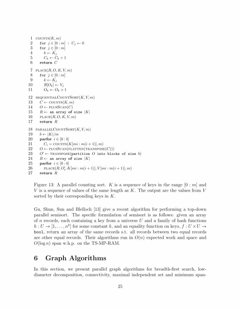
[0 : m]. The sort is given by parallelCountSort in Figure ??. It is similar to thesequential version, but works by breaking the input into blocks of size b = n/m. Eachblock does its own count of its keys. We then need to calculate the offset in the outputfor each block and each key for where the results should be placed. Like the sequentialcase this involves a plusScan, but it is across all blocks and buckets. Finally giventhe offsets, we again work across the blocks in parallel to place each value in the correctposition.

To analyzing the costs we note that the functions counts and place are fullysequential. When called on m keys they both take O(m) work and span. Acrossthe |K|/m parallel calls to them this comes to adds to O(|K|) work and O(m) span.The cost of the plusScan, flattening, and transposing is O(|K|) work and O(log |K|)span, for a total of O(|K|) work and O(m + log |K|) span. For integers in the range[0 : log |K|] this is great, with linear work and logarithmic span. However for a range[0 : n], it is completely sequential with O(n) work and span.

To uses this parallel counting sort in a radix sort on n integers, we use subkeysin the range [0 : nα], 0 < α ≤ 1. This leads to O(n) work and O(nα) span per callto counting sort. For integers in the range [0 : nc] there will be c/α calls to countingsort for a total of O(n/α) work, and O((nα + log n)/α) ⊂ O(nα/α) span, assuming cis constant.

For integers [0 : n logk n)] the best existing work-efficient integer sorting algorithmcan unstably sort integers in O(kn) work in expectation and O(k log n) span with highprobability [18]. However, since it is unstable it cannot be used in a radix sort.

5.5 Semisort

Given an array of keys and associated records, the semisorting problem is to compute areordered array where records with identical keys are contiguous. Unlike the output ofa sorting algorithm, records with distinct keys are not required to be in sorted order.Semisorting is a widely useful parallel primitive, and can be used to implement theshuffle-step in MapReduce, compute relational joins and efficiently implement parallelgraph algorithms that dynamically store frontiers in buckets, to give a few applications.

24

1 counts(K,m)2 for j ∈ [0 : m] : Cj ← 03 for j ∈ [0 : m]4 k ← Kj

5 Ck ← Ck + 16 return C

7 place(R,O,K, V,m)8 for j ∈ [0 : m]9 k ← Kj

10 R[Ok]← Vj11 Ok ← Ok + 1

12 sequentialCountSort(K,V,m)13 C ← counts(K,m)14 O ← plusScan(C)15 R← an array of size |K|16 place(R,O,K, V,m)17 return R

18 parallelCountSort(K,V,m)19 b← |K|/m20 parfor i ∈ [0 : b]21 Ci = counts(K[mi : m(i+ 1)],m)22 O ← plusScan(flatten(transpose(C)))23 O′ ← transpose(partition O into blocks of size b)24 R← an array of size |K|25 parfor i ∈ [0 : b]26 place(R,O′

i,K[mi : m(i+ 1)], V [mi : m(i+ 1)],m)27 return R

Figure 13: A parallel counting sort. K is a sequence of keys in the range [0 : m] andV is a sequence of values of the same length as K. The output are the values from Vsorted by their corresponding keys in K.

Gu, Shun, Sun and Blelloch [13] give a recent algorithm for performing a top-downparallel semisort. The specific formulation of semisort is as follows: given an arrayof n records, each containing a key from a universe U and a family of hash functionsh : U → [1, . . . , nk] for some constant k, and an equality function on keys, f : U ×U →bool, return an array of the same records s.t. all records between two equal recordsare other equal records. Their algorithms run in O(n) expected work and space andO(log n) span w.h.p. on the TS-MP-RAM.

6 Graph Algorithms

In this section, we present parallel graph algorithms for breadth-first search, low-diameter decomposition, connectivity, maximal independent set and minimum span-

25

edgeMap(G,U, fu) =parfor i ∈ [0 : |U |]N [i]← v ∈ N+(G, v) | fu(u, v)

return flatten(N)

Figure 14: edgeMap.

ning tree which illustrate useful techniques in parallel algorithms such as random-ization, pointer-jumping, and contraction. Unless otherwise specified, all graphs areassumed to be directed and unweighted. We use deg−(u) and deg+(u) to denote the inand out-degree of a vertex u for directed graphs, and deg(u) to denote the degree forundirected graphs.

6.1 Graph primitives

Many of our algorithms map over the edges incident to a subset of vertices, and returnneighbors that satisfy some predicate. Instead of repeatedly writing code perform-ing this operation, we express it using an operation called edgeMap in the style ofLigra [21].

edgeMap takes as input U , a subset of vertices and update, an update func-tion and returns an array containing all vertices v ∈ V s.t. (u, v) ∈ E, u ∈ U andupdate(u, v) = true. We will usually ensure that the output of edgeMap is a setby ensuring that a vertex v ∈ N(U) is atomically acquired by only one vertex in U .We give a simple implementation for edgeMap based on flatten in Figure 14. Thecode processes all u ∈ U in parallel. For each u we filter its out-neighbors and storethe neighbors v s.t. update(u, v) = true in a sequence of sequences, nghs. We returna flat array by calling flatten on nghs. It is easy to check that the work of thisimplementation is O(|U |+

∑u∈U deg+(u)) and the depth is O(log n).

We note that the flatten-based implementation given here is probably not verypractical; several papers [6, 21] discuss theoretically efficient and practically efficientimplementations of edgeMap.

6.2 Parallel breadth-first search

One of the classic graph search algorithms is breadth-first search (BFS). Given a graphG(V,E) and a vertex v ∈ V , the BFS problem is to assign each vertex reachable fromv a parent s.t. the tree formed by all (u, parent[u]) edges is a valid BFS tree (i.e.any non-tree edge (u, v) ∈ E is either within the same level of the tree or betweenconsecutive levels). BFS can be computed sequentially in O(m) work [12].

We give pseudocode for a parallel algorithm for BFS which runs in O(m) work andO(diam(G) log n) depth on the TS-MP-RAM in Figure 15. The algorithm first createsan initial frontier which just consists of v, initializes a visited array to all 0, and aparents array to all −1 and marks v as visited. We perform a BFS by looping while

26

BFS(G(V,E), v) =F ← v;parfor v ∈ V :

Xv ← false

Pv ← vXv ← true

while (|F | > 0)F ← edgeMap(G,F, λ(u, v).

if (testAndSet(Xv))Pv ← u;return true

return false

return P

Figure 15: Parallel breadth-first search.

the frontier is not empty and applying edgeMap on each iteration to compute thenext frontier. The update function supplied to edgeMap checks whether a neighborv is not yet visited, and if not applies a test-and-set. If the test-and-set succeeds, thenwe know that u is the unique vertex in the current frontier that acquired v, and so weset u to be the parent of v and return true, and otherwise return false.

6.3 Low-diameter decomposition

Many useful problems, like connectivity and spanning forest can be solved sequentiallyusing breadth-first search. Unfortunately, it is currently not known how to efficientlyconstruct a breadth-first search tree rooted at a vertex in polylog(n) depth on generalgraphs. Instead of searching a graph from a single vertex, like BFS, a low-diameterdecomposition (LDD) breaks up the graph into some number of connected clusters s.t.few edges are cut, and the internal diameters of each cluster are bounded (each clustercan be explored efficiently in parallel). Unlike BFS, low-diameter decompositions canbe computed efficiently in parallel, and lead to simple algorithms for a number of othergraph problems like connectivity, spanners, hop-sets, and low stretch spanning trees.

A (β, d)-decomposition partitions V into clusters, V1, . . . , Vk s.t. the shortest pathbetween two vertices in Vi using only vertices in Vi is at most d (strong diameter) andthe number of edges (u, v) where u ∈ Vi, v ∈ Vj, j 6= i is at most βm. Low-diameterdecompositions (LDD) were first introduced in the context of distributed computing [4],and were later used in metric embedding, linear-system solvers, and parallel algorithms.

Sequentially, LDDs can be found using a simple sequential ball-growing technique [4].The algorithm repeatedly picks an arbitrary uncovered vertex v and grows a ball aroundit using BFS until the number of edges incident to the current frontier is at most aβ fraction of the number of internal edges. It then removes the ball. Because of thestopping condition at most a β fraction of the edges will leave a ball. Also since eachlevel of the BFS will grow the number of edges by a factor of 1 + β, the number of

27

levels of the BFS is bounded by O(log(1+β)m) = O(log n/β). Therefore the algorithmgives a (β,O(log n/β)-decomposition. As each edge is examined once, the algorithmdoes O(n + m) work, but since the balls are visited one by one, in the worst case thealgorithm is fully sequential.

We will now discuss a work-efficient parallel algorithm [16]. As with the sequentialalgorithm it involves growing balls around vertices, but in this case in parallel. Startingto grow them all at the same time does not work since it would make every vertex itsown cluster. Instead the algorithm grows the balls from vertices based on start timesthat are randomly shifted based on the exponential distribution. The balls grow at therate of one level (edge) per unit time, and each vertex is assigned to the first ball thathits it. As in the sequential case, we can grow the balls using BFS.

Recall that a non-negative continuous random variable X has an exponential dis-tribution with rate parameter β > 0 if

Pr[X = x] = λe−βx .

By integration, the cumulative probability is:

Pr[X ≤ x] = 1− e−βx .

An important property of the exponential distribution is that it is memoryless, i.e.,

Pr[X > a+ | X > a] = Pr[X > b]

In words this says that if we take the tail of the distribution past a point a, andscale it so the the total remaining probability is 1 (i.e., conditioned on X > a), thenthe remaining distribution is the same as the original (it has forgotten that anythinghappened).

To select the start times each vertex v selects δv from an exponential distributionwith parameter β, and then each uses a start time Tv = δmax − δv, where δmax =maxv∈V δv. Note that the exponential distribution is subtracted, so the start timeshave a backwards exponential distribution, increasing instead of decreasing over time.In particular very few vertices will start in the first unit of time (often just one), andan exponentially growing number will start on each later unit of time. Based on thesestart times the first ball that hits a vertex u, and hence will be the cluster u is assignedto, is

Cu = arg minv∈V

(Tv + d(u, v))

This algorithm can be implemented efficiently using simultaneous parallel breadth-first searches. The initial breadth-first search starts at the vertex with the largest starttime, δmax. Each v ∈ V “wakes up” and starts its BFS if bTvc steps have elapsedand it is not yet covered by another vertex’s BFS. Figure 16 gives pseudocode for thealgorithm. The clusters assignment for each vertex, Cv, is initially set to unvisited, and

28

1 parfor v ∈ V : δv ← Exp(β);2 δmax = maxv∈V δv;3 parfor v ∈ V :

4 Tv ← δmax − δv;5 Cv ← unvisited;

6 γv ←∞7 l← 0;8 r ← 1;9 while (l < |V |)

10 F ← F ∪ v ∈ V | (Tv < r) ∧ (Cv = unvisited);11 l← l + |F |;12 edgeMap(G,F, λ(u, v).13 if (Cv = unvisited)14 c← Cu;

15 writeMin(γv, Tc − bTcc))16 F ← edgeMap(G,F, λ(u, v).17 c← Cu;

18 if (γv = Tc − bTcc)19 Cv ← c;20 return true

21 return false)22 r ← r + 123 return C

Figure 16: Low-diameter decomposition.

once set by the first arriving ball, it does not change. The γv variables are where theballs compete to see which has the earliest Tv—we only need the fractional part of Tvsince only those that arrive on the same round compete. A simpler implementation isto arbitrarily take one of the balls that arrive on the first round on which any arrive.It turns out this maintains the desired properties within a constant factor [22].

To analyze the work and span of the algorithm, we note the number of rounds ofthe algorithm is bounded by dδmaxe since every vertex will have been processed bythen. Line 10 can be implemented efficiently by pre-sorting the vertices by the roundthey start on, just pulling from the appropriate bucket on each round. A countingsort can be used giving linear work and O(log |V |+ δmax) span. Every vertex is in thefrontier at most once, and hence every edge is visited at most once, so the total workis O(|V | + |E|). Each round of the the algorithm has span at most O(log |V |), so thetotal span is O(δmax log |V |).

We now analyze the radius of clusters and number of edges between them. Wefirst argue that the maximum radius of each ball is O(log n/β) w.h.p. We alreadymentioned that the number of rounds of the LDD algorithm is bounded by δmax. Thisalso bounds the radius of any BFS and therefore the diameter is bounded by 2δmax.To bound δmax, consider the probability that a single vertex picks a shift larger than

29

c lognβ

:

Pr

[δv >

c log n

β

]= 1−Pr

[δv ≤

c log n

β

]= 1− (1− e−c logn) =

1

nc

Now, taking the union bound over all n vertices, we have that the probability of anyvertex picking a shift larger than c logn

βis:

Pr

[δmax >

c log n

β

]≤ 1

nc−1

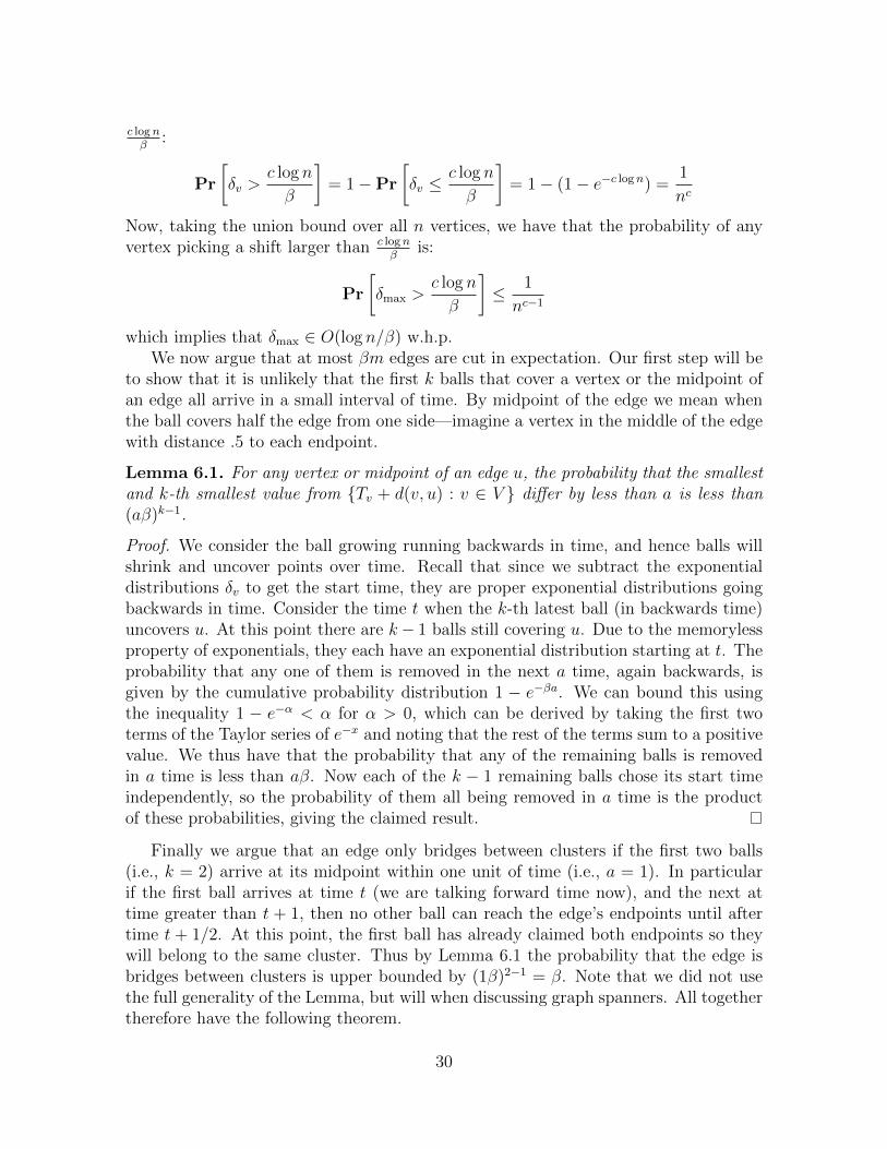
which implies that δmax ∈ O(log n/β) w.h.p.We now argue that at most βm edges are cut in expectation. Our first step will be

to show that it is unlikely that the first k balls that cover a vertex or the midpoint ofan edge all arrive in a small interval of time. By midpoint of the edge we mean whenthe ball covers half the edge from one side—imagine a vertex in the middle of the edgewith distance .5 to each endpoint.

Lemma 6.1. For any vertex or midpoint of an edge u, the probability that the smallestand k-th smallest value from Tv + d(v, u) : v ∈ V differ by less than a is less than(aβ)k−1.

Proof. We consider the ball growing running backwards in time, and hence balls willshrink and uncover points over time. Recall that since we subtract the exponentialdistributions δv to get the start time, they are proper exponential distributions goingbackwards in time. Consider the time t when the k-th latest ball (in backwards time)uncovers u. At this point there are k− 1 balls still covering u. Due to the memorylessproperty of exponentials, they each have an exponential distribution starting at t. Theprobability that any one of them is removed in the next a time, again backwards, isgiven by the cumulative probability distribution 1 − e−βa. We can bound this usingthe inequality 1 − e−α < α for α > 0, which can be derived by taking the first twoterms of the Taylor series of e−x and noting that the rest of the terms sum to a positivevalue. We thus have that the probability that any of the remaining balls is removedin a time is less than aβ. Now each of the k − 1 remaining balls chose its start timeindependently, so the probability of them all being removed in a time is the productof these probabilities, giving the claimed result.

Finally we argue that an edge only bridges between clusters if the first two balls(i.e., k = 2) arrive at its midpoint within one unit of time (i.e., a = 1). In particularif the first ball arrives at time t (we are talking forward time now), and the next attime greater than t + 1, then no other ball can reach the edge’s endpoints until aftertime t + 1/2. At this point, the first ball has already claimed both endpoints so theywill belong to the same cluster. Thus by Lemma 6.1 the probability that the edge isbridges between clusters is upper bounded by (1β)2−1 = β. Note that we did not usethe full generality of the Lemma, but will when discussing graph spanners. All togethertherefore have the following theorem.

30

Connectivity(G(V,E), β) =L← LDD(G, β);G′(V ′, E′) = Contract(G,L);if (|E′| = 0)

return LL′ ← Connectivity(G′, β)parfor v ∈ V :

u← Lv;

L′′v ← L′

u

return L’’

Figure 17: Parallel connectivity.

Theorem 6.1. For an undirected graph G = (V,E) and for for any β > 0 there is a

randomized parallel algorithm for finding a(β,O

(log |V |β

))-decomposition of the graph

in O(|V |+ |E|) work, and O(

log2 |V |β

)span.

Proof. We just showed that the probability that an edge goes between clusters is atmost β. By linearity of expectation across edges this means the expected number ofedges between components is at most β|E|. We showed above that δmax and hence the

diameter of the components are bounded by O(

log |V |β

)w.h.p.. Plugging δmax into the

cost analysis of the LDD algorithm gives the work and span bounds.

6.4 Connectivity

6.5 Spanners

A subgraph H of G = (V,E) is a k-spanner of G if for all paris of vertices u, v ∈ V ,dH(u, v) ≤ kdG(u, v). In particular the the spanner preserves distances within a factorof k. There a conjectured lower-bound that states that in general a spanner H musthave Ω(n1+1/dk/2e) edges [?]. The lower bound is based on the Erdos Girth Conjecture.The girth of a graph is the size of its smallest cycle, and the conjecture states thatthe maximum number of possible edges in a graph of girth k is Ω(n1+1/dk/2e). Anunweighted graph of with smallest cycle > k+ 1 cannot have a k-spanner since cuttingany edge would distort the weight on it cycles by a factor greater than k. Thereforethe girth conjecture, if true, implies the lower bound.

There are many sequential and parallel that achieve O(k)-spanners with O(n1+1/k)edges, with various tradeoffs [?]. Here we describe a simple parallel algorithm that useslow-diameter-decomposition (LDD). We first describe a variant for unweighted graphsand then outline how it can be used for the weighted case by bucketing the edges byweight.

31

N(G, v), N−(G, v), N+(G, v) neighbors of v in G (+ = out, − = in)N(G, V ), N−(G, V ), N+(G, V ) N(G, V ) =

⋃v∈V N(G, v) (similarly for N− and N+)

Figure 18: Some notation we use for graphs.

LubyMIS(G = (V,E)) =if (|V | = 0) return parfor v ∈ V : ρv ← random priority

I ← v ∈ V | ρ(v) < minu∈N(G,v) ρ(u)V ′ ← V \ (I ∪N(G, I))G′ ← (V ′, (u, v) ∈ E | (u ∈ V ′ ∧ v ∈ V ′))R← LubyMIS(G′)return I ∪R

Figure 19: Luby’s algorithm for MIS.

6.6 Maximal Independent Set

In a graph G = (V,E) we say a set of vertices U ⊂ V is an independent set if none ofthem are neighbors in G (i.e., (U ×U)∩E = ∅). A set of vertices U ⊂ V is a maximalindependent set (MIS) if it is an independent set and no vertex in V \U can be addedto U such that the result is an independent set. The MIS problem is to find an MISin a graph. Sequentially it is quite easy. Just put the vertices in arbitrary order, andthen add them one by one, such that whenever a vertex is added we remove all itsneighbors from consideration. This is a seemingly sequential process.

Here we describe Luby’s algorithm for finding an MIS efficiently in parallel. Pseu-docode is given in Figure 20. The algorithm works in a sequence of recursive calls.On each call in parallel it assigns the remaining vertices a random priority. Then itidentifies the set of vertices I that are a local maximum with respect to the priority(i.e. all of their neighbors have lower priorities). The set I is an independent set sinceno two neighbors can both be a local maximum, so the algorithm will add it to itsresult (the last line). However, it is not necessarily a maximal independent set. Toidentify more vertices to add to the MIS we remove the vertices I and their neighborsfrom the graph, along with their incident edges. We know the the neighbors N(G, I)cannot be in an independent set with I. Now the algorithms recurses on the remaininggraph.

We can argue the algorithm generates an MIS by induction. Inductively assume itis true on the smaller recursive call. The base case is true since an empty graph has novertices to place in an MIS. For any other call we know I is independent, and we knowthat given I is in the MIS, then no vertices in N(G, I) can be. Any remaining vertexin V ′ is independent of I. Since by induction the recursive call returned an MIS, thereare no additional vertices we can add to R such that the set will still be independent,and there are also none from N(G, I), showing that I ∪R is independent and maximal.

Proving the overall cost bounds is a bit trickier. What we will show is that we

32

u v

x w

Figure 20: Example for the proof of bounds for Luby’s algorithm.

expect to remove at least half the edges in each round (each recursive call). The proofis interesting because when adding a vertex to the MIS we will not be counting theremoval of its edges, but rather the removal of some of the edges of its neighbors. Thepurpose of this approach is to avoid multiple counting. It turns out that the expectedfraction of vertices that are kept on a round might be larger than 1/2—the actualnumber depends on the particular graph.

Theorem 6.2. One round of Luby’s algorithm removes at least half the edges in ex-pectation.

Proof. Consider an edge (u, v). Let Au,v be the event that u has the largest priorityamong u, v, and all their neighbors. Since priorities are selected uniformly at random,to determine the probability of this event we just have to count the number of suchvertices, which gives:

Pr[Au,v] ≥1

d(u) + d(v)

It is an inequality since u and v might share neighbors. Figure 20 illustrates an examplewhere Pr[Au,v] = 1/(d(u) + d(v)) = 1/(4 + 3) = 1/7. When the event Au,v occurs, uwill necessarily be selected to be in the MIS, and all the edges incident on v will beremoved since v is a neighbor of u and will itself be removed. Therefore we expect toremove Pr[Au,v]d(v) neighbors of v due to the event Au,v. Note that the edges incidenton u will also be removed, but we are not going to count these—except for (u, v) sinceit is a neighbor of v.

Now note that when we have an event Au,v we cannot on the same round haveanother event Aw,v since that would imply that both ρ(u) > ρ(w) and ρ(w) > ρ(u),which is not possible. Therefore if we count the edges incident on v removed by Au,v,we will not double count them due to another simultaneous event Aw,v. However sincean edge has two endpoints, an edge can still be counted twice, once from each of itsendpoints. In Figure 20, for example, we could simultaneously have the events Au,vand Aw,x, which would each count the edge v, x in edges it removes.

Let Y be a random variable giving the number of edges we remove in expectation.We claim the following is an expression for the expectation of Y .

E[Y ] ≥ 1

2

∑(u,v)∈E

(Pr[Au,v]d(v) + Pr[Av,u]d(u))

33

We get this by adding up the contribution of removed edges for both directions of theedge (u, v) and accounting for the double counting when removing an edge from eachof its endpoints (i.e., the 1/2 factor). Each term of the sum is at least 1, giving a totalE[Y ] ≥ |E|/2, which is what we were aiming to prove.

Now we consider the overall cost. Setting the priorities, taking the minimum ofthe neighbors to determine I, and generating the new graph can all be done withO(|V | + |E|) work and O(log |V |) span. Hence one call to LubyMIS without therecursive call, uses O(|V |+ |E|) work and O(log |V |) span. Intuitively since the numberof edges goes down by at least 1/2 in expectation, and a vertex will be removed if ithas no incident edges, the size of the graph will decrease geometrically. This wouldgive O(|V |+ |E|) work, O(log |E|) rounds and hence O(log2 |V |) span. However sinceit is a random process we need to be more careful.

Let Fi be a random variable for the fraction removed on step i, and let Mi bethe number of edges remaining on step i, i.e. Mi = mΠi−1

0 Fi. Lets say that we havethat E[Fi] ≤ β (for Luby’s algorithm β = 1/2). Furthermore since we are selectingpriorities at random in each round, this inequality holds even if conditioned on alloutcomes of all previous recursive calls. Let E[Fi] = β be the upper bound on theconditioned expectation. Given that these upper bounds are independent of previousFi, we can take the product of these bounded expectations to bound the expectationof the product of the Fi, giving:

E[Mi] ≤ mi−1∏j=0

E[Fi] = mβi

If the work on one round i is cMi (assuming |Ei| ≥ |Vi|), then by linearity of expecta-tions we have:

E[W (m)] ≤∞∑i=0

cE[Mi] ≤ cm∞∑i=0

βi = O(m)

The work on the vertices is bounded by the work on the edges.To bound the span we use Markov’s inequality:

Pr[X ≥ a] ≤ E[X]

a

and consider the probability Pr[Mi ≥ 1]. Note that if Mi < 1 then the algorithmfinishes since there are no edges left. So we just want to show that for sufficiently largei the probability is small. We have that:

Pr[Mi ≥ 1] ≤ E[Mi]

1≤ mβi

Setting i = k lgm for some k, we have:

34

Pr[Mi ≥ 1] ≤ mβk lgm = mmk lg β = m1+k log β

In our case β = 1/2, so lg β = −1, giving :

Pr[rounds < k lgm] ≥ 1−m1−k

This implies that the number of rounds is O(logm) (and hence also O(log n)) w.h.p.

7 Parallel Binary Trees

In this section, we present some parallel algorithms for balanced binary trees. Themethodology in this section is based on an algorithmic framework called join-basedalgorithms [7]. join is a primitive defined for each balancing scheme. All the other treealgorithms deal with rebalancing and rotations through join, and thus can be genericin code across multiple balancing schemes.

The function join(TL, e, TR) for a given balancing scheme takes two balanced binarytrees TL, TR balanced by that balancing scheme, and a single entry e as inputs, andreturns a new valid balanced binary tree, that has the same entries and the samein-order traversal as node(TL, e, TR), but satisfies the balancing criteria. We call themiddle entry e the pivot of the join.

7.1 Preliminaries

A binary tree is either a nil-node, or a node consisting of a left binary tree Tl, an entrye, and a right binary tree Tr, and denoted node(Tl, e, Tr). The entry can be simplya key, or a key-value pair. The size of a binary tree, or |T |, is 0 for a nil-node and|Tl| + |Tr| + 1 for a node(Tl, e, Tr). The weight of a binary tree, or w(T ), is one morethan its size (i.e., the number of leaves in the tree). The height of a binary tree, orh(T ), is 0 for a nil-node, and max(h(Tl), h(Tr)) + 1 for a node(Tl, e, Tr). Parent, child,ancestor and descendant are defined as usual (ancestor and descendant are inclusive ofthe node itself). A node is called a leaf when its both children are nil-nodes . The leftspine of a binary tree is the path of nodes from the root to a leaf always following theleft tree, and the right spine the path to a leaf following the right tree. The in-ordervalues (also referred to as the symmetric order) of a binary tree is the sequence ofvalues returned by an in-order traversal of the tree. When the context is clear, we usea node u to refer to the subtree Tu rooted at u, and vice versa.

A balancing scheme for binary trees is an invariant (or set of invariants) that is truefor every node of a tree, and is for the purpose of keeping the tree nearly balanced. Inthis section we consider four balancing schemes that ensure the height of every tree ofsize n is bounded by O(log n).

AVL Trees [3]. AVL trees have the invariant that for every node(Tl, e, Tr), the heightof Tl and Tr differ by at most one. This property implies that any AVL tree of size nhas height at most logφ(n+ 1), where φ = 1+

√5

2is the golden ratio.

35

Notation Description|T | The size of tree Th(T ) The height of tree T

h(T ) The black height of an RB tree Tw(T ) The weight of tree T (i.e, |T |+ 1)p(T ) The parent of node Tk(T ) The key of node Tlc(T ) The left child of node Trc(T ) The right child of node T

expose(T ) 〈lc(T ), k(T ), rc(T )〉

Table 2: Summary of notation.

Red-black (RB) Trees [5].. RB trees associate a color with every node and maintaintwo invariants: (the red rule) no red node has a red child, and (the black rule) thenumber of black nodes on every path from the root down to a leaf is equal. All nil-nodes are always black. Unlike some other presentations, we do not require that theroot of a tree is black. Although this does not affect the correctness of our algorithms,our proof of the work bounds requires allowing a red root. We define the black heightof a node T , denoted h(T ) to be the number of black nodes on a downward path fromthe node to a leaf (inclusive of the node). Any RB tree of size n has height at most2 log2(n+ 1).

Weight-balanced (WB) Trees. WB trees are defined with parameter α (also called

BB[α] trees) [17] maintain for every T = node(Tl, e, Tr) the invariant α ≤ w(Tl)w(T )

≤ 1−α.

We say two weight-balanced trees T1 and T2 have like weights if node(T1, e, T2) is weightbalanced. Any α weight-balanced tree of size n has height at most log 1

1−αn. For

211< α ≤ 1− 1√

2insertion and deletion can be implemented on weight balanced trees

using just single and double rotations [17, ?]. We require the same condition for ourimplementation of join, and in particular use α = 0.29 in experiments. We also denoteβ = 1−α

α, which means that either subtree could not have a size of more than β times

of the other subtree.

Treaps. [19] Treaps associate a uniformly random priority with every node and main-tain the invariant that the priority at each node is no greater than the priority of itstwo children. Any treap of size n has height O(log n) with high probability (w.h.p).

The notation we use for binary trees is summarized in Figure 2.

7.2 The join Algorithms for Each Balancing Scheme

Here we describe algorithms for join for the four balancing schemes we defined inChapter 7.1, as well as define the rank for each of them. We will then prove they arejoinable. For join, the pivot can be either just the data entry (such that the algorithmwill create a new tree node for it), or a pre-allocated tree node in memory carrying

36

the corresponding data entry (such that the node may be reused, allowing for in-placeupdates).

As mentioned in the introduction and the beginning of this chapter, join fullycaptures what is required to rebalance a tree and can be used as the only function thatknows about and maintains the balance invariants. For AVL, RB and WB trees weshow that join takes work that is proportional to the difference in rank of the two trees.For treaps the work depends on the priority of k. All the join algorithms are sequentialso the span is equal to the work. We show in this thesis that the join algorithms forall balancing schemes we consider lead to optimal work for many functions on mapsand sets.

7.2.1 AVL Trees

1 joinRightAVL(Tl, k, Tr)

2 (l, k′, c) = expose(Tl);3 if h(c) ≤ h(Tr) + 1 then

4 T ′ = node(c, k, Tr);5 if h(T ′) ≤ h(l) + 1 then return node(l, k′, T ′);6 else return rotateLeft(node(l, k′, rotateRight(T ′)));7 else

8 T ′ = joinRightAVL(c, k, Tr);9 T ′′ = node(l, k′, T ′);10 if h(T ′) ≤ h(l) + 1 then return T ′′; else return rotateLeft(T ′′);

11 join(Tl, k, Tr)

12 if h(Tl) > h(Tr) + 1 then return joinRightAVL(Tl, k, Tr);13 else if h(Tr) > h(Tl) + 1 then return joinLeftAVL(Tl, k, Tr);14 else return node(Tl, k, Tr);

Figure 21: The join algorithm on AVL trees – joinLeftAVL is symmetric tojoinRightAVL.

For AVL trees, we define the rank as the height, i.e., r(T ) = h(T ). Pseudocodefor AVL join is given in Figure 21 and illustrated in Figure 22. Every node storesits own height so that h(·) takes constant time. If the two trees Tl and Tr differ byheight at most one, join can simply create a new node(Tl, e, Tr). However if they differby more than one then rebalancing is required. Suppose that h(Tl) > h(Tr) + 1 (theother case is symmetric). The idea is to follow the right spine of Tl until a node c forwhich h(c) ≤ h(Tr) + 1 is found (line 3). At this point a new node(c, e, Tr) is created toreplace c (line 4). Since either h(c) = h(Tr) or h(c) = h(Tr) + 1, the new node satisfiesthe AVL invariant, and its height is one greater than c. The increase in height canincrease the height of its ancestors, possibly invalidating the AVL invariant of thosenodes. This can be fixed either with a double rotation if invalid at the parent (line 6)or a single left rotation if invalid higher in the tree (line 10), in both cases restoring

37

the height for any further ancestor nodes. The algorithm will therefore require at mosttwo rotations, as we summarized in the following lemma.

Lemma 7.1. The join algorithm in Figure 21 on AVL trees requires at most tworotations.

Step 1: connect Step 2: rebalance

k

𝑇𝑇𝑅𝑅

(h)

p

a c

The right branch in 𝑇𝑇𝐿𝐿 𝑇𝑇𝑅𝑅 𝑘𝑘

……

d

h+2 Rebalance required if ℎ 𝑇𝑇1 = ℎ

ℎ 𝑇𝑇2 = ℎ + 1

h+2

𝑇𝑇1

(h)

c

p

a c1

……

𝐿𝐿 𝑇𝑇2 (h or h-1)

𝑇𝑇𝑅𝑅

(h)

k

c2 d

𝑅𝑅 𝑇𝑇2 (h or h-1)

𝑇𝑇1

(h or h+1)

𝑇𝑇𝑅𝑅

(h)

k

p

a

c d

……

𝑇𝑇2

(h or h+1)

𝑇𝑇1

(h or h+1)

𝑇𝑇2 (h or h+1)

Figure 22: An example for join on AVL trees – An example for join on AVLtrees (h(Tl) > h(Tr) + 1). We first follow the right spine of Tl until a subtree of heightat most h(Tr) + 1 is found (i.e., T2 rooted at c). Then a new node(c, k, Tr) is created,replacing c (Step 1). If h(T1) = h and h(T2) = h+ 1, the node p will no longer satisfythe AVL invariant. A double rotation (Step 2) restores both balance and its originalheight.

Lemma 7.2. For two AVL trees Tl and Tr, the AVL join algorithm works correctly,runs with O(|h(Tl)−h(Tr)|) work, and returns a tree satisfying the AVL invariant withheight at most 1 + max(h(Tl), h(Tr)).

Proof. Since the algorithm only visits nodes on the path from the root to c, and onlyrequires at most two rotations (Lemma 7.1), it does work proportional to the pathlength. The path length is no more than the difference in height of the two trees sincethe height of each consecutive node along the right spine of Tl differs by at least one.Along with the case when h(Tr) > h(Tl) + 1, which is symmetric, this gives the statedwork bounds. The resulting tree satisfies the AVL invariants since rotations are usedto restore the invariant. The height of any node can increase by at most one, so theheight of the whole tree can increase by at most one.

7.2.2 Red-black Trees

Tarjan describes how to implement the join function for red-black trees [?]. Herewe describe a variant that does not assume the roots are black (this is to bound theincrease in rank by union). The pseudocode is given in Figure 23. We store at everynode its black height h(·). Also, we define the increase-2 node as a black node, whoseboth children are also black. This means that the node increases the rank of its childrenby 2. In the algorithm, the first case is when h(Tr) = h(Tl). Then if the input nodeis a increase-2 node, we use it as a black node and directly concatenate the two inputtrees. This increases the rank of the input by at most 2. Otherwise, if both root(Tr)

38

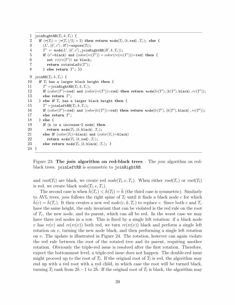
1 joinRightRB(Tl, k, Tr)

2 if (r(Tl) = br(Tr)/2c × 2) then return node(Tl, 〈k, red〉 , Tr); else

3 (L′, 〈k′, c′〉 , R′)=expose(Tl);4 T ′ = node(L′, 〈k′, c′〉,joinRightRB(R′, k, Tr));5 if (c′=black) and (color(rc(T ′)) = color(rc(rc(T ′)))=red) then

6 set rc(rc(T ′)) as black;

7 return rotateLeft(T ′);8 else return T ′;

9 joinRB(Tl, k, Tr)

10 if Tl has a larger black height then

11 T ′ =joinRightRB(Tl, k, Tr);12 if (color(T ′)=red) and (color(rc(T ′))=red) then return node(lc(T ′), 〈k(T ′), black〉 , rc(T ′));13 else return T ′;

14 else if Tr has a larger black height then

15 T ′ =joinLeftRB(Tl, k, Tr);16 if (color(T ′)=red) and (color(lc(T ′))=red) then return node(lc(T ′), 〈k(T ′), black〉 , rc(T ′));17 else return T ′;

18 else

19 if (k is a increase-2 node) then20 return node(Tl, 〈k, black〉 , Tr);21 else if (color(Tl)=black) and (color(Tr)=black)22 return node(Tl, 〈k, red〉 , Tr);23 else return node(Tl, 〈k, black〉 , Tr);

24

Figure 23: The join algorithm on red-black trees – The join algorithm on red-black trees. joinLeftRB is symmetric to joinRightRB.

and root(Tl) are black, we create red node(Tl, e, Tr). When either root(Tr) or root(Tl)is red, we create black node(Tl, e, Tr).

The second case is when h(Tr) < h(Tl) = h (the third case is symmetric). Similarlyto AVL trees, join follows the right spine of Tl until it finds a black node c for whichh(c) = h(Tr). It then creates a new red node(c, k, Tr) to replace c. Since both c and Trhave the same height, the only invariant that can be violated is the red rule on the rootof Tr, the new node, and its parent, which can all be red. In the worst case we mayhave three red nodes in a row. This is fixed by a single left rotation: if a black nodev has rc(v) and rc(rc(v)) both red, we turn rc(rc(v)) black and perform a single leftrotation on v, turning the new node black, and then performing a single left rotationon v. The update is illustrated in Figure 24. The rotation, however can again violatethe red rule between the root of the rotated tree and its parent, requiring anotherrotation. Obviously the triple-red issue is resolved after the first rotation. Therefore,expect the bottommost level, a triple-red issue does not happen. The double-red issuemight proceed up to the root of Tl. If the original root of Tl is red, the algorithm mayend up with a red root with a red child, in which case the root will be turned black,turning Tl rank from 2h−1 to 2h. If the original root of Tl is black, the algorithm may

39

end up with a red root with two black children, turning the rank of Tl from 2h− 2 to2h− 1. In both cases the rank of the result tree is at most 1 + r(Tl).

We note that the rank of the output can increase the larger rank of the input treesby 2 only when the pivot is an increase-2 node and the two input trees are balancedboth with black roots. In general we do not need to deal with the increase-2 nodesspecifically for a correct join algorithm. We define the increasing-2 nodes for thepurpose of bounding the cost of some join-based algorithms.

Lemma 7.3. For two RB trees Tl and Tr, the RB join algorithm works correctly, runswith O(|h(Tl)− h(Tr)|) work, and returns a tree satisfying the red-black invariants andwith black height at most 1 + max(h(Tl), h(Tr)).

Proof. The base case where h(Tl) = h(Tr) is straight-forward. For symmetry, here weonly prove the case when h(Tl) > h(Tr). We prove the proposition by induction.

We first show the correctness. As shown in Figure 24, after appending Tr to Tl, if pis black, the rebalance has been done, the height of each node stays unchanged. Thusthe RB tree is still valid. Otherwise, p is red, p’s parent g must be black. By applyinga left rotation on p and g, we get a balanced RB tree rooted at p, except the root pis red. If p is the root of the whole tree, we change p’s color to black, and the heightof the whole tree increases by 1. The RB tree is still valid. Otherwise, if the currentparent of p (originally g’s parent) is black, the rebalance is done here. Otherwise asimilar rebalance is required on p and its current parent. Thus finally we will eitherfind the current node valid (current red node has a black parent), or reach the root,and change the color of root to be black. Thus when we stop, we will always get avalid RB tree.

Since the algorithm only visits nodes on the path from the root to c, and onlyrequires at most a single rotation per node on the path, the overall work for thealgorithm is proportional to the depth of c in Tr. This in turn is no more than twicethe difference in black height of the two trees since the black height decrements at leastevery two nodes along the path. This gives the stated work bounds.

For the rank, note that throughout the algorithm, before reaching the root, the blackrule is never invalidated (or is fixed immediately), and the only invalidation occurs onthe red rule. If the two input trees are originally balanced, the rank increases by atmost 2. The only case that the rank increases by 2 is when k is from an increase-2node, and both root(Tr) and root(Tl) are black.

If the two input tree are not balanced, the black height of the root does not changebefore the algorithm reaching the root (Step 3 in Figure 24). There are then threecases:

1. The rotation does not propagate to the root, and thus the rank of the tree remainsas max(h(Tl), h(Tr)).

2. (Step 3 Case 1) The original root color is red, and thus a double-red issue occursat the root and its right child. In this case the root is colored black. The black

40

height of the tree increases by 1, but since the original root is red, the rankincreases by only 1.

3. (Step 3 Case 1) The original root color is black, but the double-red issue occursat the root’s child and grandchild. In this case another rotation is applied asshown in Figure 24. The black height remains, but the root changed from blackto red, increasing the rank by 1.

𝑇𝑇1

(h)

𝑇𝑇2

(h)

𝑇𝑇3

(h)

𝑇𝑇𝑅𝑅

(h)

p

g

a b c d

k

……

Step 1: connect (when 𝑝𝑝 is red)

Step 2: rebalance (when 𝑝𝑝 is red)

Red node Black node Node of either color

k

𝑇𝑇𝑅𝑅

(h)

𝑇𝑇1

(h) 𝑇𝑇2

(h) 𝑇𝑇3

(h)

p

g

a

b c

The right branch in 𝑇𝑇𝐿𝐿 𝑇𝑇𝑅𝑅 𝑘𝑘 ……

d

𝑇𝑇1

(h) 𝑇𝑇2

(h) 𝑇𝑇3

(h)

𝑇𝑇𝑅𝑅

(h)

p

g

k a

b

c

……

d

Rebalance required on: 𝒈𝒈: 𝑝𝑝 and 𝑘𝑘 are red 𝒑𝒑: 𝑘𝑘 and 𝑑𝑑 are red, 𝑝𝑝 is black

Step 3: adjust on root

r v

r v

1) When k(𝑇𝑇𝐿𝐿) is red, after rotation on 𝐿𝐿(𝑇𝑇𝐿𝐿):

2) When k(𝑇𝑇𝐿𝐿) is black, after rotation on 𝑘𝑘(𝑇𝑇𝐿𝐿):

v

u

If the unbalance propagate to the root of 𝑇𝑇𝐿𝐿:

r

Rank increases from 2ℎ + 1 to 2(ℎ + 1)

Rank increases from 2ℎ to 2ℎ + 1

r v

u w

Figure 24: An example of join on red-black trees – An example of join on red-black trees (h = h(Tl) > h(Tr)). We follow the right spine of Tl until we find a blacknode with the same black height as Tr (i.e., c). Then a new red node(c, k, Tr) is created,replacing c (Step 1). The only invariant that can be violated is when either c’s previousparent p or Tr’s root d is red. If so, a left rotation is performed at some black node.Step 2 shows the rebalance when p is red. The black height of the rotated subtree (nowrooted at p) is the same as before (h+ 1), but the parent of p might be red, requiringanother rotation. If the red-rule violation propagates to the root, the root is eithercolored red, or rotated left (Step 3).

7.2.3 Weight Balanced Trees

For WB trees r(T ) = log2(w(T )) − 1. We store the weight of each subtree at everynode. The algorithm for joining two weight-balanced trees is similar to that of AVLtrees and RB trees. The pseudocode is shown in Figure 25. The like function in

41

1 joinRightWB(Tl, k, Tr)

2 (l, k′, c)=expose(Tl);3 if (balance(|Tl|, |Tr|) then return node(Tl, k, Tr)); else

4 T ′ = joinRightWB(c, k, Tr);5 (l1, k1, r1) = expose(T ′);6 if like(|l|, |T ′|) then return node(l, k′, T ′);7 else if (like(|l|, |l1|)) and (like(|l|+ |l1|, r1)) then return rotateLeft(node(l, k′, T ′));8 else return rotateLeft(node(l, k′,rotateRight(T ′)));

9 joinWB(Tl, k, Tr)

10 if heavy(Tl, Tr) then return joinRightWB(Tl, k, Tr);11 else if heavy(Tr, Tl) then return joinLeftWB(Tl, k, Tr);12 else return node(Tl, k, Tr);

Figure 25: The join algorithm on weight-balanced trees – joinLeftWB is sym-metric to joinRightWB.

the code returns true if the two input tree sizes are balanced based on the factor ofα, and false otherwise. If Tl and Tr have like weights the algorithm returns a newnode(Tl, e, Tr). Suppose |Tr| ≤ |Tl|, the algorithm follows the right branch of Tl untilit reaches a node c with like weight to Tr. It then creates a new node(c, r, Tr) replacingc. The new node will have weight greater than c and therefore could imbalance theweight of c’s ancestors. This can be fixed with a single or double rotation (as shownin Figure 26) at each node assuming α is within the bounds given in Section 7.1.

v

𝐷𝐷 𝐵𝐵

u

5 3

The right branch in 𝑇𝑇𝐿𝐿 ……

𝐶𝐶

2 4

𝐴𝐴

1

v

𝐷𝐷 𝐴𝐴 𝐶𝐶

u

1

4

(1). Single Rotation ……

3 5

𝐵𝐵

2

v

𝐶𝐶 𝐷𝐷 𝐵𝐵

u

3

(2). Double Rotation ……

𝐴𝐴

1 (0): The rebalance process is currently at 𝑣𝑣, which means the tree rooted at 𝑢𝑢 and all of its subtrees are balanced. (1): The result of the single rotation. (2): The result of the double rotation.

(0)

2 5 4

Figure 26: An illustration of single and double rotations possibly needed torebalance weight-balanced trees – In the figure the subtree rooted at u has becomeheavier due to joining in Tl and its parent v now violates the balance invariant.

42

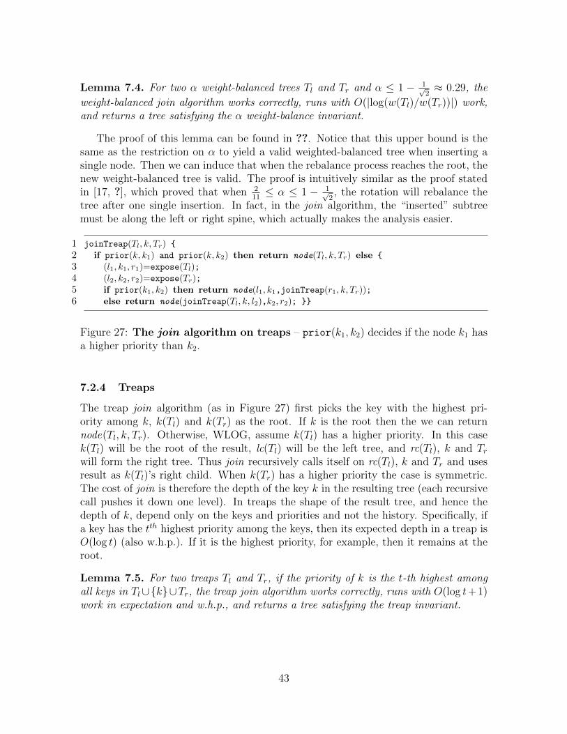
Lemma 7.4. For two α weight-balanced trees Tl and Tr and α ≤ 1 − 1√2≈ 0.29, the

weight-balanced join algorithm works correctly, runs with O(|log(w(Tl)/w(Tr))|) work,and returns a tree satisfying the α weight-balance invariant.

The proof of this lemma can be found in ??. Notice that this upper bound is thesame as the restriction on α to yield a valid weighted-balanced tree when inserting asingle node. Then we can induce that when the rebalance process reaches the root, thenew weight-balanced tree is valid. The proof is intuitively similar as the proof statedin [17, ?], which proved that when 2

11≤ α ≤ 1 − 1√

2, the rotation will rebalance the

tree after one single insertion. In fact, in the join algorithm, the “inserted” subtreemust be along the left or right spine, which actually makes the analysis easier.

1 joinTreap(Tl, k, Tr)

2 if prior(k, k1) and prior(k, k2) then return node(Tl, k, Tr) else

3 (l1, k1, r1)=expose(Tl);4 (l2, k2, r2)=expose(Tr);5 if prior(k1, k2) then return node(l1, k1,joinTreap(r1, k, Tr));6 else return node(joinTreap(Tl, k, l2),k2, r2);

Figure 27: The join algorithm on treaps – prior(k1, k2) decides if the node k1 hasa higher priority than k2.

7.2.4 Treaps

The treap join algorithm (as in Figure 27) first picks the key with the highest pri-ority among k, k(Tl) and k(Tr) as the root. If k is the root then the we can returnnode(Tl, k, Tr). Otherwise, WLOG, assume k(Tl) has a higher priority. In this casek(Tl) will be the root of the result, lc(Tl) will be the left tree, and rc(Tl), k and Trwill form the right tree. Thus join recursively calls itself on rc(Tl), k and Tr and usesresult as k(Tl)’s right child. When k(Tr) has a higher priority the case is symmetric.The cost of join is therefore the depth of the key k in the resulting tree (each recursivecall pushes it down one level). In treaps the shape of the result tree, and hence thedepth of k, depend only on the keys and priorities and not the history. Specifically, ifa key has the tth highest priority among the keys, then its expected depth in a treap isO(log t) (also w.h.p.). If it is the highest priority, for example, then it remains at theroot.

Lemma 7.5. For two treaps Tl and Tr, if the priority of k is the t-th highest amongall keys in Tl∪k∪Tr, the treap join algorithm works correctly, runs with O(log t+1)work in expectation and w.h.p., and returns a tree satisfying the treap invariant.

43

Function Work Spaninsert , delete, update, find , first , last ,

O(log n) O(log n)range, split , join2 , previous , next , rank ,select , up to, down tounion, intersection, difference O

(m log

(nm

+ 1))

O(log n logm)map, reduce, map reduce, to array O(n) O(log n)

build , filter O(n) O(log2 n)

Table 3: The core join-based algorithms and their asymptotic costs – Thecost is given under the assumption that all parameter functions take constant time toreturn. For functions with two input trees (union, intersection and difference), n isthe size of the larger input, and m of the smaller.

Split

1 split(T, k)

2 if T = ∅ then3 return (∅,false,∅);4 (L,m,R) = expose(T );5 if k = m then return (L,true,R);6 if k < m then

7 (TL, b, TR) = split(L, k);8 return (TL,b,join(TR,m,R));

9 (TL, b, TR) = split(R, k);10 return (join(L,m, TL), b, TR);

join2

1 split_last(T ) // split_first is symmetric

2 (L, k,R) = expose(T );3 if R = ∅ then return(L, k);4 (T ′, k′) = split_last(R);5 return (join(L, k, T ′),k′);

6 join2(Tl,Tr)

7 if Tl = ∅ then return Tr;8 (T ′, k) = split_last(Tl);9 return join(T ′, k, Tr);

10

Figure 28: split and join2 algorithms – They are both independent of balancingschemes.

7.3 Algorithms Using join

The join function, as a subroutine, has been used and studied by many researchers andprogrammers to implement more general set operations. In this section, we describealgorithms for various functions that use just join. The algorithms are generic acrossbalancing schemes. The pseudocodes for the algorithms in this section is shown inFigure 30. Beyond join the only access to the trees we make use of is through expose,which only read the root. main set operations, which are union, intersection anddifference, are optimal (or known as efficient) in work. The pseudocode for all thealgorithms introduced in this section is presented in Figure 31.

7.3.1 Two Helper Functions: split and join2

We start with presenting two helper functions split and join2 . For a BST T and keyk, split(T, k) returns a triple (Tl, b, Tr), where Tl (Tr) is a tree containing all keys in Tthat are less (larger) than k, and b is a flag indicating whether k ∈ T . join2 (Tl, Tr)

44

returns a binary tree for which the in-order values is the concatenation of the in-ordervalues of the binary trees Tl and Tr (the same as join but without the middle key).For BSTs, all keys in Tl have to be less than keys in Tr.

Although both sequential, these two functions, along with the join function, areessential for help other algorithms to achieve good parallelism. Intuitively, when pro-cessing a tree in parallel, we recurse on two sub-components of the tree in parallelby split ing the tree by some key. In many cases, the splitting key is just the root,which means directly using the two subtrees of natural binary tree structure. Afterthe recursions return, we combine the result of the left and right part, with or withoutthe middle key, using join or join2 . Because of the balance of the tree, this frameworkusually gives high parallelism with shallow span (e.g., poly-logarithmic).

Split.. As mentioned above, split(T, k) splits a tree T by a key k into Tl and Tr, alongwith a bit b indicating if k ∈ T . Intuitively, the split algorithm first searches for k in T ,splitting the tree along the path into three parts: keys to the left of the path, k itself (ifit exists), and keys to the right. Then by applying join, the algorithm merges all thesubtrees on the left side (using keys on the path as intermediate nodes) from bottom totop to form Tl, and merges the right parts to form Tr. Writing the code in a recursivemanner, this algorithm first determine if k falls in the left (right) subtree, or is exactlythe root. If it is the root, then the algorithm straightforwardly returns the left andthe right subtrees as the two return trees and true as the bit b. Otherwise, WLOG,suppose k falls in the left subtree. The algorithm further split the left subtree into TLand TR with the return bit b′. Then the return bit b = b′, the Tl in the final result willbe TL, and Tr means to join TR with the original right subtree by the original root.Figure 29 gives an example.

25

13

^

8

5 12

^ ^ ^ ^

17

15 22

^ ^ ^

51

^

36

30 42

^ ^ ^ ^

80

70 95

^ ^ ^

13

^

8

5 12

^ ^ ^ ^

17

15 22

^ ^ ^

^

30

^

^ 36 , , 𝑗𝑗𝑗𝑗𝑗𝑗𝑗𝑗( ) , 25 𝑇𝑇𝐿𝐿 = 𝑗𝑗𝑗𝑗𝑗𝑗𝑗𝑗( ) ,

^ 𝑇𝑇𝑅𝑅 = 𝑗𝑗𝑗𝑗𝑗𝑗𝑗𝑗( ) , 51

^

80

70 95

^ ^ ^

Split 𝑇𝑇 with key 42:

, 𝑏𝑏 = 𝑡𝑡𝑡𝑡𝑡𝑡𝑡𝑡

Figure 29: An example of split in a BST with key 42 – We first search for 42 inthe tree and split the tree by the searching path, then use join to combine trees on theleft and on the right respectively, bottom-top.

The cost of the algorithm is proportional to the rank of the tree, as we summarizeand prove in the following theorem.

Theorem 7.1. The work of split(T, k) is O(h(T )) for AVL, RB, WB trees and treaps.

Proof Sketch. We only consider the work of joining all subtrees on the left side. Theother side is symmetric. Suppose we have l subtrees on the left side, denoted from

45

bottom to top as T1, T2, . . . Tl. We consecutively join T1 and T2 returning T ′2, then joinT ′2 with T3 returning T ′3 and so forth, until all trees are merged. The overall work ofsplit is the sum of the cost of l − 1 join functions.

We now use an AVL tree as an example to show the proof. Recall that each joincosts time O(|h(Ti+1)−h(T ′i )|), and increase the height of Ti+1 by at most 1. Also h(T ′i )is achieved by joining Ti and T ′i−1. Considering Ti is a subtree in Ti+1’s sibling, and thus

h(T ′i ) is no more than h(Ti+1) + 2. The overall complexity is∑l

i=1 |h(Ti+1)− h(T ′i )| ≤∑li=1 h(Ti+1)− h(T ′i ) + 2 = O(h(T )).For RB and WB trees, the proof is similar to the above proof for AVL trees, but

only changes join cost based on the difference in black-height or log of weight, insteadof height.

For treaps, each join uses the key with the highest priority since the key is alwayson a upper level. Hence by Lemma 7.5, the complexity of each join is O(1) and thework of split is at most O(h(T )).

Join2.. As stated above, the join2 function is defined similar to join without themiddle entry. The join2 algorithm first choose one of the the input trees, and extract itslast (if it is Tl) or first (if it is Tr) element k. The two cases take the same asymptoticalcost. The extracting process is similar to the split algorithm. The algorithm then usesk as the pivot to join the two trees. In the code shown in Figure 28, the split lastalgorithm first finds the last element k (by following the right spine) in Tl and on theway back to root, joins the subtrees along the path. We denote the result of droppingk in TL as T ′. Then join(T ′, k, Tr) is the result of join2 . Unlike join, the work ofjoin2 is proportional to the rank of both trees since both split and join take at mostlogarithmic work.

Theorem 7.2. The work of T =join2(Tl, Tr) is O(r(Tl) + r(Tr)) for all joinable trees.

The cost bound holds because split last and join both take work asymptotically nomore than the larger tree rank.

7.4 Set-set Functions Using join

In this section, we will present the join-based algorithm on set-set functions, includingunion, intersection and difference. Many other set-set operations, such as symmetricdifference, can be implemented by a combination of union, intersection and differencewith no extra asymptotical work. We will start with presenting some background ofthese algorithms, and then explain in details about the join-based algorithms. Finally,we show the proof of their cost bound.

Background. The parallel set-set functions are particularly useful when using parallelmachines since they can support parallel bulk updates. As mentioned, although sup-porting efficient algorithms for basic operations on trees, such as insertion and deletion,are rather straightforward, implementing efficient bulk operations is more challenging,

46

Union

union(T1,T2)

if T1 = ∅ then return T2;if T2 = ∅ then return T1;(L2,k2,R2) = expose(T2);(L1,b,R1) = split(T1,k2);Tl = union(L1,L2) ‖

Tr = union(R1,R2);return join(Tl,k2,Tr);

Intersection

intersect(T1,T2)

if T1 = ∅ then return ∅;if T2 = ∅ then return ∅;(L2,k2,R2) = expose(T2);(L1,b,R1) = split(T1,k2);Tl = intersect(L1,L2) ‖Tr = intersect(R1,R2);

if b then return join(Tl,k2,Tr);else return join2(Tl,Tr);

Difference

difference(T1,T2)

if T1 = ∅ then ∅;if T2 = ∅ then T1;(L2,k2,R2) = expose(T2);(L1,b,R1) = split(T1,k2);Tl = difference(L1,L2) ‖Tr = difference(R1,R2);

return join2(Tl,Tr);

Figure 30: join-based algorithms for set-set operations – They are all indepen-dent of balancing schemes. The syntax S1||S2 means that the two statements S1 andS2 can be run in parallel based on any fork-join parallelism.

especially considering parallelism and different balancing schemes. For example, com-bining two ordered sets of size n and m ≤ n in the format of two arrays would takework O(m+n) using the standard merging algorithm in the merge sort algorithm. Thismakes even inserting an single element into a set of size n to have linear cost. This isbecause even most of the chunks of data in the input remain consecutive, the algorithmstill need to scan and copy them to the output array. Another simple implementationis to store both sets as balanced trees, and insert the elements in the smaller tree intothe larger one, costing O(m log n) work. It overcomes the issue of redundant scanningand copying, because many subtrees in the larger tree remain untouched. However,this results in O(n log n) time, for combining two ordered sets of the same size, whileit is easy to make it O(n) by arrays. The problem lies in that the algorithm fails tomake use of the ordering in the smaller tree.

The lower bound for comparison-based algorithms for union, intersection and dif-ference for inputs of size n and m ≤ n, and returning an ordered structure2, islog2

(m+nn

)= Θ

(m log

(nm

+ 1))

((m+nn

)is the number of possible ways n keys can

be interleaved with mkeys). The bound is interesting since it shows that implementinginsertion with union, or deletion with difference, is asymptotically efficient (O(log n)time), as is taking the union of two equal sized sets (O(n) time).

Brown and Tarjan first matched these bounds, asymptotically, using a sequentialalgorithm based on red-black trees [10]. Adams later described very elegant algorithmsfor union, intersection, and difference, as well as other functions based on join [1, 2].Adams’ algorithms were proposed in an international competition for the Standard MLcommunity, which is about implementations on “set of integers”. Prizes were awardedin two categories: fastest algorithm, and most elegant yet still efficient program. Adamswon the elegance award, while his algorithm is almost as fast as the fastest programfor very large sets, and was faster for smaller sets. Because of the elegance of the

2By “ordered structure” we mean any data structure that can output elements in sorted orderwithout any further comparisons—e.g., a sorted array, or a binary search tree.

47

algorithm, at least three libraries use Adams’ algorithms for their implementation ofordered sets and tables (Haskell [15] and MIT/GNU Scheme, and SML). Indeed thejoin-based algorithm that will be introduced later in this section is based on Adams’algorithms. Blelloch and Reid-Miller later show that similar algorithms for treaps [9],are optimal for work (i.e. Θ

(m log

(nm

+ 1))

), and are also parallel. Later, Blellochet al. [7] extend Adams’ algorithms to multiple balancing schemes and prove the costbound.

Algorithms. union(T1, T2) takes two BSTs and returns a BST that contains the unionof all keys. The algorithm uses a classic divide-and-conquer strategy, which is parallel.At each level of recursion, T1 is split by k(T2), breaking T1 into three parts: one withall keys smaller than k(T2) (denoted as L1), one in the middle either of only one keyequal to k(T2) (when k(T2) ∈ T1) or empty (when k(T2) /∈ T1), the third one with allkeys larger than k(T2) (denoted as R1). ger) than k(T1). Then two recursive calls tounion are made in parallel. One unions lc(T2) with L1, returning Tl, and the other oneunions rc(T2) with R1, returning Tr. Finally the algorithm returns join(Tl, k(T2), Tr),which is valid since k(T2) is greater than all keys in Tl are less than all keys in Tr.

The functions intersection (T1, T2) and difference (T1, T2) take the intersection anddifference of the keys in their sets, respectively. The algorithms are similar to union inthat they use one tree to split the other. However, the method for joining and the basecases are different. For intersection, join2 is used instead of join if the root of the firstis not found in the second. Accordingly, the base case for the intersection algorithm isto return an empty set when either set is empty. For difference, join2 is used anywaybecause k(T2) should be excluded in the result tree. The base cases are also differentin the obvious way.

The cost of the algorithms described above can be summarized in the followingtheorem.

Theorem 7.3. For AVL, RB, WB trees and treaps, the work and span of the algo-rithm (as shown in Figure 30) of union, intersection or difference on two balanced

BSTs of sizes m and n (n ≥ m) is O(m log

( nm

+ 1))

(in expectation for treaps) and

O(log n logm) respectively (w.h.p. for treaps).

The work bound for these algorithms is optimal in the comparison-based model. Inparticular considering all possible interleavings, the minimum number of comparisonsrequired to distinguish them is log

(m+nn

)= Θ

(m log

(nm

+ 1))

[14]. A generic proof ofTheorem 7.3 working for all the four balancing schemes can be found in [7]. The spanof these algorithms can be reduced to O(logm) for weight-balanced trees even on thebinary-forking model [8] by doing a more complicated divide-and-conquer strategy.

7.5 Other Tree algorithms Using join

Insert and Delete. Instead of the classic implementations of insert and delete, whichare specific to the balancing scheme, we define versions based purely on join, and hence

48

Build

1 build_sorted(S, i, j)

2 if i = j then return ∅;3 if i+ 1 = j then4 return singleton(S[i]);5 m = (i+ j)/2;6 L = build’(S, i,m) ‖7 R = build’(S,m+ 1, j);8 return join(L, S[m], R);

9 build(S,m)

10 (S2, m2) = sort_rm_dup(S, m);11 build_sorted(S2,0,m2);

Filter

1 filter(T,f)

2 if T = ∅ then return ∅;3 (L,e,R) = expose(T );4 L′ = filter(L,f) ‖5 R′ = filter(R,f);6 if f(e) then7 return join(L′,e,R′);8 else join2(L′,R′);

Map and Reduce

1 map_reduce(T, g′, f ′, I ′)

2 if T = ∅ then return I ′;3 〈L, k, v,R〉 = expose(T );4 L′ = MapReduce(L, g′, f ′, I ′) ‖5 R′ = MapReduce(R, g′, f ′, I ′);6 return f ′(L′, f ′(g′(k, v), R′));

Range

1 range(T, l, r)

2 (T1,T2) = split(T, l);3 (T3,T4) = split(T2,r);4 return T3;

Foreach Index

1 foreach_index(T, φ, s)

2 if (t = ∅) return;3 (L, e,R) = expose(T );4 left = size(L);5 L = foreach_index(L, φ, s); ‖6 R = foreach_index(R, φ, s+1+left);7 φ(e, left);

Insertion

1 insert(T, e)

2 if T = ∅ then return singleton(e);3 〈L, e′, R〉 = expose(T );4 if k(e) = k(e′) then return T;

5 if k(e) < k(e′) then6 return join(insert(L, e), e′, R);7 return join(L, e′, insert(R, e));

Deletion

1 delete(T, k)

2 if T = ∅ then return ∅;3 〈L, e′, R〉 = expose(T );4 if k < k(e′) then return join(delete(L, k), e′, R);5 if k(e′) < k then return join(L, e′, delete(R, k));6 return join2(L,R);

Multi-insertion

1 multi_insert_s(T, A, m)

2 if (T = ∅) return build(A, m);3 if (m = 0) return t;

4 〈L, e,R〉 = expose(T );5 b = binary_search(A, m, k(e));6 d = (b < m) and (k(A[b]) > k(e));7 L = multi_insert_s(r→lc, A, b) ‖8 R = multi_insert_s(r→rc, A+b-d, m-b-d);9 return concat(L, e, R);

10 multi_insert(t, A, m)

11 (A2, m2) = sort_rm_dup(A, m);12 return multi_insert_sorted(t, A2, m2);

Figure 31: Pseudocode of some join-based functions – They are all independentof balancing schemes. The syntax S1||S2 means that the two statements S1 and S2 canbe run in parallel based on any fork-join parallelism.

independent of the balancing scheme.We present the pseudocode in Figure 31 to insert an entry e into a tree T . The

49

base case is when t is empty, and the algorithm creates a new node for e. Otherwise,this algorithm compares k with the key at the root and recursively inserts e into theleft or right subtree. After that, the two subtrees are joined again using the root node.Because of the correctness of the join algorithm, even if there is imbalance, join willresolve the issue.

The delete algorithm is similar to insert , except when the key to be deleted isfound at the root, where delete uses join2 to connect the two subtrees instead. Boththe insert and the delete algorithms run in O(log n) work (and span since sequential).

One might expect that abstracting insertion or deletion using join instead of spe-cializing for a particular balance criteria has significant overhead. In fact experimentsshow this is not the case—and even though some extra metadata (e.g., the referencecounter), the join-based insertion algorithm is only 17% slower sequentially than thehighly-optimized C++ STL library [23].

Theorem 7.4. The join-based insertion algorithm cost time at most O(log |T |) for anAVL, RB, WB tree or a treap.

Proof Sketch. The insertion algorithm first follow a path in the tree to find the rightlocation for k, and then performs O(log n) join algorithms. Each join connects T1 andT2 ∪ k, where T1 and T2 were originally balanced with each other. For any of thediscussed balancing schemes, the cost of the join is a constant. A more rigorous proofcan be shown by induction.

Theorem 7.5. The join-based deletion algorithm cost time at most O(log |T |) for anAVL, RB, WB tree or a treap.

Proof Sketch. The proof is similar to the proof of Theorem 7.4. The only exception isthat at most one join2 algorithm can be performed. This only adds an extra O(log n)cost.

Build. A balanced binary tree can be created from a sorted array of key-value pairsusing a balanced divide-and-conquer over the input array and combining with join.To construct a balanced binary tree from an arbitrary array we first sort the array bythe keys, then remove the duplicates. All entries with the same key are consecutiveafter sorting, so the algorithm first applies a parallel sorting and then follows by aparallel packing. The algorithm then extracts the median in the de-duplicated array,and recursively construct the left/right subtree from the left/right part of the array,respectively. Finally, the algorithm uses join to connect the median and the twosubtrees. The work is then O(Wsort(n) +Wremove(n) + n) and the span is O(Ssort(n) +Sremove(n) + log n). For work-efficient sort and remove-duplicates algorithms withO(log n) span this gives the bounds in Table 3.

Bulk Updates. We use multi insert and multi delete to commit a batch of writeoperations. The function multi insert(T,A,m) takes as input a tree root t, and thehead pointer of an array A with its length m.

50

We present the pseudocode of multi insert in Figure 31. This algorithm first sortsA by keys, and then removes duplicates in a similar way as in build . We then use adivide-and-conquer algorithm multi insert s to insert the sorted array into the tree.The base case is when either the array A or T is empty. Otherwise, the algorithm usesa binary search to locate t’s key in the array, getting the corresponding index b in A.d is a bit denoting if k appears in A. Then the algorithm recursively multi-inserts A’sleft part (up to A[b]) into the left subtree, and A’s right part into the right subtree.The two recursive calls can run in parallel. The algorithm finally concatenates thetwo results by the root of T . A similar divide-and-conquer algorithm can be used formulti delete, using join2 instead of join when necessary.

Decoupling sorting from inserting has several benefits. First, parallel sorting iswell-studied and there exist highly-optimized sorting algorithms that can be used.This simplifies the problem. Second, after sorting, all entries in A that to be mergedwith a certain subtree in T become consecutive. This enables the divide-and-conquerapproach which provides good parallelism, and also gives better locality.

The total work and span of inserting or deletion an array of length m into a treeof size n ≥ m is O

(m log

(nm

+ 1))

and O(logm log n), respectively [7]. The analysisis similar to the union algorithm.

Range. range extracts a subset of tuples in a certain key range from a tree, andoutput them in a new tree. The cost of the range function is O(log n). The pure rangealgorithm copies nodes on two paths, one to each end of the range, and using them aspivots to join the subtrees back. When the extracted range is large, this pure rangealgorithm is much more efficient (logarithmic time) than visiting the whole range andcopying it.

Filter. The filter(t, φ) function returns a tree with all tuples in T satisfying a predicateφ. This algorithm filters the two subtrees recursively, in parallel, and then determinesif the root satisfies φ. If so, the algorithm uses the root as the pivot to join the tworecursive results. Otherwise it calls join2 . The work of filter is O(n) and the depth isO(log2 n) where n is the tree size.

Map and Reduce. The function map reduce(T, fm, 〈fr, I〉) on a tree t (with data typeE for the tuples) takes three arguments and returns a value of type V ′. fm : E 7→ V ′

is the a map function that converts each stored tuple to a value of type V ′. 〈fr, I〉 is amonoid where fr : V ′ × V ′ 7→ V ′ is an associative reduce function on V ′, and I ∈ V ′ isthe identity of fr. The algorithm will recursively call the function on its two subtreesin parallel, and reduce the results by fr afterwards.

8 Other Models and Simulations

In this section we consider some other models (currently just the PRAM) and discusssimulation results between models. We are particularly interested in how to simulatethe MP-RAM on a machine with a fixed number of processors. In particular we consider

51

the scheduling problem, which is the problem of efficiently scheduling processes ontoprocessors.

8.1 PRAM

The Parallel Random Access RAM (PRAM) model was one of the first models con-sidered for analyzing the cost of parallel algorithms. Many algorithms were analyzedin the model in the 80s and early 90s. A PRAM consists of p processors sharing amemory of unbounded size. Each has its own register set, and own program counter,but they all run synchronously (one instruction per cycle). In typical algorithms allprocessors are executing the same instruction sequence, except for some that might beinactive. Each processor can fetch its identifier, an integer in [1, . . . , p]. The PRAMdifferes from the MP-PRAM in two important ways. Firstly during a computation italways has a fixed number of processors instead of allowing the dynamic creation ofprocesses. Secondly the PRAM is completely synchronous, all processors working inlock-step.

Costs are measured in terms of the number of instructions, the time, and the numberof processors. The time for an algorithm is often a function of the number of processors.For example to take a sum of n values in a tree can be done in O(n/p + log p) time.The idea is to split the input into blocks of size n/p, have processor i sum the elementsin the ith block, and then sum the results in a tree.

Since all processors are running synchronously, the types of race conditions aresomewhat different than in the MP-RAM. If there is a reads and a writes on the samecycle at the same location, the reads happen before the writes. There are variantsof the PRAM depending on what happens in the case of multiple writes to the samelocation on the same cycle. The exclusive-write (EW) version disallows concurrentwrites to the same location. The Arbitrary Concurrent Write (ACW) version assumesan arbitrary write wins. The Priority Concurrent Write (PCW) version assumes theprocessor with highest processor number wins. There are asynchronous variants of thePRAM, although we will not discuss them.

8.2 Simulations

To be written.

8.3 The Scheduling Problem

We are interested in scheduling the dynamic creation of tasks implied by the MP-RAMonto a fixed number of processors, and in mapping work and depth bounds onto timebounds for those processors. This scheduling problem can be abstracted as traversinga DAG. In particular the p processor scheduling problem is given a DAG with a singleroot, to visit all vertices in steps such that each step visits at most p vertices, and novertex is visited on a step unless all predecessors in the DAG have been visited on a

52

previous step. This models the kind of computation we are concerned with since eachinstruction can be considered a vertex in the DAG, no instruction can be executeduntil its predecessors have been run, and we assume each instruction takes constanttime.

Our goal is to bound the number of steps as a function of the the number of verticesw in a DAG and its depth d. Furthermore we would like to ensure each step is fast.Here we will be assuming the synchronous PRAM model, as the target, but most ofthe ideas carry over to more asynchronous models.

It turns out that in general finding the schedule with the minimum number of stepsis NP-hard [?] but coming up with reasonable approximations is not too hard. Ourfirst observation is a simple lower bound. Since there are w vertices and each step canonly visit p of them, any schedule will require at least w/p steps. Furthermore sincewe have to finish the predecessors of a vertex before the vertex itself, the schedule willalso require at least d steps. Together this gives us:

Observation 8.1. Any p processor schedule of a DAG of depth d and size w requiresat least max(w/p, d) steps.

We now look at how close we can get to this.

8.4 Greedy Scheduling

A greedy scheduler is one in which a processor never sits idle when there is work to do.More precisely a p-greedy schedule is one such that if there are r ready vertices on astep, the step must visit min(r, p) of them.

Theorem 8.1. Any p-greedy schedule on a DAG of size w and depth d will take atmost w/p+ d steps.

Proof. Let’s say a step is busy if it visits p vertices and incomplete otherwise. Thereare at most bw/pc busy steps, since that many will visit all but r < p vertices. Wenow bound the number of incomplete steps. Consider an incomplete step, and letj be the first level in which there are unvisited vertices before taking the step. Allvertices on level j are ready since the previous level is all visited. Also j < p since thisstep is incomplete. Therefore the step will visit all remaining vertices on level j (andpossibly others). Since there are only d levels, there can be at most d incomplete steps.Summing the upper bounds on busy and incomplete steps proves the theorem.

We should note that such a greedy schedule has a number of steps that is alwayswithin a factor of two of the lower bound. It is therefore a two-approximation of theoptimal. If either term dominates the other, then the approximation is even better.Although greedy scheduling guarantees good bounds it does not it does not tell us howto get the ready vertices to the processors. In particular it is not clear we can assignready tasks to processors constant time.

53

1 workStealingScheduler(v) =2 pushBot(Q[0], v);3 while not all queues are empty

4 parfor i in [0 : p]5 if empty(Q[i]) then % steal phase6 j = rand([0 : p]);7 steal[j] = i;8 if (steal[j] = i) and not(empty(Q[j]) then9 pushBot(Q[i],popTop(Q[j]))

10 if (not(empty(Q[i])) then % visit phase11 u = popBot(Q[i]);12 case (visit(u)) of13 fork(v1, v2) ⇒ pushBot(Q[i], v2); pushBot(Q[i], v1);14 next(v) ⇒ pushBot(Q[i], v);

Figure 32: Work stealing scheduler. The processors need to synchronize between line 7and the next line, and between the two phases.

8.5 Work Stealing Schedulers

We now consider a scheduling algorithm, work stealing, that incorporates all costs.The algorithm is not strictly greedy, but it does guarantee bounds close to the greedybounds and allows us to run each step in constant time. The scheduler we discuss islimited to binary forking and joining. We assume that visiting a vertex returns oneof three possibilities: fork(v1, v2) the vertex is a fork, next(v) if it has a single readychild, or empty if it has no ready child. Note that if the child of a vertex is a joinpoint a visit could return either next(v) if the other parent of v has already finishedor empty if not. Since the two parents of a join point could finish simultaneously, wecan use a test-and-set (or a concurrent write followed by a read) to order them.

The work stealing algorithm (or scheduler) maintains the ready vertices in a set ofwork queues, one per processor. Each processor will only push and pop on the bottomof its own queue and pop from the top when stealing from any queue. The schedulerstarts with the root of the DAG in one of the queues and the rest empty. Pseudocodefor the algorithm is given in Figure 32. Each step of the scheduler consists of a stealphase followed by a visit phase. During the steal phase each processor that has anempty queue picks a random target processor, and attempts to “steal” the top vertexfrom its queue. The attempt can fail if either the target queue is empty or if someoneelse tries a steal from the target on the same round and wins. The failure can happeneven if the queue has multiple vertices since they are all trying to steal the top. Ifthe steal succeeds, the processor adds the stolen vertex to its own queue. In the visitphase each processor with a non-empty queue removes the vertex from the bottom ofits queue, visits it, and then pushes back 0, 1 or 2 new vertices onto the bottom.

The work stealing algorithm is not completely greedy since some ready verticesmight not be visited even though some processors might fail on a steal. In our analysis

54

of work stealing we will use the following definitions. We say that the vertex at thetop of every non-empty queue is prime. In the work stealing scheduler each join nodeis enabled by one of its parents (i.e., put in its queue). If throughout the DAG we justinclude the edge to the one parent, and not the other, what remains is a tree. In thetree there is a unique path from the root of the DAG to the sink, which we call thecritical path. Which path is critical can depend on the random choices in the scheduler.We define the expanded critical path (ECP) as the critical path plus all right childrenof vertices on the path.

Theorem 8.2. Between any two rounds of the work stealing algorithm on a DAG G,there is at least one prime vertex that belongs to the ECP.

Proof. (Outline) There must be exactly one ready vertex v on the critical path, andthat vertex must reside in some queue. We claim that all vertices above v it in thatqueue are right children of the critical path, and hence on the expanded critical path.Therefore the top element of that queue is on the ECP and prime. The right childrenproperty follows from the fact that when pushing on the bottom of the queue on afork, we first push the right child and then the left. We will then pop the left and theright will remain. Pushing a singleton onto the bottom also maintains the property, asdoes popping a vertex from the bottom or stealing from the top. Hence the propertyis maintained under all operations on the queue.

We can now prove our bounds on work-stealing.

Theorem 8.3. A work-stealing schedule with p processors on a binary DAG of size wand depth d will take at most w/p+O(d+ log(1/ε)) steps with probability 1− ε.

Proof. Similarly to the greedy scheduling proof we account idle processors towards thedepth and busy ones towards the work. For each step i we consider the number ofprocessors qi with an empty queue (these are random variables since they depend onour random choices). Each processor with an empty queue will make a steal attempt.We then show that the number of steal attempts S =

∑∞i=0 qi is bounded by O(pd +

p ln(1/ε)) with probability 1− ε. The work including the possible idle steps is thereforew +O(pd+ p ln(1/ε)). Dividing by p gives the bound.

The intuition of bounding the number of steal attempts is that each attempt hassome chance of stealing a prime node on the ECP. Therefore after doing sufficientlymany steal attempts, we will have finished the critical path with high probability.

Consider a step i with qi empty queues and consider a prime vertex v on that step.Each empty queue will steal v with probability 1/p. Therefore the overall probabilitythat a prime vertex (including one on the critical path) is stolen on step i is:

ρi = 1−(

1− 1

p

)qi>qip

(1− 1

e

)>qi2p,

i.e., the more empty queues, the more likely we steal and visit a vertex on the ECP.

55

Let Xi be the indicator random variable that a prime node on the ECP is stolenon step i, and let X =

∑∞i=0Xi. The expectation E[Xi] = ρi, and the expectation

µ = E[X] =∞∑i=0

ρi >

∞∑i=0

qi2p

=S

2p.

If X reaches 2d the schedule must be done since there are at most 2d vertices on theECP, therefore we are interested in making sure the probability P [X < 2d] is small.We use the Chernoff bounds:

P [X < (1− δ)µ] < e−δ2µ2 .

Setting (1− δ)µ = 2d gives δ = (1− 2d/µ). We then have δ2 = (1− 4d/µ+ (2d/µ)2) >(1− 4d/µ) and hence δ2µ > µ− 4d. This gives:

P [X < 2d] < e−µ−4d

2 .

This bounds the probability that an expanded critical path (ECP) is not finished,but we do not know which path is the critical path. There are at most 2d possiblecritical paths since the DAG has binary forking. We can take the union bound overall paths giving the probability that any possible critical path is not finished is upperbounded by:

P [X < 2d] · 2d < e−µ−4d

2 · 2d = e−µ2+d(2+ln 2).

Setting this to ε, and given that µ > S2p

, this solves to:

S < 4p(d(2 + ln 2) + ln(1/ε)) ∈ O(pd+ p ln(1/ε)).

The probability that S is at most O(pd+ p ln(1/ε))) is thus at least (1− ε). This givesus our bound on steal attempts.

Since each step of the work stealing algorithm takes constant time on the ACWPRAM, this leads to the following corrolary.

Corollary 8.1. For a binary DAG of size w and depth d, and on a ACW PRAM withp processors, the work-stealing scheduler will take time

O(w/p+ d+ log(1/ε))

with probability 1− ε.

56

References

[1] S. Adams. Implementing sets effciently in a functional language. Technical ReportCSTR 92-10, University of Southampton, 1992.

[2] S. Adams. Efficient sets—a balancing act. Journal of functional programming,3(04), 1993.

[3] G. Adelson-Velsky and E. M. Landis. An algorithm for the organization of in-formation. USSR Academy of Sciences, 145:263–266, 1962. In Russian, Englishtranslation by Myron J. Ricci in Soviet Doklady, 3:1259-1263, 1962.

[4] B. Awerbuch. Complexity of network synchronization. Journal of the ACM(JACM), 32(4):804–823, 1985.

[5] R. Bayer. Symmetric binary b-trees: Data structure and maintenance algorithms.Acta Informatica, 1:290–306, 1972.

[6] S. Beamer, K. Asanovic, and D. Patterson. Direction-optimizing breadth-firstsearch. In SC, 2012.

[7] G. E. Blelloch, D. Ferizovic, and Y. Sun. Just join for parallel ordered sets. InProc. 28th ACM Symposium on Parallelism in Algorithms and Architectures, pages253–264. ACM, 2016.

[8] G. E. Blelloch, J. T. Fineman, Y. Gu, and Y. Sun. Optimal parallel algorithmsin the binary-forking model. CoRR, abs/1903.04650, 2019.

[9] G. E. Blelloch and M. Reid-Miller. Fast set operations using treaps. In Proc. ACMSymp. on Parallel Algorithms and Architectures (SPAA), pages 16–26, 1998.

[10] M. R. Brown and R. E. Tarjan. A fast merging algorithm. Journal of the ACM(JACM), 26(2):211–226, 1979.

[11] R. Cole and U. Vishkin. Faster optimal parallel prefix sums and list ranking.Information and Computation, 81(3):334–352, 1989.

[12] T. H. Cormen, C. E. Leiserson, R. L. Rivest, and C. Stein. Introduction to Algo-rithms (3. ed.). MIT Press, 2009.

[13] Y. Gu, J. Shun, Y. Sun, and G. E. Blelloch. A top-down parallel semisort. InSPAA, 2015.

[14] F. K. Hwang and S. Lin. A simple algorithm for merging two disjoint linearlyordered sets. SIAM J. on Computing, 1(1):31–39, 1972.

[15] S. Marlow et al. Haskell 2010 language report. Available online http://www.haskell. org/(May 2011), 2010.

57

[16] G. L. Miller, R. Peng, and S. C. Xu. Parallel graph decompositions using randomshifts. In SPAA, pages 196–203, 2013.

[17] J. Nievergelt and E. M. Reingold. Binary search trees of bounded balance. SIAMJ. Comput., 2(1):33–43, 1973.

[18] S. Rajasekaran and J. H. Reif. Optimal and sublogarithmic time randomizedparallel sorting algorithms. SIAM Journal on Computing, 1989.

[19] R. Seidel and C. R. Aragon. Randomized search trees. 16:464–497, 1996.

[20] Y. Shiloach and U. Vishkin. Finding the maximum, merging, and sorting in aparallel computation model. 2(1), 1981.

[21] J. Shun and G. E. Blelloch. Ligra: A lightweight graph processing framework forshared memory. In PPoPP, 2013.

[22] J. Shun, L. Dhulipala, and G. Blelloch. A simple and practical linear-work parallelalgorithm for connectivity. In SPAA, pages 143–153, 2014.

[23] Y. Sun, D. Ferizovic, and G. E. Blelloch. PAM: parallel augmented maps. In ACMSymposium on Principles and Practice of Parallel Programming (PPoPP), 2018.

58