introduction to physical systems modelling with bond graphs

1 / 31

Introduction to Physical Systems Modelling with Bond GraphsJan F. Broenink

University of Twente, Dept EE, Control LaboratoryPO Box 217, NL-7500 AE Enschede Netherlands

e-mail: [email protected]

1 IntroductionBond graphs are a domain-independent graphical description of dynamic behaviour of physicalsystems. This means that systems from different domains (cf. electrical, mechanical, hydraulic,acoustical, thermodynamic, material) are described in the same way. The basis is that bond graphs arebased on energy and energy exchange. Analogies between domains are more than just equations beinganalogous: the used physical concepts are analogous.

Bond-graph modelling is a powerful tool for modelling engineering systems, especially when differentphysical domains are involved. Furthermore, bond-graph submodels can be re-used elegantly, becausebond-graph models are non-causal. The submodels can be seen as objects; bond-graph modelling is aform of object-oriented physical systems modelling.

Bond graphs are labelled and directed graphs, in which the vertices represent submodels and the edgesrepresent an ideal energy connection between power ports. The vertices are idealised descriptions ofphysical phenomena: they are concepts, denoting the relevant (i.e. dominant and interesting) aspects ofthe dynamic behaviour of the system. It can be bond graphs itself, thus allowing hierarchical models,or it can be a set of equations in the variables of the ports (two at each port). The edges are calledbonds. They denote point-to-point connections between submodel ports. When preparing forsimulation, the bonds are embodied as two-signal connections with opposite directions. Furthermore, abond has a power direction and a computational causality direction. Proper assigning the powerdirection resolves the sign-placing problem when connecting submodels structures. The internals ofthe submodels give preferences to the computational direction of the bonds to be connected. Theeventually assigned computational causality dictates which port variable will be computed as a result(output) and consequently, the other port variable will be the cause (input). Therefore, it is necessaryto rewrite equations if another computational form is specified then is needed. Since bond graphs canbe mixed with block-diagram parts, bond-graph submodels can have power ports, signal inputs andsignal outputs as their interfacing elements. Furthermore, aspects like the physical domain of a bond(energy flow) can be used to support the modelling process.

The concept of bond graphs was originated by Paynter (1961). The idea was further developed byKarnopp and Rosenberg in their textbooks (1968, 1975, 1983, 1990), such that it could be used inpractice (Thoma, 1975; Van Dixhoorn, 1982). By means of the formulation by Breedveld (1984, 1985)of a framework based on thermodynamics, bond-graph model description evolved to a systems theory.

In the next section, we will introduce the bond graph method by some examples, where we start from agiven network composed of ideal physical models. Transformation to a bond graph leads to a domainindependent model. In section 3, we will introduce the foundations of bond graphs, and present thebasic bond graph elements in section 4. We will discuss a systematic method for deriving bond graphsfrom engineering systems in section 5. How to enhance bond–graph models to generate the modelequations and for analysis is presented in section 6, and is called Causal Analysis. The equationsgeneration and block diagram expansion of causal bond graphs is treated in sections 7 and 8. Section 9discusses simulation issues. In section 10 we review this chapter, and include some hints for furtherreading.

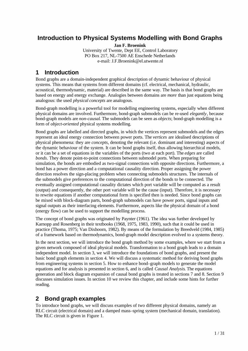
2 Bond graph examplesTo introduce bond graphs, we will discuss examples of two different physical domains, namely anRLC circuit (electrical domain) and a damped mass–spring system (mechanical domain, translation).The RLC circuit is given in Figure 1.

Intro Bond Graphs Jan F. Broenink, © 1999

2 / 31

Figure 1: The RLC circuit

In electrical networks, the port variables of the bond graph elements are the electrical voltage over theelement port and electrical current through the element port. Note that a port is an interface of anelement to other elements; it is the connection point of the bonds. The power being exchanged by aport with the rest of the system is the product of voltage and current: P = ui. The equations of aresistor, capacitor and inductor are:

∫∫

==

=

=

tuL

idtdi

Lu

tiC

u

iRu

LL

C

R

d1

or

d1

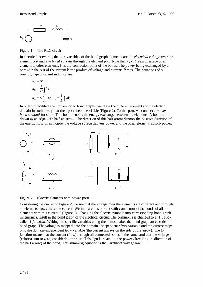
In order to facilitate the conversion to bond graphs, we draw the different elements of the electricdomain in such a way that their ports become visible (Figure 2). To this port, we connect a powerbond or bond for short. This bond denotes the energy exchange between the elements. A bond isdrawn as an edge with half an arrow. The direction of this half arrow denotes the positive direction ofthe energy flow. In principle, the voltage source delivers power and the other elements absorb power.

R

L C

C

+ +

++

_ _

__

i

i

i

i

i

i

ii

L

u

u

u

u

u

u

uu

R

Figure 2: Electric elements with power ports

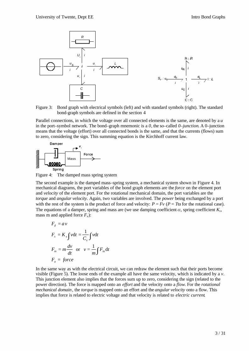
Considering the circuit of Figure 2, we see that the voltage over the elements are different and throughall elements flows the same current. We indicate this current with i and connect the bonds of allelements with this current I (Figure 3). Changing the electric symbols into corresponding bond graphmnemonics, result in the bond graph of the electrical circuit. The common i is changed to a ‘1’, a so-called 1-junction. Writing the specific variables along the bonds makes the bond graph an electricbond graph. The voltage is mapped onto the domain–independent effort variable and the current mapsonto the domain–independent flow variable (the current always on the side of the arrow). The 1-junction means that the current (flow) through all connected bonds is the same, and that the voltages(efforts) sum to zero, considering the sign. This sign is related to the power direction (i.e. direction ofthe half arrow) of the bond. This summing equation is the Kirchhoff voltage law.

Us

R

C

L

University of Twente, Dept EE Intro Bond Graphs

3 / 31

Figure 3: Bond graph with electrical symbols (left) and with standard symbols (right). The standardbond-graph symbols are defined in the section 4

Parallel connections, in which the voltage over all connected elements is the same, are denoted by a uin the port–symbol network. The bond–graph mnemonic is a 0, the so–called 0–junction. A 0–junctionmeans that the voltage (effort) over all connected bonds is the same, and that the currents (flows) sumto zero, considering the sign. This summing equation is the Kirchhoff current law.

Figure 4: The damped mass spring system

The second example is the damped mass–spring system, a mechanical system shown in Figure 4. Inmechanical diagrams, the port variables of the bond graph elements are the force on the element portand velocity of the element port. For the rotational mechanical domain, the port variables are thetorque and angular velocity. Again, two variables are involved. The power being exchanged by a portwith the rest of the system is the product of force and velocity: P = Fv (P = Tω for the rotational case).The equations of a damper, spring and mass are (we use damping coefficient α, spring coefficient Ks,mass m and applied force Fa):

forceF

tFm

vdtdv

mF

tvC

tvKF

vF

a

m

sss

d

=

==

==

=

∫

∫∫

d1

or

d1

d

m

α

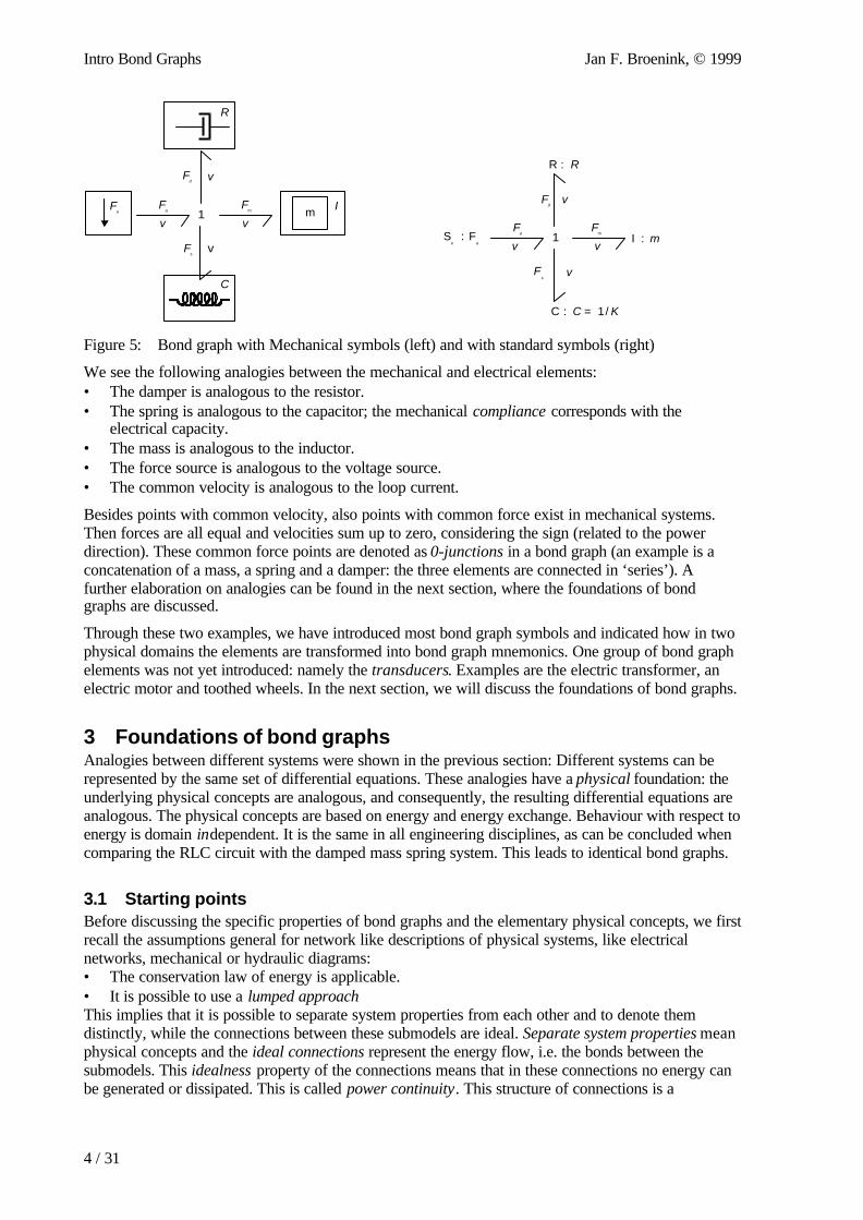
In the same way as with the electrical circuit, we can redraw the element such that their ports becomevisible (Figure 5). The loose ends of the example all have the same velocity, which is indicated by a v.This junction element also implies that the forces sum up to zero, considering the sign (related to thepower direction). The force is mapped onto an effort and the velocity onto a flow. For the rotationalmechanical domain , the torque is mapped onto an effort and the angular velocity onto a flow. Thisimplies that force is related to electric voltage and that velocity is related to electric current.

Spring

Mass

Damper

Force

v1

Spring

Mass

Damper

Force

v1

R

L

C

ii i

i

i

us uL

UR

uC


4 / 31

1v v

v

v

FaF

aF

m

Fd

Fs

m

R

C

I

R : R

I : m

C : = 1/C K

1v v

v

v

FaS : F

e a

Fm

Fd

Fs

Figure 5: Bond graph with Mechanical symbols (left) and with standard symbols (right)

We see the following analogies between the mechanical and electrical elements:• The damper is analogous to the resistor.• The spring is analogous to the capacitor; the mechanical compliance corresponds with the

electrical capacity.• The mass is analogous to the inductor.• The force source is analogous to the voltage source.• The common velocity is analogous to the loop current.

Besides points with common velocity, also points with common force exist in mechanical systems.Then forces are all equal and velocities sum up to zero, considering the sign (related to the powerdirection). These common force points are denoted as 0-junctions in a bond graph (an example is aconcatenation of a mass, a spring and a damper: the three elements are connected in ‘series’). Afurther elaboration on analogies can be found in the next section, where the foundations of bondgraphs are discussed.

Through these two examples, we have introduced most bond graph symbols and indicated how in twophysical domains the elements are transformed into bond graph mnemonics. One group of bond graphelements was not yet introduced: namely the transducers. Examples are the electric transformer, anelectric motor and toothed wheels. In the next section, we will discuss the foundations of bond graphs.

3 Foundations of bond graphsAnalogies between different systems were shown in the previous section: Different systems can berepresented by the same set of differential equations. These analogies have a physical foundation: theunderlying physical concepts are analogous, and consequently, the resulting differential equations areanalogous. The physical concepts are based on energy and energy exchange. Behaviour with respect toenergy is domain independent. It is the same in all engineering disciplines, as can be concluded whencomparing the RLC circuit with the damped mass spring system. This leads to identical bond graphs.

3.1 Starting pointsBefore discussing the specific properties of bond graphs and the elementary physical concepts, we firstrecall the assumptions general for network like descriptions of physical systems, like electricalnetworks, mechanical or hydraulic diagrams:• The conservation law of energy is applicable.• It is possible to use a lumped approachThis implies that it is possible to separate system properties from each other and to denote themdistinctly, while the connections between these submodels are ideal. Separate system properties meanphysical concepts and the ideal connections represent the energy flow, i.e. the bonds between thesubmodels. This idealness property of the connections means that in these connections no energy canbe generated or dissipated. This is called power continuity. This structure of connections is a


5 / 31

conceptual structure, which does not necessary have a size. This concept is called reticulation(Paynter, 1961) or tearing (Kron, 1963).

The system’s submodels are concepts, idealised descriptions of physical phenomena, which arerecognised as the dominating behaviour in components (i.e. real–life, tangible system parts). Thisimplies that a model of a concrete part is not necessary only one concept, but can consist of a set ofinterconnected concepts.

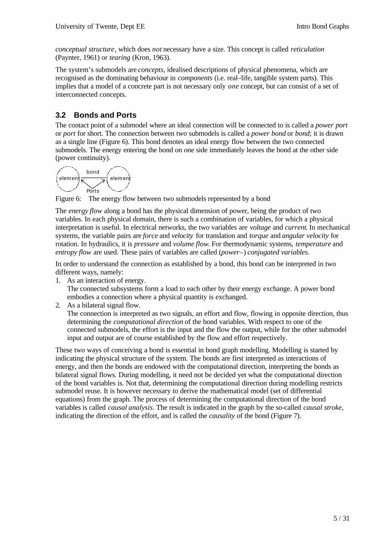
3.2 Bonds and PortsThe contact point of a submodel where an ideal connection will be connected to is called a power portor port for short. The connection between two submodels is called a power bond or bond; it is drawnas a single line (Figure 6). This bond denotes an ideal energy flow between the two connectedsubmodels. The energy entering the bond on one side immediately leaves the bond at the other side(power continuity).

Figure 6: The energy flow between two submodels represented by a bond

The energy flow along a bond has the physical dimension of power, being the product of twovariables. In each physical domain, there is such a combination of variables, for which a physicalinterpretation is useful. In electrical networks, the two variables are voltage and current. In mechanicalsystems, the variable pairs are force and velocity for translation and torque and angular velocity forrotation. In hydraulics, it is pressure and volume flow. For thermodynamic systems, temperature andentropy flow are used. These pairs of variables are called (power–) conjugated variables.

In order to understand the connection as established by a bond, this bond can be interpreted in twodifferent ways, namely:1. As an interaction of energy.

The connected subsystems form a load to each other by their energy exchange. A power bondembodies a connection where a physical quantity is exchanged.

2. As a bilateral signal flow.The connection is interpreted as two signals, an effort and flow, flowing in opposite direction, thusdetermining the computational direction of the bond variables. With respect to one of theconnected submodels, the effort is the input and the flow the output, while for the other submodelinput and output are of course established by the flow and effort respectively.

These two ways of conceiving a bond is essential in bond graph modelling. Modelling is started byindicating the physical structure of the system. The bonds are first interpreted as interactions ofenergy, and then the bonds are endowed with the computational direction, interpreting the bonds asbilateral signal flows. During modelling, it need not be decided yet what the computational directionof the bond variables is. Not that, determining the computational direction during modelling restrictssubmodel reuse. It is however necessary to derive the mathematical model (set of differentialequations) from the graph. The process of determining the computational direction of the bondvariables is called causal analysis. The result is indicated in the graph by the so-called causal stroke,indicating the direction of the effort, and is called the causality of the bond (Figure 7).

Ports

elementelementbond


6 / 31

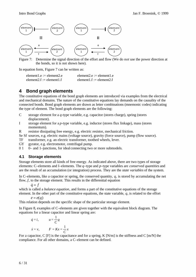
Figure 7: Determine the signal direction of the effort and flow (We do not use the power direction atthe bonds, so it is not shown here).

In equation form, Figure 7 can be written as:

element1.e := element2.e element2.e := element1.eelement2.f := element1.f element1.f := element2.f

4 Bond graph elementsThe constitutive equations of the bond graph elements are introduced via examples from the electricaland mechanical domains. The nature of the constitutive equations lay demands on the causality of theconnected bonds. Bond graph elements are drawn as letter combinations (mnemonic codes) indicatingthe type of element. The bond graph elements are the following:

C storage element for a q-type variable, e.g. capacitor (stores charge), spring (storesdisplacement).

I storage element for a p-type variable, e.g. inductor (stores flux linkage), mass (storesmomentum).

R resistor dissipating free energy, e.g. electric resistor, mechanical friction.Se Sf sources, e.g. electric mains (voltage source), gravity (force source), pump (flow source).TF transformer, e.g. an electric transformer, toothed wheels, lever.GY gyrator, e.g. electromotor, centrifugal pump.0 1 0– and 1–junctions, for ideal connecting two or more submodels.

4.1 Storage elementsStorage elements store all kinds of free energy. As indicated above, there are two types of storageelements: C–elements and I–elements. The q–type and p–type variables are conserved quantities andare the result of an accumulation (or integration) process. They are the state variables of the system.

In C–elements, like a capacitor or spring, the conserved quantity, q, is stored by accumulating the netflow, f, to the storage element. This results in the differential equation

&q f=which is called a balance equation, and forms a part of the constitutive equations of the storageelement. In the other part of the constitutive equations, the state variable, q, is related to the effort

e e q= ( )This relation depends on the specific shape of the particular storage element.

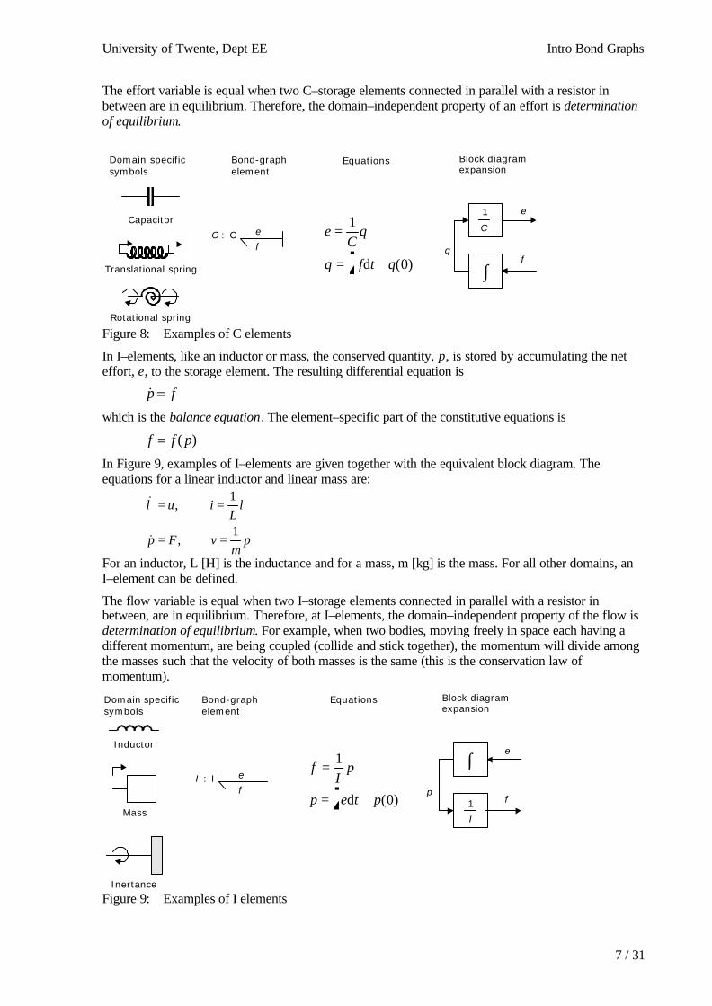
In Figure 8, examples of C–elements are given together with the equivalent block diagram. Theequations for a linear capacitor and linear spring are:

& ,

& ,

q i uC

q

x v F KxC

x

= =

= = =

1

1

For a capacitor, C [F] is the capacitance and for a spring, K [N/m] is the stiffness and C [m/N] thecompliance. For all other domains, a C–element can be defined.

e e

f f

element1

element1

element1

element1

element2

element2

element2

element2


7 / 31

The effort variable is equal when two C–storage elements connected in parallel with a resistor inbetween are in equilibrium. Therefore, the domain–independent property of an effort is determinationof equilibrium.

Figure 8: Examples of C elements

In I–elements, like an inductor or mass, the conserved quantity, p, is stored by accumulating the neteffort, e, to the storage element. The resulting differential equation is

&p f=which is the balance equation. The element–specific part of the constitutive equations is

f f p= ( )

In Figure 9, examples of I–elements are given together with the equivalent block diagram. Theequations for a linear inductor and linear mass are:

& ,

& ,

λ λ= =

= =

u iL

p F vm

p

1

1

For an inductor, L [H] is the inductance and for a mass, m [kg] is the mass. For all other domains, anI–element can be defined.

The flow variable is equal when two I–storage elements connected in parallel with a resistor inbetween, are in equilibrium. Therefore, at I–elements, the domain–independent property of the flow isdetermination of equilibrium. For example, when two bodies, moving freely in space each having adifferent momentum, are being coupled (collide and stick together), the momentum will divide amongthe masses such that the velocity of both masses is the same (this is the conservation law ofmomentum).

Figure 9: Examples of I elements

e

fC : C

e

f

1

C

q

∫

Domain specificsymbols

Bond-graph element

Block diagram expansion

Translational spring

Rotational spring

Capacitor

Equations

eC

q

q f t q

=

= +z1

0d ( )

fI

p

p e t p

=

= +z1

0d ( )

e

fI : I

e

f1

I

p

∫

Mass

Inertance

Inductor

Domain specificsymbols

Bond-graph element

Block diagram expansion

Equations


8 / 31

Note that when at the two types of storage elements, the role of effort and flow are exchanged: the C–element and the I–element are each other’s dual form.

The block diagrams in Figure 8 and 9, and also in the next Figures 10 to 16, show the computationaldirection of the signals involved. They are indeed the expansion of the corresponding causal bondgraph. The equations are given in computational form, consistent with the causal bond graph and theblock diagram.

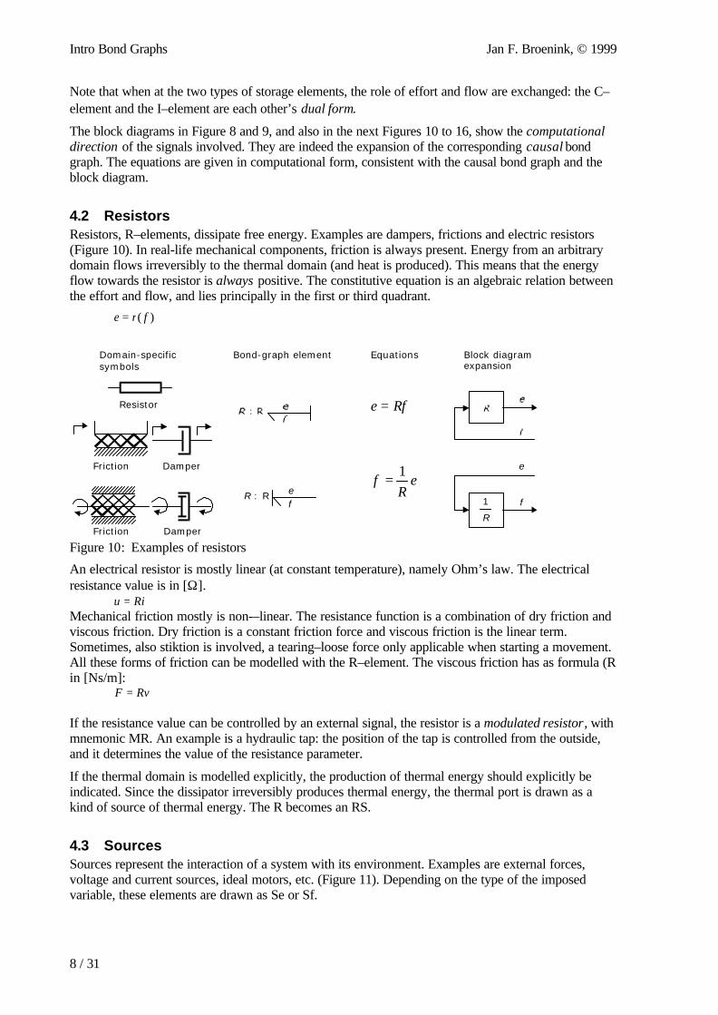
4.2 ResistorsResistors, R–elements, dissipate free energy. Examples are dampers, frictions and electric resistors(Figure 10). In real-life mechanical components, friction is always present. Energy from an arbitrarydomain flows irreversibly to the thermal domain (and heat is produced). This means that the energyflow towards the resistor is always positive. The constitutive equation is an algebraic relation betweenthe effort and flow, and lies principally in the first or third quadrant.

)( fre =

Figure 10: Examples of resistors

An electrical resistor is mostly linear (at constant temperature), namely Ohm’s law. The electricalresistance value is in [Ω].

Riu =Mechanical friction mostly is non-–linear. The resistance function is a combination of dry friction andviscous friction. Dry friction is a constant friction force and viscous friction is the linear term.Sometimes, also stiktion is involved, a tearing–loose force only applicable when starting a movement.All these forms of friction can be modelled with the R–element. The viscous friction has as formula (Rin [Ns/m]:

RvF =

If the resistance value can be controlled by an external signal, the resistor is a modulated resistor, withmnemonic MR. An example is a hydraulic tap: the position of the tap is controlled from the outside,and it determines the value of the resistance parameter.

If the thermal domain is modelled explicitly, the production of thermal energy should explicitly beindicated. Since the dissipator irreversibly produces thermal energy, the thermal port is drawn as akind of source of thermal energy. The R becomes an RS.

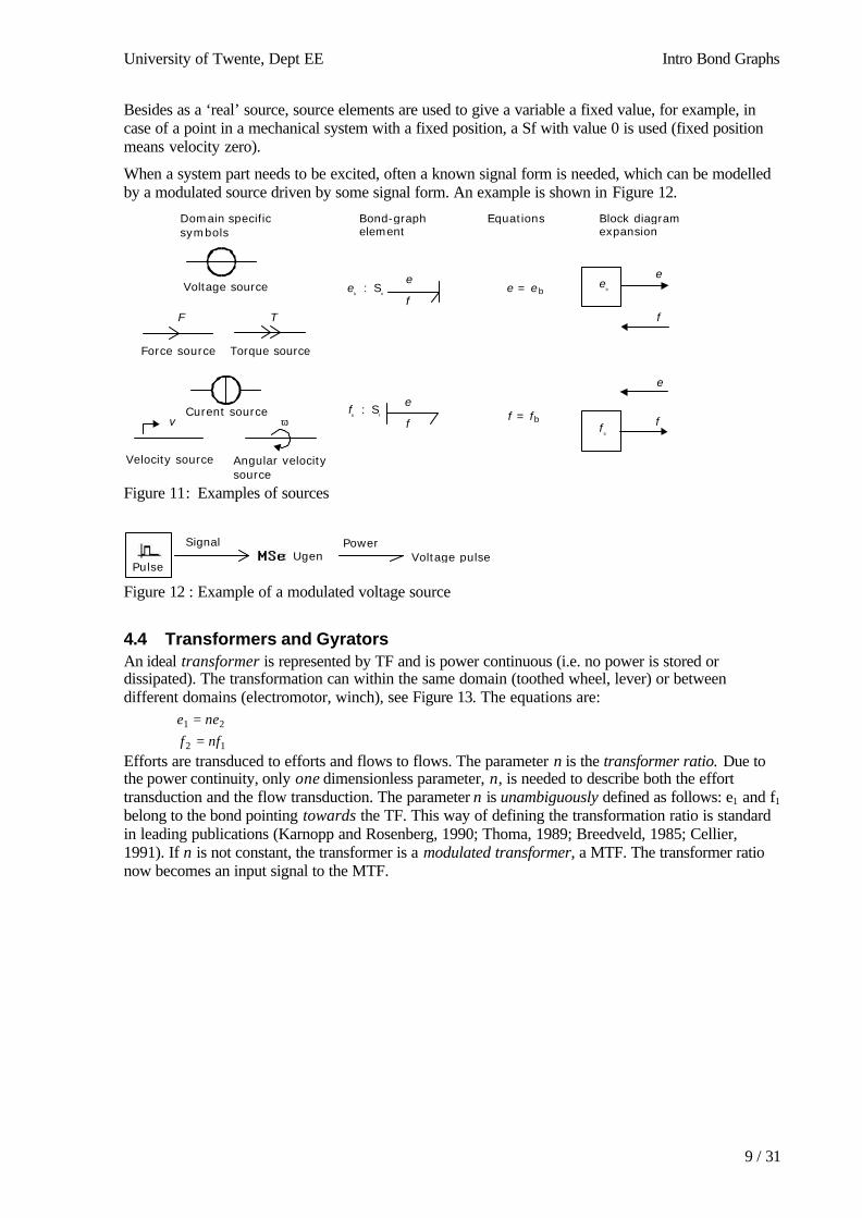
4.3 SourcesSources represent the interaction of a system with its environment. Examples are external forces,voltage and current sources, ideal motors, etc. (Figure 11). Depending on the type of the imposedvariable, these elements are drawn as Se or Sf.

1

R

e

fef

R : R

Damper

Resistor

Damper

Friction

Friction

Domain-specificsymbols

Bond-graph element Block diagram expansion

Equations

e Rf

fR

e

=

=1


9 / 31

Besides as a ‘real’ source, source elements are used to give a variable a fixed value, for example, incase of a point in a mechanical system with a fixed position, a Sf with value 0 is used (fixed positionmeans velocity zero).

When a system part needs to be excited, often a known signal form is needed, which can be modelledby a modulated source driven by some signal form. An example is shown in Figure 12.

Figure 11: Examples of sources

Figure 12 : Example of a modulated voltage source

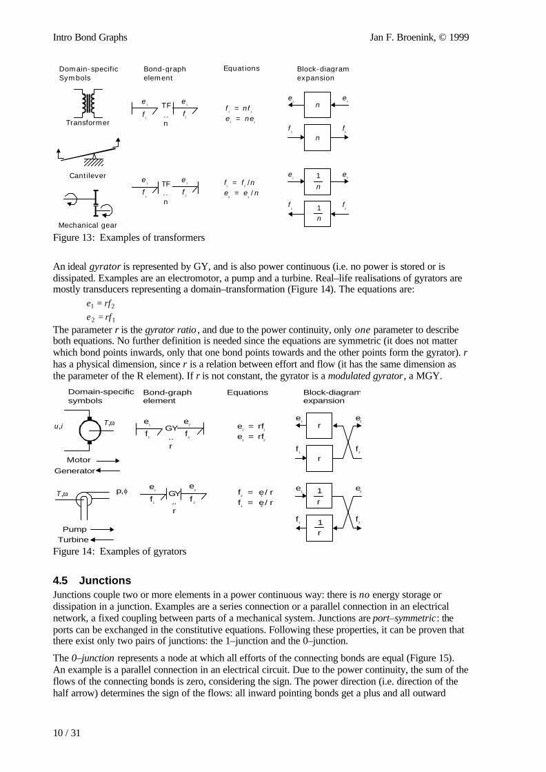
4.4 Transformers and GyratorsAn ideal transformer is represented by TF and is power continuous (i.e. no power is stored ordissipated). The transformation can within the same domain (toothed wheel, lever) or betweendifferent domains (electromotor, winch), see Figure 13. The equations are:

12

21

nffnee

==

Efforts are transduced to efforts and flows to flows. The parameter n is the transformer ratio. Due tothe power continuity, only one dimensionless parameter, n, is needed to describe both the efforttransduction and the flow transduction. The parameter n is unambiguously defined as follows: e1 and f1

belong to the bond pointing towards the TF. This way of defining the transformation ratio is standardin leading publications (Karnopp and Rosenberg, 1990; Thoma, 1989; Breedveld, 1985; Cellier,1991). If n is not constant, the transformer is a modulated transformer, a MTF. The transformer rationow becomes an input signal to the MTF.

Voltage pulsePowerSignal

: UgenPulse

eb e : S

e

f

ee

b

f

fb f : S

e

f

e

ffb

e e= b

f f= b

Voltage source

Curent source

Torque source

T

Force source

F

Angular velocitysource

ω

Velocity source

v

Domain specific symbols

Bond-graphelement

Block diagramexpansion

Equations


10 / 31

Figure 13: Examples of transformers

An ideal gyrator is represented by GY, and is also power continuous (i.e. no power is stored or isdissipated. Examples are an electromotor, a pump and a turbine. Real–life realisations of gyrators aremostly transducers representing a domain–transformation (Figure 14). The equations are:

12

21

rferfe

==

The parameter r is the gyrator ratio , and due to the power continuity, only one parameter to describeboth equations. No further definition is needed since the equations are symmetric (it does not matterwhich bond points inwards, only that one bond points towards and the other points form the gyrator). rhas a physical dimension, since r is a relation between effort and flow (it has the same dimension asthe parameter of the R element). If r is not constant, the gyrator is a modulated gyrator, a MGY.

Figure 14: Examples of gyrators

4.5 JunctionsJunctions couple two or more elements in a power continuous way: there is no energy storage ordissipation in a junction. Examples are a series connection or a parallel connection in an electricalnetwork, a fixed coupling between parts of a mechanical system. Junctions are port–symmetric: theports can be exchanged in the constitutive equations. Following these properties, it can be proven thatthere exist only two pairs of junctions: the 1–junction and the 0–junction.

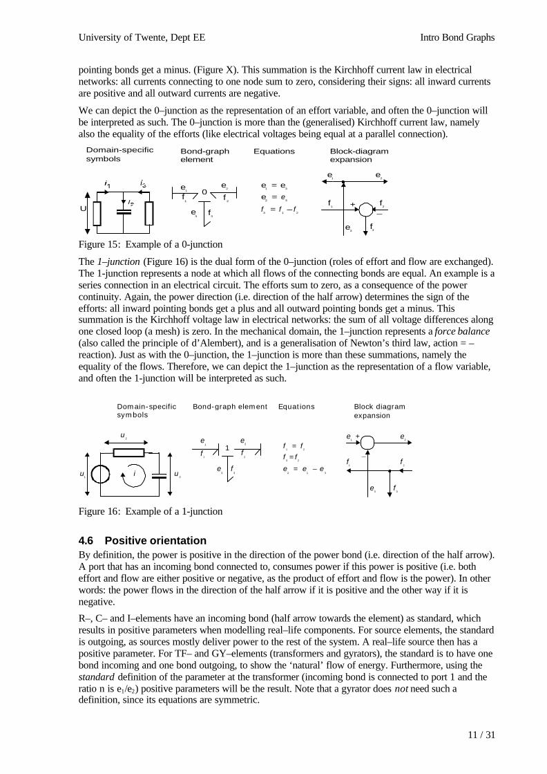
The 0–junction represents a node at which all efforts of the connecting bonds are equal (Figure 15).An example is a parallel connection in an electrical circuit. Due to the power continuity, the sum of theflows of the connecting bonds is zero, considering the sign. The power direction (i.e. direction of thehalf arrow) determines the sign of the flows: all inward pointing bonds get a plus and all outward

T,ω

T,ωu i,

MotorGenerator

PumpTurbine

e1

e2

f1

f2

GY..r

e1

e2

f1

f2

GY..r

e2

e1

f2

f1

r

r

1r

1r

e2

e1

f2

f1

e rfe rf

2 1

1 2

==

f e rf e r

2 1

1 2

= /= /


Bond-graph element

Block-diagramexpansion

p,ϕ

Equations

1n

1n

e2

e1

f2

f1

e2

e1

f2

f1

n

n

e1

e2

f1

f2

TF..n

f nfe ne

2 1

1 2

==

e1

e2

f1

f2

TF..n

f f ne e n

1 2

2 1

= /= /

Mechanical gear

Transformer

Cantilever

Domain-specificSymbols

Bond-graph element

Block-diagramexpansion

Equations


11 / 31

pointing bonds get a minus. (Figure X). This summation is the Kirchhoff current law in electricalnetworks: all currents connecting to one node sum to zero, considering their signs: all inward currentsare positive and all outward currents are negative.

We can depict the 0–junction as the representation of an effort variable, and often the 0–junction willbe interpreted as such. The 0–junction is more than the (generalised) Kirchhoff current law, namelyalso the equality of the efforts (like electrical voltages being equal at a parallel connection).

Figure 15: Example of a 0-junction

The 1–junction (Figure 16) is the dual form of the 0–junction (roles of effort and flow are exchanged).The 1-junction represents a node at which all flows of the connecting bonds are equal. An example is aseries connection in an electrical circuit. The efforts sum to zero, as a consequence of the powercontinuity. Again, the power direction (i.e. direction of the half arrow) determines the sign of theefforts: all inward pointing bonds get a plus and all outward pointing bonds get a minus. Thissummation is the Kirchhoff voltage law in electrical networks: the sum of all voltage differences alongone closed loop (a mesh) is zero. In the mechanical domain, the 1–junction represents a force balance(also called the principle of d’Alembert), and is a generalisation of Newton’s third law, action = –reaction). Just as with the 0–junction, the 1–junction is more than these summations, namely theequality of the flows. Therefore, we can depict the 1–junction as the representation of a flow variable,and often the 1-junction will be interpreted as such.

e1

e2

e3

f1

f2

f3

1

e e e2 1 3

= –

f f 3 2=

f f1 2

=e

1e

2

e3

f1

f2

f3

+

_


Bond-graph element Block diagram expansion

u1

u3

u2

i

Equations

Figure 16: Example of a 1-junction

4.6 Positive orientationBy definition, the power is positive in the direction of the power bond (i.e. direction of the half arrow).A port that has an incoming bond connected to, consumes power if this power is positive (i.e. botheffort and flow are either positive or negative, as the product of effort and flow is the power). In otherwords: the power flows in the direction of the half arrow if it is positive and the other way if it isnegative.

R–, C– and I–elements have an incoming bond (half arrow towards the element) as standard, whichresults in positive parameters when modelling real–life components. For source elements, the standardis outgoing, as sources mostly deliver power to the rest of the system. A real–life source then has apositive parameter. For TF– and GY–elements (transformers and gyrators), the standard is to have onebond incoming and one bond outgoing, to show the ‘natural’ flow of energy. Furthermore, using thestandard definition of the parameter at the transformer (incoming bond is connected to port 1 and theratio n is e1/e2) positive parameters will be the result. Note that a gyrator does not need such adefinition, since its equations are symmetric.

e1

e2

e3

f1

f2

f3

0e e

1 3=

f f f3 1 2 = –

e = 2 3

e

e1

e2

e3

f1

f2

f3

+_


Bond-graph element

Block-diagram expansion

U

Equations


12 / 31

It is possible, however, that negative parameters occur. Namely, at transformers and sources in themechanical domain when there is a reverse of velocity or the source acts in the negative direction.

Using the definitions discussed in this section, the bond–graph definition is unambiguous, implyingthat in principle there is no need for confusion. Furthermore, this systematic way will help resolvingpossible sign–placing problems often encountered in modelling.

4.7 Duality and dual domainsAs indicated in section 4.1, the two storage elements are each other’s dual form. The role of effort andflow in a C–element and I–element are exchanged. Leaving one of the storage elements (and also oneof the sources) out of the list of bond graph elements, to make this list as small as possible, can beuseful from a mathematical viewpoint, but does not enhance the insight in physics.

Decomposing an I–element into a GY and a C, though, gives more insight. The only storage elementnow is the C–element. The flow is only a time derivative of a conserved quantity, and the effortdetermines the equilibrium. This implies that the physical domains are actually pairs of two dualdomains: in mechanics, we have potential and kinetic domains for both rotation and translation), inelectrical networks, we have the electrical and magnetic domains. However, in the thermodynamicdomain, no such dual form exists (Breedveld, 1982). This is consistent with the fact that no thermal I–type storage exists (as a consequence of the second law of thermodynamics: in a thermally isolatedsystem, the entropy never decreases).

4.8 OverviewWe have discussed the basic bond–graph elements and the bonds, so we can transform a domain–dependent ideal–physical model, written in domain–dependent symbols, into a bond graph. For thistransformation, there is a systematic procedure, which will be presented in the next section.

5 Systematic procedure to derive a bond–graph model

To generate a bond–graph model starting from an ideal–physical model, a systematic method exist,which we will present here as a procedure. This procedure consists roughly of the identification of thedomains and basic elements, the generation of the connection structure (called the junction structure),the placement of the elements, and possibly simplifying the graph. The procedure is different for themechanical domain compared to the other domains. These differences are indicated betweenparenthesis. The reason is that elements need to be connected to difference variables or acrossvariables. The efforts in the non–mechanical domains and the velocities (flows) in the mechanicaldomains are the across variables we need.

Step 1 and 2 concern the identification of the domains and elements.

1 Determine which physical domains exist in the system and identify all basic elements like C, I,R, Se, Sf, TF and GY.Give every element a unique name to distinguish them from each other.

2 Indicate in the ideal–physical model per domain a reference effort (reference velocity withpositive direction for the mechanical domains).Note that only the references in the mechanical domains have a direction.

Steps 3 through 6 describe the generation of the connection structure (called the junction structure).

3 Identify all other efforts (mechanical domains: velocities) and give them unique names.4 Draw these efforts (mechanical: velocities), and not the references, graphically by 0–junctions

(mechanical: 1–junctions). Keep if possible, the same layout as the IPM.5 Identify all effort differences (mechanical: velocity (= flow) differences) needed to connect the

ports of all elements enumerated in step 1 to the junction structure.


13 / 31

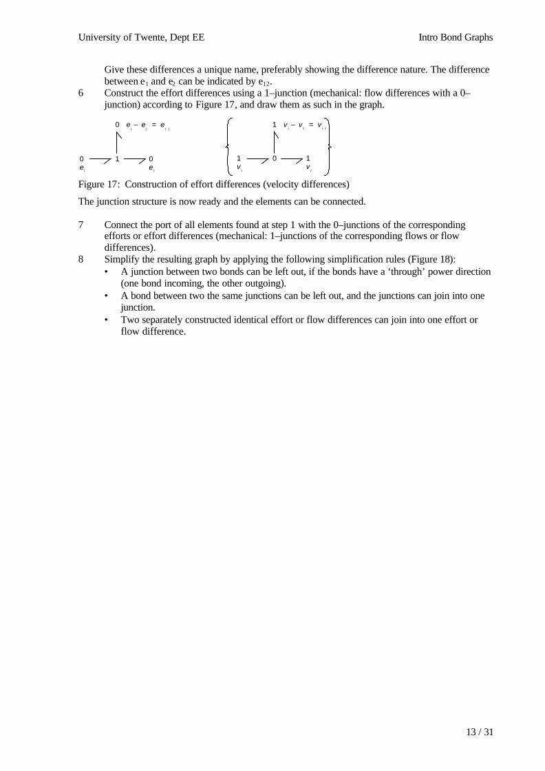
Give these differences a unique name, preferably showing the difference nature. The differencebetween e1 and e2 can be indicated by e12.

6 Construct the effort differences using a 1–junction (mechanical: flow differences with a 0–junction) according to Figure 17, and draw them as such in the graph.

Figure 17: Construction of effort differences (velocity differences)

The junction structure is now ready and the elements can be connected.

7 Connect the port of all elements found at step 1 with the 0–junctions of the correspondingefforts or effort differences (mechanical: 1–junctions of the corresponding flows or flowdifferences).

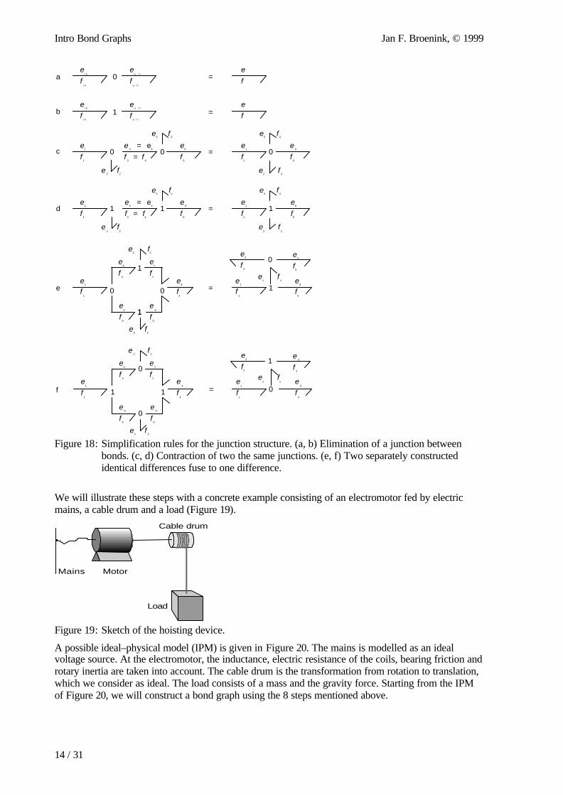
8 Simplify the resulting graph by applying the following simplification rules (Figure 18):• A junction between two bonds can be left out, if the bonds have a ‘through’ power direction

(one bond incoming, the other outgoing).• A bond between two the same junctions can be left out, and the junctions can join into one

junction.• Two separately constructed identical effort or flow differences can join into one effort or

flow difference.

0

0

e2

e1

e – e = e1 2 1 2

1 1

1

v2

v1

v – v = v1 2 1 2

0 10


14 / 31

Figure 18: Simplification rules for the junction structure. (a, b) Elimination of a junction betweenbonds. (c, d) Contraction of two the same junctions. (e, f) Two separately constructedidentical differences fuse to one difference.

We will illustrate these steps with a concrete example consisting of an electromotor fed by electricmains, a cable drum and a load (Figure 19).

Figure 19: Sketch of the hoisting device.

A possible ideal–physical model (IPM) is given in Figure 20. The mains is modelled as an idealvoltage source. At the electromotor, the inductance, electric resistance of the coils, bearing friction androtary inertia are taken into account. The cable drum is the transformation from rotation to translation,which we consider as ideal. The load consists of a mass and the gravity force. Starting from the IPMof Figure 20, we will construct a bond graph using the 8 steps mentioned above.

Load

Cable drum

MotorMains

0

1

=

=

a

b

c

d

e

f

ei n

ei n

fi n

fi n

0 00 =e

1e

1e

6e

6

e2

e2

e5

e5

e3 4 = e

f1

f1

f6

f6

f2

f2

f5

f5

f f3 4

=

1 11 =e

1e

1e

6e

6

e2

e2

e5

e5

e3 4 = e

f1

f1

f6

f6

f2

f2

0 0

0

1

1

1

1

=e

1

ea

eb

ec

ed

e4

e4

e1

e2 e

3

e3

e2

f1

fa

fb

fc

fd

f4

f4

f1

f2 f

3

f3

f2

1 1

1

0

0

0

=e

1

ea

eb

ec

ed

e4

e4

e1

e2 e

3

e3

e2

ex

ex

f1

fa

fb

fc

fd

f4

f4

f1

f2 f

3

f3

f2

fx

fx

f5

f5

f f3 4

=

eu i t

eu i t

fu i t

fu i t

e

e

f

f


15 / 31

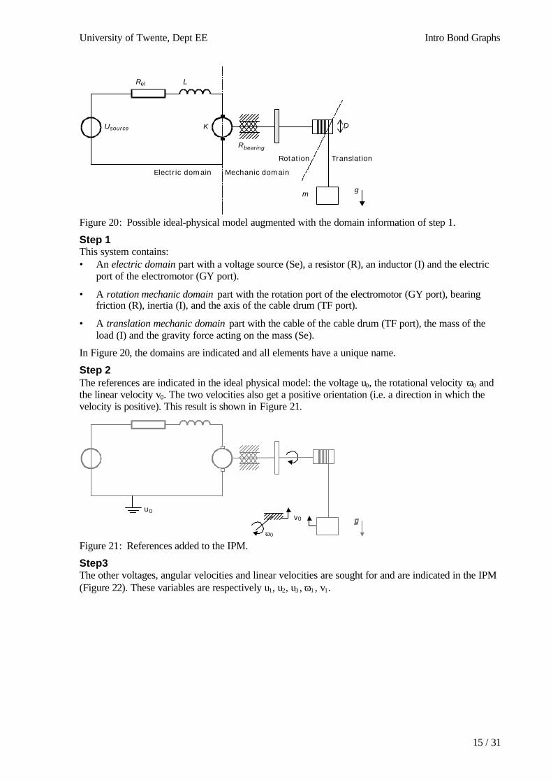
Figure 20: Possible ideal-physical model augmented with the domain information of step 1.

Step 1This system contains:• An electric domain part with a voltage source (Se), a resistor (R), an inductor (I) and the electric

port of the electromotor (GY port).

• A rotation mechanic domain part with the rotation port of the electromotor (GY port), bearingfriction (R), inertia (I), and the axis of the cable drum (TF port).

• A translation mechanic domain part with the cable of the cable drum (TF port), the mass of theload (I) and the gravity force acting on the mass (Se).

In Figure 20, the domains are indicated and all elements have a unique name.

Step 2The references are indicated in the ideal physical model: the voltage u0, the rotational velocity ω0 andthe linear velocity v0. The two velocities also get a positive orientation (i.e. a direction in which thevelocity is positive). This result is shown in Figure 21.

Figure 21: References added to the IPM.

Step3The other voltages, angular velocities and linear velocities are sought for and are indicated in the IPM(Figure 22). These variables are respectively u1, u2, u3 , ω1 , v1.

v0

ω0

u0

g

Rel L

Rbearing

D

m

Electric domain Mechanic domain

Rotation Translation

Usource K


16 / 31

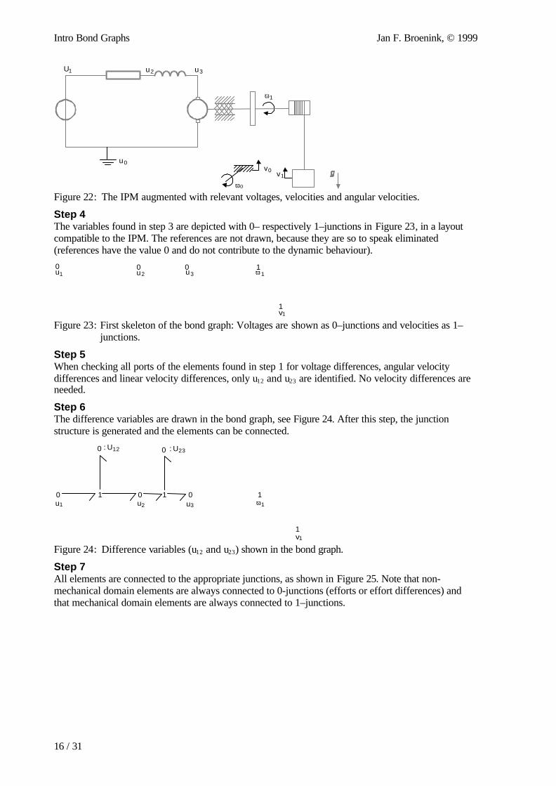
Figure 22: The IPM augmented with relevant voltages, velocities and angular velocities.

Step 4The variables found in step 3 are depicted with 0– respectively 1–junctions in Figure 23, in a layoutcompatible to the IPM. The references are not drawn, because they are so to speak eliminated(references have the value 0 and do not contribute to the dynamic behaviour).

Figure 23: First skeleton of the bond graph: Voltages are shown as 0–junctions and velocities as 1–junctions.

Step 5When checking all ports of the elements found in step 1 for voltage differences, angular velocitydifferences and linear velocity differences, only u12 and u23 are identified. No velocity differences areneeded.

Step 6The difference variables are drawn in the bond graph, see Figure 24. After this step, the junctionstructure is generated and the elements can be connected.

Figure 24: Difference variables (u12 and u23) shown in the bond graph.

Step 7All elements are connected to the appropriate junctions, as shown in Figure 25. Note that non-mechanical domain elements are always connected to 0-junctions (efforts or effort differences) andthat mechanical domain elements are always connected to 1–junctions.

v0

ω0

u0

U1 u2 u3

ω1

v1

ω11

u30

u2u100

v11

:U12 :U23

u1 u2 u3 ω1

v1

0 0 0 1

1

1 1

0 0


17 / 31

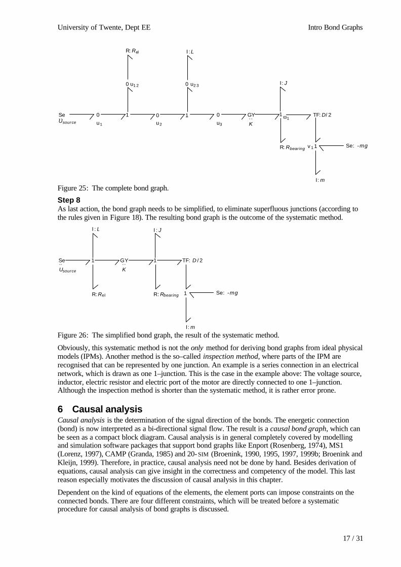
Figure 25: The complete bond graph.

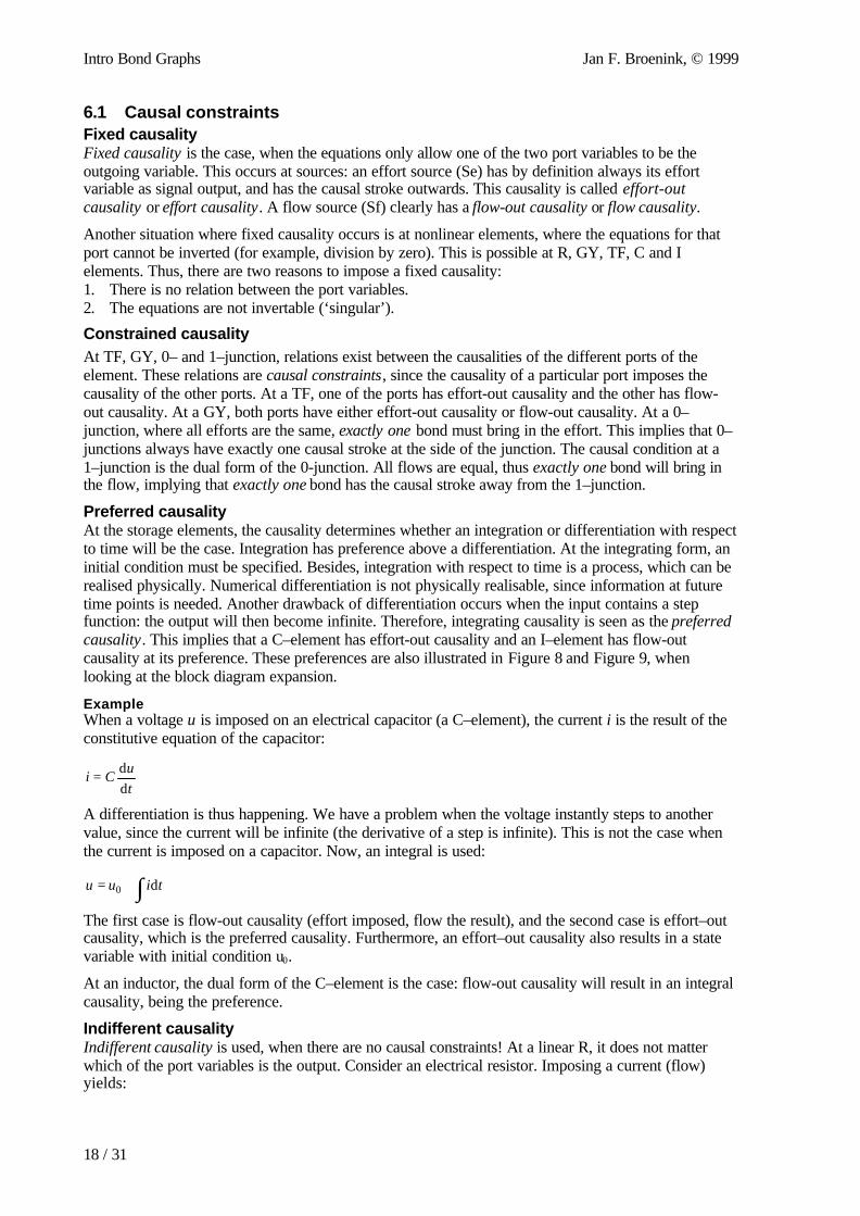
Step 8As last action, the bond graph needs to be simplified, to eliminate superfluous junctions (according tothe rules given in Figure 18). The resulting bond graph is the outcome of the systematic method.

Figure 26: The simplified bond graph, the result of the systematic method.

Obviously, this systematic method is not the only method for deriving bond graphs from ideal physicalmodels (IPMs). Another method is the so–called inspection method, where parts of the IPM arerecognised that can be represented by one junction. An example is a series connection in an electricalnetwork, which is drawn as one 1–junction. This is the case in the example above: The voltage source,inductor, electric resistor and electric port of the motor are directly connected to one 1–junction.Although the inspection method is shorter than the systematic method, it is rather error prone.

6 Causal analysisCausal analysis is the determination of the signal direction of the bonds. The energetic connection(bond) is now interpreted as a bi-directional signal flow. The result is a causal bond graph, which canbe seen as a compact block diagram. Causal analysis is in general completely covered by modellingand simulation software packages that support bond graphs like Enport (Rosenberg, 1974), MS1(Lorenz, 1997), CAMP (Granda, 1985) and 20- SIM (Broenink, 1990, 1995, 1997, 1999b; Broenink andKleijn, 1999). Therefore, in practice, causal analysis need not be done by hand. Besides derivation ofequations, causal analysis can give insight in the correctness and competency of the model. This lastreason especially motivates the discussion of causal analysis in this chapter.

Dependent on the kind of equations of the elements, the element ports can impose constraints on theconnected bonds. There are four different constraints, which will be treated before a systematicprocedure for causal analysis of bond graphs is discussed.

u1 u2 u3

ω1

v1

u12 u23

..Usource

1

TF: /2D

Se: -mg

I:m

0 0 0 11 1

00

Se

R:Rel I:L

I:J

R:Rbearing

GY..K

..Usource

GY 1

1

1 TF: /2DSe

I:L

Se: -mg

I:m

I:J

R:RbearingR:Rel

..K


18 / 31

6.1 Causal constraintsFixed causalityFixed causality is the case, when the equations only allow one of the two port variables to be theoutgoing variable. This occurs at sources: an effort source (Se) has by definition always its effortvariable as signal output, and has the causal stroke outwards. This causality is called effort-outcausality or effort causality. A flow source (Sf) clearly has a flow-out causality or flow causality.

Another situation where fixed causality occurs is at nonlinear elements, where the equations for thatport cannot be inverted (for example, division by zero). This is possible at R, GY, TF, C and Ielements. Thus, there are two reasons to impose a fixed causality:1. There is no relation between the port variables.2. The equations are not invertable (‘singular’).

Constrained causalityAt TF, GY, 0– and 1–junction, relations exist between the causalities of the different ports of theelement. These relations are causal constraints, since the causality of a particular port imposes thecausality of the other ports. At a TF, one of the ports has effort-out causality and the other has flow-out causality. At a GY, both ports have either effort-out causality or flow-out causality. At a 0–junction, where all efforts are the same, exactly one bond must bring in the effort. This implies that 0–junctions always have exactly one causal stroke at the side of the junction. The causal condition at a1–junction is the dual form of the 0-junction. All flows are equal, thus exactly one bond will bring inthe flow, implying that exactly one bond has the causal stroke away from the 1–junction.

Preferred causalityAt the storage elements, the causality determines whether an integration or differentiation with respectto time will be the case. Integration has preference above a differentiation. At the integrating form, aninitial condition must be specified. Besides, integration with respect to time is a process, which can berealised physically. Numerical differentiation is not physically realisable, since information at futuretime points is needed. Another drawback of differentiation occurs when the input contains a stepfunction: the output will then become infinite. Therefore, integrating causality is seen as the preferredcausality. This implies that a C–element has effort-out causality and an I–element has flow-outcausality at its preference. These preferences are also illustrated in Figure 8 and Figure 9, whenlooking at the block diagram expansion.

ExampleWhen a voltage u is imposed on an electrical capacitor (a C–element), the current i is the result of theconstitutive equation of the capacitor:

tuCi

dd=

A differentiation is thus happening. We have a problem when the voltage instantly steps to anothervalue, since the current will be infinite (the derivative of a step is infinite). This is not the case whenthe current is imposed on a capacitor. Now, an integral is used:

∫+= tiuu d0

The first case is flow-out causality (effort imposed, flow the result), and the second case is effort–outcausality, which is the preferred causality. Furthermore, an effort–out causality also results in a statevariable with initial condition u0.

At an inductor, the dual form of the C–element is the case: flow-out causality will result in an integralcausality, being the preference.

Indifferent causalityIndifferent causality is used, when there are no causal constraints! At a linear R, it does not matterwhich of the port variables is the output. Consider an electrical resistor. Imposing a current (flow)yields:


19 / 31

iRu =

It is also possible to impose a voltage (effort) on the linear resistor:

Ru

i =

There is no difference choosing the current as incoming variable and the voltage as outgoing variable,or the other way around.

OverviewThe Se and Sf have a fixed causality, the C and I have a preferred causality, the TF, GY, 0 and 1 haveconstrained causality, and the R has an indifferent causality (provided that the equations of these basicelements all are invertable). These causal forms have been shown in section 4. When the equations arenot invertable, a fixed causality must be used.

6.2 Causal analysis procedureThe procedure for assigning causality on a bond graph starts with those elements that have thestrongest causality constraint namely fixed causality (deviation of the causality condition cannot begranted by rewriting the equations, since rewriting is not possible). Via the bonds (i.e. connections) inthe graph, one causality assignment can cause other causalities to be assigned. This effect is calledcausality propagation: after one assignment, the causality propagates through the bond graph due tothe causal constraints.

The causality assignment algorithm is as follows:

1a. Chose a fixed causality of a source element, assign its causality, and propagate this assignmentthrough the graph using the causal constraints. Go on until all sources have their causalitiesassigned.

1b. Chose a not yet causal port with fixed causality (non-invertable equations), assign its causality,and propagate this assignment through the graph using the causal constraints. Go on until all portswith fixed causality have their causalities assigned.

2. Chose a not yet causal port with preferred causality (storage elements), assign its causality, andpropagate this assignment through the graph using the causal constraints. Go on until all ports withpreferred causality have their causalities assigned.

3. Chose a not yet causal port with indifferent causality, assign its causality, and propagate thisassignment through the graph using the causal constraints. Go on until all ports with indifferentcausality have their causalities assigned.

Often, the bond graph is completely causal after step 2, without any causal conflict (all causalconditions are satisfied). If this is not the case, then the moment in the procedure where a conflictoccurs or where the graph becomes completely causal, can give insight in the correctness andcompetence of the model. Before discussing these issues, first an example will be treated.

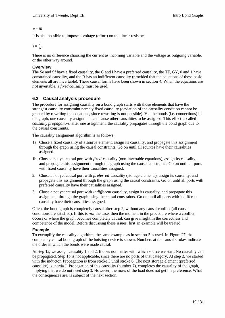
ExampleTo exemplify the causality algorithm, the same example as in section 5 is used. In Figure 27, thecompletely causal bond graph of the hoisting device is shown. Numbers at the causal strokes indicatethe order in which the bonds were made causal.

At step 1a, we assign causality 1 and 2. It does not matter with which source we start. No causality canbe propagated. Step 1b is not applicable, since there are no ports of that category. At step 2, we startedwith the inductor. Propagation is from stroke 3 until stroke 6. The next storage element (preferredcausality) is inertia J. Propagation of this causality (number 7), completes the causality of the graph,implying that we do not need step 3. However, the mass of the load does not get his preference. Whatthe consequences are, is subject of the next section.


20 / 31

Figure 27: The causal bond graph of the hoisting device

6.3 Model insight via causal analysisWe discuss here those situations whereby conflicts occur in the causal analysis procedure or when step3 of the algorithm appears to be necessary. The place in procedure where a conflict appears or thebond graph becomes completely causally augmented, can give insight in the correctness of the model.

Often, the bond graph is completely causal after step 2, without any causal conflict (all causalconditions are satisfied). Each storage element represents a state variable, and the set of equations is anexplicit set of ordinary differential equations (not necessarily linear or time invariant).

When the bond graph is completely causal after step 1a, the model does not have any dynamics. Thebehaviour of all variables now is determined by the fixed causalities of the sources. Arises a causalconflict at step 1a or at step 1b, then the problem is ill posed. The model must be changed, by addingsome elements. An example of a causal conflict at step 1a is two effort sources connected to one 0-junction. Both sources ‘want’ to determine the one effort variable.

At a conflict at step 1b, a possible adjustment is changing the equations of the fixed–causality elementsuch that these equations become invertable, and thus the fixedness of the constraint disappears. Anexample is a diode or a valve having zero current resp. flow while blocking. Allowing a smallresistance during blocking, the equations become invertable.

When a conflict arises at step 2, a storage element receives a non-–preferred causality. This means thatthis storage element does not represent a state variable. The initial value of this storage elementcannot be chosen freely. Such a storage element often is called a dependent storage element. Thisindicates that a storage element was not taken into account during modelling, which should be therefrom physical systems viewpoint. It can be deliberately omitted, or it might be forgotten. At thehoisting device example, the load of the hoist (I—element) is such a dependent storage element.Elasticity in the cable was not modelled. If it had been modelled, a C—storage element connected to a0—junction between the cable drum and load would appear.

When step 3 of the causality algorithm is necessary, a so—called algebraic loop is present in thegraph. This loop causes the resulting set differential equations to be implicit. Often this is an indicationthat a storage element was not modelled, which should be there from a physical systems viewpoint.

In general, different ways to handle the causal conflicts arising at step 2 or step 3 are possible:1. Add elements.

For example, you can withdraw the decision to neglect certain elements. The added elements canbe parasitic, for example, to add elasticity (C—element) in a mechanical connection, which wasmodelled as rigid. Additionally adding a damping element (R) reduces the simulation timeconsiderably, which is being advised.

2. Change the bond graph such that the conflict disappears.For a step 2 conflict, the dependent storage element is taken together with an independent storage

I:m

1R:RbearingR:Rel Se: -mg1

2

3

4

5 6

7

8

GY1Se

I:L

..K

..Usource

1

I:J

9

10

11

TF: /2D


21 / 31

element, having integral causality. For a step 3 conflict, sometimes resistive elements can be takentogether to eliminate the conflict. This can be performed via transformations in the graph. Thecomplexity of this operation depends on the size and kind of submodels along the route betweenthe storage elements or resistors under concern.

3. The bond graph is not changed and during simulation, a special (implicit) integration routine isneeded. The implicit equations are solved by means of the iteration schemes present in the implicitintegration methods. In 20-SIM, only the BDF method can handle this situation.Also, the loop can be ‘cut’ by adding a one-timestep delay, which is a rather pragmatic solution,but can be useful when no implicit integration methods are available. The accuracy might get toolow. Note that the amplification of all elements in the loop must be smaller than one to obtain astable solution.

Algebraic loops and loops between a dependent and an independent storage element are called zero–order causal paths (ZCPs). Besides these two kinds, there are three other kinds, having an increasingcomplexity and resulting in more complex equations. These occur for instance in rigid–bodymechanical systems (van Dijk and Breedveld, 1991).

By interpreting the result of causal analysis, several properties of the model can be recognised, whichcould otherwise only be done after deriving equations.

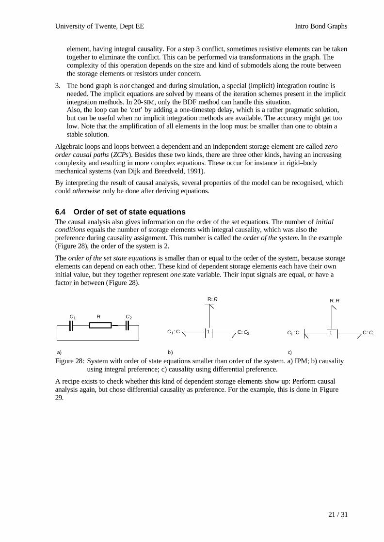
6.4 Order of set of state equationsThe causal analysis also gives information on the order of the set equations. The number of initialconditions equals the number of storage elements with integral causality, which was also thepreference during causality assignment. This number is called the order of the system. In the example(Figure 28), the order of the system is 2.

The order of the set state equations is smaller than or equal to the order of the system, because storageelements can depend on each other. These kind of dependent storage elements each have their owninitial value, but they together represent one state variable. Their input signals are equal, or have afactor in between (Figure 28).

Figure 28: System with order of state equations smaller than order of the system. a) IPM; b) causalityusing integral preference; c) causality using differential preference.

A recipe exists to check whether this kind of dependent storage elements show up: Perform causalanalysis again, but chose differential causality as preference. For the example, this is done in Figure29.

C1 C2R

C1:C C:C2

R:R

1 C1:C C:C2

R:R

1

a) b) c)


22 / 31

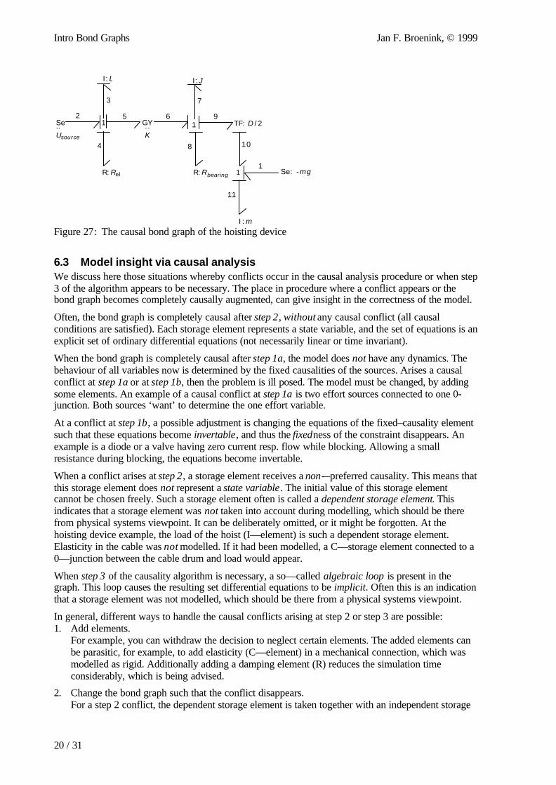
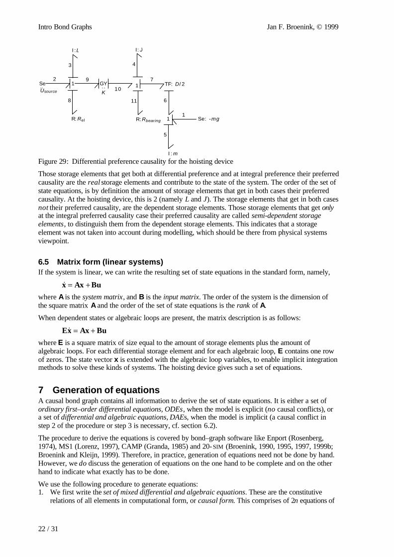
Figure 29: Differential preference causality for the hoisting device

Those storage elements that get both at differential preference and at integral preference their preferredcausality are the real storage elements and contribute to the state of the system. The order of the set ofstate equations, is by definition the amount of storage elements that get in both cases their preferredcausality. At the hoisting device, this is 2 (namely L and J). The storage elements that get in both casesnot their preferred causality, are the dependent storage elements. Those storage elements that get onlyat the integral preferred causality case their preferred causality are called semi-dependent storageelements, to distinguish them from the dependent storage elements. This indicates that a storageelement was not taken into account during modelling, which should be there from physical systemsviewpoint.

6.5 Matrix form (linear systems)If the system is linear, we can write the resulting set of state equations in the standard form, namely,

&x Ax Bu= +where A is the system matrix, and B is the input matrix. The order of the system is the dimension ofthe square matrix A and the order of the set of state equations is the rank of A.

When dependent states or algebraic loops are present, the matrix description is as follows:

Ex Ax Bu& = +where E is a square matrix of size equal to the amount of storage elements plus the amount ofalgebraic loops. For each differential storage element and for each algebraic loop, E contains one rowof zeros. The state vector x is extended with the algebraic loop variables, to enable implicit integrationmethods to solve these kinds of systems. The hoisting device gives such a set of equations.

7 Generation of equationsA causal bond graph contains all information to derive the set of state equations. It is either a set ofordinary first–order differential equations, ODEs, when the model is explicit (no causal conflicts), ora set of differential and algebraic equations, DAEs, when the model is implicit (a causal conflict instep 2 of the procedure or step 3 is necessary, cf. section 6.2).

The procedure to derive the equations is covered by bond–graph software like Enport (Rosenberg,1974), MS1 (Lorenz, 1997), CAMP (Granda, 1985) and 20- SIM (Broenink, 1990, 1995, 1997, 1999b;Broenink and Kleijn, 1999). Therefore, in practice, generation of equations need not be done by hand.However, we do discuss the generation of equations on the one hand to be complete and on the otherhand to indicate what exactly has to be done.

We use the following procedure to generate equations:1. We first write the set of mixed differential and algebraic equations. These are the constitutive

relations of all elements in computational form, or causal form. This comprises of 2n equations of

I:m

1R:RbearingR:Rel Se: -mg1

2

3

8

9

10

4

11

GY1Se

I:L

..K

..Usource

1

I:J

7

6

5

TF: /2D


23 / 31

a bond graph having n bonds. n equations compute an effort and n equations compute a flow, orderivatives of them.

2. We then eliminate the algebraic equations. We can organise this elimination process by firsteliminate the identities coming from the sources and junctions. Thereafter, we substitute themultiplications with a parameter, stemming from resistors and transducers (TF, GY). At last, wesubstitute the summation equations of the junctions into the differential equations of the storageelements. Within this process, it is efficient to first mark the state variables. In principle, the statevariables are the contents of the storage elements (p or q type variables). However, if we write theconstitutive relations of storage elements as one differential equation, we can also use the efforts atC-elements and flows at I-elements.

If we are going to generate the equations by hand, we can take the first elimination step into accountwhile formulating the equations by, at the sources, directly use the signal function at the bond.Furthermore, we can write the variable determining the junction along all bonds connected to thatjunction. The variable determining the junction is that variable, which gets assigned to bond variablesof all the other bonds connected to that junction via the identities of the junction equations. At a 0–junction, this is the effort of the only bond with its causal stroke towards the 0-junction. At a 1–junction, this is the flow of the only bond with its causal stroke away from the 1-junction.

In case of dependent storage elements, we have to take care that the accompanying state variable getsnot eliminated. These are the so–called semi state variables. When we mark the state variables,including the semi state variables in this situation, on beforehand, we can prevent the wrong variablefrom being eliminated. In case of algebraic loops, implicit equations will be encountered. We chooseone of the variables in these loops as algebraic loop breaker and that variable becomes a semi statevariable. See also section 6.5. The equation consisting the semi state variable of a storage element getseliminated at the second elimination step: it is a multiplication. The semi state variable itself must notbe substituted.

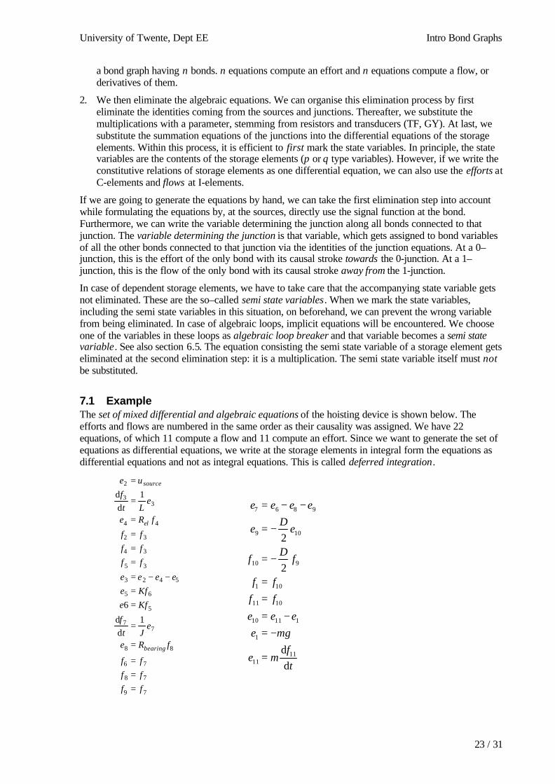
7.1 ExampleThe set of mixed differential and algebraic equations of the hoisting device is shown below. Theefforts and flows are numbered in the same order as their causality was assigned. We have 22equations, of which 11 compute a flow and 11 compute an effort. Since we want to generate the set ofequations as differential equations, we write at the storage elements in integral form the equations asdifferential equations and not as integral equations. This is called deferred integration.

79

78

76

88

77

5

65

5423

35

34

32

44

33

2

1dd

6

1dd

ffffff

fRe

eJt

f

KfeKfe

eeee

ffffff

fRe

eLt

fue

bearing

el

source

===

=

=

==

−−=

===

=

=

=

tf

me

mgeeee

ffff

fD

f

eD

e

eeee

dd

2

2

1111

1

11110

1011

101

910

109

9867

=

−=−=

==

−=

−=

−−=


24 / 31

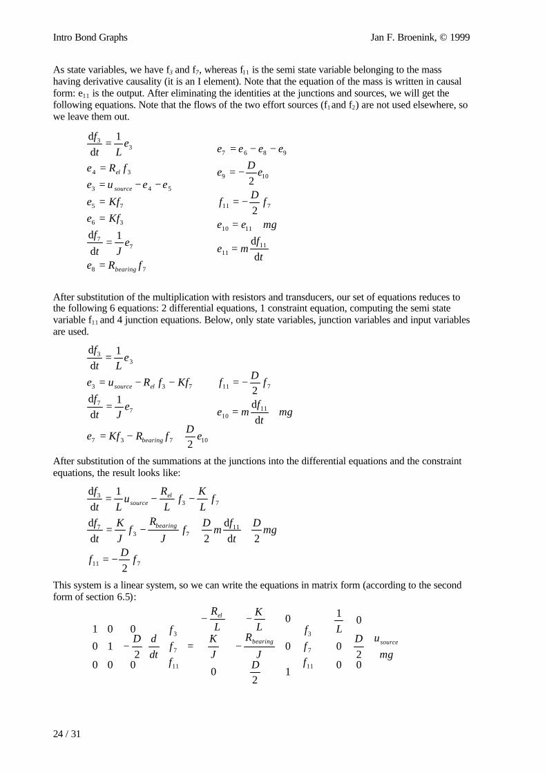
As state variables, we have f3 and f7, whereas f11 is the semi state variable belonging to the masshaving derivative causality (it is an I element). Note that the equation of the mass is written in causalform: e11 is the output. After eliminating the identities at the junctions and sources, we will get thefollowing equations. Note that the flows of the two effort sources (f1 and f2) are not used elsewhere, sowe leave them out.

78

77

36

75

543

34

33

1dd

1dd

fRe

eJt

fKfeKfe

eeuefRe

eLt

f

bearing

source

el

=

=

==

−−==

=

tf

me

mgee

fD

f

eD

e

eeee

dd

2

2

1111

1110

711

109

9867

=

+=

−=

−=

−−=

After substitution of the multiplication with resistors and transducers, our set of equations reduces tothe following 6 equations: 2 differential equations, 1 constraint equation, computing the semi statevariable f11 and 4 junction equations. Below, only state variables, junction variables and input variablesare used.

10737

77

733

33

2

1dd

1dd

eD

fRKfe

eJt

fKffRue

eLt

f

bearing

elsource

+−=

=

−−=

=

mgt

fme

fD

f

+=

−=

dd2

1110

711

After substitution of the summations at the junctions into the differential equations and the constraintequations, the result looks like:

711

1173

7

733

2

2dd

2dd

1dd

fD

f

mgD

tf

mD

fJ

Rf

JK

tf

fLK

fL

Ru

Ltf

bearing

elsource

−=

++−=

−−=

This system is a linear system, so we can write the equations in matrix form (according to the secondform of section 6.5):

+

−

−−

=

−mg

uDL

fff

DJ

R

JK

LK

LR

fff

dtdD sourcebearing

el

002

0

01

12

0

0

0

0002

10

001

11

7

3

11

7

3


25 / 31

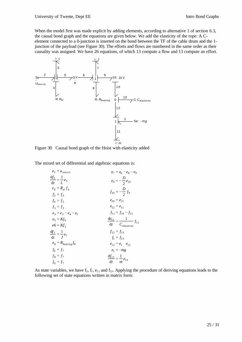
When the model first was made explicit by adding elements, according to alternative 1 of section 6.3,the causal bond graph and the equations are given below. We add the elasticity of the rope: A C-element connected to a 0-junction is inserted on the bond between the TF of the cable drum and the 1-junction of the payload (see Figure 30). The efforts and flows are numbered in the same order as theircausality was assigned. We have 26 equations, of which 13 compute a flow and 13 compute an effort.

Figure 30 Causal bond graph of the Hoist with elasticity added

The mixed set of differential and algebraic equations is:

79

78

76

88

77

5

65

5423

35

34

32

44

33

2

1dd

6

1dd

ffffff

fRe

eJt

f

KfeKfe

eeee

ffffff

fRe

eLt

fue

bearing

el

source

===

=

=

==

−−=

===

=

=

=

1313

1

12113

131

1312

1111

121011

1112

1110

910

109

9867

1d

d

1d

d

2

2

emt

fmge

eeeffff

fCt

efff

eeee

fD

f

eD

e

eeee

elasticity

=

−=

+===

=

−=

==

−=

−=

−−=

As state variables, we have f3, f7, e11 and f13. Applying the procedure of deriving equations leads to thefollowing set of state equations written in matrix form:

I:m

1

R:RbearingR:Rel

Se: -mg1

2

3

4

5 6

7

8

GY1Se

I:L

..K

..Usource

1

I:J

9

10

11

0 C:Celasticity

12

13

TF: /2D


26 / 31

−

+

−−

−−

−−

=

mgu

m

L

feff

m

CCD

DJ

R

JK

LK

Ll

feff

dtd source

elasticityelasticity

bearing

10

0000

01

01

00

0012

02

00Re

13

11

7

3

13

11

7

3

8 Expansion to block diagramsTo show that a causal bond graph is a compact block diagram, we treat in this section the expansion ofa causal bond graph to a block diagram. Furthermore, a block diagram representation of a systemmight be more familiar than a bond graph representation. Thus this work might help understandingbond graphs.

The expansion of a causal bond graph into a block diagram consists of three steps:1. Expand all bonds to bilateral signal flows (two signals with opposite directions). The causal

stroke determines in which direction the effort flows. The bond graph elements can be encircled toconnect the signals to.

2. Replace the bond–graph elements by their block–diagram representations (see section 4). Deducethe signs of the summations of the junctions from the directions of the bond arrows (half arrows,see section 4.5). Often, it is efficient to determine those signs after all bond–graph elements arewritten in block diagram form.The block diagram is ready in principle.

3. Redraw the block diagram in standard form: all integrators in an ongoing stream (form left toright) and all other operations as feedback loops. Of course, this is not always possible. Blocksmight be taken together. Since block diagrams represent mathematical operations, for whichcommutative and associative properties apply, these properties can be used to manipulate theblock diagram such that the result looks appealing enough.

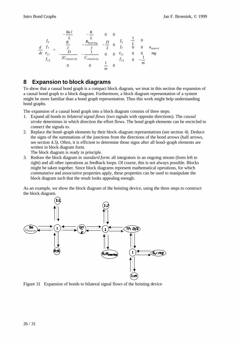
As an example, we show the block diagram of the hoisting device, using the three steps to constructthe block diagram.

Figure 31 Expansion of bonds to bilateral signal flows of the hoisting device

Usource


27 / 31

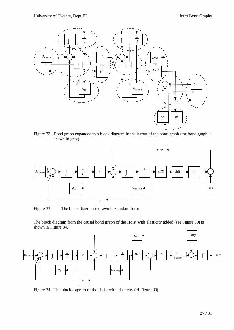
Figure 32 Bond graph expanded to a block diagram in the layout of the bond graph (the bond graph isshown in grey)

Figure 33 The block diagram redrawn in standard form

The block diagram from the causal bond graph of the Hoist with elasticity added (see Figure 30) isshown in Figure 34.

Figure 34 The block diagram of the Hoist with elasticity (cf Figure 30)

∫ ∫∫ ∫

Rel Rbearing

Usource D/2

D/2

1

L

1

JK

K

-mg

1/m1+

--

+-

-

+

-

++

Celasticity

∫ ∫

Rel Rbearing

Usource D/2

D/2

1

L

1

JK

K

-mg

m+

--

+-

-

+ddt

-

I

R R

GY1

1

Se

I I

1 TF

Se

1 1

L J∫ ∫

Usource

Rel Rbearing

D/2

D/2K

K

-mg

mddt

+

-

-+

--

-

-+


28 / 31

9 SimulationThe resulting set of equations coming from a bond–graph model is called the simulation model. Itconsists of first–order ordinary differential equations (ODEs), possibly extended with algebraicconstraint equations (DAEs). Hence, it can be simulated using standard numerical integrationmethods. However, because numerical integration is an approximation of the actual integrationprocess, it is useful to check the simulation model on aspects significant for simulation. As a result, anappropriate integration method can be chosen: the computational work is minimal and the results staywithin a specified error margin.

Since at causal analysis, one can decide whether or not to change the bond–graph model to obtain anexplicit simulation model, it is useful to know about the consequences for simulation of relevantcharacteristics of the simulation model. The following 4 aspects of simulation models are relevant forchoosing an numerical integration method:

1. Presence of implicit equations.Implicit models (DAEs) can only be simulated with implicit integration methods. The iterationprocedure of the implicit integration method is also used to calculate the implicit model. Explicitmodels (ODEs) can be simulated with both explicit as implicit integration methods. Sometimes,implicit integration methods need more computation time than explicit integration methods.During causal analysis, one can see whether a simulation model will be explicit or implicit, seesection 6.3.

2. Presence of discontinuities.Integration methods with special provisions for events will perform best. If that is not available,variable step methods can be used. Multistep methods become less accurate, since they needinformation from the past, which is useless after a discontinuity.While constructing the model, presence of discontinuities can be marked.

3. Numerical stiffness.S(t), the stiffness ratio , is a measure for the distance between real parts of eigenvalues, λ, namelyS(t) = max(|Re(λ(t)|) / min(|Re(λ(t)|). Stiff models (large S) need stiff integration methods. Thetime step is now determined by the stability instead of the accuracy (namely, eigenvalues are nowused to determine the step size). When the high frequency parts are faded out, they do notinfluence the step size anymore. Hence, the step size can grow to limits determined by the lowerfrequencies.

4. Oscillatory parts.When a model has no damping, it should not be simulated with a stiff method. Stiff methodsperform badly for eigenvalues on the imaginary axis (i.e. no damping) of the complex eigenvalueplane.

Eigenvalues can be localised in a causal bond graph, especially when all elements are linear. There isa bond graph version of Mason’s Loop rule to determine the transfer function from a bond graph(Brown, 1972). As a side effect, the eigenvalues can be calculated. We will not discuss the procedureto obtain eigenvalues from a causal bond graph by hand.

10 Conclusion

10.1 ReviewIn this chapter, we have introduced bond graphs to model physical systems in a domain independentway. Only macroscopic systems are treated, thus quantum effects do not play a significant role.Domain indepence has its basics in the fact that physical concepts are analogous for the differentphysical domains. 6 different elementary concepts exist: storage of energy, dissipation, transduction toother domains, distribution, transport, input or output of energy.

Another starting point is that it is possible to write models as directed graphs: parts are interconnectedby bonds, along which exchange of energy occurs. A bond represents the energy flow between the two


29 / 31

connected submodels. This energy flow can be described as the product of 2 variables (effort andflow), letting a bond be conceived as a bilateral signal connection. During modelling, the firstinterpretation is used, while during analysis and equations generation the second interpretation is used.

Furthermore, we presented a method to systematically build a bond graph starting from an idealphysical model. Causal analysis gives, besides the computational direction of the signals at the bonds,also information about the correctness of the model. We presented methods to derive the causality of abond graph. In addition, procedures to generate equations and block diagrams out of a causal bondgraph are presented.

This chapter is only an introduction to bond graphs. Sometimes, procedures are just presented, withouta deep motivation and possible alternatives. It was also not the incentive to elaborate on physicalsystems modelling. We did not discuss multiple connections (arrays of bonds written as onemultibond) and multiport elements (to describe transducers), neither different causal analysisalgorithms. Those different causality algorithms give slightly different sets of DAEs especially whenapplied to certain classes of models (for instance multibody systems with kinematic loops).

10.2 Object-oriented physical-systems modellingNote that bond–graph modelling is in fact a form of object–oriented physical-systems modelling, aterm which is currently often used (Andersson, 1994; Elmqvist et al, 1993; Mattson et al, 1997;Åström et al, 1998). This can be seen as follows: bond–graph models are declarative, can behierarchically structured, and fully support encapsulation (due to the non-causal way of specifyingequations, and the notion of ports). Furthermore, due to allowing hierarchy, the notion of definitionand use of models are distinguished (i.e. the class concept and instantiation). Since bond graphs cameinto existence before the term object oriented was used in the field of physical systems modeling,bond graphs can be seen as an object-oriented physical–systems modeling paradigm avant-la-lettre.

A bond-graph library was written in Modelica (Mattson et al, 1997; Åström et al, 1998) , the upcomingobject-oriented modelling language (Broenink, 1997b). The basic bond–graph elements and block–diagram elements have been specified in Modelica, using the essential object–orientation featuresinheritance and encapsulation. Equations have been specified in an acausal format. Thus, it can besaid that the Modelica modelling concepts are consistent with bond–graph concepts. Furthermore,automatic Modelica code generation from bond graphs appeared to be rather straightforward(Broenink, 1999a).

10.3 Further ReadingFor a more thorough analysis of bond graphs, see Paynter (1961) and Breedveld (1984, 1985), whilean extensive discussion on textbook level is given by Karnopp, Margolis and Rosenberg (1990).Cellier (1991) wrote a textbook on continuous system modelling in which besides bond graphs alsoother modelling methods are used. Current research on bond graphs is reported at the InternationalConference on Bond Graph Modeling, every two years (Granda and Cellier, 1993, 1995, 1997, 1999).Journals regularly publishing bond graph papers are the Journal of the Franklin Institute, which alsohad special issues on bond graphs (1991) and the Journal of Dynamic Systems, Measurement andControl.

11 AcknowledgementsMost of the inspiration for this chapter came from the Dutch course material of Breedveld and VanAmerongen (1994). I sincerely acknowledge Peter Breedveld and Job van Amerongen for theirvaluable suggestions and discussions.

ReferencesAndersson, M., Object–oriented modeling and simulation of hybrid systems, PhD Thesis, Lund

Institute of Technology, Sweden, (1994).


30 / 31

Åström K.J., Elmqvist, H, Mattson, S.E., (1998), Evolution of Continuous–time modeling andsimulation, Proceedings of the 12th European Simulaton Multiconference (ESM’98), SCSPublising, Manchester UK, pp 9-18.

Breedveld P.C. and Amerongen, J. van (1994), Dynamische systemen: modelvorming en simulatie metbondgrafen, (Dynamic systems: modelling and simulation with bond graphs), part 1-4, (inDutch), Dutch Open University, Heerlen, Netherlands, ISBN 90 358 1302 2.

Breedveld P.C., (1982), Thermodynamic Bond Graphs and the problem of Thermal Inertance, Journalof the Franklin Institute, vol 314, no 1, pp. 15-40.

Breedveld P.C., (1984), Physical systems theory in terms of bond graphs, PhD thesis, University ofTwente, Enschede, Netherlands.

Breedveld P.C., (1985), Multibond–graph elements in physical systems theory, Journal of theFranklin Institute , vol 319, no 1/2, pp. 1-36.

Breedveld, P.C. and Dauphin–Tanguy G. (1991), (eds.) Current topics in bond graph related research,Journal of The Franklin Institute, Special issue on bond–graph modeling, Volume 328 no 5/6,Pergamon Press.

Broenink J.F. (1990), Computer–aided Physical–systems modeling and simulation: a bond–graphapproach, PhD thesis, University of Twente, Enschede, Netherlands.

Broenink, J.F. (1997b), Bond–graph modeling in Modelica, Proceedings of 9th European SimulationSymposium, W Hahn, A Lehmann (eds.), Passau Germany, Oct 19-22, pp 137-141.

Broenink, J.F., (1997a), Modelling, Simulation and Analysis with 20-Sim. Journal A, Special issue onCACSD, vol 38 no 3, pp. 22-25, ISSN 0771-1107.

Broenink, J.F. (1999a), Object-oriented modelling with bond graphs and modica. InternationalConference on Bond Graph Modeling ICBGM’99, Simulation Series Vol 31 no 1, SCS, pp. 163-168.

Broenink, J.F., (1999b), 20-SIM, software for hierarchical bond-graph / block-diagram models,Submitted to Journal Simulation in Practice and Theory.

Broenink, J.F., and C. Kleijn, (1999), Computer-aided design of mechatronic systems using 20SIM 3.0,Submitted to WESIC'99, Workshop on Scientific and Industrial Collaboration, Sep 1-3,Newport UK.

Broenink, J.F., Weustink, P.B.T., (1995) PC–version of the bond graph modeling analysis andsimulation tool CAMAS, Proc. International Conference on Bond Graph Modeling ICBGM’95,Simulation Series Vol 27 no 1, SCS, pp. 203-208.

Brown, F.T., (1972), Direct application of the loop rule to bond graphs, Journal of Dynamic Systems,Measurement and Control, Vol 94, no 3, pp253-261.

Cellier F.E., Granda J.J., (1995), (eds.), International Conference on Bond Graph ModelingICBGM’95, Simulation Series Vol 27 no 1, Society for Computer Simulation, San Diego, CA.

Cellier, F.E., (1991) Continuous System Modeling, Springer Verlag, ISBN 0 387 97502 0Dijk, J. van, Breedveld P.C., (1991), Simulation of System Models Containing Zero-order Causal

Paths, J. Franklin Institute 328 (5/6), 959-980Dixhoorn, J.J. van, (1982), Bond graphs and the challenge of a unified modelling theory of physical

systems, Progress in modelling and simulation, Cellier F.E. (ed.), Academic Press, New York,pp 207-245.

Elmqvist, H., Cellier, F.E., and Otter, M. (1993) Object–oriented modeling of hybrid systems, Proc.European Simulation Symposium, Delft, Netherlands, 31-41, (1993).

Granda J.J., (1985), Computer generation of physical system differential equations using bond graphs,Journal of the Franklin Institute, vol 319, no 1/2, pp 243-256.

Granda J.J., Cellier F.E., (1993), (eds.), International Conference on Bond Graph ModelingICBGM’93, Simulation Series Vol 25 no 2, Society for Computer Simulation, San Diego, CA.

Granda J.J., Cellier F.E., (1999), (eds.), International Conference on Bond Graph ModelingICBGM’99, Simulation Series, Vol 31, Society for Computer Simulation, San Diego, CA.

Granda J.J., Dauphin-Tanguy G., (1997), (eds.), International Conference on Bond Graph ModelingICBGM’97, Simulation Series Vol 29 no 1, Society for Computer Simulation, San Diego, CA.

Karnopp D.C., and Rosenberg R.C., (1968), Analysis and Simulation of Multiport Systems – The bondgraph approach to physical system dynamics, MIT Press, Cambridge MA.


31 / 31

Karnopp D.C., and Rosenberg R.C., (1975), System dynamics, a unified approach, J Wiley, NewYork, NY.

Karnopp D.C., Margolis D.L., and Rosenberg R.C., (1990), System dynamics, a unified approach,(2nd edition), J Wiley, New York, NY, ISBN 0 471 45940 2. (Textbook, a teacher’s guide isalso available).

Kron G., (1963), Diakoptics: The piecewise Solution of large–scale systems, Macdonald & Co. Ltd.,London.

Lorenz F., (1997), Modelling System 1, users manual, Lorenz Simulation, Liege, BelgiumMattson, S.E., Elmqvist, H., and Broenink, J.F., (1997), Modelica: An international effort to design the

next generation modeling language, Journal A, Special Issue CACSD, vol 38 (3), pp 22-25.Paynter, H.M. (1961), Analysis and design of engineering systems, MIT Press, Cambridge, MA.Rosenberg R.C., Karnopp D.C., (1983), Introduction to physical system dynamics, McGraw Hill, New

York, NY.Rosenberg, R.C. (1974), A user’s guide to ENPORT–4, Wiley, New York.Thoma, J.U. (1975), Introduction to bond graphs and their applications, Pergamon Press, Oxford.Thoma, J.U. (1989) Simulation by bond graphs - Introduction to a graphical method, Springer Verlag.

introduction to physical systems modelling with bond graphs

Documents

bondgraph submodels

bond graphs canbe

bond graph method

concept of bond graphs

foundations of bond

bond graphsjan

objects bondgraph modelling

bondgraph model description