introduction to principal component...
TRANSCRIPT
Introduction to Principal Component Analysis
Timothy DelSole
George Mason University, Fairfax, Va andCenter for Ocean-Land-Atmosphere Studies, Calverton, MD
July 29, 2010

Other (Equivalent) Names
I Principal component analysis (PCA) (statistics)
I Empirical orthogonal function (EOF) analysis (climate science)
I Karhunen-Loeve Transform (physics, continuous problems)
I Hotelling transform
I Proper orthogonal decomposition (POD) (turbulence).

Climate Studies Involve Large Amounts of Data
Consider a data set Ynm:
n : time step.
m : spatial structure parameter (usually grid point value).
In typical climate studies, m has over 10,000 values(e.g., all elements in a 2.5◦ × 2.5◦ gridded map).
Also, n has 30-3000 values (e.g., annual means or seasonal means).
Space-time climate data can easily exceed one million numbers.
Data Compresion
y
c
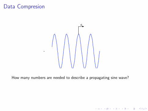
How many numbers are needed to describe a propagating sine wave?
Infinity– sine wave is continuous
Is there a more efficient way to describe a propagating sine wave?
YES: y = A sin(kx − ωt); this requires 3 parameters: A, k, ω.

Data Compresion
y
c
How many numbers are needed to describe a propagating sine wave?
Infinity– sine wave is continuous
Is there a more efficient way to describe a propagating sine wave?
YES: y = A sin(kx − ωt); this requires 3 parameters: A, k, ω.

Data Compresion
y
c
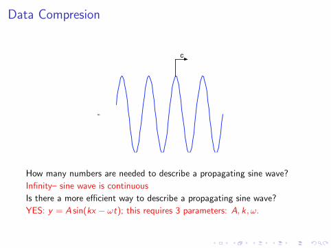
How many numbers are needed to describe a propagating sine wave?
Infinity– sine wave is continuous
Is there a more efficient way to describe a propagating sine wave?
YES: y = A sin(kx − ωt); this requires 3 parameters: A, k, ω.
Data Compresion
y
c
How many numbers are needed to describe a propagating sine wave?
Infinity– sine wave is continuous
Is there a more efficient way to describe a propagating sine wave?
YES: y = A sin(kx − ωt); this requires 3 parameters: A, k, ω.

General Space-Time Decomposition
Any propagating or standing pattern can be described by a sum offixed patterns with time-varying coefficients.
For a propagating sine wave:
sin(kx − ωt) = sin(kx) cos(ωt)− sin(ωt) cos(kx)
More generally:
y(x , y , z , t) = u1(t)v1(x , y , z)+u2(t)v2(x , y , z)+· · ·+uM(t)vM(x , y , z)
Decomposing Climate Data
We would like to reduce the number of numbers needed todescribe a data set.
We will do this by representing the data in the form
Ynm = s1u1nv
1m + s2u2
nv2m + . . . sKuK
n vKm ,
using only a “small” value of K , where
uin defines time variability for the ith component
v im defines spatial structure for the ith component
s i defines the amplitude for the ith component
What is the most efficient set of functions u1n, . . . , u
Kn , v
1m, . . . , v
Km
for approximating Ynm?

Principal Component Analysis
Principal component analysis is a procedure for determining themost efficient approximation of the form
Ynm ≈ s1u1nv
1m + s2u2
nv2m + · · ·+ sKuK
n vKm ,
where “efficient” is defined as minimizing the “distance” betweenthe data and the summed components:∑
n
∑m
(Ynm − s1u1
nv1m − s2u2
nv2m − · · · − sKuK
n vKm
)2.
If the data is exactly represented by K components, then thisprocedure will find it (e.g., K = 2 for a propagating sine wave)

Subtract the Climatological Mean
We often are interested in variability about climatological mean.
Accordingly, we subtract out the climatological mean beforedecomposing data:
Y ′nm = Ynm − Y cnm,
where Y cnm is climatological mean at the nth step and mth variable.
Y′ is often called anomaly data.
If data consists of monthly means, each column of Yc might bethe calendar month mean of the corresponding column of Y.
In long term climate studies, a more appropriate “climatology”might be the mean during a reference “base period.”

Minimization Problem is Ill-PosedWe want to determine the functions u1
n, . . . , uKn , v
1m, . . . , v
Km that
minimizes the “distance” to Ynm.
The “distance” is measured by∑n
∑m
(Ynm − s1u1
nv1m − s2u2
nv2m − · · · − sKuK
n vKm
)2.
Distance depends only on products of the form uinv
im. The same product
can be produced by very different values of uin and v i
m.
This fact implies that the components we seek are not unique.
For instance, uin and v i
m and be multiplied and divided, respectively, bythe same factor and still preserve the product.
Traditionally, this ill-posedness is removed (almost) by imposing that the“lengths” of the components equal one; that is, imposing∑
n
(ui
n
)2= 1 and
∑m
(v im
)2= 1

Matrix Statement of the Problem
The sum of components can be written in matrix form as
s1u1nv
1m + s2u2
nv2m + · · ·+ sKuK
n vKm =⇒ USVT
where
U = [u1 u2 . . . uK ]
V = [v1 v2 . . . vK ]
S = diag [s1 s2 . . . sK ]
We seek the matrices U,V,S that best approximates Y:
Y ≈ USVT
such that (ui )T ui = 1 and (vi )T vi = 1 for all i .

Solution: Singular Value DecompositionEvery matrix Y′ can be written in the form
Y′ = U S VT
[N ×M] [N × N] [N ×M] [M ×M]
where U and V are unitary, and S is a diagonal (not necessarily square)matrix with non-negative diagonal elements.
This is called the singular value decomposition of Y. Unitary means
UT U = UUT = I VT V = VVT = I
columns of U: “left singular vectors”
columns of V: “right singular vectors”
diagonal elements of S: “singular values”
By convention, singular values are ordered in decreasing order.
The first K singular vectors minimize the “distance” to Y, in the sense
that no other K components can have a smaller distance to Y.

Singular Value Decomposition in R
y.svd = svd(y) ; # compute SVD of y
u = y.svd$u ; # extract left singular vectors of yv = y.svd$v ; # extract right singular vectors of ys = y.svd$d ; # extract singular values of y

Example: December-January-February 2m Temperaturedim(t2m) = c(nlon*nlat,ntime); # reshape data matrix
t2m.svd = svd(t(t2m)) ; # calculate svd of transposed matrix
v1 = t2m.svd$v[,1] ; # extract leading right singular vector
dim(v1)=c(nlon,nlat) ; # reshape vector for plotting
image.plot(v1,lon,lat,main="SVD of t2m DJF")
−150 −100 −50 0 50 100 150
−50
050
lon
lat
−0.050
−0.045
−0.040
−0.035
−0.030
−0.025
−0.020
−0.015
−0.010
−0.005
0.000
0.005
0.010
0.015
0.020
SVD of t2m DJF
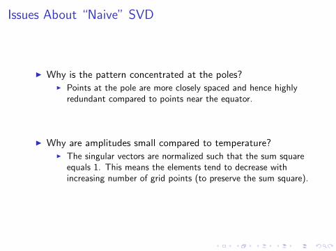
Issues About “Naive” SVD
I Why is the pattern concentrated at the poles?I Points at the pole are more closely spaced and hence highly
redundant compared to points near the equator.
I Why are amplitudes small compared to temperature?I The singular vectors are normalized such that the sum square
equals 1. This means the elements tend to decrease withincreasing number of grid points (to preserve the sum square).
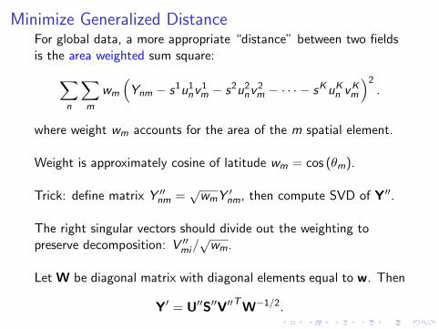
Minimize Generalized DistanceFor global data, a more appropriate “distance” between two fieldsis the area weighted sum square:∑
n
∑m
wm
(Ynm − s1u1
nv1m − s2u2
nv2m − · · · − sKuK
n vKm
)2.
where weight wm accounts for the area of the m spatial element.
Weight is approximately cosine of latitude wm = cos (θm).
Trick: define matrix Y ′′nm =√
wmY ′nm, then compute SVD of Y′′.
The right singular vectors should divide out the weighting topreserve decomposition: V ′′mi/
√wm.
Let W be diagonal matrix with diagonal elements equal to w. Then
Y′ = U′′S′′V′′T
W−1/2.

Area Weighted Principal Component Analysisdim(t2m) = c(nlon*nlat,ntime); # reshape data matrix
weight.area = rep(sqrt(cos(pi*lat/180)),each=nlon); # define weighting
t2m.scaled = (t2m-rowMeans(t2m))*weight.area
t2m.svd = svd(t(t2m.scaled)); # svd of rescaled data
v1 = t2m.svd$v[,1]/weight.area; # extract 1st right singular vector
dim(v1)=c(nlon,nlat) ; # reshape vector for plotting
image.plot(v1,lon,lat)
−150 −100 −50 0 50 100 150
−50
050
lon
lat
−0.05
−0.04
−0.03
−0.02
−0.01
0.00
0.01
0.02
0.03
0.04
0.05
0.06
0.07
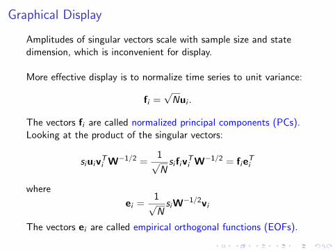
Graphical Display
Amplitudes of singular vectors scale with sample size and statedimension, which is inconvenient for display.
More effective display is to normalize time series to unit variance:
fi =√
Nui .
The vectors fi are called normalized principal components (PCs).Looking at the product of the singular vectors:
siuivTi W−1/2 =
1√N
si fivTi W−1/2 = fie
Ti
where
ei =1√N
siW−1/2vi
The vectors ei are called empirical orthogonal functions (EOFs).
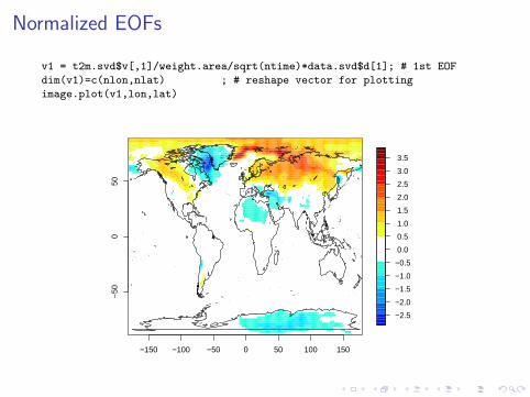
Normalized EOFs
v1 = t2m.svd$v[,1]/weight.area/sqrt(ntime)*data.svd$d[1]; # 1st EOF
dim(v1)=c(nlon,nlat) ; # reshape vector for plotting
image.plot(v1,lon,lat)
−150 −100 −50 0 50 100 150
−50
050
lon
lat
−2.5
−2.0
−1.5
−1.0
−0.5
0.0
0.5
1.0
1.5
2.0
2.5
3.0
3.5

Normalized EOFs
pc1 = t2m.svd$u[,1]*sqrt(ntime); # 1st PC
plot(year,pc1,type="b",col="blue",xlab="year",ylab="",pch=19)
1950 1960 1970 1980 1990 2000
−3
−2
−1
01
year
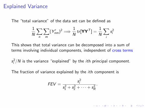
Explained Variance
The “total variance” of the data set can be defined as
1
N
∑n
∑m
(Y ′nm)2 =⇒ 1
Ntr[YYT ] =
1
N
∑i
s2i
This shows that total variance can be decomposed into a sum ofterms involving individual components, independent of cross terms
s2i /N is the variance “explained” by the ith principal component.
The fraction of variance explained by the ith component is
FEV =s2i
s21 + s2
2 + · · ·+ s2R
.
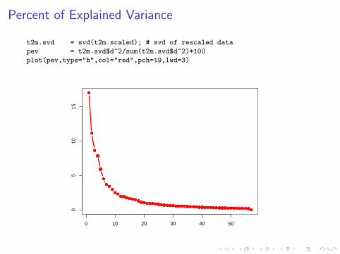
Percent of Explained Variance
t2m.svd = svd(t2m.scaled); # svd of rescaled data
pev = t2m.svd$d^2/sum(t2m.svd$d^2)*100
plot(pev,type="b",col="red",pch=19,lwd=3)
0 10 20 30 40 50
05
1015
Percent of Variance Explained
Index
fev
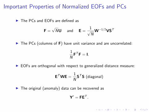
Important Properties of Normalized EOFs and PCs
I The PCs and EOFs are defined as
F =√
NU and E =1√N
W−1/2VST
I The PCs (columns of F) have unit variance and are uncorrelated:
1
NFT F = I.
I EOFs are orthogonal with respect to generalized distance measure:
ET WE =1
NST S (diagonal)
I The original (anomaly) data can be recovered as
Y′ = FET .

Fine Details About Principal Components
I The total number of non-trivial components cannot exceed theminimum of N and M.
I If data is centered, then PCs also are centered.
I If the PCs are known, EOFs can be recovered by projection:
Y′T
F = E.
I If the EOFs are known, PCs can be recovered by projection:
Y′Ei = F where Ei = NWES−2
where “dots” indicate truncated, full rank matrices.
I Ei is the “pseudo-inverse of E and satisfies ET Ei = I.
I EOF vectors ei “explain the most variance,” in that they maximize
var[Y′W−1/2ei ] subject to eTi Wei = 1

Relation to Covariance Matrix
Most texts define principal components as eigenvectors of thecovariance matrix.
The connection can be seen from properties of SVD:
ΣY =1
NYT Y =
1
NVST SVT
This shows that the right singular vectors V also are theeigenvectors of the sample covariance matrix ΣY .
Moreover, the ith eigenvalue λi is related to the singular values as
λi =1
Ns2i
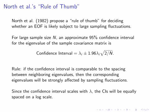
North et al.’s “Rule of Thumb”
North et al. (1982) propose a “rule of thumb” for decidingwhether an EOF is likely subject to large sampling fluctuations.
For large sample size N, an approximate 95% confidence intervalfor the eigenvalue of the sample covariance matrix is
Confidence Interval = λi ± 1.96λi
√2/N.
Rule: if the confidence interval is comparable to the spacingbetween neighboring eigenvalues, then the correspondingeigenvalues will be strongly affected by sampling fluctuations.
Since the confidence interval scales with λ, the CIs will be equallyspaced on a log scale.
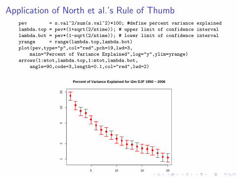
Application of North et al.’s Rule of Thumbpev = s.val^2/sum(s.val^2)*100; #define percent variance explained
lambda.top = pev*(1+sqrt(2/ntime)); # upper limit of confidence interval
lambda.bot = pev*(1-sqrt(2/ntime)); # lower limit of confidence interval
yrange = range(lambda.top,lambda.bot)
plot(pev,type="p",col="red",pch=19,lwd=3,
main="Percent of Variance Explained",log="y",ylim=yrange)
arrows(1:mtot,lambda.top,1:mtot,lambda.bot,
angle=90,code=3,length=0.1,col="red",lwd=2)
5 10 15 20
12
510
20
Index
fev
Percent of Variance Explained for t2m DJF 1950 − 2006

Are EOFs “Dynamical Modes”?
I EOFs are orthogonal, whereas linear modes often are not(especially if derived by linearizing about realistic states).
I “Dynamical Mode” difficult to define for nonlinear systems.
I Linear models generally have neutral modes, which are unrealistic.
I Most realistic linear models are damped and stochastically forced.
I There is only one class of stochastic models whose EOFs correspondto eigenmodes: a linear system with orthogonal eigenmodes drivenby noise that is white in space and time.
I Despite these problems, the leading EOF often resembles the leastdamped mode in linear stochastic models.
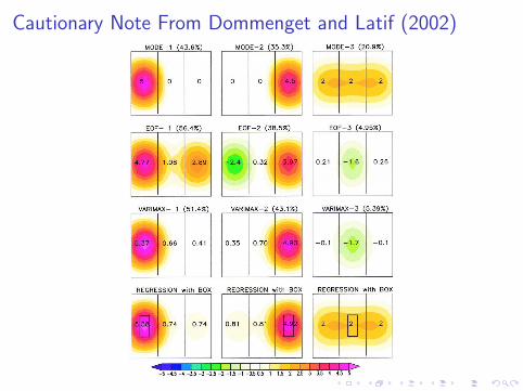
Cautionary Note From Dommenget and Latif (2002)

Is There SOME Procedure That Can Find Modes?Procedures based only on the covariance matrix generally cannotfind modes.
Suppose the modes are the columns of M, and these modesfluctuation with time series T. Then the data is
Y = TMT .
and the covariance matrix is
ΣY =1
NYT Y =
1
NMTT TMT .
Unless there are constraints on the time series T, there is nounique M that yields the covariance matrix ΣY .
For a damped, stochastically forced linear system, modes can beobtained using principal oscillation pattern (POP) analysis, whichrequires time-lagged information.