introduction to probability and statistics eleventh editionvodppl.upm.edu.my/uploads/docs/chapter...

Copyright ©2006 Brooks/Cole

A division of Thomson Learning, Inc.

Introduction to Probability

and Statistics

Twelfth Edition

Robert J. Beaver • Barbara M. Beaver • William Mendenhall

Presentation designed and written by:

Barbara M. Beaver



Introduction to Probability

and Statistics

Twelfth Edition

Chapter 7

Sampling Distributions

Some graphic screen captures from Seeing Statistics ®

Some images © 2001-(current year) www.arttoday.com



Introduction • Parameters are numerical descriptive measures for

populations.

– For the normal distribution, the location and shape

are described by m and s.

– For a binomial distribution consisting of n trials,

the location and shape are determined by p.

• Often the values of parameters that specify the exact

form of a distribution are unknown.

• You must rely on the sample to learn about these

parameters.



Sampling Examples:

• A pollster is sure that the responses to his “agree/disagree” question will follow a binomial distribution, but p, the proportion of those who “agree” in the population, is unknown.

• An agronomist believes that the yield per acre of a variety of wheat is approximately normally distributed, but the mean m and the standard deviation s of the yields are unknown.

If you want the sample to provide reliable information about the population, you must select your sample in a certain way!



Simple Random Sampling

• The sampling plan or experimental design determines the amount of information you can extract, and often allows you to measure the reliability of your inference.

• Simple random sampling is a method of sampling that allows each possible sample of size n an equal probability of being selected.



Example •There are 89 students in a statistics class. The instructor wants to choose 5 students to form a project group. How should he proceed?

1. Give each student a number from 01

to 89.

2. Choose 5 pairs of random digits

from the random number table.

3. If a number between 90 and 00 is

chosen, choose another number.

4. The five students with those

numbers form the group.



Types of Samples

• Sampling can occur in two types of practical

situations:

1. Observational studies: The data existed before you

decided to study it. Watch out for

Nonresponse: Are the responses biased because

only opinionated people responded?

Undercoverage: Are certain segments of the

population systematically excluded?

Wording bias: The question may be too

complicated or poorly worded.



Types of Samples • Sampling can occur in two types of practical

situations:

2. Experimentation: The data are generated by

imposing an experimental condition or treatment on

the experimental units.

Hypothetical populations can make random

sampling difficult if not impossible.

Samples must sometimes be chosen so that the

experimenter believes they are representative of

the whole population.

Samples must behave like random samples!



Other Sampling Plans • There are several other sampling plans that

still involve randomization:

1. Stratified random sample: Divide the population

into subpopulations or strata and select a simple

random sample from each strata.

2. Cluster sample: Divide the population into

subgroups called clusters; select a simple random

sample of clusters and take a census of every element

in the cluster.

3. 1-in-k systematic sample: Randomly select one of

the first k elements in an ordered population, and then

select every k-th element thereafter.



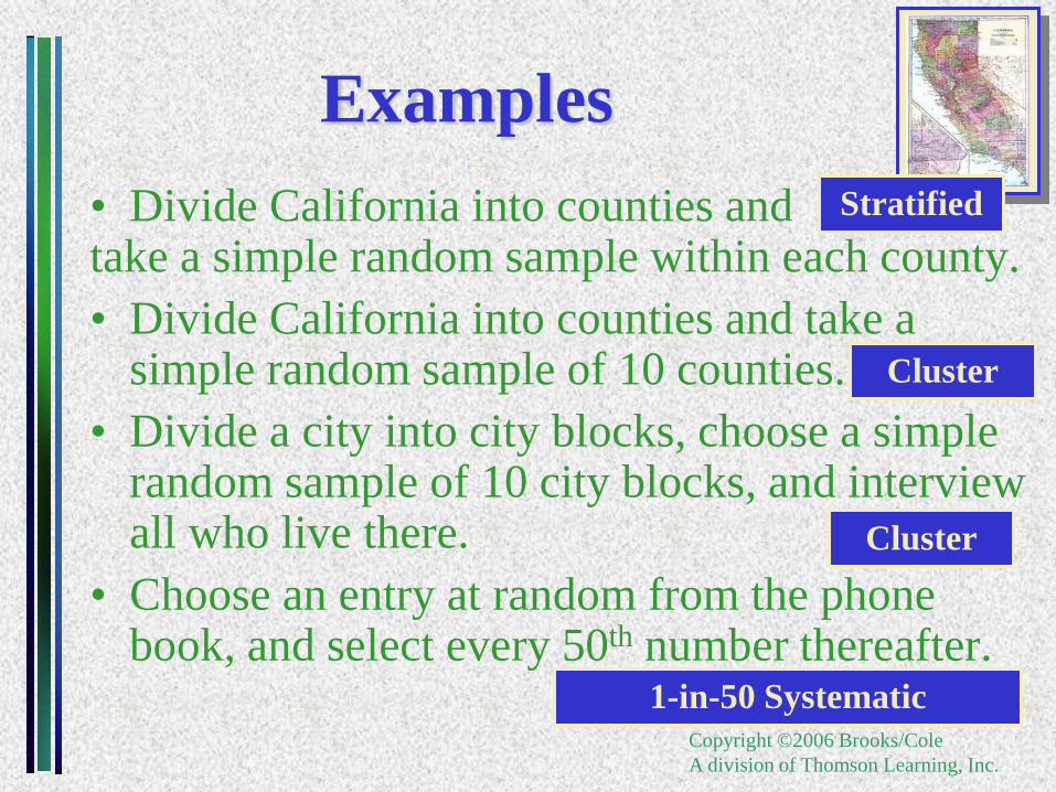
Examples

• Divide California into counties and take a simple random sample within each county.

• Divide California into counties and take a simple random sample of 10 counties.

• Divide a city into city blocks, choose a simple random sample of 10 city blocks, and interview all who live there.

• Choose an entry at random from the phone book, and select every 50th number thereafter.

Cluster

Cluster

1-in-50 Systematic

Stratified



Non-Random Sampling Plans • There are several other sampling plans that

do not involve randomization. They should

NOT be used for statistical inference!

1. Convenience sample: A sample that can be taken easily

without random selection.

• People walking by on the street

2. Judgment sample: The sampler decides who will and won’t

be included in the sample.

3. Quota sample: The makeup of the sample must reflect the

makeup of the population on some selected characteristic.

• Race, ethnic origin, gender, etc.



Sampling Distributions

•Numerical descriptive measures calculated

from the sample are called statistics.

•Statistics vary from sample to sample and

hence are random variables.

•The probability distributions for statistics are

called sampling distributions.

•In repeated sampling, they tell us what values

of the statistics can occur and how often each

value occurs.



Possible samples

3, 5, 2

3, 5, 1

3, 2, 1

5, 2, 1

x

Sampling Distributions Definition: The sampling distribution of a

statistic is the probability distribution for the

possible values of the statistic that results when

random samples of size n are repeatedly drawn

from the population. Population: 3, 5, 2, 1

Draw samples of size n = 3

without replacement

67.23/8

23/6

33/9

33.33/10

Each value of

x-bar is

equally

likely, with

probability

1/4

x

p(x)

1/4

2 3



The characteristics of the

sampling distribution of a statistic

• The distribution of values is obtained

by means of repeated sampling

• The samples are all of size n

• The samples are drawn from the same

population



Central Limit Theorem: If random samples of n

observations are drawn from a nonnormal population with

finite m and standard deviation s , then, when n is large, the

sampling distribution of the sample mean is approximately

normally distributed, with mean m and standard deviation

. The approximation becomes more accurate as n

becomes large.

x

n/s

Sampling Distributions Sampling distributions for statistics can be

Approximated with simulation techniques

Derived using mathematical theorems

- The Central Limit Theorem is one such

theorem.



Example

Toss a balanced die n = 1 time. The distribution of x

the number on the upper face is flat or uniform.

71.1)()(

5.3)6

1(6...)

6

1(2)

6

1(1

)(

2

xpx

xxp

ms

m

APPLET MY

Beaver/diceCLT.html



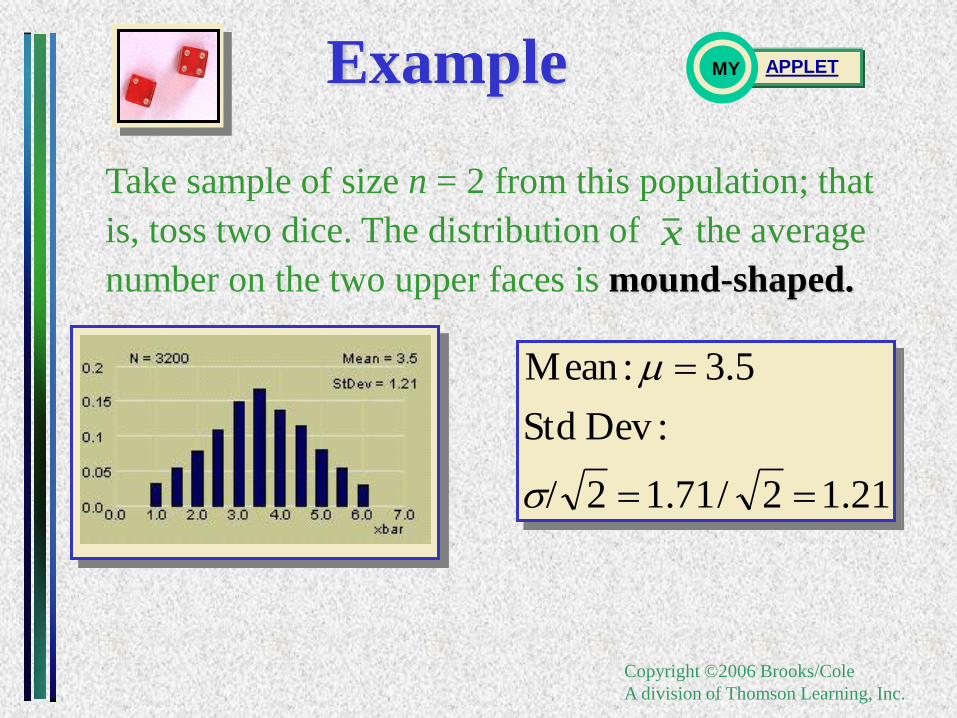
Example

Take sample of size n = 2 from this population; that

is, toss two dice. The distribution of the average

number on the two upper faces is mound-shaped.

21.12/71.12/

:Dev Std

5.3:Mean

s

m

APPLET MY

x

Beaver/diceCLT.html



Example

Using a similar procedure, we generated the

sampling distribution of when n=3. The

sampling distribution of shows a mound shape of

the normal distribution.

987.3/71.13/

:Dev Std

5.3:Mean

s

m

APPLET MY

x

x

Beaver/diceCLT.html



Why is this Important?

The Central Limit Theorem also implies that the

sum of n measurements is approximately normal with

mean m and standard deviation .

Many statistics that are used for statistical inference

are sums or averages of sample measurements.

When n is large, these statistics will have

approximately normal distributions.

This will allow us to describe their behavior and

evaluate the reliability of our inferences.

n/s



How Large is Large? If the sample is normal, then the sampling

distribution of will also be normal, no matter

what the sample size.

When the sample population is approximately

symmetric, the distribution becomes approximately

normal for relatively small values of n.

When the sample population is skewed, the sample

size must be at least 30 before the sampling

distribution of becomes approximately normal.

x

x



n/sx

The Sampling Distribution of

the Sample Mean

A random sample of size n is selected from a

population with mean m and standard deviation s.

The sampling distribution of the sample mean will

have mean m and standard deviation .

If the original population is normal, the sampling

distribution will be normal for any sample size.

If the original population is nonnormal, the sampling

distribution will be normal when n is large.

The standard deviation of x-bar is sometimes called the

STANDARD ERROR (SE).



Exercise



Finding Probabilities for

the Sample Mean

1587.8413.1)1(

)16/8

1012()12(

zP

zPxP

If the sampling distribution of is normal or

approximately normal, standardize or rescale the

interval of interest in terms of

Find the appropriate area using Table 3.

x

n

xz

/s

m

Example: A random

sample of size n = 16

from a normal

distribution with m = 10

and s = 8.



Example A soda filling machine is supposed to fill cans of

soda with 12 fluid ounces. Suppose that the fills are

actually normally distributed with a mean of 12.1 oz

and a standard deviation of .2 oz. What is the

probability that the average fill for a 6-pack of soda is

less than 12 oz?

)12(xP

)6/2.

1.1212

/(

n

xP

s

m

1112.)22.1( zP

APPLET MY

Beaver/zMean.html



Exercise The time that the laptop’s battery pack can

function before recharging is needed is

normally distributed with a mean of 6 hours

and standard deviation of 1.8 hours. A

random sample of 25 laptops with a type of

battery pack is selected and tested. What is

the probability that the mean until recharging

is needed is at least 7 hours?



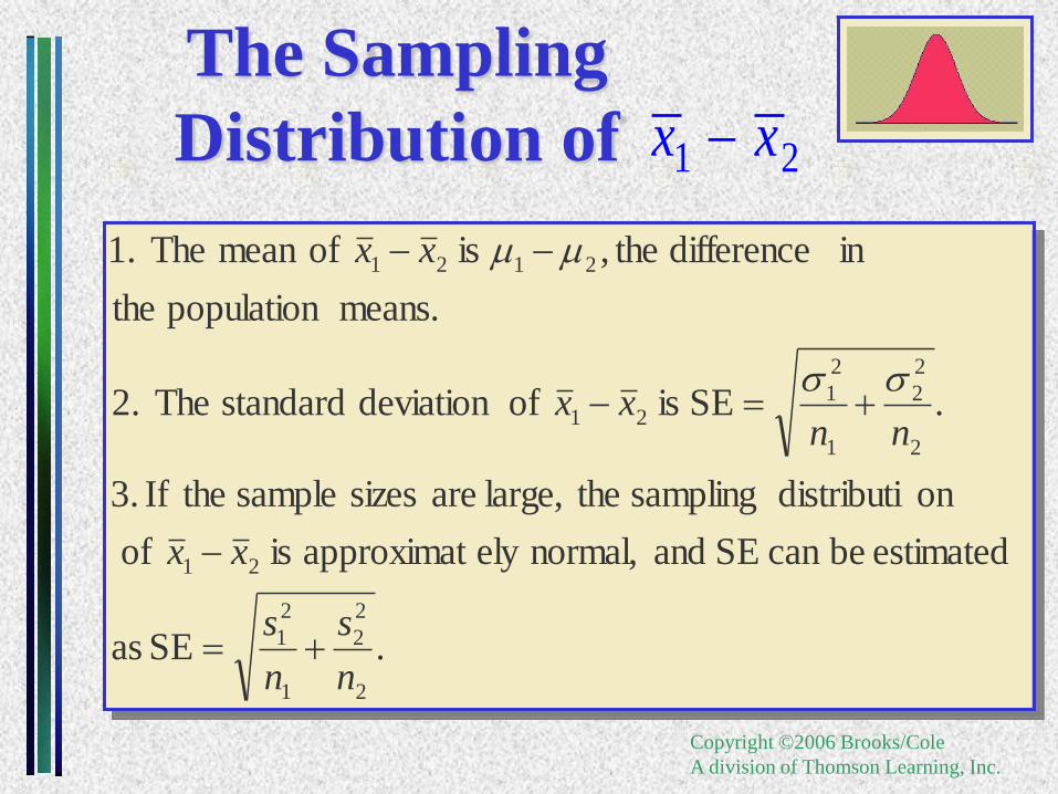
The Sampling

Distribution of 1 2x x

.SE as

estimated becan SE and normal,ely approximat is of

ondistributi sampling thelarge, are sizes sample theIf .3

.SE is ofdeviation standard The 2.

means. population the

in difference the, is ofmean The 1.

2

2

2

1

2

1

21

2

2

2

1

2

121

2121

n

s

n

s

xx

nnxx

xx

ss

mm



Example Starting salaries for MBA graduates at two universities are

normally distributed with the following means and standard

deviations. Samples from each school are taken.

University 1 University 2

Mean RM 62,000 /yr RM 60,000 /yr

Std. Dev. RM14,500 /yr RM18,300 /yr

Sample size, n 50 60

(a) What is the sampling distribution of

(b) What is the probability that a sample mean of University 1

students will exceed the sample mean of University 2

students?



(a) mean:

= 62,000 – 60,000 =2000

standard deviation:

=

= 3128.3

(b)

2 214500 18300

50 60

1 2 1 2x xm m m

Example

1 2

1 2

1 20

1 2

20000 64 1 0 2611 0 7389

3128 3

0 2000

3128 3( )

( . ) . ..

( )

.

x x

x x

P x x P

P z P z

x x m

s



The Sampling Distribution

of the Sample Proportion The Central Limit Theorem can be used to

conclude that the binomial random variable x is

approximately normal when n is large, with mean np

and standard deviation .

The sample proportion, is simply a rescaling

of the binomial random variable x, dividing it by n.

From the Central Limit Theorem, the sampling

distribution of will also be approximately

normal, with a rescaled mean and standard deviation.

n

xp ˆ

p̂



The Sampling Distribution

of the Sample Proportion

The standard deviation of p-hat is sometimes called

the STANDARD ERROR (SE) of p-hat.

A random sample of size n is selected from a

binomial population with parameter p.

The sampling distribution of the sample proportion,

will have mean p and standard deviation

If n is large, and p is not too close to zero or one, the

sampling distribution of will be approximately

normal.

n

xp ˆ

n

pq

p̂



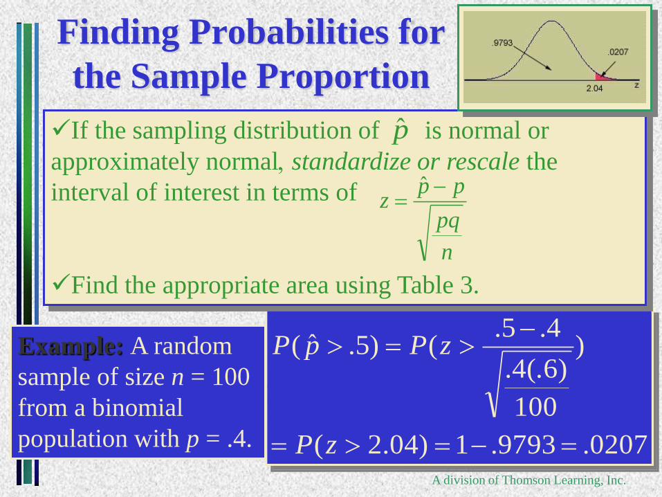
Finding Probabilities for

the Sample Proportion

0207.9793.1)04.2(

)

100

)6(.4.

4.5.()5.ˆ(

zP

zPpP

If the sampling distribution of is normal or

approximately normal, standardize or rescale the

interval of interest in terms of

Find the appropriate area using Table 3.

p̂

n

pq

ppz

ˆ

Example: A random

sample of size n = 100

from a binomial

population with p = .4.



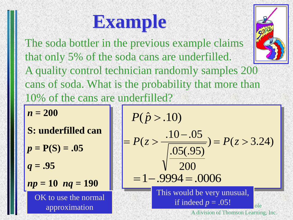
Example The soda bottler in the previous example claims

that only 5% of the soda cans are underfilled.

A quality control technician randomly samples 200

cans of soda. What is the probability that more than

10% of the cans are underfilled?

)10.ˆ( pP

)24.3()

200

)95(.05.

05.10.(

zPzP

0006.9994.1 This would be very unusual,

if indeed p = .05!

n = 200

S: underfilled can

p = P(S) = .05

q = .95

np = 10 nq = 190

OK to use the normal

approximation



The Sampling

Distribution of 1 2ˆ ˆp p

.ˆˆˆˆ

SE as

estimated becan SE and normal,ely approximat is ˆˆ of

ondistributi sampling thelarge, are sizes sample theIf .3

.SE is ˆˆ ofdeviation standard The 2.

s.proportion population the

in difference the, is ˆˆ ofmean The 1.

2

22

1

11

21

2

22

1

1121

2121

n

qp

n

qp

pp

n

qp

n

qppp

pppp



Example It is known that 16% of the households in Community A and 11% of

the households in Community B have internets in their houses. If 200

households from Community A and 225 households from Community

B are selected at random, compute the probability of observing the

difference between the proportion of having internets in the two

samples are at least 0.10.

0 16 0 11 0 05

0 16 0 84 0 11 0 890 033

200 225

0 1 0 050 1

0 033

1 52 1 0 9357 0 0643

ˆ ˆ

ˆ ˆ

ˆ ˆ

ˆ ˆ

. . .

( . )( . ) ( . )( . ).

ˆ ˆ( ) . .ˆ ˆ( . )

.

( . ) . .

A B

A B

A B

A B

p p A B

A A B Bp p

A B

A B p p

A B

p p

p p

p q p q

n n

p pP p p P

P z

m

s

m

s



Sampling Distribution of S2

If S2 is the variance of a random sample of size n taken

from a normal population having the variance s2, then the

statistic

has a chi-squared distribution with v = n -1 degrees of

freedom.

Example:

22

2

1( )n S

s

167.2

067.14

7For

2

95.0

2

05.0

v



Key Concepts I. Sampling Plans and Experimental Designs

1. Simple random sampling

a. Each possible sample is equally likely to occur.

b. Use a computer or a table of random numbers.

c. Problems are nonresponse, undercoverage, and

wording bias.

2. Other sampling plans involving randomization

a. Stratified random sampling

b. Cluster sampling

c. Systematic 1-in-k sampling



Key Concepts 3. Nonrandom sampling

a. Convenience sampling

b. Judgment sampling

c. Quota sampling

II. Statistics and Sampling Distributions

1. Sampling distributions describe the possible values of a

statistic and how often they occur in repeated sampling.

2. Sampling distributions can be derived mathematically,

approximated empirically, or found using statistical theorems.

3. The Central Limit Theorem states that sums and averages of

measurements from a nonnormal population with finite mean

m and standard deviation s have approximately normal

distributions for large samples of size n.



Key Concepts III. Sampling Distribution of the Sample Mean

1. When samples of size n are drawn from a normal population

with mean m and variance s 2, the sample mean has a

normal distribution with mean m and variance s 2/n.

2. When samples of size n are drawn from a nonnormal

population with mean m and variance s 2, the Central Limit

Theorem ensures that the sample mean will have an

approximately normal distribution with mean m and variance

s 2 /n when n is large (n 30).

3. Probabilities involving the sample mean m can be calculated

by standardizing the value of using n

xz

/s

m

x

x

x



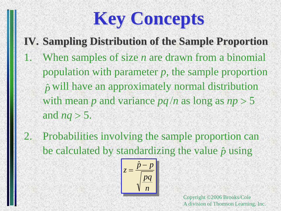
Key Concepts IV. Sampling Distribution of the Sample Proportion

1. When samples of size n are drawn from a binomial

population with parameter p, the sample proportion

will have an approximately normal distribution

with mean p and variance pq /n as long as np 5

and nq 5.

2. Probabilities involving the sample proportion can

be calculated by standardizing the value using

n

pq

ppz

ˆ

p̂

p̂

introduction to probability and statistics eleventh editionvodppl.upm.edu.my/uploads/docs/chapter...

Documents