introduction to programming concepts with case studies in python || managing the size of a problem

Chapter 4Managing the Size of a Problem

As explained in Chap. 3, programming is all about world problems. Sometimes, aprogrammer needs to deal with program demands for

• converting Celsius degree to Fahrenheit degree for the expected temperature inParis tomorrow,

• solving a quadratic equation for an unknown x,• calculating the edge lengths of a rectangle given the coordinates of the lower-left

and upper-right corners.

These tasks are ‘tiny’ in the sense that the required programming is merely aboutcalculation of a few expressions.

However, there are times when the demand is somehow different. For example,consider the case that the degree conversion is about all the cities in the world foreach month of the year for the past 20 years. This now is a different case whichrequires a large amount of computation to be undertaken.

In contrast to ‘tiny’, we call such problems ‘bulky’; these are problems where youcan talk about the ‘size’ of the problem. Keeping the nature the same but changingthe size, the problem varies from ‘tiny’ to ‘bulky’.

We tackle such problems with two techniques: ‘recursion’, the most powerfulweapon of the functional programming paradigm and the ‘iteration’ construct ofthe imperative paradigm. Interestingly, recursion is elegant, easier to understand butmore difficult to build up. On the other hand, iteration is quick and dirty, easierto construct but more difficult to understand within an already written code. Afterhaving introduced both techniques, we will discuss and compare both techniques.

4.1 An Action Wizard: Recursion

The recursive-oriented approach is somewhat awkward for human understandingsince we usually do not handle daily problems in a recursive manner. For example,it is quite hard to find a person who would define a postman’s work as a job carriedout on a bag of letters, as follows:

G. Üçoluk, S. Kalkan, Introduction to Programming Concepts with Case Studiesin Python, DOI 10.1007/978-3-7091-1343-1_4, © Springer-Verlag Wien 2012

121

http://dx.doi.org/10.1007/978-3-7091-1343-1_4

122 4 Managing the Size of a Problem

Job(bag_of_letters) is defined as

1. If the bag is empty, do nothing.2. else take out and deliver the first letter in the bag.3. Do Job(bag_with_one_letter_less)

However, this type of approach is very helpful in functional programming. There-fore, we had better take a closer look at it. Consider the common definition of fac-torial. Literally, it is defined as:

Except for zero, the factorial of a natural number is defined as the numberobtained by multiplying all the natural numbers (greater than zero) less thanor equal to it. The factorial of zero is defined as 1.

In mathematical notation, this can be written as in Eq. 4.1 (denoting the factorialwith the postfix operator (!)):

N ! = 1 × 2 × · · · × (N − 1) × N N ∈ N,N > 0

0! = 1(4.1)

Equation 4.1 can be neatly put into pseudo-code as:define factorial(n)

acum ← 1while n > 0 do

acum ← acum × n

n ← n − 1return acum

When we investigate the mathematical definition (Eq. 4.1) closer, we recognizethat the first N − 1 terms in the multiplication are nothing else but the (N − 1)!itself:

N ! = 1 × 2 × · · · × (N − 1)︸︷︷︸

(N−1)!×N N ∈ N,N > 0

Therefore, as an alternative to the previous definition, we could define the factorialas in Eq. 4.2:

N ! = (N − 1)! × N N ∈ N,N > 0

0! = 1(4.2)

There is a very fundamental and important difference between the two mathematicaldefinitions (Eqs. 4.1 and 4.2). The later makes use of the ‘defined term’ (the factorialfunction) in the definition itself (on the right hand side of the definition) whereas theformer does not.

Unless such a relation (as in the second definition in Eq. 4.2) boils down to atautology and maintains its logical consistency, it is valid. Such relations are calledrecurrence relations and algorithms which rely on them are called recursive algo-rithms.

4.1 An Action Wizard: Recursion 123

Now, let us have a look at the recursive algorithm (written down in pseudo code)which evaluates the factorial of a natural number:

define factorial(n)

if n?= 0 then

return 1else

return n × factorial(n − 1)

Notice the similarity to the mathematical definition (Eq. 4.2) and the elegance ofthe algorithm.

Recurrence can occur in more complex forms. For example, the evenness andoddness of natural numbers could be recursively defined as:

• 0 is even.• 1 is odd.• A number is even if one less of the number is odd.• A number is odd if one less of the number is even.

This definition is recursive since we made use of the concept which is being definedin the definition. Such definitions are called mutually recursive.

Are all problems suitable to be solved by a recursive approach? Certainly not.The problems that are more suitable for recursion have the following properties:

• ‘Scalable problems’are good candidates to be solved by recursion. The term ‘scal-able’ means that the problem has a dimension in which we are able to talk abouta ‘size’. For example, a problem of calculating the grades of a class with 10 stu-dents is ‘smaller’ in ‘size’ compared to a problem of calculating the grades of aclass with 350 students. Presumably, the reader has already recognized that the‘size’ mentioned above has nothing to do with the ‘programming effort’. In thiscontext, ‘size’ is merely a concept of the ‘computational effort’. For example,assume that you are asked to calculate the grade of a single student, which isobtained through a very complicated algorithmic expression, and that this algo-rithmic expression will cost you a great deal of ‘programming effort’. Now, ifthe algorithmic expression were not so complicated, you would spend less ‘pro-gramming effort’; however, this does not imply that this problem is suitable forrecursive programming.

• A second propertyof a recursively solvable problem is that whether any instanceof the problem is ‘downsizable’ as far as the ‘sizable’ dimension is concerned.This needs some explanation: By removing some entities from the data that rep-resents the sizable dimension of the problem, can we obtain a ‘smaller’ problemof exactly the same type?

• The third propertyis strongly related to the second one. It should be possible to‘construct’ the solution to the problem from the solution(s) of the ‘downsized’problem. The ‘downsized’ problem is generated by removing some data from the‘sizable dimension’ of the original problem and obtaining (at least) one sub-part,which is still of the sizeable dimension’s data type, but now smaller.


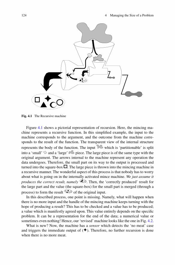
Fig. 4.1 The Recursive machine

Figure 4.1 shows a pictorial representation of recursion. Here, the mincing ma-chine represents a recursive function. In this simplified example, the input to themachine corresponds to the argument, and the outcome from the machine corre-sponds to the result of the function. The transparent view of the internal structure

represents the body of the function. The input which is ‘partitionable’ is splitinto a ‘small’ and a ‘large’ piece. The large piece is of the same type with theoriginal argument. The arrows internal to the machine represent any operation thedata undergoes. Therefore, the small part on its way to the output is processed andturned into the square-box . The large piece is thrown into the mincing machine ina recursive manner. The wonderful aspect of this process is that nobody has to worryabout what is going on in the internally activated mince machine. We just assume itproduces the correct result, namely . Then, the ‘correctly produced’ result forthe large part and the value (the square-box) for the small part is merged (through a

process) to form the result of the original input.In this described process, one point is missing. Namely, what will happen when

there is no more input and the handle of the mincing machine keeps turning with thehope of producing a result? This has to be checked and a value has to be produced;a value which is manifestly agreed upon. This value entirely depends on the specificproblem. It can be a representation for the end of the data; a numerical value orsometimes even nothing! Hence, our ‘revised’ machine looks like the one in Fig. 4.2.

What is new? Now, the machine has a sensor which detects the ‘no meat’ caseand triggers the immediate output of ( ). Therefore, no further recursion is donewhen there is no more meat.


Fig. 4.2 The revised recursive machine

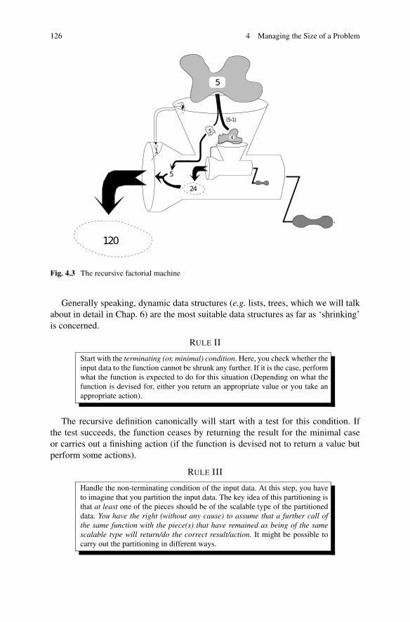
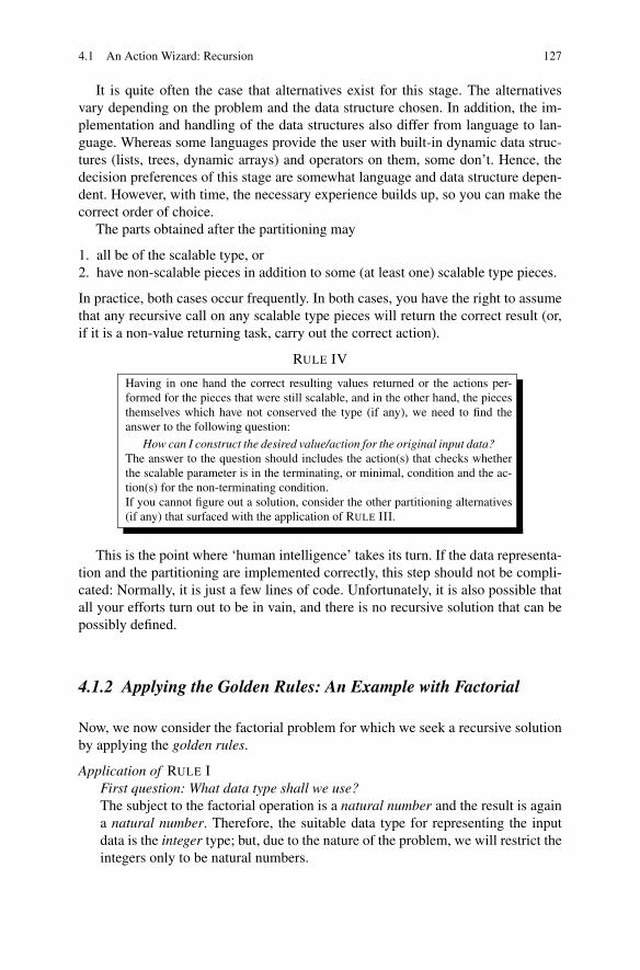
Now the machinery in action: In this particular case, it will mimic the recursivecalculation of the factorial. To be more precise, if ‘the recursive factorial machine’is to calculate 5!, the mincing machine looks like Fig. 4.3.

4.1.1 Four Golden Rules for Brewing Recursive Definitions

RULE I

Look at the (data) content of the problem and decide on a suitable data rep-resentation. The chosen data representation should allow easy shrinking andexpansion with the change in the problem’s data.

For example, if the scalable dimension of the problem is about age, then naturallyyou would decide to use integer as the data type. If it is about a set of human names,then any container of strings would be acceptable. If it is about a sparse graph prob-lem, then maybe a list structure of edge informations would be the best choice. Here,the main principle is to choose a data structure which is easy to shrink in relation tothe downscaling. The string data type is, for example, easy to shrink or grow. On theother hand, arrays are more troublesome. Usually, if an array is chosen for the datarepresentation, the shrinking is not carried out directly on the representation. Thepreferred technique is to keep and update the start and end indexes (integer values)that refer to the actual array.


Fig. 4.3 The recursive factorial machine

Generally speaking, dynamic data structures (e.g. lists, trees, which we will talkabout in detail in Chap. 6) are the most suitable data structures as far as ‘shrinking’is concerned.

RULE II

Start with the terminating (or, minimal) condition. Here, you check whether theinput data to the function cannot be shrunk any further. If it is the case, performwhat the function is expected to do for this situation (Depending on what thefunction is devised for, either you return an appropriate value or you take anappropriate action).

The recursive definition canonically will start with a test for this condition. Ifthe test succeeds, the function ceases by returning the result for the minimal caseor carries out a finishing action (if the function is devised not to return a value butperform some actions).

RULE III

Handle the non-terminating condition of the input data. At this step, you haveto imagine that you partition the input data. The key idea of this partitioning isthat at least one of the pieces should be of the scalable type of the partitioneddata. You have the right (without any cause) to assume that a further call ofthe same function with the piece(s) that have remained as being of the samescalable type will return/do the correct result/action. It might be possible tocarry out the partitioning in different ways.


It is quite often the case that alternatives exist for this stage. The alternativesvary depending on the problem and the data structure chosen. In addition, the im-plementation and handling of the data structures also differ from language to lan-guage. Whereas some languages provide the user with built-in dynamic data struc-tures (lists, trees, dynamic arrays) and operators on them, some don’t. Hence, thedecision preferences of this stage are somewhat language and data structure depen-dent. However, with time, the necessary experience builds up, so you can make thecorrect order of choice.

The parts obtained after the partitioning may

1. all be of the scalable type, or2. have non-scalable pieces in addition to some (at least one) scalable type pieces.

In practice, both cases occur frequently. In both cases, you have the right to assumethat any recursive call on any scalable type pieces will return the correct result (or,if it is a non-value returning task, carry out the correct action).

RULE IV

Having in one hand the correct resulting values returned or the actions per-formed for the pieces that were still scalable, and in the other hand, the piecesthemselves which have not conserved the type (if any), we need to find theanswer to the following question:

How can I construct the desired value/action for the original input data?The answer to the question should includes the action(s) that checks whetherthe scalable parameter is in the terminating, or minimal, condition and the ac-tion(s) for the non-terminating condition.If you cannot figure out a solution, consider the other partitioning alternatives(if any) that surfaced with the application of RULE III.

This is the point where ‘human intelligence’ takes its turn. If the data representa-tion and the partitioning are implemented correctly, this step should not be compli-cated: Normally, it is just a few lines of code. Unfortunately, it is also possible thatall your efforts turn out to be in vain, and there is no recursive solution that can bepossibly defined.

4.1.2 Applying the Golden Rules: An Example with Factorial

Now, we now consider the factorial problem for which we seek a recursive solutionby applying the golden rules.

Application of RULE IFirst question: What data type shall we use?The subject to the factorial operation is a natural number and the result is againa natural number. Therefore, the suitable data type for representing the inputdata is the integer type; but, due to the nature of the problem, we will restrict theintegers only to be natural numbers.


Second question: Is this data type partitionable in the terms explained above?Yes, indeed. There exist operations like subtraction and division defined overthe integers which produce smaller pieces (in this case, all of the integer typesas well).

Application of RULE IIHaving decided on the data type (integer in this case), now we need to deter-mine the terminating condition. We know that the smallest integer the facto-rial function would allow as an argument is 0, and the value to be returnedfor this input value is 1. Therefore, we have the following terminating condi-tion:define factorial(n)

if n?= 0 then

return 1else

. . .Application of RULE III

The question is: How can we partition the argument (in this case n), so that atleast one of the pieces remains an integer?Actually, there are many ways to do it. Before presenting the result, here westate some first thoughts (some of which will turn out to be useless).

Partitionings where all the pieces are of the same type

• For example, we can partition our number n in half; namely into twonearly equal pieces n1 and n2 so that either n1 = n2 or n1 = n2 + 1. Cer-tainly, it is true that each of the ‘pieces’ n1 and n2 is ‘smaller’ than n,the actual argument. Furthermore, each of the pieces remain as the sametype of n; in other words, they are all of an integer type and hence, it ispossible to pass them to the factorial function (actually, RULE II says thatit is sufficient if one of the pieces is an integer type; here, we have all ofthem satisfying this property).

• Alternatively, for example, it is possible to partition n into its additive con-stituents so that n = n1 +n2 +· · ·+nk . There are many ways to make thispartition and as it was for the factors above, each ni will remain smallerthan n and each one will satisfy the property of being an integer. There-fore, it is possible to pass them to the factorial function as an argument.

Partitionings with one ‘small’ piece and a ‘large’ pieceFor example,

• n can be additively split into a large piece: n − 1 and a small piece: 1.• n can be additively split into a large piece: n−2 and a small piece: 2 (This

will require n ≥ 2).

• ...

Due to the nature of the results of those integer operations, all the pieces(including the small ones) will possess the property of ‘being the same type


as the argument of the factorial function’, namely the integer type, but infact, this is not our concern: we require this condition to be met only for thelarge pieces.

Application of RULE IVNow, we have various ways of partitioning the input data n and of course, theinput argument n itself. For every partitioning scheme, we have the right to makethe very important assumption that

A further call of the factorial function with the ‘pieces’ that preserved thetype (i.e., positive integer) will produce the correct result.

Certainly, we will not trace all the thought experimentations related to everyway of partitioning. However, as an example, consider the n = n1 + n2 partitionwhere n1 differs from n2 by 1 at the most. Due to the ‘right of assumption’(stated above), we can assume that n1! and n2! are both known. The questionthat follows is:

Given n, n1, n2, n1!, n2! can we compute n! in an easy manner?

Take your time, think about it; but, you will discover that there is no easy way toobtain n! from these constituents. Except for one of the partitions, all will turnout to be useless. The only useful one is the additive partitioning of n as n − 1and 1. Considering also the ‘right of assumption’, we have at hand

• n

• 1• n − 1• 1!• (n − 1)!It is, as a human being, your duty to discover (or know) the fact that

n! = n × (n − 1)!

And, there you have the solution. (Some readers may wonder why we have notused all that we have at hand. It is true that we have not and there is nothingwrong with that. Those are the possible ingredients that you are able to use. Tohave the ability to use them does not necessarily mean that you have to use themall. In this case, the use of n and (n − 1)! suffices.)For the sake of completeness, let us write the complete algorithm:

define factorial(n)

if n?= 0 then

return 1else

return n × factorial(n − 1)


4.1.3 Applying the Golden Rules: An Example with List Reversal

The second example that we will consider is the problem of reversing a given list. Ifthe desired function is named reverse, we expect to obtain the result [y,n,n,u,f ]from calling reverse([f,u,n,n, y]).

We assume that head and tail operations are defined for lists which respectivelycorrespond to the first item of the list and all items but the first item of the list; inother words, head([f,u,n,n, y]) = f and tail([f,u,n,n, y]) = [u,n,n, y]. More-over, we assume that we have a tool which does the inverse of this operation (i.e.,given the head and the tail of a list, it combines them into one list). Therefore, itseems to be quite logical to put the list (in our example [f,u,n,n, y]) into twopieces; namely, its head: f and tail: [u,n,n, y]. Is GOLDEN RULE III satisfied?Yes, indeed. The tail is still of the list type. The same rule says that if we havesatisfied this criterion, then we have the right to assume that a recursive call withthe tail as argument will yield the correct result. Therefore, we have the right to as-sume that the recursive call reverse(tail([f,u,n,n, y])) will return the correct result[y,n,n,u]. Now, let us look at what we have in our inventory:

• [f,u,n,n, y] the argument• f the head of the argument• [u,n,n, y] the tail of the argument• [y,n,n,u] result of a recursive call with the tail as argument

GOLDEN RULE IV says that we should look for an easy way that will generatethe correct result using the entities in the inventory. We observe that the desiredoutcome of [y,n,n,u,f ] is easily obtained by the operation

[u,n,n, y]︸︷︷︸

tail([f,u,n,n,y])· [ f

︸︷︷︸

head([f,u,n,n,y])]

also taking into account the trivial case of an empty set (which fulfills the require-ment of RULE II), we are able to write the full definition (⊕ denotes list concatena-tion):

define reverse(S)

if S?= ∅ then

return ∅else

return reverse(tail(S)) ⊕ [head(S)]

4.1.4 A Word of Caution About Recursion

Recursive solutions are so elegant that sometimes we can miss unnecessary invoca-tions of recursion and can re-compute what have already been computed.


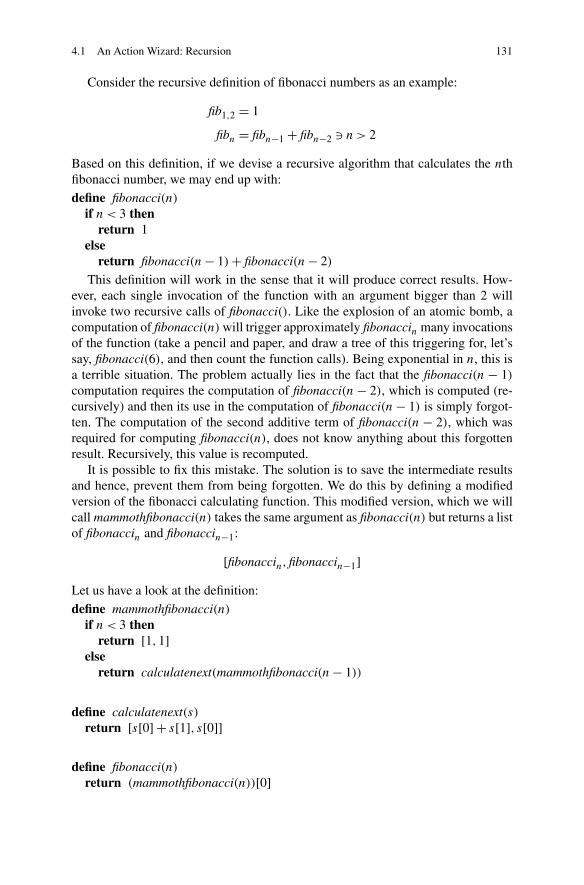
Consider the recursive definition of fibonacci numbers as an example:

fib1,2 = 1

fibn = fibn−1 + fibn−2 � n > 2

Based on this definition, if we devise a recursive algorithm that calculates the nthfibonacci number, we may end up with:define fibonacci(n)

if n < 3 thenreturn 1

elsereturn fibonacci(n − 1) + fibonacci(n − 2)

This definition will work in the sense that it will produce correct results. How-ever, each single invocation of the function with an argument bigger than 2 willinvoke two recursive calls of fibonacci(). Like the explosion of an atomic bomb, acomputation of fibonacci(n) will trigger approximately fibonaccin many invocationsof the function (take a pencil and paper, and draw a tree of this triggering for, let’ssay, fibonacci(6), and then count the function calls). Being exponential in n, this isa terrible situation. The problem actually lies in the fact that the fibonacci(n − 1)

computation requires the computation of fibonacci(n − 2), which is computed (re-cursively) and then its use in the computation of fibonacci(n − 1) is simply forgot-ten. The computation of the second additive term of fibonacci(n − 2), which wasrequired for computing fibonacci(n), does not know anything about this forgottenresult. Recursively, this value is recomputed.

It is possible to fix this mistake. The solution is to save the intermediate resultsand hence, prevent them from being forgotten. We do this by defining a modifiedversion of the fibonacci calculating function. This modified version, which we willcall mammothfibonacci(n) takes the same argument as fibonacci(n) but returns a listof fibonaccin and fibonaccin−1:

[fibonaccin,fibonaccin−1]Let us have a look at the definition:

define mammothfibonacci(n)

if n < 3 thenreturn [1,1]

elsereturn calculatenext(mammothfibonacci(n − 1))

define calculatenext(s)return [s[0] + s[1], s[0]]

define fibonacci(n)

return (mammothfibonacci(n))[0]


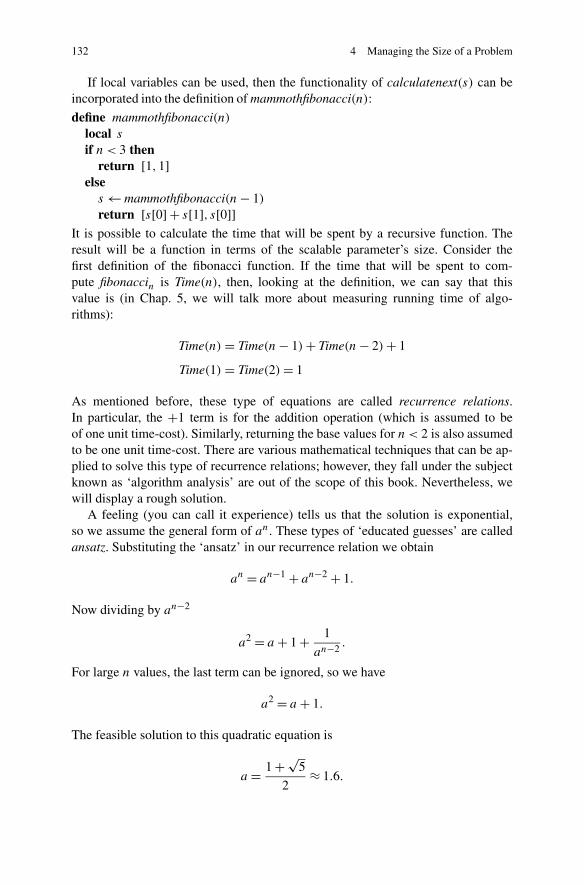
If local variables can be used, then the functionality of calculatenext(s) can beincorporated into the definition of mammothfibonacci(n):

define mammothfibonacci(n)

local s

if n < 3 thenreturn [1,1]

elses ← mammothfibonacci(n − 1)

return [s[0] + s[1], s[0]]It is possible to calculate the time that will be spent by a recursive function. Theresult will be a function in terms of the scalable parameter’s size. Consider thefirst definition of the fibonacci function. If the time that will be spent to com-pute fibonaccin is Time(n), then, looking at the definition, we can say that thisvalue is (in Chap. 5, we will talk more about measuring running time of algo-rithms):

Time(n) = Time(n − 1) + Time(n − 2) + 1

Time(1) = Time(2) = 1

As mentioned before, these type of equations are called recurrence relations.In particular, the +1 term is for the addition operation (which is assumed to beof one unit time-cost). Similarly, returning the base values for n < 2 is also assumedto be one unit time-cost. There are various mathematical techniques that can be ap-plied to solve this type of recurrence relations; however, they fall under the subjectknown as ‘algorithm analysis’ are out of the scope of this book. Nevertheless, wewill display a rough solution.

A feeling (you can call it experience) tells us that the solution is exponential,so we assume the general form of an. These types of ‘educated guesses’ are calledansatz. Substituting the ‘ansatz’ in our recurrence relation we obtain

an = an−1 + an−2 + 1.

Now dividing by an−2

a2 = a + 1 + 1

an−2.

For large n values, the last term can be ignored, so we have

a2 = a + 1.

The feasible solution to this quadratic equation is

a = 1 + √5

2≈ 1.6.


Therefore, the result is

Time(n) ∝ (1.6)n.

A similar analysis for the corrected form (the one with mammothfibonacci) yields

Time(n) ∝ n.

4.1.5 Recursion in Python

In Python, you can implement recursive functions. Since there is no syntac-tic or semantic difference to calling a different function, we will just illustraterecursion in Python with several examples.

– Factorial of a Number

Similar to writing a “Hello World” program at the beginning of learning a newprogramming language, it is common to illustrate recursion using the factorialof a number. Remember that n! equals n×(n−1)×(n−2)×· · ·×1, which canbe re-written as n× (n− 1)!. Below is the corresponding recursive definition inPython:

1 def f a c t (N ) :2 i f N < 1 :3 re turn 14 re turn N ∗ f a c t (N−1)

where the terminating condition is checked on the 2nd and the 3rd lines, andthe recursive call is initiated on the last line.

– Greatest Common Divisor

Another popular example of recursion is greatest common divisor (GCD). Thegreatest common divisor of two integers A, B is the biggest number C suchthat A modC and B modC are both zero. A recursive method for finding theGCD of two numbers, a and b, can be formally defined as follows:

gcd(a, b) ={

a if b = 0,

gcd(b, a modb) otherwise.


which is illustrated below:

In Python, we can implement the aforementioned formal definition of GCD asfollows:

1 def gcd (A, B ) :2 i f B == 0 :3 re turn A4 re turn gcd (B , A % B)

– Searching for an Item in a Set of Items

One of the clearest illustrations of recursion can be seen in searching for an itemin a set of items. If we have a set of items s : [x1, . . . , xn], we can recursivelysearch for an item e in s as follows:

search(e, s) =

⎧

⎪⎨

⎪⎩

False if s = ∅,

True if e = head(s),

search(e, tail(s)) otherwise.

where head(s) and tail(s) are as follows (for s = {x1, . . . , xn}):

head(s) ={

Undefined if s = ∅,

x1 otherwise.

tail(s) ={

Undefined if s = ∅,

{x2, . . . , xn} otherwise.

Below is an implementation of this formal definition:

1 def s e a r c h (A, B ) :2 i f l e n (B) == 0 : # B i s empty3 re turn F a l s e4 i f A == B [ 0 ] : # The f i r s t i t e m o f B5 # matches A6 re turn True


7 e l s e : # C o n t i n u e s e a r c h i n g i n t h e t a i l8 # o f B9 re turn s e a r c h (A, B [ 1 : ] )

– Intersection of Two Sets

The intersection of two sets, A and B , is denoted formally as A∩B and definedas: (A ∩ B) = {e | e ∈ A and e ∈ B}. To find the intersection of two sets A andB , we can make use of the following formal description (⊕ concatenates twosets):

intersect(A,B) =

⎧

⎪⎨

⎪⎩

∅ if A = ∅,

{head(A)} ⊕ intersect(tail(A),B) if head(A) ∈ B,

intersect(tail(A),B) otherwise.

which can be implemented in Python as follows:

1 def i n t e r s e c t (A, B ) :2 i f l e n (A) == 0 :3 re turn [ ]4 i f A[ 0 ] in B :5 re turn [A[ 0 ] ] + i n t e r s e c t (A[ 1 : ] , B)6 e l s e :7 re turn i n t e r s e c t (A[ 1 : ] , B)

– Union of Two Sets

The union of two sets, A and B , is denoted formally as A ∪ B and defined as:(A ∪ B) = {e | e ∈ A or e ∈ B}. To find the union of the two sets, A and B , wecan make use of the following formal description:

union(A,B) =

⎧

⎪⎨

⎪⎩

B if A = ∅,

{head(A)} ⊕ union(tail(A),B) if head(A) /∈ B,

union(tail(A),B) otherwise.



1 def un ion (A, B ) :2 i f l e n (A) == 0 :3 re turn B4 i f A[ 0 ] not in B :5 re turn [A[ 0 ] ] + un ion (A [ 1 : ] , B)6 e l s e :7 re turn un ion (A [ 1 : ] , B)

– Removing an Item from a Set

Another suitable example for recursion is the removal of an item e from a setof items s:

remove(e, s) =

⎧

⎪⎨

⎪⎩

∅ if s = ∅,

remove(e, tail(s)) if e = head(s),

head(s) ⊕ remove(e, tail(s)) otherwise.


1 def remove ( e , s ) :2 i f l e n ( s ) == 0 :3 re turn [ ]4 i f e == s [ 0 ] :5 re turn remove ( e , s [ 1 : ] )6 e l s e :7 re turn [ s [ 0 ] ] + remove ( e , s [ 1 : ] )

– Power Set of a Set

The power set of a set s is the set of all subsets of s; i.e., power(s) = e | e ⊂ s.The recursive definition can be illustrated on an example set {a, b, c}. Thepower set of {a, b, c} is {∅, {a}, {b}, {c}, {a, b}, {a, c}, {b, c}, {a, b, c}}. If welook at the power set of {b, c}, which is {∅, {b}, {c}, {b, c}}, we see that it isa subset of the power set of {a, b, c}. In fact, the power set of {a, b, c} is theunion of the power set {b, c} and its member-wise union with {a}. In otherwords,

power({a, b, c}) = {

a ∪ X | X ∈ power({b, c})} ∪ power

({b, c})

With this intuition, we can formally define a recursive power set as follows:

4.2 Iteration 137

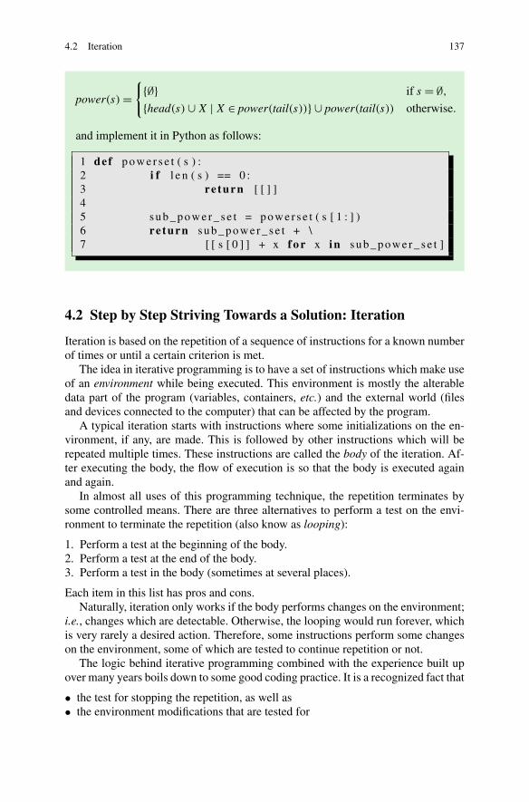
power(s) ={

{∅} if s = ∅,

{head(s) ∪ X | X ∈ power(tail(s))} ∪ power(tail(s)) otherwise.

and implement it in Python as follows:

1 def p o w e r s e t ( s ) :2 i f l e n ( s ) == 0 :3 re turn [ [ ] ]45 s u b _ p o w e r _ s e t = p o w e r s e t ( s [ 1 : ] )6 re turn s u b _ p o w e r _ s e t + \7 [ [ s [ 0 ] ] + x f o r x in s u b _ p o w e r _ s e t ]

4.2 Step by Step Striving Towards a Solution: Iteration

Iteration is based on the repetition of a sequence of instructions for a known numberof times or until a certain criterion is met.

The idea in iterative programming is to have a set of instructions which make useof an environment while being executed. This environment is mostly the alterabledata part of the program (variables, containers, etc.) and the external world (filesand devices connected to the computer) that can be affected by the program.

A typical iteration starts with instructions where some initializations on the en-vironment, if any, are made. This is followed by other instructions which will berepeated multiple times. These instructions are called the body of the iteration. Af-ter executing the body, the flow of execution is so that the body is executed againand again.

In almost all uses of this programming technique, the repetition terminates bysome controlled means. There are three alternatives to perform a test on the envi-ronment to terminate the repetition (also know as looping):

1. Perform a test at the beginning of the body.2. Perform a test at the end of the body.3. Perform a test in the body (sometimes at several places).

Each item in this list has pros and cons.Naturally, iteration only works if the body performs changes on the environment;

i.e., changes which are detectable. Otherwise, the looping would run forever, whichis very rarely a desired action. Therefore, some instructions perform some changeson the environment, some of which are tested to continue repetition or not.

The logic behind iterative programming combined with the experience built upover many years boils down to some good coding practice. It is a recognized fact that

• the test for stopping the repetition, as well as• the environment modifications that are tested for


Fig. 4.4 Pre-testing

Fig. 4.5 Post-testing

should be restricted to a single locality (not scattered over the iteration code). Ac-cordingly, four common patterns in the layout of the iterations have surfaced. A veryhigh percentage of iterations exhibit one of the patterns displayed in Figs. 4.4and 4.5.

In the Figures,

4.2 Iteration 139

• represents the whole environment that is used and/or modified in the itera-tion.

• represents the part of the environment that is modified and used in testing fortermination.

• represents all used and/or modified parts of the environment which are notused in testing for termination.

In addition to these four patterns, there is a fifth one, which is seldom used:A body where termination tests are performed at multiple points.

From the four patterns displayed, the least preferable one is the premod-posttesting (Fig. 4.5(a)) because it does not prevent undesired (due to some unantic-ipated ingredient) modifications from being used.

The conditional, as stated previously, has to be present in all programming lan-guages. Therefore, to implement these four iterative patterns, it is sufficient that thelanguage provides a branching instruction; imperative languages have branchinginstruction whereas pure functional languages do not. However, due to the over-whelming use of these patterns plus the anti-propaganda by the structured program-mers against the use of branching instructions, many imperative languages providea syntax for those patterns of iteration. The idea is to decouple the test and the body.Many languages provide a syntax that serve to implement pre-testing patterns andin addition, some provide a syntax for post-testing. The one for pre-testing is knownas the while construct and in many languages, it has the structure of:

while test do some_action(s)

The syntax for post-testing is known as the repeat. . . until construct and usually hasthe structure:

repeat some_action(s) until test

In this case, test is a termination condition (the looping continues until the testevaluates to TRUE). Sometimes, a variant of repeat exists where the test is forcontinuation (not for termination):

do some_action(s) while test

Some languages take it even further and provide syntax with dedicated slots for theinitialization, test, execution and modification (or some of them).

In the Python part of this section, you will find extensive examples and informa-tion about what Python supports in terms of those patterns and constructs.1

As we have mentioned earlier, the structured programming style denounces theexplicit use of branching instructions (gotos). For this reason, to fulfill the need ofending the looping (almost always based on a decision) while the body is being exe-cuted, some languages implement the break and continue constructs. A break

1Interestingly, you will observe that Python does not support the post-testing with a syntax, at all.


causes the termination of the body execution as well as the iteration itself and per-forms an immediate jump to the next action that follows the iteration. A continueskips over the rest of the actions to be executed and performs an immediate jump tothe test.2

Additional syntax exists for some combined needs for the modification and test-ing parts. Many iterative applications have needs that:

(a) Systematically explore all cases, or(b) Systematically consider some or all cases by jumping from one case to another

as a function of the previous case.

Below are some examples of these types of requirements:

• For each student in a class, compute the letter grade.[example to type (a)]

• Given a road map, for each city, display the neighboring cities.[example to type (b)]

• Given a road map, find the shortest path from a given city to another.[example to type (b)]

• For all the rows in a matrix, compute the mean.[example to type (a)]

• Find all the even numbers in the range [100000,250000].[example to type (a)]

• For all coordinates, compute the electromagnetic flux.[example to type (a)]

• Find the root of a given function using the Newton–Raphson method.[example to type (b)]

• Compute the total value of all the white pieces in a stage of a chess game.[example to type (a)]

• Compute all the possible positions to which a knight can move in three moves (ina chess game).[example to type (b)]

• For all the pixels in a digital image, compute the light intensity.[example to type (a)]

• Knowing the position of a white pixel, find the white area this pixel belongs to,which is bound by non-white boundary.[example to type (b)]

Especially regarding the (a) type of needs, many imperative languages provide theprogrammer with two kinds of iterators. In Computer Science, an iterator is a con-struct that allows a programmer to traverse through all the elements of

• a container, or• a range of numbers.

2Minor variations among languages can occur about the location to which the actual jump is made.

4.2 Iteration 141

The first kind of iterators, namely iteration over the members of a container, usuallyhave the following syntax:

foreach variable in container do some_action(s)

Certainly, keywords may vary from language to language.The second kind of iterators, namely iteration over a range of numbers, appear in

programming languages as:

for variable in start_value to end_value step increment dosome_action(s)

Here too, the keywords may vary. It is also possible that the order and even the syn-tax is different. However, despite all these minor syntactic variations, the semanticand the ingredients for this semantic remains common.

4.2.1 Tips for Creating Iterative Solutions

1. Work with a case example. Pay attention to the fact that the case should coverthe problem domain (i.e., the case is not a specific example of a subtype of theproblem).

2. Contrary to recursion, do not start by concentrating on the initial or terminal con-ditions. Start with a case example where the iteration has gone through severalcycles and partially built the solution.

3. If you take the pre-mod approach:Determine what is going to change and what is going to remain the same in thiscycle. Perform the changes that are doable.If you take the post-mod approach:Determine what must have been changed (from the previous cycle) and must notbe incorporated in the solution and what will remain the same in this cycle.

4. Having the half-completed solution to hand, determine the way you should mod-ify it to incorporate the ‘incremental’ changes that were performed in the periodprior to this point (those changes subject to (3) that were performed and have notyet been incorporated in the solution).

5. Determine the termination criteria. Make sure that the looping will terminate forall possible task cases.

6. For each variable whose value is used throughout the iteration, look for a propervalue being assigned to it, prior to the first use. The initialization part is ex-actly for this purpose. Those variables, used without having had a proper valueassigned, should be initialized here. The initialization values are, of course, task-dependent.

7. Consider the termination situation. If the task is going to produce a value, de-termine this value, secure it if necessary, and if the iteration is wrapped in afunction, then do not forget to properly return that value.

8. If you have to do some post processing (e.g. memory cleaning up, device discon-nection, etc.), consider them at this step. If you have written a function, do notforget that these actions must go before the return action.


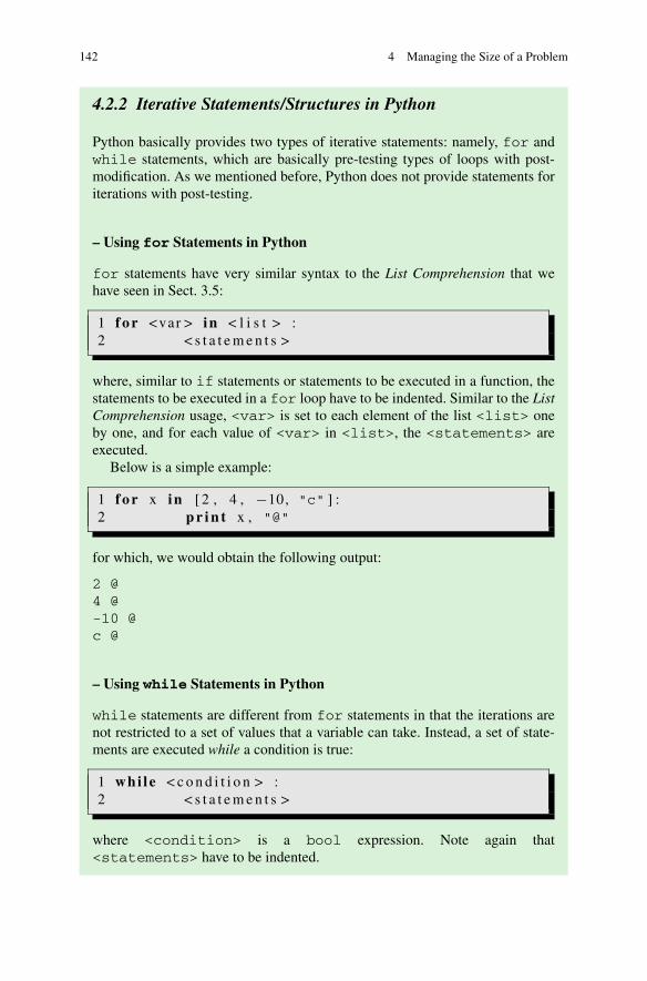
4.2.2 Iterative Statements/Structures in Python

Python basically provides two types of iterative statements: namely, for andwhile statements, which are basically pre-testing types of loops with post-modification. As we mentioned before, Python does not provide statements foriterations with post-testing.

– Using for Statements in Python

for statements have very similar syntax to the List Comprehension that wehave seen in Sect. 3.5:

1 f o r <var > in < l i s t > :2 < s t a t e m e n t s >

where, similar to if statements or statements to be executed in a function, thestatements to be executed in a for loop have to be indented. Similar to the ListComprehension usage, <var> is set to each element of the list <list> oneby one, and for each value of <var> in <list>, the <statements> areexecuted.

Below is a simple example:

1 f o r x in [ 2 , 4 , −10, "c" ] :2 p r i n t x , "@"

for which, we would obtain the following output:

2 @4 @-10 @c @

– Using while Statements in Python

while statements are different from for statements in that the iterations arenot restricted to a set of values that a variable can take. Instead, a set of state-ments are executed while a condition is true:

1 whi le < c o n d i t i o n > :2 < s t a t e m e n t s >

where <condition> is a bool expression. Note again that<statements> have to be indented.

4.2 Iteration 143

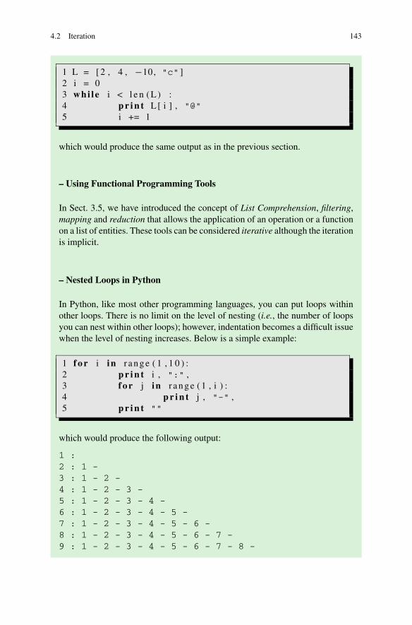
1 L = [ 2 , 4 , −10, "c" ]2 i = 03 whi le i < l e n ( L ) :4 p r i n t L [ i ] , "@"5 i += 1

which would produce the same output as in the previous section.

– Using Functional Programming Tools

In Sect. 3.5, we have introduced the concept of List Comprehension, filtering,mapping and reduction that allows the application of an operation or a functionon a list of entities. These tools can be considered iterative although the iterationis implicit.

– Nested Loops in Python

In Python, like most other programming languages, you can put loops withinother loops. There is no limit on the level of nesting (i.e., the number of loopsyou can nest within other loops); however, indentation becomes a difficult issuewhen the level of nesting increases. Below is a simple example:

1 f o r i in r a n g e ( 1 , 1 0 ) :2 p r i n t i , ":" ,3 f o r j in r a n g e ( 1 , i ) :4 p r i n t j , "-" ,5 p r i n t ""

which would produce the following output:

1 :2 : 1 -3 : 1 - 2 -4 : 1 - 2 - 3 -5 : 1 - 2 - 3 - 4 -6 : 1 - 2 - 3 - 4 - 5 -7 : 1 - 2 - 3 - 4 - 5 - 6 -8 : 1 - 2 - 3 - 4 - 5 - 6 - 7 -9 : 1 - 2 - 3 - 4 - 5 - 6 - 7 - 8 -


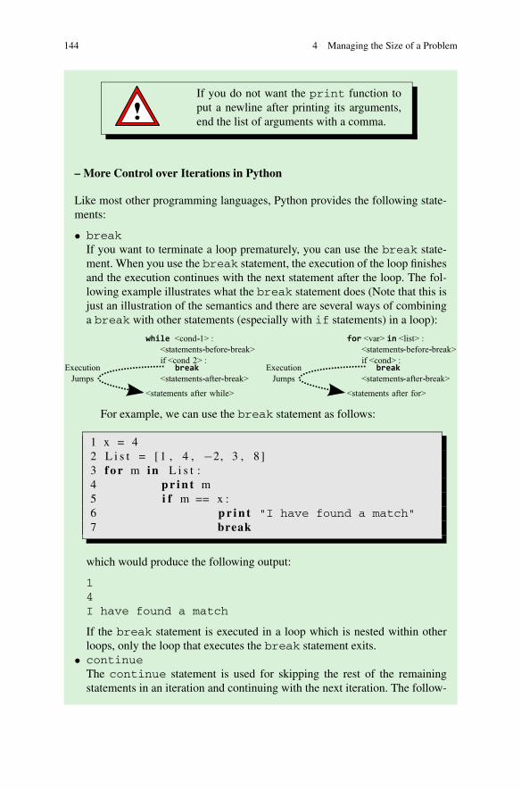
If you do not want the print function toput a newline after printing its arguments,end the list of arguments with a comma.

– More Control over Iterations in Python

Like most other programming languages, Python provides the following state-ments:

• breakIf you want to terminate a loop prematurely, you can use the break state-ment. When you use the break statement, the execution of the loop finishesand the execution continues with the next statement after the loop. The fol-lowing example illustrates what the break statement does (Note that this isjust an illustration of the semantics and there are several ways of combininga break with other statements (especially with if statements) in a loop):

For example, we can use the break statement as follows:

1 x = 42 L i s t = [ 1 , 4 , −2, 3 , 8 ]3 f o r m in L i s t :4 p r i n t m5 i f m == x :6 p r i n t "I have found a match"7 break


14I have found a match

If the break statement is executed in a loop which is nested within otherloops, only the loop that executes the break statement exits.

• continueThe continue statement is used for skipping the rest of the remainingstatements in an iteration and continuing with the next iteration. The follow-

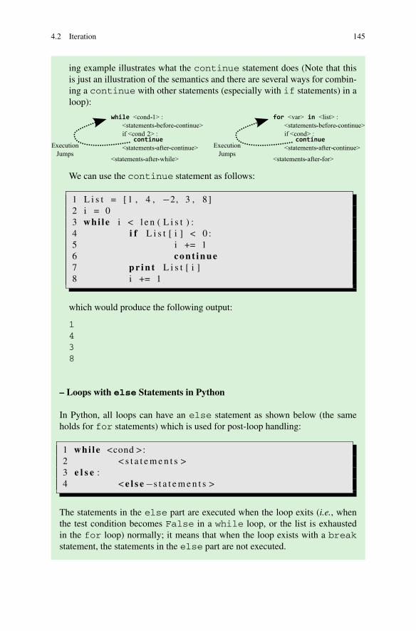
4.2 Iteration 145

ing example illustrates what the continue statement does (Note that thisis just an illustration of the semantics and there are several ways for combin-ing a continue with other statements (especially with if statements) in aloop):

We can use the continue statement as follows:

1 L i s t = [ 1 , 4 , −2, 3 , 8 ]2 i = 03 whi le i < l e n ( L i s t ) :4 i f L i s t [ i ] < 0 :5 i += 16 c o n t i n u e7 p r i n t L i s t [ i ]8 i += 1


1438

– Loops with else Statements in Python

In Python, all loops can have an else statement as shown below (the sameholds for for statements) which is used for post-loop handling:

1 whi le <cond >:2 < s t a t e m e n t s >3 e l s e :4 < e l s e −s t a t e m e n t s >

The statements in the else part are executed when the loop exits (i.e., whenthe test condition becomes False in a while loop, or the list is exhaustedin the for loop) normally; it means that when the loop exists with a breakstatement, the statements in the else part are not executed.


Fig. 4.6 Domain relations ofrecursive and iterativealgorithms

4.3 Recursion Versus Iteration

Numerous comparisons of these two techniques exist. A simple “recursion vs. it-eration” search on Google returns over 40,000 matches and the comparisons seemto be far from being coherent. The main reason is that the comparison is multidi-mensional and every individual has its own weighting on these dimensions. We willconsider each dimensi on individually.

4.3.1 Computational Equivalence

This can be expressed as a simple question

Disregarding the computational resources, does there exist a single problemwhich can be solved by one of the two techniques and not by the other?

The answer is a pure no. Furthermore, it can be proven that every iterative algorithmcan be converted into a recursive one and any recursive algorithm can be convertedinto an iterative one that makes use of stack data structure.

The need for a stack is sometimes unnecessary. In other words, the algorithmcan be re-engineered to get rid of the stack. For ‘tail recursion’, a certain type ofrecursion where the recursive call is the very last action in the definition, there exista proven transformation that removes the recursion. This transformation is called‘tail recursion removal’ and is sometimes automatically performed by compilers.Recursion removal is not confined to ‘tail recursion’. This is still a hot topic incomputer science and various scientists propose techniques to convert some of therecursive algorithms into iterative ones without using a stack.

Figure 4.6 depicts the equivalence relations of the two classes of algorithms andtheir subclasses.

4.3.2 Resource-Wise Efficiency

In contrary to the built-in facilities for arithmetical calculations and conditional con-trol of the execution flow, processors are not designed to natively support user de-

4.3 Recursion Versus Iteration 147

Table 4.1 Overhead costs for recursive and iterative calls

Function call Time overhead cost Memory overhead cost

Recursive n unit (k1 × n) bytes

Iterative (w/o stack) 1 unit k1 bytes

Iterative (with stack) 1 unit (k1 + k2 × n) bytes

k1,2 are constants and k1 > k2

fined function calls. High-level languages provide this facility by a series of pre-cisely implemented instructions and a stack-based short-term data structure (techni-cally named as activation records on acall stack). Therefore, when a function call ismade, the processor has lots of additional instructions to execute (in addition to theinstructions of the function), which means time. Furthermore, each call has somespatial cost in the memory, i.e., storage cost. Even for the ‘intelligently’ rewrittenrecursive Fibonacci(n) function, which fires only one recursion per call, this pro-cessing time and memory space overhead will grow in proportion to the value of n.On the other hand, a non-recursive definition of Fibonacci that does not need a stackwill not suffer from any n proportional call costs. Of course, one should not confusethis cost with the cost of the algorithmic computation: Both the recursive and thenon-recursive versions of Fibonacci consume additional time for adding n numbers,which is proportional to n.

We can summarize the resource cost for a function call with the sizable dimen-sion parameter as n in Table 4.1. What is the bottom line then?

• Resource wise the best is to have an algorithm which is iterative and is not needinga stack.

• Resource wise the second best is an iterative algorithm that requires a stack.• A Recursive algorithm is resource wise the worst.

4.3.3 From the Coder’s Viewpoint

• Since it is not an inherit technique of the human mind, ‘recursion’, at the firstsight, is easy to understand but not easy to construct. Therefore, the novice pro-grammer’s first reaction is to avoid recursion and stick to ‘iteration’. As the pro-grammer masters recursion, the shyness fades away and recursion gets frequentlypreferred over iteration. This is so because, for experienced programmers, recur-sive solutions are more apparent than imperative ones.

• Recursive solutions are more elegant, clean and easy to understand. They needfewer lines in coding compared to iterative ones. When clean code is more impor-tant than fast code, especially in the development phase, professionals will prefera recursive solution and consider it for iterative optimization at a later stage, ifnecessary.


• Recursive code is more likely to either function properly or do not function atall. Compared to recursive an iterative code is more cripple prone. That makesrecursive codes more difficult to trace and debug. On the other hand iterativecoding is more error prone which results in an increased need for tracing anddebugging.

4.4 Keywords

The important concepts that we would like our readers to understand in this chapterare indicated by the following keywords:

Bulkiness Recurrence RelationRecursion IterationLoop Tail Recursion

4.5 Further Reading

For more information on the topics discussed in this chapter, you can check out thesources below:

• Recursion:– http://en.wikipedia.org/wiki/Recursion– http://en.wikipedia.org/wiki/Recursion_%28computer_science%29

• Tail-recursion & its Removal:– http://en.wikipedia.org/wiki/Tail_recursion

• Iteration:– http://en.wikipedia.org/wiki/Iteration– http://en.wikipedia.org/wiki/While_loop– http://en.wikipedia.org/wiki/Do_while_loop– http://en.wikipedia.org/wiki/For_loop– http://en.wikipedia.org/wiki/Foreach

• Recursion to Iteration:– Y.A. Liu, S.D. Stoller, “From recursion to iteration: what are the optimiza-

tions?” Proceedings of the 2000 ACM SIGPLAN workshop on Partial evalua-tion and semantics-based program manipulation, 1999.

4.6 Exercises

1. What do you think the following Python code does? What happens when youcall the function like as follows: f(0)? How about f(-2)?

http://en.wikipedia.org/wiki/Recursion

http://en.wikipedia.org/wiki/Recursion_%28computer_science%29

http://en.wikipedia.org/wiki/Tail_recursion

http://en.wikipedia.org/wiki/Iteration

http://en.wikipedia.org/wiki/While_loop

http://en.wikipedia.org/wiki/Do_while_loop

http://en.wikipedia.org/wiki/For_loop

http://en.wikipedia.org/wiki/Foreach

4.6 Exercises 149

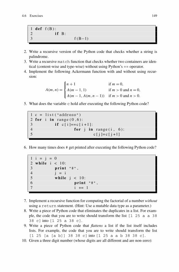
1 def f (B ) :2 i f B :3 f (B−1)

2. Write a recursive version of the Python code that checks whether a string ispalindrome.

3. Write a recursive match function that checks whether two containers are iden-tical (content-wise and type-wise) without using Python’s == operator.

4. Implement the following Ackermann function with and without using recur-sion:

A(m,n) =

⎧

⎪⎨

⎪⎩

n + 1 if m = 0,

A(m − 1,1) if m > 0 and n = 0,

A(m − 1,A(m,n − 1)) if m > 0 and n > 0.

5. What does the variable c hold after executing the following Python code?

1 c = l i s t ("address" )2 f o r i in r a n g e ( 0 , 6 ) :3 i f c [ i ]== c [ i + 1 ] :4 f o r j in r a n g e ( i , 6 ) :5 c [ j ]= c [ j +1]

6. How many times does # get printed after executing the following Python code?

1 i = j = 02 whi le i < 1 0 :3 p r i n t "#" ,4 j = i5 whi le j < 1 0 :6 p r i n t "#" ,7 i += 1

7. Implement a recursive function for computing the factorial of a number withoutusing a return statement. (Hint: Use a mutable data type as a parameter.)

8. Write a piece of Python code that eliminates the duplicates in a list. For exam-ple, the code that you are to write should transform the list [1 25 a a 3838 c] into [1 25 a 38 c].

9. Write a piece of Python code that flattens a list if the list itself includeslists. For example, the code that you are to write should transform the list[1 25 [a [a b]] 38 38 c] into [1 25 a a b 38 38 c].

10. Given a three digit number (whose digits are all different and are non-zero):


(a) We can derive two new three-digit numbers by sorting the three digits. Letus use A to denote the new number whose digits are in increasing order andB the number whose digits are in decreasing order. For example, for 392,A and B would respectively be 239 and 932.

(b) Subtracting A from B , we get a new number C (i.e., C = |B − A|).(c) If the result C has less than three digits, pad it from left with zeros; i.e., if

C is 63 for example, make it 063.(d) If C is not 1, continue from (a) with C as the three-digit number.It turns out that, for three-digit numbers, C eventually becomes 495 and neverchanges. This procedure outlined above is called the Kaprekar’s process andthe number 495 is known as the Kaprekar’s constant for three digits.Write a piece of Python code that finds the Kaprekar’s constant for four digitnumbers.

11. Write an iterative version of the recursive greatest-common-divisor functionthat we have provided in the chapter. Which version is easier for you to writeand understand?

12. Write an iterative version of the recursive power-set function that we have pro-vided in the chapter. Which version is easier for you to write and understand?

13. Some integers, called self numbers, have the property that they can be generatedby taking smaller integers and adding their digits together. For example, 21 canbe generated by summing up 15 with the digits of 15; i.e., 21 = 15 + 1 + 5. Onthe other hand, 20 is a self number since it cannot be generated from a smallerinteger (i.e., for any two digit number ab < 20, the equation 20 = ab + a + b

does not hold; or, more formally, ∀ab (ab < 20) ⇒ (20 �= ab + a + b)). Writea piece of Python code for finding self numbers between 0 and 1000.

14. Write a piece of Python code to check whether the following function convergesto a constant n value (Hint: It does).

f (n) ={

f (n/2) if nmod 2 = 0,

f (3n + 1) if nmod 2 = 1.

introduction to programming concepts with case studies in python || managing the size of a problem

Documents