introduction to programming in...
TRANSCRIPT

Introduction to Programming in ATS
Hongwei Xi
hwxi AT cs DOT bu DOT edu

Introduction to Programming in ATS:by Hongwei Xi
Copyright © 2010-201? Hongwei Xi
All rights are reserved. Permission is granted to print this document for personal use.

Dedication
To Jinning and Zoe.

4
Table of ContentsPreface ................................................................................................................................... ixI. Basic Functional Programming.......................................................................................1
1. Preparation for Starting...........................................................................................1A Running Program ...........................................................................................1A Template for Single-File Programs...............................................................1A Makefile Template ..........................................................................................2
2. Elements of Programming ......................................................................................5Expressions and Values......................................................................................5Names and Bindings ..........................................................................................5Scopes for Bindings ............................................................................................6Environments for Evaluation............................................................................7Static Semantics...................................................................................................7Primitive Types ...................................................................................................7Tuples and Tuple Types .....................................................................................8Records and Record Types ................................................................................9Conditional Expressions..................................................................................10Sequence Expressions ......................................................................................11Comments in Code...........................................................................................11
3. Functions .................................................................................................................13Functions as a Simple Form of Abstraction ..................................................13Function Arity ...................................................................................................14Function Interface.............................................................................................14Evaluation of Function Calls...........................................................................15Recursive Functions .........................................................................................15Evaluation of Recursive Function Calls ........................................................16Example: Coin Changes...................................................................................17Tail-Call and Tail-Recursion............................................................................18Example: Solving the Eight Queens Puzzle..................................................18Mutually Recursive Functions........................................................................21Mutual Tail-Recursion......................................................................................22Envless Functions and Closure Functions ....................................................23Higher-Order Functions ..................................................................................24Example: Binary Search ...................................................................................25Currying and Uncurrying ...............................................................................25
4. Datatypes.................................................................................................................27Patterns...............................................................................................................27Pattern-Matching ..............................................................................................27Matching Clauses and Case-Expressions......................................................28Enumerative Datatypes ...................................................................................28Recursive Datatypes.........................................................................................29Exhaustiveness of Pattern-Matching .............................................................30Example: Evaluating Integer Expressions.....................................................31
5. Parametric Polymorphism ....................................................................................35Function Templates ..........................................................................................35Polymorphic Functions....................................................................................36Polymorphic Datatypes ...................................................................................37Example: Function Templates on Lists ..........................................................38Example: Mergesort on Lists...........................................................................40
6. Summary .................................................................................................................43II. Support for Practical Programming ...........................................................................45
7. Effectful Programming Features ..........................................................................45Exceptions..........................................................................................................45Example: Testing for Braun Trees...................................................................47References ..........................................................................................................48Example: Implementing Counters .................................................................49Arrays.................................................................................................................50Example: Ordering Permutations ..................................................................51
v

Matrices..............................................................................................................53Example: Estimating the Constant Pi ............................................................54Simple Input and Output ................................................................................55
8. Convenience in Programming..............................................................................59Macro Definitions .............................................................................................59Compile-Time Directives .................................................................................61Overloading.......................................................................................................61
9. Modularity ..............................................................................................................63Types as a Form of Specification.....................................................................63Static and Dynamic ATS Files .........................................................................64Generic Template Implementation.................................................................66Abstract Types...................................................................................................66Example: A Package for Rationals .................................................................68Example: A Functorial Package for Rationals ..............................................69Specific Template Implementation.................................................................71Example: A Temptorial Package for Rationals .............................................72
10. Library Support ....................................................................................................75The prelude Library .........................................................................................75The libc Library.................................................................................................75The libats Library..............................................................................................75Contributed Packages ......................................................................................75
11. Interaction with the C Programming Language..............................................7712. Summary ...............................................................................................................79
III. Dependent Types for Programming.........................................................................8113. Introduction to Dependent Types ......................................................................81
Enhanced Expressiveness for Specification ..................................................81Constraint-Solving during Typechecking .....................................................84Example: String Processing .............................................................................85Example: Binary Search on Arrays.................................................................86Termination-Checking for Recursive Functions ..........................................87Example: Dependent Types for Debugging..................................................89
14. Datatype Refinement ...........................................................................................91Dependent Datatypes.......................................................................................91Example: Function Templates on Lists (Redux)...........................................93Example: Mergesort on Lists (Redux) ...........................................................95Sequentiality of Pattern Matching..................................................................96Example: Functional Random-Access Lists ..................................................97Example: Functional Red-Black Trees..........................................................101
15. Theorem-Proving in ATS/LF ...........................................................................105Encoding Relations as Dataprops ................................................................105Constructing Proofs as Total Functions.......................................................106Example: Proving Distributivity of Multiplication....................................107Datasorts ..........................................................................................................108Example: Proving Properties on Braun Trees .............................................110
16. Programming with Theorem-Proving.............................................................115Circumventing Nonlinear Constraints ........................................................115Example: Safe Matrix Subscripting ..............................................................116Specifying with Enhanced Precision............................................................117Example: Another Verified Factorial Implementation ..............................118Example: Verified Fast Exponentiation .......................................................119
17. Summary .............................................................................................................123IV. Linear Types for Programming................................................................................125
18. Introduction to Views and Viewtypes.............................................................125Views for Memory Access through Pointers ..............................................125Viewtypes as a Combination of Views and Types .....................................127Left-Values and Call-by-Reference...............................................................128Stack-Allocated Variables ..............................................................................129
19. Dataviews as Linear Dataprops .......................................................................131Optional Views................................................................................................131
vi

Linear Arrays ..................................................................................................132Singly-Linked Lists.........................................................................................134Proof Functions for View Changes...............................................................137Example: Quicksort ........................................................................................140
20. Dataviewtypes as Linear Datatypes ................................................................145Linear Optional Values ..................................................................................145Linear Lists ......................................................................................................146Example: Mergesort on Linear Lists ............................................................149Linear Binary Search Trees ............................................................................152Transition from Datatypes to Dataviewtypes.............................................155
21. Abstract Views and Viewtypes.........................................................................161Memory Allocation and Deallocation .........................................................161Simple Linear Objects ....................................................................................162Example: Implementing an Array-Based Circular Buffer ........................165From linearity to non-linearity .....................................................................166
22. Summary .............................................................................................................169
vii

viii
Preface
ATS1 is a statically typed programming language that unifies implementation withformal specification. Within ATS, there are two sublanguages: one for specificationand the other for implementation, and there is also a theorem-proving subsystem forverifying whether an implementation indeed implements according to its specifica-tion. If I could associate only one single word with ATS, I would choose the wordprecision. Programming in ATS is about being precise and being able to effectivelyenforce precision. This point will be demonstrated concretely and repeatedly in thisbook.
In order to be precise in building software systems, we need to specify what sucha system is expected to accomplish. In the current day and age, software specifica-tion, which we use in a rather loose sense, is often done in forms of varying degreeof formalism, ranging from verbal discussions to pencil/paper drawings to variousdiagrams in modeling languages such as UML to formal specifications in specifi-cation languages such as Z2, etc. Often the main purpose of software specificationis to establish some mutual understanding among a team of developers. After thespecification for a software system is done, either formally or informally, we needto implement the specification in a programming language. In general, it is exceed-ingly difficult to be reasonably certain whether an implementation actually meets itsspecification. Even if the implementation coheres well with its specification initially,it nearly inevitably diverges from the specification as the software system evolves.The dreadful consequences of such a divergence are all too familiar; the specificationbecomes less and less reliable for understanding the behavior of the software systemwhile the implementation gradually turns into its own specification; for the develop-ers, it becomes increasingly difficult and risky to maintain and extend the softwaresystem; for the users, it requires increased amount of time and effort to learn and usethe software system.
Largely inspired by Martin-Loef’s constructive type theory, which was originally de-veloped for the purpose of establishing a foundation for mathematics, I designedATS in an attempt to combine specification and implementation into a single pro-gramming language. There are a static component (statics) and a dynamic component(dynamics) in ATS. Intuitively, the statics and dynamics are each for handling typesand programs, respectively. In particular, specification is done in the statics. Given aspecification, how can we then effectively ensure that an implementation of the spec-ification (type) indeed implements according to the specification? We request thatthe programmer who does the implementation also construct a proof in the theorem-proving subsystem of ATS to demonstrate it. This is a style of program verificationthat puts the programmer at the center, and thus we refer to it as a programmer-centric approach to program verification.
ATS is also a feature-rich programming language. It can support a variety of pro-gramming paradigms, including functional programming, imperative programming,object-oriented programming, concurrent programming, modular programming, etc.However, the core of ATS, which is based on a call-by-value functional language, issurprisingly simple, and this is where the journey of programming in ATS starts.In this book, I will demonstrate primarily through examples how various program-ming features in ATS can be employed effectively to facilitate the construction ofhigh-quality programs. I will focus on programming practice instead of program-ming theory. If you are primarily interested in the type-theoretical foundation of ATS,then you have to find it elsewhere.
If you can implement, then you are a good programmer. In order to be a better pro-grammer, you should also be able to explain what you implement. If you can guar-antee what is implemented matches what is specified, then you are surely the bestprogrammer. Hopefully, learning ATS will put you on a wonderful exploring jour-ney to become the best programmer. Let that journey start now!
ix
Preface
Notes1. http://www.ats-lang.org
2. http://www.afm.sbu.ac.uk/zbook
x

Chapter 1. Preparation for Starting
It is most likely that you want to write programs in the programming language youare learning. You may also want to try some of the examples included in this bookand see what really happens. So I will first show you how to write in ATS a single-fileprogram, that is, a program contained in a single file, and compile it and then executeit.
A Running ProgramThe following example is a program in ATS that prints out (onto the console) thestring "Hello, world!" and a newline before it terminates:
val _void_ = print ("Hello, world!")implement main () = () // a dummy implementation for [main]
The keyword val initiates a binding between the variable _void_ and the function callprint ("Hello, world! "). However, this binding is never used after it is introduced; itssole purpose is for the call to the print function to get evaluated.
The function main is of certain special meaning in ATS, which I will explain else-where. For a programmer who knows the C or Java programming language, I simplypoint out that the role of main is essentially the same as its counterpart of the samename in C or Java. The keyword implement initiates the implementation of a func-tion whose interface has already been declared elsewhere. The declared interface formain in ATS is given as follows:
fun main (): void
which indicates that main is a nullary function, that is, a function that takes no argu-ments, and it returns no value (or it returns the void value). The double slash symbol(//) initiates a comment that terminates at the end of the current line.
Suppose that you have already installed the ATS programming language system. Youcan issue the following command-line to generate an executable named hello in thecurrent working directory:
atscc -o hello hello.dats
where hello.dats is a file containing the above program. Note that the filenameextension .dats should not be altered as it has already been assigned a special meaningthat the compilation command atscc recognizes. Another special filename extensionis .sats, which we will encounter elsewhere.
A Template for Single-File ProgramsThe following code template, which is available on-line1, is designed for constructinga single-file program in ATS:
(***** This is a template for a single-file ATS program***)
(* ****** ****** *)
1

Chapter 1. Preparation for Starting
(*** please do not change unless you know what you do*)//staload _(*anon*) = "libc/SATS/stdio.sats"//staload _(*anon*) = "prelude/DATS/array.dats"staload _(*anon*) = "prelude/DATS/array0.dats"//staload _(*anon*) = "prelude/DATS/list.dats"staload _(*anon*) = "prelude/DATS/list0.dats"staload _(*anon*) = "prelude/DATS/list_vt.dats"//staload _(*anon*) = "prelude/DATS/matrix.dats"staload _(*anon*) = "prelude/DATS/matrix0.dats"//staload _(*anon*) = "prelude/DATS/option.dats"staload _(*anon*) = "prelude/DATS/option0.dats"//staload _(*anon*) = "prelude/DATS/pointer.dats"//staload _(*anon*) = "prelude/DATS/reference.dats"//(* ****** ****** *)
//// please write you program in this section//
(* ****** ****** *)
implement main () = () // a dummy implementation for [main]
Each line starting with the keyword staload essentially allows the ATS compiler at-sopt to gain access to the definition of certain library functions. I will cover elsewherein the book the topic on programming with library functions in ATS.
A Makefile TemplateThe following Makefile template, which is available on-line2, is provided to help youconstruct your own Makefile for compiling ATS programs. If you are not familiarwith the make utility, you could readily find plenty resources on-line to help yourselflearn it.
###### A Makefile template for compiling ATS programs####
######
ATSUSRQ="$(ATSHOME)"ifeq ($(ATSUSRQ),"")ATSUSRQ="/usr"endif # end of [ifeq]
######
ATSCC=$(ATSUSRQ)/bin/atsccATSOPT=$(ATSUSRQ)/bin/atsopt
######
2

Chapter 1. Preparation for Starting
## Please uncomment the one you want, or skip it entirely#ATSCCFLAGS=#ATSCCFLAGS=-O2## [-flto] enables link-time optimization such as inlining lib functions##ATSCCFLAGS=-O2 -flto
######
## HX: Please uncomment it if you need to run GC at run-time#ATSGCFLAG=#ATSGCFLAG=-D_ATS_GCATS
######
distclean::
######
## Please uncomment the following three lines and replace the name [foo]# with the name of the file you want to compile#
# foo: foo.dats# $(ATSCC) $(ATSGCFLAG) $(ATSCCFLAGS) -o $@ $< || touch $@# distclean:: ; $(RMF) foo
######
## You may find these rules useful#
# %_sats.o: %.sats# $(ATSCC) $(ATSCCFLAGS) -c $< || touch $@
# %_dats.o: %.dats# $(ATSCC) $(ATSCCFLAGS) -c $< || touch $@
######
RMF=rm -f
######
clean:$(RMF) *~$(RMF) *_?ats.o$(RMF) *_?ats.c
distclean:: clean
###### end of [Makefile] ######
3

Chapter 1. Preparation for Starting
Notes1. http://www.ats-lang.org/DOCUMENT/INTPROGINATS/CODE/CHAPTER_START/mytest.dats
2. http://www.ats-lang.org/DOCUMENT/INTPROGINATS/CODE/CHAPTER_START/Makefile_template
4
Chapter 2. Elements of Programming
The core of ATS is a call-by-value functional programming language. I will explainthe meaning of call-by-value in a moment. As for functional programming, there isreally no precise definition. The most important aspect of functional programmingthat I want to explore is the notion of binding, which relates names to expressions.
Expressions and ValuesATS is feature-rich, and its grammar is probably more complex than most existingprogramming languages. In ATS, there are a large variety of forms of expressions,which I will introduce gradually.
Let us first start with some integer arithmetic expressions (IAEs): 1, ~2, 1+2, 1+2*3-4,(1+2)/(3-4), etc. Note that the negative sign is represented by the tilde symbol (~)in ATS. There is also support for floating point numbers, and some floating pointconstants are given here: 1.0, ~2.0, 3., 0.12345, 2.71828, 31416E-4, etc. Note that 3. and31416E-4 are the same as 3.0 and 3.1416, respectively. What I really want to emphasizeat this point is that 1 and 1.0 are two distinct numbers in ATS: the former is an integerwhile the latter is a floating point number.
There are also boolean constants: true and false. We can form boolean expressionssuch as 1 >= 0, not(2-1 >= 2), (1 < 2) andalso (2 < 3) and (~1 > 1) orelse (~1 <= 1), wherenot, andalso and orelse stand for negation, conjunction and disjunction, respectively.
Other commonly used constant values include characters and strings. For instance,here are some character constants: ’a’, ’B’, ’ ’ (newline), ’ ’ (tab), ’(’ (left parenthesis),’)’ (right parenthesis), ’{’ (left curly brace), ’}’ (right curly brace), etc; here are somestring constants: "My name is Zoe", "Don’t call me "Cloe"", "this is a newline: ", etc.
Given a (function) name, say, foo, and an expression exp, the expression foo(exp) is afunction application or function call. The parentheses in foo(exp) may be dropped ifno ambiguity is created by doing so. For instance, print("Hello") is a function appli-cation, which can also be written as print "Hello". If foo is a nullary function, then afunction application foo() can be formed. If foo is a binary function, then a functionapplication foo(exp1, exp2) can be formed for expressions exp1 and exp2. Functionsof more arguments can be treated accordingly.
Note that we cannot write +(1,2) as the name + has already been given the infix sta-tus requiring that it be treated as an infix operator. However, we can write op+(1,2),where op is a keyword in ATS that can be used to temporarily suspend the infix sta-tus of any name immediately following it. I will explain in detail the issue of fixity(prefix, infix and postfix) elsewhere.
Values are essentially expressions of certain special forms, which can not be reducedor simplified further. For instance, integer constants such as 1 and ~2 are values,but the integer expression 1+2 is not a value, which can be reduced to the value 3.Evaluation refers to the computational process that reduces a given expression intoa value. However, certain expressions such as 1/0 cannot be reduced to a value, andevaluating such an expression must abort at some point. I will gradually presentmore information on evaluation.
Names and BindingsA crucial aspect of a programming language is the mechanism it provides for bindingnames, which are themselves expressions, to expressions. For instance, a declarationis introduced by the following syntax that declares a binding between the name x,which is also referred to as a variable, and the expression 1+2:
val x = 1 + 2
5

Chapter 2. Elements of Programming
Note that val is a keyword in ATS, and the declaration is classified as aval-declaration. Conceptually, what happens at run-time in a call-by-value languagesuch as ATS is that the expression 1+2 is first evaluated to the value 3, and then thebinding between x and 1+2 is finalized into a binding between x and 3. Essentially,call-by-value means that a binding between a name and an expression needs to befinalized into one between the name and the value of the expression before it can beused in evaluation subsequently. As another example, the following syntax declaresthree bindings, two of which are formed simultaneously in the first line:
val PI = 3.14 and radius = 10.0val area = PI * radius * radius
Note that it is unspecified in ATS as to which of the first two bindings is finalizedahead of the other at run-time. However, it is guaranteed that the third binding isfinalized after the first two are done.
Scopes for BindingsEach binding is given a fixed scope in which the binding is considered legal or effec-tive. The scope of a toplevel binding in a file starts from the point where the bindingis introduced until the very end of the file. The bindings introduced in the follow-ing example between the keywords let and in are effective until the keyword end isreached:
val area = letval PI = 3.14 and radius = 10.0 in PI * radius * radius
end // end of [let]
Such bindings are referred to as local bindings, and the names such as PI and radiusare referred to as local names. This example can also be written in the following style:
val area =PI * radius * radius where {val PI = 3.14 and radius = 10.0 // simultaneous bindings
} // end of [where]
The keyword where appearing immediately after an expression introduces bindingsthat are solely effective for evaluating names contained in the expression. Note thatexpressions formed using the keywords let and where are often referred to as let-expressions and where-expressions, respectively. The former can always be trans-lated into the latter directly and vice versa. Which style is better? I have not formedmy opinion yet. The answer seems to entirely depend on the taste of the programmer.
The following example demonstrates an alternative approach to introducing localbindings:
local
val PI = 3.14 and radius = 10.0
in
val area = PI * radius * radius
end // end of [local]
where the bindings introduced between the keywords local and in are effective untilthe keyword end is reached. Note that the bindings introduced between the key-words in and end are themselves toplevel bindings. The difference between let and
6

Chapter 2. Elements of Programming
local should be clear: The former is used to form an expression while the latter is usedto introduce a sequence of declarations.
Environments for EvaluationEvaluation is the computational process that reduces expressions to values. Whenperforming evaluation, we need not only the expression to be evaluated but also acollection of bindings that map names in the expression to values. This collection ofbindings, which is just a finite mapping, is often referred to as an environment (forevaluation). For instance, suppose that we want to evaluate the following expression:
letval PI = 3.14 and radius2 = 10.0 * 10.0 in PI * radius2
end
We start with the empty environment ENV0; we evaluate 3.14 to itself and 10.0 *10.0 to 100.0 under the environment ENV0; we then extend ENV0 to ENV1 with twobindings mapping PI to 3.14 and radius2 to 100.0; we then evaluate PI * radius2 underENV1 to 3.14 * radius2, then to 3.14 * 100.0, and finally to 314.0, which is the value ofthe let-expression.
Static SemanticsATS is a programming language equipped with a highly expressive type systemrooted in the Applied Type System framework, which also gives ATS its name. I willgradually introduce the type system of ATS, which is probably the most outstandingand interesting part of this book.
It is common to treat a type as the set of values it classifies. However, I find it moreapproriate to treat a type as a form of meaning. There are formal rules for assign-ing types to expressions, which are referred to as typing rules. If a type T can beassigned to an expression, then I say that the expression possesses the static meaning(semantics) represented by the type T. Note that an expression may be assigned manydistinct static meanings. An expression is well-typed if there exists a type T such thatthe expression can be assigned the type T.
If there is a binding between a name and an expression and the expression is of sometype T, then the name is assumed to be of the type T in the effective scope of thebinding. In other words, the name assumes the static meaning of the expression itrefers to.
Let exp0 be an expression of some type T, that is, the type T can be assigned to exp0according to the typing rules. If we can evaluate exp0 to exp1, then exp1 can also beassigned the type T. In other words, static meaning is an invariant under evaluation.This property is often referred to as type preservation, which is part of the soundnessof the type system of ATS. Based on this property, we can readily infer that any valueis of the type T if exp0 can be evaluated to it (in many steps).
Let exp0 be an expression of some type T. Assume that exp0 is not a value. Then exp0can always be evaluated one step further to another expression exp1. This propertyis often referred to as progress, which is another part of the soundness of the typesystem of ATS.
7
Chapter 2. Elements of Programming
Primitive TypesThe simplest types in ATS are primitive types, which are used to classify primitivevalues. For instance, we have the primitive types int and double, which classify inte-gers (in a fixed range) and floating point numbers (of double precision), respectively.
In the current implementation of ATS (Anairiats), a program in ATS is first compiledinto one in C, which can then be compiled to object code by a compiler for C such asgcc. In the compilation from ATS to C, the type int in ATS is translated to the type ofthe same name in C. Similarly, the type double in ATS is translated to the type of thesame name in C.
There are many other primitive types in ATS, and I will introduce them gradually.Some commonly used primitive types are listed as follows:
• bool: This type is for boolean values true and false.
• char: This type is translated into the type in C for characters.
• schar: This type is translated into the type in C for signed characters.
• uchar: This type is translated into the type in C for unsigned characters.
• float: This type is translated into the type in C for floating point numbers of singleprecision.
• uint: This type is translated into the type in C for unsigned integers.
• lint: This type is translated into the type in C for long integers.
• ulint: This type is translated into the type in C for unsigned long integers.
• llint: This type is translated into the type in C for long long integers.
• ullint: This type is translated into the type in C for unsigned long long integers.
• size_t: This type is translated into the type in C of the same name, which is forunsigned integers of certain precision.
• string: This type is for strings, and its translation in C is the type void* (for point-ers). I will explain this translation elsewhere.
• void: This type is for the void value, and its translation in C is the type void (forpointers). It should be noted that the void value is unspecified in ATS. I often saythat a function returns no value if it returns the void value, and vice versa.
I will gradually present programming examples involving various primitive typesand values.
Tuples and Tuple TypesGiven two types T1 and T2, we can form a tuple type (T1, T2), which can also bewritten as @(T1, T2). Assume that exp1 and exp2 are two expressions of the types T1and T2, respectively. Then the expression (exp1, exp2), which can also be written as@(exp1, exp2), refers to a tuple of the tuple type (T1, T2). Accordingly, we can formtuples and tuple types of more components. In order for a tuple type to be assignedto a tuple, the tuple and tuple type must have the equal number of components.
When evaluating a tuple expression, we evaluate all of its components sequentially.Suppose that the expression contains n components, then the value of the expressionis the tuple consisting of the n values of the n components listed in the order as thecomponents themselves.
A tuple of length n for n >= 2 is just a record of field names ranging from 0 untiln-1, inclusively. Given an expression exp of some tuple type (T1, T2), we can formexpressions (exp).0 and (exp).1, which are of types T1 and T2, respectively. Note thatthe expression exp does not have to be a tuple expression. For instance, exp may bea name or a function application. If exp evaluates to a tuple of two values, then exp.0
8

Chapter 2. Elements of Programming
evaluates to the first value and exp.1 the second value. Clearly, if the tuple type ofexp contains more components, what is stated can be generalized accordingly.
In the following example, we first construct a tuple of length 3 and then introducebindings between 3 names and all of the 3 components of the tuple:
val xyz = (’A’, 1, 2.0)val x = xyz.0 and y = xyz.1 and z = xyz.2
Note that the constructed tuple can be assigned the tuple type (char, int, double). An-other method for selecting components in a given tuple is based on pattern matching,which is employed in the following example:
val xyz = (’A’, 1, 2.0)val (x, y, z) = xyz // x = ’A’; y = 1; z = 2.0
Note that (x, y, z) is a pattern that can match any tuples of exact 3 components. I willsay more about pattern matching elsewhere.
The tuples introduced above are often referred to as flat tuples, native tuples or un-boxed tuples. There is another kind of tuples supported in ATS, which are calledboxed tuples. A boxed tuple is essentially a pointer pointing to some heap locationwhere a flat tuple is stored.
Assume that exp1 and exp2 are two expressions of the types T1 and T2, respectively.Then the expression ’(exp1, exp2), refers to a tuple of the tuple type ’(T1, T2). Ac-cordingly, we can form boxed tuples and boxed tuple types of fewer or more compo-nents. What should be noted immediately is that every boxed tuple is of the size of apointer, and can thus be stored in any place where a pointer can. Using boxed tuplesis rather similar to using unboxed ones. For instance, the meaning of the followingcode should be evident:
val xyz = ’( ’A’, 1, 2.0 )val x = xyz.0 and y = xyz.1 and z = xyz.2
Note that a space is needed between ’( and ’A’ for otherwise the current parser (forAnairiats) would be confused.
Given the availability of flat and boxed tuples, one naturally wants to know whetherthere is a simple way to determine which kind is preferred over the other. Unfortu-nately, there is no simple way to do this as far as I can tell. In order to be certain, somekind of profiling is often needed. However, if we want to run code with no supportof garbage collection (GC), then we should definitely avoid using boxed tuples.
Records and Record TypesA record is just like a tuple except that each field name of the record is chosen by theprogrammer (instead of being fixed). Similarly, a record type is just like a tuple type.For instance, a record type point2D is defined as follows:
typedef point2D = @{ x= double, y= double }
where x and y are the names of the two fields in a record value of this type. Wealso refer to a field in a record as a component. The special symbol @{ indicates thatthe formed type is for flat/native/unboxed records. A value of the type point2D isconstructed as follows and given the name theOrigin:
val theOrigin = @{ x= 0.0, y= 0.0 } : point2D
9

Chapter 2. Elements of Programming
We can use the standard dot notation to extract out a selected component in a record,and this is shown in the next line of code:
val theOrigin_x = theOrigin.x and theOrigin_y = theOrigin.y
Alternatively, we can use pattern matching for doing component extraction as is donein the next line of code:
val @{ x= theOrigin_x, y= theOrigin_y } = theOrigin
In this case, the names theOrigin_x and theOrigin_y are bound to the componentsin theOrgin that are named x and y, respectively. If we only need to extract out aselected few of components (instead of all the available ones), we can make use ofthe following kind of patterns:
val @{ x= theOrigin_x, ... } = theOrigin // the x-component onlyval @{ y= theOrigin_y, ... } = theOrigin // the y-component only
If you find all this syntax for component extraction to be confusing, then I suggestthat you stick to the dot notation. I myself rarely use pattern matching on recordvalues.
Compared with handling native/flat/unboxed records, the only change needed forhandling boxed records is to replace the special symbol @{ with another one: ’{, whichis a quote followed immediately by a left curly brace.
Conditional ExpressionsA conditional expression consists of a test and two branches. For instance, the fol-lowing expression is conditional:
if (x >= 0) then x else ~x
where if, then and else are keywords in ATS. In a conditional expression, the expres-sion following if is the test and the expressions following then and else are referred toas the then-branch and the else-branch (of the conditional expression), respectively.
In order to assign a type T to a conditional expression, we need to assign the typebool to the test and the type T to both of the then-branch and the else-branch. Forinstance, the type int can be assigned to the above conditional expression if the namex is given the type int. One may think that the following conditional expression isill-typed, that is, it cannot be given type:
if (x >= 0) then ’0’ else 1 // this expression can be given a type!
Actually, it is possible to find a type T in ATS that can be assigned to the conditionalexpression. I will explain the reason for this elsewhere.
Suppose that we have a conditional expression that is well-typed. When evaluating it,we first evaluate the test to a value, which is guaranteed to be either true or false; if thevalue is true, then we continue to evaluate the then-branch; otherwise, we continueto evaluate the else-branch.
It is also allowed to form a conditional expression where the else-branch is truncated.For instance, we can form something as follows:
if (x >= 0) then print(x)
10

Chapter 2. Elements of Programming
which is equivalent to the following conditional expression:
if (x >= 0) then print(x) else ()
Note that () stands for the void value (of the type void). If a type can be assigned to aconditional expression in the truncated form, then the type must be void.
Sequence ExpressionsAssume that exp1 and exp2 are expressions of types T1 and T2 respectively, whereT1 is void. Then a sequence expression (exp1; exp2) can be formed that is of the typeT2. When evaluating the sequence expression (exp1; exp2), we first evaluate exp1 tothe void value and then evaluate exp2 to some value, which is also the value of thesequence expression. When more expressions are sequenced, all of them but the lastone need to be of the type void and the type of the last expression is also the typeof the sequence expression being formed. Evaluating a sequence of more expressionsis analogous to evaluating a sequence of two. The following example is a sequenceexpression:
(print ’H’; print ’e’; print ’l’; print ’l’; print ’o’)
Evaluating this sequence expression prints out (onto the console) the 5-letter string"Hello". Instead of parentheses, we can also use the keywords begin and end to forma sequence expression:
beginprint ’H’; print ’e’; print ’l’; print ’l’; print ’o’
end // end of [begin]
If we like, we may also add a semicolon immediately after the last expression in asequence as long as the last expression is of the type void. For instance, the aboveexample can also be written as follows:
beginprint ’H’; print ’e’; print ’l’; print ’l’; print ’o’;
end // end of [begin]
I also want to point out the following style of sequencing:
letval () = print ’H’val () = print ’e’val () = print ’l’val () = print ’l’val () = print ’o’
in// nothing
end // end of [begin]
which is rather common in functional programming.
11

Chapter 2. Elements of Programming
Comments in CodeATS currently supports four forms of comments: line comment, block comment ofML-style, block comment of C-style, and rest-of-file comment.
• A line comment starts with the double slash symbol (//) and extends until the endof the current line.
• A block comment of ML-style starts and closes with the tokens (* and *), respec-tively. Note that nested block comments of ML-style are allowed, that is, one blockcomment of ML-style can occur within another one of the same style.
• A block comment of C-style starts and closes with the tokens /* and */, respec-tively. Note that block comments of C-style cannot be nested. The use of blockcomments of C-style is primarily in code that is supposed to be shared by ATS andC. In other cases, block comments of ML-style should be the preferred choice.
• A rest-of-file comment starts with the quadruple slash symbol (////) and extendsuntil the end of the file. Comments of this style of are particularly useful for thepurpose of debugging.
12

Chapter 3. Functions
Functions play a foundational role in programming. While it may be theoreticallypossible to program without functions (but with loops), such a programming style isof little practical value. ATS does provide some language constructs for implement-ing for-loops and while-loops directly. I, however, strongly recommend that the pro-grammer implement loops as recursive functions or more precisely, as tail-recursivefunctions. This is a programming style that matches well with more advanced pro-gramming features in ATS that will be presented in this book later.
The code employed for illustration in this chapter plus some additional code for test-ing is available on-line1.
Functions as a Simple Form of AbstractionGiven an expression exp of the type double, we can multiply exp by itself to computeits square. If exp is a complex expression, we may introduce a binding between aname and exp so that exp is only evaluated once. This idea is shown in the followingexample:
let val x = 3.14 * (10.0 - 1.0 / 1.4142) in x * x end
Now suppose that we have found a more efficient way to do squaring. In order totake full advantage of it, we need to modify each occurrence of squaring in the cur-rent program accordingly. This style of programming is clearly not modular, and itis of little chance to scale. To address this problem, we can implement a function asfollows to compute the square of a given floating point number:
fn square (x: double): double = x * x
The keyword fn initiates the definition of a non-recursive function, and the name fol-lowing it is for the function to be defined. In the above example, the function squaretakes one argument of the name x, which is assumed to have the type double, andreturns a value of the type double. The expression on the right-hand side (RHS) of thesymbol = is the body of the function, which is x * x in this case. If we have a more ef-ficient way to do squaring, we can just re-implement the body of the function squareaccordingly to take advantage of it, and there is no other changes needed (assumingthat squaring is solely done by calling square).
If square is a name, what is the expression it refers to? It turns out that the abovefunction definition can also be written as follows:
val square = lam (x: double): double => x * x
where the RHS of the symbol = is a lambda-expression representing an anonymousfunction that takes one argument of the type double and returns a value of the typedouble, and the expression following the symbol => is the body of the function. If wewish, we can change the name of the function argument as follows:
val square = lam (y: double): double => y * y
This is called alpha-renaming (of function arguments), and the newlambda-expression is said to be alpha-equivalent to the original one.
A lambda-expression is a (function) value. Suppose we have a lambda-expressionrepresenting a binary function, that is, a function taking two arguments. In order toassign a type of the form (T1, T2) -> T to the lambda-expression, we need to verifythat the body of the function can be given the type T if the two arguments of thefunction are assumed to have the types T1 and T2. What is stated also applies, mutatis
13
Chapter 3. Functions
mutandis, to lambda-expressions representing functions of fewer or more arguments.For instance, the lambda-expression lam (x: double): double => x * x can be assignedthe function type (double) -> double, which may also be written as double -> double.
Assume that exp is an expression of some function type (T1, T2) -> T. Note that expis not necessarily a name or a lambda-expression. If expressions exp
1and exp
2can
be assigned the types T1 and T2, then the function application exp(exp1, exp
2), which
may also be referred to as a function call, can be assigned the type T. Typing a functionapplication of fewer or more arguments is handled similarly.
Let us now see an example that builds on the previously defined function square.The boundary of a ring consists of two circles centered at the same point. If the radiiof the outer and inner circles are R and r, respectively, then the area of the ring can becomputed by the following function area_of_ring:
fn area_of_ring(R: double, r: double): double = 3.1416 * (square(R) - square(r))
// end of [area_of_ring]
Given that the subtraction and multiplication functions (on floating point numbers)are of the type (double, double) -> double and square is of the type (double) -> dou-ble, it is a simple routine to verify that the body of area_of_ring can be assigned thetype double.
Function ArityThe arity of a function is the number of arguments the function takes. Functionsof arity 0, 1, 2 and 3 are often called nullary, unary, binary and ternary functions,respectively. For example, the following function sqrsum1 is a binary function suchthat its two arguments are of the type int:
fn sqrsum1 (x: int, y: int): int = x * x + y * y
We can define a unary function sqrsum2 as follows:
typedef int2 = (int, int)fn sqrsum2 (xy: int2): int =let val x = xy.0 and y = xy.1 in x * x + y * y end
// end of [sqrsum2]
The keyword typedef introduces a binding between the name int2 and the tuple type(int, int). In other words, int2 is treated as an abbreviation or alias for (int, int). Thefunction sqrsum2 is unary as it takes only one argument, which is a tuple of thetype int2. When applying sqrsum2 to a tuple consisting of 1 and ~1, we need to writesqrsum2 @(1, ~1). If we simply write sqrsum2 (1, ~1), then the typechecker is to reportan error of arity mismatch as it assumes that sqrsum2 is applied to two arguments(instead of one that is a tuple).
Many functional languages (e.g., Haskell and ML) only allow unary functions. Afunction of multiple arguments is encoded in these languages as a unary functiontaking a tuple as its only argument or it is curried into a function that takes thesearguments sequentially. ATS, however, provides direct support for functions of mul-tiple arguments. There is even some limited support in ATS for variadic functions,that is, functions of indefinite number of arguments (e.g., the famous printf functionin C). This is a topic I will cover elsewhere.
14

Chapter 3. Functions
Function InterfaceThe interface for a function specifies the type assigned to the function. It offers ameans to describe a function that is both efficient and informative. Given a binaryfunction foo of the type (T1, T2) -> T3, its interface can be written as follows:
fun foo (arg1: T1, arg2: T2): T3
where arg1 and arg2 may be replaced with any other legal identifiers for functionarguments. For functions of more or fewer arguments, interfaces can be written in asimilar fashion. For instance, we have the following interfaces for various functionson integers:
fun succ_int (x: int): int // successorfun pred_int (x: int): int // predecessor
fun add_int_int (x: int, y: int): int // +fun sub_int_int (x: int, y: int): int // -fun mul_int_int (x: int, y: int): int // *fun div_int_int (x: int, y: int): int // /
fun mod_int_int (x: int, y: int): int // modulofun gcd_int_int (x: int, y: int): int // greatest common divisor
fun lt_int_int (x: int, y: int): bool // <fun lte_int_int (x: int, y: int): bool // <=fun gt_int_int (x: int, y: int): bool // >fun gte_int_int (x: int, y: int): bool // >=fun eq_int_int (x: int, y: int): bool // =fun neq_int_int (x: int, y: int): bool // <>
fun max_int_int (x: int, y: int): int // maximumfun min_int_int (x: int, y: int): int // minimum
fun print_int (x: int): voidfun tostring_int (x: int): string
For now, I mostly use function interfaces for the purpose of presenting functions. Iwill show later how a function definition can be separated into two parts: a functioninterface and an implementation that implements the function interface. Note thatseparation as such is pivotal for constructing (large) programs in a modular style.
Evaluation of Function CallsEvaluating a function call is straightforward. Assume that we are to evaluate thefunction call abs(0.0 - 1.0) under some environment ENV0, where the function abs isdefined as follows:
fn abs (x: double): double = if x >= 0 then x else ~x
We first evaluate the argument of the call to ~1.0 under ENV0; we then extend ENV0to ENV1 with a binding between x and ~1.0 and start to evaluate the body of absunder ENV1; we evaluate the test x >= 0 to ~1.0 >= 0 and then to false, which indicatesthat we take the else-branch ~x to continue; we evaluate ~x to ~(~1.0) and then to 1.0;so the evaluation of the function call abs(0.0 - 1.0) returns 1.0.
15

Chapter 3. Functions
Recursive FunctionsA recursive function is one that may make calls to itself in its body. Therefore, a non-recursive function is just a special kind of of recursive function: the kind that does notmake any calls to itself in its body. I consider recursion the most enabling feature aprogramming language can provide. With recursion, we are enabled to do problem-solving based on a strategy of reduction: In order to solve a problem to which asolution is difficult to find immediately, we reduce the problem to problems that aresimilar but simpler, and we repeat this reduction process if needed until solutionsbecome apparent. Let us now see some concrete examples of problem-solving thatmake use of this reduction strategy.
Suppose that we want to sum up all the integers ranging from 1 to n, where n isa given integer. This can be readily done by implementing the following recursivefunction sum1:
fun sum1 (n: int): int = if n >= 1 then sum1 (n-1) + n else 0
Note that the keyword fun initiates the definition of a recursive function. To findout the sum of all the integers ranging from 1 to n, we call sum1 (n). The reductionstrategy for sum1 (n) is straightforward: If n is greater than 1, then we can readilyfind the value of sum1 (n) by solving a simpler problem, that is, finding the value ofsum1 (n-1).
We can also solve the problem by implementing the following recursive functionsum2 that sums up all the integers in a given range:
fun sum2 (m: int, n: int): int =if m <= n then m + sum2 (m+1, n) else 0
// end of [sum2]
This time, we call sum2 (1, n) in order to find out the sum of all the integers rangingfrom 1 to n. The reduction strategy for sum2 (m, n) is also straightforward: If m isless than n, then we can readily find the value of sum2 (m, n) by solving a simplerproblem, that is, finding the value of sum2 (m+1, n). The reason for sum2 (m+1, n)being simpler than sum2 (m, n) is that m+1 is closer to n than m is.
Given integers m and n, there is another strategy for summing up all the integersfrom m to n: If m does not exceed n, we can find the sum of all the integers from m to(m+n)/2-1 and then the sum of all the integers from (m+n)/2+1 to n and then sum upthese two sums and (m+n)/2. The following recursive function sum3 is implementedprecisely according to this strategy:
fun sum3 (m: int, n: int): int =if m <= n then letval mn2 = (m+n)/2 in sum3 (m, mn2-1) + mn2 + sum3 (mn2+1, n)
end else 0 // end of [if]// end of [sum3]
It should be noted that the division involved in the expression (m+n)/2 is integerdivision for which rounding is done by truncation.
Evaluation of Recursive Function CallsEvaluating a call to a recursive function is not much different from evaluating one toa non-recursive function. Let fib be the following defined function for computing theFibonacci numbers:
fun fib (n: int): int =if n >= 2 then fib(n-1) + fib(n-2) else n
16
Chapter 3. Functions
// end of [fib]
Suppose that we are to evaluate fib(2) under some environment ENV0. Given that 2is already a value, we extend ENV0 to ENV1 with a binding between n and 2 andstart to evaluate the body of fib under ENV1; clearly, this evaluation leads to theevaluation of fib(n-1) + fib(n-2); it is easy to see that evaluating fib(n-1) and fib(n-2)under ENV1 leads to 1 and 0, respectively, and the evaluation of fib(n-1) + fib(n-2)eventually returns 1 (as the result of 1+0); thus the evaluation of fib(2) under ENV0yields the integer value 1.
Let us now evaluate fib(3) under ENV0; we extend ENV0 to ENV2 with a bindingbetween n and 3, and start to evaluate the body of fib under ENV2; we then reach theevaluation of fib(n-1) + fib(n-2) under ENV2; evaluating fib(n-1) under ENV2 leads tothe evaluation of fib(2) under ENV2, which eventually returns 1; evaluating fib(n-2)under ENV2 leads to the evaluation of fib(1) under ENV2, which eventually returns1; therefore, evaluating fib(3) under ENV0 returns 2 (as the result of 1+1).
Example: Coin ChangesLet S be a finite set of positive numbers. The problem we want to solve is to findout the number of distinct ways for a given integer x to be expressed as the sum ofmultiples of the positive numbers chosen from S. If we interpret each number in Sas the denomination of a coin, then the problem asks how many distinct ways thereexist for a given value x to be expressed as the sum of a set of coins. If we use cc(S, x)for this number, then we have the following properties on the function cc:
• cc(S, 0) = 1 for any S.
• If x < 0, then cc(S, x) = 0 for any S.
• If S is empty and x > 0, then cc(S, x) = 0.
• If S contains a number c, then cc(S, x) = cc(S1, x) + cc(S, x-c), where S
1is the set
formed by removing c from S.
In the following implementation, we fix S to be the set consisting of 1, 5, 10 and 25.
typedef int4 = (int, int, int, int)
val theCoins = (1, 5, 10, 25): int4
fun coin_get(n: int): int =if n = 0 then theCoins.0else if n = 1 then theCoins.1else if n = 2 then theCoins.2else if n = 3 then theCoins.3else ~1 (* erroneous value *)
// end of [coin_get]
fun coin_change (sum: int) = letfun aux (sum: int, n: int): int =if sum > 0 then(if n >= 0 then aux (sum, n-1) + aux (sum-coin_get(n), n) else 0)
else (if sum < 0 then 0 else 1)// end of [aux]
inaux (sum, 3)
end // end of [coin_change]
17

Chapter 3. Functions
The auxiliary function aux defined in the body of the function coin_change cor-responds to the cc function mentioned above. When applied to 1000, the functioncoin_change returns 142511.
Note that the entire code in this section plus some additional code for testing is avail-able on-line2.
Tail-Call and Tail-RecursionSuppose that a function foo makes a call in its body to a function bar, where foo andbar may be the same function. If the return value of the call to bar is also the returnvalue of foo, then this call to bar is a tail-call. If foo and bar are the same, then this isa (recursive) self tail-call. For instance, there are two recursive calls in the body of thefunction f91 defined as follows:
fun f91 (n: int): int =if n >= 101 then n - 10 else f91 (f91 (n+11))
// end of [f91]
where the outer recursive call is a self tail-call while the inner one is not.
If each recursive call in the body of a function is a tail-call, then this function is atail-recursive function. For instance, the following function sum_iter is tail-recursive:
fun sum_iter (n: int, res: int): int =if n > 0 then sum_iter (n-1, n+res) else res
// end of [sum_iter]
A tail-recursive function is often referred to as an iterative function.
In ATS, the single most important optimization is probably the one that turns a selftail-call into a local jump. This optimization effectively turns every tail-recursivefunction into the equivalent of a loop. Although ATS provides direct syntactic sup-port for constructing for-loops and while-loops, the preferred approach to loop con-struction in ATS is in general through the use of tail-recursive functions.
Example: Solving the Eight Queens PuzzleThe eight queens puzzle is the problem of positioning on a 8x8 chessboard 8 queenpieces so that none of them can capture any other pieces using the standard chessmoves defined for a queen piece. I will present as follows a solution to this puzzle inATS, reviewing some of the programming features that have been covered so far. Inparticular, please note that every recursive function implemented in this solution istail-recursive.
First, let us introduce a name for the integer constant 8 as follows:
#define N 8
After this declaration, each occurrence of the name N is to be replaced with 8. Forrepresenting board configurations, we define a type int8 as follows:
typedef int8 = (int, int, int, int, int, int, int, int
) // end of [int8]
18

Chapter 3. Functions
A value of the type int8 is a tuple of 8 integers where the first integer states thecolumn position of the queen piece on the first row (row 0), and the second integerstates the column position of the queen piece on the second row (row 1), and so on.
In order to print out a board configuration, we define the following functions:
fun print_dots (i: int): void =if i > 0 then (print ". "; print_dots (i-1)) else ()
// end of [print_dots]
fun print_row (i: int): void = beginprint_dots (i); print "Q "; print_dots (N-i-1); print "\n";
end // end of [print_row]
fun print_board (bd: int8): void = beginprint_row (bd.0); print_row (bd.1); print_row (bd.2); print_row (bd.3);print_row (bd.4); print_row (bd.5); print_row (bd.6); print_row (bd.7);print_newline ()
end // end of [print_board]
The function print_newline prints out a newline symbol and then flushes the bufferassociated with the standard output. If the reader is unclear about what buffer flush-ing means, please feel free to ignore this aspect of print_newline.
As an example, if print_board is called on the board configuration represented by@(0, 1, 2, 3, 4, 5, 6, 7), then the following 8 lines are printed out:
Q . . . . . . .. Q . . . . . .. . Q . . . . .. . . Q . . . .. . . . Q . . .. . . . . Q . .. . . . . . Q .. . . . . . . Q
Given a board and the row number of a queen piece on the board, the followingfunction board_get returns the column number of the piece:
fun board_get(bd: int8, i: int): int =if i = 0 then bd.0else if i = 1 then bd.1else if i = 2 then bd.2else if i = 3 then bd.3else if i = 4 then bd.4else if i = 5 then bd.5else if i = 6 then bd.6else if i = 7 then bd.7else ~1 // end of [if]
// end of [board_get]
Given a board, a row number i and a column number j, the following functionboard_set returns a new board that are the same as the original board except for jbeing the column number of the queen piece on row i:
fun board_set(bd: int8, i: int, j:int): int8 = letval (x0, x1, x2, x3, x4, x5, x6, x7) = bd
in
19
Chapter 3. Functions
if i = 0 then letval x0 = j in (x0, x1, x2, x3, x4, x5, x6, x7)
end else if i = 1 then letval x1 = j in (x0, x1, x2, x3, x4, x5, x6, x7)
end else if i = 2 then letval x2 = j in (x0, x1, x2, x3, x4, x5, x6, x7)
end else if i = 3 then letval x3 = j in (x0, x1, x2, x3, x4, x5, x6, x7)
end else if i = 4 then letval x4 = j in (x0, x1, x2, x3, x4, x5, x6, x7)
end else if i = 5 then letval x5 = j in (x0, x1, x2, x3, x4, x5, x6, x7)
end else if i = 6 then letval x6 = j in (x0, x1, x2, x3, x4, x5, x6, x7)
end else if i = 7 then letval x7 = j in (x0, x1, x2, x3, x4, x5, x6, x7)
end else bd // end of [if]end // end of [board_set]
Clearly, the functions board_get and board_set are defined in a rather unwieldy fash-ion. This is entirely due to the use of tuples for representing board configurations. Ifwe could use an array to represent a board configuration, then the implementationwould be much simpler and cleaner. However, we have not yet covered arrays at thispoint.
We now implement two testing functions safety_test1 and safety_test2 as follows:
fun safety_test1 (i0: int, j0: int, i1: int, j1: int
) : bool =(*** [abs]: the absolute value function*)
j0 <> j1 andalso abs (i0 - i1) <> abs (j0 - j1)// end of [safety_test1]
fun safety_test2 (i0: int, j0: int, bd: int8, i: int
) : bool =if i >= 0 thenif safety_test1 (i0, j0, i, board_get (bd, i))then safety_test2 (i0, j0, bd, i-1) else false
// end of [if]else true // end of [if]
// end of [safety_test2]
The functionalities of these two functions can be described as such:
• The function safety_test1 tests whether a queen piece on row i0 and column j0 cancapture another one on row i and column j.
• The function safety_test2 tests whether a queen piece on row i0 and column j0 cancapture any pieces on a given board with a row number less than or equal to i.
We are now ready to implement the following function search based on a standarddepth-first search (DFS) algorithm:
fun search (bd: int8, i: int, j: int, nsol: int
) : int =if j < N thenif safety_test2 (i, j, bd, i-1) then let
20

Chapter 3. Functions
val bd1 = board_set (bd, i, j)inif i+1 = N then letval () = print!("This is solution no. ", nsol+1, ":\n\n")
val () = print_board (bd1) in search (bd, i, j+1, nsol+1)end else search (bd1, i+1, 0, nsol)
end else search (bd, i, j+1, nsol)else if i > 0 thensearch (bd, i-1, board_get (bd, i-1) + 1, nsol)
else nsol // end of [if]// end of [search]
The return value of search is the number of distinct solutions to the eight queenspuzzle. The symbol print! in the body of search is a special identifier in ATS: It takesan indefinite number of arguments and then applies print to each of them. Here isthe first solution printed out by a call to the function search:
Q . . . . . . .. . . . Q . . .. . . . . . . Q. . . . . Q . .. . Q . . . . .. . . . . . Q .. Q . . . . . .. . . Q . . . .
There are 92 distinct solutions in total.
Note that the entire code in this section plus some additional code for testing is avail-able on-line3.
Mutually Recursive FunctionsA collection of functions are defined mutually recursively if each function can makecalls in its body to any functions in this collection. Mutually recursive functions arecommonly encountered in practice.
As an example, let P be a function on natural numbers defined as follows:
• P(0) = 1
• P(n+1) = 1 + the sum of the products of i and P(i) for i ranging from 1 to n
Let us introduce a function Q such that Q(n) is the sum of the products of i and P(i) fori ranging from 1 to n. Then the functions P and Q can be defined mutually recursivelyas follows:
• P(0) = 1
• P(n+1) = 1 + Q(n)
• Q(0) = 0
• Q(n+1) = Q(n) + (n+1) * P(n+1)
The following implementation of P and Q is a direct translation of their definitionsinto ATS:
fun P (n:int): int = if n > 0 then 1 + Q(n-1) else 1and Q (n:int): int = if n > 0 then Q(n-1) + n * P(n) else 0
Note that the keyword and is used to combine function definitions.
21

Chapter 3. Functions
Mutual Tail-RecursionSuppose that foo and bar are two mutually defined recursive functions. In the bodyof foo or bar, a tail-call to foo or bar is a mutually recursive tail-call. For instance, thefollowing two functions isevn and isodd are mutually recursive:
fun isevn (n: int): bool = if n > 0 then isodd (n-1) else trueand isodd (n: int): bool = if n > 0 then isevn (n-1) else false
The mutually recursive call to isodd in the body of isevn is a tail-call, and the mutu-ally recursive call to isevn in the body of isodd is also a tail-call. If we want that thesetwo tail-calls be compiled into local jumps, we should replace the keyword fun withthe keyword fn* as follows:
fn* isevn (n: int): bool = if n > 0 then isodd (n-1) else trueand isodd (n: int): bool = if n > 0 then isevn (n-1) else false
What the ATS compiler does in this case is to combine these two functions into asingle one so that each mutually recursive tail-call in their bodies can be turned intoa self tail-call, which is then ready to be compiled into a local jump.
When writing code corresponding to embedded loops in an imperative program-ming language such as C or Java, we often need to make sure that mutually recursivetail-calls are compiled into local jumps. The following function print_multable is im-plemented to print out a standard multiplication table for nonzero digits:
fun print_multable () = let//#define N 9
//fn* loop1 (i: int): void =if i <= N then loop2 (i, 1) else ()
and loop2 (i: int, j: int): void =if j <= i then letval () = if j >= 2 then print " "val () = printf ("%dx%d=%2.2d", @(j, i, j*i))
inloop2 (i, j+1)
end else letval () = print_newline () in loop1 (i+1)
end // end of [if]//inloop1 (1)
end // end of [print_multable]
The functions loop1 and loop2 are defined mutually recursively, and the mutuallyrecursive calls in their bodies are all tail-calls. The keyword fn* indicates to the ATScompiler that the functions loop1 and loop2 should be combined so that these tail-calls can be compiled into local jumps. In a case where N is a large number (e.g.,1,000,000), calling loop1 may run the risk of stack overflow if these tail-calls are notcompiled into local jumps.
When called, the function print_multable prints out the following multiplication ta-ble:
1x1=011x2=02 2x2=041x3=03 2x3=06 3x3=091x4=04 2x4=08 3x4=12 4x4=161x5=05 2x5=10 3x5=15 4x5=20 5x5=251x6=06 2x6=12 3x6=18 4x6=24 5x6=30 6x6=36
22
Chapter 3. Functions
1x7=07 2x7=14 3x7=21 4x7=28 5x7=35 6x7=42 7x7=491x8=08 2x8=16 3x8=24 4x8=32 5x8=40 6x8=48 7x8=56 8x8=641x9=09 2x9=18 3x9=27 4x9=36 5x9=45 6x9=54 7x9=63 8x9=72 9x9=81
In summary, the very ability to turn mutually recursive tail-calls into local jumpsmakes it possible to implement embedded loops as mutually tail-recursive functions.This ability is indispensable for advocating the practice of replacing loops with recur-sive functions in ATS.
Envless Functions and Closure FunctionsI use envless as a shorthand for environmentless, which is not a legal word but I guessyou have no problem figuring out what it means.
An envless function is represented by a pointer pointing to some place in a codesegment where the object code for executing a call to this function is located. Everyfunction in the programming language C is envless. A closure function is also repre-sented by a pointer, but the pointer points to some place in a heap where a tuple isallocated (at run-time). Usually, the first component of this tuple is a pointer repre-senting an envless function and the rest of the components represent some bindings.A tuple as such is often referred to as a closure, which can be thought of as an en-vless function paired with an environment. It is possible that the environment of aclosure function is empty, but this does not equate a closure function with an envlessfunction. Every function in functional languages such as ML and Haskell is a closurefunction.
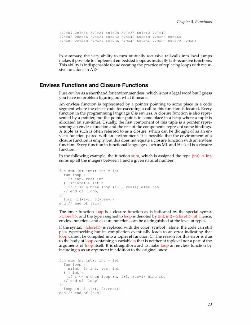
In the following example, the function sum, which is assigned the type (int) -> int,sums up all the integers between 1 and a given natural number:
fun sum (n: int): int = letfun loop (i: int, res: int
) :<cloref1> int =if i <= n then loop (i+1, res+i) else res
// end of [loop]inloop (1(*i*), 0(*res*))
end // end of [sum]
The inner function loop is a closure function as is indicated by the special syntax:<cloref1>, and the type assigned to loop is denoted by (int, int) -<cloref1> int. Hence,envless functions and closure functions can be distinguished at the level of types.
If the syntax :<cloref1> is replaced with the colon symbol : alone, the code can stillpass typechecking but its compilation eventually leads to an error indicating thatloop cannot be compiled into a toplevel function C. The reason for this error is dueto the body of loop containing a variable n that is neither at toplevel nor a part of thearguments of loop itself. It is straightforward to make loop an envless function byincluding n as an argument in addition to the original ones:
fun sum (n: int): int = letfun loop (n:int, i: int, res: int
) : int =if i <= n then loop (n, i+1, res+i) else res
// end of [loop]inloop (n, 1(*i*), 0(*res*))
end // end of [sum]
23

Chapter 3. Functions
As a matter of fact, what happens during compilation is that the first implementationof sum and loop gets translated, more or less, into the second implementation, andthere is simply no creation of closures (for representing closure functions) at run-time.
The need for creating closures often appears when the return value of a function callis a function itself. For instance, the following defined function addx returns anotherfunction when applied to a given integer x, and the returned function is a closurefunction, which always adds the integer x to its own argument:
fun addx (x: int): int -<cloref1> int = lam y => x + y
val plus1 = addx (1) // [plus1] is of the type int -<cloref1> intval plus2 = addx (2) // [plus2] is of the type int -<cloref1> int
It should be clear that plus1(0) and plus2(0) return 1 and 2, respectively. The closurethat is assigned the name plus1 consists of an envless function and an environmentbinding x to 1. The envless function can essentially be described by the pseudo syntaxlam (env, y) => env.x + y, where env and env.x refer to an environment and the valueto which x is bound in that environment. When evaluating plus1(0), we can first bindenv and y to the environment in plus1 and the argument 0, respectively, and thenstart to evaluate the body of the envless function in plus1, which is env.x + y. Clearly,this evaluation yields the value 1 as is expected.
Closures are often passed as arguments to functions that are referred to as higher-order functions. It is also not uncommon for closures to be embedded in data struc-tures.
Higher-Order FunctionsA higher-order function is a function that take another function as its argument. Forinstance, the following defined function rtfind is a higher-order one:
fun rtfind(f: int -> int): int = letfun loop (f: int -> int, n: int
) : int =if f(n) = 0 then n else loop (f, n+1)
// end of [loop]inloop (f, 0)
end // end of [rtfind]
Given a function from integers to integers, rtfind searches for the first natural numberthat is a root of the function. For instance, calling rtfind on the polynomial functionlam x => x * x - x + 110 returns 11. Note that rtfind loops forever if it is applied to afunction that does not have a root.
Higher-order functions can greatly facilitate code reuse, and I now present a simpleexample to illustrate this point. The following defined functions sum and prod com-pute the sum and product of the integers ranging from 1 to a given natural number,respectively:
fun sum (n: int): int = if n > 0 then sum (n-1) + n else 0fun prod (n: int): int = if n > 0 then prod (n-1) * n else 1
The similarity between the functions sum and prod is evident. We can define ahigher-function ifold and then implement sum and prod based on ifold:
fun ifold
24

Chapter 3. Functions
(n: int, f: (int, int) -> int, ini: int): int =if n > 0 then f (ifold (n-1, f, ini), n) else ini
// end of [ifold]
fun sum (n: int): int = ifold (n, lam (res, x) => res + x, 0)fun prod (n: int): int = ifold (n, lam (res, x) => res * x, 1)
If we ever want to compute the sum of the squares of the integers ranging from 1 toa given natural number, we can readily define a function based on ifold to do it:
fun sqrsum (n: int): int = ifold (n, lam (res, x) => res + x * x, 0)
As more features of ATS are introduced, higher-order functions will become evenmore effective in facilitating code reuse.
Example: Binary SearchWhile binary search is often performed on an ordered array to check whether a givenelement is stored in that array, it can also be employed to compute the inverse ofan increasing or decreasing function on integers. In the following code, the definedfunction bsearch_fun returns an integer i0 such that f(i) <= x0 holds for i rangingfrom lb to i, inclusively, and x0 < f(i) holds for i ranging from i+1 to ub, inclusively:
//// The type [uint] is for unsigned integers//fun bsearch_fun (f: int -<cloref1> uint
, x0: uint, lb: int, ub: int) : int =if lb <= ub then letval mid = lb + (ub - lb) / 2
inif x0 < f (mid) thenbsearch_fun (f, x0, lb, mid-1)
elsebsearch_fun (f, x0, mid+1, ub)
// end of [if]end else ub // end of [if]
// end of [bsearch_fun]
As an example, the following function isqrt is defined based on bsearch_fun to com-pute the integer square root of a given natural number, that is, the largest integerwhose square is less than or equal to the given natural number:
//// Assuming that [uint] is of 32 bits//val ISQRT_MAX = (1 << 16) - 1 // = 65535fun isqrt (x: uint): int =bsearch_fun (lam i => square ((uint_of_int)i), x, 0, ISQRT_MAX)
// end of [isqrt]
Note that the function uint_of_int is for casting a signed integer into an unsignedinteger and the function square returns the square of its argument.
Please find the entire code in this section plus some additional code for testing on-line4.
25
Chapter 3. Functions
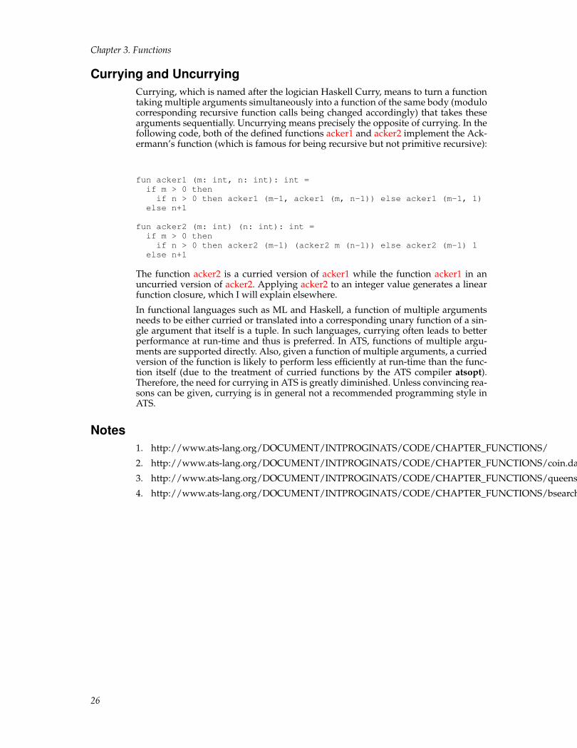
Currying and UncurryingCurrying, which is named after the logician Haskell Curry, means to turn a functiontaking multiple arguments simultaneously into a function of the same body (modulocorresponding recursive function calls being changed accordingly) that takes thesearguments sequentially. Uncurrying means precisely the opposite of currying. In thefollowing code, both of the defined functions acker1 and acker2 implement the Ack-ermann’s function (which is famous for being recursive but not primitive recursive):
fun acker1 (m: int, n: int): int =if m > 0 thenif n > 0 then acker1 (m-1, acker1 (m, n-1)) else acker1 (m-1, 1)
else n+1
fun acker2 (m: int) (n: int): int =if m > 0 thenif n > 0 then acker2 (m-1) (acker2 m (n-1)) else acker2 (m-1) 1
else n+1
The function acker2 is a curried version of acker1 while the function acker1 in anuncurried version of acker2. Applying acker2 to an integer value generates a linearfunction closure, which I will explain elsewhere.
In functional languages such as ML and Haskell, a function of multiple argumentsneeds to be either curried or translated into a corresponding unary function of a sin-gle argument that itself is a tuple. In such languages, currying often leads to betterperformance at run-time and thus is preferred. In ATS, functions of multiple argu-ments are supported directly. Also, given a function of multiple arguments, a curriedversion of the function is likely to perform less efficiently at run-time than the func-tion itself (due to the treatment of curried functions by the ATS compiler atsopt).Therefore, the need for currying in ATS is greatly diminished. Unless convincing rea-sons can be given, currying is in general not a recommended programming style inATS.
Notes1. http://www.ats-lang.org/DOCUMENT/INTPROGINATS/CODE/CHAPTER_FUNCTIONS/
2. http://www.ats-lang.org/DOCUMENT/INTPROGINATS/CODE/CHAPTER_FUNCTIONS/coin.dats
3. http://www.ats-lang.org/DOCUMENT/INTPROGINATS/CODE/CHAPTER_FUNCTIONS/queens.dats
4. http://www.ats-lang.org/DOCUMENT/INTPROGINATS/CODE/CHAPTER_FUNCTIONS/bsearch.dats
26

Chapter 4. Datatypes
A datatype is like a tagged union type. For each datatype, there are some constructorsassociated with it, and these constructors are needed for constructing values of thedatatype. As an example, the following syntax declares a datatype named intopt:
datatype intopt =| intopt_none of () | intopt_some of (int)
// end of [intopt]
There are two constructors associated with intopt: intopt_none, which is nullary, andintopt_some, which is unary. For instance, intopt_none() and intopt_some(1) are twovalues of the type intopt. In order for accessing components in such values, a mech-anism often referred to as pattern-matching is provided in ATS. I will demonstratethrough examples that datatypes plus pattern matching can offer not only great con-venience in programming but also clarity in code.
The code employed for illustration in this chapter plus some additional code for test-ing is available on-line1.
PatternsPatterns in ATS can be defined inductively as follows:
• Certain constant values such booleans, chars, floating point numbers, integers andstrings are patterns.
• The void value () is a pattern.
• The underscore symbol _ represents a special wildcard pattern.
• Variables are patterns.
• A tuple of patterns, either boxed or unboxed, is a pattern.
• A record of patterns, either boxed or unboxed, is a pattern.
• Given a constructor C, a pattern can be formed by applying C to a given list ofpatterns.
• Given a variable x and a pattern pat, (x as pat) is a referenced pattern, where as isa keyword.
• Some other forms of patterns will be introduced elsewhere.
Each variable can occur at most once in a given pattern, and this is referred as thelinearity restriction on variables in patterns. For instance, (x, x) is not a legal patternas the variable x appears twice in it. However, this restriction does not apply to thevariable _, which represents the wildcard pattern.
Pattern-MatchingPattern matching means matching values against patterns. In the case where a valuematches a pattern, a collection of bindings are generated between the variables in thepattern and certain components in the value. Pattern-matching is performed accord-ing to the following set of rules:
• A value that matches a constant pattern must be the same constant, and this match-ing generates no bindings.
• The void value () only matches the pattern (), and this matching generate no bind-ings.
27
Chapter 4. Datatypes
• Any value can match the wildcard pattern, and this matching generates no bind-ings.
• Any value can match a variable pattern, and this matching generates a bindingbetween the variable and the value.
• A tuple value matches a tuple pattern if they are of the same length and each valuecomponent in the former matches the corresponding pattern component in thelatter, and this matching generates a collection of bindings that is the union ofthe bindings generated from matching the value components in the tuple valueagainst the pattern components in the tuple pattern.
• A record value matches a record pattern if they have the same field names and eachvalue component in the former matches the corresponding pattern component inthe latter, and this matching generates a collection of bindings that is the union ofthe bindings generated from matching the value components in the record valueagainst the pattern components in the record pattern.
• Given a pattern formed by applying a constructor C to some pattern arguments,a value matches this pattern if the value is formed by applying C to some valuearguments matching the pattern arguments, and this matching generates a collec-tion of bindings that is the union of the binding generated from matching the valuearguments against the pattern arguments.
• Given a referenced pattern (x as pat), a value matches the pattern if it matchespat, and this matching generates a collection of bindings that extends the bindingsgenerated from matching the value against pat with a binding from x to the value.
Suppose we have a tuple value (0, 1, 2, 3) and a tuple pattern (1, _, x, y). Then thevalue matches the pattern and this matching yields bindings from x and y to 2 and 3,respectively.
Matching Clauses and Case-ExpressionsGiven a pattern pat and an expression exp, (pat => exp) is a matching clause. Thepattern pat and the expression exp are referred to as the guard and the body of thematching clause.
Given an expression exp0 and a sequence of matching clauses clseq, a case-expressioncan be formed as such: (case exp0 of clseq). To evaluate the case-expression under agiven environment ENV0, we first evaluate exp0 under ENV0 to a value. If this valuedoes not match the guard of any clause in clseq, then the evaluation of the case-expression aborts. Otherwise, we choose the first clause in clseq such that the valuematches its guard. Let ENV1 be the environment that extends ENV0 with the bind-ings generated from this matching, and we evaluate the body of the chosen clauseunder ENV1. The value of obtained from this evaluation is the value of the case-expression we started to evaluate.
Enumerative DatatypesThe simplest form of datatypes is for enumerating a finite number of constants. Forinstance, the following concrete syntax introduces a datatype of the name wday:
datatype wday =| Monday of ()| Tuesday of ()| Wednesday of ()| Thursday of ()| Friday of ()| Saturday of ()| Sunday of ()
28

Chapter 4. Datatypes
// end of [wday]
where the first bar symbol (|) is optional. There are 7 nullary constructors introducedin the datatype declaration: Monday through Sunday, which are for constructing val-ues of the type wday. For instance, Monday() is a value of the type wday. Given anullary constructor C, we can write C for C() as a value. For instance, we can writeMonday for Monday(). However, one should not assume that Tuesday is somethinglike Monday+1.
The following code implements a function that tests whether a given value of thetype wday is a weekday or not:
fun isWeekday(x: wday): bool = case x of| Monday () => true // the bar (|) is optional for the first clause| Tuesday () => true| Wednesday () => true| Thursday () => true| Friday () => true| Saturday () => false| Sunday () => false
// end of [isWeekday]
Given a unary constructor C, C() is a pattern that can only match the value C(). Notethat C() cannot be written as C when it is used as a pattern. If Monday () is writtenas Monday in the body of the function isWeekday, then an error message is to bereported during typechecking, indicating that all the clauses after the first one areredundant. This is simply due to Monday being treated as a variable pattern, whichis matched by any value. A likely more sensible implementation of isWeekday isgiven as follows:
fun isWeekday(x: wday): bool = case x of| Saturday () => false | Sunday () => false | _ => true
// end of [isWeekday]
This implementation works because pattern-matching is done sequentially at run-time: If a value of the type wday does not match either of Saturday () and Sunday (),then it must match one of Monday () , Tuesday () , Wednesday () , Thursday () andFriday ().
Recursive DatatypesA recursive datatype is one such that its associated constructors may form valuesby applying to values of the datatype itself. For instance, the following declareddatatype charlst is recursive:
datatype charlst =| charlst_nil of () | charlst_cons of (char, charlst)
When applied to a character and a value of the type charlst, the constructorcharlst_cons forms a value of the type charlst. As an example, the following valuerepresents a character list consisting of ’a’, ’b’ and ’c’:
char_cons (’a’, char_cons (’b’, char_cons (’c’, char_nil ())))
We can define a function charlst_length as follows to compute the length of a givencharacter list:
29

Chapter 4. Datatypes
fun charlst_length (cs: charlst): int =case cs of| charlst_cons (_, cs) => 1 + charlst_length (cs)| charlst_nil () => 0
// end of [charlst_length]
Note that this implementation is recursive but not tail-recursive. By relying on thecommutativity and associativity of integer addition, we can give the following im-plementation of charlst_length that is tail-recursive:
fun charlst_length(cs: charlst): int = letfun loop (cs: charlst, n: int): int = case cs of| charlst_cons (_, cs) => loop (cs, n+1) | charlst_nil () => n
// end of [loop]inloop (cs, 0)
end // end of [charlst_length]
Only a tail-recursive function should be given a name that suggests it is a loop. Thisis a naming convention I follow closely in this book and elsewhere.
Exhaustiveness of Pattern-MatchingGiven a type T and a set of patterns, if for any given value of the type T there is alwaysat least one pattern in the set such that the value matches the pattern, then pattern-matching values of the type T against the set of patterns is exhaustive. Given a case-expression of the form (case exp0 of clseq), where exp0 is assumed to be of sometype T, if pattern-matching values of the type T against the guards of the matchingclauses in clseq is exhaustive, then the case-expression is said to be pattern-matching-exhaustive.
The following code implements a function that finds the last character in a non-emptycharacter list:
fun charlst_last(cs: charlst): char = case cs of| charlst_cons (c, charlst_nil ()) => c| charlst_cons (_, cs1) => charlst_last (cs1)
// end of [charlst_last]
The body of charlst_last is a case-expression, which is not pattern-matching-exhaustive: If cs is bound to the value charlst_nil(), that is, the empty character list,than none of the matching clauses in the case-expression can be chosen. Whenthe code is typechecked by atsopt, a warning message is issued to indicate thecase-expression being non-pattern-matching-exhaustive. If the programmer wantsan error message instead, the keyword case should be replaced with case+. If theprogrammer wants to suppress the warning message, the keyword case should bereplaced with case-. I myself mostly use case+ when coding in ATS.
The function charlst_last can also be implemented as follows:
fun charlst_last(cs: charlst): char = case cs of| charlst_cons (c, cs1) => (case+ cs1 of
charlst_nil () => c | charlst_cons _ => charlst_last (cs1)) // end of [char_cons]
// end of [charlst_last]
In this implementation, the outer case-expression is not pattern-matching-exhaustivewhile the inner one is. Note that the pattern charlst_cons _ is just a shorthand for
30

Chapter 4. Datatypes
charlst_cons (_, _). In general, a pattern of the from (C _), where C is a constructor,can be matched by any value that is constructed by applying C to some values. Forinstance, the pattern charlst_nil () can also be written as charlst_nil _.
Suppose we have a case-expression containing only one matching clause, that is, thecase-expression is of the form (case exp0 of pat => exp). Then we can also write thiscase-expression as a let-expression: (let val pat = exp0 in exp end). For instance, wegive another implementation of the function charlst_last as follows:
fun charlst_last(cs: charlst): char = letval charlst_cons (c, cs1) = cs in case+ cs1 of| charlst_nil () => c | charlst_cons _ => charlst_last (cs1)
end // end of [charlst_last]
When this implementation is typechecked by atsopt, a warning message is issued toindicate the val-declaration being non-pattern-matching-exhaustive. If the program-mer wants an error message instead, the keyword val should be replaced with val+.If the programmer wants to suppress the warning message, the keyword val shouldbe replaced with val-.
As values formed by the constructors charlst_nil and charlst_cons are assigned thesame type charlst, it is impossible to rely on typechecking to prevent the functioncharlst_last from being applied to an empty character list. This is a serious limitation.With dependent types, which allow data to be described much more precisely, wecan ensure at the level of types that a function finding the last element of a list canonly be applied to a non-empty list.
Example: Evaluating Integer ExpressionsFor representing integer expressions, we declare a datatype IEXP as follows:
datatype IEXP =| IEXPnum of int // numeral| IEXPneg of (IEXP) // negative| IEXPadd of (IEXP, IEXP) // addition| IEXPsub of (IEXP, IEXP) // subtraction| IEXPmul of (IEXP, IEXP) // multiplication| IEXPdiv of (IEXP, IEXP) // division
// end of [IEXP]
The meaning of the constructors associated with IEXP should be obvious. A value ofthe type IEXP is often referred to as an abstract syntax tree. For instance, the abstractsyntax tree for the expression (~1+(2-3)*4) is the following one:
IEXPadd(IEXPneg(IEXPnum(1)), IEXPmul(IEXPsub(IEXPnum(2), IEXP(3)), IEXP(4)))
Translating an integer expression written in some string form into an abstract syntaxtree is called parsing, which we will not do here. The following defined functioneval_iexp takes the abstract syntax tree of an integer expression and return an integerthat is the value of the expression:
fun eval_iexp (e0: IEXP): int = case+ e0 of| IEXPnum n => n| IEXPneg (e) => ~eval_iexp (e)| IEXPadd (e1, e2) => eval_iexp (e1) + eval_iexp (e2)| IEXPsub (e1, e2) => eval_iexp (e1) - eval_iexp (e2)| IEXPmul (e1, e2) => eval_iexp (e1) * eval_iexp (e2)| IEXPdiv (e1, e2) => eval_iexp (e1) / eval_iexp (e1)
31

Chapter 4. Datatypes
// end of [eval_iexp]
Suppose we also allow the construct if-then-else to be use in forming integer expres-sions. For instance, we may write an integer expression like (if 1+2 <= 3*4 then 5+6else 7-8). Note that the test (1+2 <= 3*4) is a boolean expression rather than an integerexpression. This indicates that we also need to declare a datatype BEXP for represent-ing boolean expressions. Furthermore, IEXP and BEXP should be defined mutuallyrecursively, which is shown in the following code:
datatype IEXP =| IEXPcst of int // integer constants| IEXPneg of (IEXP) // negative| IEXPadd of (IEXP, IEXP) // addition| IEXPsub of (IEXP, IEXP) // subtraction| IEXPmul of (IEXP, IEXP) // multiplication| IEXPdiv of (IEXP, IEXP) // division| IEXPif of (BEXP(*test*), IEXP(*then*), IEXP(*else*))
// end of [IEXP]
and BEXP = // [and] for combining datatype declarations| BEXPcst of bool // boolean constants| BEXPneg of BEXP // negation| BEXPconj of (BEXP, BEXP) // conjunction| BEXPdisj of (BEXP, BEXP) // disjunction| BEXPeq of (IEXP, IEXP) // equal-to| BEXPneq of (IEXP, IEXP) // not-equal-to| BEXPlt of (IEXP, IEXP) // less-than| BEXPlte of (IEXP, IEXP) // less-than-equal-to| BEXPgt of (IEXP, IEXP) // greater-than| BEXPgte of (IEXP, IEXP) // greater-than-equal-to
// end of [BEXP]
Evidently, we also need to evaluate boolean expressions when evaluating integerexpressions. The following two functions eval_iexp and eval_bexp for evaluating in-teger and boolean expressions, respectively, are defined mutually recursively as isexpected:
fun eval_iexp (e0: IEXP): int = case+ e0 of| IEXPcst n => n| IEXPneg (e) => ~eval_iexp (e)| IEXPadd (e1, e2) => eval_iexp (e1) + eval_iexp (e2)| IEXPsub (e1, e2) => eval_iexp (e1) - eval_iexp (e2)| IEXPmul (e1, e2) => eval_iexp (e1) * eval_iexp (e2)| IEXPdiv (e1, e2) => eval_iexp (e1) / eval_iexp (e1)| IEXPif (e_test, e_then, e_else) => let
val b = eval_bexp (e_test) in eval_iexp (if b then e_then else e_else)end // end of [IEXPif]
// end of [eval_iexp]
and eval_bexp (e0: BEXP): bool = case+ e0 of| BEXPcst b => b| BEXPneg (e) => ~eval_bexp (e)| BEXPconj (e1, e2) => if eval_bexp (e1) then eval_bexp (e2) else false| BEXPdisj (e1, e2) => if eval_bexp (e1) then true else eval_bexp (e2)| BEXPeq (e1, e2) => eval_iexp (e1) = eval_iexp (e2)| BEXPneq (e1, e2) => eval_iexp (e1) <> eval_iexp (e2)| BEXPlt (e1, e2) => eval_iexp (e1) < eval_iexp (e2)| BEXPlte (e1, e2) => eval_iexp (e1) <= eval_iexp (e2)| BEXPgt (e1, e2) => eval_iexp (e1) > eval_iexp (e2)| BEXPgte (e1, e2) => eval_iexp (e1) >= eval_iexp (e2)
// end of [eval_bexp]
32

Chapter 4. Datatypes
The integer and boolean expressions used in this example are all constant expressionscontaining no variables. Therefore, there is no need for an environment to evaluatethem. I will present a more advanced example elsewhere to demonstrate how anevaluator for a simple call-by-value functional programming language like the coreof ATS can be implemented.
Notes1. http://www.ats-lang.org/DOCUMENT/INTPROGINATS/CODE/CHAPTER_DATATYPES/
33

Chapter 4. Datatypes
34

Chapter 5. Parametric Polymorphism
Code sharing is of paramount importance in programming language design. In atyped programming language, we often encounter a situation where the same func-tionality is needed for values of different types. For instance, we need a function tocompute the length of a list while the elements in the list may be characters, integers,strings, etc. Evidently, we want to avoid implementing such a function for each el-ement type as it would probably be the worst form of code duplication otherwise.We want to implement a single function that can be applied to any list to computethe length of the list. The length-computing function parameterizes over the elementtype of a list it is applied to, and it behaves uniformly regardless what the elementtype is. This is a form of code sharing that is given the name: parametric polymor-phism, which should be distinguished from other forms of polymorphism such asinheritance polymorphism in object-oriented programming.
The code employed for illustration in this chapter plus some additional code for test-ing is available on-line1.
Function TemplatesA function template is a code template that implements a function. In the followingcode, two functions are defined to swap values:
typedef charint = (char, int)typedef intchar = (int, char)fun swap_char_int (xy: charint): intchar = (xy.1, xy.0)fun swap_int_char (xy: intchar): charint = (xy.1, xy.0)
If types are ignored, the bodies of swap_char_int and swap_int_char are identical. Inorder to avoid this kind of code duplication, we can first implement a function tem-plate swap as follows and then implement swap_char_int and swap_int_char basedon swap:
fun{a,b:t@ype} swap (xy: (a, b)): (b, a) = (xy.1, xy.0)fun swap_char_int (xy: charint): intchar = swap<char,int> (xy)fun swap_int_char (xy: intchar): charint = swap<int,char> (xy)
It should be noted that a function template is not a first-class value in ATS: There isno expression for representing a function template. The syntax {a,b:t@ype} followingthe keyword fun represents template parameters or arguments. The unusual symbolt@ype is a sort for static terms representing types of unspecified size, where the sizeof a type is the number of bytes needed for representing a value of the type. There isanother sort type in ATS, which is for static terms representing types of size equal toone word exactly, that is, 4 bytes on a 32-bit machine or 8 bytes on a 64-bit machine.The syntax swap<char,int>, where no space is allowed between swap and < , standsfor an instance of the function template swap in which the parameters a and b arereplaced with char and int, respectively. The syntax swap<int,char> is interpretedsimilarly.
A different style of implementation of swap is given as follows:
fun{a:t@ype}{b:t@ype} swap2 (xy: (a, b)): (b, a) = (xy.1, xy.0)
where the template parameters are given sequentially (instead of simultaneously).The following code shows how swap2 can be instantiated to for instances:
fun swap_char_int (xy: charint): intchar = swap2<char><int> (xy)fun swap_int_char (xy: intchar): charint = swap2<int><char> (xy)
35

Chapter 5. Parametric Polymorphism
Note that >< is a special symbol (of the name GTLT) and no space is allowed between> and <.
As another example, a higher-order function template for composing (closure) func-tions is given as follows:
typedef cfun (t1:t@ype, t2:t@ype) = t1 -<cloref1> t2
fun{a,b,c:t@ype} compose(f: cfun (a, b), g: cfun (b, c)):<cloref1> cfun (a, c) = lam x => g(f(x))
// end of [compose]
val plus1 = lam (x:int): int =<cloref1> x+1val times2 = lam (x:int): int =<cloref1> x*2
val f_2x_1: cfun (int, int) = compose (times2, plus1)val f_2x_2: cfun (int, int) = compose (plus1, times2)
It should be clear that the value f_2x_1 represents the function that multiplies itsinteger argument by 2 and then adds 1 to it. Similarly, the value f_2x_2 represents thefunction that adds 1 to its integer argument and then multiplies it by 2.
In ATS, function templates are typechecked but not compiled. Only instances of afunction template can be compiled. Suppose we have a function template foo takingone type parameter and two instances foo<T1> and foo<T2> are used in a programfor some types T1 and T2. In general, one function in C is generated for each instanceof foo when the program is compiled. However, if T1 and T2 have the same name,then the two instances share one function in C. In particular, if both T1 and T2 areboxed types, which are always given the same name, only one function in C is gen-erated for them.
Please note that I may simply use the name function to refer to a function templatefrom now on if no confusion is expected.
Polymorphic FunctionsA polymorphic function is rather similar to a function template. However, the for-mer is a first-class value in ATS while the latter is not. As an example, the followingdefined function swap_boxed is polymorphic:
fun swap_boxed {a,b:type} (xy: (a, b)): (b, a) = (xy.1, xy.0)
The type variables a and b are often referred as static arguments while xy is a dy-namic argument. Here is some code that makes use of the polymorphic functionswap_boxed:
val AB = ("A", "B")val BA1 = swap_boxed {string,string} (AB) // [string] is boxedval BA2 = swap_boxed (AB) // this is fine, too
If swap_boxed is called on a pair of the type (T1, T2) for some types T1 and T2, bothT1 and T2 are required to be boxed. Otherwise, a type-error is reported. For instance,calling swap_boxed on (0, 1) yields a type-error as the type int is not boxed.
When calling a polymorphic function, we often omit passing static arguments ex-plicitly and expect them to be synthesized by the compiler. However, there are alsooccasions, which are not uncommon, where static arguments need to be supplied ex-plicitly as either they cannot be successfully synthesized or what is synthesized is notexactly what is expected.
36

Chapter 5. Parametric Polymorphism
It is also possible to pass static arguments sequentially as is shown in the followingstyle of implementation of a polymorphic function:
fun swap2_boxed {a:type} {b:type} (xy: (a, b)): (b, a) = (xy.1, xy.0)
val AB = ("A", "B")val BA1 = swap2_boxed {string} {string} (AB)val BA2 = swap2_boxed (AB) // this is fine, tooval BA3 = swap2_boxed {..} {string} (AB) // 1st static argument to be synthesizedval BA4 = swap2_boxed {string} {..} (AB) // 2nd static argument to be synthesizedval BA5 = swap2_boxed {..} {..} (AB) // both arguments to be synthesizedval BA6 = swap2_boxed {...} (AB) // every static argument to be synthesized
The special syntax {..} indicates to the typechecker that the static argument (or argu-ments) involved in the current application should be synthesized while the specialsyntax {...} means that the rest of static arguments should all be synthesized.
I have seen two kinds of errors involving polymorphic functions that are extremelycommon in practice.
• The first kind is depicted in the following example:
fun swap_boxed {a,b:t@ype} (xy: (a, b)): (b, a) = (xy.1, xy.0)
Notice that the sort for type variables a and b is t@ype (instead of type). Whilethis example can pass typechecking, its compilation results in an error that mayseem mysterious to many programmers. The simple reason for this error is thatthe compiler cannot figure out the size of a and b when trying to generate code inC as the sort t@ype is for types of unspecified size.
• The second kind is depicted in the following example:
fun{a,b:type} swap_boxed (xy: (a, b)): (b, a) = (xy.1, xy.0)
Strictly speaking, there is really no error in this case. If defined as such,swap_boxed is a function template instead of a polymorphic function. However,such a function template is severely restricted as it cannot be instantiated withtypes that are not boxed. While this could be intended, it is likely not.
Given the potential confusion, why do we need both function templates and poly-morphic functions? At this stage, it is certainly plausible that we program only withfunction templates and make no use of polymorphic functions. However, polymor-phic functions can hardly be missed in the presence dependent types. There will ac-tually be numerous occasions where we encounter polymorphic function templates,that is, templates for polymorphic functions.
Polymorphic DatatypesCode sharing also applies to datatype declarations. For instance, a commonly usedpolymorphic datatype list0 is declared as follows:
datatype list0 (a:t@ype) =| list0_nil (a) of () | list0_cons (a) of (a, list0 a)
// end of [list0]
More precisely, list0 is a type constructor. Given a type T, we can form a type list0(T)for lists consisting of elements of the type T. For instance, list0(char) is for characterlists, list0(int) for integer lists, list0(list0(int)) for lists whose elements themselves areinteger lists, etc. To a great extent, the need for function templates or polymorphic
37

Chapter 5. Parametric Polymorphism
functions largely stems from the availability of polymorphic datatypes. As an exam-ple, a function template list0_length is implemented as follows for computing thelength of any given list:
fun{a:t@ype}list0_length (xs: list0 a): int = case+ xs of| list0_cons (_, xs) => 1 + list0_length (xs) | list0_nil () => 0
// end of [list0_length]
When applying list0_length to a list xs, we can in general write list0_length(xs), ex-pecting the typechecker to synthesize a proper type parameter for list0_length. Wemay also write list0_length<T>(xs) if the elements of xs are of the type T. The latterstyle, though a bit more verbose, is likely to yield more informative messages in casetype-errors occur.
Another commonly used polymorphic datatype option0 is declared as follows:
datatype option0 (a:t@ype) =| option0_none (a) of () | option0_some (a) of a
// end of [option0]
A typical use of option0 is to perform some kind of error-handling. Suppose that weare to implement a function doing integer division and we want to make sure thatthe function returns even if it is called in a case where the divisor equals 0. This canbe done as follows:
fun divopt (x: int, y: int): option0 (int) =if y = 0 then option0_none () else option0_some (x/y)
// end of [divopt]
By inspecting what divopt returns, we can tell whether integer division has beendone normally or an error of divsion-by-zero has occurred. A realistic use of option0is shown in the following implementation of list0_last:
fun{a:t@ype}list0_last (xs: list0 a): option0 (a) = letfun loop (x: a, xs: list0 a): a = case+ xs of| list0_nil () => x | list0_cons (x, xs) => loop (x, xs)
// end of [loop]incase+ xs of| list0_nil () => option0_none ()| list0_cons (x, xs) => option0_some (loop (x, xs))
end // end of [list0_last]
When applied to a list, list0_last returns an optional value. If the value matches thepattern option0_none(), then the list is empty. Otherwise, the value is formed by ap-plying option0_some to the last element in the list.
Example: Function Templates on ListsIn functional programming, lists are ubiquitous. We implement as follows some com-monly used function templates on lists. It should be noted that these templates areall available in a library of ATS, where they may be implemented in a significantlymore efficient manner due to the use of certain programming features that have notbeen covered so far.
Please find the entire code in this section plus some additional code for testing on-line2.
38
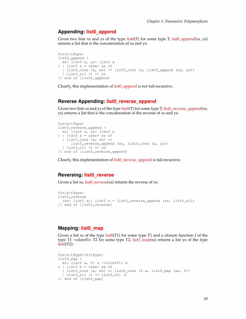
Chapter 5. Parametric Polymorphism
Appending: list0_appendGiven two lists xs and ys of the type list0(T) for some type T, list0_append(xs, ys)returns a list that is the concatenation of xs and ys:
fun{a:t@ype}list0_append (xs: list0 a, ys: list0 a
) : list0 a = case+ xs of| list0_cons (x, xs) => list0_cons (x, list0_append (xs, ys))| list0_nil () => ys
// end of [list0_append]
Clearly, this implementation of list0_append is not tail-recursive.
Reverse Appending: list0_reverse_appendGiven two lists xs and ys of the type list0(T) for some type T, list0_reverse_append(xs,ys) returns a list that is the concatenation of the reverse of xs and ys:
fun{a:t@ype}list0_reverse_append (xs: list0 a, ys: list0 a
) : list0 a = case+ xs of| list0_cons (x, xs) =>
list0_reverse_append (xs, list0_cons (x, ys))| list0_nil () => ys
// end of [list0_reverse_append]
Clearly, this implementation of list0_reverse_append is tail-recursive.
Reversing: list0_reverseGiven a list xs, list0_reverse(xs) returns the reverse of xs:
fun{a:t@ype}list0_reverse(xs: list0 a): list0 a = list0_reverse_append (xs, list0_nil)
// end of [list0_reverse]
Mapping: list0_mapGiven a list xs of the type list0(T1) for some type T1 and a closure function f of thetype T1 -<cloref1> T2 for some type T2, list0_map(xs) returns a list ys of the typelist0(T2):
fun{a:t@ype}{b:t@ype}list0_map (xs: list0 a, f: a -<cloref1> b
) : list0 b = case+ xs of| list0_cons (x, xs) => list0_cons (f x, list0_map (xs, f))| list0_nil () => list0_nil ()
// end of [list0_map]
39

Chapter 5. Parametric Polymorphism
The length of ys equals that of xs and each element y in ys equals f(x), where x isthe corresponding element in xs. Clearly, this implementation of list0_map is not tail-recursive.
Zipping: list0_zipGiven two lists xs and ys of the types list0(T1) and list0(T2) for some types T1 andT2, respectively, list0_zip(xs, ys) returns a list zs of the type list0 @(T1, T2):
fun{a,b:t@ype}list0_zip (xs: list0 a, ys: list0 b
) : list0 @(a, b) = case+ (xs, ys) of| (list0_cons (x, xs),
list0_cons (y, ys)) => list0_cons ((x, y), list0_zip (xs, ys))| (_, _) => list0_nil ()
// end of [list0_zip]
The length of zs is the minimum of the lengths of xs and ys and each element z inzs @(x, y), where x and y are the corresponding elements in xs and ys, respectively.Clearly, this implementation of list0_zip is not tail-recursive.
Zipping with: list0_zipwithGiven two lists xs and ys of the types list0(T1) and list0(T2) for some types T1 andT2, respectively, and a closure function f of the type (T1, T2) -<cloref1> T3 for sometype T3, list0_zipwith(xs, ys, f) returns a list zs of the type list0(T3):
fun{a,b:t@ype}{c:t@ype}list0_zipwith (xs: list0 a
, ys: list0 b, f: (a, b) -<cloref1> c) : list0 c = case+ (xs, ys) of| (list0_cons (x, xs), list0_cons (y, ys)) =>
list0_cons (f (x, y), list0_zipwith (xs, ys, f))| (_, _) => list0_nil ()
// end of [list0_zipwith]
The length of zs is the minimum of the lengths of xs and ys and each element zin zs is f(x, y), where x and y are the corresponding elements in xs and ys, respec-tively. Clearly, this implementation of list0_zipwith is not tail-recursive. Note thatlist0_zipwith behaves exactly like list0_zip if its third argument f is replaced withlam (x, y) => @(x, y). This function template is also named list0_map2 for the obviousreason.
Example: Mergesort on ListsMergesort is simple sorting algorithm that is guaranteed to be log-linear. It is stablein the sense that the order of two equal elements always stay the same after sorting.I give as follows a typical functional style of implementation of mergesort on lists.
First, let us introduce abbreviations for the list constructors list0_nil and list0_cons:
#define nil list0_nil // writing [nil] for list0_nil#define :: list0_cons // writing [::] for list0_cons#define cons list0_cons // writing [cons] for list0_cons
40
Chapter 5. Parametric Polymorphism
Note that the operator :: is already given the infix status. For instance, the list consist-ing of the first 5 natural numbers can be constructed as follows:
cons (0, cons (1, 2 :: 3 :: 4 :: nil ()))
In practice, there is of course no point in mixing cons with ::.
We next implement a function template merge to merge two given ordered lists intoa single ordered one:
typedef lte (a:t@ype) = (a, a) -> bool
fun{a:t@ype}merge (xs: list0 a, ys: list0 a, lte: lte a
) : list0 a =case+ xs of| x :: xs1 => (case+ ys of| y :: ys1 =>
if x \lte y thenx :: merge (xs1, ys, lte))
elsey :: merge (xs, ys1, lte))
// end of [if]| nil () => xs) // end of [::]
| nil () => ys// end of [merge]
For instance, suppose that the two given lists are (1, 3, 4, 8) and (2, 5, 6, 7, 9), andthe comparison function (the third argument of merge) is the standard less-than-or-equal-to function on integers. Then the list returned by merge is (1, 2, 3, 4, 5, 6, 7, 8,9). The syntax \lte means that the particular occurrence of lte following the backslashsymbol (\) is given the infix status, and thus the expression x \lte y means the sameas lte(x, y).
The following function template mergesort implements the standard mergesort algo-rithm:
fun{a:t@ype}mergesort(xs: list0 a, lte: lte a): list0 a = let
//fun msort (xs: list0 a, n: int, lte: lte a
) : list0 a =if n >= 2 then split (xs, n, lte, n/2, nil) else xs
and split (xs: list0 a, n: int, lte: lte a, i: int, xsf: list0 a
) : list0 a =if i > 0 then letval- cons (x, xs) = xs
insplit (xs, n, lte, i-1, cons (x, xsf))
end else letval xsf = list0_reverse<a> (xsf) // make sorting stable!val xsf = msort (xsf, n/2, lte) and xs = msort (xs, n-n/2, lte)
inmerge (xsf, xs, lte)
end // end of [if]//val n = list0_length<a> (xs)
//
41

Chapter 5. Parametric Polymorphism
inmsort (xs, n, lte)
end // end of [mergesort]
Suppose we want to sort the list (8, 3, 4, 1, 2, 7, 6, 5, 9); we first divide it into two lists:(8, 3, 4, 1) and (2, 7, 6, 5, 9); by performing mergesort on each of them, we obtain twoordered lists: (1, 3, 4, 8) and (2, 5, 6, 7, 9); by merging these two ordered list, we obtainthe ordered list (1, 2, 3, 4, 5, 6, 7, 8, 9), which is a permutation of the original one.
Note that the function template merge is not tail-recursive as the call to merge in itsbody is not a tail-call. This is a serious problem in practice: It is almost certain that astack overflow is to occur if the above implementation of mergesort is employed tosort a list that is very long (e.g., containing 1,000,000 elements or more). I will latergive a tail-recursive implementation of the merge function in ATS that makes use oflinear types.
Please find the entire code in this section plus some additional code for testing on-line3.
Notes1. http://www.ats-lang.org/DOCUMENT/INTPROGINATS/CODE/CHAPTER_POLYMORPHISM
2. http://www.ats-lang.org/DOCUMENT/INTPROGINATS/CODE/CHAPTER_POLYMORPHISM/listfun.dats
3. http://www.ats-lang.org/DOCUMENT/INTPROGINATS/CODE/CHAPTER_POLYMORPHISM/mergesort.dats
42

Chapter 6. Summary
I have given a presentation of the core of ATS in this part of book. While this coreis largely similar to the core of the functional language ML (and various other call-by-value functional languages), there are also crucial differences. I list some of thesedifferences as follows:
• ATS shares the same native data representation with the C programminglanguage. This differs profoundly from ML and most other functional languages,which all rely on some forms of boxed data representation. In ATS, there arenative/flat/unboxed tuples and records as well as boxed ones.
• ATS supports both envless functions and closure functions while ML and mostother functional languages only support the latter. In ATS, envless functions andclosure functions can be differentiated at the level of types.
• In ATS, there are both function templates and polymorphic functions. The need forthe former primarily stems from the need for handling native data representationdirectly.
• ATS provides explicit support for mutually recursive tail-call optimization.
Except for making a few uses of printing functions, I have intentionally stayed awayfrom programming features that can generate effects when presenting the core ofATS. I will cover such programming features when addressing in the next part of thebook the issue of supporting practical programming in ATS.
43
Chapter 6. Summary
44

Chapter 7. Effectful Programming Features
Effectful programming features are those that can generate effects at run-time. Butwhat is really an effect? The answer to this question is rather complex as it dependson the model of evaluation. I will gradually introduce various kinds of effects in thisbook. In sequential programming, that is, constructing programs to be evaluated se-quentially (in contrast to concurrently), an expression is effectless if there exists avalue such that the expression and the value cannot be distinguished as far as eval-uation is concerned. For instance, the expression 1+2 is effectless as it cannot be dis-tinguished from the value 3. An effectless expression is also said to be pure. On theother hand, an effectful expression is one that can be distinguished from any givenvalues. For instance, the expression print("Hello") is effectful as its evaluation resultsin an observable behavior that distinguishes the expression from any values. In thiscase, print("Hello") is said to contain certain I/O effect. If the evaluation of an expres-sion never terminates, then the expression is also effectul. For instance, let us definea function loop as follows:
fun loop (): void = loop ()
Then the expression loop() can be distinguished from any values in the followingcontext:
let val _ = [] in print ("Terminated") end
If the hole [] in the context is replaced with loop(), then the evaluation of the result-ing expression continues forever. If the hole [] is replaced with any value, then theevaluation leads to the string "Terminated" being printed out. The expression loop issaid to contain the non-termination effect.
I will cover programming features related to exceptional control-flow, persistentmemory storage and simple I/O in this chapter, which are all of common use inpractical programming.
The code employed for illustration in this chapter plus some additional code for test-ing is available on-line1.
ExceptionsThe exception mechanism provides an efficient means for reporting a special con-dition encountered during program evaluation. Often such a special condition indi-cates an error, but it is not uncommon to use the exception mechanism for addressingissues that are not related to errors.
The type exn is predefined in ATS. One may think of exn as an extensible datatypefor which new constructors can always be declared. For instance, two exception con-structors are declared as follows:
exception FatalError0 of ()exception FatalError1 of (string)
The constructor FatalError0 is nullary while the constructor FatalError1 is unary.Exception values, that is, values of the type exn can be formed by applyingexception constructors to proper arguments. For instance, FatalError0() andFatalError1("division-by-zero") are two exception values (or simply exceptions). Inthe following program, a function for integer division is implemented:
exception DivisionByZero of ()fun divexn (x: int, y: int): int =if y <> 0 then then x / y else $raise DivisionByZero()
45

Chapter 7. Effectful Programming Features
// end of [divexn]
When the function call divexn(1, 0) is evaluated, the exception DivisionByZero() israised. The keyword $raise in ATS is solely for raising exceptions.
A raise-expression is of the form ($raise exp) for some expression exp. Clearly, if theevaluation of exp returns a value, then the evaluation of ($raise exp) leads to a raisedexception. Therefore, the evaluation of a raise-expression can never return a value,and this justifies that a raise-expression can be given any type.
A raised exception can be captured. If it is not captured, the raised exception abortsthe program evaluation that issued it in the first place. In ATS, a try-expression is ofthe form (try exp with clseq), where try is a keyword, exp is an expression, with isalso a keyword, and clseq is a sequence of matching clauses. When evaluating sucha try-expression, we first evaluate exp. If the evaluation of exp leads to a value, thenthe value is also the value of the try-expression. If the evaluation of exp leads to araised exception, then we match the exception against the guards of the matchingclauses in clseq. If there is a match, the raised exception is caught and we continue toevaluate the body of the first clause whose guard is matched. If there is no match, theraised exception is uncaught. In a try-expression, the with-part is often referred to asan exception-handler.
Let us now see an example that involves raising and capturing an exception. In thefollowing program, three functions are defined to compute the product of the inte-gers in a given list:
fun listprod1(xs: list0 (int)): int = case+ xs of| list0_cons (x, xs) => x * listprod1 (xs) | list0_nil () => 1
// end of [listprod1]
fun listprod2(xs: list0 (int)): int = case+ xs of| list0_cons (x, xs) => if x = 0 then 0 else x * listprod2 (xs)| list0_nil () => 1
// end of [listprod2]
fun listprod3(xs: list0 (int)): int = letexception ZERO of ()fun aux (xs: list0 (int)): int =case+ xs of| list0_cons (x, xs) =>
if x = 0 then $raise ZERO() else x * aux (xs)| list0_nil () => 1
// end of [aux]intry aux (xs) with ~ZERO () => 0
end // end of [listprod3]
While these functions can all be defined tail-recursively, they are not so as to makea point that should be clear shortly. Undoubtedly, we all know the following simplefact:
• If the integer 0 occurs in a given list, then the product of the integers in the list is 0regardless what other integers are.
The function listprod1 is defined in a standard manner, and it does not make anyuse of the fact. The function listprod2 is defined in a manner that makes only partialuse of the fact. To see the reason, let us evaluate a call to listprod2 on [1, 2, 3, 0, 4,5, 6], which denotes a list consisting of the 7 mentioned integers. The evaluation ofthis call eventually leads to the evaluation of 1*(2*(3*(listprod([0,4,5,6])))), which then
46

Chapter 7. Effectful Programming Features
leads to 1*(2*(3*0)), and then to 1*(2*0), and then to 1*0, and finally to 0. However,what we really want is for the evaluation to return 0 immediately once the integer 0is encountered in the list, and this is accomplished by the function listprod3. Whenevaluating a call to listprod3 on [1, 2, 3, 0, 4, 5, 6], we eventually reach the evaluationof the following expression:
try 1*(2*(3*(aux([0,4,5,6])))) with ~ZERO() => 0
Evaluating aux([0,4,5,6]) leads to the exception ZERO() being raised, and the raisedexception is caught and 0 is returned as the value of the call to listprod3. Note that thepattern guard of the matching clause following the keyword with is ~ZERO(). I willexplain the need for the tilde symbol ~ elsewhere. For now, it suffices to say that exnis a linear type and each exception value is a linear value, which must be consumed orre-raised. The tilde symbol ~ indicates that the value matching the pattern following~ is consumed (and the memory for holding the value is freed).
Exceptions are not a programming feature that is easy to master, and misusing ex-ceptions is abundant in practice. So please be patient when learning the feature andbe cautious when using it!
Example: Testing for Braun TreesBraun trees are special binary trees that can be defined inductively as follows:
• If a binary tree is empty, then it is a Braun tree.
• If both children of a binary tree are Braun trees and the size of the left child minusthe size of the right child equals 0 or 1, then the binary tree is a Braun tree.
Given a natural number n, there is exactly one Braun tree whose size is n. It is straight-forward to prove that Braun trees are balanced.
A polymorphic datatype is declared as follows for representing binary trees:
datatype tree (a:t@ype) =| tree_nil (a) of ()| tree_cons (a) of (a, tree(a)(*left*), tree(a)(*right*))
// end of [tree]
The following defined function brauntest0 tests whether a given binary tree is aBraun tree:
fun{a:t@ype}size (t: tree a): int = case+ t of| tree_nil () => 0| tree_cons (_, tl, tr) => 1 + size(tl) + size(tr)
// end of [size]
fun{a:t@ype}brauntest0 (t: tree a): bool = case+ t of| tree_nil () => true| tree_cons (_, tl, tr) => let
val cond1 = brauntest0(tl) andalso brauntest0(tr)inif cond1 then letval df = size(tl) - size(tr) in (df = 0) orelse (df = 1)
end else falseend // end of [tree_cons]
// end of [brauntest0]
47

Chapter 7. Effectful Programming Features
The implementation of brauntest0 follows the definition of Braun trees closely. If ap-plied to binary trees of size n, the time-complexity of the function size is O(n) and thetime-complexity of the function brauntest0 is O(n log(n)).
In the following program, the defined function brauntest1 also tests whether a givenbinary tree is a Braun tree:
fun{a:t@ype}brauntest1 (t: tree a): bool = letexception Negative of ()fun aux (t: tree a): int = case+ t of| tree_nil () => 0| tree_cons (_, tl, tr) => let
val szl = aux (tl) and szr = aux (tr)val df = szl - szr
inif df = 0 orelse df = 1 then 1+szl+szr else $raise Negative()
end // end of [tree_cons]// end of [aux]
intry letval _ = aux (t)
intrue // [t] is a Braun tree
end with~Negative() => false // [t] is not a Braun tree
// end of [try]end // end of [brauntest1]
Clearly, a binary tree cannot be a Braun tree if one of its subtrees, proper or improper,is not a Braun tree. The auxiliary function aux is defined to return the size of a binarytree if the tree is a Braun tree or raise an exception otherwise. When the evaluationof the try-expression in the body of brauntest1 starts, the call to aux on a binarytree t is first evaluated. If the evaluation of this call returns, then t is a Braun treeand the boolean value true is returned as the value of the try-expression. Otherwise,the exception Negative() is raised and then caught, and the boolean value false isreturned as the value of the try-expression. The time complexity of brauntest1 is thesame as that of aux, which is O(n).
The use of the exception mechanism in the implementation brauntest1 is a convincingone because the range between the point where an exception is raised and the pointwhere the raised exception is captured can span many function calls. If this range isshort (e.g., spanning only one function call) in a case, then the programmer shouldprobably investigate whether it is a sensible use of the exception mechanism.
Please find the entire code in this section plus some additional code for testing on-line2.
ReferencesA reference is just an array containing one element. Given a type T, a reference forstoring a value of the type T is given the type ref(T). The following program makesuse of all the essential functionalities on references:
val intr = ref<int> (0) // create a ref and init. it with 0val () = !intr := !intr + 1 // increase the integer at [intr] by 1
The first line creates a reference for storing an integer and initializes it with the value 0and then names it intr. Note that the creation of a reference cannot be separated fromits initialization. The second line updates the reference intr with its current value plus1. In general, given a reference r of type ref(T) for some T, the expression !r means tofetch the value stored at r, which is of the type T. However, !r can also be used as a
48

Chapter 7. Effectful Programming Features
left-value. For instance, the assignment (!r := exp) means to evaluate exp into a valueand then store the value into r. Therefore, the value stored in intr is 1 after the secondline in the above program is evaluated.
Various functions and function templates on references are declared in thefile prelude/SATS/reference.sats3, which is automatically loaded by atsopt.In particular, it is also possible to read from and write to a reference by usingthe function templates ref_get_elt and ref_set_elt of the following interfaces,respectively:
fun{a:t@ype} ref_get_elt (r: ref a): a // !rfun{a:t@ype} ref_set_elt (r: ref a, x: a): void // !r := x
If you implement a program that makes use of references, please do not forget toinclude the following line somewhere in the program:
staload _(*anon*) = "prelude/DATS/reference.dats"
This line allows the ATS compiler atsopt to gain access to the defintion of variousfunctions and function templates on references.
References are often misused in practice, especially, by beginners in functional pro-gramming who had some previous exposure to imperative programming languagessuch C and Java. Such programmers often think that they can just "translate" theirprograms in C or Java into functional programs. For example, the following definedfunction sum is such an example, which sums up all the integers between 1 and agiven integer, inclusively:
fun sum(n: int): int = letval i = ref<int> (1)val res = ref<int> (0)fun loop ():<cloref1> void =if !i <= n then (!res := !res + !i; !i := !i + 1; loop ())
// end of [loop]inloop (); !res
end // end of [sum]
This is a correct but poor implementation, and its style, though not the worst of itskind, is deplorable. As references are allocated in heap, reading from or writing toa reference can be much more time-consuming than reading from or writing to aregister. So, this implementation of sum is unlikely to be time-efficient. Every call tosum creates two references in heap and leaves them there when it returns, and thememory allocated for such references can only be reclaimed by a garbage collector(GC). So, this implementation of sum is not memory-efficient. More importantly, aprogram making heavy use of references is often difficult to reason about.
I consider references a dangerous feature in functional programming. If you want torun your program without GC, please do not create references in the body of a func-tion (besides many other restrictions). If you find that you are in need of references to"translate" imperative programs into functional ones, then it is most likely that youare lost and you have not learned well to program in a functional style yet.
Example: Implementing CountersWe implement a counter like an object in object-oriented programming (OOP). Thetype counter for counters is defined as follows:
typedef counter = ’{
49

Chapter 7. Effectful Programming Features
get= () -<cloref1> int, inc= () -<cloref1> void, reset= () -<cloref1> void} // end of [counter]
The three fields of counter are closure functions that correspond to methods asso-ciated with an object: getting the count of the counter, increasing the count of thecounter by 1 and resetting the count of the counter to 0. The following defined func-tion newCounter is for creating a counter object (represented as a boxed record ofclosure functions):
fun newCounter(): counter = letval count = ref<int> (0)
in ’{get= lam () => !count
, inc= lam () => !count := !count + 1, reset= lam () => !count := 0} end // end of [newCounter]
The state of each created counter object is stored in a reference, which can only beaccessed by the three closure functions in the record that represents the object. Thisis often referred to as state encapsulation in OOP.
ArraysI mentioned earlier that a reference is just an array of size 1. I would now like to statethat an array of size n is just n references allocated consecutively. These referencescan also be called cells, and they are numbered from 0 until n-1, inclusively.
Given an array of size n, an integer is a valid index for this array if it is a naturalnumber strictly less than n. Otherwise, the integer is out of the bounds of the array.For an array named A, the expression A[i] means to fetch the content of the cell in Athat is numbered i if i is a valid index for A. The expression A[i] can also be used as aleft value. For instance, the assignment (A[i] := exp) means to evaluate exp to a valueand then store the value into the cell in A that is numbered i if i is a valid index.
What happens if the index i in A[i] is invalid, that is, it is out of the bounds of the arrayA? In this case, A[i] is referred to as out-of-bounds array subscription and evaluatingA[i] leads to a raised exception where the exception is ArraySubscriptException().One simple and reliable way to tell whether an integer is a valid index for a givenarray is to compare it with the size of the array at run-time. Given a type T, the typearray0(T) is for an array paired with its size in which elements of the type T arestored. I will loosely refer to values of the type array0\ (T) as arrays from now on.In case there is a clear need to avoid potential confusion, I may also refer to them asarray0-values.
Various functions and function templates on array0-values are declared in the fileprelude/SATS/array0.sats4, which is automatically loaded by atsopt. For instance,three function templates and one polymorphic function on arrays are depicted by thefollowing interfaces:
fun{a:t@ype} // a templatearray0_make_elt (asz: size_t, x: a): array0 a // array creation
// a polymorphic functionfun array0_size {a:t@ype} (A: array0 a): size_t // size of an array
fun{a:t@ype} // a templatearray0_get_elt_at (A: array0 a, i: size_t): a // A[i]
50

Chapter 7. Effectful Programming Features
fun{a:t@ype} // a templatearray0_set_elt_at (A: array0 a, i: size_t, x: a): void // A[i] := x
If you implement a program that makes use of array0-values, please do not forget toinclude the following two lines somewhere in the program:
staload _(*anon*) = "prelude/DATS/array.dats"staload _(*anon*) = "prelude/DATS/array0.dats"
These lines allow the ATS compiler atsopt to gain access to the definition of variousfunctions and function templates on arrays and array0-values. The topic on program-ming with arrays that carry no size information will be covered after dependent typesare introduced.
Like in C, there are many types of integer values in ATS. The type size_t is essentiallyfor unsigned long integers. The functions for converting between the type int andthe type size_t are int_of_size and size_of_int. Given a type T and two values asz andinit of the types size_t and T, respectively, array0_make_elt<T> (asz, init) returns anarray of the type array0 (T) such that the size of the array is asz and each cell in thearray is initialized with the value init. Given an array A of the type array0 (T) forsome T, array0_size(A) returns the size of A, which is of the type size_t.
In the following program, the function template insertion_sort implements the stan-dard insertion sort on arrays:
fun{a:t@ype}insertion_sort (A: array0 (a), cmp: (a, a) -> int
) : void = letval asz = array0_size (A)val n = int_of_size (asz)fun ins (x: a, i: int):<cloref1> void =if i >= 0 thenif cmp (x, A[i]) < 0then (A[i+1] := A[i]; ins (x, i-1)) else A[i+1] := x
// end of [if]else A[0] := x // end of [if]
// end of [ins]fun loop (i: int):<cloref1> void =if i < n then (ins (A[i], i-1); loop (i+1)) else ()
// end of [loop]inloop (1)
end // end of [insertion_sort]
The comparison function cmp should return 1 if its first argument is greater than thesecond one, and -1 if its first argument is less than the second one, and 0 if they areequal.
Note that the entire code in this section plus some additional code for testing is avail-able on-line5.
Example: Ordering PermutationsGiven a natural number n, we want to print out all the permutations consisting ofintegers ranging from 1 to n, inclusively. In addition, we want to print them out ac-cording to the lexicographic ordering on integer sequences. For instance, we wantthe following output to be generated when n is 3:
1, 2, 31, 3, 2
51

Chapter 7. Effectful Programming Features
2, 1, 32, 3, 13, 1, 23, 2, 1
Let us first define a function as follows for printing out an array of integers:
fun print_intarray(A: array0 (int)): void = letval asz = array0_size (A) // get the size of the arrayval asz = int_of_size (asz) // turn [asz] to be of the type [int]
//// The integers are to be separated by the string [sep]//fun loop (i: int, sep: string):<cloref1> void =if i < asz then(if i > 0 then print sep; print A[i]; loop (i+1, sep))
// end of [if]inloop (0, ", ")
end // end of [print_intarray]
We next implement two functions lrotate and rrotate for rearranging the elements ina given integer array:
fun lrotate (A: array0 int, i: int, j: int
) : void = letfun lshift (A: array0 int, i: int, j: int
) : void =if i < j then (A[i] := A[i+1]; lshift (A, i+1, j))
inif i < j then letval tmp = A[i] in lshift (A, i, j); A[j] := tmp
end // end of [if]end // end of [lrotate]
fun rrotate (A: array0 int, i: int, j: int
) : void = letfun rshift (A: array0 int, i: int, j: int
) : void =if i < j then (A[j] := A[j-1]; rshift (A, i, j-1))
inif i < j then letval tmp = A[j] in rshift (A, i, j); A[i] := tmp
end // end of [if]end // end of [rrotate]
When applied to an array and two valid indexes i and j for the array such that i is lessthan or equal to j, lrotate moves simultaneously the content of cell i into cell j and thecontent of cell k to cell k-1 for k ranging from i+1 to j, inclusively. The function rrotateis similar to lrotate but shuffles elements in the opposite direction.
Given a natural number n, the following defined function permute prints out all thepermutations consisting of integers ranging from 1 to n, inclusively while arrangingthe output according to the lexicographic ordering on integer sequences.
fun permute
52
Chapter 7. Effectful Programming Features
(n: int): void = let//val asz = size_of_int (n)val A = array0_make_elt<int> (asz, 0)
//// Initializing A with integers from 1 to n, inclusively//val () = init (0) where {fun init (i: int):<cloref1> void =if i < n then (A[i] := i+1; init (i+1))
} // end of [val]//fun aux (
i: int) :<cloref1> void =if i <= n then aux2 (i, i) else (print_intarray (A); print_newline ()
) // end of [if]and aux2 (
i: int, j: int) :<cloref1> void =if j <= n then letval () = (rrotate (A, i-1, j-1); aux (i+1); lrotate (A, i-1, j-1)
) // end of [val]inaux2 (i, j+1)
end // end of [if]//inaux (1)
end // end of [permute]
Note that where is a keyword, and the expression (exp where { decseq }) for someexpression exp and declaration sequence decseq is equivalent to the let-expressionof the form (let decseq in exp end). To understand the behavior of the function aux,let us evaluate aux(1) while assuming n is 4 and the 4 elements of the array A are 1,2, 3, and 4. It should be fairly straightforward to see that this evaluation leads to theevaluation of aux(2) for 4 times: the array A contains (1, 2, 3, 4) for the first time, and(2, 1, 3, 4) for the second time, and (3, 1, 2, 4) for the third time, and (4, 1, 2, 3) forthe fourth time. With some inductive reasoning, it should not be difficult to see thatevaluating aux(1) indeed leads to all the permutations being output according to thelexicographic ordering on integer sequences.
Please find the entire code in this section plus some additional code for testing on-line6.
MatricesA matrix in ATS is just a two-dimensional array but it is represented by a one-dimensional array and the representation is of the row-major style (in contrast tothe column-major style). Given a type T, the type matrix0(T) is for a matrix combinedwith its number of rows and number of columns such that each element stored in thematrix is of the type T. I will loosely refer to values of the type matrix0(T) as matricesfrom now on. If there is a clear need to avoid potential confusion, I may also refer tothem as matrix0-values.
Given a matrix M of dimension m by n, the expression M[i,j] means to fetch thecontent of the cell in M that is indexed by (i, j), where i and j are natural numbersstrictly less than m and n, respectively. The expression M[i,j] can also be used as a leftvalue. For instance, the assignment (M[i,j] := exp) means to evaluate exp to a valueand then store the value into the cell in M that is indexed by (i, j).
53

Chapter 7. Effectful Programming Features
Various functions and function templates on matrix0-values are declared in thefile prelude/SATS/matrix0.sats7, which is automatically loaded by atsopt. Forinstance, three function templates and two polymorphic functions on matrices aredepicted by the following interfaces:
fun{a:t@ype} // templatematrix0_make_elt(row: size_t, col: size_t, x: a): matrix0 (a)
fun matrix0_row {a:t@ype} (M: matrix0 a): size_t // polyfunfun matrix0_col {a:t@ype} (M: matrix0 a): size_t // polyfun
fun{a:t@ype}matrix0_get_elt_at // template(M: matrix0 a, i: size_t, j: size_t): a // M[i,j]
fun{a:t@ype}matrix0_set_elt_at // template(M: matrix0 a, i: size_t, j: size_t, x: a): void // M[i,j] := x
Given a type T and three values row, col and init of the types size_t, size_t andT, respectively, matrix0_make_elt<T> (row, col, init) returns a matrix of the typematrix0(T) such that the dimension of the matrix is row by col and each cell in thematrix is initialized with the value init. Given a matrix M of the type matrix0(T)for some T, matrix0_row(M) and matrix0_col(M) return the number of rows and thenumber of columns of M, respectively, which are both of the type size_t. Also, matrixaccess and update can be done by calling the function templates matrix0_get_elt_atand matrix0_set_elt_at, respectively.
As an example, the following defined function matrix0_transpose turns a given ma-trix into its transpose:
fun{a:t@ype}matrix0_transpose(M: matrix0 a): void = let
//val nrow = matrix0_row (M)
//fn* loop1(i: size_t):<cloref1> void =if i < nrow then loop2 (i, 0) else ()
and loop2(i: size_t, j: size_t):<cloref1> void =if j < i then letval tmp = M[i,j]
inM[i,j] := M[j,i]; M[j,i] := tmp; loop2 (i, j+1)
end elseloop1 (i+1)
// end of [if]//inloop1 (0)
end // end of [matrix0_transpose]
The matrix M is assumed to be a square, that is, its number of rows equals its numberof columns. Note that the two functions loop1 and loop2 are defined mutually tail-recursively, and the keyword fn* indicates the need to combine the bodies of loop1and loop2 so that mutual recursive tail-calls in these bodies can be compiled intolocal jumps.
54

Chapter 7. Effectful Programming Features
Example: Estimating the Constant PiI present as follows a Monte Carlo approach to estimating the constant Pi, the ratioof the circumference of a circle over its diameter.
Assume that we have a square of the dimension N by N, where N is a relatively largenatural number (e.g., 1000), and a disk of radius 1 that is contained in the square. LetN2 stand for N*N, that is, the square of N. If we randomly choose a point inside thesquare, then the probability for the point to hit the disk is Pi/N2.
The experiment we use to estimate the constant Pi can be described as follows. Givena natural number K, let us randomly choose K points inside the square in K rounds.In each round, we choose exactly one point. If the point chosen in round k hits on thedisk centered at a previously chosen point, then we record one hit. Clearly, the ex-pected number of hits recorded in round k is (k-1)*Pi/N2 as k-1 points have alreadybeing chosen in the previous rounds. Therefore, in K rounds, the expected total num-ber of hits is (K*(K-1)/2)*Pi/N2. If K is fixed to be N2, then the expected total numberof hits is (N2-1)*Pi/2. It can be proven that the total number of hits divided by N2converges to Pi/2 (with probability 1) as N approaches infinity.
If we implement the above experiment directly based on the given description, thetime-complexity of the implementation is evidently proportional to N2*N2 as thetime spent in round k is proportional to k, where k ranges from 1 to N2. An imple-mentation as such is simply impractical for handling N around the order 1000 (andthus N2 around the order of 1,000,000). To address the issue, we can impose a gridon the square, dividing it into N2 unit squares (of the dimension 1 by 1). We then as-sociate with each unit square a list of chosen points that are inside it. In each round,we first choose a point randomly inside the original square; we next locate the unitsquare that contains this point; we then only search the lists associated with the unitsquare or any of its neighbors to count the number of hits generated by the pointchosen in this round as this point cannot hit any disks centered at points that arenot on these lists. As each unit square can have at most 8 neighbors and the averagelength of the list associated with each square is less than 1 during the experiment, thetime spent during each round is O(1), that is, bounded by a constant. Hence, the timetaken by the entire experiment is O(N2).
An implementation that precisely matches the above description plus some testingcode is available on-line8.
Simple Input and OutputHandling I/O in ATS properly requires the availability of both dependent types andlinear types, which I will cover elsewhere. In this section, I only present a means forallowing the programmer to access certain very basic I/O functionalities.
A file handle essentially associates a stream (of bytes) with a file identifier (repre-sented as an integer). In ATS, the type for file handles is FILEref. There are threestandard file handles, which are listed as follows:
• stdin_ref: standard input
• stdout_ref: standard output
• stderr_ref: standard error output
Various functions on file handles are declared in the fileprelude/SATS/filebas.sats9, which is automatically loaded by atsopt. Forinstance, the functions for opening and closing file handles have the followinginterfaces:
fun open_file_exn(path: string, mode: file_mode): FILEref
// end of [open_file_exn]
55

Chapter 7. Effectful Programming Features
fun close_file_exn (fil: FILEref): void
Note that these two functions abort immediately whenever an error occurs. The typefile_mode is for values representing file modes, which are listed as follows:
• file_mode_r: opening a file for reading and positioning the associated stream at thebeginning of the file.
• file_mode_rr: opening a file for both reading and and writing and positioning theassociated stream at the beginning of the file.
• file_mode_w: truncating a given file to zero length or creating a new one for writ-ing and positioning the associated stream at the beginning of the file.
• file_mode_ww: truncating a given file to zero length or creating a new one for bothreading and writing and positioning the associated stream at the beginning of thefile.
• file_mode_a: opening a file for writing and positioning the associated stream at theend of the file.
• file_mode_aa: opening a file for both reading and writing and positioning the as-sociated stream at the beginning of the file for reading and at the end for writing.
As an example, the following short program opens a file handle, outputs the string"Hello, world!" plus a newline into the stream associated with the file handle andthen closes the file handle:
//// The following line is needed for the compiler// to gain access to some library I/O functions://staload _(*anon*) = "libc/SATS/stdio.sats"
implement main () = () where {val out = open_file_exn ("hello.txt", file_mode_w)val () = fprint_string (out, "Hello, world!\n")val () = close_file_exn (out)
} // end of [main]
After executing the program, we obtain a file of the name "hello.txt" in the cur-rent working directory containing the expected content. There are various fprint-functions in ATS for printing out data into the stream in a given file handle. Oftenthe programmer can simply use the name fprint to refer to these functions due to thesupport for overloading in ATS.
Another two common I/O functions are given the following interfaces:
fun input_line (fil: FILEref): Stroptfun output_line (fil: FILEref, line: string): void
The function input_line reads a line from the stream in a given file handle, and itreturns a value of the type Stropt. For the moment, let us equate Stropt with the typeoption0(string). If the return value is constructed by option0_none, then the streamhas reached the end when input_line is called. Otherwise, the return value is of theform option0_some(str), where str represents the line read from the stream minus theending newline symbol. The function output_line writes its second argument, whichis a string, and a newline symbol into the stream associated with its first argument,which is a file handle. As an example, the following short program echos each linereceived from the standard input onto the standard output:
56

Chapter 7. Effectful Programming Features
staload _(*anon*) = "libc/SATS/stdio.sats"
implementmain () = loop () where {fun loop (): void = letval line = input_line (stdin_ref)
inif stropt_is_some (line) then letval () = output_line (stdout_ref, stropt_unsome (line))
inloop ()
end else() // loop exits as the end-of-file is reached
// end of [if]end (* end of [loop] *)
} // end of [main]
The function stropt_is_some essentially checks whether a given value is constructedby option0_some (if we equate Strotp with option0(string)) and the functionstropt_unsome extracts out the argument of option0_some in a value constructedby option0_some. Often, typing the CTRL-D character can terminate the aboveprogram for echoing each line of input.
Notes1. http://www.ats-lang.org/DOCUMENT/INTPROGINATS/CODE/CHAPTER_EFFECTFUL/
2. http://www.ats-lang.org/DOCUMENT/INTPROGINATS/CODE/CHAPTER_EFFECTFUL/brauntest.dats
3. http://www.ats-lang.org/DOCUMENT/ANAIRIATS/prelude/SATS/reference.sats
4. http://www.ats-lang.org/DOCUMENT/ANAIRIATS/prelude/SATS/array0.sats
5. http://www.ats-lang.org/DOCUMENT/INTPROGINATS/CODE/CHAPTER_EFFECTFUL/insort.dats
6. http://www.ats-lang.org/DOCUMENT/INTPROGINATS/CODE/CHAPTER_EFFECTFUL/permord.dats
7. http://www.ats-lang.org/DOCUMENT/ANAIRIATS/prelude/SATS/matrix0.sats
8. http://www.ats-lang.org/DOCUMENT/INTPROGINATS/CODE/CHAPTER_EFFECTFUL/montecarlo.dats
9. http://www.ats-lang.org/DOCUMENT/ANAIRIATS/prelude/SATS/filebas.sats
57

Chapter 7. Effectful Programming Features
58

Chapter 8. Convenience in Programming
There are a variety of programming features in ATS that are primarily designed toprovide convienience in programming. In this chapter, I will cover macros, compile-time directives and several forms of overloading.
Macro DefinitionsThere are two kinds of macros in ATS: a C-like kind and a LISP-like kind respectively.
C-like MacrosThe following two declarations bind the identifiers N1 and N2 to the abstract syntaxtrees (not strings) representing 1024 and N1 + N1, respectively:
#define N1 1024#define N2 N1 + N1
Suppose we have the following value declaration appearing in the scope of the abovemacro delarations:
val x = N1 * N2
Then N1 * N2 first expands into 1024 * (N1 + N1), which further expands into 1024 *(1024 + 1024). Note that if this example is done in C, then N1 * N2 expands into 1024* 1024 + 1024, which is different from what we have here. Also note that it makes nodifference if we reverse the order of the previous macro definitions:
#define N2 N1 + N1#define N1 1024
If we now introduce the following declaration:
#define N3 %(N1 + N1) + N2
then the name N3 is bound to the abstract syntax tree of 2048 + N2. In general, anexpression of the form %(exp) refers to the abstract syntax tree representing the valueof exp.
If we declare a marco as follows:
#define LOOP (LOOP + 1)
then an infinite loop is entered (or more precisely, some macro expansion depth isto be reached) when the identifier LOOP is expanded. There is currently no guardagainst infinite macro expansion in ATS, and the propgrammer is fully responsiblefor avoiding it.
LISP-like MacrosThere are two forms of LISP-like macros in ATS: short form and long form. These(untyped) macros are highly flexible and expressive, and they can certainly be usedin convoluted manners that should probably be avoided in the first place. Some com-monly used macro definitions can be found on-line1. In order to use LISP-like macrosin ATS effectively, the programmer may want to study some examples in LISP in-volving backquote-comma-notation.
59

Chapter 8. Convenience in Programming
Macros in Long FormAs a macro in short form can simply be considered a special kind of macro in longform, we first give some explanantion on the latter. A macro definition in long formis introduced through the use of the keyword macrodef. For instance, the followingsyntax introduces a macro name one that refers to some code, that is, abstract syntaxtree (AST) representing the integer number 1.
macrodef one = ‘(1)
The special syntax ‘(exp), where no space is allowed between the backquote (‘) andthe left parenthsis ((), means to form an abstract syntax tree representing the expres-sion written inside the parentheses. This is often referred to as backquote-notation.Intuitively, one may think that a backquote-notation exerts an effect that freezes ev-erything inside it. Let us now define another macro as follows:
macrodef one_plus_one = ‘(1 + 1)
The defined macro name one_plus_one refers to some code (i.e., AST) representing 1+ 1. At this point, it is important to stress that the code representing 1 + 1 is differentfrom the code representing 2. The macro name one_plus_one can also be defined asfollows:
macrodef one_plus_one = ‘(,(one) + ,(one))
The syntax ,(exp), where no space is allowed between the comma (,) and the leftparenthesis ((), indicates the need to expand (or evaluate) the expression writteninside the parentheses. This is often referred to as comma-notation, which is onlyallowed inside a backquote-notation. Intuitively, a comma-notation cancels out thefreezing effect of the enclosing backquote-notation.
In addition to macro names, we can also define macro functions. For instance, thefollowing syntax introduces a macro function cube_mac:
macrodef cube_mac (x) =‘(,(x) * ,(x) * ,(x)) // [x] should refer to some code
Here are some examples that make use of cube_mac:
fun cubesum (i:int, j: int): int =,(cube_mac ‘(i)) + ,(cube_mac ‘(j))
fun volOfSphere (r: double): double =4.0 * 3.1416 * ,(cube_mac ‘(r)) / 3
After macro expansion, the definitions of the functions cubesum and volOfSpherecan be written as
fun cubesum (i: int, j: int): int = (i * i * i) + (j * j * j)fun volOfSphere (r: double): double = 4.0 * 3.1416 * (r * r * r) / 3
Macros in Short FormThe previous macro function cube_mac can also be defined as follows:
macdef cube_mac (x) = ,(x) * ,(x) * ,(x) // [x] should refer to some code
The keyword macdef introduces a macro definition in short form. The previous ex-amples that make use of cube_mac can now be written as follows:
60
Chapter 8. Convenience in Programming
fun cubesum (i:int, j: int): int = cube_mac (i) + cube_mac (j)fun volOfSphere (r: double): double = 4.0 * 3.1416 * cube_mac (r) / 3
In terms of syntax, a macro function in short form is just like an ordinary function. Ingeneral, if a unary macro function fmac in short form is defined as as follows:
macdef fmac (x) = exp
where exp stands for some expression, then one may essentially think that a macrodefinition in long form is defined as follows:
macrodef lfmac (x) = ‘(exp) // please note the backquote
and each occurrence of fmac(arg) for some expresson arg is automatically rewritteninto ,(lfmac(‘(arg))). Note that macro functions in short form with multiple argumentsare handled analogously.
The primary purpose for introducing macros in short form is to provide a form ofsyntax that seems more accessible. While macros in long form can be defined recur-sively (as is to be explained later), macros in short form cannot.
Compile-Time Directives
OverloadingI will cover in this section several forms of overloading supported in ATS: static con-stant overloading, data constructor overloading and dynamic function overloading.
Static Constant Overloading
Data Constructor Overloading
Dynamic Function OverloadingA symbol in ATS can be overloaded with multiple (dynamic) functions. The follow-ing syntax introduces a symbol of the name foo for overloading:
symintr foo // symbol introduction for overloading
Suppose that foo1, foo2 and foo3 are names of three functions in ATS. Then we canoverload foo with these three functions as follows:
overload foo with foo1overload foo with foo2overload foo with foo3
An overloaded function symbol is resolved according to the number of arguments ittakes and, if needed, the types of these arguments.
61

Chapter 8. Convenience in Programming
Notes1. http://www.ats-lang.org/DOCUMENTATION/ANAIRIATS/prelude/macrodef.sats
62

Chapter 9. Modularity
Generally speaking, modularity in programming means to organize programs in amodular fashion so that they each can be constructed in a relatively isolated mannerand then be combined to function coherently. I will introduce in this section somefeatures in ATS that are largely designed to facilitate program organization.
The code employed for illustration in this chapter plus some additional code for test-ing is available on-line1.
Types as a Form of SpecificationThe interface for a function or value specifies a type that any implementation of thefunction or value should possess. For instance, the following code defines a functionfact for computing the factorial numbers:
fun fact (x: int): int = if x > 0 then x * fact (x-1) else 1
It is also possible to first declare an interface for fact as follows:
extern fun fact (x: int): int
where extern is a keyword in ATS that initiates the declaration of an interface. I willmention later an occasion where the keyword extern should be dropped. An alterna-tive way to declare an interface for fact is given as follows:
extern val fact : (int) -> int
If fact is declared to be a function, then it is required to be applied when occurring incode. If it is declared to be a value, there is no such a restriction.
A function interface can be considered as a form of specification. For instance, theabove interface for fact specifies that fact is a function that takes one integer argu-ment and returns an integer value. What is so special about this form of specificationis that it is formally enforced in ATS through typechecking: Any implementation offact in ATS must possess the interface declared for it. Of course, this is not a pre-cise specification for fact as there are (infinite) many functions that can be given thesame interface. This kind of imprecision can, however, be reduced or even eliminated,sometimes. After dependent types are introduced, I will present an interface for factsuch that any implementation of the interface is guaranteed to implement preciselythe factorial function as is defined by the following two equations:
• fact(0) = 1
• fact(n) = n * fact (n-1) for each natural number n > 0
An implementation for fact as the following one can be given at any point where thedeclared interface for fact is accessible:
implement fact (x) = if x > 0 then x * fact (x-1) else 1
The keyword implement is for initiating an implementation of a function or valuewhose interface is already declared.
As an example of an interface for a value, fact10 is declared as follows to be a valueof the type int:
extern val fact10 : int
63
Chapter 9. Modularity
The following implementation for fact10 can be given at any point where the declaredinterface for fact10 is accessible:
implement fact10 = fact (10)
As another example, the following code declares an interface for a polymorphic func-tion named swap_boxed:
extern fun swap_boxed {a,b:type} (xy: (a, b)): (b, a)
Note that both type variables a and b are boxed. An implementation for swap_boxedis given as follows:
implement swap_boxed {a,b} (xy) = (xy.1, xy.0)
The syntax {a,b} is for passing static arguments a and b to swap_boxed simultane-ously. As neither a nor b is actually used in the body of swap_boxed, it is allowed todrop {a,b} in this case.
It is a standard practice for a programmer to first design interfaces for the functionsto be supported in a package before actually implementing any of these functions.When such interfaces are available, application programs can be constructed to checkwhether the interface design makes sense or is convenient for practical use. Pleaseremember that a superb implementation of a poor design cannot make the designany better. Therefore, testing a design before actually implementing it is often of vitalimportance. This is especially true if the involved design is complex.
Static and Dynamic ATS FilesThe first letters in the ATS filename extensions sats and dats refer to the words staticand dynamic, respectively. For instance, foo.sats is a name for a static file whilebar.dats for a dynamic one. A static file usually contains interface declarations forfunctions and values, datatype declarations, type definitions, etc. The primary pur-pose of such a file is for allowing its content to be shared among various other ATSfiles, either static or dynamic.
Let us now go through a simple example to see a typical use of static files. Supposethat we want to implement the Ackermann’s function, which is famous for beingrecursive but not primitive recursive. In a static file named acker.sats (or any otherlegal filename), we can declare the following function interface:
fun acker (m: int, n: int): int
Please note that we cannot use the keyword extern when declaring an interface foreither a function or a value in a static file. Then in a dynamic file named acker.dats(or any other legal filename), we can give the following implementation:
staload "acker.sats"
implementacker (m, n) =if m > 0 thenif n > 0 then acker (m-1, acker (m, n-1))else acker (m-1, 1)
else n+1// end of [acker]
64

Chapter 9. Modularity
The keyword staload indicates to the ATS typechecker that the file following it is tobe statically loaded. Essentially, statically loading a file means to put the content ofthe file in a namespace that can be accessed by the code that follows. It is impor-tant to note that static loading is different from plain file inclusion. The latter is alsosupported in ATS, and it is a feature I will cover elsewhere.
It is also possible to give the following implementation for the declared functionacker:
staload ACKER = "acker.sats"
implement $ACKER.acker(m, n) = acker (m, n) where {fun acker (m: int, n:int): int =if m > 0 thenif n > 0 then acker (m-1, acker (m, n-1))else acker (m-1, 1)
else n+1} // end of [$ACKER.acker]
In this case, the namespace for storing the content of the file acker.sats is given thename ACKER, and the prefix $ACKER. (the dollar sign followed by ACKER followedby the dot symbol) must be attached to any name that refers an entity (a function, avalue, a datatype, the constructors associated with a datatype, a type definition, etc.)declared in acker.sats. When there are many static files to be loaded, it is oftena good practice to assign names to the namespaces holding these files so that theoriginal source of each declared entity can be readily tracked down.
In another file named test_acker.dats, let use write the following code:
staload "acker.sats"dynload "acker.dats"
implementmain () = () where {//// acker (3, 3) should return 61//val () = assertloc (acker (3, 3) = 61)
} // end of [main]
The keyword dynload indicates to the ATS compiler to generate a call to the ini-tializing function associated with the file acker.dats. This is mandatory as an errorwould otherwise be reported at link-time. Usually, calling the initializing function as-sociated with a dynamic file is necessary only if there is a value implemented in thefile. In this case, there is only a function implemented in acker.dats. If we includethe following line somewhere inside acker.dats:
#define ATS_DYNLOADFLAG 0 // no need for dynloading at run-time
then the line starting with the keyword dynload in test_acker.dats is no longerneeded. The function assertloc verifies at run-time that its argument evaluates to theboolean value true. In the case where the argument evaluates to false, the functioncall aborts and a message is reported that contains the name of the file, which istest_acker.dats in this example, and the location at which the source code of thecall is found in the file. If this sounds a bit confusing, please try to execute a programthat contains a call to assertloc on false and you will see clearly what happens.
The simplest way to compile the three files acker.sats, acker.dats and test_acker.datsis to issue the following command-line:
atscc -o test_acker acker.sats acker.dats test_acker.dats
65

Chapter 9. Modularity
The generate excutable test_acker is in the current working directory. The compi-lation can also be performed separately as is demonstrated below:
atscc -c acker.satsatscc -c acker.datsatscc -c test_acker.datsatscc -o test_acker acker_sats.o acker_dats.o test_acker_dats.o
This style of separate compilation works particularly well when it is employed bythe make utility.
Generic Template ImplementationInterfaces for function templates are mostly similar to those for functions. For ex-ample, the following syntax declares an interface in a dynamic file for a functiontemplate of the name list0_fold_left:
extern fun{a:t@ype}{b:t@ype}list0_fold_left (f: (a, b) -<cloref1> a, init: a, xs: list0 b): a
If the same interface is declared in a static file, the keyword extern should be dropped.Implementing an interface for a function template is also mostly similar to imple-menting one for a function. The above interface for list0_fold_left is given an imple-mentation in the following code:
implement{a}{b}list0_fold_left (f, init, xs) = letfun loop (init: a, xs: list0 b):<cloref1> a =case+ xs of| list0_cons (x, xs) => loop (f (init, x), xs)| list0_nil () => init
// end of [loop]inloop (init, xs)
end // end of [list0_fold_left]
Note that template parameters are required to appear immediately after the keywordimplement, and they cannot be omitted. Template parameters can also be passedsequentially as is shown in the following short example:
extern fun{a,b:t@ype}{c:t@ype}app2 (f: (a, b) -<cloref1> c, x: a, y: b): c
implement{a,b}{c} app2 (f, x, y) = f (x, y)
The style of template implementation presented in this section is referred to asgeneric template implementation. I will later present a different style of templateimplementation, which is often referred to as specific template implementation.
Abstract TypesThe name abstract type refers to a type such that values of the type are representedin a way that is completely hidden from users of the type. This form of information-hiding attempts to ensure that changes to the implementation of an abstract type can-not introduce type-errors into well-typed code that makes use of the abstract type. In
66

Chapter 9. Modularity
ATS as well as in many other programming languages, abstract types play a pivotalrole in support of modular programming. I will present as follows a concrete exampleto illustrate a typical use of abstract types in practice.
Suppose that we are to implement a package to provide various funtionalities onfinite sets of integers. We first declare an abstract type intset as follows for valuesrepresenting finite sets of integers:
abstype intset // a boxed abstract type
The keyword abstype indicates that the declared abstract type intset is boxed, thatis, the size of intset is the same as a pointer. There is a related keyword abst@ypefor introducing unboxed abstract types, which will be explained elsewhere. We nextpresent an interface for each function or value that we want to implement in thepackage:
// empty setval intset_empty : intset
// singleton set of [x]fun intset_make_sing (x: int): intset
// turning a list into a setfun intset_make_list (xs: list0 int): intset
// turning a set into a listfun intset_listize (xs: intset): list0 (int)
// membership testfun intset_ismem (xs: intset, x: int): bool
// computing the size of [xs]fun intset_size (xs: intset): size_t
// adding [x] into [xs]fun intset_add (xs: intset, x: int): intset
// deleting [x] from [xs]fun intset_del (xs: intset, x: int): intset
// union of [xs1] and [xs2]fun intset_union (xs1: intset, xs2: intset): intset
// intersection of [xs1] and [xs2]fun intset_inter (xs1: intset, xs2: intset): intset
// difference between [xs1] and [xs2]fun intset_differ (xs1: intset, xs2: intset): intset
Let us now suppose that the declaration for intset and the above interfaces are allstored in a file named intset.sats (or any other legal name for a static file).
Usually, a realistic implementation for finite sets is based on some kind of balancedtrees (e.g., AVL trees, red-black trees). For the purpose of illustration, we give animplementation in which finite sets of integers are represented as ordered lists ofintegers. This implementation is contained in a file named intset.dats, which isavailable on-line2. In order to construct values of an abstract type, we need to con-cretize it temporarily by using the following form of declaration:
assume intset = list0 (int)
where assume is a keyword. This assume-declaration equates intset with the typelist0 (int) and this equation is valid until the end of the scope in which it is introduced.
67
Chapter 9. Modularity
As the assume-declaration is at the toplevel in intset.dats, the assumption thatintset equals list0 (int) is valid until the end of the file. There is a global restriction inATS that allows each abstract type to be concretized by an assume-declaration at mostonce. More specifically, if an abstract type is concretized in two files foo1.dats andfoo2.dats, then these two files cannot be used together to generate an executable.The rest of implementation in intset is all standard. For instance, the union operationon two given sets of integers is implemented as follows:
implementintset_union (xs1, xs2) =case+ (xs1, xs2) of| (list0_cons (x1, xs11), list0_cons (x2, xs21)) =>
if x1 < x2 thenlist0_cons (x1, intset_union (xs11, xs2))
else if x1 > x2 thenlist0_cons (x2, intset_union (xs1, xs21))
else list0_cons (x1, intset_union (xs11, xs21))| (list0_nil (), _) => xs2| (_, list0_nil ()) => xs1
// end of [intset_union]
There is also some testing code available on-line3 that makes use of some functionsdeclared in intset.sats. Often testing code as such is constructed immediately afterthe interfaces for various functions and values in a package are declared. This allowsthese interfaces to be tried before they are actually implemented so that potentialflaws can be exposed in a timely fashion.
Example: A Package for RationalsWe are to represent a rational number as a pair of integers. If we declare a boxedabstract type rat for values representing rational numbers, then each value of the typerat is stored in heap-allocated memory, which can only be reclaimed through garbagecollection (GC). Instead, we follow an alternative approach by declaring rat as anunboxed abstract type. Therefore, a declaration like the following one is expected:
abst@ype rat
The problem with this declaration is that it is too abstract. As there is not informa-tion given about the size of the type rat, the ATS compiler does not even know howmuch memory is needed for storing a value of the type rat. However, the program-mer should not assume that such a form of declaration is useless. There are actuallycircumstances where a declaration of this form can be of great importance, and thisis a topic I will cover elsewhere. For now, let us declare an unboxed abstract type asfollows:
abst@ype rat = (int, int)
This declaration simply informs the ATS compiler that the representation for valuesof the type rat is the same as the one for values of the type (int, int). However, thisinformation is not made available to the typechecker of ATS. In particular, if a valueof the type rat is treated as a pair of integers in a program, then a type-error willsurely occur.
The following code is contained in a file named ratmod.sats, which is available on-line4.
exception Denominatorexception DivisionByZero
68

Chapter 9. Modularity
fun rat_make_int_int (p: int, q: int): rat
fun ratneg: (rat) -> rat // negationfun ratadd: (rat, rat) -> rat // additionfun ratsub: (rat, rat) -> rat // subtractionfun ratmul: (rat, rat) -> rat // multiplicationfun ratdiv: (rat, rat) -> rat // division
The exception Denominator is for reporting an erroneous occasion where a rationalnumber is to be formed with a denominator equal to zero. Given two integersrepresenting the numerator and denominator of a rational number, the functionrat_make_int_int returns a value representing the rational number. The followingimplementation of rat_make_int_int can be found in a file named ratmod.dats,which is also available on-line5.
implementrat_make_int_int (p, q) = letfun make (p: int, q: int
) : rat = letval r = gcd (p, q) in (p / r, q / r)
end // end of [make]//val () = if q = 0 then $raise Denominator
//inif q > 0 then make (p, q) else make (~p, ~q)
end // end of [rat_make_int_int]
Given a pair of integers p and q such that q is not zero, the function rat_make_int_intreturns another pair of integers p
1and q
1such that q
1is positive, p
1and q
1are
coprimes, that is, their greatest common divisor is 1, and p1/q
1equals p/q. With
rat_make_int_int, it is straightforward to implement as follows the arithmetic opera-tions on rational numbers:
implement ratneg (x) = (~x.0, x.1)
implementratadd (x, y) =rat_make_int_int (x.0 * y.1 + x.1 * y.0, x.1 * y.1)
// end of [ratadd]
implementratsub (x, y) =rat_make_int_int (x.0 * y.1 - x.1 * y.0, x.1 * y.1)
// end of [ratsub]
implementratmul (x, y) = rat_make_int_int (x.0 * y.0, x.1 * y.1)
implementratdiv (x, y) =if y.0 > 0 then rat_make_int_int (x.0 * y.1, x.1 * y.0)else $raise DivisionByZero
// end of [ratdiv]
There is also some testing code available on-line6 that makes use of some functionsdeclared in ratmod.sats.
69
Chapter 9. Modularity
Example: A Functorial Package for RationalsThe previous package for rational numbers contains a serious limitation: The type forthe integers employed in the representation of rational numbers is fixed to be int. Ifwe ever want to represent rational numbers based on integers of a different type (forinstance, lint for long integers or llint for long long integers), then we need to imple-ment another package for rationals based on such integers. It is clearly advantageousto avoid this style of programming as it involves code duplication to a great extent.
The approach we take in this section to implement a package for rational numbersthat can address the aforementioned limitation follows the idea of functors in theprogramming language Standard ML (SML). We first introduce a type definition asfollows:
typedefintmod (a:t@ype) = ’{ofint= int -> a
, fprint= (FILEref, a) -> void, neg= (a) -> a // negation, add= (a, a) -> a // addition, sub= (a, a) -> a // subtraction, mul= (a, a) -> a // multiplication, div= (a, a) -> a // division, mod= (a, a) -> a // modulo, cmp= (a, a) -> int // comparison} // end of [intmod]
Given a type T, intmod(T) is a boxed record type in which each field is a functiontype. A value of the type intmod(T) is supposed to represent a module of integeroperations on integers represented by values of the type T. Similarly, we introduceanother type definition as follows:
abst@ype rat (a:t@ype) = (a, a)
typedefratmod (a:t@ype) = ’{make= (a, a) -<cloref1> rat a
, fprint= (FILEref, rat a) -<cloref1> void, numer= rat a -> a // numerator, denom= rat a -> a // denominator, neg= (rat a) -<cloref1> rat a // negation, add= (rat a, rat a) -<cloref1> rat a // addition, sub= (rat a, rat a) -<cloref1> rat a // subtraction, mul= (rat a, rat a) -<cloref1> rat a // multiplication, div= (rat a, rat a) -<cloref1> rat a // division, cmp= (rat a, rat a) -<cloref1> int // comparison} // end of [ratmod]
Given a type T, a value of the type ratmod(T) is supposed to represent a module ofrational operations on rationals represented by values of the type rat(T). The functionwe need to implement can now be given the following interface:
fun{a:t@ype} ratmod_make_intmod (int: intmod a): ratmod a
If applied to a given module of integer operations, the functionratmod_make_intmod returns a module of rational operations such that the integersin the former and the latter modules have the same representation. Therefore,ratmod_make_intmod behaves like a functor in SML. In the following code, weimplement two modules ratmod_int and ratmod_dbl of rational operations in whichintegers are represented as values of the types int and double, respectively:
70
Chapter 9. Modularity
staload M = "libc/SATS/math.sats" // for [fmod]
val intmod_int = ’{ofint= lam (i) => i
, fprint= lam (out, x) => fprintf (out, "%i", @(x)), neg= lam (x) => ~x, add= lam (x, y) => x + y, sub= lam (x, y) => x - y, mul= lam (x, y) => x * y, div= lam (x, y) => x / y, mod= lam (x, y) => op mod (x, y), cmp= lam (x, y) => compare (x, y)} : intmod (int) // end of [val]
val ratmod_int = ratmod_make_intmod<int> (intmod_int)
val intmod_dbl = ’{ofint= lam (i) => double_of (i)
, fprint= lam (out, x) => fprintf (out, "%0.f", @(x)), neg= lam (x) => ~x, add= lam (x, y) => x + y, sub= lam (x, y) => x - y, mul= lam (x, y) => x * y, div= lam (x, y) => $M.trunc (x/y) // trunc: truncation, mod= lam (x, y) => $M.fmod (x, y) // the modulo function, cmp= lam (x, y) => compare (x, y)} : intmod (double) // end of [val]
val ratmod_dbl = ratmod_make_intmod<double> (intmod_dbl)
An implementation of the function ratmod_make_intmod is available on-line7 andthere is some related testing code available on-line8 as well.
Specific Template ImplementationImplementing an interface for a function template specifically means to give an im-plementation for a fixed instance of the template. For instance, the following interfaceis for a function template of the name eq_elt_elt:
fun{a:t@ype} eq_elt_elt (x: a, y: a): bool // a generic equality
There is no meaningful generic implementation for eq_elt_elt as equality test for val-ues of a type T depends on T. Two specific template implementations are given asfollows for the instances eq_elt_elt<int> and eq_elt_elt<double>:
implement eq_elt_elt<int> (x, y) = eq_int_int (x, y)implement eq_elt_elt<double> (x, y) = eq_double_double (x, y)
where eq_int_int and eq_double_double are equality functions for values of the typeint and double, respectively. It is also possible to give the implementations as follows:
implement eq_elt_elt<int> (x, y) = x + yimplement eq_elt_elt<double> (x, y) = x + y
This is allowed as the symbol + is already overloaded with eq_int_int andeq_double_double (in addition to many other functions).
Let us now see a typical use of specific template implementation. The following de-fined function template listeq implements an equality function on lists:
71

Chapter 9. Modularity
fun{a:t@ype}listeq (xs: list0 a, ys: list0 a): bool =case+ (xs, ys) of| (list0_cons (x, xs), list0_cons (y, ys)) =>
if eq_elt_elt<a> (x, y) then listeq (xs, ys) else false| (list0_nil (), list0_nil ()) => true| (_, _) => false
// end of [listeq]
Given two lists xs and ys, listeq returns true if and only if xs and ys are of the samelength and each element in xs equals the corresponding one in ys based on a call toeq_elt_elt. Given a type T, it is clear that the instance eq_elt_elt<T> is needed if listeqis called on two lists of the type list0(T). In other words, a specific implementationfor eq_elt_elt<T> should be given if a call to listeq is to be made on two lists of thetype list0(T). Note that the implementation for an instance of a function template isrequired to be present in the same file where the instance is called.
As a comparison, the following defined function template listeqf also implementsequality test on two given lists:
fun{a:t@ype}listeqf (xs: list0 a, ys: list0 a, eq: (a, a) -> bool
) : bool =case+ (xs, ys) of| (list0_cons (x, xs), list0_cons (y, ys)) =>
if eq (x, y) then listeqf (xs, ys, eq) else false| (list0_nil (), list0_nil ()) => true| (_, _) => false
// end of [listeqf]
In this case, listeqf takes an additional argument eq that tests whether two list ele-ments are equal. Both listeq and listeqf have advantages over the other. The formeris a first-order function while the latter is a higher-order one, and thus it is likely forthe former to be compiled into more efficient object code. However, the latter oftenseems more convenient for use in practice.
Please find the code presented in this section plus some additional testing code avail-able on-line9.
Example: A Temptorial Package for RationalsAs I have great difficulty in naming the style of programming I am about to present inthis section, I coin a word temptorial (as a shorthand for template-functorial) to referto this style, which makes essential use of function templates that are implementedgenerically as well as specifically.
Suppose that we have interfaces for two function templates foo and bar. We give ageneric template implementation for bar that makes use of foo but we cannot or donot want to implement foo generically. When an instance of bar is called, certain in-stances of foo may need to be implemented specifically so as to support the call. Letus now imagine a design where foo and bar are replaced with collections of func-tion templates corresponding to various operations on integers and rationals. This isprecisely the idea employed in the design of a temptorial package for rationals.
The following interfaces for function templates are declared in a file namedratfun_tmp.sats, which is available on-line10:
fun{a:t@ype} ofint: int -> afun{a:t@ype} fprint_int (out: FILEref, x: a): void
fun{a:t@ype} intneg: a -> a
72

Chapter 9. Modularity
fun{a:t@ype} intadd: (a, a) -> afun{a:t@ype} intsub: (a, a) -> afun{a:t@ype} intmul: (a, a) -> afun{a:t@ype} intdiv: (a, a) -> afun{a:t@ype} intmod: (a, a) -> a
fun{a:t@ype} intcmp: (a, a) -> int
(* ^^^^^^ ^^^^^^ *)//// the following templates are implemented based on the above ones//(* vvvvvv vvvvvv *)
fun{a:t@ype} intgcd: (a, a) -> a
fun{a:t@ype} intlt: (a, a) -> boolfun{a:t@ype} intlte: (a, a) -> boolfun{a:t@ype} intgt: (a, a) -> boolfun{a:t@ype} intgte: (a, a) -> boolfun{a:t@ype} inteq: (a, a) -> boolfun{a:t@ype} intneq: (a, a) -> bool
abst@ype rat (a: t@ype) = (a, a)
fun{a:t@ype} rat_make_int_int (p: int, q: int): rat afun{a:t@ype} rat_make_numer_denom (p: a, q: a): rat a
fun{a:t@ype} fprint_rat (out: FILEref, x: rat a): void
fun{a:t@ype} rat_numer (x: rat a): afun{a:t@ype} rat_denom (x: rat a): a
fun{a:t@ype} ratneg: (rat a) -> rat afun{a:t@ype} ratadd: (rat a, rat a) -> rat afun{a:t@ype} ratsub: (rat a, rat a) -> rat afun{a:t@ype} ratmul: (rat a, rat a) -> rat afun{a:t@ype} ratdiv: (rat a, rat a) -> rat a
fun{a:t@ype} ratcmp: (rat a, rat a) -> int
In another file named ratfun_tmp.dats, which is also available on-line11, the sec-ond half of the above interfaces for function templates are implemented based onthe function templates for which the interfaces are declared in the first half. As anexample, the function template rat_make_numer_denom is implemented as follows:
implement{a}rat_make_numer_denom (p, q) = letfun make (p: a, q: a): rat a = letval r = intgcd (p, q) in (p \intdiv r, q \intdiv r)
end // end of [make]inif intgtz (q)then make (p, q) else make (intneg p, intneg q)
// end of [if]end // end of [rat_make_numer_denom]
Note that the backslash symbol (\) temporarily assigns the infix status to the identi-fier immediately following it. For instance, the syntax p \intdiv r simply stands forthe function application intdiv(p, r).
There is some testing code available on-line12 that demonstrates a typical way to usea temptorial package. For instance, if we want to use a package for rationals where
73

Chapter 9. Modularity
integers are represented as values of the type double, then we can first give the fol-lowing specific implementations for instances of function templates correspondingto certain integer operations:
staload M = "libc/SATS/math.sats" // for [fmod]
typedef T = doubleimplement ofint<T> (x) = double_of (x)implement fprint_int<T> (out, x) = fprintf (out, "%.0f", @(x))
implement intneg<T> (x) = ~ximplement intadd<T> (x, y) = x + yimplement intsub<T> (x, y) = x - yimplement intmul<T> (x, y) = x * yimplement intdiv<T> (x, y) = $M.trunc (x/y) // trunc: truncationimplement intmod<T> (x, y) = $M.fmod (x, y) // modulo operation
implement intcmp<T> (x, y) = compare (x, y)
With these implementations, we can call the corresponding instances of those func-tion templates in ratfun_tmp.sats (e.g., ratadd<double> and ratsub<double>) thathave already been implemented generically.
Notes1. http://www.ats-lang.org/DOCUMENT/INTPROGINATS/CODE/CHAPTER_MODULARITY/
2. http://www.ats-lang.org/DOCUMENT/INTPROGINATS/CODE/CHAPTER_MODULARITY/intset.dats
3. http://www.ats-lang.org/DOCUMENT/INTPROGINATS/CODE/CHAPTER_MODULARITY/test_intset.dats
4. http://www.ats-lang.org/DOCUMENT/INTPROGINATS/CODE/CHAPTER_MODULARITY/ratmod.sats
5. http://www.ats-lang.org/DOCUMENT/INTPROGINATS/CODE/CHAPTER_MODULARITY/ratmod.dats
6. http://www.ats-lang.org/DOCUMENT/INTPROGINATS/CODE/CHAPTER_MODULARITY/test_ratmod.dats
7. http://www.ats-lang.org/DOCUMENT/INTPROGINATS/CODE/CHAPTER_MODULARITY/ratfun_rec.dats
8. http://www.ats-lang.org/DOCUMENT/INTPROGINATS/CODE/CHAPTER_MODULARITY/test_ratfun_rec.dats
9. http://www.ats-lang.org/DOCUMENT/INTPROGINATS/CODE/CHAPTER_MODULARITY/listeq.dats
10. http://www.ats-lang.org/DOCUMENT/INTPROGINATS/CODE/CHAPTER_MODULARITY/ratfun_tmp.sats
11. http://www.ats-lang.org/DOCUMENT/INTPROGINATS/CODE/CHAPTER_MODULARITY/ratfun_tmp.dats
12. http://www.ats-lang.org/DOCUMENT/INTPROGINATS/CODE/CHAPTER_MODULARITY/test_ratfun_tmp.dats
74

Chapter 10. Library Support
There are three built-in libraries in the ATS programming language system: prelude1,libc2, and libats3.
The prelude LibraryThe prelude library provides support for funcions that are commonly needed in prac-tice. The files containing the interfaces for these functions are mostly stored in thedirectory prelude/SATS4. I list some of these files as follows and also briefly explainwhat these files are for.
• prelude/SATS/bool.sats5: This package is for boolean values of the type bool,which is mapped to the type int in the C programming language.
• prelude/SATS/char.sats6: This package is for character values of various types:char for chars, which may or may not be signed, and uchar for unsigned chars, andschar for signed chars. These types are mapped to the types char, uchar and scharin the C programming language.
• prelude/SATS/filebas.sats7: This package constains some functions for basicfile operations.
• prelude/SATS/float.sats8: This package is for floating point numbers of vari-ous types: float for single precision represention, double for double precision rep-resention, and ldouble for long double precision represention. These types aremapped to the following types in the C programming language: float, double, andlong double.
• prelude/SATS/integer.sats9: This package is for finite precision integers of allsorts of types: int for signed integers, uint for unsigned integers, lint for signed longintegers, ulint for unsigned long integers, llint for signed long long integers, andullint for unsigned long long integers. These types are mapped to the followingtypes in the C programming lanuguage: int, unsigned int, long int, unsigned longint, long long int, unsigned long long int.
• prelude/SATS/string.sats10: This package constains various functions for pro-cessing strings.
• prelude/SATS/array0.sats11: This package is for arrays with size informationattached. The functions in it are relatively easy to use but they may incur run-timearray bounds checking.
• prelude/SATS/list0.sats12: This package is for values representing functionallists that are assgined the type list0(T) for some type T.
• prelude/SATS/matrix0.sats13: This package is for matrices, that is,two-dimensional arrays, with dimension information, that is, the number of rowsand the number of columns, attached. The functions in it are relatively easy to usebut they may incur run-time array bounds checking.
Note that programming with functions in the prelude library often requires the sup-port of dependent types and linear types, which I will cover elsewhere.
The libc Library
The libats Library
75

Chapter 10. Library Support
Contributed Packages
Notes1. http://www.ats-lang.org/DOCUMENTATION/ANAIRIATS/prelude/
2. http://www.ats-lang.org/DOCUMENTATION/ANAIRIATS/libc/
3. http://www.ats-lang.org/DOCUMENTATION/ANAIRIATS/libats/
4. http://www.ats-lang.org/DOCUMENTATION/ANAIRIATS/prelude/SATS/
5. http://www.ats-lang.org/DOCUMENTATION/ANAIRIATS/prelude/SATS/bool.sats
6. http://www.ats-lang.org/DOCUMENTATION/ANAIRIATS/prelude/SATS/char.sats
7. http://www.ats-lang.org/DOCUMENTATION/ANAIRIATS/prelude/SATS/filebas.sats
8. http://www.ats-lang.org/DOCUMENTATION/ANAIRIATS/prelude/SATS/float.sats
9. http://www.ats-lang.org/DOCUMENTATION/ANAIRIATS/prelude/SATS/integer.sats
10. http://www.ats-lang.org/DOCUMENTATION/ANAIRIATS/prelude/SATS/string.sats
11. http://www.ats-lang.org/DOCUMENTATION/ANAIRIATS/prelude/SATS/array0.sats
12. http://www.ats-lang.org/DOCUMENTATION/ANAIRIATS/prelude/SATS/list0.sats
13. http://www.ats-lang.org/DOCUMENTATION/ANAIRIATS/prelude/SATS/matrix0.sats
76

Chapter 11. Interaction with the C Programming Language
ATS and C share precisely the same native/flat/unboxed data representation. As aconsequence, there is no need for wrapping/unwrapping or boxing/unboxing whencalling from C a function in ATS or vice versa, and there is also no run-time overheadfor doing so.
77

Chapter 11. Interaction with the C Programming Language
78

Chapter 12. Summary
79

Chapter 12. Summary
80

Chapter 13. Introduction to Dependent Types
The types we have encountered so far in this book cannot offer adequate precision forcapturing programming invariants. For instance, if we assign the type int to both of0 and 1, then we simply cannot distinguish 0 from 1 at the level of types. This meansthat 0 and 1 are interchangeable as far as typechecking is concerned. In other words,we cannot expect a program error to be caught during typechecking if the error iscaused by 0 being mistyped as 1. This form of imprecision in types is a crippling lim-itation if we ever want to build a type-based specification language that is reasonablyexpressive for practical use.
Please find on-line1 the code employed for illustration in this chapter plus some ad-ditional code for testing.
Enhanced Expressiveness for SpecificationThe primary purpose of introducing dependent types into the type system of ATS isto greatly enhance the expressiveness of types so that they can be employed to cap-ture program invariants with much more precision. Generally speaking, dependenttypes are types dependent on values of expressions. For instance, bool is a type con-structor in ATS that forms a type bool(b) when applied to a given boolean value b.As this type can only be assigned to a boolean expression of the value b, it is often re-ferred to as a singleton type, that is, a type for exactly one value. Clearly, the meaningof bool(b) depends on the boolean value b. Similarly, int is a type constructor in ATSthat forms a type int(i) when applied to a given integer i. This type is also a singletontype as it can only be assigned to an integer expression of the value i. Note that bothbool and int are overloaded as they also refer to (non-dependent) types. I will gradu-ally introduce many other examples of dependent types. In particular, I will presenta means for the programmer to declare dependent datatypes.
The statics of ATS is a simply-typed language, and the types in this language arecalled sorts so as to avoid some potential confusion (with the types for dynamicterms). The following four listed sorts are commonly used:
• bool: for static terms of boolean values
• int: for static terms of integer values
• type: for static terms representing boxed types (for dynamic terms)
• t@ype: for static terms representing unboxed types (for dynamic terms)
The sorts bool and int are classified as predicative sorts while the sorts type and t@ypeare impredicative. A boxed type is a static term of the sort type while an unboxedtype is a static term of the sort t@ype. As types, bool and int are static terms of thesort t@ype. As type constructors, bool and int are static terms of the sorts (bool) ->t@ype and (int) -> t@ype, respectively. Also note that the type constructor list0 is of thesort (t@ype) -> type, which indicates that list0 forms a boxed type when applied to anunboxed one. There are also various built-in static functions in ATS for constructingstatic terms of the sorts bool and int, and I list as follows some of these functionstogether with the sorts assigned to them:
• ~ (integer negation): (int) -> int
• + (addition): (int, int) -> int
• - (subtraction): (int, int) -> int
• * (multiplication): (int, int) -> int
• / (division): (int, int) -> int
• > (greater-than): (int, int) -> bool
81
Chapter 13. Introduction to Dependent Types
• >= (greater-than-or-equal-to): (int, int) -> bool
• < (less-than): (int, int) -> bool
• <= (less-than-or-equal-to): (int, int) -> bool
• == (equal-to): (int, int) -> bool
• <> (not-equal-to): (int, int) -> bool
• ~ (boolean negation): (bool) -> bool
• || (disjunction): (bool, bool) -> bool
• && (conjunction) : (bool, bool) -> bool
By combining a sort with one or more predicates, we can define a subset sort. Forinstance, the following subset sorts are defined in the file prelude/sortdef.sats2,which is automatically loaded by the ATS compiler:
sortdef nat = {a: int | a >= 0} // for natural numberssortdef pos = {a: int | a > 0} // for positive numberssortdef neg = {a: int | a < 0} // for negative numbers
sortdef two = {a: int | 0 <= a; a <= 1} // for 0 or 1sortdef three = {a: int | 0 <= a; a <= 2} // for 0, 1 or 2
Note that predicates can be sequenced together with the semicolon symbol (;). It isalso possible to define the subset sorts two and three as follows:
sortdef two = {a: int | a == 0 || a == 1} // for 0 or 1sortdef three = {a: int | 0 <= a && a <= 2} // for 0, 1 or 2
Another possibility is to define a subset sort based on an existing one plus somepredicates. For instance, the subset sorts two and three can also be given the followingdefinitions:
sortdef two = {a: nat | a <= 1} // for 0 or 1sortdef three = {a: nat | a <= 2} // for 0, 1 or 2
In order to unleash the expressiveness of dependent types, we need to employ bothuniversal and existential quantification over static variables. For instance, the typeInt in ATS is defined as follows:
typedef Int = [a:int] int (a) // for unspecified integers
where the syntax [a:int] means existential quantification over a static variable a ofthe sort int. Essentially, this means that for each value of the type Int, there existsan integer I such that the value is of the type int(I). Therefore, any value that can begiven the type int can also be given the type Int. A type like Int is often referred to asan existentially quantified type. As another example, the type Nat in ATS is definedas follows:
typedef Nat = [a:int | a >= 0] int (a) // for natural numbers
where the syntax [a:int | a >= 0] means existential quantification over a static variablea of the sort int that satisfies the constraint a >= 0. Therefore, each value of the typeNat can be assigned the type int(I) for some integer I satisfying I >= 0. Given thatint(I) is a singleton type, the value equals I and thus is a natural number. This meansthat the type Nat is for natural numbers. The definition of Nat can also be given asfollows:
82

Chapter 13. Introduction to Dependent Types
typedef Nat = [a:nat] int (a) // for natural numbers
where the syntax [a:nat] is just a form of syntactic sugar that automatically expandsinto [a:int | a >= 0].
At this point, types have already become much more expressive. For instance, wecould only assign the type (int) -> int to a function that maps integers to naturalnumbers (e.g., the function that computes the absolute value of a given integer), butwe can now do better by assigning it the type (Int) -> Nat, which is clearly moreprecise. In order to relate at the level of types the return value of a function to itsarguments, we need universal quantification. For instance, the following universallyquantified type is for a function that returns the successor of its integer argument:
{i:int} int (i) -> int (i+1)
where the syntax {i:int} means universal quantification over a static variable i of thesort int and the scope of this quantification is the function type following it. One maythink that this function type is also a singleton type as the only function of this type isthe successor function on integers. Actually, there are infinitely may partial functionsthat can be given this type as well. For the successor function on natural numbers,we can use the following type:
{i:int | i >= 0} int (i) -> int (i+1)
where the syntax {i:int | i >= 0} means universal quantification over a static variablei of the sort int that satisfies the constraint i >= 0. This type can also be written asfollows:
{i:nat} int (i) -> int (i+1)
where the syntax {i:nat} automatically expands into {i:int | i >= 0}. I list as follows theinterfaces for some commonly used functions on integers:
fun ineg {i:int} (i: int i): int (~i) // negationfun iadd {i,j:int} (i: int i, j: int j): int (i+j) // additionfun isub {i,j:int} (i: int i, j: int j): int (i-j) // subtractionfun imul {i,j:int} (i: int i, j: int j): int (i*j) // multiplicationfun idiv {i,j:int} (i: int i, j: int j): int (i/j) // division
fun ilt {i,j:int} (i: int i, j: int j): bool (i < j) // less-thanfun ilte {i,j:int} (i: int i, j: int j): bool (i <= j) // less-than-or-equal-tofun gt {i,j:int} (i: int i, j: int j): bool (i > j) // greater-thanfun gte {i,j:int} (i: int i, j: int j): bool (i >= j) // greater-than-or-equal-tofun eq {i,j:int} (i: int i, j: int j): bool (i == j) // equal-tofun neq {i,j:int} (i: int i, j: int j): bool (i <> j) // not-equal-to
These interfaces are all declared in the file prelude/SATS/integer.sats3, which isautomatically loaded by the ATS compiler.
It is now a proper moment for me to raise an interesting question: What does a de-pendently typed interface for the factorial function look like? After seeing the aboveexamples, it is natural for one to expect something along the following line:
fun ifact {i:nat} (i: int i): int (fact (i))
where fact is a static version of the factorial function. The problem with this solu-tion is that a static function like fact cannot be defined in ATS. The statics of ATS isa simply-typed language that does not allow any recursive means to be employedin the construction of static terms. This design is adopted primarily to ensure that
83

Chapter 13. Introduction to Dependent Types
the equality on static terms can be decided based on a practical algorithm. As type-checking involving dependent types essentially turns into verifying whether a setof equalities (and some built-in predicates) on static terms hold, such a design is ofvital importance to the goal of supporting practical programming with dependenttypes. In order to assign an interface to the factorial function that precisely matchesthe definition of the function, we need to employ a mechanism in ATS for combiningprogramming with theorem-proving. This is a topic I will cover later.
Constraint-Solving during TypecheckingTypechecking in ATS involves generating and solving constraints. As an example,the code below gives an implementation of the factorial function:
fun fact {n:nat}(x: int n): [r:nat] int r = if x > 0 then x * fact (x-1) else 1
// end of [fact]
In this implementation, the function fact is assigned the following type:
{n:nat} int(n) -> [r:nat] int(r)
which means that fact returns a natural number r when applied to a natural numbern. When the code is typechecked, the following constraints need to be solved:
• For each natural number n, n > 0 implies n - 1 >= 0
• For each natural number n and each natural number r1, n > 0 implies n * r
1>= 0
• For each natural number n, 1 >= 0 holds.
The first constraint is generated due to the call fact(x-1), which requires that x-1 be anatural number. The second constraint is generated in order to verify that x * fact(x-1)is a natural number under the assumption that fact(x-1) is a natural number. The thirdconstraint is generated in order to verify that 1 is a natural number. The first and thethird constraints can be readily solved by the constraint solver in ATS, which is basedon the Fourier-Motzkin variable elimination method. However, the second constraintcannot be handled by the constraint solver as it is nonlinear: The constraint cannotbe turned into a linear integer programming problem due to the occurrence of thenonlinear term (n*r
1). While nonlinear constraints cannot be handled automatically
by the constraint solver in ATS, the programmer can verify them by constructingproofs in ATS explicitly. I will coven the issue of explicit proof construction in anelaborated manner elsewhere.
As a more interesting example, the following code implements MacCarthy’s famous91-function:
fun f91 {i:int} (x: int i): [j:int | (i < 101 && j==91) || (i >= 101 && j==i-10)] int (j) =if x >= 101 then x-10 else f91 (f91 (x+11))
// end of [f91]
The type assigned to f91 clearly indicates that the function always returns 91 if itsargument is less than 101 or it returns the difference between its argument and 10.The constraints generated during typechecking in this example are all linear and canbe readily solved by the the constraint-solver employed by the typechecker of ATS.
Currently, the constraint-solver implemented for ATS/Anairiats makes useof machine-level arithmetic (in contrast to the standard arithmetic of infiniteprecision). This is done primarily for the sake of efficiency. In the presence of
84

Chapter 13. Introduction to Dependent Types
machine-level arithmetic overflow during constraint-solving, results returned bythe constraint-solver are likely to be incorrect. While such cases can be readilyconstructed, their appearances in practice seem rare.
Example: String ProcessingA string in ATS is represented in the same manner as in C: It is sequence of adja-cently stored non-null characters followed by the null character, and its length is thenumber of non-null characters in the sequence. Conventionally, such strings are oftenreferred to as C-style strings, which are notoriously difficult to be processed safely (asindicated by so many bugs and breaches due to misusing such strings). As a matterof fact, ATS is the first practical programming language that I know can fully sup-port safe processing of C-style strings. In ATS, string is a type constructor of the sort(int) -> type . Given a static integer n, string(n) is the type for strings of the length n.
Note that string also refers to a non-dependent type for strings of unspecified length,which is basically equivalent to the type String defined as follows:
typedef String = [n:nat] string (n)
The following two functions are commonly used for traversing a given string:
fun string_is_at_end{n:int} {i:nat | i <= n}(str: string n, i: size_t i): bool (i == n)
// end of [string_is_at_end]
fun string_isnot_at_end{n:int} {i:nat | i <= n}(str: string n, i: size_t i): bool (i < n)
// end of [string_isnot_at_end]
Obviously, either one of them can be implemented based on the other. As an example,the following code implements a function that computes the length of a string:
fun string_length {n:nat}(str: string n): size_t n = letfun loop {i:nat | i <= n}(str: string n, i: size_t i): size_t (n) =if string_isnot_at_end (str, i) then loop (str, i+1) else i
// end of [loop]inloop (str, 0)
end // end of [string_length]
Note that the function loop in the body of string_length is defined tail-recursively.Although this implementation of string_length looks fairly plain now, it was actuallyan exciting achievement in the pursuit of supporting practical programming withdependent types.
The following two functions are for accessing and updating characters stored instrings:
typedef c1har = [c:char | c <> ’
The type constructor char is of the sort (char) -> t@ype, which takes a static character cto form a singleton type char(c) for the only character equal to c. Thus, the type c1haris for all non-null characters. The following defined function string_find traverses astring from left to right to see if a given character occurs in the string:
85

Chapter 13. Introduction to Dependent Types
typedef sizeLt (n:int) = [i:nat | i < n] size_t (i)
fun string_find {n:nat}(str: string n, c0: char): option0 (sizeLt n) = letfun loop {i:nat | i <= n}(str: string n, c0: char, i: size_t i): option0 (sizeLt n) =if string_isnot_at_end (str, i) thenif (c0 = str[i]) then option0_some (i) else loop (str, c0, i+1)
else option0_none () // end of [if]// end of [loop]
inloop (str, c0, 0)
end // end of [string_find]
If the character c0 occurs in the string str, then a value of the form option0_some(i) isreturned, when i refers to the position of the first occurrence of c0 (counting from leftto right). Otherwise, the value option0_none() is returned.
There is some inherent inefficiency in the implementation of string_find: A givenposition i is first checked to see if it is strictly less than the length of the string strby calling string_isnot_at_end, and, if it is, the character stored at the position in thestring is fetched by calling string_get_char_at. These two function calls are mergedinto one function call in the following implementation:
//// This implementation does the same as [string_find]// but should be more efficient.//fun string_find2 {n:nat}(str: string n, c0: char): option0 (sizeLt n) = letfun loop {i:nat | i <= n} (str: string n, c0: char, i: size_t i
) : option0 (sizeLt n) = letval c = string_test_char_at (str, i)
inif c != ’
The interface for the function string_test_char_at is given as follows:
fun string_test_char_at {n:int}{i:nat | i <= n} (str: string n, i: size_t i): [c:char | (c <> NUL && i < n) || (c == NUL && i >= n)] char c
// end of [string_test_char_at]
By checking the return value of a call to string_test_char_at, we can readily tellwhether the position i is at the end of the string str.
Handling strings safely and efficiently is a complicated matter in programming lan-guage design, and a great deal of information about a programming language canoften be revealed by simply studying its treatment of strings. In ATS, properly pro-cessing C-style strings also makes essential use of linear types, which I will cover inanother part of this book.
Example: Binary Search on ArraysGiven a type T (of the sort t@ype) and a static integer I (i.e., a static term of the sortint), array(T, I) is a boxed type for arrays of size I in which each stored element isof the type T. Note that such arrays are without size information attached to them.
86
Chapter 13. Introduction to Dependent Types
The following interface is for a function template array_make_elt that can be calledto create an array (with no size information attached to it):
fun{a:t@ype}array_make_elt {n:nat} (asz: size_t n, elt: a): array (a, n)
Given a static integer I, the type size_t(I) is a singleton type for the value of the typesize_t in C that represents the integer equal to I. The function templates for readingfrom and writing to an array cell have the following interfaces:
fun{a:t@ype}array_get_elt_at {n:int}{i:nat | i < n} (A: array (a, n), i: size_t i): a
overload [] with array_get_elt_at
fun{a:t@ype}array_set_elt_at {n:int}{i:nat | i < n} (A: array (a, n), i: size_t i, x: a): void
overload [] with array_set_elt_at
Note that these two function templates do not incur any run-time array-boundschecking: The types assigned to them guarantee that each index used for array sub-scripting is always legal, that is, within the bounds of the array being subscripted.
As a convincing example of practical programming with dependent types, the fol-lowing code implements the standard binary search algorithms on an ordered array:
fun{a:t@ype}bsearch_arr {n:nat} (A: array (a, n), n: int n, x0: a, cmp: (a, a) -> int
) : int = letfun loop{i,j:int |0 <= i; i <= j+1; j+1 <= n} (
A: array (a, n), l: int i, u: int j) :<cloref1> int =if l <= u then letval m = l + (u - l) / 2val x = A[m]val sgn = cmp (x0, x)
inif sgn >= 0 then loop (A, m+1, u) else loop (A, l, m-1)
end else u // end of [if]// end of [loop]
inloop (A, 0, n-1)
end // end of [bsearch_arr]
The function loop defined in the body of bsearch_arr searches the segment of thearray A between the indices l and u, inclusively. Clearly, the type assigned to loopindicates that the integer values i and j of the arguments l and u must satisfy theprecondition consisting of the constraints 0 <= i, i <= j+1, and j+1 <= n, where nis the size of the array being searched. The progress we have made by introducingdependent types into ATS should be evident in this example: We can not only specifymuch more precisely than before but also enforce effectively the enhanced precisionin specification.
Please find on-line4 the code employed for illustration in this section plus some ad-ditional code for testing.
87

Chapter 13. Introduction to Dependent Types
Termination-Checking for Recursive FunctionsThere is a mechanism in ATS that allows the programmer to supply termination met-rics for checking whether recursively defined functions are terminating. It will soonbecome clear that this mechanism of termination-checking plays a fundamental rolein the design of ATS/LF, a theorem-proving subsystem of ATS, where proofs are con-structed as total functional programs.
A termination metric is just a tuple of natural numbers and the standard lexico-graphic ordering on natural numbers is used to order such tuples. In the followingexample, a singleton metric n is supplied to verify that the recursive function fact isterminating, where n is the value of the integer argument of fact:
fun fact {n:nat} .<n>.(x: int n): int = if x > 0 then x * fact (x-1) else 1
// end of [fact]
Note that the metric attached to the recursive call fact(x-1) is n-1, which is strictlyless than the initial metric n. Essentially, termination-checking in ATS verifies thatthe metric attached to each recursive call in the body of a function is strictly less thatthe initial metric attached to the function.
A more difficult and also more interesting example is given as follows, where theMacCarthy’s 91-function is implemented:
fun f91 {i:int} .<max(101-i,0)>. (x: int i): [j:int | (i < 101 && j==91) || (i >= 101 && j==i-10)] int (j) =if x >= 101 then x-10 else f91 (f91 (x+11))
// end of [f91]
The metric supplied to verify the termination of f91 is max(101-i,0), where i. is thevalue of the integer argument of f91. Please try to verify manually that this metricsuffices for verifying the termination of f91.
As another example, the following code implements the Ackermann’s function,which is well-known for being recursive but not primitive recursive:
fun acker{m,n:nat} .<m,n>.(x: int m, y: int n): Nat =if x > 0 thenif y > 0 then acker (x-1, acker (x, y-1)) else acker (x-1, 1)
else y + 1// end of [acker]
The metric supplied for verifying the termination of acker is a pair (m,n), where mand n are values of the two integer arguments of acker. The metrics attached to thethree recursive calls to acker are, from left to right, (m-1,k) for some natural numberk, (m,n-1), and (m-1,1). Clearly, these metrics are all strictly less than the initial metric(m,n) according to the lexicographic ordering on pairs of natural numbers.
Termination-checking for mutually recursive functions is similar. In the followingexample, isevn and isodd are defined mutually recursively:
fun isevn {n:nat} .<2*n>.(n: int n): bool = if n = 0 then true else isodd (n-1)
and isodd {n:nat} .<2*n+1>.(n: int n): bool = not (isevn n)
The metrics supplied for verifying the termination of isevn and isodd are 2*n and2*n+1, respectively, where n is the value of the integer argument of isevn and alsothe value of the integer argument of isodd. Clearly, if the metrics (n, 0) and (n, 1)are supplied for isevn and isodd, respectively, the termination of these two functions
88

Chapter 13. Introduction to Dependent Types
can also be verified. Note that it is required that the metrics for mutually recursivelydefined functions be tuples of the same length.
Example: Dependent Types for DebuggingGiven an integer x >= 0, the integer square root of x is the greatest integer i satisfyingi * i <= x. An implementation of the integer square root function is given as followsbased on the method of binary search:
fun isqrt (x: int): int = letfun search (x: int, l: int, r: int): int = letval diff = r - l
incase+ 0 of| _ when diff > 0 => let
val m = l + (diff / 2)in// x < m * m is more efficient but can overflow easilyif x / m < m then search (x, l, m) else search (x, m, r)
end // end of [if]| _ => l (* the result is found *)
end // end of [search]insearch (x, 0, x)
end // end of [isqrt]
This implementation passes typechecking, but it seems to be looping forever whentested. Instead of going into the standard routine of debugging (e.g., by inserting callsto some printing functions), let us attempt to identify the cause for infinite looping byproving the termination of the function search through the use of dependent types.Clearly, the function search is assigned the function type (int, int, int) -> int, meaningthat search takes three integers as its arguments and returns an integer as its result,and there is not much else that can be gathered from a non-dependent type as such.However, the programmer may have thought that the function search should possessthe following invariants (if implemented correctly):
• l * l <= x and x <= r * r must hold when search(x, l, r) is called.
• Assume l * l <= x < r * r for some integers x, l, r. If a recursive call search(x, l1, r1)for some integers l1 and r1 is encountered in the body of search(x, l, r), then r1-l1 <r-l must hold. This invariant implies that search is terminating.
Though the first invariant can be captured in the type system of ATS, it is somewhatinvolved to do so due to the need for handling nonlinear constraints. Instead, we tryto assign search the following dependent function type:
{x:nat} {l,r:nat | l < r} .<r-l>. (int(x), int(l), int(r)) -> int
which captures a weaker invariant stating that l < r must hold when search(x, l, r)is called. The termination metric .<r-l>. is provided for checking that the functionsearch is terminating. When we assign search the dependent function type, we haveto modify its body as certain errors are otherwise reported during typechecking. Thefollowing code we obtain after proper modification does pass typechecking:
fun isqrt {x:nat}(x: int x): int = letfun search{x,l,r:nat | l < r} .<r-l>.
89

Chapter 13. Introduction to Dependent Types
(x: int x, l: int l, r: int r): int = letval diff = r - l
incase+ 0 of| _ when diff > 1 => let
val m = l + (diff / 2)inif x / m < m then search (x, l, m) else search (x, m, r)
end // end of [if]| _ => l (* the result is found *)
end // end of [search]inif x > 0 then search (x, 0, x) else 0
end // end of [isqrt]
It is now rather clear that infinite looping in the previous implementation of searchmay happen if search(x, l, r) is called in a situaltion where r-l equals 1 as this call canpotentially lead to another call to search of the same arguments. However, such a callleads to a type-error after search is assigned the aforementioned dependent functiontype.
By being precise and being able to enforce precision effectively, the programmer willsurely notice that his or her need for run-time debugging is diminishing rapidly.
Notes1. http://www.ats-lang.org/DOCUMENT/INTPROGINATS/CODE/CHAPTER_DEPTYPES/
2. http://www.ats-lang.org/DOCUMENT/ANAIRIATS/prelude/sortdef.sats
3. http://www.ats-lang.org/DOCUMENT/ANAIRIATS/prelude/SATS/integer.sats
4. http://www.ats-lang.org/DOCUMENT/INTPROGINATS/CODE/CHAPTER_DEPTYPES/bsearch_arr.dats
90
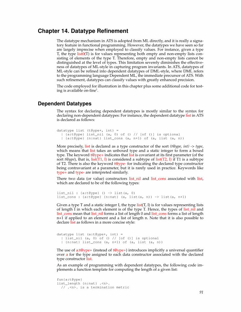
Chapter 14. Datatype Refinement
The datatype mechanism in ATS is adopted from ML directly, and it is really a signa-tory feature in functional programming. However, the datatypes we have seen so farare largely imprecise when employed to classify values. For instance, given a typeT, the type list0(T) is for values representing both empty and non-empty lists con-sisting of elements of the type T. Therefore, empty and non-empty lists cannot bedistinguished at the level of types. This limitation severely diminishes the effective-ness of datatypes of ML-style in capturing program invariants. In ATS, datatypes ofML-style can be refined into dependent datatypes of DML-style, where DML refersto the programming language Dependent ML, the immediate precursor of ATS. Withsuch refinement, datatypes can classify values with greatly enhanced precision.
The code employed for illustration in this chapter plus some additional code for test-ing is available on-line1.
Dependent DatatypesThe syntax for declaring dependent datatypes is mostly similar to the syntax fordeclaring non-dependent datatypes: For instance, the dependent datatype list in ATSis declared as follows:
datatype list (t@ype+, int) =| {a:t@ype} list_nil (a, 0) of () // [of ()] is optional| {a:t@ype} {n:nat} list_cons (a, n+1) of (a, list (a, n))
More precisely, list is declared as a type constructor of the sort (t@ype, int) -> type,which means that list takes an unboxed type and a static integer to form a boxedtype. The keyword t@ype+ indicates that list is covariant at its first parameter (of thesort t@ype), that is, list(T1, I) is considered a subtype of list(T2, I) if T1 is a subtypeof T2. There is also the keyword t@ype- for indicating the declared type constructorbeing contravariant at a parameter, but it is rarely used in practice. Keywords liketype+ and type- are interpreted similarly.
There two data (or value) constructors list_nil and list_cons associated with list,which are declared to be of the following types:
list_nil : {a:t@ype} () -> list(a, 0)list_cons : {a:t@ype} {n:nat} (a, list(a, n)) -> list(a, n+1)
Given a type T and a static integer I, the type list(T, I) is for values representing listsof length I in which each element is of the type T. Hence, the types of list_nil andlist_cons mean that list_nil forms a list of length 0 and list_cons forms a list of lengthn+1 if applied to an element and a list of length n. Note that it is also possible todeclare list as follows in a more concise style:
datatype list (a:t@ype+, int) =| list_nil (a, 0) of () // [of ()] is optional| {n:nat} list_cons (a, n+1) of (a, list (a, n))
The use of a:t@ype+ (instead of t@ype+) introduces implicitly a universal quantifierover a for the type assigned to each data constructor associated with the declaredtype constructor list.
As an example of programming with dependent datatypes, the following code im-plements a function template for computing the length of a given list:
fun{a:t@ype}list_length {n:nat} .<n>.// .<n>. is a termination metric
91
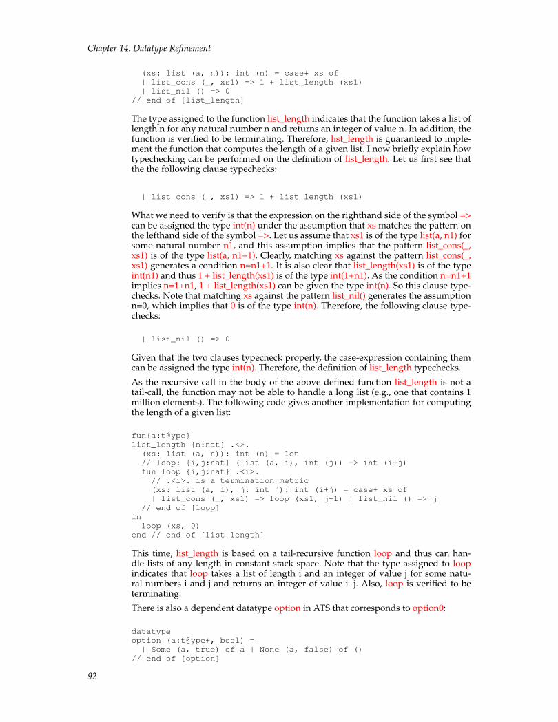
Chapter 14. Datatype Refinement
(xs: list (a, n)): int (n) = case+ xs of| list_cons (_, xs1) => 1 + list_length (xs1)| list_nil () => 0
// end of [list_length]
The type assigned to the function list_length indicates that the function takes a list oflength n for any natural number n and returns an integer of value n. In addition, thefunction is verified to be terminating. Therefore, list_length is guaranteed to imple-ment the function that computes the length of a given list. I now briefly explain howtypechecking can be performed on the definition of list_length. Let us first see thatthe the following clause typechecks:
| list_cons (_, xs1) => 1 + list_length (xs1)
What we need to verify is that the expression on the righthand side of the symbol =>can be assigned the type int(n) under the assumption that xs matches the pattern onthe lefthand side of the symbol =>. Let us assume that xs1 is of the type list(a, n1) forsome natural number n1, and this assumption implies that the pattern list_cons(_,xs1) is of the type list(a, n1+1). Clearly, matching xs against the pattern list_cons(_,xs1) generates a condition n=n1+1. It is also clear that list_length(xs1) is of the typeint(n1) and thus 1 + list_length(xs1) is of the type int(1+n1). As the condition n=n1+1implies n=1+n1, 1 + list_length(xs1) can be given the type int(n). So this clause type-checks. Note that matching xs against the pattern list_nil() generates the assumptionn=0, which implies that 0 is of the type int(n). Therefore, the following clause type-checks:
| list_nil () => 0
Given that the two clauses typecheck properly, the case-expression containing themcan be assigned the type int(n). Therefore, the definition of list_length typechecks.
As the recursive call in the body of the above defined function list_length is not atail-call, the function may not be able to handle a long list (e.g., one that contains 1million elements). The following code gives another implementation for computingthe length of a given list:
fun{a:t@ype}list_length {n:nat} .<>.(xs: list (a, n)): int (n) = let// loop: {i,j:nat} (list (a, i), int (j)) -> int (i+j)fun loop {i,j:nat} .<i>.// .<i>. is a termination metric(xs: list (a, i), j: int j): int (i+j) = case+ xs of| list_cons (_, xs1) => loop (xs1, j+1) | list_nil () => j
// end of [loop]inloop (xs, 0)
end // end of [list_length]
This time, list_length is based on a tail-recursive function loop and thus can han-dle lists of any length in constant stack space. Note that the type assigned to loopindicates that loop takes a list of length i and an integer of value j for some natu-ral numbers i and j and returns an integer of value i+j. Also, loop is verified to beterminating.
There is also a dependent datatype option in ATS that corresponds to option0:
datatypeoption (a:t@ype+, bool) =| Some (a, true) of a | None (a, false) of ()
// end of [option]
92
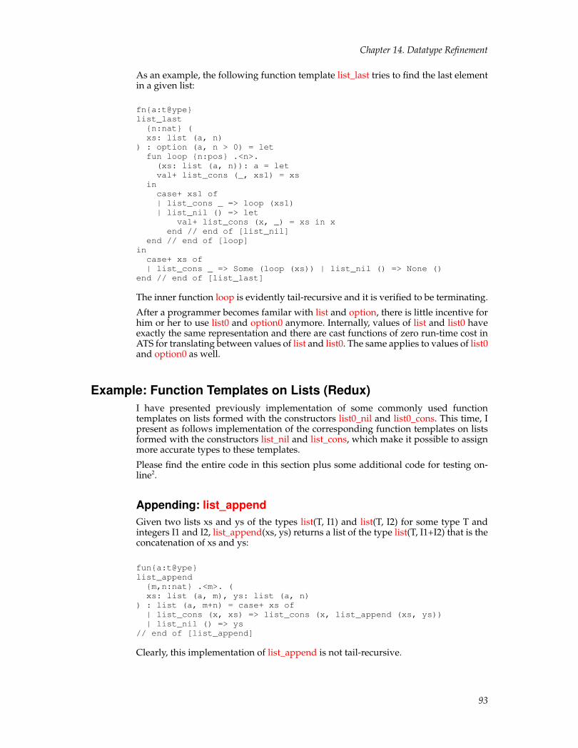
Chapter 14. Datatype Refinement
As an example, the following function template list_last tries to find the last elementin a given list:
fn{a:t@ype}list_last{n:nat} (xs: list (a, n)
) : option (a, n > 0) = letfun loop {n:pos} .<n>.(xs: list (a, n)): a = letval+ list_cons (_, xs1) = xs
incase+ xs1 of| list_cons _ => loop (xs1)| list_nil () => let
val+ list_cons (x, _) = xs in xend // end of [list_nil]
end // end of [loop]incase+ xs of| list_cons _ => Some (loop (xs)) | list_nil () => None ()
end // end of [list_last]
The inner function loop is evidently tail-recursive and it is verified to be terminating.
After a programmer becomes familar with list and option, there is little incentive forhim or her to use list0 and option0 anymore. Internally, values of list and list0 haveexactly the same representation and there are cast functions of zero run-time cost inATS for translating between values of list and list0. The same applies to values of list0and option0 as well.
Example: Function Templates on Lists (Redux)I have presented previously implementation of some commonly used functiontemplates on lists formed with the constructors list0_nil and list0_cons. This time, Ipresent as follows implementation of the corresponding function templates on listsformed with the constructors list_nil and list_cons, which make it possible to assignmore accurate types to these templates.
Please find the entire code in this section plus some additional code for testing on-line2.
Appending: list_appendGiven two lists xs and ys of the types list(T, I1) and list(T, I2) for some type T andintegers I1 and I2, list_append(xs, ys) returns a list of the type list(T, I1+I2) that is theconcatenation of xs and ys:
fun{a:t@ype}list_append{m,n:nat} .<m>. (xs: list (a, m), ys: list (a, n)
) : list (a, m+n) = case+ xs of| list_cons (x, xs) => list_cons (x, list_append (xs, ys))| list_nil () => ys
// end of [list_append]
Clearly, this implementation of list_append is not tail-recursive.
93

Chapter 14. Datatype Refinement
Reverse Appending: list_reverse_appendGiven two lists xs and ys of the type list(T, I1) and list(T, I2) for some type T andintegers I1 and I2, list_reverse_append(xs, ys) returns a list of the type list(T, I1+I2)that is the concatenation of the reverse of xs and ys:
fun{a:t@ype}list_reverse_append{m,n:nat} .<m>. (xs: list (a, m), ys: list (a, n)
) : list (a, m+n) = case+ xs of| list_cons (x, xs) =>
list_reverse_append (xs, list_cons (x, ys))| list_nil () => ys
// end of [list_reverse_append]
Clearly, this implementation of list_reverse_append is tail-recursive.
Reversing: list_reverseGiven a list xs, list_reverse(xs) returns the reverse of xs, which is of the same lengthas xs:
fun{a:t@ype}list_reverse {n:nat} .<>. // defined non-recursively(xs: list (a, n)): list (a, n) = list_reverse_append (xs, list_nil)
// end of [list_reverse]
Mapping: list_mapGiven a list xs of the type list(T1, I) for some type T1 and integer I and a closurefunction f of the type T1 -<cloref1> T2 for some T2, list_map(xs) returns a list ys ofthe type list(T2, I):
fun{a:t@ype}{b:t@ype}list_map {n:nat} .<n>. (xs: list (a, n), f: a -<cloref1> b
) : list (b, n) = case+ xs of| list_cons (x, xs) => list_cons (f x, list_map (xs, f))| list_nil () => list_nil ()
// end of [list_map]
Each element y in ys equals f(x), where x is the corresponding element in xs. Clearly,this implementation of list_map is not tail-recursive.
Zipping: list_zipGiven two lists xs and ys of the types list(T1, I) and list(T2, I) for some types T1 andT2 and integer I, respectively, list_zip(xs, ys) returns a list zs of the type list((T1, T2),I):
fun{a,b:t@ype}list_zip {n:nat} .<n>. (xs: list (a, n), ys: list (b, n)
) : list ((a, b), n) = case+ (xs, ys) of| (list_cons (x, xs),
94

Chapter 14. Datatype Refinement
list_cons (y, ys)) => list_cons ((x, y), list_zip (xs, ys))| (list_nil (), list_nil ()) => list_nil ()
// end of [list_zip]
Each element z in zs equals the pair (x, y), where x and y are the correspondingelements in xs and ys, respectively. Clearly, this implementation of list_zip is not tail-recursive.
Zipping with: list_zipwithGiven two lists xs and ys of the types list(T1, I) and list(T2, I) for some types T1 andT2 and integer I, respectively, and a closure function f of the type (T1, T2) -<cloref1>T3 for some type T3, list_zipwith(xs, ys, f) returns a list zs of the type list(T3, I):
fun{a,b:t@ype}{c:t@ype}list_zipwith{n:nat} .<n>. (xs: list (a, n)
, ys: list (b, n), f: (a, b) -<cloref1> c) : list (c, n) = case+ (xs, ys) of| (list_cons (x, xs), list_cons (y, ys)) =>
list_cons (f (x, y), list_zipwith (xs, ys, f))| (list_nil (), list_nil ()) => list_nil ()
// end of [list_zipwith]
Each element z in zs equals f(x, y), where x and y are the corresponding elements in xsand ys, respectively. Clearly, this implementation of list_zipwith is not tail-recursive.
Example: Mergesort on Lists (Redux)I have previously presented an implementation of mergesort on lists that are formedwith the constructors list0_nil and list0_cons. In this section, I give an implementa-tion of mergesort on lists formed with the constructors list_nil and list_cons. Thisimplementation is based on the same algorithm as the previous one but it assigns atype to the implemented sorting function that guarantees the function to be length-preserving, that is, the function always returns a list of the same length as the list itsorts.
The following defined function merge combines two ordered list (according to agiven ordering) into a single ordered list:
typedef lte (a:t@ype) = (a, a) -> bool
fun{a:t@ype}merge {m,n:nat} .<m+n>. (xs: list (a, m), ys: list (a, n), lte: lte a
) : list (a, m+n) =case+ xs of| list_cons (x, xs1) => (case+ ys of| list_cons (y, ys1) =>
if x \lte y thenlist_cons (x, merge (xs1, ys, lte))
elselist_cons (y, merge (xs, ys1, lte))
// end of [if]| list_nil () => xs) // end of [list_cons]
95

Chapter 14. Datatype Refinement
| list_nil () => ys// end of [merge]
Clearly, the type assigned to merge indicates that the function returns a list whoselength equals the sum of the lengths of the two input lists. Note that a terminationmetric is present for verifying that merge is a terminating function.
The following defined function mergesort mergesorts a list according to a given or-dering:
fun{a:t@ype}mergesort {n:nat} (xs: list (a, n), lte: lte a
) : list (a, n) = letfun msort {n:nat} .<n,n>. (xs: list (a, n), n: int n, lte: lte a
) : list (a, n) =if n >= 2 then split (xs, n, lte, n/2, list_nil) else xs
// end of [msort]and split{n:int | n >= 2} {i:nat | i <= n/2} .<n,i>. (xs: list (a, n-n/2+i)
, n: int n, lte: lte a, i: int i, xsf: list (a, n/2-i)) : list (a, n) =if i > 0 then letval+ list_cons (x, xs) = xs
insplit (xs, n, lte, i-1, list_cons (x, xsf))
end else letval xsf = list_reverse<a> (xsf) // make sorting stable!val xsf = list_of_list_vt (xsf) // linear list -> nonlinear listval xsf = msort (xsf, n/2, lte) and xs = msort (xs, n-n/2, lte)
inmerge (xsf, xs, lte)
end // end of [if]// end of [split]val n = list_length<a> (xs)
inmsort (xs, n, lte)
end // end of [mergesort]
The type assigned to mergesort indicates that mergesort returns a list of the samelength as its input list. The two inner functions msort and split are defined mutuallyrecursively, and the termination metrics for them are pairs of natural numbers thatare compared according to the standard lexicographic ordering on integer sequences.The type assigned to msort clearly indicates that its integer argument is required tobe the length of its list argument, and a mismatch between the two surely results in atype-error. The type assigned to split is particularly informative, depicting a relationbetween the arguments and the return value of the function that can be of great helpfor someone trying to understand the code. The function list_reverse returns a linearlist that is the reverse of its input, and the cast function list_of_list_vt turns a linearlist into a nonlinear one (while incuring no cost at run-time). I will explain what linearlists are elsewhere.
Please find the entire code in this section plus some additional code for testing on-line3.
Sequentiality of Pattern MatchingIn ATS, pattern matching is performed sequentially at run-time. In other words, aclause is selected only if a given value matches the pattern guard associated with thisclause but the value fails to match the pattern associated with any clause ahead of
96

Chapter 14. Datatype Refinement
it. Naturally, one may expect that the following implementation of list_zipwith alsotypechecks:
fun{a1,a2:t@ype}{b:t@ype}list_zipwith {n:nat} (xs1: list (a1, n)
, xs2: list (a2, n), f: (a1, a2) -<cloref1> b) : list (b, n) =case+ (xs1, xs2) of| (list_cons (x1, xs1), list_cons (x2, xs2)) =>
list_cons (f (x1, x2), list_zipwith (xs1, xs2, f))| (_, _) => list_nil ()
// end of [list_zipwith]
This, however, is not the case. In ATS, typechecking clauses is done nondeterministi-cally (rather than sequentially). In this example, the second clause fails to typecheckas it is done without the assumption that the given value pair (xs1, xs2) fails to matchthe pattern guard associated with the first clause. The second clause can be modifiedslightly as follows to pass typechecking:
| (_, _) =>> list_nil ()
The use of the symbol =>> (in place of =>) indicates to the typechecker that this clauseneeds to be typechecked under the sequentiality assumption that the given value thatmatches it does not match the pattern guards associated with any previous clauses.Therefore, when the modified second clause is typechecked, it can be assumed thatthe value pair (xs1, xs2) matching the pattern (_, _) must match one of the followingthree patterns:
• (list_cons (_, _), list_nil ())
• (list_nil (), list_cons (_, _))
• (list_nil (), list_nil ())
Given that xs1 and xs2 are of the same length, the typechecker can readily infer that(xs1, xs2) cannot match either of the first two patterns. After these two patterns areruled out, typechecking is essentially done as if the second clause was written asfollows:
| (list_nil (), list_nil ()) => list_nil ()
One may be wondering why typechecking clauses is not required to be done sequen-tially by default. The simple reason is that this requirement, if fully enforced, can havea great negative impact on the efficiency of typechecking. Therefore, it is a reasonabledesign to provide the programmer with an explict means to occasionally make useof the sequentiality assumption needed for typechecking a particular clause.
Example: Functional Random-Access ListsThe data structure I implement in this section is based on one presented in the booktitled Pure Funtional Data Structures by Chris Okasaki, where more elaboration ondata structures of this kind can be found.
Let us first declare a datatype as follows:
97

Chapter 14. Datatype Refinement
typedef pt (a:t@ype) = ’(a, a)
datatyperalist (a:t@ype+, n:int) =| RAnil (a, 0)| {n:pos} RAevn (a, 2*n) of ralist (pt a, n)| {n:nat} RAodd (a, 2*n+1) of (a, ralist (pt a, n))
// end of [ralist]
Given an unboxed type T and a static integer, the type ralist(T, I) is a boxed type forvalues representing lists of length I. The meaning of the three constructors RAnil,RAevn and RAodd can be briefly explained as follows:
• The constructor RAnil is for constructing a value representing the empty list.
• In order to construct a value representing a list of 2*I elements for some I > 0,we first construct a value representing a list of I pairs of adjacent elements in the(original) list and then apply the constructor RAevn to the value.
• In order to construct a value representing a list of 2*I+1 elements for some I >= 0,we take out the head of the list and construct a value representing a list of I pairsof adjacent elements in the tail of the (original) list and then apply the constructorRAodd to the head element and the value.
For example, the list of the first 5 positive integers is represented by the followingvalue:
RAodd(1, RAevn(RAodd( ’( ’(2, 3), ’(4, 5) ), RAnil())))
Values constructed by the constructors RAnil, RAevn and RAodd represent lists thatsupport operations of logrithmic time for accessing and updating list elements, andsuch lists are often referred to as random-access lists.
Note that the datatype ralist is not supported in ML even if the index representinglist length is erased. This kind of datatypes are often referred to as nested datatypes,which are also supported in Haskell.
The following defined function ralist_length computes the length of a random-accesslist:
fun{a:t@ype}ralist_length // O(log n){n:nat} .<n>.(xs: ralist (a, n)): int n =case+ xs of| RAnil () => 0| RAevn xxs => 2 * ralist_length<pt(a)> (xxs)| RAodd (_, xxs) => 2 * ralist_length<pt(a)> (xxs) + 1
// end of [ralist_length]
While the implementation of ralist_length is clearly not tail-recursive, this is hardlyof any practical concern as the time-complexity of ralist_length is O(log(n)).
Consing means to form a new list with an element and a list such that the element andthe list are the head and tail of the new list. The following defined function ralist_consimplements consing for random-access lists:
fun{a:t@ype}ralist_cons // O(1), amortized{n:nat} .<n>.(x0: a, xs: ralist (a, n)): ralist (a, n+1) =case+ xs of| RAnil () => RAodd (x0, RAnil)
98

Chapter 14. Datatype Refinement
| RAevn (xxs) => RAodd (x0, xxs)| RAodd (x1, xxs) =>
RAevn (ralist_cons<pt(a)> ( ’(x0, x1), xxs ))// end of [RAodd]
// end of [ralist_cons]
In the worst case (where the length of xs is a power of 2 minus 1), ralist_constakes O(log(n))-time to finish. However, it can be proven that the amortizedtime-complexity of consing on random-access lists is O(1).
Unconsing does the opposite of consing: It returns a pair consisting of the head andtail of a given non-empty list. The following defined function ralist_uncons imple-ments unconsing for random-access lists:
fun{a:t@ype}ralist_uncons // O(1), amortized{n:pos} .<n>.(xs: ralist (a, n)): (a, ralist (a, n-1)) =case+ xs of| RAevn (xxs) => let
val (xx, xxs) = ralist_uncons<pt(a)> (xxs)in(xx.0, RAodd (xx.1, xxs))
end // end of [RAevn]| RAodd (x, xxs) => (case+ xxs of
(*// Note: [=>>] is needed for enforcing sequentiality// during typechecking:*)
RAnil () => (x, RAnil) | _ =>> (x, RAevn (xxs))) // end of [RAodd]
// end of [ralist_uncons]
Like ralist_cons, ralist_uncons takes O(log(n))-time to finish when the length of xsis a power of 2. However, its amortized time-complexity is also O(1). It is highlyprobable for a programmer to implement the second matching clause in the body ofralist_uncons as follows:
| RAodd (x, xxs) => (x, RAevn (xxs))
For instance, I myself did this. This is a program error as the invariant can potentiallybe broken that states RAevn being only applied to a value representing a non-emptylist. The error is readily caught by the typechecker of ATS but it is most likely togo unnoticed in a setting where the invariant on the constructor RAevn can not becaptured at compile-time.
Given a random-access list xs of length n, the elements in it are numbered from 0 ton-1, inclusively. We can find element i in the list xs, where i is assumed to be a naturalnumber less than n, by implementing the following algorithm:
• Assume the length n is even. Then xs is of the form RAevn(xxs), where xxs is a listof pairs. Let i2 be i/2 and we find element i2 in xxs, which is a pair. Let xx refer tothis pair. If i is even, then the left component of xx is element i in xs. Otherwise, theright component is.
• Assume the length n is odd. Then xs is of the form RAodd(x, xxs), where xxs is a listof pairs. If i equals 0, the x is element i in xs. Otherwise, let i1 be i-1 and i2 be i1/2and we find element i2 in xxs, which is a pair. Let xx refer to this pair. If i1 is even,then the left component of xx is element i in xs. Otherwise, the right component is.
The following function ralist_lookup is implemented precisely according to the givenalgorithm:
99
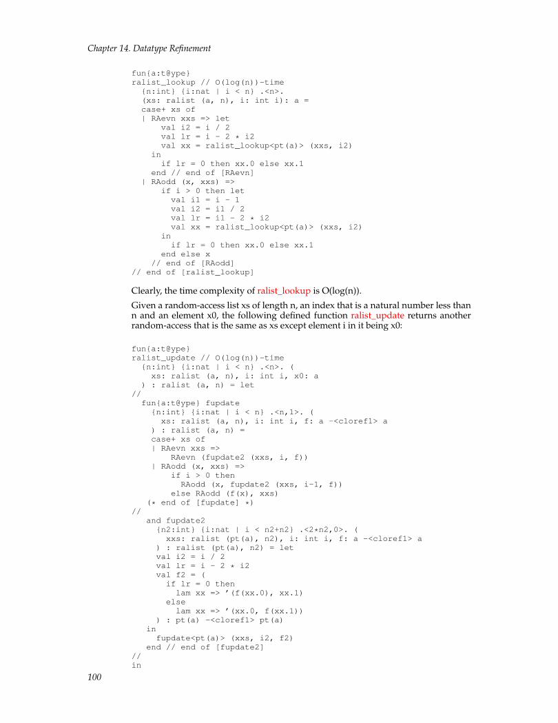
Chapter 14. Datatype Refinement
fun{a:t@ype}ralist_lookup // O(log(n))-time{n:int} {i:nat | i < n} .<n>.(xs: ralist (a, n), i: int i): a =case+ xs of| RAevn xxs => let
val i2 = i / 2val lr = i - 2 * i2val xx = ralist_lookup<pt(a)> (xxs, i2)
inif lr = 0 then xx.0 else xx.1
end // end of [RAevn]| RAodd (x, xxs) =>
if i > 0 then letval i1 = i - 1val i2 = i1 / 2val lr = i1 - 2 * i2val xx = ralist_lookup<pt(a)> (xxs, i2)
inif lr = 0 then xx.0 else xx.1
end else x// end of [RAodd]
// end of [ralist_lookup]
Clearly, the time complexity of ralist_lookup is O(log(n)).
Given a random-access list xs of length n, an index that is a natural number less thann and an element x0, the following defined function ralist_update returns anotherrandom-access that is the same as xs except element i in it being x0:
fun{a:t@ype}ralist_update // O(log(n))-time{n:int} {i:nat | i < n} .<n>. (xs: ralist (a, n), i: int i, x0: a
) : ralist (a, n) = let//fun{a:t@ype} fupdate{n:int} {i:nat | i < n} .<n,1>. (xs: ralist (a, n), i: int i, f: a -<cloref1> a
) : ralist (a, n) =case+ xs of| RAevn xxs =>
RAevn (fupdate2 (xxs, i, f))| RAodd (x, xxs) =>
if i > 0 thenRAodd (x, fupdate2 (xxs, i-1, f))
else RAodd (f(x), xxs)(* end of [fupdate] *)
//and fupdate2{n2:int} {i:nat | i < n2+n2} .<2*n2,0>. (
xxs: ralist (pt(a), n2), i: int i, f: a -<cloref1> a) : ralist (pt(a), n2) = letval i2 = i / 2val lr = i - 2 * i2val f2 = (if lr = 0 thenlam xx => ’(f(xx.0), xx.1)
elselam xx => ’(xx.0, f(xx.1))
) : pt(a) -<cloref1> pt(a)infupdate<pt(a)> (xxs, i2, f2)
end // end of [fupdate2]//in
100
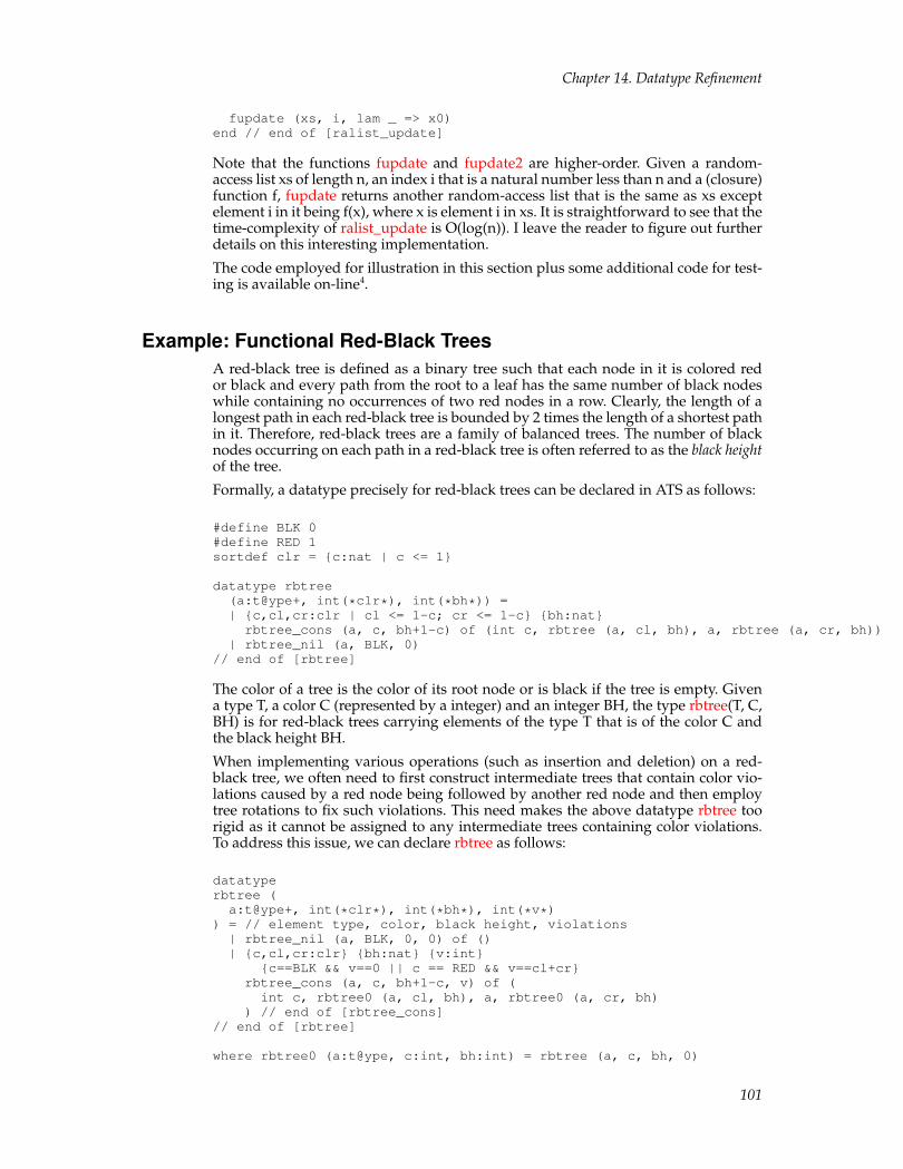
Chapter 14. Datatype Refinement
fupdate (xs, i, lam _ => x0)end // end of [ralist_update]
Note that the functions fupdate and fupdate2 are higher-order. Given a random-access list xs of length n, an index i that is a natural number less than n and a (closure)function f, fupdate returns another random-access list that is the same as xs exceptelement i in it being f(x), where x is element i in xs. It is straightforward to see that thetime-complexity of ralist_update is O(log(n)). I leave the reader to figure out furtherdetails on this interesting implementation.
The code employed for illustration in this section plus some additional code for test-ing is available on-line4.
Example: Functional Red-Black TreesA red-black tree is defined as a binary tree such that each node in it is colored redor black and every path from the root to a leaf has the same number of black nodeswhile containing no occurrences of two red nodes in a row. Clearly, the length of alongest path in each red-black tree is bounded by 2 times the length of a shortest pathin it. Therefore, red-black trees are a family of balanced trees. The number of blacknodes occurring on each path in a red-black tree is often referred to as the black heightof the tree.
Formally, a datatype precisely for red-black trees can be declared in ATS as follows:
#define BLK 0#define RED 1sortdef clr = {c:nat | c <= 1}
datatype rbtree(a:t@ype+, int(*clr*), int(*bh*)) =| {c,cl,cr:clr | cl <= 1-c; cr <= 1-c} {bh:nat}rbtree_cons (a, c, bh+1-c) of (int c, rbtree (a, cl, bh), a, rbtree (a, cr, bh))
| rbtree_nil (a, BLK, 0)// end of [rbtree]
The color of a tree is the color of its root node or is black if the tree is empty. Givena type T, a color C (represented by a integer) and an integer BH, the type rbtree(T, C,BH) is for red-black trees carrying elements of the type T that is of the color C andthe black height BH.
When implementing various operations (such as insertion and deletion) on a red-black tree, we often need to first construct intermediate trees that contain color vio-lations caused by a red node being followed by another red node and then employtree rotations to fix such violations. This need makes the above datatype rbtree toorigid as it cannot be assigned to any intermediate trees containing color violations.To address this issue, we can declare rbtree as follows:
datatyperbtree (a:t@ype+, int(*clr*), int(*bh*), int(*v*)
) = // element type, color, black height, violations| rbtree_nil (a, BLK, 0, 0) of ()| {c,cl,cr:clr} {bh:nat} {v:int}
{c==BLK && v==0 || c == RED && v==cl+cr}rbtree_cons (a, c, bh+1-c, v) of (int c, rbtree0 (a, cl, bh), a, rbtree0 (a, cr, bh)
) // end of [rbtree_cons]// end of [rbtree]
where rbtree0 (a:t@ype, c:int, bh:int) = rbtree (a, c, bh, 0)
101

Chapter 14. Datatype Refinement
We count each occurrence of two red nodes in a row as one color violation. Given atype T, a color C (represented by a integer), an integer BH and an integer V, the typerbtree(T, C, BH, V) is for trees carrying elements of the type T that is of the color Cand the black height BH and contains exactly V color violations. Therefore, the typerbtree(T, C, BH, 0) is for valid red-black trees (containing no color violations).
Given a tree containing at most one color violation, an element and another tree con-taining no violations, the following operation constructs a valid red-black tree:
fn{a:t@ype}insfix_l // right rotation for fixing left insertion{cl,cr:clr} {bh:nat} {v:nat} (tl: rbtree (a, cl, bh, v), x0: a, tr: rbtree (a, cr, bh, 0)
) : [c:clr] rbtree0 (a, c, bh+1) = let#define B BLK; #define R RED; #define cons rbtree_cons
incase+ (tl, x0, tr) of| (cons (R, cons (R, a, x, b), y, c), z, d) =>
cons (R, cons (B, a, x, b), y, cons (B, c, z, d)) // shallow rot| (cons (R, a, x, cons (R, b, y, c)), z, d) =>
cons (R, cons (B, a, x, b), y, cons (B, c, z, d)) // deep rotation| (a, x, b) =>> cons (B, a, x, b)
end // end of [insfix_l]
By simply reading the interface of insfix_l, we can see that the two tree argumentsare required to be of the same black height bh for some natural number bh and thereturned tree is of the black height bh+1.
The following operation insfix_r is just the mirror image of insfix_l:
fn{a:t@ype}insfix_r // left rotation for fixing right insertion{cl,cr:clr} {bh:nat} {v:nat} (tl: rbtree (a, cl, bh, 0), x0: a, tr: rbtree (a, cr, bh, v)
) : [c:clr] rbtree0 (a, c, bh+1) = let#define B BLK; #define R RED; #define cons rbtree_cons
incase+ (tl, x0, tr) of| (a, x, cons (R, b, y, cons (R, c, z, d))) =>
cons (R, cons (B, a, x, b), y, cons (B, c, z, d)) // shallow rot| (a, x, cons (R, cons (R, b, y, c), z, d)) =>
cons (R, cons (B, a, x, b), y, cons (B, c, z, d)) // deep rotation| (a, x, b) =>> cons (B, a, x, b)
end // end of [insfix_r]
The preparation for implementing insertion on a red-black tree is all done by now,and we are ready to see an implementation of insertion guaranteeing that the treeobtained from inserting an element into a given red-black tree is always a valid red-black tree itself. This guarantee is precisely captured in the following interface forinsertion:
externfun{a:t@ype}rbtree_insert{c:clr} {bh:nat} (t: rbtree0 (a, c, bh), x0: a, cmp: cmp a
) : [bh1:nat] rbtree0 (a, BLK, bh1)
Interestingly, this interface also implies that the tree returned by a call to rbtree_insertis always black. The code presented below gives an implementation of rbtree_insert:
implement{a}rbtree_insert
102
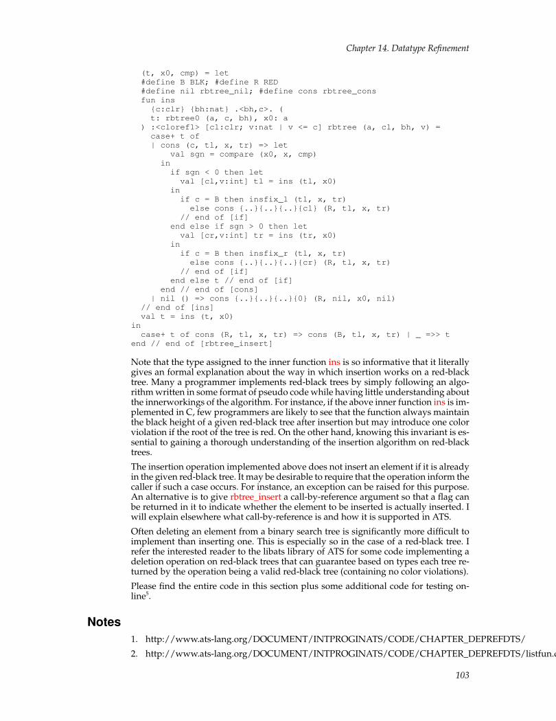
Chapter 14. Datatype Refinement
(t, x0, cmp) = let#define B BLK; #define R RED#define nil rbtree_nil; #define cons rbtree_consfun ins{c:clr} {bh:nat} .<bh,c>. (t: rbtree0 (a, c, bh), x0: a
) :<cloref1> [cl:clr; v:nat | v <= c] rbtree (a, cl, bh, v) =case+ t of| cons (c, tl, x, tr) => let
val sgn = compare (x0, x, cmp)inif sgn < 0 then letval [cl,v:int] tl = ins (tl, x0)
inif c = B then insfix_l (tl, x, tr)else cons {..}{..}{..}{cl} (R, tl, x, tr)
// end of [if]end else if sgn > 0 then letval [cr,v:int] tr = ins (tr, x0)
inif c = B then insfix_r (tl, x, tr)else cons {..}{..}{..}{cr} (R, tl, x, tr)
// end of [if]end else t // end of [if]
end // end of [cons]| nil () => cons {..}{..}{..}{0} (R, nil, x0, nil)
// end of [ins]val t = ins (t, x0)
incase+ t of cons (R, tl, x, tr) => cons (B, tl, x, tr) | _ =>> t
end // end of [rbtree_insert]
Note that the type assigned to the inner function ins is so informative that it literallygives an formal explanation about the way in which insertion works on a red-blacktree. Many a programmer implements red-black trees by simply following an algo-rithm written in some format of pseudo code while having little understanding aboutthe innerworkings of the algorithm. For instance, if the above inner function ins is im-plemented in C, few programmers are likely to see that the function always maintainthe black height of a given red-black tree after insertion but may introduce one colorviolation if the root of the tree is red. On the other hand, knowing this invariant is es-sential to gaining a thorough understanding of the insertion algorithm on red-blacktrees.
The insertion operation implemented above does not insert an element if it is alreadyin the given red-black tree. It may be desirable to require that the operation inform thecaller if such a case occurs. For instance, an exception can be raised for this purpose.An alternative is to give rbtree_insert a call-by-reference argument so that a flag canbe returned in it to indicate whether the element to be inserted is actually inserted. Iwill explain elsewhere what call-by-reference is and how it is supported in ATS.
Often deleting an element from a binary search tree is significantly more difficult toimplement than inserting one. This is especially so in the case of a red-black tree. Irefer the interested reader to the libats library of ATS for some code implementing adeletion operation on red-black trees that can guarantee based on types each tree re-turned by the operation being a valid red-black tree (containing no color violations).
Please find the entire code in this section plus some additional code for testing on-line5.
Notes1. http://www.ats-lang.org/DOCUMENT/INTPROGINATS/CODE/CHAPTER_DEPREFDTS/
2. http://www.ats-lang.org/DOCUMENT/INTPROGINATS/CODE/CHAPTER_DEPREFDTS/listfun.dats
103

Chapter 14. Datatype Refinement
3. http://www.ats-lang.org/DOCUMENT/INTPROGINATS/CODE/CHAPTER_DEPREFDTS/mergesort.dats
4. http://www.ats-lang.org/DOCUMENT/INTPROGINATS/CODE/CHAPTER_DEPREFDTS/ralist.dats
5. http://www.ats-lang.org/DOCUMENT/INTPROGINATS/CODE/CHAPTER_DEPREFDTS/rbtree.dats
104

Chapter 15. Theorem-Proving in ATS/LF
Within the ATS programming langauge system, there is a component named ATS/LFfor supporting (interactive) therorem-proving. In ATS/LF, theorem-proving is doneby constructing proofs as total functional programs. It will soon become clear that thisstyle of theorem-proving can be combined cohesively with functional programmingto yield a programming paradigm that is considered the signature of ATS: program-ming with theorem-proving. Moreover, ATS/LF can be employed to encode variousdeduction systems and their meta-properties.
Please find on-line1 the code employed for illustration in this chapter plus some ad-ditional code for testing.
Encoding Relations as DatapropsIn the statics of ATS, there is a built-in sort prop for static terms that represent typesfor proofs. A static term of the sort prop can also be referred to as a type or moreaccurately, a prop-type or just a prop. A dataprop can be declared in a manner that ismostly similar to the declaration of a datatype. For instance, a prop construct FIB isintroduced in the following dataprop declaration:
dataprop FIB (int, int) =| FIB0 (0, 0) of () // [of ()] can be dropped| FIB1 (1, 1) of () // [of ()] can be dropped| {n:nat} {r0,r1:nat}FIB2 (n+2, r0+r1) of (FIB (n, r0), FIB (n+1, r1))
// end of [FIB]
The sort assigned to FIB is (int, int) -> prop, indicating that FIB takes two static inte-gers to form a prop-type. There are three data (or proof) constructors associated withFIB: FIB0, FIB1 and FIB2, which are assigned the following function types (or moreaccurately, prop-types):
• FIB0: () -> FIB (0, 0)
• FIB1: () -> FIB (1, 1)
• FIB2: {n:nat} {r0,r1:int} (FIB(n, r0), FIB(n+1, r1)) -> FIB(n+2, r0+r1)
Given a natural number n and an integer r, it should be clear that FIB(n, r) encodesthe relation fib(n) = r, where fib is defined by the following three equations:
• fib(0) = 0, and
• fib(1) = 1, and
• fib(n+2) = fib(n+1) + fib(n) for n >= 2.
A proof value of the prop FIB(n, r) can be constructed if and only if fib(n) equals r. Forinstance, the proof value FIB2(FIB0(), FIB1()) is assigned the prop FIB(2, 1), attestingto fib(2) equaling 1.
As another example of dataprop, the following declaration introduces a prop con-structor MUL together with three associated proof constructors:
dataprop MUL (int, int, int) =| {n:int} MULbas (0, n, 0) of ()| {m:nat} {n:int} {p:int}MULind (m+1, n, p+n) of MUL (m, n, p)
| {m:pos} {n:int} {p:int}MULneg (~m, n, ~p) of MUL (m, n, p)
105

Chapter 15. Theorem-Proving in ATS/LF
// end of [MUL]
Given three integers m, n and p, the prop MUL(m, n, p) encodes the relation m*n= p. As for MULbas, MULind and MULneg, they correspond to the following threeequations, respectively:
• 0*n = 0 for every integer n, and
• (m+1)*n = m*n + n for each pair of integers m and n, and
• (~m)*n = ~(m*n) for each pair of integers m and n.
In other words, the dataprop declaration for MUL encodes the relation that repre-sents the standard multiplication function on integers.
It can be readily noticed that the process of encoding a functional relation (i.e., a rela-tion representing a function) as a dataprop is analogous to implementing a functionin a logic programming language such as Prolog.
Constructing Proofs as Total FunctionsTheorems are represented as types (or more accurately, props) in ATS/LF. For in-stance, the following prop states that integer multiplication is commutative:
{m,n:int} {p:int} MUL (m, n, p) -<prf> MUL (n, m, p)
Constructing a proof for a theorem in ATS/LF means implementing a total value(which is most likely to be a total function) of the type that is the encoding of thetheorem in ATS/LF, where being total means being pure and terminating. Pleasenote that this style of theorem-proving may seem rather peculiar to those who havenever tried it before.
As a simple introductory example, let us first construct a proof function in ATS/LFthat is given the following interface:
prfun mut_istot {m,n:int} (): [p:int] MUL (m, n, p)
The keyword prfun indicates that the interface is for a proof function (in contrast toa non-proof function). Note that mul_istot is declared to be of the following type (ormore accurately, prop):
{m,n:int} () -<prf> [p:int] MUL (m, n, p)
which essentially states that integer multiplication is a total function: Given any twointegers m and n, there exists an integer p such that m, n and p are related accordingto the structurally inductively defined relation MUL. The following code gives animplementation of mul_istot:
implementmul_istot {m,n} () = letprfun istot{m:nat;n:int} .<m>. (): [p:int] MUL (m, n, p) =sif m > 0 then MULind (istot {m-1,n} ()) else MULbas ()
// end of [istot]insif m >= 0 then istot {m,n} () else MULneg (istot {~m,n} ())
end // end of [mul_istot]
106
Chapter 15. Theorem-Proving in ATS/LF
Note that the inner proof function istot encodes a proof showing that there existsan integer p for any given natural number m and integer n such that m, n and pare related (according to MUL). The keyword sif is used for forming a conditional(proof) expression in which the test is a static expression. The proof encoded by istotproceeds by induction on m; if m > 0 holds, then there exists an integer p1 such thatm-1, n and p1 are related by induction hypothesis (on m-1) and thus m, n and p arerelated for p = p1+n according to the rule encoded by MULind; if m = 0, then m, nand p are related for p = 0. The proof encoded by the implementation of mul_istotgoes like this: if m is a natural number, then the lemma proven by istot shows thatm, n and some p are related; if m is negative, then the same lemma shows that ~m,n and p1 are related for some integer p1 and thus m, n and p are related for p = ~p1according to the rule encoded by MULneg.
As another example of theorem-proving in ATS/LF, a proof function of the namemul_isfun is given as follows:
prfn mul_isfun{m,n:int} {p1,p2:int} (pf1: MUL (m, n, p1), pf2: MUL (m, n, p2)
) : [p1==p2] void = letprfun isfun{m:nat;n:int} {p1,p2:int} .<m>. (pf1: MUL (m, n, p1), pf2: MUL (m, n, p2)
) : [p1==p2] void =case+ pf1 of| MULind (pf1prev) => let
prval MULind (pf2prev) = pf2 in isfun (pf1prev, pf2prev)end // end of [MULind]
| MULbas () => letprval MULbas () = pf2 in ()
end // end of [MULbas]// end of [isfun]
incase+ pf1 of| MULneg (pf1nat) => let
prval MULneg (pf2nat) = pf2 in isfun (pf1nat, pf2nat)end // end of [MULneg]
| _ =>> isfun (pf1, pf2)end // end of [mul_isfun]
The keyword prfn is used for defining a non-recursive proof function, and the key-word prval for introducing bindings that relate names to proof expressions, that is,expressions of prop-types. As far as pattern matching exhaustiveness is concerned,prval is equivalent to val+ (as proofs cannot contain any effects such as failures ofpattern matching).
What mul_isfun proves is that the relation MUL is functional on its first two argu-ments: If m, n and p1 are related according to MUL and m, n and p2 are also relatedaccording to MUL, then p1 and p2 are equal. The statement is first proven by the in-ner proof function isfun under the assumption that m is a natural number, and thenthe assumption is dropped. Let us now take a look at the first matching clause in thebody of isfun. If the clause is chosen, then pf1 matches the pattern MULind(pf1prev)and thus pf1prev is of the type MUL(m1, n1, q1) for some natural number m1 and in-teger n1 and integer p1 such that m=m1+1, n=n1, and p1=q1+n1. This means that pf2must be of the form MULind(pf2prev) for some pf2prev of the type MUL(m2, n2, q2)such that m2+1=m, n2=n and p2=q2+n2. By calling isfun on pf1prev and pf2prev,which amounts to invoking the induction hypothesis on m-1, we establish q1=q2,which implies p1=p2. The second matching clause in the body of isfun can be readilyunderstood, which corresponds to the base case in the inductive proof encoded byisfun.
107
Chapter 15. Theorem-Proving in ATS/LF
Example: Proving Distributivity of MultiplicationThe distributivity of multiplication over addition means that the following equationholds
m * (n1 + n2) = m * n1 + m * n2
for m, n1 and n2 ranging over integers. Clearly, a direct encoding of the equation isgiven by the following (proof) function interface:
externprfun mul_distribute {m:int} {n1,n2:int} {p1,p2:int}(pf1: MUL (m, n1, p1), pf2: MUL (m, n2, p2)): MUL (m, n1+n2, p1+p2)
// end of [mul_distribute]
Plainly speaking, the encoding states that the product of m and (n1+n2) is p1+p2 ifthe product of m and n1 is p1 and the product of m and n2 is p2. An implementationof mul_distribute is given as follows:
implementmul_distribute{m} {n1,n2} {p1,p2} (pf1, pf2) = letprfun aux{m:nat}{n1,n2:int}{p1,p2:int}.<m>. (pf1: MUL (m, n1, p1), pf2: MUL (m, n2, p2)
) : MUL (m, n1+n2, p1+p2) =case+ (pf1, pf2) of| (MULbas (), MULbas ()) => MULbas ()| (MULind pf1, MULind pf2) => MULind (aux (pf1, pf2))
// end of [aux]insif m >= 0 thenaux (pf1, pf2)
else letprval MULneg (pf1) = pf1prval MULneg (pf2) = pf2
inMULneg (aux (pf1, pf2))
endend // end of [mul_distribute]
In essence, the inner function aux encodes a straighforward proof based on mathe-matical induction that establishes the following equation:
m * (n1 + n2) = m * n1 + m * n2
for m ranging over natural numbers and n1 and n2 ranging over integers. The func-tion mul_distribute can then be implemented immediately based on aux.
DatasortsA datasort is rather similar to a dataype. However, the former is declared in the staticsof ATS while the latter in the dynamics of ATS. To see a typical need for datasorts, letus try to encode a theorem in ATS stating that s is strictly less than 2h if s and h are
108

Chapter 15. Theorem-Proving in ATS/LF
the size and height, respectively, of a given binary tree. To represent binary trees inthe statics, we first declare a datasort as follows:
datasort tree = E of () | B of (tree, tree)
The name of the declared datasort is tree and there are two constructor associatedwith it: E and B, where E forms the empty tree and B forms a tree by joining twogiven trees. For instance, B(E(), E()) is a static term of the sort tree that represents asingleton tree, that is, a tree consisting of exactly one node. Please note that the treesformed by E and B are really just tree skeletons carrying no data.
We now declare two dataprops as follows for capturing the notion of size and heightof trees:
dataprop SZ (tree, int) =| SZE (E (), 0) of ()| {tl,tr:tree} {sl,sr:nat}SZB (B (tl, tr), 1+sl+sr) of (SZ (tl, sl), SZ (tr, sr))
// end of [SZ]
dataprop HT (tree, int) =| HTE (E (), 0) of ()| {tl,tr:tree} {hl,hr:nat}HTB (B (tl, tr), 1+max(hl,hr)) of (HT (tl, hl), HT (tr, hr))
// end of [HT]
Given a tree t and an integer s, SZ(t, s) encodes the relation that the size of t equals s.Similiarly, given a tree t and an integer h, HZ(t, h) encodes the relation that the heightof t equals h.
As the power function (of base 2) is not available in the statics of ATS, we declare adataprop as follows to capture it:
dataprop POW2 (int, int) =| POW2bas (0, 1)| {n:nat} {p:int} POW2ind (n+1, p+p) of POW2 (n, p)
// end of [POW2]
Given two integers h and p, POW2 (h, p) encodes the relation that 2h equals p.
It should be clear by now that the following proof function interface encodes thetheorem stating that s is strictly less than 2h if s and h are the size and height of agiven binary tree:
externprfun lemma_tree_size_height{t:tree} {s,h:nat} {p:int} (pf1: SZ (t, s), pf2: HT (t, h), pf3: POW2 (h, p)
) : [s < p] void // end of [prfun]
Let us now construct an implementation of this proof function as follows.
We first establish some elementary properties on the power function (of base 2):
prfun pow2_istot{h:nat} .<h>. (): [p:int] POW2 (h, p) =sif h > 0 then POW2ind (pow2_istot {h-1} ()) else POW2bas ()
// end of [pow2_istot]
prfun pow2_pos{h:nat} {p:int} .<h>.(pf: POW2 (h, p)): [p > 0] void =case+ pf of
109

Chapter 15. Theorem-Proving in ATS/LF
| POW2ind (pf1) => pow2_pos (pf1) | POW2bas () => ()// end of [pow2_pos]
prfun pow2_inc{h1,h2:nat | h1 <= h2} {p1,p2:int} .<h2>.(pf1: POW2 (h1, p1), pf2: POW2 (h2, p2)): [p1 <= p2] void =case+ pf1 of| POW2ind (pf11) => let
prval POW2ind (pf21) = pf2 in pow2_inc (pf11, pf21)end
| POW2bas () => pow2_pos (pf2)// end of [pow2_inc]
Clearly, pow2_istot shows that the relation encoded by the dataprop POW2 is a to-tal relation; pow2_pos proves that the power of each natural number is positive;pow2_inc establishes that the power function is increasing.
The function lemma_tree_size_height can be implemented as follows:
implementlemma_tree_size_height(pf1, pf2, pf3) = let
//prfun lemma{t:tree} {s,h:nat} {p:int} .<t>. (pf1: SZ (t, s), pf2: HT (t, h), pf3: POW2 (h, p)
) : [p > s] void =scase t of| B (tl, tr) => let
prval SZB (pf1l, pf1r) = pf1prval HTB {tl,tr} {hl,hr} (pf2l, pf2r) = pf2prval POW2ind (pf31) = pf3prval pf3l = pow2_istot {hl} ()prval pf3r = pow2_istot {hr} ()prval () = lemma (pf1l, pf2l, pf3l)prval () = lemma (pf1r, pf2r, pf3r)prval () = pow2_inc (pf3l, pf31)prval () = pow2_inc (pf3r, pf31)
in// nothing
end // end of [B]| E () => let
prval SZE () = pf1prval HTE () = pf2prval POW2bas () = pf3
in// nothing
end // end of [E]//inlemma (pf1, pf2, pf3)
end // end of [lemma_tree_size_height]
The inner function lemma, which is given a termination metric consisting of a staticterm of the sort tree, corresponds to a proof based on structural induction (wherethe involved structure is the binary tree t). Given two terms t1 and t2 of the sorttree, t1 is (strictly) less than t2 if t1 is a (proper) substructure of t2. Evidently, this isa well-founded ordering. The keyword scase is used to form a dynamic expressionthat does case-analysis on a static term (built by constructors associated with somedeclared datasort). So the relation between sif and scase is essentially parallel to thatbetween if and case. Please find the entirety of the above code on-line2.
110
Chapter 15. Theorem-Proving in ATS/LF
Example: Proving Properties on Braun TreesAs stated previously in this book, a binary tree is a Braun tree if it is empty or if itsleft and right subtrees are Braun trees and the size of the left one minus the size of theright one is either 0 or 1. Formally, we can declare the following dataprop isBraun tocapture the notion of Braun trees:
dataprop isBraun (tree) =| isBraunE (E) of ()| {tl,tr:tree}{sl,sr:nat | sr <= sl; sl <= sr + 1}isBraunB (B(tl, tr)) of (isBraun tl, isBraun tr, SZ (tl, sl), SZ (tr, sr)
) // end of [isBraunB]// end of [isBraun]
We first prove that there exists a Braun tree of any given size. This property can beencoded as follows in ATS:
externprfun lemma_existence {n:nat} (): [t:tree] (isBraun (t), SZ (t, n))
Literally, the type assigned to lemma_existence means that there exists a tree t for anygiven natural number n such that t is a Braun tree and the size of t is n. The followingcode gives an implementation of lemma_existence:
implementlemma_existence {n} () = letprfun lemma {n:nat} .<n>.(): [t:tree] (isBraun (t), SZ (t, n)) =sif n > 0 then letstadef nl = n / 2 // size for the left subtreestadef nr = n - 1 - nl // size for the right subtreeval (pfl1, pfl2) = lemma {nl} ()and (pfr1, pfr2) = lemma {nr} ()
in(isBraunB (pfl1, pfr1, pfl2, pfr2), SZB (pfl2, pfr2))
end else(isBraunE (), SZE ())
// end of [sif]inlemma {n} ()
end // end of [lemma_existence]
Note that stadef is a keyword in ATS for introducting a static binding between a nameand a static term (of any sort). If one prefers, this keyword can be chosen to replacethe keyword typedef (for introducing a name and a static term of the sort t@ype).
Next we show that two Braun trees of the same size are identical. This property canbe encoded as follows:
externprfun lemma_unicity {n:nat} {t1,t2:tree} (pf1: isBraun t1, pf2: isBraun t2, pf3: SZ (t1, n), pf4: SZ (t2, n)
) : EQ (t1, t2) // end of [lemma_unicity]
where EQ is a prop-constructor introduced by the following dataprop declaration:
dataprop EQ (tree, tree) =| EQE (E, E) of ()
111

Chapter 15. Theorem-Proving in ATS/LF
| {t1l,t1r:tree} {t2l,t2r:tree}EQB (B (t1l, t1r), B (t2l, t2r)) of (EQ (t1l, t2l), EQ (t1r, t2r))
// end of [EQ]
Clearly, EQ is the inductively defined equality on trees. An implementation of theproof function lemma_unicity is presented as follows:
implementlemma_unicity (pf1, pf2, pf3, pf4) = letprfun lemma {n:nat} {t1,t2:tree} .<n>. (pf1: isBraun t1, pf2: isBraun t2, pf3: SZ (t1, n), pf4: SZ (t2, n)
) : EQ (t1, t2) =sif n > 0 then letprval SZB (pf3l, pf3r) = pf3prval SZB (pf4l, pf4r) = pf4prval isBraunB (pf1l, pf1r, pf1lsz, pf1rsz) = pf1prval isBraunB (pf2l, pf2r, pf2lsz, pf2rsz) = pf2prval () = SZ_istot (pf1lsz, pf3l) and () = SZ_istot (pf1rsz, pf3r)prval () = SZ_istot (pf2lsz, pf4l) and () = SZ_istot (pf2rsz, pf4r)prval pfeql = lemma (pf1l, pf2l, pf3l, pf4l)prval pfeqr = lemma (pf1r, pf2r, pf3r, pf4r)
inEQB (pfeql, pfeqr)
end else letprval SZE () = pf3 and SZE () = pf4prval isBraunE () = pf1 and isBraunE () = pf2
inEQE ()
end // end of [sif]inlemma (pf1, pf2, pf3, pf4)
end // end of [lemma_unicity]
Note that the proof function SZ_istot in this implementation of lemma_unicity isgiven the following interface:
externprfun SZ_istot {t:tree} {n1,n2:int}(pf1: SZ (t, n1), pf2: SZ (t, n2)): [n1==n2] void
which simply states that SZ is a functional relation with respect to its first parameter,that is, there is at most one n for every given t such that t and n are related accordingto SZ. Clearly, the mathematical proof corresponding to this implementation is ofinduction on the size n of the two given trees t1 and t2. In the base case where n is 0,t1 and t2 are equal as they both are the empty tree. In the inductive case where n > 0,it is proven that n1l and n2l are of the same value where n1l and n2l are the sizes ofthe left subtrees of t1 and t2, respecitvely; similarly, it is also proven that n1r and n2rare of the same value where n1r and n2r are the sizes of the right subtrees of t1 andt2, respectively; by induction hypothesis on n1l, the left substrees of t1 and t2 are thesame; by induction hypothesis on n1r, the right substrees of t1 and t2 are the same;by the definition of tree equality (encoded by EQ), t1 and t2 are the same.
As a comparison, the following code gives another implementation of lemma_unicitythat is of a different (and rather unusual) style:
implementlemma_unicity (pf1, pf2, pf3, pf4) = letprfun lemma {n:nat} {t1,t2:tree} .<t1>. (pf1: isBraun t1, pf2: isBraun t2, pf3: SZ (t1, n), pf4: SZ (t2, n)
) : EQ (t1, t2) =case+ (pf1, pf2) of| (isBraunE (), isBraunE ()) => EQE ()
112

Chapter 15. Theorem-Proving in ATS/LF
| (isBraunB (pf11, pf12, pf13, pf14),isBraunB (pf21, pf22, pf23, pf24)) => let
//prval SZB (pf31, pf32) = pf3prval SZB (pf41, pf42) = pf4
//prval () = SZ_istot (pf13, pf31)prval () = SZ_istot (pf23, pf41)
//prval () = SZ_istot (pf14, pf32)prval () = SZ_istot (pf24, pf42)
//prval pfeq1 = lemma (pf11, pf21, pf31, pf41)prval pfeq2 = lemma (pf12, pf22, pf32, pf42)
inEQB (pfeq1, pfeq2)
end| (isBraunE _, isBraunB _) =/=> let
prval SZE _ = pf3 and SZB _ = pf4 in (*none*)end
| (isBraunB _, isBraunE _) =/=> letprval SZB _ = pf3 and SZE _ = pf4 in (*none*)
endinlemma (pf1, pf2, pf3, pf4)
end // end of [lemma_unicity]
This implementation corresponds to a proof by induction on the structure of thegiven tree t1. Note that the use of the special symbol =/=>, which is a keywordin ATS, is to indicate to the typechecker of ATS that the involved clause of pattermatching is unreachable: It is the responsibility of the programmer to establish thefalsehood on the right-hand side of the clause. Please find the entirety of the abovecode on-line3.
Notes1. http://www.ats-lang.org/DOCUMENT/INTPROGINATS/CODE/CHAPTER_THMPRVING/
2. http://www.ats-lang.org/DOCUMENT/INTPROGINATS/CODE/CHAPTER_THMPRVING/tree.dats
3. http://www.ats-lang.org/DOCUMENT/INTPROGINATS/CODE/CHAPTER_THMPRVING/brauntree.dats
113

Chapter 15. Theorem-Proving in ATS/LF
114

Chapter 16. Programming with Theorem-Proving
Programming with Theorem-Proving (PwTP) is a rich and broad programmingparadigm that allows cohesive construction of programs and proofs in asyntactically intwined manner. The support for PwTP in ATS is a signatory featureof ATS, and the novelty of ATS largely stems from it. For people who are familiarwith the so-called Curry-Howard isomorphism, I emphasize that PwTP as issupported in ATS makes little, if any, essential use of this isomorphism (betweenproofs and programs): The dynamics of ATS in which programs are written iscertainly not pure and the proofs encoded in ATS/LF are not required to beconstructive, either. However, that proof construction in ATS can be done in a styleof (functional) programming is fundamentally important in terms of syntax designfor ATS, for the need to combine programs with proofs would otherwise be greatlymore challenging.
In this chapter, I will present some simple but convincing examples to illustrate thepower and flexibility of PwTP as is supported in ATS. However, the real showcasefor PwTP will not arrive until after the introduction of linear types in ATS, when lin-ear proofs can be combined with programs to track and safely manipulate resourcessuch as memory and objects (e.g, file handles). In particular, PwTP is to form thecornersone of the support for imperative programming in ATS.
Please find on-line1 the code employed for illustration in this chapter plus some ad-ditional code for testing.
Circumventing Nonlinear ConstraintsThe constraint-solver of ATS is of rather diminished power. In particular, constraintscontaining nonlinear integer terms (e.g., those involving the use of multiplication (ofvariables)) are immediately rejected. This weakness must be properly addressed forotherwise it would become a crippling limitation on practicality of the type systemof ATS. I now use a simple example to demonstrate how theorem-proving can beemployed to circumvent the need for handling nonlinear constraints directly.
A function template list_concat is implemented as follows:
//// [list_concat] does not typecheck!!!//fun{a:t@ype}list_concat {m,n:nat}(xss: list (list (a, n), m)): list (a, m * n) =case+ xss of| list_cons (xs, xss) => list_append<a> (xs, list_concat xss)| list_nil () => list_nil ()
// end of [list_concat]
where the interface for list_append is given below:
fun{a:t@ype} list_append {n1,n2:nat}(xs: list (a, n1), ys: list (a, n2)): list (a, n1+n2)
Given a list xss of length m in which each element is of the type list(T,n) for sometype T, list_concat<T>(xss) constructs a list of the type list(T,m*n). When the firstmatching clause in the code for list_concat is typechecked, a constraint is generatedthat is essentially like the following one:
m = m1 + 1 implying n + (m1 * n) = m * n holds for all natural numbers m, m1 and n.
115

Chapter 16. Programming with Theorem-Proving
This contraint may look simple, but it is rejected by the ATS constraint solver asit contains nonlinear integer terms (e.g., m1*n and m*n). In order to overcome (orrather circumvent) the limitation, we make use of theorem-proving. Another imple-mentation of list_concat is given as follows:
fun{a:t@ype}list_concat {m,n:nat} (xss: list (list (a, n), m)
) : [p:nat] (MUL (m, n, p) | list (a, p)) =case+ xss of| list_cons (xs, xss) => let
val (pf | res) = list_concat (xss)in(MULind pf | list_append<a> (xs, res))
end| list_nil () => (MULbas () | list_nil ())
// end of [list_concat]
Given a list xss of the type list(list(T,n),m), list_concat(xss) now returns a pair (pf |res) such that pf is a proof of the prop-type MUL(m,n,p) for some natural number pand res is a list of the type list(T,p), where the symbol bar (|) is used to separate proofsfrom values. In other words, pf acts as a witness to the equality p=m*n. After prooferasure is performed, this implementation of list_concat is essentially translated intothe previous one (as far as dynamic semantics is concerned). In particular, there is noproof construction at run-time and no need for it, either.
Example: Safe Matrix SubscriptingInternally, a matrix of the dimension m by n is represented as an array of the size m*n.For matrix subscripting, we need to implement a function template of the followinginterface:
extern fun{a:t@ype}matget {m,n:nat} {i,j:nat | i < m; j < n}(A: array (a, m*n), col: int n, i: int i, j: int j): a
// end of [matget]
Assume that the matrix is row-major. Then the element indexed by i and j in thematrix is the element indexed by i*n + j in the array that represents the matrix, wherei and j are natural numbers less than m and n, respectively. However, the followingimplementation fails to pass typechecking:
implement{a} matget (A, n, i, j) = A[i*n+j] // it fails to typecheck!!!
as the ATS constraint solver cannot automatically verify that i*n+j is a natural numberstrictly less than m*n. An implementation of matget that typechecks can be given asfollows:
implement{a}matget {m,n} {i,j} (A, n, i, j) = let//val (pf_in | _in) = i imul2 n // pf_in: MUL (i, n, _in)prval () = mul_nat_nat_nat (pf_in) // _in >= 0
//prval pf_mn = mul_istot {m,n} () // pf1_mn: MUL (m, n, _mn)prval () = mul_elim (pf_mn) // _mn = m*nprval MULind (pf_m1n) = pf_mn // _m1n = (m-1)*n = m*n-n
//
116

Chapter 16. Programming with Theorem-Proving
stadef i1 = m-1-iprval pf_i1n = mul_istot {i1,n} () // pf_i1n: MUL (i1, n, _i1n)prval () = mul_nat_nat_nat (pf_i1n) // _i1n >= 0
//prval pf2_m1n = mul_distribute2 (pf_in, pf_i1n) // _m1n = _in + _i1nprval () = mul_isfun (pf_m1n, pf2_m1n) // _mn - n = _in + _i1n
//inA[_in+j]
end // end of [matget]
where the functions called in the body of matget are assigned the following inter-faces:
fun imul2 {i,j:int}(i: int i, j: int j): [ij:int] (MUL (i, j, ij) | int ij)
prfun mul_istot {i,j:int} (): [ij:int] MUL (i, j, ij)
prfun mul_isfun {i,j:int} {ij1, ij2: int}(pf1: MUL (i, j, ij1), pf2: MUL (i, j, ij2)): [ij1==ij2] void
prfun mul_elim{i,j:int} {ij:int} (pf: MUL (i, j, ij)): [i*j==ij] void
prfun mul_nat_nat_nat{i,j:nat} {ij:int} (pf: MUL (i, j, ij)): [ij >= 0] void
prfun mul_distribute2{i1,i2:int} {j:int} {i1j,i2j:int}(pf1: MUL (i1, j, i1j), pf2: MUL (i2, j, i2j)): MUL (i1+i2, j, i1j+i2j)
Note that the keyword stadef is for introducing a binding between a name and astatic term (of any sort). Assume that m and n are natural numbers and i and j arenatural numbers less than m and n, respectively. The method employed in the imple-mentation of matget to show i*n+j < m*n essentially proves that m*n = (m-1)*n + n,(m-1)*n = i*n + (m-1-i)*n and (m-1-i)*n >= 0, which in turn imply that m*n >= i*n+n> i*n+j.
Note that there are a variety of proof functions declared inprelude/SATS/arith.sats2 for helping prove theorems involving arithmeticoperations. For examples of proof construction in ATS, please find theimplementation of some of these proof functions in prelude/DATS/arith.dats3.
The entirety of the above presented code is available on-line4.
Specifying with Enhanced PrecisionThe integer addition function can be assigned the following (dependent) type in ATSto indicate that it returns the sum of its two integer arguments:
{i,j:int} (int (i), int (j)) -> int (i+j)
This type gives a full specification of integer addition as the only (terminating) func-tion that can be given the type is the integer addition function. However, the factorialfunction, which yields the product of the first n positive integers when applied to anatural number n, cannot be given the following type:
{n:nat} int (n) -> int (fact(n))
117

Chapter 16. Programming with Theorem-Proving
as fact, which refers to the factorial function, does not exist in the statics of ATS.Evidently, a highly interesting and relevant question is whether a type can be formedin ATS that fully captures the functional relation specified by fact? The answer isaffirmative. We can not only construct such a type but also assign it to a (terminating)function implemented in ATS.
Let us recall that the factorial function can be defined by the following two equations:
fact(0) = 1fact(n) = n * fact(n-1) (for all n > 0)
Naturally, these equations can be encoded by the constructors associated with thedataprop FACT declared as follows:
dataprop FACT (int, int) =| FACTbas (0, 1)| {n:nat} {r1,r:int} FACTind (n, r) of (FACT (n-1, r1), MUL (n, r1, r))
// end of [FACT]
Note that for any given natural number n and integer r, FACT(n, r) can be assignedto a proof if and only if fact(n) = r. Therefore, the following type
{n:nat} int (n) -> [r:int] (FACT (n, r) | int (r))
can only be assigned to a function that, if applied to a natural number n, returns aproof and an integer such that the proof attests to the integer being equal to fact(n).For instance, the following defined function ifact is assigned this type:
fun ifact {n:nat} .<n>.(n: int n): [r:int] (FACT (n, r) | int r) =if n > 0 then letval (pf1 | r1) = ifact (n-1) // pf1: FACT (n-1, r1)val (pfmul | r) = n imul2 r1 // pfmul: FACT (n, r1, r)
in (FACTind (pf1, pfmul) | r
) end else (FACTbas () | 1 // the base case
) // end of [if]// end of [ifact]
After proof erasure, ifact precisely implements the factorial function.
Please find the entirety of the above presented code plus some testing code on-line5.
Example: Another Verified Factorial ImplementationThe function ifact presented in the section on specifying with enhanced precision isa verified implementation of the factorial function as its type guarantees that ifactimplements the specification of factorial encoded by the dataprop FACT. Clearly,the implementation of ifact closely follows the declaration of FACT. If we think ofthe latter as a logic program, then the former is essentially a functional version ex-tracted from the logic program. However, the implementation of a specification inpractice can often digress far from the specification algorithmically. For instance, wemay want to have a verified implementation of factorial that is also tail-recursive.This can be done as follows:
fun ifact2 {n:nat} .<>.(n: int n): [r:int] (FACT (n, r) | int r) = let
118

Chapter 16. Programming with Theorem-Proving
fun loop{i:nat | i <= n} {r:int} .<n-i>. (pf: FACT (i, r) | n: int n, i: int i, r: int r
) : [r:int] (FACT (n, r) | int r) =if n - i > 0 then letval (pfmul | r1) = (i+1) imul2 r in loop (FACTind (pf, pfmul) | n, i+1, r1)
end else (pf | r) // end of [if]// end of [loop]
inloop (FACTbas () | n, 0, 1)
end // end of [ifact2]
The function ifact2 is assigned a type indicating that ifact2 is a verified implemen-tation of factorial, and it is defined as a call to the inner function loop that is clearlytail-recursive. If we erase types and proofs, the function ifact2 is essentially definedas follows:
fun ifact2 (n) = letfun loop (n, i, r) =if n - i > 0 then letval r1 = (i+1) * r in loop (n, i+1, r1)
end else r// end of [loop]
inloop (n, 0, 1)
end // end of [ifact2]
When the inner function loop is called on three arguments n, i and r, the preconditionfor this call is that i is natural number less than or equal to n and r equals fact(i), thatis, the value of the factorial function on i. This precondition is captured by the typeassigned to loop and thus enforced at each call site of loop in the implementation ofifact2.
Please find on-line6 the entirety of the above presented code plus some testing code.
Example: Verified Fast ExponentiationGiven an integer x, pow(x, n), the nth power of x, can be defined inductively as fol-lows:
pow (x, 0) = 1pow (x, n) = x * pow (x, n-1) (for all n > 0)
A direct implementation of this definition is given as follows:
fun ipow {n:nat} .<n>.(x: int, n: int n): int = if n > 0 then x * ipow (x, n-1) else 1
// end of [ipow]
which is of time-complexity O(n) (assuming multiplication is O(1)). A more efficientimplmentation can be given as follows:
fun ifastpow {n:nat} .<n>.(x: int, n: int n): int =if n > 0 then letval n2 = n/2; i = n-(2*n2)
inif i > 0 then pow (x*x, n2) else x * pow (x*x, n2)
end else 1// end of [ifastpow]
119

Chapter 16. Programming with Theorem-Proving
which makes use of the property that pow(x, n) equals pow(x*x, n/2) if n is evenor x * pow(x*x, n/2) if n is odd. This is referred to as fast exponentiation. Note thatifastpow is of time-complexity O(log(n)).
Clearly, what is done above is not restricted to exponentiation on integers. As long asthe underlying multiplication is associative, fast exponentiation can be employed tocompute powers of any given element. In particular, powers of square matrices canbe computed in this way. I now present as follows a verified generic implementationof fast exponentiation.
Handling generic data properly in a verified implementation often requires somefinesse with the type system of ATS. Let us first introduce an abstract type constructorE as follows:
sortdef elt = int // [elt] is just an alias for [int]abst@ype E (a:t@ype, x:elt) = a // [x] is an imaginary stamp
This is often referred to as stamping. For each type T and stamp x, E(T, x) is just T asfar as data representation is concerned. The stamps are imaginary and they are solelyused for the purpose of specification. We next introduce an abstract prop-type MULand a function template mul_elt_elt:
absprop MUL (elt, elt, elt) // abstract mul relation
fun{a:t@ype}mul_elt_elt {x,y:elt}(x: E (a, x), y: E (a, y)): [xy:elt] (MUL (x, y, xy) | E (a, xy))
// end of [mul_elt_elt]
Please do not confuse MUL with the one of the same name that is declared inprelude/SATS/arith.sats7. To state that the encoded multiplication is associative, wecan introduce the following proof function:
praxi mul_assoc{x,y,z:elt} {xy,yz:elt} {xy_z,x_yz:elt} (pf1: MUL (x, y, xy), pf2: MUL (xy, z, xy_z)
, pf3: MUL (y, z, yz), pf4: MUL (x, yz, x_yz)) : [xy_z==x_yz] void
The keyword praxi indicates that mul_assoc is treated as a form of axiom, which isnot expected to be implemented.
The abstract power function can be readily specified in terms of the abstract prop-type MUL:
dataprop POW (elt(*base*), int(*exp*), elt(*res*)
) = // res = base^exp| {x:elt} POWbas (x, 0, 1(*unit*))| {x:elt} {n:nat} {p,p1:elt}POWind (x, n+1, p1) of (POW (x, n, p), MUL (x, p, p1))
// end of [POW]
As can be expected, generic fast exponentiation is given the following interface:
fun{a:t@ype}fastpow_elt_int {x:elt} {n:nat}(x: E (a, x), n: int n): [p:elt] (POW (x, n, p) | E (a, p))
// end of [fastpow_elt_int]
120
Chapter 16. Programming with Theorem-Proving
With the preparation done above, a straightforward implementation offastpow_elt_int can now be presented as follows:
implement{a}fastpow_elt_int (x, n) = let//// lemma: (x*x)^n = x^(2n)//extern prfunlemma {x:elt} {xx:elt} {n:nat} {y:elt}(pfxx: MUL (x, x, xx), pfpow: POW (xx, n, y)): POW (x, 2*n, y)
//inif n > 0 then letval n2 = n / 2; val i = n - (n2+n2) // i = 0 or 1val (pfxx | xx) = mul_elt_elt (x, x) // xx = x*xval (pfpow2 | res) = fastpow_elt_int<a> (xx, n2) // xx^n2 = resprval pfpow = lemma (pfxx, pfpow2) // pfpow: x^(2*n2) = res
inif i > 0 then letval (pfmul | xres) = mul_elt_elt<a> (x, res) // xres = x*res
in(POWind (pfpow, pfmul) | xres)
end else (pfpow | res)end else letval res = mulunit<a> () in (POWbas () | res) // res = 1
end (* end of [if] *)end // end of [fastpow_elt_int]
Note that this implementation of fastpow_elt_int is not tail-recursive. The functiontemplate mulunit, which is called to produce a unit for the underlying multiplication,is assigned the following interface:
fun{a:t@ype} mulunit (): E (a, 1(*stamp*))
The proof function lemma simply establishes that pow(x, 2*n)=pow(x*x, n) for eachnatural number n. I have made an implementation of lemma available on-line but Isuggest that the interested reader give it a try first before taking a look. Note that thefollowing axioms are needed to implement lemma:
praxi mul_istot // [MUL] is total{x,y:elt} (): [xy:elt] MUL (x, y, xy)
praxi mul_isfun {x,y:elt} {z1,z2:elt} // MUL is functional(pf1: MUL (x, y, z1), pf2: MUL (x, y, z2)): [z1==z2] void
Another interesting (and possibly a bit challenging) exercise is to implementfastpow_elt_int in a tail-recursive fashion.
Please find on-line the two files fastexp.sats8 and fastexp.dats9 that contain the en-tirety of the above presented code.
Now we have implemented fastpow_elt_int. How can we use it? Please find on-line10
an example in which fastpow_elt_int is called to implement fast exponentiation on a2-by-2 matrix so that Fibonacci numbers can be computed in a highly efficient man-ner.
Notes1. http://www.ats-lang.org/DOCUMENT/INTPROGINATS/CODE/CHAPTER_PwTP/
2. http://www.ats-lang.org/DOCUMENT/ANAIRIATS/prelude/SATS/arith.sats
3. http://www.ats-lang.org/DOCUMENT/ANAIRIATS/prelude/DATS/arith.dats121

Chapter 16. Programming with Theorem-Proving
4. http://www.ats-lang.org/DOCUMENT/INTPROGINATS/CODE/CHAPTER_PwTP/matget.dats
5. http://www.ats-lang.org/DOCUMENT/INTPROGINATS/CODE/CHAPTER_PwTP/ifact.dats
6. http://www.ats-lang.org/DOCUMENT/INTPROGINATS/CODE/CHAPTER_PwTP/ifact23.dats
7. http://www.ats-lang.org/DOCUMENT/ANAIRIATS/prelude/SATS/arith.sats
8. http://www.ats-lang.org/DOCUMENT/INTPROGINATS/CODE/CHAPTER_PwTP/fastexp.sats
9. http://www.ats-lang.org/DOCUMENT/INTPROGINATS/CODE/CHAPTER_PwTP/fastexp.dats
10. http://www.ats-lang.org/DOCUMENT/INTPROGINATS/CODE/CHAPTER_PwTP/test_fastexp.dats
122

Chapter 17. Summary
123
Chapter 17. Summary
124

Chapter 18. Introduction to Views and Viewtypes
Probably the single most forceful motivation shaping the development of ATS is tomake ATS a programming language that can be employed effectively to constructsafe and reliable programs running in the kernels of operating systems. Instead offollowing seemingly natural approaches that often carve out a "safe" subset of Cand/or put wrappers around "unsafe" programming features in C, ATS relies onthe paradigm of programming with theorem-proving to prevent resources such asmemory from being misused or mismanaged, advocating an approach to safety thatis both general and flexible. For example, a well-typed program constructed in ATScannot cause buffer overrun at run-time even though pointer arithmetic is fully sup-ported in ATS. More specifically, if a pointer is to be dereferenced, ATS requires thata proof be given that attests to the safety of the dereferencing operation. Proofs ofthis kind are constructed to demonstrate the validity of linear propositions, whichare referred to as views in ATS, for classifying resources as well as capabilities.
Please find on-line1 the code presented for illustration in this chapter.
Views for Memory Access through PointersA view is a linear version of prop, where the word linear comes from linear logic, aresource-aware logic invented by Jean-Yves Girard. There is a built-in sort view forstatic terms representing views. Given a type T and a memory location L, a view ofthe form T@L can be formed to indicate a value of the type T being stored in thememory at the location L, where @ is a special infix operator. Views of this formare extremely common in practice, and they are often referred to as @-views (or at-views). As an example, the following function templates ptr_get0 and ptr_set0, whichreads and writes through a given pointer, are assigned types containing @-views:
fun{a:t@ype}ptr_get0 {l:addr} (pf: a @ l | p: ptr l): (a @ l | a)
fun{a:t@ype}ptr_set0 {l:addr} (pf: a? @ l | p: ptr l, x: a): (a @ l | void)
Note that ptr is a type constructor that forms a type ptr(L) when applied to a staticterm L of the sort addr, and the only value of the type ptr(L) is the pointer that pointsto the location denoted by L.
Given a type T, the function ptr_get0<T> is assigned the following type:
{l:addr} (T @ l | ptr (l)) -> (T @ l | T)
This type indicates that the function ptr_get0<T> returns a proof of the view T@Land a value of the type T when applied to a proof of the view T@L and a pointer ofthe type ptr(L) for some L. Intuitively speaking, a proof of the view T@L, which is aform of resource as T@L is linear, is consumed when it is passed to ptr_get0<T>, andanother proof of the view T@L is generated when ptr_get0<T> returns. Notice thata proof of the view T@L must be returned for otherwise subsequent accesses to thecontent stored at the memory location L would have been precluded.
Similarly, the function ptr_set0<T> is assigned the following type:
{l:addr} (T? @ l | ptr (l)) -> (T @ l | void)
Note that T? is a type for values of size sizeof(T) that are assumed to be uninitialized.The function ptr_set0<T> returns a proof of the view T@L when applied to a proofof the view T?@L, a pointer of the type ptr(L) and a value of the type T. The use ofthe view T?@L indicates that the memory location at L is assumed to be uninitializedwhen ptr_set0<T> is called.
125

Chapter 18. Introduction to Views and Viewtypes
As an example, a function template swap0 is implemented below for swapping mem-ory contents at two given locations:
fn{a:t@ype}swap0 {l1,l2:addr} (pf1: a @ l1, pf2: a @ l2 | p1: ptr l1, p2: ptr l2
) : (a @ l1, a @ l2 | void) = letval (pf1 | tmp1) = ptr_get0<a> (pf1 | p1)val (pf2 | tmp2) = ptr_get0<a> (pf2 | p2)val (pf1 | ()) = ptr_set0<a> (pf1 | p1, tmp2)val (pf2 | ()) = ptr_set0<a> (pf2 | p2, tmp1)
in(pf1, pf2 | ())
end // end of [swap0]
Compared to a corresponding implementation in C, the verbosity of this one in ATSis evident. In particular, the need for threading linear proofs through calls to func-tions that make use of resources can often result in a lot of administrative code to bewritten. I now present some special syntax to significantly alleviate the need for suchadministrative code.
The function templates ptr_get1 and ptr_set1 are given the following interfaces:
fun{a:t@ype}ptr_get1 {l:addr} (pf: !a @ l >> a @ l | p: ptr l): a
fun{a:t@ype}ptr_set1 {l:addr} (pf: !a? @ l >> a @ l | p: ptr l, x: a): void
Clearly, for each type T, the function ptr_get1<T> is assigned the following type:
{l:addr} (!T @ l >> T @ l | ptr(l)) -> T
Given a linear proof pf of the view T@L for some L and a pointer p of the type ptr(L),the function call ptr_get1<T>(pf, p) is expected to return a value of the type T. How-ever, the proof pf is not consumed. Instead, it is still a proof of the view T@L after thefunction call returns. Similarly, the function ptr_set1<T> is assigned the followingtype:
{l:addr} (!T? @ l >> T @ l | ptr(l), T) -> void
Given a linear proof pf of the view T?@L for some L, a pointer p of the type ptr(L) anda value v of the type T, the function call ptr_set1<T>(pf, p, v) is expected to returnthe void value while changing the view of pf from T?@L to T@L. In general, assumethat f is given a type of the following form for some views V1 and V2:
(...,!V1 >> V2, ...) -> ...
Then a function call f(..., pf, ...) on some proof variable pf of the view V1 is to changethe view of pf into V2 upon its return. In the case where V1 and V2 are the same, !V1>> V2 can simply be written as !V1. As an example, a function template swap1 forswapping the contents at two given memory locations is implemented as follows:
fn{a:t@ype}swap1 {l1,l2:addr} (pf1: !a @ l1, pf2: !a @ l2 | p1: ptr l1, p2: ptr l2
) : void = letval tmp = ptr_get1<a> (pf1 | p1)val () = ptr_set1<a> (pf1 | p1, ptr_get1<a> (pf2 | p2))val () = ptr_set1<a> (pf2 | p2, tmp)
in
126

Chapter 18. Introduction to Views and Viewtypes
// nothingend // end of [swap1]
Clearly, this implementation is considerably cleaner when compared to the aboveimplementation of swap0.
A further simplied implementation of swap1 is given as follows:
fn{a:t@ype}swap1 {l1,l2:addr} (pf1: !a @ l1, pf2: !a @ l2 | p1: ptr l1, p2: ptr l2
) : void = letval tmp = !p1 in !p1 := !p2; !p2 := tmp
end // end of [swap1]
Given a pointer p of the type ptr(L) for some L, !p yields the value stored at thememory location L. The typechecker first searches for a proof of the view T@L forsome T among all the currently available proofs when typechecking !p; if such aproof pf is found, then !p is essentially elaborated into ptr_get1(pf | p) and thentypechecked. As !p is a left-value, it can also be used to form an assignment like !p:= v for some value v. The typechecker elaborates !p := v into ptr_set1(pf | p, v) forthe sake of typechecking if a proof of the at-view T@L can be found for some typeT among all the currently available proofs. Note that this implementation of swap1makes no use of administrative code for handling linear proofs explicitly.
Viewtypes as a Combination of Views and TypesA linear type in ATS is given the name viewtype, which is chosen to indicate thata linear type consists of two parts: one part for views and the other for types. Forinstance, given a view V and a type T, then the tuple (V | T) is a viewtype, where thebar symbol (|) is a separator (just like a comma) to separate views from types. Whatseems a bit surprising is the opposite: For each viewtype VT, we may assume theexistence of a view V and a type T such that VT is equivalent to (V | T). Formally, thisT can be referred as VT?! in ATS. This somewhat unexpected interpretation of lineartypes is a striking novelty of ATS, which stresses that the linearity of a viewtypecomes entirely from the view part residing within it.
The built-in sorts viewtype and viewt@ype are for static terms representing view-types whose type parts are of the sorts type and t@ype, respectively. In other words,the former is assigned to viewtypes for linear values of the size equal to that of apointer and the latter to viewtypes for linear values of unspecified size. For example,tptr is defined as follows that takes a type and an address to form a viewtype (of thesort viewtype):
viewtypedef tptr (a:t@ype, l:addr) = (a @ l | ptr l)
Given a type T and an address L, the viewtype tptr(T, L) is for a pointer to L pairedwith a linear proof stating that a value of the type T is stored at L. If we think of acounter as a pointer paired with a proof stating that the pointer points to an inte-ger (representing the count), then the following defined function getinc returns thecurrent count of a given counter after increasing it by 1:
fn getinc{l:addr} {n:nat} (cnt: !tptr (int(n), l) >> tptr (int(n+1), l)
) : int(n) = n where {val n = ptr_get1<int(n)> (cnt.0 | cnt.1)val () = ptr_set1<int(n+1)> (cnt.0 | cnt.1, n+1)
} // end of [getinc]
127

Chapter 18. Introduction to Views and Viewtypes
A particularly interesting example of a viewtype is the following one:
viewtypedef cloptr(a:t@ype, b:t@ype, l:addr) =[env:t@ype] (((&env, a) -> b, env) @ l | ptr l)
// end of [cloptr]
Given two types A and B, a pointer to some address L where a closure function isstored that takes a value of the type A to a value of the type B can be given the view-type cloptr(A, B, L). Note that a closure function is just an envless function pairedwith an environment containing bindings for variables in the body of the closurefunction that are introduced from outside. In the function type (&env, a) -> b, thesymbol & indicates that the corresponding function argument is passed by reference,that is, the argument is required to be a left-value and what is actually passed is theaddress of the left-value. I will cover the issue of call-by-reference elsewhere in moredetails. The following piece of code demonstrates a pointer to a closure function be-ing called on a given argument:
fun{a:t@ype}{b:t@ype}cloptr_app {l:addr} (pclo: !cloptr (a, b, l), x: a
) : b = letval p = pclo.1prval pf = pclo.0 // takeout pf: ((&env, a) -> b, env) @ lval res = !p.0 (!p.1, x)prval () = pclo.0 := pf // return pf
inres
end // end of [cloptr]
Note that the linear proof in pclo is first taken out so that the code for dereferenc-ing p (denoted by the syntax !p) can pass typechecking, and it is then returned sothat the type of pclo is restored to its original one. The very ability to explain withinATS programming features such as closure function is a convincing indication of theexpressiveness of the type system of ATS.
Left-Values and Call-by-ReferenceIn its simplest form, a left-value is just a pointer paired with a linear proof attestingto a value (of some type) being stored at the location to which the pointer points. Thename left-value stems from such a value being able to appear on the left-hand sideof an assignment statement (in languages like C). Often, a left-value is intuitivelyexplained as a value with an address attached to it. Note that whatever representationchosen for a left-value must make it possible to identify the pointer and the linearproof (of some at-view) that are associated with the left-value.
In ATS, the simplest expression representing a left-value is !p, where ! is a specialsymbol and p a value of the type ptr(L) for some address L. When this expressionis typechecked, a proof of T@L for some type T is required to be found among thecurrently available proofs. I will introduce additional forms of left values gradually.
The default strategy for passing a function argument in ATS is call-by-value. How-ever, it is also allowed in ATS to specify that call-by-reference is chosen for passinga particular function argument. By call-by-reference, it is meant that the argument tobe passed must be a left-value and what is actually passed is the address of the left-value (instead of the value stored at the address). For example, the following definedfunction swap2 makes essential use of call-by-reference:
fn{a:t@ype}swap2 (
128

Chapter 18. Introduction to Views and Viewtypes
x1: &a, x2: &a) : void = letval tmp = x1 in x1 := x2; x2 := tmp
end // end of [swap2]
Note that the special symbol & in front of the type of a function argument indicatesthat the argument needs to be passed according to the call-by-reference strategy. Thefollowing code implements swap1 based on swap2:
fn{a:t@ype}swap1 {l1,l2:addr} (pf1: !a @ l1, pf2: !a @ l2 | p1: ptr l1, p2: ptr l2
) : void = swap2 (!p1, !p2)
When the call swap2 (!p1, !p2) is evaluated at run-time, the parameters actually beingpassed are the two pointers p1 and p2 (rather than the values stored at the locationsto which these two pointers point).
Stack-Allocated VariablesGiven a type T and an address L, how can a proof of the view T@L be obtainedin the first place? There are actually a variety of methods for obtaining such proofsin practice, and I present one as follows that is based on stack-allocation of localvariables.
In the body of the following function foo, some stack-allocated local variables aredeclared:
fn foo (): void = letvar x0: int // view@ (x0): int? @ x0val () = x0 := 0 // view@ (x0): int(0) @ x0var x1: int = 1 // view@ (x1): int(1) @ x1
//// [with] is a keyword in ATS//var y: int with pfy // pfy is an alias of view@ (y): int? @ yval () = y := 2 // pfy = view@ (y): int(2) @ yvar z: int with pfz = 3 // pfz is an alias of view@ (z): int(3) @ z
in// nothing
end // end of [f]
The keyword var is for declaring a local variable. When a variable is declared, eitherits type or its initial value needs to be given. If a variable is declared without a type,then the type of its initial value is assumed to be its type. Assume that a variable x isdeclared of type T. Then the pointer to the location of the variable is denoted by &x,and its associated linear proof (of some at-view) can be referred to as view@(x), whereview@ is a keyword. A variable is another form of left-value in ATS. In the body offoo, x0 is declared to be a variable of the type int and then it is initialized with theinteger 0; x1 is declared to be a variable of the type int that is given the initial value1; y is declared to be a variable of the type int while pfy is introduced as an alias ofview@(y), and then y is initialized with the integer 2; z is declared to be a variableof the type int that is given the initial value 3 while pfz is introduced as an alias ofview@(z).
The following code gives an implementation of the factorial function:
fn fact {n:nat}(n: int n): int = letfun loop {n:nat} {l:addr} .<n>.(pf: !int @ l | n: int n, res: ptr l): void =
129

Chapter 18. Introduction to Views and Viewtypes
if n > 0 then letval () = !res := n * !res in loop (pf | n-1, res)
end // end of [if]// end of [loop]var res: int with pf = 1val () = loop (pf | n, &res) // &res: the pointer to res
inres
end // end of [fact]
Note that the variable res holds the intermediate result during the execution of theloop. As res is stack-allocated, there is no generated garbage after a call to fact is eval-uated. When this style of programming is done in C, there is often a concern aboutthe pointer to res being derefenced after a call to fact returns, which is commonlyreferred to as derefencing a dangling pointer. This concern is completely eliminatedin ATS as it is required by the type system of ATS that a linear proof of the at-viewassociated with the variable res be present at the end of legal scope for res. Morespecifically, if x is a declared variable of the type T, then a linear proof of the viewT?@L, where L is the address of x, must be available when typechecking reaches theend of the scope for x. This requirement ensures that a variable can no longer be ac-cessed after the portion of the stack in which it is allocated is reclaimed as no linearproof of the at-view associated with the variable is ever available from that point on.
Notes1. http://www.ats-lang.org/DOCUMENT/INTPROGINATS/CODE/CHAPTER_VVTINTRO/
130
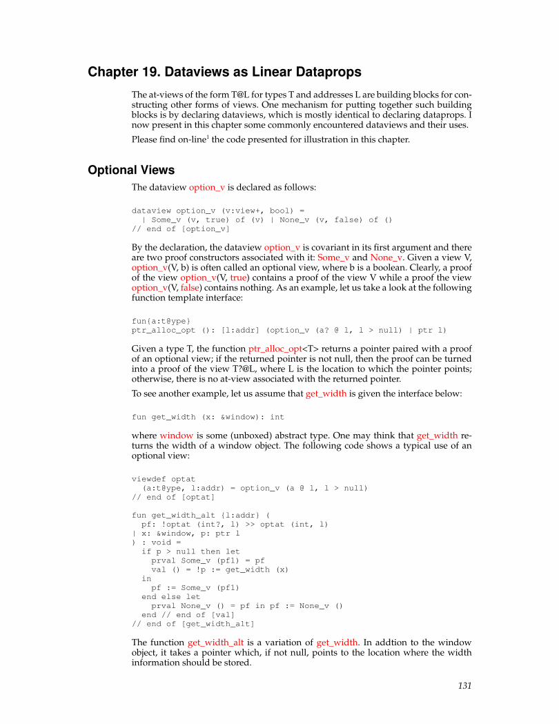
Chapter 19. Dataviews as Linear Dataprops
The at-views of the form T@L for types T and addresses L are building blocks for con-structing other forms of views. One mechanism for putting together such buildingblocks is by declaring dataviews, which is mostly identical to declaring dataprops. Inow present in this chapter some commonly encountered dataviews and their uses.
Please find on-line1 the code presented for illustration in this chapter.
Optional ViewsThe dataview option_v is declared as follows:
dataview option_v (v:view+, bool) =| Some_v (v, true) of (v) | None_v (v, false) of ()
// end of [option_v]
By the declaration, the dataview option_v is covariant in its first argument and thereare two proof constructors associated with it: Some_v and None_v. Given a view V,option_v(V, b) is often called an optional view, where b is a boolean. Clearly, a proofof the view option_v(V, true) contains a proof of the view V while a proof the viewoption_v(V, false) contains nothing. As an example, let us take a look at the followingfunction template interface:
fun{a:t@ype}ptr_alloc_opt (): [l:addr] (option_v (a? @ l, l > null) | ptr l)
Given a type T, the function ptr_alloc_opt<T> returns a pointer paired with a proofof an optional view; if the returned pointer is not null, then the proof can be turnedinto a proof of the view T?@L, where L is the location to which the pointer points;otherwise, there is no at-view associated with the returned pointer.
To see another example, let us assume that get_width is given the interface below:
fun get_width (x: &window): int
where window is some (unboxed) abstract type. One may think that get_width re-turns the width of a window object. The following code shows a typical use of anoptional view:
viewdef optat(a:t@ype, l:addr) = option_v (a @ l, l > null)
// end of [optat]
fun get_width_alt {l:addr} (pf: !optat (int?, l) >> optat (int, l)
| x: &window, p: ptr l) : void =if p > null then letprval Some_v (pf1) = pfval () = !p := get_width (x)
inpf := Some_v (pf1)
end else letprval None_v () = pf in pf := None_v ()
end // end of [val]// end of [get_width_alt]
The function get_width_alt is a variation of get_width. In addtion to the windowobject, it takes a pointer which, if not null, points to the location where the widthinformation should be stored.
131

Chapter 19. Dataviews as Linear Dataprops
Please find the entirety of the above presented code on-line2.
Linear ArraysUnlike in most programming languages, arrays are not a primitive data structurein ATS. More specifically, persistent arrays can be implemented based on linear ar-rays, which allow for being freed safely by the programmer, and linear arrays canbe implemented based on at-views. Intuitively, the view for an array containing Nelements of type T consists of N at-views: T@L
0, T@L
1, ..., and T@L
N-1, where L
0is
the starting address of the array and each subsequent L equals the previous one plusthe size of T, that is, the number of bytes needed to store a value of the type T. Thefollowing declared dataview array_v precisely captures the intuituion:
dataview array_v(a:t@ype+, int(*size*), addr(*beg*)) =| {n:nat} {l:addr}array_v_cons (a, n+1, l) of (a @ l, array_v (a, n, l+sizeof(a)))
| {l:addr} array_v_nil (a, 0, l)// end of [array_v]
Given a type T, an integer N and an address L, array_v(T, N, L) is a view for the arraystarting at L that contains N elements of the type T. As can be readily expected, thefunction templates for array accessing and array updating are given the followinginterfaces:
fun{a:t@ype}arrget {n,i:nat | i < n} {l:addr}(pf: !array_v (a, n, l) | p: ptr l, i: int i): a
// end of [arrget]
fun{a:t@ype}arrset {n,i:nat | i < n} {l:addr}(pf: !array_v (a, n, l) | p: ptr l, i: int i, x: a): void
// end of [arrset]
Before implementing arrget and arrset, I present as follows some code that imple-ments a function template to access the first element of a nonempty array:
fun{a:t@ype}arrgetfst {n:pos} {l:addr} (pf: !array_v (a, n, l) | p: ptr l
) : a = x where {prval array_v_cons (pf1, pf2) = pf// pf1: a @ l; pf2: array_v (a, n-1, l+sizeof(a))val x = !pprval () = pf := array_v_cons (pf1, pf2)
} // end of [arrgetfst]
Obviously, the function template arrget can be implemented based on arrgetfst:
implement{a}arrget (pf | p, i) =if i > 0 then letprval array_v_cons (pf1, pf2) = pfval x = arrget (pf2 | p+sizeof<a>, i-1)prval () = pf := array_v_cons (pf1, pf2)
inx
end elsearrgetfst (pf | p)
// end of [if]
132

Chapter 19. Dataviews as Linear Dataprops
This implementation is of time-complexity O(n), and it is tail-recursive (after theproofs are erased). However, the very point of having arrays is to support O(1)-timeaccessing and updating operations. My initial effort spent on implementing such op-erations immediately dawned on me the need to construct proof functions for sup-porting view changes (of no run-time cost).
Clearly, an array starting at L that contains N elements of type T can also be thoughtof as two arrays: one starting at L that contains I elements while the other startingat L+I*sizeof(T) that contains N-I elements, where I is an natural number less that orequal to N. Formally, this statement can be encoded in the type of the proof functionarray_v_split:
prfun array_v_split{a:t@ype} {n,i:nat | i <= n} {l:addr} {ofs:int} (pfmul: MUL (i, sizeof(a), ofs), pfarr: array_v (a, n, l)
) : (array_v (a, i, l), array_v (a, n-i, l+ofs))
The other direction of the above statement can be encoded in the type of the prooffunction array_v_unsplit:
prfun array_v_unsplit{a:t@ype} {n1,n2:nat} {l:addr} {ofs:int} (pfmul: MUL (n1, sizeof(a), ofs)
, pf1arr: array_v (a, n1, l), pf2arr: array_v (a, n2, l+ofs)) : array_v (a, n1+n2, l)
With array_v_split and array_v_unsplit, we can readily give implementations ofarrget and arrset that are O(1)-time:
implement{a}arrget (pf | p, i) = x where {val tsz = int1_of_size1 (sizeof<a>)val (pfmul | ofs) = i imul2 tszprval (pf1, pf2) = array_v_split {a} (pfmul, pf)prval array_v_cons (pf21, pf22) = pf2val x = ptr_get1<a> (pf21 | p+ofs)prval pf2 = array_v_cons (pf21, pf22)prval () = pf := array_v_unsplit {a} (pfmul, pf1, pf2)
} // end of [arrget]
implement{a}arrset (pf | p, i, x) = () where {val tsz = int1_of_size1 (sizeof<a>)val (pfmul | ofs) = i imul2 tszprval (pf1, pf2) = array_v_split {a} (pfmul, pf)prval array_v_cons (pf21, pf22) = pf2val () = ptr_set1<a> (pf21 | p+ofs, x)prval pf2 = array_v_cons (pf21, pf22)prval () = pf := array_v_unsplit {a} (pfmul, pf1, pf2)
} // end of [arrset]
Note that the function int1_of_size1 is called to turn a size (i.e., an integer of thetype size_t) into an int (i.e., an integer of the type int). Of course, the proof functionsarray_v_split and array_v_split are still to be implemented, which I will do whencovering the topic of view change.
Given a type T and a natural number N, a proof of the view array_v(T?, N, L) forsome address L can be obtained and released by calling the functions malloc and free,respectively, which are to be explained in details elsewhere. I now give as follows animplemention of a function template for array intialization:
typedef natLt (n:int) = [i:nat | i < n] int (i)
133

Chapter 19. Dataviews as Linear Dataprops
fun{a:t@ype}array_ptr_tabulate{n:nat} {l:addr} (pf: !array_v (a?,n,l) >> array_v (a,n,l)
| p: ptr (l), n: int (n), f: natLt(n) -<cloref1> a) : void = letfun loop {i:nat | i <= n} {l:addr} .<n-i>. (pf: !array_v (a?,n-i,l) >> array_v (a,n-i,l)
| p: ptr l, n: int n, f: natLt(n) -<cloref1> a, i: int i) : void =if i < n then letprval array_v_cons (pf1, pf2) = pfval () = !p := f (i)val () = loop (pf2 | p+sizeof<a>, n, f, i+1)
inpf := array_v_cons (pf1, pf2)
end else letprval array_v_nil () = pf in pf := array_v_nil {a} ()
end // end of [if]// end of [loop]
inloop (pf | p, n, f, 0)
end // end of [array_ptr_tabulate]
Given a natural number n, the type natLt(n) is for all natural numbers less than n.Given a type T, the function array_ptr_tabulate<T> takes a pointer to an uninitializedarray, the size of the array and a function f that maps each natural number less thann to a value of the type T, and it initializes the array with the sequence of values off(0), f(1), ..., and f(n-1). In other words, the array contains a tabulation of the givenfunction f after the initialization is over.
Given a type T and an integer N, @[T][N] is a built-in type in ATS for N consecutivevalues of the type T. Therefore, the at-view @[T][N]@L for any given address L isequivalent to the array-view array_v(T, N, L). By making use of the feature of call-by-reference, we can also assign the following interfaces to the previously presentedfunctions arrget and arrset:
fun{a:t@ype}arrget {n,i:nat | i < n} (A: &(@[a][n]), i: int i): a
fun{a:t@ype}arrset {n,i:nat | i < n} (A: &(@[a][n]), i: int i, x: a): void
These interfaces are more concise as they obviate the need to mention explicitlywhere the array argument is located.
Please find the entirety of the above presented code on-line3.
Singly-Linked ListsThe following dataview slseg_v captures the notion of a singly-linked list segment:
dataviewslseg_v (a:t@ype+ // covariant argument
, int(*len*), addr(*beg*), addr(*end*)) =| {l:addr} slseg_v_nil (a, 0, l, l) of ()| {n:nat} {l_fst:agz} {l_nxt,l_end:addr}slseg_v_cons (a, n+1, l_fst, l_end) of((a, ptr l_nxt) @ l_fst, slseg_v (a, n, l_nxt, l_end))
134

Chapter 19. Dataviews as Linear Dataprops
// end of [slseg]_v
There are two proof constructors slseg_v_nil and slseg_v_cons associated withslseg_v, which are assigned the following types:
slseg_v_nil :{a:t@ype} {l:addr} () -> slseg_v (a, 0, l, l)
slseg_v_cons :{a:t@ype} {n:nat} {l_fst:agz} {l_nxt,l_end:addr}((a, ptr l_nxt) @ l_fst, slseg_v (a, l_nxt, l_end)) -> slseg_v (a, n+1, l_fst, l_end)
Note that agz is a subset sort for addresses that are not null. Given a type T, a naturalnumber N and two addresses L1 and L2, the view slseg_v (T, N, L1, L2) is for a singly-linked list segment containing N elements of the type T that starts at L1 and finishesat L2. In the case where L2 is the null pointer, then the list segment is considered alist as is formally defined below:
viewdef sllst_v(a:t@ype, n:int, l:addr) = slseg_v (a, n, l, null)
// end of [sllst_v]
Given a type T, a pointer pointing to L plus a proof of the view sllst_v(T, N, L) forsome natural number N is essentially the same as a pointer to a struct of the followingdeclared type sllst_struct in C:
typedef struct sllst {T data ; /* [T] matches the corresponding type in ATS */struct sllst *next ; /* pointing to the tail of the list */
} sllst_struct ;
Let us now see a simple example involving singly-linked lists:
fn{a:t@ype}sllst_ptr_length{n:nat} {l:addr} (pflst: !sllst_v (a, n, l) | p: ptr l
) : int (n) = letfun loop {i,j:nat} {l:addr} .<i>. (pflst: !sllst_v (a, i, l) | p: ptr l, j: int (j)
) : int (i+j) =if p > null then letprval slseg_v_cons (pfat, pf1lst) = pflstval res = loop (pf1lst | !p.1, j+1) // !p.1 points to the tailprval () = pflst := slseg_v_cons (pfat, pf1lst)
inres
end else let // the length of a null list is 0prval slseg_v_nil () = pflst in pflst := slseg_v_nil (); j
end (* end of [if] *)// end of [loop]
inloop (pflst | p, 0)
end // end of [sllst_ptr_length]
The function template sllst_ptr_length computes the length of a given singly-linkedlist. Note that the inner function loop is tail-recursive. The above implementation ofsllst_ptr_length essentially corresponds to the following implementation in C:
int sllst_ptr_length (sllst_struct *p) {int res = 0 ;while (p != NULL) { res = res + 1 ; p = p->next ; }return res ;
135

Chapter 19. Dataviews as Linear Dataprops
} // end of [sllst_ptr_length]
As another example, the following function template sllst_ptr_reverse turns a givenlinked list into its reverse:
fn{a:t@ype}sllst_ptr_reverse{n:nat} {l:addr} (pflst: sllst_v (a, n, l) | p: ptr l
) : [l:addr] (sllst_v (a, n, l) | ptr l) = letfun loop{n1,n2:nat}{l1,l2:addr} .<n1>. (pf1lst: sllst_v (a, n1, l1)
, pf2lst: sllst_v (a, n2, l2)| p1: ptr l1, p2: ptr l2) : [l:addr] (sllst_v (a, n1+n2, l) | ptr l) =if p1 > null then letprval slseg_v_cons (pf1at, pf1lst) = pf1lstval p1_nxt = !p1.1val () = !p1.1 := p2
inloop (pf1lst, slseg_v_cons (pf1at, pf2lst) | p1_nxt, p1)
end else letprval slseg_v_nil () = pf1lst in (pf2lst | p2)
end // end of [if]inloop (pflst, slseg_v_nil | p, null)
end // end of [sllst_ptr_reverse]
By translating the tail-recursive function loop into a while-loop, we can readily turnthe implementation of sllst_ptr_reverse in ATS into the following implementation inC:
sllst_struct *sllst_ptr_reverse (sllst_struct *p) {sllst_struct *tmp, *res = NULL ;while (p != NULL) {tmp = p->next ; p->next = res ; res = p ; p = tmp ;
}return res ;
} // end of [sllst_ptr_reverse]
Let us see yet another example. List concatenation is a common operation on lists.This time, we first give an implementation of list concatenation in C:
sllst_struct *sllst_ptr_append(sllst_struct *p, sllst_struct *q) {sllst_struct *p1 = p ;if (p1 == NULL) return q ;while (p1->next != NULL) p1 = p1->next ; p1->next = q ;return p ;
} // end of [sllst_ptr_append]
The algorithm is straightforward. If p is null, then q is returned. Otherwise, the lastnode in the list pointed to by p is first found and its field of the name next thenreplaced with q. This implementation of sllst_ptr_append in C can be translated di-rectly into to following one in ATS:
fn{a:t@ype}sllst_ptr_append{n1,n2:nat} {l1,l2:addr} (pf1lst: sllst_v (a, n1, l1)
, pf2lst: sllst_v (a, n2, l2)
136
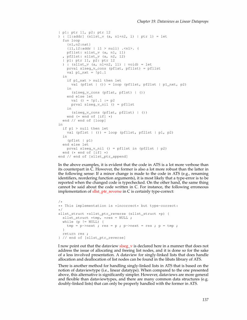
Chapter 19. Dataviews as Linear Dataprops
| p1: ptr l1, p2: ptr l2) : [l:addr] (sllst_v (a, n1+n2, l) | ptr l) = letfun loop{n1,n2:nat}{l1,l2:addr | l1 > null} .<n1>. (pf1lst: sllst_v (a, n1, l1)
, pf2lst: sllst_v (a, n2, l2)| p1: ptr l1, p2: ptr l2) : (sllst_v (a, n1+n2, l1) | void) = letprval slseg_v_cons (pf1at, pf1lst) = pf1lstval p1_nxt = !p1.1
inif p1_nxt > null then letval (pflst | ()) = loop (pf1lst, pf2lst | p1_nxt, p2)
in(slseg_v_cons (pf1at, pflst) | ())
end else letval () = !p1.1 := p2prval slseg_v_nil () = pf1lst
in(slseg_v_cons (pf1at, pf2lst) | ())
end (* end of [if] *)end // end of [loop]
inif p1 > null then letval (pflst | ()) = loop (pf1lst, pf2lst | p1, p2)
in(pflst | p1)
end else letprval slseg_v_nil () = pf1lst in (pf2lst | p2)
end (* end of [if] *)end // end of [sllst_ptr_append]
In the above examples, it is evident that the code in ATS is a lot more verbose thanits counterpart in C. However, the former is also a lot more robust than the latter inthe following sense: If a minor change is made to the code in ATS (e.g., renamingidentifiers, reordering function arguments), it is most likely that a type-error is to bereported when the changed code is typechecked. On the other hand, the same thingcannot be said about the code written in C. For instance, the following erroneousimplementation of sllst_ptr_reverse in C is certainly type-correct:
/*** This implementation is *incorrect* but type-correct:*/sllst_struct *sllst_ptr_reverse (sllst_struct *p) {
sllst_struct *tmp, *res = NULL ;while (p != NULL) {tmp = p->next ; res = p ; p->next = res ; p = tmp ;
}return res ;
} // end of [sllst_ptr_reverse]
I now point out that the dataview slseg_v is declared here in a manner that does notaddress the issue of allocating and freeing list nodes, and it is done so for the sakeof a less involved presentation. A dataview for singly-linked lists that does handleallocation and deallocation of list nodes can be found in the libats library of ATS.
There is another method for handling singly-linked lists in ATS that is based on thenotion of dataviewtype (i.e., linear datatype). When compared to the one presentedabove, this alternative is significantly simpler. However, dataviews are more generaland flexible than dataviewtypes, and there are many common data structures (e.g.doubly-linked lists) that can only be properly handled with the former in ATS.
137
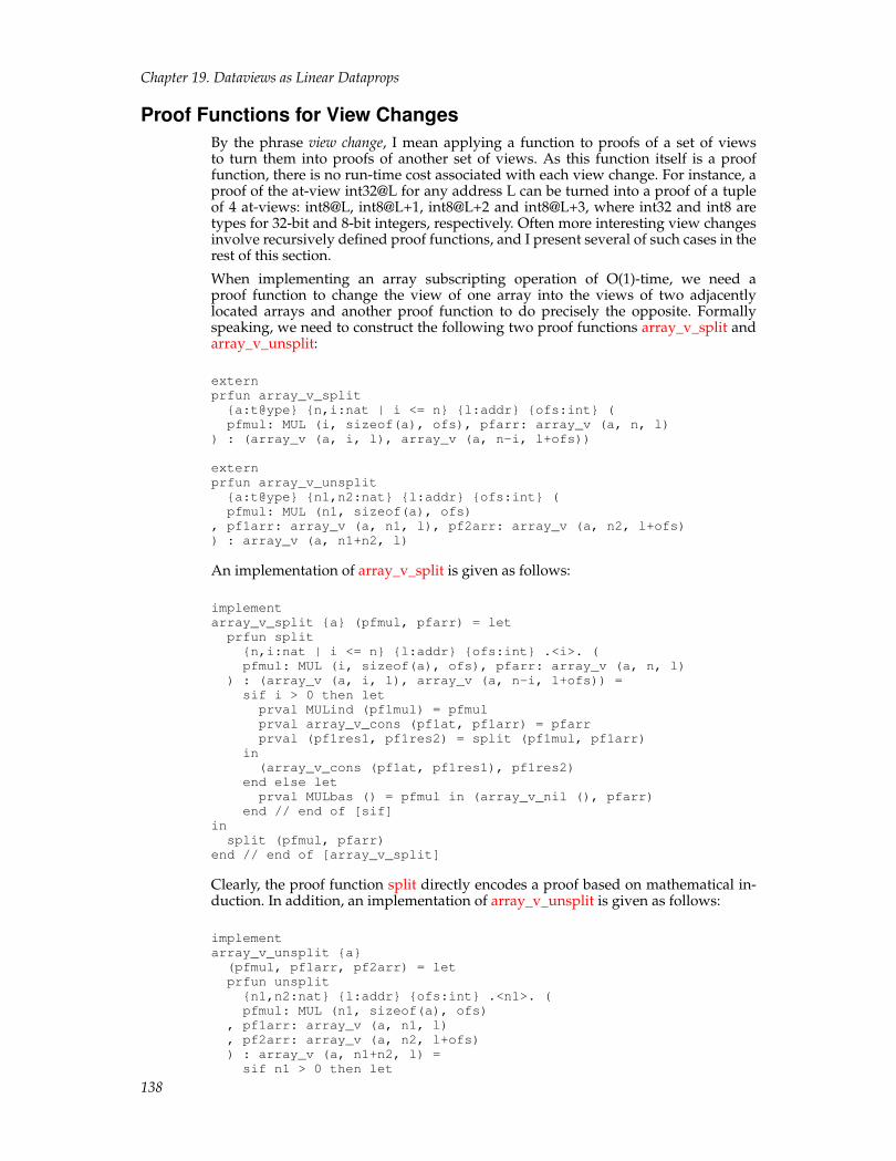
Chapter 19. Dataviews as Linear Dataprops
Proof Functions for View ChangesBy the phrase view change, I mean applying a function to proofs of a set of viewsto turn them into proofs of another set of views. As this function itself is a prooffunction, there is no run-time cost associated with each view change. For instance, aproof of the at-view int32@L for any address L can be turned into a proof of a tupleof 4 at-views: int8@L, int8@L+1, int8@L+2 and int8@L+3, where int32 and int8 aretypes for 32-bit and 8-bit integers, respectively. Often more interesting view changesinvolve recursively defined proof functions, and I present several of such cases in therest of this section.
When implementing an array subscripting operation of O(1)-time, we need aproof function to change the view of one array into the views of two adjacentlylocated arrays and another proof function to do precisely the opposite. Formallyspeaking, we need to construct the following two proof functions array_v_split andarray_v_unsplit:
externprfun array_v_split{a:t@ype} {n,i:nat | i <= n} {l:addr} {ofs:int} (pfmul: MUL (i, sizeof(a), ofs), pfarr: array_v (a, n, l)
) : (array_v (a, i, l), array_v (a, n-i, l+ofs))
externprfun array_v_unsplit{a:t@ype} {n1,n2:nat} {l:addr} {ofs:int} (pfmul: MUL (n1, sizeof(a), ofs)
, pf1arr: array_v (a, n1, l), pf2arr: array_v (a, n2, l+ofs)) : array_v (a, n1+n2, l)
An implementation of array_v_split is given as follows:
implementarray_v_split {a} (pfmul, pfarr) = letprfun split{n,i:nat | i <= n} {l:addr} {ofs:int} .<i>. (pfmul: MUL (i, sizeof(a), ofs), pfarr: array_v (a, n, l)
) : (array_v (a, i, l), array_v (a, n-i, l+ofs)) =sif i > 0 then letprval MULind (pf1mul) = pfmulprval array_v_cons (pf1at, pf1arr) = pfarrprval (pf1res1, pf1res2) = split (pf1mul, pf1arr)
in(array_v_cons (pf1at, pf1res1), pf1res2)
end else letprval MULbas () = pfmul in (array_v_nil (), pfarr)
end // end of [sif]insplit (pfmul, pfarr)
end // end of [array_v_split]
Clearly, the proof function split directly encodes a proof based on mathematical in-duction. In addition, an implementation of array_v_unsplit is given as follows:
implementarray_v_unsplit {a}(pfmul, pf1arr, pf2arr) = letprfun unsplit{n1,n2:nat} {l:addr} {ofs:int} .<n1>. (pfmul: MUL (n1, sizeof(a), ofs)
, pf1arr: array_v (a, n1, l), pf2arr: array_v (a, n2, l+ofs)) : array_v (a, n1+n2, l) =sif n1 > 0 then let
138

Chapter 19. Dataviews as Linear Dataprops
prval MULind (pf1mul) = pfmulprval array_v_cons (pf1at, pf1arr) = pf1arrprval pfres = unsplit (pf1mul, pf1arr, pf2arr)
inarray_v_cons (pf1at, pfres)
end else letprval MULbas () = pfmulprval array_v_nil () = pf1arr
inpf2arr
end // end of [sif]inunsplit (pfmul, pf1arr, pf2arr)
end // end of [array_v_unsplit]
The proof function unsplit also directly encodes a proof based on mathematical in-duction.
Let us now see an even more interesting proof function for performing view change.The interface of the proof function array_v_takeout is given as follows:
externprfun array_v_takeout{a:t@ype} {n,i:nat | i < n} {l:addr} {ofs:int} (pfmul: MUL (i, sizeof(a), ofs), pfarr: array_v (a, n, l)
) : (a @ l+ofs, a @ l+ofs -<lin,prf> array_v (a, n, l))
Note that the following type is for a linear proof function that takes a proof of anat-view to return a proof of an array-view:
a @ l+ofs -<lin,prf> array_v (a, n, l)
As such a function essentially represents an array with one missing cell, we maysimply say that array_v_takeout turns the view of an array into an at-view (for onecell) and a view for the rest of the array. By making use of array_v_takeout, we cangive another implementation of arrget:
implement{a}arrget (pf | p, i) = x where {val tsz = int1_of_size1 (sizeof<a>)val (pfmul | ofs) = i imul2 tszprval (pf1, fpf2) = array_v_takeout {a} (pfmul, pf)val x = ptr_get1<a> (pf1 | p+ofs)prval () = pf := fpf2 (pf1) // putting the cell and the rest together
} // end of [arrget]
The proof function array_v_takeout can be implemented as follows:
implementarray_v_takeout{a} (pfmul, pfarr) = letprfun takeout{n,i:nat | i < n} {l:addr} {ofs:int} .<i>. (pfmul: MUL (i, sizeof(a), ofs), pfarr: array_v (a, n, l)
) : (a @ l+ofs, a @ l+ofs -<lin,prf> array_v (a, n, l)) = letprval array_v_cons (pf1at, pf1arr) = pfarr
insif i > 0 then letprval MULind (pf1mul) = pfmulprval (pfres, fpfres) = takeout (pf1mul, pf1arr)
in(pfres, llam (pfres) => array_v_cons (pf1at, fpfres (pfres)))
end else let
139

Chapter 19. Dataviews as Linear Dataprops
prval MULbas () = pfmulin(pf1at, llam (pf1at) => array_v_cons (pf1at, pf1arr))
end // end of [sif]end // end of [takeout]
intakeout (pfmul, pfarr)
end // end of [array_v_takeout]
Note that llam is a keyword for forming linear functons. Once a linear function isapplied, it is consumed and the resource in it, if not reclaimed, moves into the resultit returns.
The proof functions presented so far for view changes are all manipulating array-views. The following one is different in this regard as it combines two views forsingly-linked list segments into one:
prfun slseg_v_unsplit{a:t@ype} {n1,n2:nat} {l1,l2,l3:addr} (pf1lst: slseg_v (a, n1, l1, l2), pf2lst: slseg_v (a, n2, l2, l3)
) : slseg_v (a, n1+n2, l1, l3)
The type of slseg_v_unsplit essentially states that a list segment from L1 to L2 thatis of length N1 and another list segment from L2 to L3 that is of length N2 can bethought of as a list segment from L1 to L3 that is of length N1+N2. The followingimplementation of slseg_v_unsplit is largely parallel to that of array_v_unsplit:
implementslseg_v_unsplit {a}(pf1lst, pf2lst) = letprfun unsplit{n1,n2:nat} {l1,l2,l3:addr} .<n1>. (pf1lst: slseg_v (a, n1, l1, l2), pf2lst: slseg_v (a, n2, l2, l3)
) : slseg_v (a, n1+n2, l1, l3) =sif n1 > 0 then letprval slseg_v_cons (pf1at, pf1lst) = pf1lst
inslseg_v_cons (pf1at, unsplit (pf1lst, pf2lst))
end else letprval slseg_v_nil () = pf1lst in pf2lst
end // end of [sif]inunsplit (pf1lst, pf2lst)
end // end of [slseg_v_unsplit]
The reader may find it interesting to give an implementation of sllst_ptr_append bymaking use of slseg_v_unsplit.
Please find on-line the files array.dats4 and sllst.dats5, which contains the code em-ployed for illustration in this section.
Example: QuicksortQuicksort is a commonly employed sorting algorithm in practice. Given an array ofn elements for some n > 0 and an ordering on these elements, the algorithm choosesone element in a more or less random fashion and then uses the chosen element as apivot to shuffle the rest of the array into two parts separated by the pivot such thatone part consists of all the elements that are less than or equal to the pivot (accordingto the given ordering) and the other part consists of the complement, that is, all theelements that are greater than the pivot; then the algorithm is applied recursively toeach part unless it is empty. It is straightforward to see that the array is sorted afterthe algorithm terminates. In terms of time-complexity, quicksort is quadratic in the
140

Chapter 19. Dataviews as Linear Dataprops
worst case and log-linear on average. Also, quicksort is not a stable sorting algorithmin the sense that the order of two equal elements may change after sorting.
The following function npivot returns the index of the element chosen to be the pivot:
fun{a:t@ype}npivot {n:pos} {l:addr} (pf: !array_v (a, n, l) | p: ptr l, n: int (n), cmp: cmp (a)
) : natLt (n) = n/2
For simplicity, the index of the pivot for an array of size n is always n/2 (whereinteger division is used). Often a more elaborate method is to choose the index among0, n/2 and n-1 such that the element stored at that index is between the elementsstored at the other two indexes. Another possibility is to choose the index of thepivot based on a pseudo random number generator.
The function template array_ptr_exch for exchanging two elements in a given arrayis assgined the following interface:
externfun{a:t@ype}array_ptr_exch {n:nat} {l:addr} (pf: !array_v (a, n, l) | p: ptr l, i: natLt n, j: natLt n
) : void // end of [array_ptr_exch]
I give no implementation of array_ptr_exch here as the reader should have no diffi-culty constructing one by now.
Given an array of elements, its size, an ordering on the elements and a pivot, thefollowing function template split turns the array into two subarrays such that onesubarray consists of all the elements in the array that are less than or equal to thepivot and the other subarray consists of the complement; it then returns the size ofthe first subarray plus proofs of the views of the two subarrays (as well as a proof forhandling multiplication).
externfun{a:t@ype}split {n:nat} {l:addr} (pf: array_v (a, n, l) | p: ptr l, n: int n, cmp: cmp a, piv: &a
) : [n1,n2:nat | n1+n2==n] [ofs:int] (MUL (n1, sizeof(a), ofs), array_v (a, n1, l), array_v (a, n2, l+ofs) | int n1
) // end of [split]
I postpone implementing split for the moment. Instead, let us first see an implemen-tation of quicksort based on split:
fun{a:t@ype}qsort {n:nat} {l:addr} .<n>. (pfarr: !array_v (a, n, l) | p: ptr l, n: int (n), cmp: cmp (a)
) : void =if n > 0 then letval tsz = int1_of_size1 (sizeof<a>)val npiv = npivot (pfarr | p, n, cmp)val () = array_ptr_exch (pfarr | p, 0, npiv) // move the pivot to the front
//val p1 = p+tszprval array_v_cons (pfat, pf1arr) = pfarrval (pfmul, pf1arr_lte, pf1arr_gt | n1) = split (pf1arr | p1, n-1, cmp, !p)
// combining the pivot with the first segmentprval pf1arr_lte = array_v_cons (pfat, pf1arr_lte)
// exchanging the pivot with the last element in the first segmentval () = array_ptr_exch (pf1arr_lte | p, 0, n1)
// separating the pivot from all the elements in front of it
141
Chapter 19. Dataviews as Linear Dataprops
prval (pf1arr_lte, pflast) = array_v_split {a} (pfmul, pf1arr_lte)val () = qsort (pf1arr_lte | p, n1, cmp) // recursive all to qsort
// combining the pivot with all the elements in front of itprval pf1arr_lte = array_v_unsplit {a} (pfmul, pf1arr_lte, pflast)
//val (pfmul_alt | ofs) = n1 imul2 tszprval () = mul_isfun (pfmul, pfmul_alt)val () = qsort (pf1arr_gt | p1+ofs, n-n1-1, cmp) // recursive call to qsort
// combining the first and the second segments togetherprval () = pfarr := array_v_unsplit {a} (MULind (pfmul), pf1arr_lte, pf1arr_gt)
in// nothing
end else () // empty array// end of [qsort]
The comments given in the implementation of qsort should make it rather clear howquicksort formally operates on a given array.
Let us now implement the function template split. Given an array, one common ap-proach is to have two pointers pointing to the first and last elements of the array; thefront pointer moves forward until an element that is not less than or equal to the pivotis encountered; the rear pointer moves backward until an element that is not greaterthan the pivot is encountered; the elements pointed to by the front and rear pointersare exchanged and the process is repeated; the process finishes at the moment whenthe front pointer either encounters or crosses over the rear one. As it is considerablyinvolved to present an implementation based on this approach, I will use an alterna-tive one, which I learned from the K&R book on the C programming language. Thisalternative approach starts with two pointers p1 and p2 pointing to the beginningof the given array and maintains the invariant that each element between p1 and p2is greater than the pivot; first p2 moves forward until an element that is less thanor equal to the pivot is encountered; then the elements stored at p1 and p2 are ex-changed and both p1 and p2 move forward by one unit; the process repeats until p2reaches the end of the array. For a slightly cleaner presentation, p1 is represented as areal pointer (p) in the implementation of the following inner function loop while p2is represented as an integer (k):
implement{a}split {n} (pfarr | p, n, cmp, piv
) = letfun loop{n1:nat}{k:nat | n1+k <= n}{l:addr} {ofs:int} .<n-n1-k>. (pfmul: MUL (n1, sizeof(a), ofs)
, pf1arr: array_v (a, n1, l), pf2arr: array_v (a, n-n1, l+ofs)| p: ptr (l+ofs), n: int n, n1: int n1, k: int k, cmp: cmp(a), piv: &a) : [n1,n2:nat | n1+n2==n] [ofs:int] (MUL (n1, sizeof(a), ofs), array_v (a, n1, l), array_v (a, n2, l+ofs)
| int (n1)) = // [loop] is tail-recursiveif n1+k < n then letval (pfat, fpf2 | pk) = array_ptr_takeout (pf2arr | p, k)val sgn = compare (!pk, piv, cmp)prval () = pf2arr := fpf2 (pfat)
inif sgn > 0 thenloop (pfmul, pf1arr, pf2arr | p, n, n1, k+1, cmp, piv)
else letval () = array_ptr_exch (pf2arr | p, 0, k) // no work is done if k = 0prval array_v_cons (pfat, pf2arr) = pf2arrprval () = pf1arr := array_v_extend {a} (pfmul, pf1arr, pfat)
in
142

Chapter 19. Dataviews as Linear Dataprops
loop (MULind (pfmul), pf1arr, pf2arr | p+sizeof<a>, n, n1+1, k, cmp, piv)end (* end of [if] *)
end else (pfmul, pf1arr, pf2arr | n1
) // end of [if]inloop (MULbas (), array_v_nil (), pfarr | p, n, 0, 0, cmp, piv)
end // end of [split]
Note the proof function array_v_extend is given the following interface:
prfun array_v_extend{a:t@ype} {n:nat} {l:addr} {ofs:int} (pfmul: MUL (n, sizeof(a), ofs), pfarr: array_v (a, n, l), pfat: a @ l+ofs
) : array_v (a, n+1, l)
This proof function can be thought of as a special case of array_v_unsplit where thesecond array is a singleton, that is, it contains exactly one element.
Please find the entire code in this section plus some additional code for testing on-line6.
Notes1. http://www.ats-lang.org/DOCUMENT/INTPROGINATS/CODE/CHAPTER_DATAVIEWS/
2. http://www.ats-lang.org/DOCUMENT/INTPROGINATS/CODE/CHAPTER_DATAVIEWS/optview.dats
3. http://www.ats-lang.org/DOCUMENT/INTPROGINATS/CODE/CHAPTER_DATAVIEWS/array.dats
4. http://www.ats-lang.org/DOCUMENT/INTPROGINATS/CODE/CHAPTER_DATAVIEWS/array.dats
5. http://www.ats-lang.org/DOCUMENT/INTPROGINATS/CODE/CHAPTER_DATAVIEWS/sllst.dats
6. http://www.ats-lang.org/DOCUMENT/INTPROGINATS/CODE/CHAPTER_DATAVIEWS/quicksort.dats
143
Chapter 19. Dataviews as Linear Dataprops
144

Chapter 20. Dataviewtypes as Linear Datatypes
A dataviewtype can be thought of as a linear version of datatype. To a large extent, itis a combination of a datatype and a dataview. This programming feature is primar-ily introduced into ATS for the purpose of providing the kind convenience of patternmatching associated with datatypes while incurring no need for run-time garbagecollection (GC). In a situation where GC must be reduced or even completely elimi-nated, dataviewtypes can often chosen as a replacement for datatypes. I now presentin this chapter some commonly encountered dataviewtypes and their uses.
Linear Optional ValuesWhen an optional value is created, it is most likely to be used immediately and thendiscarded. If such a value is assigned a linear type, then the memory allocated forstoring it can be efficiently reclaimed. The dataviewtype option_vt for linear optionalvalues is declared as follows:
dataviewtyeoption_vt (a:t@ype+, bool) =| Some_vt (a, true) of a | None_vt (a, false) of ()
// end of [option_vt]
viewtypedefOption_vt (a:t@ype) = [b:bool] option_vt (a, b)
By the declaration, the dataviewtype option_vt is covariant in its first argument andthere are two data constructors Some_vt and None_vt associated with it. In the fol-lowing example, find_rightmost tries to find the rightmost element in a list that sat-isfies a given predicate:
fun{a:t@ype}find_rightmost {n:nat} .<n>.(xs: list (a, n), P: (a) -<cloref> bool): Option_vt (a) =case+ xs of| list_cons (x, xs) => let
val opt = find_rightmost (xs, P)incase opt of| ~None_vt () => if P (x) then Some_vt (x) else None_vt ()| _ => opt
end // end of [list_cons]| list_nil () => None_vt ()
// end of [find_rightmost]
Note that the tilde symbol (~) in front of the pattern None_vt() indicates that thememory for the node that matches the pattern is freed before the body of the matchedclause is evaluated. In this case, no memory is actually freed as None_vt is mappedto the null pointer. I will soon give more detailed explanation about freeing memoryallocated for constructors associated with dataviewtypes.
As another example, the following function template list_optcons tries to construct anew list with its head element extracted from a given optional value:
fn{a:t@ype}list_optcons {b:bool} {n:nat} (opt: option_vt (a, b), xs: list (a, n)
) : list (a, n+int_of_bool(b)) =case+ opt of| ~Some_vt (x) => list_cons (x, xs) | ~None_vt () => xs
// end of [list_optcons]
145
Chapter 20. Dataviewtypes as Linear Datatypes
The symbol int_of_bool stands for a built-in static function in ATS that maps trueand false to 1 and 0, respectively. What is special here is that the first argument oflist_optcons, which is linear, is consumed after a call to list_optcons returns and thememory it occupies is reclaimed.
Linear ListsA linear list is essentially the same as a singly-linked list depicted by the dataviewsllst_v. However, memory allocation and deallocation of list nodes that were nothandled previously are handled this time. The following declaration introduces adataviewtype list_vt, which forms a boxed type (of the sort viewtype) when appliedto a type and an integer:
dataviewtypelist_vt (a:t@ype+, int) =| {n:nat}list_vt_cons (a, n+1) of (a, list_vt (a, n))
| list_vt_nil (a, 0) of ()// end of [list_vt]
Assume that a data constructor named foo is associated with a dataviewtype.Then there is a viewtype construtor of the name foo_unfold that takes n addressesto form a viewtype, where n is the arity of foo. For instance, there is a viewtypeconstructor list_vt_cons_unfold that takes two address L0 and L1 to form aviewtype list_vt_cons_unfold(L0, L1). This viewtype is for a list node created by acall to list_vt_cons such that the two arguments of list_vt_cons are located at L0 andL1 while the proofs for the at-views associated with L0 and L1 are put in the storefor currently available proofs.
Given a type T and an integer I, the viewtype list_vt(T, I) is for linear lists of length Iin which each element is assigned the type T. The following function template lengthcomputes the length of a given linear list:
fn{a:t@ype}length {n:nat}(xs: !list_vt (a, n)): int n = letfun loop{i,j:nat | i+j==n} .<i>.(xs: !list_vt (a, i), j: int j): int (n) =case+ xs of| list_vt_cons (_, !p_xs1) => let
val n = loop (!p_xs1, j+1); val () = fold@ (xs) in nend // end of [list_vt_cons]
| list_vt_nil () => (fold@ (xs); j)// end of [loop]
inloop (xs, 0)
end // end of [length]
The interface of length indicates that length<T> returns an integer equal to I whenapplied to a list of the type list_vt(T, I), where T and I are a type and an integer, re-spectively. Note that the symbol ! in front of the type of a function argument indicatesthat the argument is call-by-value and it is preserved after a call to the function.
What is particularly interesting here is the way in which pattern matching on a valueof a dataviewtype works. In the body of the inner function loop, the type of xschanges to list_vt_cons_unfold(L1, L2) for some addresses L1 and L2 when it matchesthe pattern list_vt_cons(_, !p_xs1), and p_xs1 is bound to a value of the type ptr(L2),and a proof of the at-view a@L1 and another proof of the at-view list_vt(a,n-1)@L2are automatically put into the store for the currently availble proofs. Note that thesymbol ! in front of the variable p_xs1 indicates that p_xs1 is bound to the pointer
146
Chapter 20. Dataviewtypes as Linear Datatypes
to the tail of the list referred to by xs1 (rather than the tail itself). In order to changethe type of xs back to the type list_vt(a, n), we can apply fold@ to xs and this ap-plication implicitly consumes a proof of the at-view a@L1 and another proof of theat-view list_vt(a, n-1)@L2. Note that fold@ is a keyword in ATS, and an applicationof fold@ is treated as a proof and it is erased after typechecking. In the case where xsmatches the pattern list_vt_nil(), the type of xs changes into list_vt_nil() while thereis no proof added to the store for the currently available proofs, and the type of xsrestores to list_vt(a, 0) when fold@ is applied to it.
Let us now see an example involving a linear list being freed manually:
fun{a:t@ype}list_vt_free{n:nat} .<n>. (xs: list_vt (a, n)): void =case+ xs of| ~list_vt_cons (x, xs1) => list_vt_free (xs1) // [x] can be replaced with [_]| ~list_vt_nil () => ()
// end of [list_vt_free]
In the case where xs matches the pattern list_vt_cons(x, xs1), the names x and xs1 arebound to the head and the tail of the list referred to by xs, respectively, and the typeof xs changes to list_vt_cons(L1, L2) for some addresses while a proof of the at-viewa@L1 and another proof of the at-view list_vt(a, n-1)?!@L2 are put into the store forcurrently available proofs. Note that the symbol ?! indicates that the tail of the list,which is linear, is already taken out (as it is now referred by xs1). The special symbol~ in front of the pattern list_vt_cons(x, xs1) indicates that the list node referred to byxs after xs matches the pattern is freed immediately.
It is also possible to use the special function free@ to explicitly free a node (also calleda skeleton) left in a linear variable after the variable matches a pattern formed with aconstructor associated with a dataviewtypes. For instance, the following code givesanother implementation of list_vt_free:
fun{a:t@ype}list_vt_free{n:nat} .<n>. (xs: list_vt (a, n)): void =case+ xs of| list_vt_cons (x, xs1) => (free@ {a}{0} (xs); list_vt_free (xs1))| list_vt_nil () => free@ {a} (xs)
// end of [list_vt_free]
As using free@ is a bit tricky in practice, I present more details as follows. First, letus note that the constructors list_vt_nil and list_vt_cons associated with list_vt areassigned the following types:
list_vt_nil : // one quantifier{a:t@ype} () -> list_vt (a, 0)
list_vt_cons : // two quantifiers{a:t@ype} {n:nat} (a, list_vt (a, n)) -> list_vt (a, n+1)
If free@ is applied to a node of the type list_vt_nil(), it needs one static argument.which is a type, to instantiate the quantifier in the type of the constructor list_vt_nil.If free@ is applied to a node of the type list_vt_cons_unfold(L1, L2), then it needstwo static arguments, which are a type and an integer, to instantiate the two quan-tifiers in the type of the constructor list_vt_cons. In the case where the type of xsis list_vt_cons_unfold(L1, L2), typechecking the call free@ {a}{0} (xs) implicitly con-sumes a proof of the at-view a?@L1 and another proof of the at-view list_vt(a, 0)?. Asthere is no difference between list_vt(T, 0)? and list_vt(T, I)? for any T and I, the staticargument 0 is supplied here. As a matter of fact, any natural number can be used inplace of 0 as the second static argument of free@.
147

Chapter 20. Dataviewtypes as Linear Datatypes
The next example I present is a function template that turns a linear list into its re-verse:
fn{a:t@ype}reverse {n:nat}(xs: list_vt (a, n)): list_vt (a, n) = letfun revapp{i,j:nat | i+j==n} .<i>.(xs: list_vt (a, i), ys: list_vt (a, j)): list_vt (a, n) =case+ xs of| list_vt_cons (_, !p_xs1) => let
val xs1 = !p_xs1; val () = !p_xs1 := ys; val () = fold@ (xs)inrevapp (xs1, xs)
end // end of [list_vt_cons]| ~list_vt_nil () => ys
// end of [revapp]inrevapp (xs, list_vt_nil)
end // end of [reverse]
This implementation of list reversal directly corresponds to the one presented previ-ously that is based the dataview slseg_v (for singly-linked list segments). Comparingthe two implementations, we can see that the above one is significantly simplified atthe level of types. For instance, there is no explicit mentioning of pointers in the typesassigned to reverse and revapp.
The following implementation of list append makes use of the feature of call-by-reference:
fn{a:t@ype}append {m,n:nat} (xs: list_vt (a, m), ys: list_vt (a, n)
) : list_vt (a, m+n) = letfun loop {m,n:nat} .<m>. // [loop] is tail-recursive(xs: &list_vt (a, m) >> list_vt (a, m+n), ys: list_vt (a, n)): void =case+ xs of| list_vt_cons (_, !p_xs1) => let
val () = loop (!p_xs1, ys) in fold@ (xs)end // end of [list_vt_cons]
| ~list_vt_nil () => xs := ys // [xs] is a left-value// end of [loop]var xs: List_vt (a) = xs // creating a left-value for [xs]val () = loop (xs, ys)
inxs
end // end of [append]
As the call fold@(xs) in the body of the function loop is erased after typechecking,loop is a tail-recursive function. Therefore, append can be called on lists of any lengthwithout the concern of possible stack overflow. The type for the first argument of loopbegins with the symbol &, which indicates that this argument is call-by-reference.The type of loop simply means that its first argument is changed from a list of lengthm into a list of length m+n while its second argument is consumed. Again, this im-plementation of list append essentially corresponds to the one presented previouslythat is based on the dataview slseg_v. Comparing these two, we can easily see thatthe above one is much simpler and cleaner, demonstrating concretely some advan-tage of dataviewtypes over dataviews.
Lastly in this section, I mention a closely related issue involving (functional) list con-struction and tail-recursion. Following is a typical implementation of functioal listconcatenation:
148

Chapter 20. Dataviewtypes as Linear Datatypes
fun{a:t@ype}append1 {m,n:nat}(xs: list (a, m), ys: list (a, n)): list (a, m+n) =case+ xs of| list_cons (x, xs) => list_cons (x, append1 (xs, ys))| list_nil () => ys
// end of [append1]
Clearly, append1 is not tail-recursive, which means that it may cause stack overflowat run-time if its first argument is very long (e.g., containing 1 million elements).There is, however, a direct and type-safe way in ATS to implement functional listconcatenation in a tail-recursive manner, thus eliminating the concern of potentialstack overflow. For instance, the following implementation of append2 returns theconcatenation of two given lists while being tail-recursive:
fun{a:t@ype}append2 {m,n:nat} (xs: list (a, m)
, ys: list (a, n)) : list (a, m+n) = letfun loop{m,n:nat} .<m>. (xs: list (a, m)
, ys: list (a, n), res: &(List a)? >> list (a, m+n)) :<> void = begin case+ xs of| list_cons (x, xs) => let
val () = (res := list_cons {a}{0} (x, ?) // a partially initialized list
) // end of [val]val+ list_cons (_, !p) = res // [p] points to the tail of the listval () = loop (xs, ys, !p)
infold@ res // this is a no-op at run-time
end // end of [list_cons]| list_nil () => (res := ys)
end // end of [loop]var res: List a // uninitialized variableval () = loop (xs, ys, res)
inres
end // end of [append2]
During typechecking, the expression list_cons {a}{0} (x, ?), is assigned the (linear)type list_cons(L1, L2) for some addresses L1 and L2 while a proof of the at-viewa@L1 and another proof of the at-view list(a, 0)?@L2 are put into the store for thecurrently available proofs. Note that the special symbol ? here simply indicates thatthe tail of the newly constructed list is uninitialized. A partially initialized list of thetype list_cons(L1, L2) is guaranteed to match the pattern list_cons(_, !p), yielding abindng between p and the (possibly uninitialized) tail of the list. When fold@ is calledon a variable of the type list_cons(L1, L2), it changes the type of the variable to list(T,N+1) by consuming a proof of the view T@L1 and another proof of the view list(T,N), where T and N are a type and an integer, respectively.
In summary, dataviewtypes can largely retain the convenience of pattern matchingassociated with datatypes while requiring no GC support at run-time. Comparedto dataviews, dataviewtypes are less general. However, if a dataviewtype can be em-ployed to solve a problem, then the solution is often significantly simpler and cleanerthan an alternative one based a dataview.
149
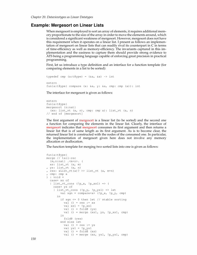
Chapter 20. Dataviewtypes as Linear Datatypes
Example: Mergesort on Linear ListsWhen mergesort is employed to sort an array of elements, it requires additional mem-ory proportionate to the size of the array in order to move the elements around, whichis considered a significant weakness of mergesort. However, mergesort does not havethis requirement when it operates on a linear list. I present as follows an implemen-tation of mergesort on linear lists that can readily rival its counterpart in C in termsof time-efficiency as well as memory-efficiency. The invariants captured in this im-plementation and the easiness to capture them should provide strong evidence toATS being a programming language capable of enforcing great precision in practicalprogramming.
First, let us introduce a type definition and an interface for a function template (forcomparing elements in a list to be sorted):
typedef cmp (a:t@ype) = (&a, &a) -> int
externfun{a:t@ype} compare (x: &a, y: &a, cmp: cmp (a)): int
The interface for mergesort is given as follows:
externfun{a:t@ype}mergesort {n:nat}(xs: list_vt (a, n), cmp: cmp a): list_vt (a, n)
// end of [mergesort]
The first argument of mergesort is a linear list (to be sorted) and the second onea function for comparing the elements in the linear list. Clearly, the interface ofmergesort indicates that mergesort consumes its first argument and then returns alinear list that is of same length as its first argument. As is to become clear, thereturned linear list is constructed with the nodes of the consumed one. In particular,the implementation of mergesort given here does not involve any memoryallocation or deallocation.
The function template for merging two sorted lists into one is given as follows:
fun{a:t@ype}merge // tail-rec{m,n:nat} .<m+n>. (xs: list_vt (a, m)
, ys: list_vt (a, n), res: &List_vt(a)? >> list_vt (a, m+n), cmp: cmp a) : void =case+ xs of| list_vt_cons (!p_x, !p_xs1) => (case+ ys of| list_vt_cons (!p_y, !p_ys1) => let
val sgn = compare<a> (!p_x, !p_y, cmp)inif sgn <= 0 then let // stable sortingval () = res := xsval xs1 = !p_xs1val () = fold@ (ys)val () = merge (xs1, ys, !p_xs1, cmp)
infold@ (res)
end else letval () = res := ysval ys1 = !p_ys1val () = fold@ (xs)val () = merge (xs, ys1, !p_ys1, cmp)
150

Chapter 20. Dataviewtypes as Linear Datatypes
infold@ (res)
end // end of [if]end (* end of [list_vt_cons] *)
| ~list_vt_nil () => (fold@ (xs); res := xs)) // end of [list_vt_cons]
| ~list_vt_nil () => (res := ys)// end of [merge]
Unlike the one given in a previous functional implementation, this implementationof merge is tail-recursive and thus is guaranteed to be translated into a loop in Cby the ATS compiler. This means that the concern of merge being unable to handlevery long lists (e.g., containg 1 million elements) due to potential stack overflow iscompletely eliminated.
The next function template is for splitting a given linear lists into two:
fun{a:t@ype}split {n,k:nat | k <= n} .<n-k>. (xs: &list_vt (a, n) >> list_vt (a, n-k), nk: int (n-k)
) : list_vt (a, k) =if nk > 0 then letval+ list_vt_cons (_, !p_xs1) = xsval res = split (!p_xs1, nk-1); val () = fold@ (xs)
inres
end else letval res = xs; val () = xs := list_vt_nil () in res
end // end of [if]// end of [split]
Note that the implementation of split is also tail-recursive.
The following function template msort takes a linear list, its length and a comparsionfunction, and it returns a sorted version of the given linear list:
fun{a:t@ype}msort {n:nat} .<n>. (xs: list_vt (a, n), n: int n, cmp: cmp(a)
) : list_vt (a, n) =if n >= 2 then letval n2 = n / 2val n3 = n - n2var xs = xs // a left-value for [xs]val ys = split {n,n/2} (xs(*cbr*), n3) // xs: call-by-refval xs = msort (xs, n3, cmp)val ys = msort (ys, n2, cmp)var res: List_vt (a)val () = merge (xs, ys, res(*cbr*), cmp) // xs: call-by-ref
inres
end else xs// end of [msort]
The second argument of msort is passed so that the length of the list being sorteddoes not have to be computed directly by traversing the list when each recursive callto msort is made.
Finally, mergesort can be implemented with a call to msort:
implement{a}mergesort (xs, cmp) = msort (xs, length (xs), cmp)
151

Chapter 20. Dataviewtypes as Linear Datatypes
Please find the entire code in this section plus some additional code for testing on-line1.
Linear Binary Search TreesA binary search tree with respect to a given ordering is a binary tree such that thevalue stored in each node inside the tree is greater than or equal to those stored inthe left child of the node and less than or equal to those stored in the right child of thenode. Binary search trees are a common data structure for implementing finite maps.
A family of binary trees are said to be balanced if there is a fixed constant C (for theentire family) such that the ratio between the length of a longest path and the lengthof a shortest path is bounded by C for every tree in the family. For instance, commonexamples of balanced binary trees include AVL trees and red-black trees. Finite mapsbased on balanced binary search trees support guaranteed log-time insertion anddeletion operations, that is, the time to complete such an operation is O(log(n)) in theworst case, where n is the size of the map.
In this section, I am to implement several basic operations on linear binary searchtrees, further illustrating some use of dataviewtypes. Let us first declare as follows adataviewtype bstree_vt for linear binary (search) trees:
dataviewtypebstree_vt(a:t@ype+, int) =| {n1,n2:nat}bstree_vt_cons (a, 1+n1+n2) of(bstree_vt (a, n1), a, bstree_vt (a, n2))
| bstree_vt_nil (a, 0) of ()// end of [bstree_vt]
Note that the integer index of bstree_vt captures the size information of a binary(search) tree. There are two constructors bstree_vt_cons and bstree_vt_nil associatedwith bstree_vt. It should be pointed out that the tree created by bstree_vt_nil is emptyand thus not a leaf, which on the other hand is a node whose left and right childrenare both empty. As a simple example, the following function template size computesthe size of a given tree:
fun{a:t@ype}size {n:nat} .<n>. (t: !bstree_vt (a, n)
) : int (n) =case+ t of| bstree_vt_cons (!p_tl, _, !p_tr) => let
val n = 1 + size (!p_tl) + size (!p_tr) in fold@ (t); nend // end of [bstree_vt_cons]
| bstree_vt_nil () => (fold@ (t); 0)// end of [size]
Assume that we have a binary search tree with repect to some ordering. If a predicateP on the elements stored in the tree possesses the property that P(x1) implies P(x2)whenever x1 is less than x2 (according to the ordering), then we can locate the leastelement in the tree that satisfies the predicate P by employing so-called binary searchas is demonstrated in the following implementation of search:
fun{a:t@ype}search {n:nat} .<n>. (t: !bstree_vt (a, n), P: (&a) -<cloref> bool
) : Option_vt (a) =case+ t of| bstree_vt_cons
152

Chapter 20. Dataviewtypes as Linear Datatypes
(!p_tl, !p_x, !p_tr) =>if P (!p_x) then letval res = search (!p_tl, P)val res = (case+ res of| ~None_vt () => Some_vt (!p_x) | _ => res
) : Option_vt (a)infold@ (t); res
end else letval res = search (!p_tr, P) in fold@ (t); res
end // end of [if]| bstree_vt_nil () => (fold@ (t); None_vt ())
// end of [search]
Clearly, if the argument t of search ranges over a family of balanced trees, then thetime-complexity of search is O(log(n)) (assuming that P is O(1)).
Let us next see an operation that inserts a given element into a binary search tree:
fun{a:t@ype}insert {n:nat} .<n>. (t: bstree_vt (a, n), x0: &a, cmp: cmp(a)
) : bstree_vt (a, n+1) =case+ t of| bstree_vt_cons
(!p_tl, !p_x, !p_tr) => letval sgn = compare<a> (x0, !p_x, cmp)
inif sgn <= 0 then letval () = !p_tl := insert (!p_tl, x0, cmp)
infold@ (t); t
end else letval () = !p_tr := insert (!p_tr, x0, cmp)
infold@ (t); t
end (* end of [if] *)end // end of [bstree_vt_cons]
| ~bstree_vt_nil () =>bstree_vt_cons (bstree_vt_nil, x0, bstree_vt_nil)
// end of [bstree_vt_nil]// end of [insert]
When inserting an element, the function template insert extends the given tree witha new leaf node containing the element, and this form of insertion is often referred toas leaf-insertion. There is another form of insertion often referred to as root-insertion,which always puts at the root position the new node containing the inserted element.The following function template insertRT is implemented to perform a standard root-insertion operation:
fun{a:t@ype}insertRT {n:nat} .<n>. (t: bstree_vt (a, n), x0: &a, cmp: cmp(a)
) : bstree_vt (a, n+1) =case+ t of| bstree_vt_cons
(!p_tl, !p_x, !p_tr) => letval sgn = compare<a> (x0, !p_x, cmp)
inif sgn <= 0 then letval tl = insertRT (!p_tl, x0, cmp)val+ bstree_vt_cons (_, !p_tll, !p_tlr) = tlval () = !p_tl := !p_tlrval () = fold@ (t)
153

Chapter 20. Dataviewtypes as Linear Datatypes
val () = !p_tlr := tinfold@ (tl); tl
end else letval tr = insertRT (!p_tr, x0, cmp)val+ bstree_vt_cons (!p_trl, _, !p_trr) = trval () = !p_tr := !p_trlval () = fold@ (t)val () = !p_trl := t
infold@ (tr); tr
endend // end of [bstree_vt_cons]
| ~bstree_vt_nil () =>bstree_vt_cons (bstree_vt_nil, x0, bstree_vt_nil)
// end of [bstree_vt_nil]// end of [insertRT]
The code immediately following the first recursive call to insertRT performs a righttree rotation. Let us use T(tl, x, tr) for a tree such that its root node contains the ele-ment x and its left and right children are tl and tr, respectively. Then a right rotationturns T(T(tll, xl, tlr), x, tr) into T(tll, xl, T(tlr, x, tr)). The code immediately followingthe second recursive call to insertRT performs a left tree rotation, which turns T(tl, x,T(trl, xr, trr)) into T(T(tl, x, tlr), xr, trr).
To further illustrate tree rotations, I present as follows two function templates lrotateand rrotate, which implement the left and right tree rotations, respectively:
fn{a:t@ype}lrotate{nl,nr:nat | nr > 0}{l_tl,l_x,l_tr:addr} (pf_tl: bstree_vt (a, nl) @ l_tl
, pf_x: a @ l_x, pf_tr: bstree_vt (a, nr) @ l_tr| t: bstree_vt_cons_unfold (l_tl, l_x, l_tr), p_tl: ptr l_tl, p_tr: ptr l_tr) : bstree_vt (a, 1+nl+nr) = letval tr = !p_trval+ bstree_vt_cons (!p_trl, _, !p_trr) = trval () = !p_tr := !p_trlval () = fold@ (t)val () = !p_trl := t
infold@ (tr); tr
end // end of [lrotate]
fn{a:t@ype}rrotate{nl,nr:nat | nl > 0}{l_tl,l_x,l_tr:addr} (pf_tl: bstree_vt (a, nl) @ l_tl
, pf_x: a @ l_x, pf_tr: bstree_vt (a, nr) @ l_tr| t: bstree_vt_cons_unfold (l_tl, l_x, l_tr), p_tl: ptr l_tl, p_tr: ptr l_tr) : bstree_vt (a, 1+nl+nr) = letval tl = !p_tlval+ bstree_vt_cons (!p_tll, x, !p_tlr) = tlval () = !p_tl := !p_tlrval () = fold@ (t)val () = !p_tlr := t
in
154
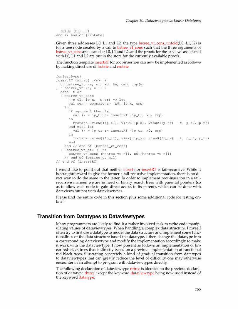
Chapter 20. Dataviewtypes as Linear Datatypes
fold@ (tl); tlend // end of [rrotate]
Given three addresses L0, L1 and L2, the type bstree_vt_cons_unfold(L0, L1, l2) isfor a tree node created by a call to bstree_vt_cons such that the three arguments ofbstree_vt_cons are located at L0, L1 and L2, and the proofs for the at-views associatedwith L0, L1 and L2 are put in the store for the currently available proofs.
The function template insertRT for root-insertion can now be implemented as followsby making direct use of lrotate and rrotate:
fun{a:t@ype}insertRT {n:nat} .<n>. (t: bstree_vt (a, n), x0: &a, cmp: cmp(a)
) : bstree_vt (a, n+1) =case+ t of| bstree_vt_cons
(!p_tl, !p_x, !p_tr) => letval sgn = compare<a> (x0, !p_x, cmp)
inif sgn <= 0 then letval () = !p_tl := insertRT (!p_tl, x0, cmp)
inrrotate (view@(!p_tl), view@(!p_x), view@(!p_tr) | t, p_tl, p_tr)
end else letval () = !p_tr := insertRT (!p_tr, x0, cmp)
inlrotate (view@(!p_tl), view@(!p_x), view@(!p_tr) | t, p_tl, p_tr)
endend // end of [bstree_vt_cons]
| ~bstree_vt_nil () =>bstree_vt_cons (bstree_vt_nil, x0, bstree_vt_nil)
// end of [bstree_vt_nil]// end of [insertRT]
I would like to point out that neither insert nor insertRT is tail-recursive. While itis straightforward to give the former a tail-recursive implementation, there is no di-rect way to do the same to the latter. In order to implement root-insertion in a tail-recursive manner, we are in need of binary search trees with parental pointers (soas to allow each node to gain direct access to its parent), which can be done withdataviews but not with dataviewtypes.
Please find the entire code in this section plus some additional code for testing on-line2.
Transition from Datatypes to DataviewtypesMany programmers are likely to find it a rather involved task to write code manip-ulating values of dataviewtypes. When handling a complex data structure, I myselfoften try to first use a datatype to model the data structure and implement some func-tionalities of the data structure based the datatype. I then change the datatype intoa corresponding dataviewtype and modify the implementation accordingly to makeit work with the dataviewtype. I now present as follows an implementation of lin-ear red-black trees that is directly based on a previous implementation of functionalred-black trees, illustrating concretely a kind of gradual transition from datatypesto dataviewtypes that can greatly reduce the level of difficulty one may otherwiseencounter in an attempt to program with dataviewtypes directly.
The following declaration of dataviewtype rbtree is identical to the previous declara-tion of datatype rbtree except the keyword dataviewtype being now used instead ofthe keyword datatype:
155
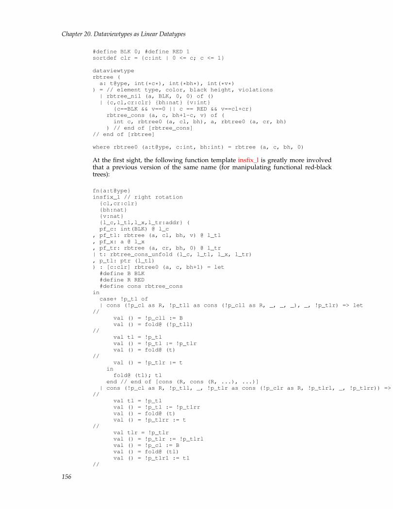
Chapter 20. Dataviewtypes as Linear Datatypes
#define BLK 0; #define RED 1sortdef clr = {c:int | 0 <= c; c <= 1}
dataviewtyperbtree (a: t@ype, int(*c*), int(*bh*), int(*v*)
) = // element type, color, black height, violations| rbtree_nil (a, BLK, 0, 0) of ()| {c,cl,cr:clr} {bh:nat} {v:int}
{c==BLK && v==0 || c == RED && v==cl+cr}rbtree_cons (a, c, bh+1-c, v) of (int c, rbtree0 (a, cl, bh), a, rbtree0 (a, cr, bh)
) // end of [rbtree_cons]// end of [rbtree]
where rbtree0 (a:t@ype, c:int, bh:int) = rbtree (a, c, bh, 0)
At the first sight, the following function template insfix_l is greatly more involvedthat a previous version of the same name (for manipulating functional red-blacktrees):
fn{a:t@ype}insfix_l // right rotation{cl,cr:clr}{bh:nat}{v:nat}{l_c,l_tl,l_x,l_tr:addr} (pf_c: int(BLK) @ l_c
, pf_tl: rbtree (a, cl, bh, v) @ l_tl, pf_x: a @ l_x, pf_tr: rbtree (a, cr, bh, 0) @ l_tr| t: rbtree_cons_unfold (l_c, l_tl, l_x, l_tr), p_tl: ptr (l_tl)) : [c:clr] rbtree0 (a, c, bh+1) = let#define B BLK#define R RED#define cons rbtree_cons
incase+ !p_tl of| cons (!p_cl as R, !p_tll as cons (!p_cll as R, _, _, _), _, !p_tlr) => let
//val () = !p_cll := Bval () = fold@ (!p_tll)
//val tl = !p_tlval () = !p_tl := !p_tlrval () = fold@ (t)
//val () = !p_tlr := t
infold@ (tl); tl
end // end of [cons (R, cons (R, ...), ...)]| cons (!p_cl as R, !p_tll, _, !p_tlr as cons (!p_clr as R, !p_tlrl, _, !p_tlrr)) => let
//val tl = !p_tlval () = !p_tl := !p_tlrrval () = fold@ (t)val () = !p_tlrr := t
//val tlr = !p_tlrval () = !p_tlr := !p_tlrlval () = !p_cl := Bval () = fold@ (tl)val () = !p_tlrl := tl
//
156

Chapter 20. Dataviewtypes as Linear Datatypes
infold@ (tlr); tlr
end // end of [cons (R, ..., cons (R, ...))]| _ =>> (fold@ (t); t)
end // end of [insfix_l]
However, I would like to point out that the interface for the above insfix_l is a directtranslation of the interface for the previous infix_l. In other words, the previouslycaptured relation between a tree being rotated and the one obtained from applyinginfix_l to it also holds in the setting of linear red-black trees. The very same can besaid about the following function template insfix_r, which is just a mirror image ofinsfix_l:
fn{a:t@ype}insfix_r // left rotation{cl,cr:clr}{bh:nat}{v:nat}{l_c,l_tl,l_x,l_tr:addr} (pf_c: int(BLK) @ l_c
, pf_tl: rbtree (a, cl, bh, 0) @ l_tl, pf_x: a @ l_x, pf_tr: rbtree (a, cr, bh, v) @ l_tr| t: rbtree_cons_unfold (l_c, l_tl, l_x, l_tr), p_tr: ptr (l_tr)) : [c:clr] rbtree0 (a, c, bh+1) = let#define B BLK#define R RED#define cons rbtree_cons
incase+ !p_tr of| cons (!p_cr as R, !p_trl, _, !p_trr as cons (!p_crr as R, _, _, _)) => let
//val () = !p_crr := Bval () = fold@ (!p_trr)
//val tr = !p_trval () = !p_tr := !p_trlval () = fold@ (t)
//val () = !p_trl := t
infold@ (tr); tr
end // end of [cons (R, ..., cons (R, ...))]| cons (!p_cr as R, !p_trl as cons (!p_crr as R, !p_trll, _, !p_trlr), _, !p_trr) => let
//val tr = !p_trval () = !p_tr := !p_trllval () = fold@ (t)val () = !p_trll := t
//val trl = !p_trlval () = !p_trl := !p_trlrval () = !p_cr := Bval () = fold@ (tr)val () = !p_trlr := tr
//infold@ (trl); trl
end // end of [cons (R, cons (R, ...), ...)]| _ =>> (fold@ (t); t)
end // end of [insfix_r]
157

Chapter 20. Dataviewtypes as Linear Datatypes
As can be expected, the following function template rbtree_insert is essentially a di-rect translation of the one of the same name for inserting an element into a functionalred-black tree:
externfun{a:t@ype}rbtree_insert{c:clr} {bh:nat} (t: rbtree0 (a, c, bh), x0: &a, cmp: cmp a
) : [bh1:nat] rbtree0 (a, BLK, bh1)
implement{a}rbtree_insert(t, x0, cmp) = let
//#define B BLK; #define R RED#define nil rbtree_nil; #define cons rbtree_cons//fun ins{c:clr} {bh:nat} .<bh,c>. (t: rbtree0 (a, c, bh), x0: &a
) :<cloref1> [cl:clr; v:nat | v <= c] rbtree (a, cl, bh, v) =case+ t of| cons (
!p_c, !p_tl, !p_x, !p_tr) => letval sgn = compare (x0, !p_x, cmp)
inif sgn < 0 then letval [cl,v:int] tl = ins (!p_tl, x0)val () = !p_tl := tl
inif !p_c = B theninsfix_l (view@(!p_c), view@(!p_tl), view@(!p_x), view@(!p_tr) | t, p_tl)
else letval () = !p_c := R in fold@ {a}{..}{..}{cl} (t); t
end // end of [if]end else if sgn > 0 then letval [cr,v:int] tr = ins (!p_tr, x0)val () = !p_tr := tr
inif !p_c = B theninsfix_r (view@(!p_c), view@(!p_tl), view@(!p_x), view@(!p_tr) | t, p_tr)
else letval () = !p_c := R in fold@ {a}{..}{..}{cr} (t); t
end // end of [if]end else (fold@ {a}{..}{..}{0} (t); t) // end of [if]
end // end of [cons]| ~nil () => cons {..}{..}{..}{0} (R, nil, x0, nil)
// end of [ins]val t = ins (t, x0)//in//case+ t of cons (!p_c as R, _, _, _) => (!p_c := B; fold@ (t); t) | _ =>> t//end // end of [rbtree_insert]
I literally implemented the above rbtree_insert by making a copy of theprevious implementation of rbtree_insert for functional red-black trees and thenproperly modifying it to make it pass typechecking. Although this processof copying-and-modifying is difficult to be described formally, it is fairlystraightforward to follow in practice as it is almost entirely guided by the errormessages received during typechecking.
158

Chapter 20. Dataviewtypes as Linear Datatypes
Please find the entire code in this section plus some additional code for testing on-line3. A challenging as well as rewarding exercise is for the reader to implement anoperation to delete an element from a given linear red-black tree.
Notes1. http://www.ats-lang.org/DOCUMENT/INTPROGINATS/CODE/CHAPTER_DATAVTYPES/mergesort.dats
2. http://www.ats-lang.org/DOCUMENT/INTPROGINATS/CODE/CHAPTER_DATAVTYPES/bstree_vt.dats
3. http://www.ats-lang.org/DOCUMENT/INTPROGINATS/CODE/CHAPTER_DATAVTYPES/rbtree.dats
159

Chapter 20. Dataviewtypes as Linear Datatypes
160

Chapter 21. Abstract Views and Viewtypes
I have so far given a presentation of views that solely focuses on at-views and theviews built on top of at-views. This is largely due to at-views being the form of mostwidely used views in practice and also being the first form of views supported inATS. However, other forms of views can be readily introduced into ATS abstractly.Even in a case where a view can be defined based on at-views (or other forms ofviews), one may still want to introduce it as an abstract view (accompanied withcertain proof functions for performing view changes). Often what the programmerreally needs is to figure out conceptually whether abstractly defined views and prooffunctions for manipulating them actually make sense. This is a bit like arguingwhether a function is computable: There is rarely a need, if at all, to actuallyencode the function as a Turing-machine to prove its being computable. IMHO,learning proper use of abstract views and abstract viewtypes is a necessary stepfor one to take in order to employ linear types effectively in practice to deal withresource-related programming issues.
Memory Allocation and DeallocationThe issue of memory allocation and deallocation is of paramount importance in sys-tems programming, where garabage collection (GC) at run-time is most likely forbid-den or only supported in a highly restricted manner. Handling memory managementsafely and efficiently is a long standing problem of great challenge in programming,and its novel solution in ATS is firmly rooted in the paradigm of programming withtheorem-proving (PwTP).
The following function malloc_gc is available in ATS for memory allocation:
fun malloc_gc (){n:nat} (n: size_t n):<> [l:agz] (freebyte_gc_v (n, l), b0ytes n @ l | ptr l)
// end of [malloc_gc]
The sort agz is a subset sort defined for addresses that are not null:
sortdef agz = {a:addr | a > null} // [gz] for great-than-zero
The type b0ytes(n) is a shorthand for @[byte?][n], which is for an array of nuninitialized bytes. Therefore, the at-view b0ytes(n)@l is the same as the array-viewarray_v(byte?, n, l). The view freebyte_gc_v(n, l) stands for a form of capabilityallowing that the n bytes located at the address l be freed (or reclaimed) by thefollowing function free_gc:
fun free_gc {n:nat} {l:addr}(pfgc: freebyte_gc_v (n, l), pfat: b0ytes n @ l | p: ptr l):<> void
// end of [free_gc]
Note that freebyte_gc_v is so far the first view we have encountered that is not builton top of any at-views.
In practice, it rather cumbersome to deal with bytes directly. Instead, the followingtwo functions are more convenient for allocating and deallocating arrays:
fun{a:viewt@ype}array_ptr_alloc {n:nat} (asz: size_t n):<> [l:agz] (free_gc_v (a, n, l), array_v (a?, n, l) | ptr l)
// end of [array_ptr_alloc]
fun array_ptr_free{a:viewt@ype} {n:int} {l:addr} (
161
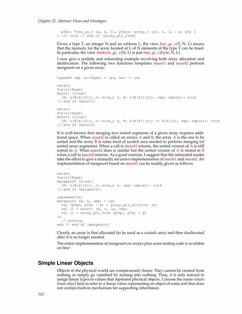
Chapter 21. Abstract Views and Viewtypes
pfgc: free_gc_v (a, n, l), pfarr: array_v (a?, n, l) | p: ptr l) :<> void // end of [array_ptr_free]
Given a type T, an integer N and an address L, the view free_gc_v(T, N, L) meansthat the memory for the array located at L of N elements of the type T can be freed.In particular, the view freebyte_gc_v(N, L) is just free_gc_v(byte, N, L).
I now give a realistic and interesting example involving both array allocation anddeallocation. The following two functions templates msort1 and msort2 performmergesort on a given array:
typedef cmp (a:t@ype) = (&a, &a) -> int
externfun{a:t@ype}msort1 {n:nat}(A: &(@[a][n]), n: size_t n, B: &(@[a?][n]), cmp: cmp(a)): void
// end of [msort1]
externfun{a:t@ype}msort2 {n:nat}(A: &(@[a][n]), n: size_t n, B: &(@[a?][n]) >> @[a][n], cmp: cmp(a)): void
// end of [msort2]
It is well-known that merging two sorted segments of a given array requires addi-tional space. When msort1 is called on arrays A and B, the array A is the one to besorted and the array B is some kind of scratch area needed to perform merging (ofsorted array segments). When a call to msort1 returns, the sorted version of A is stillsotred in A. What msort2 does is similar but the sorted version of A is stored in Bwhen a call to msort2 returns. As a good exercise, I suggest that the interested readertake the effort to give a mutually recursive implementation of msort1 and msort2. Animplementation of mergesort based on msort1 can be readily given as follows:
externfun{a:t@ype}mergesort {n:nat}(A: &(@[a][n]), n: size_t n, cmp: cmp(a)): void
// end of [mergesort]
implement{a}mergesort (A, n, cmp) = letval (pfgc, pfat | p) = array_ptr_alloc<a> (n)val () = msort1 (A, n, !p, cmp)val () = array_ptr_free (pfgc, pfat | p)
in// nothing
end // end of [mergesort]
Clearly, an array is first allocated (to be used as a scratch area) and then deallocatedafter it is no longer needed.
The entire implementation of mergesort on arrays plus some testing code is availableon-line1.
Simple Linear ObjectsObjects in the physical world are conspicuously linear: They cannot be created fromnothing or simply go vanished by turning into nothing. Thus, it is only natural toassign linear types to values that represent physical objects. I choose the name simplelinear object here to refer to a linear value representing an object of some sort that doesnot contain built-in mechanism for supporting inheritance.
162
Chapter 21. Abstract Views and Viewtypes
Let us first introduce a boxed abstract viewtype as follows for simple linear objects:
absviewtype sobjptr (a:viewt@ype+)
Given a viewtype VT, sobjptr(VT) is essentially meant for a pointer to some mem-ory location L where a value of the viewtype VT is stored. The following functiontemplate sobjptr_new and function sobjptr_free are for creating and destroying (i.e.,freeing) simple linear objects, respectively:
fun{a:viewt@ype} sobjptr_new (): sobjptr (a?)
fun sobjptr_free {a:viewt@ype} (x: sobjptr (a?)): void
The abstract viewtype sobjptr can be given the following definition:
assumesobjptr (a:viewt@ype) = [l:addr] @{atview= a @ l, gcview= free_gc_v (a?, l), ptr= ptr l
} // end of [sobjptr]
Subsequently, sobjptr_new and sobjptr_free can be implemented as follows:
implement{a}sobjptr_new () = letval (pfgc, pfat | p) = ptr_alloc<a> ()
in @{atview= pfat, gcview= pfgc, ptr= p
} end // end of [sobjptr_new]
implementsobjptr_free {a} (pobj) =ptr_free {a} (pobj.gcview, pobj.atview | pobj.ptr)
// end of [sobjptr_free]
Clearly, a simple object needs to be initialized before it is of any use. This can be doneby calling the following function sobjptr_init:
externfun sobjptr_init {a:viewt@ype}(pobj: !sobjptr (a?) >> sobjptr (a), f: (&a? >> a) -> void): void
// end of [sobjptr_init]
implementsobjptr_init(pobj, f) = letprval pfat = pobj.atviewval () = f !(pobj.ptr)prval () = pobj.atview := pfat
in// nothing
end // end of [sobjptr_init]
As a simple object may contain resources, it needs to be cleared out before it is al-lowed to be freed. This can be done by calling the following function sobjptr_clear:
externfun sobjptr_clear{a:viewt@ype} (x: !sobjptr (a) >> sobjptr (a?), f: (&a >> a?) -> void
) : void // end of [sobjptr_clear]
implement
163

Chapter 21. Abstract Views and Viewtypes
sobjptr_clear(pobj, f) = letprval pfat = pobj.atviewval () = f !(pobj.ptr)prval () = pobj.atview := pfat
in// nothing
end // end of [sobjptr_clear]
Note that each type T (of the sort t@ype) is a subtype of T?, implying that sobjptr(T)is a subtype of sobjptr(T?) (as sobjptr is co-variant). Therefore, sobjptr_free can becalled directly on a value of the type sobjptr(T) without need to call sobjptr_clear onthe value first.
Let us now see a concrete example of simple linear object. Suppose that a timer (thatis, stopwatch) is wanted to measure time (of some sort). Following is a natural inter-face for functions creating, destroying and manipulating timer objects:
absviewtype timerObj
fun timerObj_new (): timerObjfun timerObj_free (x: timerObj): voidfun timerObj_start (x: !timerObj): voidfun timerObj_finish (x: !timerObj): voidfun timerObj_pause (x: !timerObj): voidfun timerObj_resume (x: !timerObj): voidfun timerObj_get_ntick (x: !timerObj): uintfun timerObj_reset (x: !timerObj): void
The (flat) record type timer_struct is defined as follows to represent the state of atimer object:
typedeftimer_struct = @{started= bool // the timer has started
, running= bool // the timer is running// the tick number recorded
, ntick_beg= uint // when the timer was turned on the last time, ntick_acc= uint // the number of accumulated ticks} // end of [timer_struct]
The abstract viewtype timerObj can then be mapped to sobjptr(timer_struct):
assume timerObj = sobjptr (timer_struct)
The functions timerObj_new and timerObj_free can now be given the following im-plementation:
implementtimerObj_new () = lettypedef T = timer_structfn f (x: &T? >> T
) : void = {val () = x.started := falseval () = x.running := falseval () = x.ntick_beg := 0u // unsignedval () = x.ntick_acc := 0u // unsigned
} // end of [f]val pobj = sobjptr_new<T> ()
insobjptr_init {T} (pobj, f); pobj
end // end of [timerObj_new]
164
Chapter 21. Abstract Views and Viewtypes
implementtimerObj_free (pobj) = sobjptr_free {timer_struct} (pobj)
For brevity, I omit the code implementing the other functions on timer objects, whichthe interested reader can find on-line2 together with some additional testing code.
Example: Implementing an Array-Based Circular BufferArray-based circular buffers (of fixed sizes) are of common use in practice. For in-stance, in a typical client/server model, a circular buffer can be employed to holdrequests issued by multiple clients that are then processed by the server according tothe first-in-first-out (FIFO) policy. In a case where each request needs to be given apriority (chosen from a fixed set), a circular buffer can be created for each priority tohold requests of that priority.
I first declare a linear abstract type (that is, abstract viewtype) as follows for valuesrepresenting circular buffers:
absviewtype cbufObj (a:viewt@ype+, m:int, n: int)
Such values are considered simple linear objects (as inheritance is not an issue to bedealt with in this setting). Given a viewtype VT and two integers M and N, the view-type cbufObj(VT, M, N) is for a given buffer of maximal capacity M that currentlycontains N elements of the type VT.
Some properties on the parameters of cbufObj can be captured by introducing thefollowing proof function:
prfun cbufObj_param_lemma{a:viewt@ype} {m,n:int} (buf: !cbufObj (a, m, n)): [m>=n; n>=0] void
// end of [cbufObj_param_lemma]
The interface for the following two function templates indicates that they can becalled to compute the capacity and current size of a buffer:
fun{a:viewt@ype}cbufObj_get_cap{m,n:int} (buf: !cbufObj (a, m, n)
) : size_t (m) // end of [cbufObj_get_cap]
fun{a:viewt@ype}cbufObj_get_size{m,n:int} (buf: !cbufObj (a, m, n)
) : size_t (n) // end of [cbufObj_get_size]
While it is straightforward to use cbufObj_get_cap and cbufObj_get_size to tellwhether a buffer is currently empty or full, a direct approach is likely to be moreefficient. The following two function templates check for the emptiness and fullnessof a given circular buffer:
fun{a:viewt@ype}cbufObj_is_empty{m,n:int} (buf: !cbufObj (a, m, n)): bool (n==0)
fun{a:viewt@ype}cbufObj_is_full{m,n:int} (buf: !cbufObj (a, m, n)): bool (m==n)
165

Chapter 21. Abstract Views and Viewtypes
The functions for creating and destroying circular buffers are named cbufObj_newand cbufObj_free, respectively:
fun{a:viewt@ype}cbufObj_new {m:pos} (m: size_t m): cbufObj (a, m, 0)
fun cbufObj_free{a:viewt@ype} {m:int} (buf: cbufObj (a, m, 0)): void
// end of [cbufObj_free]
Note that a buffer can be freed only if it contains no elements as an element (of someviewtype) may contain resources. If elements in a buffer are of some (non-linear)type, then the following function can be called to clear out all the elements stored inthe buffer:
fun cbufObj_clear_type{a:t@ype} {m:int} (buf: !cbufObj (a, m, n) >> cbufObj (a, m, 0)
) : void // end of [cbufObj_clear_type]
The next two functions are for inserting/removing an element into/from a givenbuffer, which are probably the most frequently used operations on buffers:
fun{a:viewt@ype}cbufObj_insert{m,n:int | n < m} (buf: !cbufObj (a, m, n) >> cbufObj (a, m, n+1), x: a
) : void // end of [cbufObj_insert]
fun{a:viewt@ype}cbufObj_remove{m,n:int | n > 0} (buf: !cbufObj (a, m, n) >> cbufObj (a, m, n-1)
) : a // end of [cbufObj_remove]
Please find on-line the file circbuf.sats3 containing the entirety of the interface forfunctions creating, destroying and manipulating circular buffers.
There are many ways to implement the abstract type cbufObj and the functions de-clared in circbuf.sats4. In the on-line file circbuf.dats5, I give an implementation thatemploys four pointers p_beg, p_end, p_frst and p_last to represent a circular buffer:p_beg and p_end are the starting and finishing addresses of the underline array, re-spectively, and p_frst and p_last are the starting addresses of the occupied and un-occupied segments (in the array), respectively. What is special about this implemen-tation is its employing a style of programming that deliberately eschew the need forproof construction. While code written in this style is not guaranteed to be type-safe,the style can nonetheless be of great practical value in a setting where constructingformal proofs is deemed too great a requirement to be fully fulfilled. Anyone whotries to give a type-safe implementation for the functions declared in circbuf.sats6
should likely find some genuine appreciation for this point.
In the on-line file circbuf2.dats7, I give another implementation in which a circularbuffer is represented as a pointer p_beg plus three integers m, n and f: p_beg pointsto the starting location of the underline array, m is the size of the array (that is, thecapacity of the buffer), n is the number of elements currently stored in the buffer and fis the total number of elements that have so far been removed from the buffer. Again,proof construction is delibrately eschewed in this implementation.
From linearity to non-linearity
166

Chapter 21. Abstract Views and Viewtypes
Notes1. http://www.ats-lang.org/DOCUMENT/INTPROGINATS/CODE/CHAPTER_ABSVTYPES/mergesort.dats
2. http://www.ats-lang.org/DOCUMENT/INTPROGINATS/CODE/CHAPTER_ABSVTYPES/sobjptr.dats
3. http://www.ats-lang.org/DOCUMENT/INTPROGINATS/CODE/CHAPTER_ABSVTYPES/circbuf.sats
4. http://www.ats-lang.org/DOCUMENT/INTPROGINATS/CODE/CHAPTER_ABSVTYPES/circbuf.sats
5. http://www.ats-lang.org/DOCUMENT/INTPROGINATS/CODE/CHAPTER_ABSVTYPES/circbuf.dats
6. http://www.ats-lang.org/DOCUMENT/INTPROGINATS/CODE/CHAPTER_ABSVTYPES/circbuf.sats
7. http://www.ats-lang.org/DOCUMENT/INTPROGINATS/CODE/CHAPTER_ABSVTYPES/circbuf2.dats
167

Chapter 21. Abstract Views and Viewtypes
168
Chapter 22. Summary
169

Chapter 22. Summary
170