introduction to quantum geometry dynamics
DESCRIPTION
geometriaTRANSCRIPT
NOTE TO READER: a revised version is in the works and should be avaible in the coming
months. The new version will include new sections on celestial mechanics, a chapter on
bridging QGD properties and units with conventional measuring properties and units, and
further clarifications of key concepts. If you wish to be notified by email when it becomes
available, leave message at [email protected]
Introduction
To
Quantum-Geometry Dynamics
by
Daniel Burnstein
© 2010-2014
Space-Matter Interactions section revised November 20th 2014
1
Table of Contents
Hilbert’s 6th problem .................................................................................................. 6
Two Ways to do Science ............................................................................................. 8
Axiomatic Approach ........................................................................................................ 9
About the Source of Incompatibilities between Theories ............................................ 10
Quantum-Geometry Dynamics ..................................................................................... 11
Internal Consistency Necessary but Insufficient ........................................................... 12
Quantum-Geometrical Space ........................................................................................... 15
The nature of Space ...................................................................................................... 15
Theorem on the Emergence of Euclidian Space from Quantum-Geometrical Space
................................................................................................................................... 19
Propagation ................................................................................................................... 21
Interaction ..................................................................................................................... 21
Experimental verification .............................................................................................. 22
Principle of Conservation of Space and the Finite Universe ......................................... 23
Conservation of Preons(+) and their Intrinsic Properties of Mass and Energy .............. 23
Constancy of the Speed of Preons(+) ............................................................................. 24
Emerging Space and the Notion of Dimensions ............................................................ 26
Exclusion Extra Dimensions ...................................................................................... 26
Conservation of Space ................................................................................................... 26
The fundamental particle of matter; the preon(+) ............................................................ 29
Recapitulation and Implications .................................................................................... 30
Mechanisms of Formation of Particles ......................................................................... 30
Neutrino Formation .................................................................................................. 31
Photon Formation ..................................................................................................... 32
Mechanism of Electron or Positron Formation ........................................................ 33
Matter and Anti-matter (or the quantum-geometrical dynamics of electrons and
positrons and the electromagnetic effect. ............................................................... 36
Cosmological Implications of Structure of Neutrinos and Photons .............................. 36
Dark Matter Effect .................................................................................................... 36

2
The Preonic Field ....................................................................................................... 37
A Brief Discussion on the Concept of Time ....................................................................... 38
Clocks ............................................................................................................................. 39
Time Distance Equivalence............................................................................................ 39
On The Concept of Simultaneity ................................................................................... 39
Definition of an event: .................................................................................................. 39
Theorem of Instantaneity of Gravitational Interactions ............................................... 40
Definition of Simultaneity ............................................................................................. 40
Precedence .................................................................................................................... 41
Second Theorem of Simultaneity .................................................................................. 41
Principle of Strict Causality ............................................................................................ 41
Forces, Effects and Motion ............................................................................................... 42
The Gravity Effect .......................................................................................................... 42
Gravity effect between preons(+). ................................................................................. 43
Gravity effect between structures ................................................................................ 44
General Application of the QGD Gravity Equation ....................................................... 45
Mass .............................................................................................................................. 47
Energy ............................................................................................................................ 47
Momentum ................................................................................................................... 48
Calculating Direction of a Bound Preon(+) and Structures ............................................ 53
Why No Higgs Mechanism? .......................................................................................... 54
Calculating Direction of a Bound Preon(+) and Structures ............................................ 55
Heat, Temperature and Entropy ................................................................................... 56
Application to Exothermic Reactions within a System .................................. 57
Application to Cosmology ....................................................................................... 58
Preonic Fields and the Electromagnetic Effect ............................................................. 59
Preonic Polarization of a Region and the Effects of Attraction and Repulsion ........ 61
The Effect of Repulsion of Like-Charged Particles .................................................... 62
The Effect of Attraction of Like-Charged Particles .................................................... 63
3
Electromagnetic Effects at Non-Fundamental Scales ............................................... 64
Electromagnetic Effect of Neutron Stars .................................................................. 65
Reverse Electromagnetic Effects of Attraction and Repulsion ................................. 65
Dark Matter Effect ......................................................................................................... 66
QGD Prediction .............................................................................................................. 67
Dark Matter and the Pioneer and Mercury Anomalies ................................................ 67
Supporting Observations ............................................................................................... 67
The Structure of Nucleons and their Interactions ........................................................ 68
Example 1: proton-antiproton event ........................................................................ 69
Example 2: Neutron-proton event. ........................................................................... 70
The Structure of the Atomic Nucleus ............................................................................ 72
Gamma Decay ........................................................................................................... 75
Beta Decay ................................................................................................................ 76
Alpha Decay .............................................................................................................. 76
Formation of Nucleus and Nucleus Size ........................................................................ 79
Explanation of Free Neutron Instability and Proton Stability ....................................... 80
Size and Stability of Nucleons and Nuclei ..................................................................... 81
Energy, Momentum and the Laws of Motion ................................................................... 82
Speed Redefined ........................................................................................................... 82
QGD definition of Speed ............................................................................................... 83
Special cases: ............................................................................................................ 84
QGD Speed versus Classical Speed ................................................................................ 84
Space-Matter Interactions ................................................................................................ 86
Note about the Distinction between Mathematical and Physical Meanings ............... 87
Position, Speed and Trajectories ................................................................................... 87
Application at the Newtonian Scale .............................................................................. 89
Experimental Prediction ........................................................................................... 90
Laws of Motion and Optics ............................................................................................... 91
First Law of Motion ....................................................................................................... 91

4
Second Law of Motion................................................................................................... 91
Optics ............................................................................................................................. 92
Refraction of Light ......................................................................................................... 97
Reflection and the Photoelectric Effect ...................................................................... 100
QGD Optical Transistor ........................................................................................... 101
Optics and Quantum Thermodynamics ...................................................................... 101
The Effect of Photon/Electron Interaction on the Motion of Electrons ..................... 103
Atoms Composed of Several Nucleons and Electrons ............................................ 107
Proton-Particle Interactions .................................................................................... 108
Nucleon and Nucleus Equilibriums ......................................................................... 108
Quantum Thermodynamics .................................................................................... 109
Modes of Photon Absorption and Emission ........................................................... 112
The Casimir Effect ................................................................................................... 113
Redshift Effect and Cosmological Implications ........................................................... 114
On Measuring the Immeasurable ............................................................................... 116
Other Immeasurables and the Experimental Method ................................................ 118
Gravity and the Speed of Light .................................................................................... 119
Addendum: About the Michelson-Morley Attempt at Measuring the Immeasurable
..................................................................................................................................... 120
Conclusion ............................................................................................................... 120
Collision Physics at Our Scale and the Mechanics of Momentum Transfer ................... 122
Baseball Physics ........................................................................................................... 122
Newton’s Cradle .......................................................................................................... 126
States of Gravitationally Interacting Bodies ................................................................... 131
Introduction to QGD Cosmology..................................................................................... 133
The Material and Spatial Dimensions of the Universe................................................ 134
Principles of QGD Cosmology ...................................................................................... 134
Law of Conservation: ........................................................................................... 135
Conservation of Space ............................................................................................ 135
Particle Formation and Strict Causality .................................................................. 136
5
The Cosmic Microwave Background Radiation ...................................................... 137
Cosmic Neutrino Background ................................................................................. 137
Small Structure Formation ...................................................................................... 137
Large Structures ...................................................................................................... 137
Black Holes and Black Holes Physics ........................................................................... 137
Angle between the Rotation Axis and the Magnetic Axis ...................................... 138
The Inner Structure of Black Holes ......................................................................... 138
Neutron Stars, Pulsars and Other Supermassive Structures .................................. 140
Cosmological Consequences ................................................................................... 141
Locally Condensing Universe ....................................................................................... 141
Consequences for Particle Physics .......................................................................... 143
The Preonic Universe .................................................................................................. 144
Mapping the Universe ................................................................................................. 146
Emission Spectrum of Atoms .................................................................................. 146
QGD’s Interpretation of the Redshift and Blueshift Effects ................................... 148
Gravitational Telescopy .......................................................................................... 149
Mass Change of Photons over Distance ................................................................. 149
Cosmological Implications ...................................................................................... 149
Application to Unsolved Problems ................................................................................. 150
Addendum: Principles, Axioms and Theorems of QGD .................................................. 151
Principle of Strict Causality .......................................................................................... 151
Conservation Law and the Fundamentality Theorem................................................. 151
Axioms and Theorems of Quantum-Geometry Dynamics .......................................... 151

6
I wish merely to point out the lack of firm foundation for assigning any physical reality to the
conventional continuum concept. My own view is that ultimately physical laws should find their
most natural expression in terms of essentially combinatorial principles, that is to say, in terms of
finite processes such as counting or other basically simple manipulative procedures. Thus, in
accordance with such a view, should emerge some form of discrete or combinatorial space-time.
Roger Penrose, On the Nature of Quantum-Geometry
Hilbert’s 6th problem
In 1900, the famous mathematician David Hilbert introduced a list of 24 great problems
in mathematics. The list of problems addressed a number of important issues in
mathematics; many of which have remained to this day unresolved. Hilbert’s 6th
problem, which has become central to physics, reads as follow:
To treat in the same manner, by means of axioms, those physical sciences in which
already today mathematics plays an important part; in the first rank are the theory of
probabilities and mechanics.
Though it was not a consideration at the time of its equationtion, Hilbert’s 6th problem is
really about creating a grand unified theory of physics.
The approach suggested by Hilbert’s problem was to create a finite and complete set of
axioms from which all the governing laws of the Universe could be derived. He
suggested that a physics theory be an axiomatic system; that is, a theory that is founded
on axioms from which all physics can be deduced from or reduced to.
An axiom, as most of you know, is a fundamental assumption or proposition about a
domain. What this means is that it can’t be reduced, derived or deduced from any other
propositions. In other words, an axiom cannot be mathematically proven.
All propositions, theorems, corollaries, that is, anything that can be said of a particular
domain can be deduced from the set of axioms of that particular domain.
In physics, axioms are understood as representing fundamental properties or
components of reality. My understanding of Hilbert’s 6th problem is that a set of axioms
about physical reality that is complete be created. That is, all observations, any and all
phenomenon could be deduced from the set of axioms. The set of axioms and laws,
explanations and predictions deduced from it would form an axiomatic system or
axiomatic theory which would axiomatize the whole of physics.
It seems evident that the purpose of physics is to identify the fundamental properties or
components of reality and to use them to develop theories that can explain
7
observations of physical phenomena. What is less evident is how to determine when the
propositions chosen by physicists to be the basis of a theory are really axioms.
While in mathematics one can arbitrarily chose any consistent set of axioms as a basis of
an axiomatic system, the axioms in a physics theory must represent fundamental
aspects of reality. This raises the essential question: What constitutes a fundamental
aspect of reality?
As we will see in this book, quantum-geometry dynamics proposes that reality obeys a
principle of strict causality. From the principle of strict causality, it follows that an aspect
of reality is fundamental if it is absolutely invariable. That is, regardless of interactions
or transformations it is subjected to, a fundamental aspect of reality remains
unaffected.
Now that we established what we mean by a fundamental aspect of reality, two
presuppositions need to be accepted in order to answer Hilbert’s 6th problem. First, we
must assume that the Universe is made of fundamental objects having properties which
determine a consistent set of fundamental laws. Second, that it can be represented by a
complete and consistent axiomatic system. That is, the Universe has a finite set of
fundamental components which obey a finite set of fundamental laws. These two
presuppositions are essential for the construction of any true axiomatic system.
In addition to the two presuppositions, there is also the question of the minimum axiom
set necessary to form a complete and consistent axiomatic theory.
To determine that value, we need to remember that the number of constructs that can
be built from a finite set of fundamental objects is always greater than the number of
objects in the set.
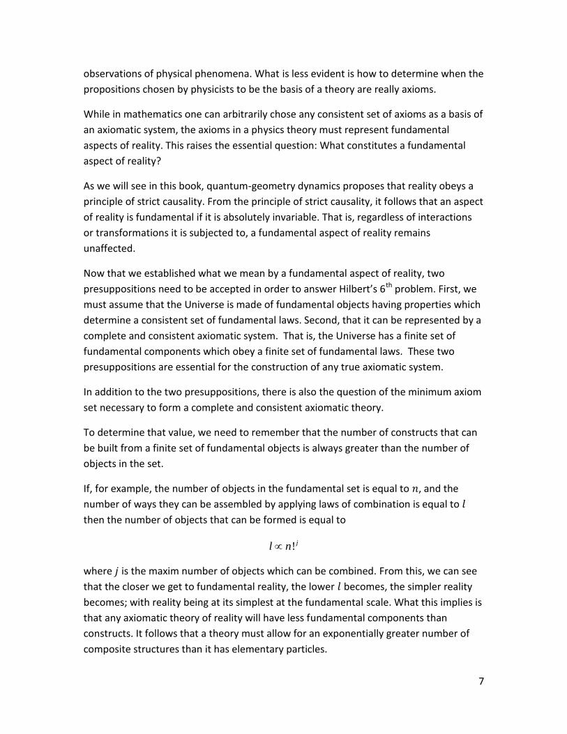
If, for example, the number of objects in the fundamental set is equal to 𝑛, and the
number of ways they can be assembled by applying laws of combination is equal to 𝑙
then the number of objects that can be formed is equal to
! jl n
where 𝑗 is the maxim number of objects which can be combined. From this, we can see
that the closer we get to fundamental reality, the lower 𝑙 becomes, the simpler reality
becomes; with reality being at its simplest at the fundamental scale. What this implies is
that any axiomatic theory of reality will have less fundamental components than
constructs. It follows that a theory must allow for an exponentially greater number of
composite structures than it has elementary particles.

8
In plain language, reality at the fundamental scale is simpler, not more complex.
So what is the smallest possible set of axioms an axiomatic theory of fundamental
physics can have?
Before answering this question, quantum-geometry dynamics first asks: What does
everything in the Universe have in common? What does every single theory of physical
reality ever thought of have in common?
The answer: space and matter. Space and matter are aspects of reality shared by
everything, all phenomena, all events in the Universe. So any axiomatic theory of
physical reality must minimally account for space and matter. So, the smallest number
of axioms an axiomatic theory of physics can have is two; a space axiom and a matter
axiom. Quantum-geometry dynamics, the theory discussed in the book, is founded on
the following two axioms.
Space made of discrete particles, preons
, and is dimensionalized by the repulsion
force acting between them.
Matter is made of fundamental kinetic particles, preons
, which form structure as a
result of the attractive force acting between them (p-gravity).
Two Ways to do Science
From an axiomatic standpoint, there are two only two ways to do science. The first aims
to extend, expand and deepen an existing theory; which is what the overwhelming
majority of theorists do. This approach assumes that the theory is fundamentally
correct, that is, the axiom set it is based is on are thought to correspond to fundamental
aspect of reality.
The second way of doing physics is to start with an entirely new axiom set and derives
from it a theory. Distinct axiom sets will lead to distinct theories which, even if they are
mutually exclusive may still describe and explain phenomena in ways that are consistent
with observations. There can be a multiplicity of such correct theories if the axioms are
made to correspond to observed aspects of reality that are not fundamental but
emerging. For instance, theories have been built where one axiom states that the
fundamental component of matter is the atom. Such theories, though it make describe
very well some phenomena at the molecular scale will fail in explaining of number of
phenomenon at smaller scales. In the strict sense, premises based on emergent aspect
of reality are not axioms in the physical sense. They can better be understood as
theorems. And as mathematical theorems in mathematics can explain the behavior of
mathematical objects belonging to a certain class but cannot be generalized to others,
9
physical theorems can explain the behavior of class of objects belong to a certain scale,
their explanations cannot be extended to others scales or even to objects of other
classes of objects in the same scale.
Axiom sets are not inherently wrong or right. By definition, since axioms are the starting
point, they cannot be reduced or broken down. Hence, as such, we cannot directly
prove whether they correspond to fundamental aspects of reality. However, if the
models that emerge from an axiom set explain and describe reality and, most
importantly, allows predictions that can be tested, then confirmation of the predictions
become evidence supporting the validity of the axiom set.
Axiomatic Approach It can scarcely be denied that the supreme goal of all theory is to make the irreducible
basic elements as simple and as few as possible without having to surrender the
adequate representation of a single datum of experience.
Albert Einstein
The dominant approach in science (and a hugely successful one for that matter) is the
empirical approach. That is, the approach by which science accumulates data from
which it extracts relationships and assumptions that better our understanding of the
Universe.
The empirical approach is an essential part of what one which we might call
deconstructive. By that I mean that we take pieces or segments of reality from which,
through experiments and observations, we extract data from which we hope to deduce
the governing laws of the Universe. But though the deconstructive approach works well
with observable phenomena, it has so far failed to provide us with a consistent
understanding of fundamental reality.
Of course, when a theory is equationted that is in accord with a data set, it must be
tested against other data sets for which it makes predictions. And if the data disagrees
with predictions, the theory may be adjusted so as to make it consistent with the data.
Then the theory is tested against a new or expanded data set to see if it holds. If it
doesn’t, the trial and error process may be repeated so the theory becomes applicable
to an increasingly wider domain of reality.
The amount of data accumulated from experiments and observations is astronomical,
but we have yet to find the key to decipher it and unlock the fundamental laws
governing the Universe.
10
Also, data is subject to countless interpretations and the number of mutually exclusive
models and theories increases as a function of the quantity of accumulated data.
About the Source of Incompatibilities between Theories
Reality can be thought as an axiomatic system in which fundamental aspects correspond
to axioms and non-fundamental aspects correspond to theorems.
The empirical method is essentially a method by which we try to deduce the axiom set
of reality, the fundamental components and forces, from theorems (non-fundamental
interactions). There lies the problem. Even though reality is a complete and consistent
system, the laws extracted from observations at different scales of reality and which
form the basis of physics theories do not together form a complete and consistent
axiomatic system.
The predictions of current theories may agree with observations at the scale from which
their premises were extracted, but they fail, often catastrophically, when it comes to
making predictions at different scales of reality.
This may indicate that current theories are not axiomatic; they are not based on true
physical axioms, that is; the founding propositions of the theories do not correspond to
fundamental aspects of reality. If they were, then the axioms of distinct theories could
be merged into consistent axiomatic sets. There would be no incompatibilities.
Also, if theories were axiomatic systems in the way we describe here, their axioms,
would be similar or complementary. Physical axioms can never be in contradiction.
This raises important questions in regards to the empirical method and its ability to
extract physical axioms from theorems it deduces from observations. Even theories
which are based on the observations of phenomena at the microscopic scale have failed
to produce physical axioms (if they had, they would explain interactions at larger scales
as well) suggesting that there is an important distinction to be made between
microscopic and fundamental. There is nothing that allows us to infer that what the
microscopic scale is the fundamental scale or that what we observe at the microscopic
scale is fundamental. It may very well be, as QGD suggests, that everything we hold as
fundamental, the particles, the forces, etc., are not. So we ended up with theorems
which can be applied successfully to the scale they were extracted from, but not to
others scales.
Also, theories founded on theorems rather than axioms cannot be unified. It follows
that the grand unification of the reigning theories which has been the dream of
generation of physicists is mathematically impossible. A theory of everything cannot

11
result from the unification of the standard model and relativity, for instance, them being
based on mutually exclusive axiom sets. This is why one of the biggest concerns, when
working on QGD, was to abide to the initial axiomatic set rigorously so as to avoid
coercing the theory into agreeing with any other theory. In other words, I wanted to let
the theory develop in a manner consistent with its axiom set. So even though, for
example, Newton’s law of universal gravity and 𝐸 = 𝑚𝑐 have been derived from QGD,
they naturally followed from its axiom set.
But what if fundamental reality is unobservable? Would science ultimately fail to
provide an axiomatic theory of the Universe, a theory of everything? Not necessarily
(see article On Measuring the Immeasurable).
We will show that fundamental reality is unobservable, but that does not imply that an
axiomatic theory is impossible. It may be possible to devise a complete and consistent
set of axioms to which interactions at all scales of reality can be reduced to. This means
that even if the fundamental scale of reality remains unobservable, an axiomatic theory
would make precise predictions at scales that are.
Quantum-Geometry Dynamics
Quantum-geometry dynamics, the theory discussed in this book, favours a constructive
approach instead of the deconstructive approach generally taken by science. What that
means is that quantum-geometry dynamics is a theory developed from a small set of
axioms.
If, as we assume, the axiom set of QGD is complete, then the theory derived from will
hold true for all physical phenomenon and all scales of reality from the fundamental to
the cosmological.
Absolute and Non-Arbitrary Measuring System
One aspect of quantum-geometry dynamics which may somewhat be disorienting at
first is that it considers all aspect of fundamental reality to be discrete. There is a
fundamental unit of distance, which cannot be subdivided in smaller units, for example,
so all distances are integer values of the fundamental unit of distance. In the same way,
energy, mass, interactions, momentum are all expressed using the fundamental discrete
units. All values are absolute and exact using discrete fundamental units.

12
Internal Consistency Necessary but Insufficient
Any theory that is rigorously developed from a given consistent set of axioms will itself
be internally consistent. That said, any number of theories can created that will be
internally consistent. But to be a valid physics theory, not only does it need to be
internally consistent, it must be consistent with physical reality. Because of that, three
things are required of a physics theory.
That it describes physical phenomena and
that is explains physical phenomena and
that is makes testable predictions that are original to it.
A number of now prevalent theories do not fulfill the above requirements. The Standard
Model, for one, describes the behavior of subatomic particles but fails to provide
explanations and makes probabilistic predictions which, it can be argued aren’t really
any more predictions than predicting the probability that an ace may be pulled out at
random from a deck of cards.
General Relativity, on the other hand, does better in that it describes gravity and makes
deterministic predictions, but it does not explain the cause of gravity.
Some theories are what we call effective theories. These theories describe physical
phenomena without providing any mechanisms by which they occur. Some of the
dominant theories are effective theories. The standard model of particle physics, for
instance is such a theory. But though it can make probabilistic predictions, it does not
explain the reasons why particles behave the way they do. Because it doesn’t provide
any mechanisms from which to make the predictions, it cannot be deterministic and
must instead be probabilistic. According to those theories physical phenomena happen
because it has been observed that under certain conditions, there is a probability that
they will. This is not an explanation. So the standard model of particle physics, since it
doesn’t explain, is an effective theory; which is another way of saying that the theory is
incomplete.
A physics theory is required to describe, explain and predict. Nothing less, nothing more.
The politics surrounding the physics “industry” (see Lee Smolin’s The Trouble with
Physics) and other sociological factors will determine whether a theory will be accepted
or rejected, or come into favour, even rise to become dominant only to fall out of favour
when new experimental results come up. I will try here to stir away from the politics of
physics and write about what makes a theory scientifically successful (as opposed to
sociologically successful).
13
A physics theory must describe a certain class of phenomena, explain them satisfactorily
and make predictions which can be experimentally or observationally confirmed.
I received an email a few years ago from a German physicist who was quite disturbed by
the fact that, as he puts it, quantum-geometry dynamics goes against much of the
dominant theories of physics. Not only does it not fit with dominant theories, it
approaches the problem of developing a fundamental theory of reality axiomatically
rather than empirically.
He was right of course. QGD does question a number of notions and concepts which we
have come to accept (often unconsciously) as absolute truths. For example, all dominant
theories are based on the axiom of continuity of space.
QGD is founded on the axiom of discreteness of space. Not only does QGD consider
space to be discrete, it proposes that space be the result of the interactions between
preons
; one of only two types fundamental particles the theory admits. Thus space is
dimensionalized by preons
.
QGD can be understood as a physics theory of quantum-geometrical space that implies
that the structure of space determines the structure of matter and not the reverse.
QGD explains that the constancy of the speed of light is a direct consequence of the
quantum-geometrical structure of space and shows that time is a pure relational
concept having no physical reality. This is in disagreement with special relativity which
imply that time is real.
QGD also considers that mass is a fundamental property of matter and proposes that all
matter is made of preons
. So all the particles which physics considers fundamental
are, according to the QGD model, composite particles. Even photons, are shown to be
composite particles made of preons
. Thus QGD is in opposition with the standard
model.
Finally, since a direct implication of space being quantum-geometrical is that the
Universe evolved from an isotropic state rather than a singularity, it is also doesn’t sit
well with the Big Bang theory.
Given the examples above, I must concede that QGD disagrees with the dominant
theories in physics. That said, agreeing with any theory, however successful it may be, is
not a requirement. A theory must describe, explain and predict. In other words, a theory
is only required to agree with reality. That said, the only entity that needs to be
14
convinced of the validity of a theory is Nature herself. Regrettably, many feel that not
only doesn’t she need to be convinced, she doesn’t even have a say in the matter.
When working on QGD, one of my biggest concern was to follow the initial axiomatic set
rigorously so as to avoid coercing the theory into agreeing with any other theory. In
other words, I wanted to let the theory develop in a manner consistent with its axiom
set. Also as important as avoiding coercing the QGD to agree with another theory, it was
essential to avoid contriving it to agree with experimental and observational data (which
is another mistake science makes), but instead only compare explanations and
predictions which have first been rigorously derived from the axiom set.
All a theory of physics is required to do is describe, explain and predict the behaviour of
physical systems. So the only question that matters when it comes to quantum-
geometry dynamics is: Does it agree with reality?
QGD, which follows from the axiom of discreteness of space, forces us to rethink some
assumptions we have come to make about physical reality; even basic notions such as
that of mass, energy, momentum come into question. Choosing the axiom of
discreteness of space instead of that of continuity of space has profound consequences
for all of physics. Virtually all physics theory assume that space is continuous, so it’s not
surprising that a physics theory based on discreteness of space provides descriptions of
physical systems that are radically different from continuum based theories.
Letting go of foundational concepts is difficult, especially for professional physicists. This
is understandable and even more difficult when these foundational concepts are the
basis of successful theories reinforced by decades of study, research and models which
are often supported by experimental data.
It is also understandable that physicists will evaluate new ideas from within the
framework of the theories they use to make sense of reality. Yet, as I insisted earlier, a
new theory doesn’t need the validation of other even well established and tested
theories any more than nature requires science to exist.
No theory can be validated from within the framework of another theory when they are
based on mutually exclusive axiom sets. Theories issued from mutually exclusive axiom
sets are mathematically bound to disagree. So my advice to all readers is to study QGD
for itself and outside the framework of any other theory and to check it for internal
consistency and most importantly for consistency with physical reality. Thus the validity
of a theory can only be determined by observation and experimentation.
15
Quantum-Geometrical Space Let me say at the outset that I am not happy with this state of affairs in physical theory.
The mathematical continuum has always seemed to me to contain many features which
are really very foreign to physics. […] If one is to accept the physical reality of the
continuum, then one must accept that there are as many points in a volume of diameter
1013 cm or 1033 cm or 101000 cm as there are in the entire universe. Indeed, one must
accept the existence of more points than there are rational numbers between any two
points in space no matter how close together they may be. (And we have seen that
quantum theory cannot really eliminate this problem, since it brings in its own complex
continuum.)
Roger Penrose, One the Nature of Quantum-Geometry
The nature of Space
I consider it quite possible that physics cannot be based on the field concept, i. e., on
continuous structures. In that case nothing remains of my entire castle in the air
gravitation theory included, [and of] the rest of modern physics. - Einstein in a 1954
letter to Besso.
What Einstein might have been referring to is that special relativity and general
relativity require that space be continuous. The axiom of continuity of space is implied
by special relativity as well as most current physics theory.
Einstein understood that if the unstated continuity axiom turned out to be false, his
theory and all theories which require it be true would also fall apart. That is not the
case. The dominant theories successfully explained and in some case predicted
experimental observations. That said, even the most successful and dominant theories,
which work only at a particular scale, ultimately fail to appropriately describe or predict
phenomena at others scales of physical reality. What all the dominant theories have in
common is the axiom of continuity of space. QGD differs as it is based on the axiom of
discreteness of space. We will explore some of the consequences of space being
discrete.
Quantum-geometry dynamics postulates that space is discrete. Specifically, that
quantum-geometric space is generated by fundamental particles we call preons
,
symbol ( ) p , and the force between any two
preons
is the fundamental unit of n-
gravity force g . According to QGD, spatial dimensions are emergent properties of
preons
, hence space is not fundamental.

16
It is important here to remind the reader that what exists between two preons
is the
n-gravity field. There is no space in the geometrical sense between them. The force of
the field between any two preons
, anywhere in the Universe, is equal to
g .
The figure above is a two dimensional representation of quantum-geometrical space.
The green circle represents a preon
arbitrarily chosen as origin and the blue circles
represent preons
which are all at one unit of distance from it. As we can see, distance
in quantum-geometrical space at the fundamental scale is very different than Euclidian
distance (though we will show below that Euclidian geometry emerges from quantum-
geometrical space at larger scales).
Quantum-geometric space is physical and not purely mathematical or geometrical.
Because of that, in order to distinguish it from quantum-geometric space, we will refer
to space in the classical sense of the term as Euclidian space.
Quantum-geometric space is very different from metric space. A consequence of this is
that the distance between any two preons
in quantum-geometric space is be very
different from the measure of the distance using Euclidian space; the distance between
17
two points or preons
being equal to the number of leaps a
preon
would need to
make to move from one to the other.
In order to understand quantum-geometric space, one must put aside the notion of
continuous and infinite space. Quantum-geometric space is created by the n-gravity
interactions between preons
. What that means is that
preons
does not propagate
through space, they are space. Since preons
are fundamental and since QGD is
founded on the principle of strict causality, then the n-gravity field between preons
has always existed and as such may be understood as instantaneous. N-gravity (or p-
gravity for that matter) does no propagate. It just exists.
The following figure shows another examples of how the distance between to preons
is calculated. So although the Euclidian distance between the green preon
and any
one of the blue preons
are nearly equal, the quantum-geometrical distances between
the same varies greatly.
Since the quantum-geometrical distances do not correspond to the Euclidian distances,
the theorems of geometry do not hold. Trying to apply Pythagoras’s theorem to the
triangle which in the figure below is defined by the blue, the red and the orange lines,
we see that 2 2 2a b c .

18
Also interesting the above figure is that if a is the orange side, b the red side and c the
blue side (what would in Euclidian geometry be the hypotenuse, then a c b . That is,
the shortest distance between two preons
is not necessarily the straight line.
But we evidently live on a scale where Pythagoras’s theorem holds, so how does
Euclidian geometry emerge from quantum-geometrical space. The figure below shows
the preons
through which two objects of similar size go through but in different
directions.

19
Here, if we consider that the area in the blue rectangles is made of all the preons
through which the object goes through, we see that as we move to larger scales, the
number preons
contained in the green rectangle approaches the number of
preons
in the blue rectangle, so that if the distance from a to b or from a to b is
defined by the number of preons
contained in the respective rectangles divided by
the width of the path, we find that a b a b .
Theorem on the Emergence of Euclidian Space from Quantum-Geometrical Space
Given n bounded preons
, moving in parallel trajectories at distance of 1d
between them, and given that the average distance d is equal to 1
n
i
i
d
n
, then as n
approaches a minimum value M , lim Eun M
d d
, where Eud is the Euclidian distance
travelled by each of the preons
.
What that theorem means is that beyond a certain scale, the Euclidian distance
between two points provides a good approximation of the quantum-geometrical

20
distance, but that below that scale, the closer we move towards the fundamental scale,
the greater the discrepancies between Euclidian and quantum-geometrical
measurements of distance.
In the figure above, if 1n , 2n and 3n are respectively the number of parallel trajectories
that sweep the squares a , b and c , for 1 3n M , then
1
1
1
n
i
ì
d
an
,
2
1
2
n
i
ì
d
bn
and
3
1
3
n
i
ì
d
cn
so that 2 2 2a b c . Hence, given the quantum-geometrical length of the
sides of any two of the three squares above, Pythagoras’s theorem can be used to
calculate an approximation of a the length of the side of the third. Also, the greater the
values of 1n , 2n and 3n the closer the approximation will be to the actual unknown
length. That is 1
2
2
2 2 2limnnn
a b c
.

21
Propagation
Simply put, propagation implies motion; the displacement of matter ( preons
) through
quantum-geometric space. A preon
, which is the fundamental particle of matter,
moves by leaps from preon
to
preon
. Therefore, the displacement of a preon
is
equal to the number of leaps it makes.
Also, the speed of preons
is speed limited by the structure of quantum-geometric
space. That is, a preon
must move by a succession of single leaps between adjacent
preons
along its trajectory. So the preonic leap, or leap, must be the smallest unit of
motion. The speed at which this leap occurs will be shown to be equal to the speed of
light (we will see later that QGD’s definition of speed differs fundamentally from its
classical definition).
Note that from the description of gravitational interaction which we will introduce later
we can deduce the following.
Theorem of Adjacency
That is, two preons
a and b are adjacent if ; 1G a b .
We will discuss this further in the present and following chapters, but for now, let’s just
remember that, according to quantum-geometry dynamics, the constancy of the speed
of light is a consequence of the structure of space.
Interaction
Interactions, gravity for example, do not require the displacement of matter. So unlike
propagations, interactions are not mediated by quantum-geometric space ( preons
).
We already explained that quantum-geometric space is generated by the interaction
between preons
; the n-gravity field between them. N-gravity does not propagate
through quantum-geometric space, it generates it. It follows that n-gravity is
instantaneous. P-gravity, the force acting between preons
is similarly instantaneous
and, as we will see later, so must be gravity; the resultant effects of n-gravity and p-
gravity.
That interactions are instantaneous also implies that fluctuations in the interactions are
also instantaneous.
Thus, the gravitational interaction between two objects changes instantaneously as a
function of mass and distance. The changes in mass themselves are not instantaneous
22
as such –they require absorption or emission of particles, both of which imply
propagations –but the resulting fluctuation in the gravitational interaction is.
The implication for experimental physics is that gravitational interactions and their
fluctuations can be measured instantly. But since there is no propagation, there is no
such thing as gravity waves. Since gravity is an interaction, the concept of speed of
propagation is inapplicable.
Experimental verification
For QGD to be a valid theory, the instantaneity of gravity must be experimentally
verifiable. A simple experiment:
QGD proposes that all objects in the Universe are gravitationally interacting with only
the magnitude in the interactions varying in accordance to the gravitational interaction
equation (this will be introduced in the chapter titled Forces, Effects and Motion).
Changes in the mass of two objects or changes in distance will instantly affect the
magnitude of the gravitational interaction between them. Instantaneity implies that
there is no propagation and that gravity has no speed. In other words, gravitational
interactions simply exist. Since gravity has no speed, QGD predicts that any experiment
designed to measure the speed of propagation of gravity is bound to fail.
But though we can’t measure instantaneity, we can design an experiment which takes
advantage of the fact that we can measure variations in the gravitational interaction to
prove instantaneity.
The experiment would require two spheres, a and b , in space, having large enough
mass for the gravitational interaction between them to be measurable.
Sphere a would contain a powerful explosive, a detonator and an accelerometer.
Sphere b would carry an accelerometer calibrated to match that of the sphere a and a
data recording device. The experiment would measure the acceleration of the spheres
towards each other in accordance to QGD’s law of gravity. The detonator, linked to the
accelerometer of sphere a would be set so that when it reaches a speed av (which
speed can be used to calculate the gravity and distance between the spheres), it would
detonate the explosive. Note that the structure of sphere a would need to allow for a
non-symmetrical scattering of its fragments. There are two possible outcomes to this
experiment:
If the gravitational interaction is instantaneous, then the rate of acceleration of the
second sphere would change instantaneously when it reaches the exact speed at which
23
the detonation of first sphere a occurs. So if av is the speed at which the detonation of
sphere a is set to explode and bv is the speed it reached when the rate of acceleration of
b changes, then 0b av v .
But if, contrary to QGD’s prediction, gravity did propagate, then we would find that
0b av v .
Principle of Conservation of Space and the Finite Universe
If space is quantum-geometric, that is, if it is dimensionalized by preons
, then
preons
must obey the law of conservation by which nothing fundamental can be
destroyed or created. This implies that there must be a finite number of preons
. And
if there is a finite number of preons
then the Universe must also be finite (though
from our human perspective, it does appear to be infinite).
This implies that Universe must be closed. So that a preon
traveling along a straight
line will eventually find itself back to its point of origin.
We will conclude this section with another essential implication of space being
quantum-geometrical. If space is quantum-geometrical and the number of preons
is
constant, then the size Universe is invariable. It also means, as we will show later, that
we live, not in an expanding Universe, but in a locally condensing Universe (see chapter
on QGD Cosmology). We will show that a locally condensing universe is indistinguishable
from an expanding universe.
According to QGD, preons
form particles, which form massive structures which
evolve into galaxies and galaxy clusters which progressively collapse toward their center
of gravity, increasing the distance between the peripheries of galaxies and giving the
impression that the Universe is expanding.
This leads to a prediction that though the distance separating the edges of galaxies
increase, the distances between the centers of galaxies remain constant; a prediction
that will be shown to be consistent with observations.
Conservation of Preons(+) and their Intrinsic Properties of Mass and Energy
As we will see in the following chapters, the discrete structure of space imposes a limit
to the amount of mass and the associated energy that a region of quantum-geometrical
space can hold. A preon
can only pair with one
preon
, so the maximum energy a
region of quantum-geometrical space can hold is a function of the maximum number of
24
preons
trajectories a region will have. Since
preons
are kinetic particles, there
must be less preons
in quantum-geometric region than the number of
preons
that
generate it.
This prediction is evidently in contradiction with the Big Bang theory’s prediction that
the Universe evolved from a singularity. That said, QGD avoids the problems of infinities
associated with the Big Bang Theory.
In fact, according to QGD Cosmology, the universe didn’t start from a singularity as the
Big Bang Theory proposes, but from an isotropic state in which preons
were evenly
distributed throughout the Universe’s entire quantum-geometric space (preonic density
equal to 𝑘). Then preons
, through the mechanism we will introduce in the next
chapter, formed increasingly massive and complex structures that ultimately led to the
universe we now live in.
The QGD Cosmology’s model of the evolution of the universe explains the isotropy of
the cosmic microwave background radiation (CMBR). The QGD mechanisms by which
structures are formed is not only consistent with the CMBR, it produces it. The CMBR
corresponds to the phase in the evolution of the Universe that follows its initial isotropic
phase.
Constancy of the Speed of Preons(+)
If space is quantum-geometrical then it follows that the speed of preons
must be
constant.
The fundamental unit of motion is the preon leap. There is no smaller unit of distance
than the distance between two preons
. It follows that there is no faster motion than
the preon leap and no distance shorter. The fastest possible speed is thus the speed of
preons
, which we will show is also the speed of photons. Photons are formed
composed of preons
which are bound by p-gravity an move in parallel trajectories.
Hence, the speed of photons (the speed of light) is equal to the speed of preons
.
So when a beam of light leaves an object, the photons that compose it travel away from
it at the fundamental speed of preons
. This speed is imposed by the structure and as
such is independent of the speed or direction of the source; hence the constancy of the
speed of light is solely attributable to the discrete structure of space.
25
Since, according to QGD, the constancy of the speed of light is a consequence of the
quantum-geometric structure of space itself and the limit it imposes on propagation,
then it follows that the relativistic concept of time dilation, which explains the constancy
in continuous space becomes unnecessary.
As we mentioned earlier, Special Relativity is founded on two stated axioms and an
implied third axiom. The third axiom, which is implicit of most current theories, is that
space is continuous. If space is continuous, then time dilation is the inevitable
consequence of the constancy of the speed of light. The axiom of continuity of space is
necessary if the theory is to hold because without it, if space is quantum-geometrical,
not only is the mechanism of time dilation unnecessary but, as explained in the chapter
on titled “A Brief Discussion on the Concept of Time”, time is non-physical, so the
merging of it with space, which is physical, is inconsistent.
The above conclusion may appear to contradict the observed difference between the
decay rates of fast muons produced by cosmic rays and slow muons observed in
laboratory (a difference attributed to the relativistic time dilation). But the difference in
decay rate is well explained by 1. QGD’s strict causality principle, 2. the mechanisms of
particle decay which explain that that particle decay is not a spontaneous phenomenon
but the results from internal interactions between components particles and 3. The
quantum-geometrical slowing down of internal mechanisms as a function of speed (note
that the slowing down of internal mechanisms is not the same as slowing down of time).
Getting back to the constancy of the speed of light, we will show that all massive
structures are made of preons
) and that before they are emitted, usually in the form
of photons, they moved within the structure they were bound within at the speed of
light, but in closed paths. The emission of photons, we will see, results from events that
cause changes the trajectories of bound photons, but does affect their speed. So the
speed of the emitted photon is the same as that of the bounded preons
that
compose it.
We will discuss events in detail in a chapter dedicated to subject but for now we simply
define an event as an action that results in changes in direction and structure.

26
Emerging Space and the Notion of Dimensions
Exclusion Extra Dimensions
From space being an emergent property of
preons
, it follows that all dimensions of space
must be physically equivalent (
preons
don’t exist in space, they generate it). Since all
dimensions (the mutually orthogonal directions from any point in physical space) are similar,
motion in all along all existing dimensions must be possible and observable. Hence, if space is
quantum-geometrical as defined by QGD, there can’t be any hidden or otherwise inaccessible
dimensions.
Let us assume for a moment that space consists of more than three dimensions. If space has
3 n dimensions then, since all emergent dimensions must be physically similar, it should be
possible to draw sets of 3 n mutually orthogonal lines through any point in physical space (
preon
). And, we should be able to move along any of the 3 n physical dimensions. But,
observation and experiments confirm that we can’t create sets consisting of more than three
mutually orthogonal lines so it follows that 0n , and space has only three dimensions.
So, because all physical dimensions within our physical reality must be equally “visible” and
since there can be only three visible dimensions, quantum-geometrical space, hence the
Universe, must be tridimensional.
That said, extra dimensions are not entirely excluded (we certainly possess the mathematical
models to describe them), but should they exist, their existence cannot be inferred from any
interactions within the physical geometry of our universe. Hence, it does not matter whether
extra dimensions exist. Their existence, if space is quantum-geometrical, is irrelevant to the
physics of our reality.
Of course, string theory proposes strong arguments to the contrary and I encourage readers to
review them as well.
Conservation of Space
That quantum-geometrical space is not infinitesimal also implies that geometric figures
are not continuous either. For example, a circle in quantum-geometric space is a regular
convex polygon whose form approaches that of the Euclidian circle as the number of
preons
defining its vertex increases. That is, the greater the diameter of the polygon,
the more its shape approaches that of the Euclidean circle (a similar reasoning applies
for spheres).
27
The circumference of a circle in quantum-geometric space is equal to the number of
triangles with base equal to 1 leap which form the perimeter of the polygon. It can also
more simply be defined as the number of preons
corresponding to the polygon’s
vertex.
Since both the circumference of a polygon and its diameter have integer values, the
ratio of the first over the second is a rational number. That is, if we define 𝜋 as the ratio
of the circumference of a circle over its diameter, then π is a rational function of the
circumference and diameter of a regular polygon.
This implies that in quantum-geometric space the calculation of the circumference or
area of a circle or the surface or volume of the sphere can only be approximated by the
usual equations of Euclidian geometry.
The surface of a circle would be equal to the number of preons
within the region
enclosed by a circular path.
From the above we understand that , the ratio of the circumference of a circle over its
diameter, is not a constant as in Euclidean geometry, but a function. If a is the
proportionality function between the apothem a of the polygon and its perimeter then,
since the base of the triangles that form the perimeter is equal to 1, it follows that the
size of the polygon increases the value of the apothem of the polygon approaches the
value of its circumradius and a approaches the geometrical value of . Note that
the smallest possible circumradius is equal to 1 leap, which defines the smallest possible
circle. Since in this case 2 6r and 1r it follows that 𝜋(1) = 3 1 3 .
/ 2a n a
lima
a
where n is the number of sides of the polygon and is a very large number of the
order of the quantum-geometrical diameter of a circle at our scale (QGD doesn’t allow
infinities).
So within quantum-geometrical space, the geometrical is a rational number that
corresponds to the ratio of two extremely large integers. In fact, the size of the
numerator and denominator are such that the decimal periodicity of their ratio is too
large for any present or future computers to express.
28
Mathematical operations in quantum-geometry never use or result in irrational
numbers.
In conclusion, the reader will understand that if space quantum-geometrical, then the
mathematics used to describe it and the objects it contains must also be quantum-
geometrical. That said, continuous mathematics , though they can provide
approximations of discrete phenomena at larger than fundamental scales, become
inadequate the closer we get to the fundamental scale.
29
The fundamental particle of matter; the preon(+) If space is discrete, then matter, which exists in space must also be discrete. Not only
must it be discrete, but it must fit the discrete structure of quantum-geometrical space.
That is, it should correspond to the amount of matter which can occupy the quantum of
space we call a preon
. We define the
preon
, symbol 𝑝(+)as the fundamental
particle of matter. As we can see, in QGD it is the quantum-geometrical structure of
space that determines the structures of matter and not, as currently held, matter that
determines the structure or shape of space.
In the same way that the interactions between two preon
is the fundamental unit of
n-gravity or g , the interactions between two preon
is the fundamental unit of p-
gravity or g . But while n-gravity is a repulsive force acting between preons
to form
quantum-geometrical space, p-gravity is an attractive force acting between preons
.
As we will show in the section about the formation of particles, p-gravity is the force
which bounds preons
into particles and higher structures which mass QGD defines as
the number of preons
they contain.
In addition to carrying the fundamental force of p-gravity, preons
are strictly kinetic
particles and as such have momentum. The momentum of a preon
is fundamental,
that is, it never changes. The fundamental speed of the preon
can be deduced from
its momentum using QGD’s definition of speed and shown to be equal to the speed of
light. This will be discussed in detail in the following chapters.
We recall that the preon
moves by leap from
preon
to preon
and so transitorily
must pair with a preon
. And since
preons
and preons
are fundamental, that is,
they and their intrinsic properties are conserved, the preon
/
preon
pair must carry
both n-gravity and p-gravity.
A preon
is defined as the fundamental unit of space which can hold exactly
fundamental unit of matter. A consequence of this is the exclusion principle by which a
preon
can be occupied by a single preon
.
A principle of QGD Cosmology is that to for every fundamental force, particle or
property corresponds a symmetrical fundamental particle, with opposing force or
property. From that, we postulate that in a primordial isotropic universe n-gravity and p-
gravity were in perfect equilibrium. Since preons
and
preons
are fundamental,
30
their numbers must be constant and so must be the number of all n-gravity interactions
and p-gravity interactions in the Universe are constant and equal. But since there must
be more preons
than
preons
(otherwise the preons
couldn’t be kinetic and the
Universe itself would be static and amorphous), then , to be in equilibrium, p-gravity
must be stronger than n-gravity or
𝑔+ = −𝑘𝑔−
where k is a proportionality constant relating the magnitudes of the fundamental unit p-
gravity to the fundamental unit n-gravity. This constant, which can be referred to as
QGD’s gravitational constant. The constants k and c are the only constants of
quantum-geometry dynamics; both of which are natural.
The gravitational constant k is used in the QGD equation for gravitational interaction
which will be introduced in the chapter Forces, Effect and Motion.
Recapitulation and Implications
What should be remembered about the preon
:
It is the fundamental particle of matter
It is the fundamental unit of mass thus the mass of an object is the number of preons
it contains.
It is strictly kinetic and its speed is constant and equal to c ; the speed of light,
It carries the fundamental attractive force of n-gravity
Mechanisms of Formation of Particles
Quantum-geometry dynamics proposes that all matter is made of
preons
. This implies that
all particles which current theories consider to be elementary must be composite. These include
neutrinos, photons, electrons, positrons and even photons, which, since mass is defined as the
number of
preons
an object contains, must also have mass. The famous observation of the
bending of starlight in proximity of the sun is explained in QGD by the gravitational interaction
between the sun and the photons composing starlight.
The formation of particles follows the laws of motion which will be appropriately introduced
after the forces and effects have been explained.
We will now explain here the mechanism at work in the formation of the simplest neutrino,
photon and the electron or positron.
31
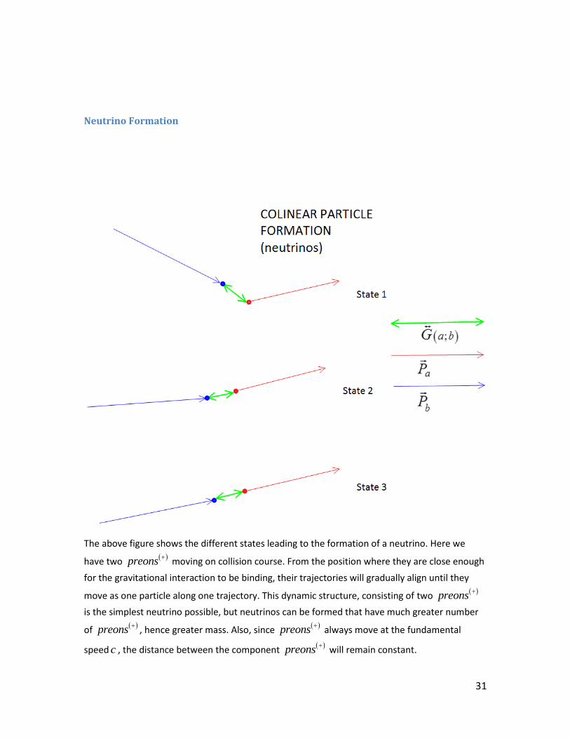
Neutrino Formation
The above figure shows the different states leading to the formation of a neutrino. Here we
have two
preons
moving on collision course. From the position where they are close enough
for the gravitational interaction to be binding, their trajectories will gradually align until they
move as one particle along one trajectory. This dynamic structure, consisting of two
preons
is the simplest neutrino possible, but neutrinos can be formed that have much greater number
of
preons
, hence greater mass. Also, since
preons
always move at the fundamental
speed c , the distance between the component
preons
will remain constant.
32
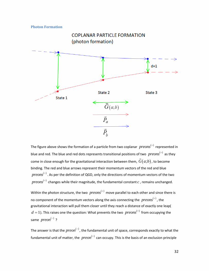
Photon Formation
The figure above shows the formation of a particle from two coplanar
preons
represented in
blue and red. The blue and red dots represents transitional positions of two
preons
as they
come in close enough for the gravitational interaction between them, ;G a b , to become
binding. The red and blue arrows represent their momentum vectors of the red and blue
preons
. As per the definition of QGD, only the directions of momentum vectors of the two
preons
changes while their magnitude, the fundamental constant c , remains unchanged.
Within the photon structure, the two
preons
move parallel to each other and since there is
no component of the momentum vectors along the axis connecting the
preons
, the
gravitational interaction will pull them closer until they reach a distance of exactly one leap(
1d ). This raises one the question: What prevents the two
preons
from occupying the
same
preon
?
The answer is that the
preon
, the fundamental unit of space, corresponds exactly to what the
fundamental unit of matter, the
preon
can occupy. This is the basis of an exclusion principle
33
by which a
preon
can only be occupied by a single
preon
. So a leap to a
preon
in
direction of the gravitational interaction is forbidden when the
preon
is already occupied by
another
preon
. Thus the gravitational interaction between will keep it two
preons
bounded and moving on parallel trajectories.
The exclusion principle also applies if the
preons
in the above figure arrive at a distance
2d but in this case, two outcomes are possible.
Neither
preon
leap to the middle
preon
and the distance between the blue and read
preons
will remain at 2d or
One of
preon
makes the leap to the middle
preon
while other is forbidden by the
exclusion principle. This will bring distance to 1d .
Though the outcome may be different, the photons having 1d between the
preons
of a
are indistinguishable from those where 2d .
Note that the photon given in this example is the simplest photon, one that is composed of only
one pair of
preons
. More massive photons will have any number of such bounded pairs.
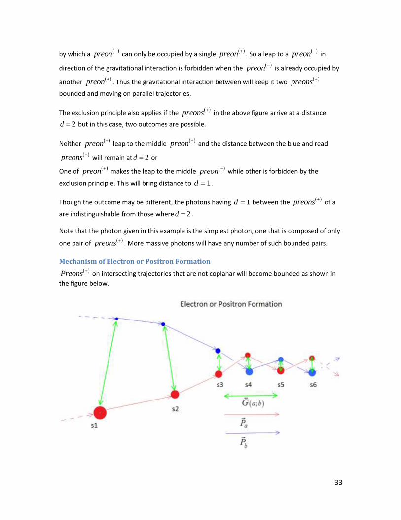
Mechanism of Electron or Positron Formation
Preons
on intersecting trajectories that are not coplanar will become bounded as shown in
the figure below.
34
In non-coplanar intersection, the momentum vectors of the
preons
will have non-zero
components along the axis of direction the gravitational interaction vector. This non-zero
component will keep the component
preons
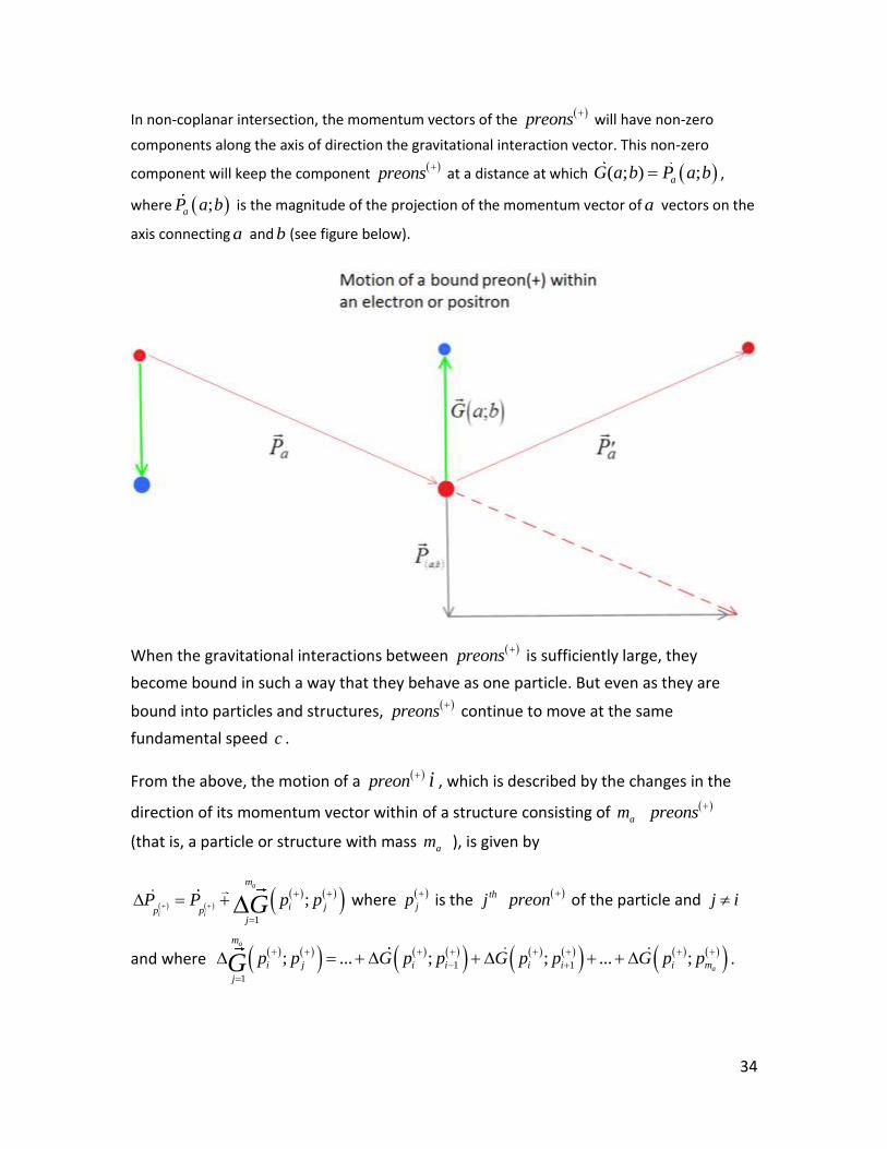
at a distance at which ( ; ) ;aG a b P a b ,
where ;aP a b is the magnitude of the projection of the momentum vector of a vectors on the
axis connecting a and b (see figure below).
When the gravitational interactions between preons
is sufficiently large, they
become bound in such a way that they behave as one particle. But even as they are
bound into particles and structures, preons
continue to move at the same
fundamental speed c .
From the above, the motion of a preon
i , which is described by the changes in the
direction of its momentum vector within of a structure consisting of am preons
(that is, a particle or structure with mass am ), is given by
1
;a
i i
m
i jp pj
P P p pG
where jp
is the thj preon
of the particle and j i
and where 1 1
1
; ... ; ; ... ;a
a
m
i j i i i i i m
j
p p G p p G p p G p pG
.
35
At the fundamental scale, the effect of n-gravity becomes negligible so that
1
; 1am
i j a
j
p p m kG
. Hence the force binding preons
is perhaps hundreds of
orders of magnitude larger than gravitational interaction at the Newtonian scale.
Here, what keeps the
preons
from one another is the component of ;aP a b along the axis
that connects a and b , which opposes the gravitational interaction. So, since 1a bm m , for
two preons at 1d we have 2
; 12
a b
d dG a b m m k k
, it implies that 1c k .
The reader will recall that g
kg
where g
is the magnitude of the p-gravity interaction acting
between two
preons
and g is the magnitude of n-gravity interaction between two
preons
.
Also, as we will see in the chapter titled Forces, Effects and Motion, the momentum of an
electron is the magnitude of the sum of the momentum vectors of its component
preons
or
as we will see in a later section, 1
em
iei
P c
wheree
P is the momentum vector of the
electron, e
m is the mass of the electron and ic is the momentum vector of its thi
preon
.
Since its energy is1
em
iei
E c
, it follows that the momentum of an electron or positron is
always smaller than its energy, unless it is accelerated to c ; in which case, since the
preons
components will be moving parallel to each other we will have 1 1
e em m
i i
i i
c c
and
e eE P . Thus, an electron or position accelerated to c will have the same structure as the
photon and since it is the helical motion of their component
preons
which determines their
physical properties, it follows that at speed c , an electron or positron become a photon.
36
Matter and Anti-matter (or the quantum-geometrical dynamics of electrons and
positrons and the electromagnetic effect.
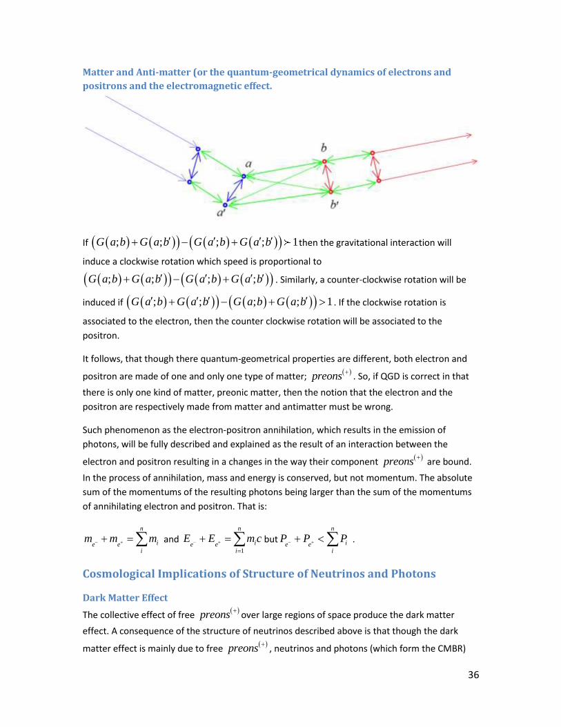
If ; ; ; ; 1G a b G a b G a b G a b then the gravitational interaction will
induce a clockwise rotation which speed is proportional to
; ; ; ;G a b G a b G a b G a b . Similarly, a counter-clockwise rotation will be
induced if ; ; ; ; 1G a b G a b G a b G a b . If the clockwise rotation is
associated to the electron, then the counter clockwise rotation will be associated to the
positron.
It follows, that though there quantum-geometrical properties are different, both electron and
positron are made of one and only one type of matter;
preons
. So, if QGD is correct in that
there is only one kind of matter, preonic matter, then the notion that the electron and the
positron are respectively made from matter and antimatter must be wrong.
Such phenomenon as the electron-positron annihilation, which results in the emission of
photons, will be fully described and explained as the result of an interaction between the
electron and positron resulting in a changes in the way their component
preons
are bound.
In the process of annihilation, mass and energy is conserved, but not momentum. The absolute
sum of the momentums of the resulting photons being larger than the sum of the momentums
of annihilating electron and positron. That is:
n
ie ei
m m m and 1
n
ie ei
E E m c
butn
ie ei
P P P .
Cosmological Implications of Structure of Neutrinos and Photons
Dark Matter Effect
The collective effect of free
preons
over large regions of space produce the dark matter
effect. A consequence of the structure of neutrinos described above is that though the dark
matter effect is mainly due to free
preons
, neutrinos and photons (which form the CMBR)

37
also contribute to the dark matter effect. The gravitational interaction between the “dark
matter” of a region R and an object a is given by
2
;2
D CNB CMBR ap
d dG R a m m m m k
where
pm , CNBm and CMBRm are
respectively the mass of free
preons
, neutrinos and the CMBR in R and d the distance
between the centers of gravity of the region R and the object a . At the current phase of the
evolution of the Universe, the mass of free
preons
appear to account for most of the dark
matter effect, but that will change as more massive structures are formed.
Note that established physics theories consider photons to be massless and neutrinos to have a
negligible mass so that they are not taken into consideration when calculating gravitational
interactions at the cosmic scale. Also, since their model of matter does not explain the dark
matter effect, established theories assign it to some exotic matter. QGD’s explanation does not
require exotic matter.
The dark matter effect is further discussed here.
The Preonic Field
Free
preons
exist throughout quantum-geometrical space for the preonic field, and though
they interact weakly, over large enough regions and close enough distance, they collectively
interact significantly with matter.
One important interaction is that between so-called charged particles and the preonic field. The
free
preons
in proximity of a charged particle interact with it so as to change their directions
and doing so, somewhat polarize the preonic field. The
preons
in close proximity will be
absorbed and reemitted by the charge particle. When absorbed, the
preons
will impart their
moment to the charged particle creating the effect who know as the electromagnetic effect. We
will discuss the electromagnetic effect in the chapter titled Forces, Effects and Motion.

38
A Brief Discussion on the Concept of Time The single most misleading concept in physics is that of time.
Although time is a concept that has proven useful to study and predict the behaviours of
physical systems (not to mention how, on the human level, it has become an essential
concept to organize, synchronize and regulate our activities and interactions) it remains
just that; a concept.
Time is a relational concept which is made to allow us to compare events with periodic
systems; in other words, clocks. But time has no more effect on reality than the clocks
that are used to measure it. In fact, when you think of it, clocks don’t really measure
time. Clocks count the number of recurrence of a particular state. For instance, the
number of times the pendulum of a clock will go back to a given initial position. So
clocks do not measure time, they count recurrent states or events.
Time is a relational concept essential to modeling reality but like any mathematical
model, it is a second order construct1. That is, it is not a property or aspect of physical
reality. Time is a concept and, for the purpose of representation of change relative to
periodic systems, one that can and has been viewed as mathematical dimension. But it
is essential in physics to distinguish mathematical dimensions from physical dimensions.
Unlike space, which physical properties affect reality, time has no effect, no incidence
on it. In fact, saying that time has an effect on reality is akin to saying that adding a zero
to the number of sheep in a field changes their actual count in reality. Changing an
aspect of reality affects its representation, but changing a representation does not
inversely affect the aspect of reality it represents.
Therefore, theories that unify space, which is physical, to time, which is not, are
confusing a purely conceptual construct with a fundamental aspect of physical reality.
And, if time doesn’t not exist, by extension, neither does space-time. This, as you may
have guessed, has profound implications on the way we understand reality. For
instance, if space-time does not exist, then all theories which assume its existence can,
at best, be approximation of reality.
In order to be consistent that it be rigorously developed from its axiom set, quantum-
geometry dynamics must strictly avoid using any concept or definition that doesn’t
correspond to an aspect of physical reality. This excludes the concept of time from
1 A first order representation is one that has a direct correspondence to physical reality. The
measurement of displacement of an object “a” is a first order representation. The ratio of the displacement of an object over the displacement of another is a second order representation.
39
quantum-geometry dynamics completely. But how can we describe reality without
time? Nearly all descriptions of dynamics systems require the use of time. How, for
instance, can we define speed, momentum, the laws of motion, all of which being time
dependant, without the concept of time?
Describing reality without using some concept of time must appear impossible, but I can
assure the reader that not only is it possible, it is not all that difficult once you apply the
principles of QGD.
Clocks The fact is: clocks do not measure time. They never have. Clocks are counting devices. What
they count is the recurrences of a particular physical state of its inner mechanism, which itself is
causally related to all preceding and successive states. This means that there are identifiable
physical mechanisms that causally link a clock's different states. Unlike spatial measuring
devices, which relate to the physical aspect of reality we call space, there is no relation
whatsoever between clocks and a physical aspects of reality. Clock count the ticks of the clock,
nothing else.
Time Distance Equivalence A simpler way and physical way to measure the duration of an event is to mark its start and end
and measure the distance a photon will travel between these two marks. This provides
measurement of duration that is based on actual physical quantities.
On The Concept of Simultaneity
It seems obvious that when we talk about simultaneity, we are talking about
simultaneous events.
In the classic sense, simultaneity describes events which an observer perceives has
happening at the same time. While relativistic simultaneity is observer dependant, QGD
simultaneity is absolute.
But before we can define simultaneity, we must define what an event is.
Definition of an event:
Quantum-geometry dynamics defines an event as the interaction of two particles
which have come close enough to locally interact in a way that changes their structure
and direction.
An example of an event is the formation of an electron from two photons. Such an
event is characterized by two photons (the particles), the regions where the interaction
takes place (the preons
which along the photons’ paths which intersect at a QGD
distance of), the formation of an electron (change in structure) and change in direction.
40
To describe interactions of complex structures that change their structures and
directions, we will use system of events.
For example, when an electron and a positron converge in such a way they annihilate
one another resulting in the emission of photons, the system of events is comprised of
two events, each one resulting in the production of photons.
Also, events, as everything else in the Universe, obey a law of conservation.
Theorem of Instantaneity of Gravitational Interactions
The gravitational interaction between any two preons
or between any two
preons
-
charged preons
anywhere in the Universe is the same regardless of the quantum-
geometric distance that separates them.
What this implies is that, contrary to general relativity which holds that gravity
propagates at the speed of light; gravitational interactions are, for lack of a better term,
instantaneous.
As we recall from, preons
and
preons
are fundamental so require the pre-
existence of no other physical entities. The same is true of their associated force.
Now, according to QGD, the force acting between two preons
is one of negative
gravity which is responsible for the dimensionalization of quantum-geometric space.
The force acting between two preons
is not, as current models hold, a function of
metric distance. Metric distance is a purely mathematical concept. Since metric distance
has no physical reality, it has no influence on reality.
This means that any change in the structure of an object (which as we have seen are due
to systems of events) instantly changes the gravitational interactions between this
object and all other objects in the Universe.
Definition of Simultaneity
Two distinct events affecting two distinct objects are simultaneous if the objects interact
gravitationally as the events occur.
In other words, the events coexist. This definition of simultaneity makes use of the
nature of gravitational interactions, which, as we recall are instantaneous. This
definition of simultaneity, which requires that gravity be instantaneous, is independent
of the distance between the objects and is consequently observer independent.
The inclusion of an observer in the definition we get:
41
Three distinct events, affecting three distinct objects, one of which being an observer, if
the objects interact gravitationally as the events occur.
Precedence
Considering two events affecting one object, one event succeeds the other if the state
the object is in when experiencing the event is causally dependant on the state the
object is in when experiencing the other.
Also, considering two eventsaE and
bE respectively affecting two distinct objects a and
b , thenaE precedes
bE if the state
aS of a is simultaneous with
bE and
aS is causality
dependant onaE ; that is,
aS results from
aE .
From the above theorems we can derive the following:
Second Theorem of Simultaneity
Two events are simultaneous if the variations they cause in the gravitational interactions
are additive.
What this means is that, if events are simultaneous, the individual changes in
gravitational interactions are felt as one single change which is equal to the sum of the
changes brought about by the individual events.
The theorem of instantaneity of gravitational interactions does imply that faster than
the light travel is possible – unlike interactions, matter is subjected to the physical
limitations of propagation imposed by the quantum-geometric structure of space – but
information, in the form of gravitational fluctuations, may theoretically be transmitted
instantly between any two points in the Universe.
Principle of Strict Causality The principle of strict causality implies that all states and events are causality dependant on
preceding states or events.
If, as QGD implies, time does not exist, then time playing no role on events, no events can be
probabilistic, hence none can be spontaneous. That means that all events, even those which
appear spontaneous must be caused discrete interactions between at least two distinct objects
or two components of an object.

42
Forces, Effects and Motion A premise of quantum-geometry dynamics is that there exist only two fundamental
forces; n-gravity and p-gravity which are respectively carried by preons
and
preons
.
Preons
, the reader will recall, are particles which dimensionalize space and preons
are the fundamental particles of matter.
As a consequence all interactions must be quantum-geometrical effects of n-gravity and
p-gravity. This in turn implies that all interactions are emergent and, as we will see, may
be described from a single general equation which gravity, electromagnetism, the weak
interaction, nuclear forces, the dark matter effect, the dark energy effect and all and any
forces which may be observed in the future are all particular solutions of.
We will also show that wide differences in the orders of magnitude of the above forces
can be fully explained from the dynamics of the quantum-geometric structures of the
interacting particles or bodies.
The Gravity Effect
Currently, gravity is considered a fundamental force which acts between massive
structures and which magnitude is a function of mass and distance. It is considerd the
weakest of the four forces identified by current physics theory.
QGD proposes that gravity be not a fundamental force, but the resultant of the
compound effects of n-gravity and p-gravity. If all massive structures are subjected to
opposing forces of n-gravity and p-gravity, then gravity is the net result of these
influences.
We will show that the gravity effect only appears to be weak because n-gravity and p-
gravity are in near equilibrium at the molecular and larger scale of reality.
Imagine a giant balance scale with pivot point having negligible friction. Placed on each
of the two pans are two identical structures weighing exactly one million kilograms
each. Now, if as we mentioned, friction is negligible, very little force is necessary to tip
the scales one way or the other. In fact, a feather would suffice. But if we had only one
or the other million kilogram object on the balance scale at once, it would take
enormous force to tip the scales.
Though the analogy above is imperfect, it is correct in the way that a similar reasoning
applies to the opposing influence of n-gravity and p-gravity. P-gravity and n-gravity are
the most powerful forces in the Universe (with p-gravity being k times greater than n-

43
gravity) but at non fundamental scales, they are in near equilibrium and very little force
is needed to break balance between p-gravity and n-gravity.
But at the fundamental level, where matter is a lot denser, p-gravity is not balanced by
n-gravity. As a result, the gravity effect is orders of magnitude greater than that
between objects at the non-fundamental scale.
This is the reason why it takes proportionally little force to escape the gravity of the
Earth compared to the energy needed pull an atomic nucleus apart.
Gravity effect between preons(+).
The fundamental interaction, which provides the basis for calculating gravity, is that
which exists between two preons
.
We already established that the force acting between any two preons
is the
fundamental unit of p-gravity, ,g but the gravitational interaction between them must
also take into account the interactions between the preons
between them.
For two preons
, a and b , moving in the same direction on parallel trajectories at a
distance equal to d , the gravitational interaction between them, gravity, is given by:
2
;2
d dG a b k
where the quantum-geometric distance d is equal to the number of preons
on the
line connecting the preons
and
2
2
d d is the count of all n-gravity interactions
between a and b .
The magnitude of the p-gravity interaction between the two preons
expressed in n-
gravity units is equal to g , which is equal to kg .
Also, participating in the interaction, are the preons
along the line connecting
preons
a and b which interact with the
preon
s and with each other. The
magnitude of the n-gravity interactions between two preons
is the number of such
interactions or 2
2
d d n-gravity interactions.
44
So the gravitational interaction between two preons
is the resultant of the n-gravity
and the p-gravity between them. To express this using single integer units, one has
simply to count the number of p-gravity interactions and the number of n-gravity
interactions, convert the p-gravity value in the equivalent n-gravity value using the
relation g kg , then add the results.
In our example, if 2 ( ) / 2k d d then the net gravitational interaction or gravity is null
and the preons
will have no effect on their respective trajectories.
If 2 ( ) / 2k d d then gravity is positive and the preons
’s trajectories will be
affected and they will move toward each other in accordance to the QGD law of motion
described later in this chapter.
Finally, if 2 ( ) / 2k d d , then the preons
will move away from one another at a rate
proportional to ( ; )G a b and in accordance to QGD’s law of motion.
Gravity effect between structures
Gravity between two structures is calculated in a similar way. If objects a and b
respectively have am and bm preons
then the gravity between them is given by
2
, ,
11
;2
b
a
mm
i j i j
a b
ij
d dG a b m m k
where i and j are indexed
preons
of a and b , which
equation describes gravity at all scales. But larger scales we find that
2 2, ,
11
2 2
b
a
mm
i j i j
a b
ij
d d d dm m
, where d is the distance between the centers of gravity of
a and b so that we may use 2
;2
a b
a b
m m d dG a b km m
.
This last equation can be written simply as 2
; ( )2
a b
d dG a b m m k
though it is
important when using this form to remember the combinatorial origin of the equation.
The gravitational effect equation 2
; ( )2
a b
d dG a b m m k
, which is derived from the
axioms of QGD bares some comparison to 1 2
2
GM MF
d , Newton’s Law of Universal

45
Gravitation. Both describe the magnitude of gravity between two bodies as being
proportional to the product of their masses. There are also some important differences.
The first is that Newtonian gravity is a fundamental force whence the QGD equation
implies that gravity is the resultant effect of the two fundamental forces; p-gravity
which is a fundamental attractive force carried by preons
and n-gravity, the
fundamental repulsive force carried by preons
.
The second is that the Newtonian gravity implies that space is continuous and that it is a
passive medium while, according to QGD, space is discrete (quantum-geometrical) and
is generated by the n-gravity field of preons
. Therefore
preons
dynamically
participate in the gravitational interactions between bodies.
The third difference is that gravity in the Newtonian equation is strictly positive. The
QGD equation also allows for gravity to have a null value when2
2
d dk
or a negative
value when2
2
d dk
. Negative values account along with polarized
preons
, similar
to those responsible for electromagnetic effect, participate in the observed dark energy
effect.
It follows that Newton’s Law of Universal Gravitation must be an approximation of the
QGD gravitational effect equation for distances such that2
2
d dk
, that is , where p-
gravity is greater but in near equilibrium with n-gravity.
Thus, the gravity effect at the Newtonian scale is approximately proportional to inverse
to the square of the distance which is an approximation of the QGD equation that shows
gravity to be proportional to the difference between the p-gravity interaction given by
a bkm m and the n-gravity interactions given by 2 / 2a bm m d d .
General Application of the QGD Gravity Equation
The QGD gravity equation can be used to calculate the gravitational interactions
between any physical objects. It matters not that the objects be elementary, molecular,
planetary, cosmic or any combination of the above. The QGD equation will be used
below to derive the laws of motion.
It is essential that we remember to use the form of the QGD gravitational equation that
is appropriate for the scale at which we apply it. That is the form
46
2
, ,
11
;2
b
a
mm
i j i j
a b
ij
d dG a b m m k
must always be used for interactions at the microscopic
scales and particularly when describing the motions of particles and applying it to
describe optics. At larger scales, where 2 2, ,
11
2 2
b
a
mm
i j i j
a b
ij
d d d dm m
, the form
2
; ( )2
a b
d dG a b m m k
is a close approximation and should be used.
As discussed earlier, quantum-geometry dynamics proposes that there be only two
fundamental particles: The preon
, which dimensionalizes space, and the
preon
, the
fundamental particle of matter. What distinguishes quantum-geometry dynamics from
dominant theories of fundamental physics, collectively known as the standard model, is
that all properties of elementary particles are intrinsic. Essentially, this means that no
additional particles and their properties are necessary to explain interactions not only at
the fundamental scale but at all scales.
According to QGD, every particle or material structure is made of preons
. That
includes, without exception, all particles we currently consider to be elementary.
Electrons, positrons, neutrinos and even photons are thus composed of preons
.
Preons
possess two intrinsic properties. The first is that they are strictly kinetic.
Preons are always in motion. Their speed is fundamental and equal to c . The speed
of preons
is constant whether they are free or bound within a composite particle or
structure. The constancy of the speed of preons
is a direct consequence of the
quantum-geometrical structure of space. preons
move by leaping from
preon
to
preon
. The preonic leap is fundamental unit of distance. Since there is no smaller
distance than the preonic leap, there is no faster motion than that of a preon
.
The second intrinsic property of preons
is that they interact with each other through
p-gravity, which is an attractive force acting between them. The p-gravity interaction
between two preons
is the fundamental unit of p-gravity or g .
47
Mass
Quantum-geometry dynamics considers mass to be an intrinsic property of matter. It
follows that since preons
are the fundamental particle of matter, their mass must be
the fundamental unit of mass. It follows that the mass of an object should be
understood as being equal to the number of preons
it contains. So when we write
that am is the mass of a particle a we mean that it contains m number of preons
.
Side note about black holes
It follows from the quantum-geometric structure of space that the maximum density of a black hole is limited (as it is for any other structure). The maximum theoretical density of any
structure is equal to 1
preon
/2
preons
. So assuming a black hole having a radius equal
to r which has achieved maximum density, then its maximum mass would be equal to 32
3
r
preons
. As for all measure of distance in QGD, the value of r is given in preons(=). The
maximum mass given here is an upper boundary based on the maximum theoretical density. The actual mass of a black hole should be lower by orders of magnitude. See the section Black Holes and Black Hole Physics for a detailed discussion about black holes.
Energy
Energy is an intrinsic property of preon
. The fundamental unit of energy corresponds
to the kinetic energy of the preon
, its momentum, which is equal to c .
From the above, we can define the total energy of an object as1
am
a i a
i
E c m c
where
am is the mass of a in preons
and ic are the momentum vectors of each of it
component preons
. For a single
preon
we have 1p
m so ipE c c .
QGD defines the speed of a body as the ratio of its momentum to its mass or
1
1 am
a i
ia
v cm
.
It is important here to remember that though the momentum of a preon
is
numerically equivalent to its speed, momentum and speed are two distinct properties.
They are numerically equivalent in special cases, but physically distinct.
48
The above equation applies to composite particles or structures. So if a is a particle or
structure with mass am , then its energy must correspond to the added energies of the
preons
that compose it. In mathematical terms the relationship between energy and
mass is expressed by the equation a aE m c ; the number of preons
multiplied by the
kinetic energy of each preon
.
Thus quantum-geometry dynamics provides a simple and elegant explanation of the
relationship between the mass of a body and its energy. It is important to note though
QGD's equation appears to be similar to Einstein’s mass-energy equivalence equation, it
differs in important ways.
First, a aE m c is not an equivalence relation between mass and energy. Mass
corresponds to the number of preons
of a body and energy corresponds to the
number of preons
multiplied by the fundamental momentum of a
preon
or c . So
the QGD equation expresses a proportionality relation between mass and energy, not
an equivalence relation. So according to the QGD model, mass can never be converted
to energy, nor energy be converted to mass. Mass and energy are two distinct
properties of matter.
At first glance this may appear to contradict observations. For instance, nuclear
reactions result in a certain amount of mass being transformed into energy. What the
QGD model suggests is that during a nuclear reaction, mass is not transformed into
energy, but rather, bound particles become free from the structures they were bound to
and carry with them their momentum. There is no conversion of mass into energy, but
only the release of particles having momentum. We will see in the next section how
kinetic energy is the only kind of energy that exists.
Momentum
That mass and energy are intrinsic properties of preons
implies that unless a
composite particle or massive structure loses or acquires preons
, its mass and energy
remains constant regardless of its speed. This is in disagreement with dominant physics
theories which define the energy of an object has the sum of its intrinsic energy, also
known as its energy at rest, and its kinetic energy or momentum; a relation that is
expressed by the equation 2E mc mv where 2mc is the energy of the body at rest, c
the speed of light, and mv ,the product of the its mass by its speed v ,its kinetic energy
or momentum.

49
The accepted definition of the energy of a body is logically correct. The reasoning
behind it is simple. In order to accelerate an object, one needs to impart energy to it.
Thus it makes perfect sense that the accelerated object carries this added energy, which
we call kinetic energy, with it. So the assumption that the total energy of body must be
equal to the energy it had prior to acceleration plus the kinetic energy that is imparted
to it is perfectly logical. However, we will show here that using the axioms of QGD we
arrive at different descriptions and explanations which, though in disagreement with
dominant physics theories, are consistent with observations.
According to QGD, there is only one kind of energy known as kinetic energy or
momentum.
As explained earlier, the momentum of a preon
is constant, hence its speed is
constant and equal to c . It follows that the total energy of a particle or massive
structure must be equal to the sum energy of its constituents. This is described by the
equation a aE m c .
From this point we will use vectors to represent momentum and direction. We will, for
example, associate the vector c to the momentum of a preon
so that c c . The
energy of a preon
is thus the magnitude of its momentum vector. This distinction
allows us to define aE and aP , respectively the energy and momentum of a particle a in
the following way:
1
am
a i a
i
E c m c
and 1
am
a i
i
P c
.
To illustrate this, let's consider the simple
particle made of two bound preons
as
shown in the following figure 1.
Here the particle, which we’ll denote a , is
composed of two preons
, 1p
and 2p ,
bound by gravitational interaction (the
resulting effect of p-gravity and n-gravity).
The purple arrows represent their
trajectories in quantum-geometrical space.
The yellow vectors represent their
momentum at a certain point before taking

50
into account the bounding force 1 2;G p p . This magnitude of this vector is equal to
c .
In this example, the interaction between the preons
are strong enough to deviate
them from what would be their free trajectories, which would coincide with their
momentum vector.
If the composite particle in our example is not subjected to any other force, then
1
2am
a i a
i
E c m c c
, and its momentum is1 2
1
0am
a i
i
P c c c
. The zero value
indicates that particle is at rest relative to quantum-geometrical space.
However, if a interacts with a massive structure b
(see figure 2), then the trajectories of the preons
of
1p and
2p will change and affect the momentum of
a . We still have 2aE c but that 1 2 2a aP c c v
whereav is the speed of the particle.
This example shows how the energy of a particle does
not change as a function of its speed. The momentum
of a particle changes but momentum is already taken
into account in the equation a aE m c . The same
applies to material structures at all scales.
We should address here the issue of the maximum
possible speed of massive structure. From what we have seen so far, the speed of any
structure is1
ai
a
a
i
mPc v
m
. Since1 1
max i i
a a
i i
m m
c c
, the maximum speed of a
particle or structure is achieved when the momentum of a particle is equal to its energy
or a aP E . This is evidently the case for photons, but that shouldn’t be confused with
current idea that light is pure energy. The energy of a photon is still that of its
component preons
. The same applies to any structure when the trajectories of all its
component preons
are parallel and oriented in the same direction. In such special
case we have1
a i a
a
i
m
P c m c
so that a aa
a a
P m cv c
m m . Particles for which energy
51
and momentum are always equal include photons and neutrinos but theoretically any
structure regardless of its mass can achieve c if it is submitted to a strong enough force.
Slowing Down of Clocks
QGD considers time to be purely a relational concept. In other words, time is not an aspect of physical reality. But if time does not exist, how then, how does QGD explain the different experiments which results support time dilation; the phenomenon predicted by special relativity by which time for an object slows down as its speed increases. To explain the time dilation experiments we must remember that clocks do not measure time, they count the recurrences of a particular periodic system. The most generic definition possible of a clock is a system which periodically resumes an identifiable state and a counting mechanism that counts the recurrences of that state. Clocks are physical devices and thus, according to QGD, are made of molecules, themselves made of atom composed of particles and those particles; all of which are ultimately made of
bounded
preons
.
We know that the magnitude of the momentum vector of a
preon
is fundamental and
invariable. The momentum vector is denoted by c the momentum is c c . We have shown
that the momentum vector of a structure is given by 1
am
a i
i
P c
and its speed by 1
am
i
i
a
a
c
vm
. From these equations, it follows that the maximum possible speed of an object a corresponds
to the state at which all of its component
preons
move in the same direction. In such case we
have 1 1
a am m
i i a
i i
c c m c
and aa
a
m cv c
m . Note here that
1
am
i
i
c
corresponds to the
energy of a so the maximum speed of an object can also be defined at the state at which its momentum is equal to its energy.
From the above we see that the speed of an object must be between 0 and c while all its
component
preons
move at the fundamental speed of c .
Now whatever speed a clock may travel, the speed of its component
preons
is always equal
to c . And since a clock’s inner mechanisms which produces changes in states depend
fundamentally on the interactions and motion of its component
preons
, the rate at which
any mechanism causing a given periodic state must be limited by the lowest inner motion which
is transversal speed of its component
preons
.
Simple vector calculus shows that the transversal speed of bound
preons
is given by
2 2
ac v where av is the speed at which a clock a travels. It follows that the number of
recurrence of a state, denoted t for ticks of a clock, produced over a given reference distance
refd is proportional to the transversal speed of component
preons
, that is

52
2 2
a
ref
tc v
d . It is thus easy to see that as the speed at which a clock travels is increased,
the rate at which it produces ticks slows down and that becomes 0 as its speed approaches c . We have thus explained the observed slowing down of periodic systems without resorting to the concepts of time or time dilation. So though the predictions of special relativity in regards to the slowing down of clocks (or any physical system whether periodic or not, or biological in the case of the twin paradox) are in agreement with the predictions QGD. QGD explanation however is based in fundamental aspects of reality. Also, since according to QGD, mass, momentum, energy and speed are being intrinsic properties of matter, their values are independent of any frame of reference thus avoiding the paradoxes, contradictions and complications associated with frames of reference. However, though both QGD and special relativity predict the effect of speed on clocks, there are important differences in their explanation of the phenomenon and the quantitative changes in rate. While for special relativity the effect is caused by a slowing down of time, QGD explains that it is a slowing down of the mechanisms clocks themselves.
If t and t are the number of ticks counted by two identical clocks counted travelling
respectively at speeds av and av over the same distance refd then QGD predicts that
2 '2
2 2
a
a
c vt t
c v
.
This prediction distinguishes QGD from special relativity’s prediction that2 2
1t t
c v
.
However, it is important to note that the two predictions of the QGD and the special relativity equations cannot be directly compared. The speed in the relativist equation is the relative speed of the clocks while the QGD equation makes uses the distinct and intrinsic speed of the clocks. Slowing Down of Clocks due to Gravity
Since a
a
a
Pv
m then
2 2 2 a
a
ref a
Ptc v c
d m . We have also shown that gravity affects
the orientation of the component
preons
of structure so that ;aP G a b . So given
that we know that the rate of a clock a at a given distance 1d from a massive body b , that is
21 a
ref a
Ptc
d m . Then moving the clock to either closer or further from b to 2d , we will
find that
22;a
ref a
P G a btc
d m
where 1 2; ; | ; |G a b G a b d G a b d .
As we can see, the greater the gravitational interaction between a clock and a body, the slower will be its rate. This prediction is also in agreement with general relativity’s prediction of the slowing down of clocks by gravity.

53
Conclusion and Implications We have shown that the slowing down of clocks resulting from increases in speed or the effect gravity is explained not as a slowing down of time, but as a slowing down of their intrinsic mechanisms. The effects of the time dilation predicted by special relativity and general relativity are both
described by
2;a
ref a
P G a btc
d m
since it takes into account both the effect of the
speed and gravity on a clock. Thus, if QGD is correct, the predictions of SR and GR are approximations of particular solutions of the QGD equation. We will see later how QGD can predict the behaviour of binary pulsar systems and explain and predict the decay of atmospheric muons, both phenomenon supporting special relativity and general relativity. The decay of muons is particularly significant as provides indirect evidence in support QGD’s prediction that they (and all other elementary particles) have structure and are composed of
preons
.
Calculating Direction of a Bound Preon(+) and Structures
When a preon(+), denoted p
, is subjected to an interaction with an object a , expressed by
force vector ;G p a
, its direction changes while its speed, hence its energy remains
constant and equal to c . The momentum of a
preon
is conserved under change in
direction.
If c is the momentum vector of a
preon
and 'c is its momentum vector resulting from a
change in direction cause by attractive force, then 'c c c . The momentum is conserved
in accordance to the equation 'c
c c Gc G
for a single
preon
influenced by a single
forceG (note: this is a solution of the directional sum introduced earlier whereaP c ).
When a
preon
is subjected to n forces we have 1
1
'n
ini
i
i
cc c G
c G
. Also, because
the momentum vector of a particle or massive structure is the resultant of the sum of the

54
momentum vectors of all its components, that is1
a a i a a
a
i
m
P m c m v
, and we can threat the
particle as a whole when it is subjected to a force. Then using the momentum vector aP for the
particle a can have ' ;a aP P G a b where ;G a b is the gravitational interaction between
a andb and ;
;a
G a bG a b
m
. Similarly ;
;b
G a bG b a
m
.
In conclusion, change in speed and the corresponding change in momentum of a composite
particle or massive structure is caused by discrete changes in the trajectories of their
component
preons
. The kinetic energy of a composite particle or structure is thus a
directional component of the total energy along the axis of motion. As such, the kinetic energy
of body is already included in the intrinsic energy of an object, itself the sum of the kinetic
energy of its
preons
. At the most fundamental scale, the preonic scale, since
preons
are
kinetic, there is no such thing as rest mass. But there can be, as we saw earlier, non-
fundamental structures in which the momentum vectors cancel out resulting in a null net
momentum.
As the reader can see, the equation E mc naturally emergences from the axioms of quantum-
geometry dynamics.
Understanding how energy is conserved under acceleration is a simple shift with important
impact in physics. In cosmology, for example, a universe which undergoes an accelerated
expansion does not violate the law of conversion of energy the way relativistic acceleration
does. The energy of the galaxies undergoing acceleration does not change (except from the
variations of their masses). This also implies that the mass and energy of the Universe is
conserved.
Note: We will see in the coming article about gravity how the effect attributed to dark energy
can be attributed to negative a negative solution of QGD’s gravitational interaction equation
force (where n-gravity interactions exceed p-gravity interactions). We will also show why dark
energy cannot be detected by instruments.
Why No Higgs Mechanism?
How can QGD prediction that there is no Higgs boson or mechanism when its discovery
has been announced and hugely publicized?
First, it is important to know that the particle that was discovered was not the Higgs
boson but a Higgs-like particle. What exactly does that mean? Well, it means that a
particle was discovered which displays some properties that are in agreement with what
the standard model of physics predicts the Higgs boson should have. What is less

55
understood is that the discovered particle also possesses properties that are in conflict
with the predictions. But what we really mean by “no Higgs” is that whatever particle
has been or will be found, it does not convey mass through though the Higgs
mechanism or in any other way. Why?
Because QGD considers mass to be a fundamental property of matter, that is, it is an
intrinsic property of preons
.. Thus the mass of an object, expressed in fundamental
units, is simply the number preons
it contains (and energy, the number of
preons
.
times the fundamental unit of kinetic energy or momentum). So since mass is a property
of the preons
and all matter are made from
preons
then particles of matter do not
require the existence of the Higgs boson or anything similar to the Higgs mechanism to
convey mass. In fact, unlike gauge theories where many physical properties are
extrinsic, fundamental properties displayed by each of the two fundamental particles
are intrinsic to them.
That said, as mentioned earlier, the validity of a theory cannot be established from
within the framework of another when they are based on mutually exclusive axiom sets.
So, QGD can no more invalidate the Standard Model than the Standard Model can
invalidate QGD. Nature is the only arbitrator when it comes to the truth of a theory.
Calculating Direction of a Bound Preon(+) and Structures
When a
preon
, denoted p
, is subjected to an interaction with an object a , expressed by
force vector ;G p a
, its direction changes while its speed, hence its energy remains
constant and equal to c . The momentum of a
preon
is conserved under change in
direction.
If c is the momentum vector of a
preon
and 'c is its momentum vector resulting from a
change in direction cause by attractive force, then 'c c c . The momentum is conserved
in accordance to the equation 'c
c c Gc G
for a single
preon
influenced by a single
forceG .
When a
preon
is subjected to n forces we have 1
1
'n
ini
i
i
cc c G
c G
. Also, because
the momentum vector of a particle or massive structure is the resultant of the sum of the
56
momentum vectors of all its components, that is1
a a i a a
a
i
m
P m c m v
, and we can threat the
particle as a whole when it is subjected to a force. Then using the momentum vector aP for the
particle a can have ' ;a aP P G a b where ;G a b is the gravitational interaction between
a andb and ;
;a
G a bG a b
m
.
In conclusion, change in momentum and the corresponding change in speed of a composite
particle or massive structure is caused by discrete changes in the trajectories of their
component
preons
.. The kinetic energy of a composite particle or structure is thus a
directional component of the total energy along the axis of motion. As such, the kinetic energy
of body is already included in the intrinsic energy of an object, itself the sum of the kinetic
energy of its
preons
.. At the most fundamental scale, the preonic scale, since
preons
.
are kinetic, there is no such thing as rest mass. But there can be, as we saw earlier, non-
fundamental structures in which the momentum vector cancel out resulting in a null
momentum.
As the reader can see, the equation E mc naturally emergences from the first principles of
quantum-geometry dynamics.
Understanding how energy is conserved under acceleration is a simple shift with important
impact in physics. In cosmology, for example, a universe which undergoes an accelerated
expansion does not violate the law of conversion of energy. The energy of the galaxies
undergoing acceleration does not change (except from the variations of their masses). This also
implies that the mass and energy of the Universe are conserved.
Heat, Temperature and Entropy
Using the concepts we have introduced so far, we will now derive quantum-geometrical
explanation of the properties of heat, temperature and entropy.
Given a system S having n unbound particles, the heat of the system is equal to1
n
i
i
P
,
where iP is the momentum of the nti particle and its temperature is 1
n
i
i
S
P
Vol
.where SVol is
the volume of the system measured in preons
, the fundamental and discrete particle
which forms and dimensionalizes quantum-geometrical space. The total energy of the
57
system being equal to1
n
i
i
m c
, it follows that if we define entropy in the classical sense,
then the entropy of S is1 1
n n
i i
i i
m c P
.
Application to Exothermic Reactions within a System
The QGD definitions can be used to describe the changes in heat and temperature
resulting from chemical or nuclear reactions. The particles involved are different, as are
the reaction mechanisms, and the reactions occur at different scales, but both result in
changes in the structure and number of bound particles.
Consider 1 2S S where 1S is a dynamic system containing 1n unbound particles (or
structures) some of which reacting with each other, and 2S the resulting system
containing 2n unbound particles, if 2 1n n then1 2
1 1
'n n
i i
i i
P P
and the change in heat of
the system 2 1
1 1
'n n
i i
i i
PH P
is positive.
For example, let say the system contains only a particle e and a particle e which
annihilate to give n photons ( ), then 1
i
n
ee e ei
m c v mH v m
. Here, the
difference in heat depends on the speed of interacting electrons and is at the lowest
when electrons achieve the speed of light; in which case 0H .Note that from the
QGD model, when electrons achieve c , internal motion stops, so that component
preons
move in parallel trajectories.
Also, QGD predicts that electrons accelerated to c become indistinguishable from
photons and become electrically neutral. The electrical charge of a particle is caused
by internal motion of its component preon
which interact with the preonic field
(the free preons
populating quantum-geometrical space). Since all internal
motion stop at speed c , the electron moving at that speed must lose their electric
charge.
Also worth nothing is that 1
i
n
eei
m m m
which implies that1 2S SE E ,that is;
mass and energy are conserved. This holds for all closed systems. So though it is
believed that a nuclear reaction results in the conversion of mass into energy,
according to QGD, it results in the freeing of bound particles which carry with them
58
momentum, hence increase the heat of the system. Aside from the reaction
mechanism, the only difference between exothermic chemical and nuclear reactions
is in the type of particles that become free. For chemical reactions these particles are
molecules, atoms and photons and for nuclear reactions, nuclei and other subatomic
particles.
Application to Cosmology
In the initial state of the Universe, QGD theorizes that all preons
were free. That
means that the energy of the Universe was equal to its heat. So if that its entropy was
equal to zero. That is:1
0n
U i
i
m c P
, where Um is the masse of the Universe in
preons
and since all
preons
are free Um n . It follows that the temperature of
Universe in its initial state was 0
U U
U
m cT
Vol .
Though the Universe as evolved, its total energy remains Um c , but as particles and
structures are formed its heat decreases resulting in an increase in entropy according. In
formal terms we have 1
0n
U i
i
m c P
).
For those interested in reading further, the chapter on cosmology in Introduction to
Quantum-Geometry Dynamics explains that the temperature of the Universe in its initial
state and to the only two constants of QGD; c the kinetic energy of the preon
and k
the proportionality constant between the n-gravity and p-gravity, are related by the
equation 0
cT
k .
The coming article will discuss how gravity emerges from the interactions between
preons.
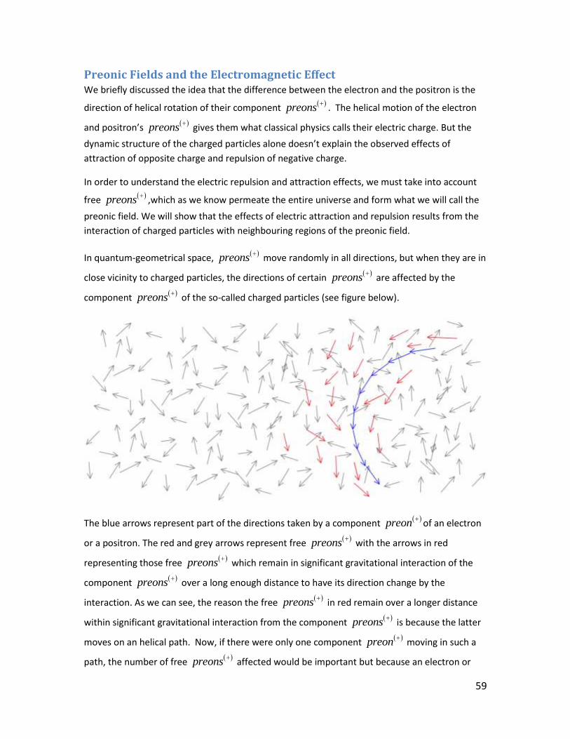
59
Preonic Fields and the Electromagnetic Effect We briefly discussed the idea that the difference between the electron and the positron is the
direction of helical rotation of their component
preons
. The helical motion of the electron
and positron’s
preons
gives them what classical physics calls their electric charge. But the
dynamic structure of the charged particles alone doesn’t explain the observed effects of
attraction of opposite charge and repulsion of negative charge.
In order to understand the electric repulsion and attraction effects, we must take into account
free
preons
,which as we know permeate the entire universe and form what we will call the
preonic field. We will show that the effects of electric attraction and repulsion results from the
interaction of charged particles with neighbouring regions of the preonic field.
In quantum-geometrical space,
preons
move randomly in all directions, but when they are in
close vicinity to charged particles, the directions of certain
preons
are affected by the
component
preons
of the so-called charged particles (see figure below).
The blue arrows represent part of the directions taken by a component
preon
of an electron
or a positron. The red and grey arrows represent free
preons
with the arrows in red
representing those free
preons
which remain in significant gravitational interaction of the
component
preons
over a long enough distance to have its direction change by the
interaction. As we can see, the reason the free
preons
in red remain over a longer distance
within significant gravitational interaction from the component
preons
is because the latter
moves on an helical path. Now, if there were only one component
preon
moving in such a
path, the number of free
preons
affected would be important but because an electron or
60
positron are made of a large number of bound
preons
the effect is greatly amplified. Not
only the gravitational interactions between the electron and the neighboring preonic region
much greater, but there is always there
preons
in red are always within significant
gravitational interaction with several bound
preons
.
Objects at larger scales are made of a great number of atoms, each made of bound
preons
.
When orientation of the electrons of the object is random, all free
preons
are affected and
randomness of their directions is not affected. But when the electrons in the object are
arranged in such a way that the directions of the electrons are aligned, the only the
preons
that are moving in the same general direction as the bound
preons
of our structure will be
affected by the gravitational interaction so as to change their direction. The larger the number
of aligned electrons in a structure, the greater will be the number of
preons
of the preonic
region neighbouring affected by the structure. This explains why some materials are magnetic
while others are not.
I’ve mentioned that for free
preons
to be affected, they must remain within significant
gravitational interaction over a long enough distance. We understand from the above what we
mean by “over a long enough distance” but what does “within significant gravitational
interaction” mean exactly?
A object a is within significant gravitational interaction of an object b when ; aG a b xm
where ;G a b is the gravitational interaction between a and b , am is the mass of a in
preons
and x N . The significant gravitational interaction is the minimum gravitational
interaction necessary to affect direction of an object (we will discuss this in detail in the chapter
on optics).
From the above definition we see that the more massive an electron is or the more of them
there are, the greater the gravitational interaction and the larger will be the preonic region
affected. The gravitational interaction between a
preon
and an electron is given by the
gravitational interaction equation. Substituting ( )p
and e for a and b , the gravitational
interaction equation becomes:
2
;2p e
d dG p e m m k
where d is understood as the average distance of
between the free
preons
and the component
preons
of the electron. Or, since 1p
m

61
we can write
2
;2e
d dG p e m k
. From this equation and we can see the
gravitational interaction drops proportionally to the square of the distance, and that the
gravitational interaction is significant at a relatively close distance from the electron. This
explains the short distance range of the electromagnetic force.
Preonic Polarization of a Region and the Effects of Attraction and Repulsion
We have seen how the directions of the free
preons
of a region of quantum-geometrical
space are affected. This effect leaves most of the free
preons
of the neighbouring region of a
charged particle unaffected, but when to charged particles (or larger magnetic object) are in
close proximity, a much greater portion of free
preons
are within significant gravitational
interaction of either or both particles. The result is the polarization of the small region defined
as that which
preons
are within significant gravitational interaction.
When a structure is within a polarized preonic region, it can absorb free
preons
in
accordance with the mechanism of particle formation we introduced earlier. Thus a structure
can acquire, through absorption, the momentums of free
preons
if the resultant momentum
change in the structure is allowed.
Because of the quantum-geometrical structure of space, if an object a interacts with n
preons
, the structure can absorb them if the resulting change of momentum is permitted.
That is, if 1
n
i a
i
c xm
where x N .
In the case of single electron or positron (which is
one that is at distance from other particles such
that the gravitational interactions with them is
insignificant). In the figure on the left, the blue
arrows represent the component
preons
of
an electron and the red arrows, the free
preons
whose direction and distance allows
them to interact with the electron. As we can
see, the momentums of the free
preons
cancel each other out so that 1
0n
a i
i
P c
.
This holds for single electrons and positrons but
also for all objects.
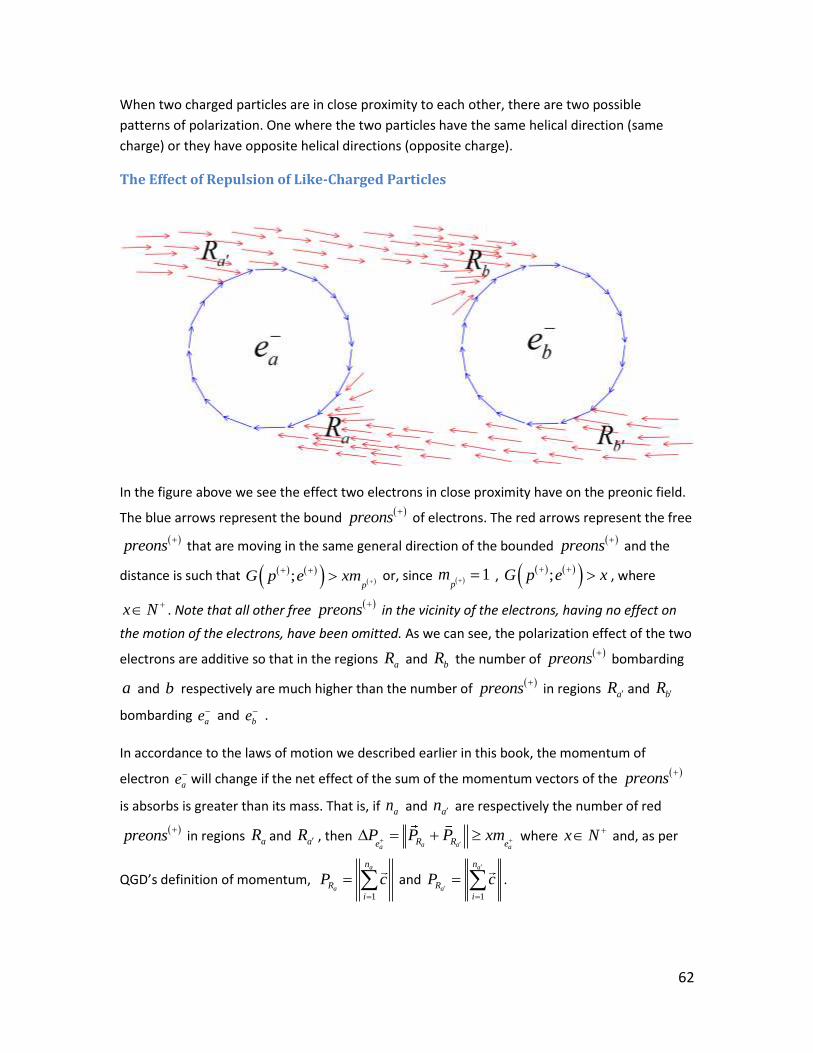
62
When two charged particles are in close proximity to each other, there are two possible
patterns of polarization. One where the two particles have the same helical direction (same
charge) or they have opposite helical directions (opposite charge).
The Effect of Repulsion of Like-Charged Particles
In the figure above we see the effect two electrons in close proximity have on the preonic field.
The blue arrows represent the bound
preons
of electrons. The red arrows represent the free
preons
that are moving in the same general direction of the bounded
preons
and the
distance is such that ;p
G p e xm
or, since 1
pm ,
;G p e x
, where
x N . Note that all other free
preons
in the vicinity of the electrons, having no effect on
the motion of the electrons, have been omitted. As we can see, the polarization effect of the two
electrons are additive so that in the regions aR and bR the number of
preons
bombarding
a and b respectively are much higher than the number of
preons
in regions aR and bR
bombarding ae and
be .
In accordance to the laws of motion we described earlier in this book, the momentum of
electron ae will change if the net effect of the sum of the momentum vectors of the
preons
is absorbs is greater than its mass. That is, if an and an are respectively the number of red
preons
in regions aR and aR , then
a aa aR Re e
P P P xm
where x N and, as per
QGD’s definition of momentum, 1
a
a
n
R
i
P c
and 1
a
a
n
R
i
P c
.
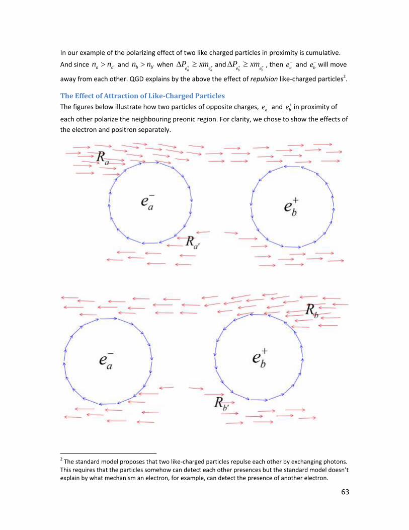
63
In our example of the polarizing effect of two like charged particles in proximity is cumulative.
And since a an n and b bn n when a ae e
P xm andb be e
P xm , then ae and
be will move
away from each other. QGD explains by the above the effect of repulsion like-charged particles2.
The Effect of Attraction of Like-Charged Particles
The figures below illustrate how two particles of opposite charges, ae and
be in proximity of
each other polarize the neighbouring preonic region. For clarity, we chose to show the effects of
the electron and positron separately.
2 The standard model proposes that two like-charged particles repulse each other by exchanging photons.
This requires that the particles somehow can detect each other presences but the standard model doesn’t explain by what mechanism an electron, for example, can detect the presence of another electron.

64
When an electron and a positron are in close proximity, the free
preons
between them are
directed towards the bottom so that a an n and b bn n . Hencea aR RP P
and
b bR RP P and, if
a aa aR Re e
P P P xm
and b bb b
R Re eP P P xm
, the
momentum ofae towards
be will change by will change by ae
P and the change in speed from
this state will be a
a
e
e
P
m
. Similarly, the speed of
be towards ae will be b
b
e
e
P
m
.
Also, as they become closer, the difference between an and an and that between bn and bn
will increase so that the rate of change in momentum, hence the acceleration, will increase. The
above explains the effect of repulsion between like-charged particles.
Now that we have explained the mechanism of the electromagnetic repulsion and attraction
effects, we will adopt the notation ;aH a b to represent the resultant momentum of the
preonic field resulting from the interaction effect on a from between a and b .
1
;Rm
a i
i
H a b c
where Rm is the number of
preons
polarized by a or b that hit a .
Electromagnetic Effects at Non-Fundamental Scales
At the non-fundamental scales, we must take into account the orientation of the electrons of
the structures. When the electrons are aligned, that is, they are moving in the same direction,
the polarization effect is cumulative. The gravitational interaction between the structure a and
any single free
preons
is given by 2
;2
i e
d dG a p n k
where
en is the number
of aligned electrons of the structure. Thus, by comparison to that of an electron, the distance at
within which we have significant gravitational interactions is e
n times greater. Or, from at a
comparable distance d , the gravitational interaction ise
n times greater.
If in the electron-electron interaction figure above we pivot the second electron by 180 degrees
around any diagonal drawn through its center, we obtain the configuration of an electron-
positron interaction. Now, in the figure, we assumed that that in an electron-positron
interaction that the particles are moving parallel to each other so they interact over distance. If
an electron and a positron would approach each other from opposite directions, the distance of
interaction would be too short to be significant. But things are different for bound electrons.
Since they move within closed trajectories, the distance between the aligned electrons of each
of the two structures can be maintained and as long as they are in proximity the gravitational
interactions between them will be significant.
65
The change in momentum resulting of an object a from the electromagnetic effects of
attraction or repulsion can be calculated using the same equations for the electron-electron and
electron-positron interactions by adding individual effects of the bounded
preons
which is
given by:
a aa R R aP P P xm
where x N and aRP is the resultant momentum of the free
preons
moving in direction of b , the second object, and
aRP
the resultant of those
moving away from it. So, if an number interaction
preons
is region aR and an , the number
of interacting
preons
in region aR then, since 1
a
a
n
R i
i
P c
and 1
a
a
n
R i
i
P c
,
1 1
a an n
a i i
i i
P c c
.
This explains why magnets can attract or repel each other even only electrons orbit the atoms at
their both magnetic poles. Or why a magnetic field, which two poles are generated by electrons
(not one with positrons and the other with electrons) can attract or repulse a beam of electrons
passing through it depending on the orientation of motion of the electrical current (electrons)
generating the magnetic field. It also explains why a strong magnetic field is generated when
passing an electrical current through a coil. The coil simply multiplies the number of surface
electrons that are aligned. All of these are phenomena that dominant physics theories can
describe but have yet to explain.
Electromagnetic Effect of Neutron Stars
Though the QGD model of the electromagnetic effect easily describes the interaction between
the bound
preons
within a neutron star and the neighbouring preonic field, which explains
its intense magnetic field, it will be most valuable when used to reinterpret existing
observational data and to interpret new observations. Such exercise would no doubt provide
significant information about the internal structure of these neutron stars.
Reverse Electromagnetic Effects of Attraction and Repulsion
We have seen above that, within a system consisting of two charged particles, if we change the
direction of the first particle by 180 degrees, the motion of its component
preons
relative to
the second particle will be reversed and, consequently, the first particle will interact with the
preonic field and the second particle as if it were its antiparticle. For example, in a system
consisting of two electrons, respectively tagged a and b , if we reverse the direction of the a
relative to b , then a will interact with b as if it were a positron.
Here is when it gets interesting. The effect of such change in the direction of a charged particle
not only holds for electrons and positrons, but for all charged particles. For instance, a proton
66
will then behave relative to the system as if it were an antiproton. So QGD predicts that two
protons will attract each other if they are moving in opposite direction.
Dark Matter Effect The subject of dark matter is probably one of the most intriguing questions in physics today.
Hardly a day goes by that doesn’t have someone claiming to possess a theory that explains dark
matter. Dark matter, or should I say the dark matter effect, is the subject of so much speculation
and theories (most of which are mutually exclusive) so that last thing I wanted to do was to add
to the noise.
Another problem, if you can call It that, is that QGD ‘s explanation of the dark matter effect is
too simple. It emerges naturally from its postulate. In fact, dark matter is at the very core of
quantum-geometry dynamics. You see, if quantum-geometry dynamics is correct, dark matter is
simply the macroscopic effect free
preons
. In other words, dark matter is made of free
preons
.
We have described
preons
has being the fundamental particle of matter in detail. Preons
form all other particles, including photons. Individually, they interact orders of magnitude more
weakly than the even the least massive photons, which is why no instruments can detect them
directly, but over sufficiently large regions of space, their collective mass is sufficient to
gravitationally interact with and affect the behavior of light and mass structures.
Dark matter, contrary to beliefs, is not dark. Dark, by definition is said of something that does
not emit light. QGD contends that dark matter has been observed and studied for nearly five
decades. You see, according to QGD, the only matter that existed in the primordial universe was
in the form of
preons
which were uniformly distributed throughout quantum-geometrical
space. We’ll call this state, the isotropic state, one in which nothing existed but dark matter.
During the isotropic state,
preons
, as a consequence of the attractive force acting between
them, started to form the simplest of all structures; the photons. And because
preons
were
distributed isotropically, so were these newly formed photons. These isotropically distributed
photons have been discovered in 1964 by Arno Penzias and Robert Wilson and called the comic
microwave background radiation.
A number of theories can satisfactorily describe physical phenomena and at the same time be
coherent, consistent with reality and mutually exclusive. Mutually exclusive theories can’t all be
right so the ultimate test, the only valid test of a theory is the predictions that it makes that are
original to it and can be verified experimentally or observationally. So what original predictions
can be drawn from QGD that can be tested in the real world? And how do can we know that
QGD is correct in its description of dark matter?
67
One of the most obvious implications of QGD is that sufficiently large regions of quantum-
geometrical space (minimally the size of a small galaxy) should contain the same amount of
preons
, or, since the
preons
is the fundamental unit of mass, have the same mass. That
is, 1 2R Rm m where 1R and 2R are regions of the same volume (the volume being defined
quantum-geometrically as the number of
preons
it contains).
Also, the mass of any regions of space is the sum of its free
preons
,
p
, and its bounded
preons
, p
, that is:
iii
R ppm m m where
ipm and
ipm are respectively the mass of
free
preons
which form dark matter, and bounded
preons
which for visible matter. To
give an example, a region which may appear to be empty must have the same mass as a region
of comparable size that is occupied by a galaxy or galaxies. The difference being that in the latter
a great number of
preons
are bound, hence concentrated, in material structures.
QGD Prediction From the above, since the intensity of the CMBR within a region of space must be proportional
to the number of free
preons
it contains and inversely proportional to the amount of visible
matter, the more visible matter a region contains, the weaker the CMBR should be. QGD
predicts an inverse correlation between the amount of visible matter and the intensity of the
CMBR. Thus, a sufficiently detailed CMBR map is expected to provide a snap shot of the
distribution of free
preons
or what scientists call dark matter.
Dark Matter and the Pioneer and Mercury Anomalies When taken into account, the dark matter in our own solar system provides a simple
explanation of the Pioneer anomalies and the perihelion precession of Mercury.
Supporting Observations Interested readers may find some the descriptions of supporting observations in the following
articles.
http://en.wikipedia.org/wiki/Low_surface_brightness_galaxy
http://en.wikipedia.org/wiki/VIRGOHI21
http://arxiv.org/abs/1010.5783
For who is willing to do a little bit of research, there is an enormous amount of observational
data that supports the QGD’s explanation and predictions about the dark matter effect.

68
The Structure of Nucleons and their Interactions As we have seen earlier in this book, what distinguishes particles from their antiparticles
is the direction of rotation of the helical path of their component preon
pairs. Since
all matter is made of preons
this implies that antimatter does not exist.
QGD suggest that nucleons are themselves composed of successive layers of orbiting
electrons or positrons kept at a specific distance thanks to the balance between the
gravity and the electromagnetic repulsion effects between them. According to this
model, because the net charge of the proton is equal to the charge of a positron, we can
assume that the proton has one more positron than it has electrons. That extra positron
would occupy the outer orbit of the proton.
Similarly, the neutron would have an equal number of electrons and positrons, which
would account for it neutral electric charge, but with electron occupying its outer orbit.
So when an electron collides with a proton, the electron and the outmost positron can
annihilate and produce a two photons and a neutron. Similarly, when a positron collides
with a neutron, the positron and the outmost positron can annihilate to produce one
antiproton and two photons.
In order to discuss the forces that bind particles into nucleons and nucleons into nuclei,
it will be useful at this point to introduce a system of notation that will describe
appropriately the structure of particles.
Particles will be represented by using the matrix form a
b
where the top expression
represents the structure’s outmost particle, the one that interacts with external
particles or structures. The bottom expression represents the core of the particle, which
doesn’t directly interact. The core is itself a composite particle.
For example, in the table below, e
n
represents the proton as a neutron at its core and
a positron on its outmost orbit and e
p
represents the neutron having an anti-proton at
its core and a positron on its outmost orbit.
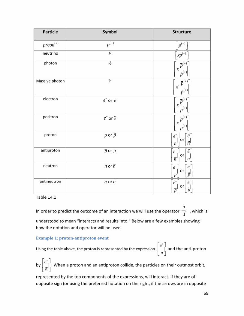
69
Particle
Symbol Structure
preon
p
p
neutrino v xp
photon
p
px
Massive photon
ixp
p
electron eor e
p
px
positron eor e
p
px
proton p or p e
n
ore
n
antiproton p or p e
n
orn
e
neutron n or n e
p
ore
p
antineutron n or n e
p
orp
e
Table 14.1
In order to predict the outcome of an interaction we will use the operator , which is
understood to mean “interacts and results into.” Below are a few examples showing
how the notation and operator will be used.
Example 1: proton-antiproton event
Using the table above, the proton is represented by the expression e
n
and the anti-proton
by e
n
. When a proton and an antiproton collide, the particles on their outmost orbit,
represented by the top components of the expressions, will interact. If they are of
opposite sign (or using the preferred notation on the right, if the arrows are in opposite

70
directions) then the components they will annihilate into their fundamental
components.
In our example, the interacting components of the proton and antiproton are an
electron and a positron which structures are respectively
p
px
and
p
px
so we
have:
2
px
p pn n x x n n
p
px
n
e
n nx
e p p
p
n
3
Once the operation is understood, we can simply write
2nn
ne
n
e
.
That is, the collision between a proton and an antiproton results in a neutron, an
antineutron and two photons (it can also produce four neutrinos instead of two
photons).
Example 2: Neutron-proton event.
The neutron-proton event is particularly important in that it helps explain the role
neutrons plays within in the atomic nucleus (this will be discussed under the topics of
particle decay and island of stability). The neutron-proton event is described as follows:
2
e
nn p
e
p
3 In our example we assume that x x
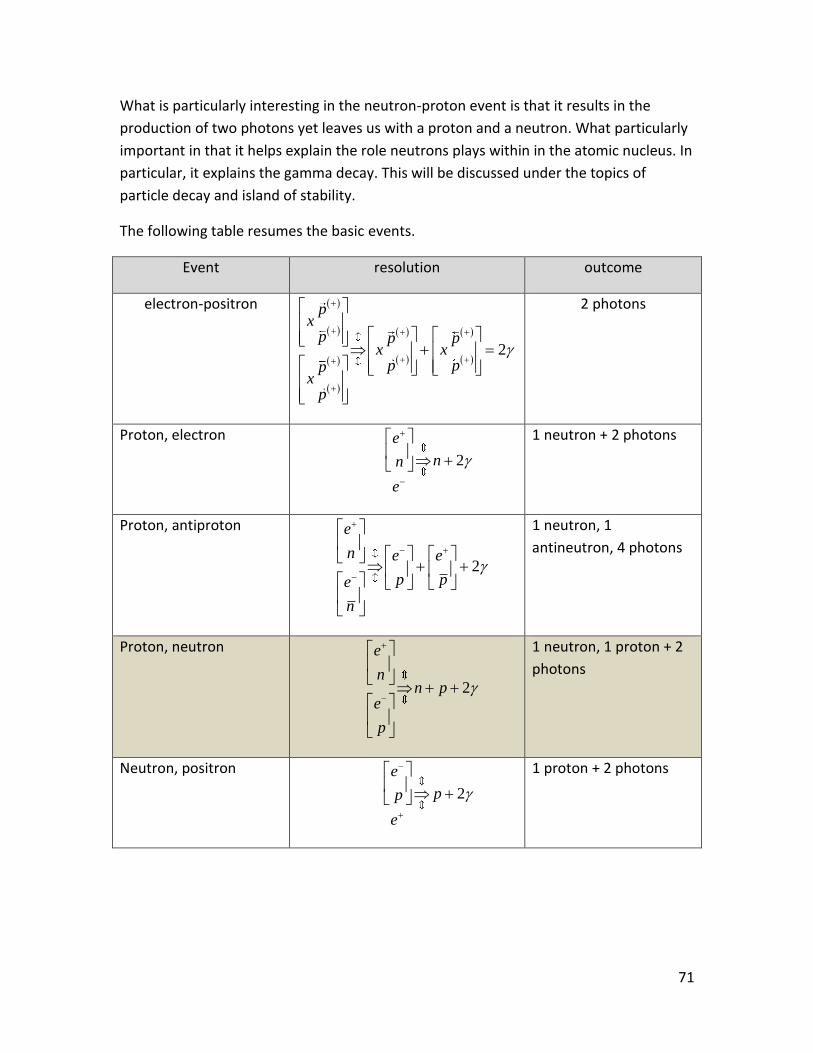
71
What is particularly interesting in the neutron-proton event is that it results in the
production of two photons yet leaves us with a proton and a neutron. What particularly
important in that it helps explain the role neutrons plays within in the atomic nucleus. In
particular, it explains the gamma decay. This will be discussed under the topics of
particle decay and island of stability.
The following table resumes the basic events.
Event resolution outcome
electron-positron
2
px
p px x
p
p
px
p
p
2 photons
Proton, electron
2
e
nn
e
1 neutron + 2 photons
Proton, antiproton
2
e
n e e
p
n
e p
1 neutron, 1
antineutron, 4 photons
Proton, neutron
2
e
nn p
e
p
1 neutron, 1 proton + 2
photons
Neutron, positron
2
e
pp
e
1 proton + 2 photons

72
Neutron, antineutron
2p
p
e
pp
e
1 proton + 1 antiproton+
2 photons
Antiproton, positron
4
e
nn
e
1 antineutron + 2
photons
Antiproton, antineutron
2n
n p
e
e
p
1 antineutron + 1
antiproton + 2 photons
Antineutron, electron
2
e
e
pp
1 antiproton + 2 photons
Table 14.2
It is understood that though the events respect the law of conservation, the law of
conservation alone does not explain the outcome of the events. A photon may have
enough mass to form an electron-positron pair, for example, but its quantum-geometric
structure forbids such an event. According to quantum-geometry dynamics, an electron-
positron pair can only be formed by two neutrinos or four gamma photons.
The Structure of the Atomic Nucleus
QGD admits the existence of only two fundamental forces, so the forces that bind
protons and neutrons into atomic nuclei must be result from the effects of these two
fundamental forces. This means that the strong interaction and the weak interaction,
which established theories considers to be the fundamental forces acting to bind
particles at the nuclear and fundamental scale must be effects of n-gravity and p-
gravity.
Using the notions we have developed throughout this book, let us examine the nucleus
of an atom and determine what forces are at play from the properties of it components.
For simplicity, we will examine the nucleus of a helium atom, which is the smallest
nucleus to have both protons and neutrons.
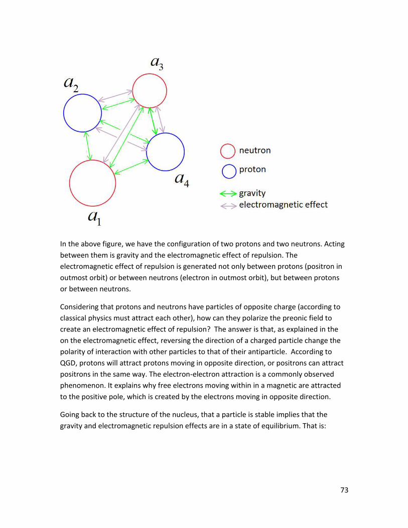
73
In the above figure, we have the configuration of two protons and two neutrons. Acting
between them is gravity and the electromagnetic effect of repulsion. The
electromagnetic effect of repulsion is generated not only between protons (positron in
outmost orbit) or between neutrons (electron in outmost orbit), but between protons
or between neutrons.
Considering that protons and neutrons have particles of opposite charge (according to
classical physics must attract each other), how can they polarize the preonic field to
create an electromagnetic effect of repulsion? The answer is that, as explained in the
on the electromagnetic effect, reversing the direction of a charged particle change the
polarity of interaction with other particles to that of their antiparticle. According to
QGD, protons will attract protons moving in opposite direction, or positrons can attract
positrons in the same way. The electron-electron attraction is a commonly observed
phenomenon. It explains why free electrons moving within in a magnetic are attracted
to the positive pole, which is created by the electrons moving in opposite direction.
Going back to the structure of the nucleus, that a particle is stable implies that the
gravity and electromagnetic repulsion effects are in a state of equilibrium. That is:

74
1 1
;ai
i
n A
i i j a
i j
c G a a m
where ian is the number of polarized
preons
absorbed by
ia , A is the number of nucleons contained in the nucleus (also called the mass number)
and where if i j then ; 0i jG a a . And since, at the nuclear and smaller scales, the
n-gravity component of the gravity effect becomes negligible4 then ;i ji j a aG a a m m k
and the above equation becomes 1 1
ai
i j i
n A
i a a a
i j
c m m k m
. It is also worth noting that
since nucleons have similar mass, iam is nearly constant. For the rest of this discussion,
we will substitute the constant sr for the term on the right so that the equation, which
from here on we will call the nuclear equilibrium equation, becomes
1 1
ai
i j
n A
i a a s
i j
c m m k r
.
The nuclear equilibrium equation implies that a nucleus or particle is stable when
1 1
ai
i j
n A
s i a a s
i j
r c m m k r
. That is, the difference in magnitude between the
gravitational and electromagnetic repulsion effects must be within the interval ...s sr r .
It follows that closer the combined effects of gravity and electromagnetic repulsion is to
zero, the more stable the nucleus or particle will be. Inversely, as the nuclear the closer
they are to the limits of the stability interval, the more instable the nucleus or particles
will become. And when the combined effects are outside the stability interval, the
nucleus or particle becomes highly unstable. Those are unlikely to be found in nature.
We will now discuss what happens when a nucleus or a particle becomes unstable and
the events such disequilibrium triggers that will bring it back to a state of equilibrium.
4 That, at nuclear and smaller scales, n-gravity is negligible explains the gravitational interactions between
nucleons are orders of magnitude greater than the gravitational interactions at large scales where the n-gravity component is important.

75
Gamma Decay
When 1 1
ai
i j
nA
a a i s
j i
m m k c F r
,
Here the gravitational interaction
surpasses the gravitational effect
sufficiently to pull neutrons and
protons towards each other
triggering neutron-proton events
(see figure on the left).
We learned earlier that a neutron-
proton event causes a proton to
change into a neutron and a neutron
to change into a proton. Using the
notation we introduced in this chapter, the neutron-proton event is described by
2
e
nn p
e
p
.
Such events, when occurring within an atom’s nucleus, would result in the emission of
two gamma photons5 while the atomic number and mass number of the atom remain
unchanged (although mass is changed by an amount equal to the masses of the emitted
photons).
The mass of the
interacting proton and
neutron is reduced by
2m(the mass of the
emitted photons) and this
in turn reduces the
gravitational interaction
within the nucleus,
5 Such events can also emit neutrinos or a combination of neutrinos and photon, but this will be discussed
in a more advanced treatise on quantum-geometry dynamics.
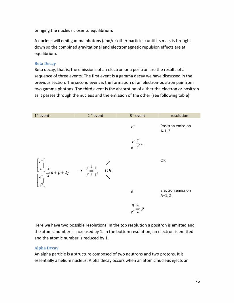
76
bringing the nucleus closer to equilibrium.
A nucleus will emit gamma photons (and/or other particles) until its mass is brought
down so the combined gravitational and electromagnetic repulsion effects are at
equilibrium.
Beta Decay
Beta decay, that is, the emissions of an electron or a positron are the results of a
sequence of three events. The first event is a gamma decay we have discussed in the
previous section. The second event is the formation of an electron-positron pair from
two gamma photons. The third event is the absorption of either the electron or positron
as it passes through the nucleus and the emission of the other (see following table).
1st event 2nd event 3rd event resolution
e
pn
e
Positron emission A-1, Z
2
e
nn p
e
p
e
e
OR
OR
e
np
e
Electron emission A+1, Z
Here we have two possible resolutions. In the top resolution a positron is emitted and
the atomic number is increased by 1. In the bottom resolution, an electron is emitted
and the atomic number is reduced by 1.
Alpha Decay
An alpha particle is a structure composed of two neutrons and two protons. It is
essentially a helium nucleus. Alpha decay occurs when an atomic nucleus ejects an
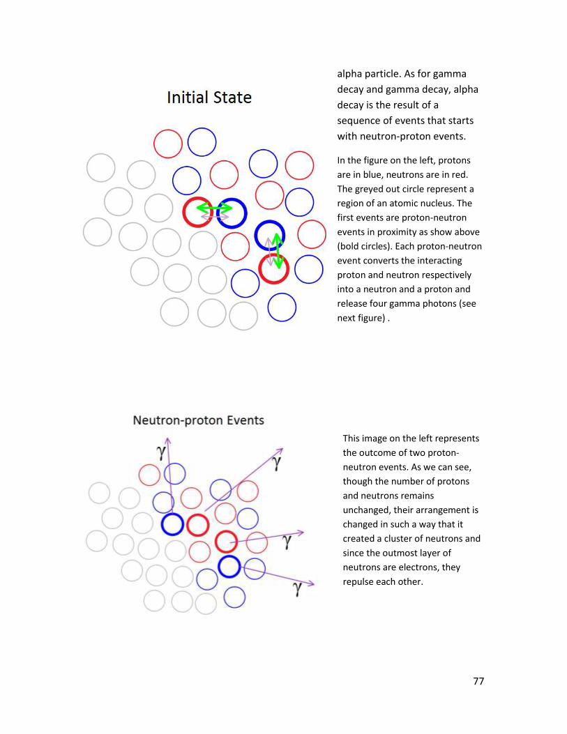
77
alpha particle. As for gamma
decay and gamma decay, alpha
decay is the result of a
sequence of events that starts
with neutron-proton events.
In the figure on the left, protons
are in blue, neutrons are in red.
The greyed out circle represent a
region of an atomic nucleus. The
first events are proton-neutron
events in proximity as show above
(bold circles). Each proton-neutron
event converts the interacting
proton and neutron respectively
into a neutron and a proton and
release four gamma photons (see
next figure) .
This image on the left represents
the outcome of two proton-
neutron events. As we can see,
though the number of protons
and neutrons remains
unchanged, their arrangement is
changed in such a way that it
created a cluster of neutrons and
since the outmost layer of
neutrons are electrons, they
repulse each other.
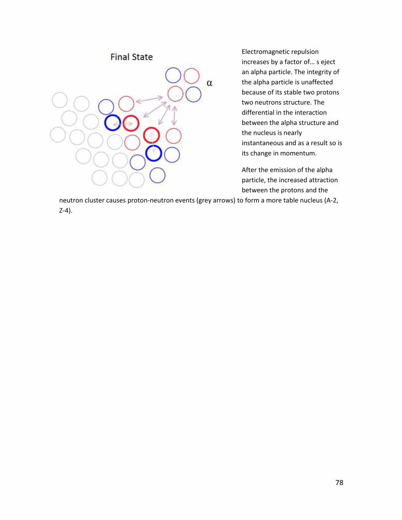
78
Electromagnetic repulsion
increases by a factor of… s eject
an alpha particle. The integrity of
the alpha particle is unaffected
because of its stable two protons
two neutrons structure. The
differential in the interaction
between the alpha structure and
the nucleus is nearly
instantaneous and as a result so is
its change in momentum.
After the emission of the alpha
particle, the increased attraction
between the protons and the
neutron cluster causes proton-neutron events (grey arrows) to form a more table nucleus (A-2,
Z-4).
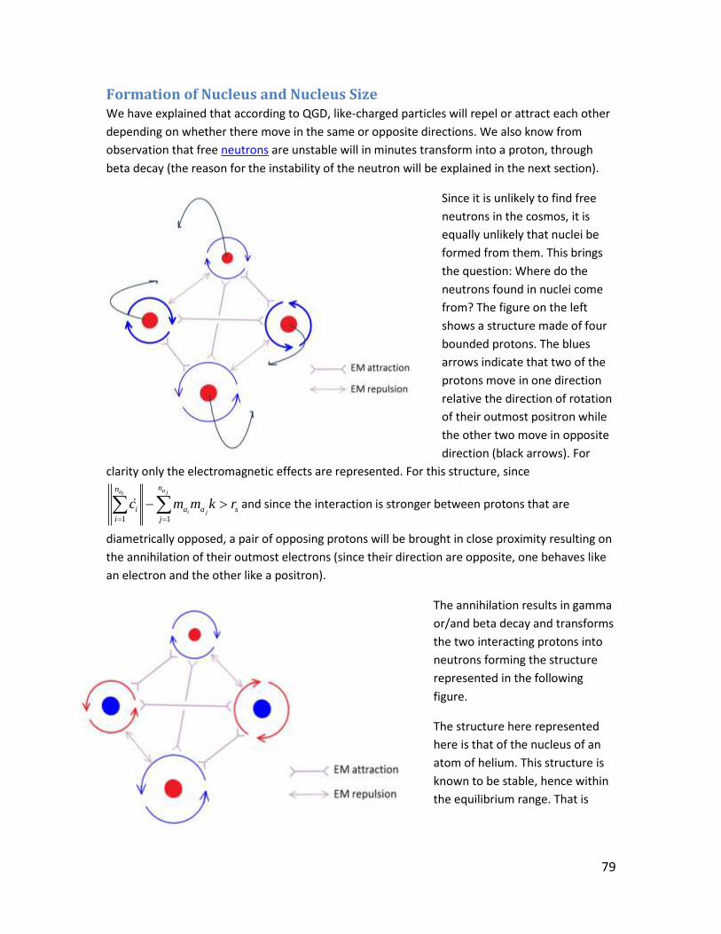
79
Formation of Nucleus and Nucleus Size We have explained that according to QGD, like-charged particles will repel or attract each other
depending on whether there move in the same or opposite directions. We also know from
observation that free neutrons are unstable will in minutes transform into a proton, through
beta decay (the reason for the instability of the neutron will be explained in the next section).
Since it is unlikely to find free
neutrons in the cosmos, it is
equally unlikely that nuclei be
formed from them. This brings
the question: Where do the
neutrons found in nuclei come
from? The figure on the left
shows a structure made of four
bounded protons. The blues
arrows indicate that two of the
protons move in one direction
relative the direction of rotation
of their outmost positron while
the other two move in opposite
direction (black arrows). For
clarity only the electromagnetic effects are represented. For this structure, since
1 1
aa ji
i j
nn
i a a s
i j
c m m k r
and since the interaction is stronger between protons that are
diametrically opposed, a pair of opposing protons will be brought in close proximity resulting on
the annihilation of their outmost electrons (since their direction are opposite, one behaves like
an electron and the other like a positron).
The annihilation results in gamma
or/and beta decay and transforms
the two interacting protons into
neutrons forming the structure
represented in the following
figure.
The structure here represented
here is that of the nucleus of an
atom of helium. This structure is
known to be stable, hence within
the equilibrium range. That is
80
1 1
aa ji
i j
nn
s i a a s
i j
r c m m k r
.
Explanation of Free Neutron Instability and Proton Stability
The instability of the neutron is easily explained when we apply the equilibrium
equation to the neutron’s components.
We know the proton is highly stable, that is1 1
aa ji
i j
nn
s i a a s
i j
r c m m k r
and
1 1
0aa ji
i j
nn
i a a
i j
c m m k
. There are two ways to obtain a neutron from a proton. The first
it by combining it with an electron which will it occupy the outmost orbit. The second it
to have it a positron interact with the electron in its outmost orbit so that they
annihilate. The annihilation transforms the proton into an neutron with an electron in
its outmost orbit.
In the first scenario, the net electromagnetic interaction of the neutron is smaller than
that of the proton (the particle becomes neutral), that is1
1 1
a ai in n
i i
i i
c c
. Also, since the
mass of the particle is the equal to the mass of the neutron plus the mass of the
positron, the gravitational interactions within the neutron is greater than the
gravitational interaction within the proton. That is:
1
1 1
a aj j
i j i j
n n
a a a a
j j
m m k m m k
. The
combination of the lower electromagnetic effect and higher gravitational effect is such
that 11
1 1
aa ji
i j
nn
s i a a
i j
r c m m k
. As a result, the component electrons and positrons (or
like charged particles moving in opposite directions) on neighbouring orbits will be
brought in close proximity resulting in the beta decay, the result of which is a proton
and the emission of an electron.
In the second scenario, we have again a reduction of the net electromagnetic
interaction, but a decrease in the gravitational interaction, that is 1
1 1
a ai in n
i i
i i
c c
and
1
1 1
a aj j
i j i j
n n
a a a a
j j
m m k m m k
. Here, neutron instability implies that

81
11
1 1 1 1
a aa a j ji i
i j i j
n nn n
i i a a a a
i i j j
c c m m k m m k
and we have 11
1 1
aa ji
i j
nn
s i a a
i j
r c m m k
,
which again leads to beta decay resulting in a proton and the emission an electron.
Not only models above explain why neutrons are unstable but they also provide an
explanation of why protons cannot not decay. The may interact with other particles
which would transform them into other particles, but, of itself, QGD predicts, they can
never decay.
Size and Stability of Nucleons and Nuclei
As we have seen, a nucleus is stable when the gravitational and electromagnetic effects
within it are in equilibrium. We also learned that when in a state of disequilibrium,
regulatory mechanisms of nuclear decay are triggered that until the nucleus achieves
the state of equilibrium.
It follows that the nuclear equilibrium equation may be used to predict the stability of
nuclei of any structure of size.
Also, though it exceeds the scope of this book, it can be shown that the equilibrium
equation can be applied to subnuclear composite particles and that the regulatory
mechanisms we have described in this chapter explain the stability or instability of
particles or their size. For instance, application of the equilibrium equation to protons
explains why they are the size they are and not larger or smaller.
82
Energy, Momentum and the Laws of Motion In this chapter we will show how quantum-geometry dynamics explains mass, energy, momentum.
As discussed in earlier chapters, quantum-geometry dynamics proposes that there be only two
fundamental particles: The
preon
, which dimensionalizes space, and the
preon
, the
fundamental particle of matter. What distinguishes quantum-geometry dynamics from dominant theories of fundamental physics, collectively known as the standard model, is that all properties of elementary particles are intrinsic. Essentially, this means that no additional particles and their properties are necessary to explain interactions not only at the fundamental scale but at all scales.
According to QGD, every particle or material structure is made of
preons
. That includes,
without exception, all particles we currently consider to be elementary. Electrons, positrons,
neutrinos and even photons are thus composed of
preons
.
preons
possess two intrinsic properties. The first is that they are strictly kinetic.
preons
are always in motion. Their speed is constant, hence their kinetic energy is constant and equal
to c . The speed of
preons
is constant whether they are free or bound within a composite
particle or structure. The constancy of the speed of
preons
is a direct consequence of the
quantum-geometrical structure of space.
preons
move by leaping from
preon
to
preon
. The preonic leap is fundamental unit of distance. Since there is no smaller distance
than the preonic leap, there is no faster motion than that of a
preon
.
The second intrinsic property of
preons
is that they interact with each other through p-
gravity, which is an attractive force acting between them. The p-gravity interaction between two
preons
is the fundamental unit of p-gravity or g .
Speed Redefined The reason this section is given the title Space-Matter-Light Interactions and not the more
common Matter-Light Interactions is that, according to QGD, quantum-geometrical space
interacts dynamically with matter and light in all optical phenomena. In this following sections
we will discuss optics, which will be found to be part of the more general subjects of preonics.
We will use the principles we have introduced earlier describe and explain the phenomena of
light absorption, light reflection and the photoelectric effect.
We will also examine the relation the fundamental forces that govern the motion of bodies
which determine how they interact with light. We will therefore reinterpret Newtonian laws of
motion and show how they are founded in fundamental reality. But first, we need to look at
QGD's definition of a concept central to all dynamics, that is, the notion of speed.

83
QGD definition of Speed The speed of an object is defined classically as a function of distance and time. But, as we have
seen in the chapter titled A Brief Discussion of the Concept of Time, quantum-geometry
dynamics considers time to be a purely relational concept. And since quantum-geometry
dynamics proposes that time is not physical aspect of reality it defines speed without time.
When we measure the speed of an object, we start counting the number of recurrences of a
particular state of a periodic reference system when the object is at a chosen initial point along
its trajectory and stop counting when it arrives at second, distinct point. The length of the
trajectory between the points divided by the number of recurrences counted (the ticks of a
clock) gives what we understand as the speed of the object. This method of measuring speed
which compares two quantities has so far defined speed for us, but what allows us to assume
that the number of ticks of a clock is a quantity that corresponds to a physical aspect reality?
As we have seen earlier in the book, clocks devices that count the recurrences of a particular
physical state of its inner mechanism. There is no relation whatsoever between what clocks
count and reality. Clock count the ticks of the clock, nothing else.
This assumption that time is physical is reinforced by the mathematical models we use which
represent space and time as geometrical dimensions but without making distinctions between
what exist only as a representation, that is, what is pure concept, from a representation of a
truly physical aspect of reality. The assumption that time is physical can be singled out as the
most misleading idea in the history physics; one that lead to paradoxes, singularities, infinities,
all of which creating severe inconsistencies in physical theories if not their complete collapse.
These problems alone justify abandoning the time-as-physical assumption and even the concept
of time itself. But how can we abandon the concept of time when so much of our physics
theories are based on it? How, for instance, does one define the essential notion of speed
without time?
Using the ideas introduced here we can define timeless speed as follow:
The speed a body a is the ratio of its momentum over its mass or aa
a
Pv
m where
1
am
a i
i
P c
where ic is the kinetic energy vector of a
preons
component of a which magnitude is
fundamental and equal to c . Therefore, the speed of an object is defined using two physical
quantities; the magnitude of the vector sum of the kinetic energy vectors of its component
preons
and its number of
preons
, its mass. We now have a working definition of speed
that is timeless, observer independent and natural.

84
Special cases:
As we have explained, the energy of any particle or structure is given by 1
am
a i
i
E c
and the
momentum by1
am
a i
i
P c
. In the special cases when the trajectories of the component
preons
of a are parallel,
1
a am m
i i
i i
c c
so that a aP E . In words, the momentum and
energy of such particles or structures are equal quantities (but not equal qualities).
This is evident for a single
preon
a where, since 1am , we have 1
1
1
a i
i
P c c c
.
Similarly, if a is a photon or a neutrino, we have a a aP E m c . Also, according to the QGD
definition of speed, aa
a
Pv
m , we have .a
a
a
m cv c
m This explains, amongst other things, the
constancy of the speed of light without invoking time or the mechanism of time dilation.
The equality a aP E also holds for any structure whose component
preons
have
trajectories are parallel regardless of its mass (see here). Such particles include the photon and
the neutrino, but theoretically, any particle or structure can achieve a speed equal to c if is
subjected to strong enough interactions. And since the maximum momentum any object can
have is equal to am c , its energy, the maximum speed is c .
QGD Speed versus Classical Speed
The speed of a body a is defined as 1
am
i
i
a
c
m
where am is the number of
preons
it
contains, its mass, and 1
am
i
i
c
is the magnitude of the vector sum of the momentum
vectors of its component preons
; its momentum . Thus speed is intrinsic quantity or,
in other words, it is independent of any frame of reference.
Since speed is an intrinsic property, the speeds of two distinct bodies are not additive.
On the other hand, distance is additive. For instance, consider two photons a and b
respectively located at positions 1s and 2s separated by distance d and moving towards
each other. Independent sequences of causally linked changes in positions will result in
85
bringing a and b to positions 1s and 2s . We can add the distance between 1s and 1s to
the distance between 2s and 2s then subtract the result from d to know the distance
separating the photons at 1s and 2s .
Also, since the classical measurement of the speed of a body really compares the
distance it travels while the distance travelled by a reference object (see On Measuring
the Immeasurable) then we can compare the sum of the distance travelled by the two
photons to the distance travelled by the distance travelled by either a or b . So the
classical speed being a function of distance, the distance travelled by two photons
would be twice the distance travelled by one photon, when the classical speed at which
the photons approach each other would be twice the classically defined speed of light.
Similarly, two photons moving in diametrically opposite directions would be receding at
from each other at a classical speed of twice the classically defined speed of light.
That said, since time is not a property of physical reality, classically defined speed,
including the speed of light, doesn’t have the physical meaning we attribute it.

86
Space-Matter Interactions
One of the fundamental assumptions of quantum-geometry dynamics is that space is not
continuous, but discrete, made of fundamental particles we call
preons
and that
spatial dimensions emerge from the repulsive interactions between them (n-gravity). This
has already been discussed in detail in previous articles (see here. here and here).
In previous articles, we have seen that the gravitational interaction between two particles
or material structures is described by the equation 2
;2
a b
d dG a b m m k
where
am and bm are respectively the masses of a bodies a and b measured in
preons
, k
is the proportionality constant relating between n-gravity and p-gravity and d is the
number of
preons
between a and b ; what we traditionally call distance. This
equation accounts for the contribution of the two fundamental forces that make up
gravity; that is, p-gravity and n-gravity. This is made more apparent when we know that
the equation is the simplification of 2
;2
a b a b
d dG a b km m m m
where the
components a bkm m and 2
2a b
d dm m
respectively represents the magnitudes of the p-
gravity force and the n-gravity force between a and b .
But while we have so far been using the equation 2
;2
a b
d dG a b m m k
to
calculate the gravitational interaction between two material particles or structure, it can
be used to calculate the interaction between matter and space itself. We know that p-
gravity only interacts between
preons
and that interaction is positive (attractive). But
preons
must exist in quantum-geometrical space, hence they exist as
/preon preon
pairs. The
preon
part of the
/preon preon
pair interacts with
the
preons
which form quantum-geometrical space through n-gravity. In effect,
because it has an effect opposite of p-gravity, we can think of the mass of
preons
as
being negative mass so that, for the component 2
2a b
d dm m
, the negative sign can be
interpreted as attributing a different meaning to the values am and bm which now
represent the number of
preons
a and b contain respectively. And since the am is the
87
mass of a , we can by analogy interpret am as being its negative masses. It follows that
all particles and material structures have both positive and negative masses.
From the above, we understand that in the p-gravity component of the equation we must
use the positive masses of, the number of
preons
they each contain. So, assuming that
the region b contains no
preons
, then 0bm and 0a bkm m . For the second
component of the equation, am and bm represent the negative masses of a and b , that
is, the number of
preons
pairing with
preons
or am and the number of
preons
in
the region b or bm . It follows that the force acting between an object a and an empty
region of quantum-geometrical space b is given by 2
;2
a b
d dG a b m m
. This
explains that, for an object to change direction, it must overcome the force exerted by
space itself. Resolving the equation for a change equal to one unit of distance in one
given direction, that is where 1bm and 1d , the n-gravity that must be overcome by a
is ; aG a b m .
Note about the Distinction between Mathematical and Physical
Meanings
QGD shows that mathematical symbols also have specific physical meaning. The
negative sign in the equation for gravitational equation implies that the masses following
it are negative masses. The equal sign in the equation E mc derived from the axiom set
of QGD does not represent the equivalence between mass and energy, but proportionality
relation between them.
The same holds true for mathematical operations. QGD allows only for integer values of
discrete quantities. That means that when we refer to division we mean the Euclidean
division since, as we will be exemplified below, the quotient and remainder of the
Euclidean division take different physical meaning.
The distinction between the mathematical and physical meanings is essential, not only for
quantum-geometry dynamics, but for any theory of physics. In fact, much if not all of the
problems with the interpretations of mathematical models of physical phenomena come
from having lacked to make the necessary distinction.
Position, Speed and Trajectories The laws of motion we have explained earlier can be used to calculate and predict the position,
speed and trajectory of an object from any initial state.

88
Let’s consider the simple case of an object b interacting gravitationally with an object a . As we
will understand from QGD’s description of the second law of motion, the only allowable changes
in momentum must be a multiple integer of its mass. That is,bbP xm where x N . This
implies that changes in momentum of an object b due to gravitational interactions occur at
positions that are at distances from the center of gravity of a such that
;b b bP G a b P xm where x N . We will call these positions transitional positions.
The spacing between the transitional positions along the trajectory of b depends on its mass.
The greater bm , the closer the transitory positions will be. Based on the QGD gravitational
interaction equation, 2
;2
a b
d dG a b m m k
, we see that the spacing between the
transitional positions is approximately proportional to the square of the distance between b
and a (see figure below).
Gravity induced
changes in
momentum occur at
transitional positions
are always equal to
bm which
corresponds to
changes in speed
that are equal to
b b
b
P m
m
or 1b
b
P
m .
It follows that the
speed of b between
two subsequent
transitional positions
ip and 1ip is
constant and equal
to /b i
b
P
m.
The momentum vector
providing both
direction and the
speed until it reaches
the next transitional
89
position, the previous or subsequent locations of b can be calculated from an arbitrarily chosen
initial position ip . It is important to remember that classical time being a notion that has no
physical meaning the distance b travels is relative not to the mathematical dimension of time
but relative to a chosen number of
preon
leaps of any given
preon
chosen as reference.
The time reference is therefore replaced by a distance reference. For example, we do not talk
about the distance an object b travels over n units of time, but rather the distance it travels will
over l
preon
leaps. That is,bv
d lc
where d is the distance travelled, bv the speed of b , l
the number of leaps and c the momentum of
preon
, which is also equal to its speed. Note
that the although the reference we have used here plays a role similar to that of the classical
notion of time has played in physics, it differs from it in that is based on a fundamental aspect of
physical reality; the
preon
leap which is the fundamental unit of distance. Thus, a fourth
dimension, even a conceptual one, is unnecessary. Reality can be fully described without the
concept of time or the purely mathematical dimension of time.
Application at the Newtonian Scale As we have seen above, the QGD laws of motion allows us to know the momentum, speed,
direction at any position along the trajectory of a body. To better illustrate the law of motion,
we will consider the classic example of a body for which /00
bP , that is, b is a free falling
body (see figure).
Since /0/ b bb i
P P im , the change in momentum between two transitional positions qp and
rp is equal to br q m , and total acceleration is equal to r q . But since the distance
between two transitional positions is proportional to the difference between the squares of
their distances from the center of gravity of a , if we set qp at the center of gravity of a then
the change in momentum between qp and rp is given by
2 2
2 2
q q r rb a b a b
d d d drm m m k m m k
and since 0qd
2 2
2 2
r r r rb a b a b a b
d d d drm m m k m m k m m
, the speed at qp is equal to
2
2
r rr a
d dv r m
. Thus the rate acceleration of a body is proportional to the mass of a
(the body towards which it is accelerated) and to the square of the distance of between its initial
position and the center of gravity of a , but is independent of the mass of b , which explains why
two bodies will have the same acceleration regardless of their mass. This is consistent with

90
Newton’s law of gravity, which at the scale it is applied to, distances in leaps are large enough so
that2 2
2 2
r r rd d d . Newton’s law of gravity emerges naturally from the principles of QGD and
corresponds to an approximation of its gravitational interaction equation.
The distance between two successive transitional positions is proportional to the difference
between the square of their distances from the center of gravity. This is also consistent with the
inverse square of the Newtonian equation (see figure).
As we have seen, according to QGD, an object interacting gravitationally doesn’t go through the
infinite number of infinitesimal speed increments implied by Newton’s gravity equation and
General Relativity. An object accelerates only at transitional positions. At non-fundamental
scales, the relative distance between transitional positions is small and the acceleration of an
object appears continuous. But the closer we get to the fundamental scale, the more evident it
becomes that the acceleration is discrete rather than continuous. This is consistent with
observation (see quantum leap).
Experimental Prediction
Based on the notions we have introduced in this section, the discrete acceleration of objects at
transitional positions should be observable. Data from a free fall experiment using an object
coupled with a precise enough accelerometer should show that the speed of an object changes
at transitional positions and that between them, their speed remain constant.
91
Laws of Motion and Optics
At this point some readers may wonder when this article will get on the subject of optics.
I'd like to reassure them that we haven't drifted from QGD optics and that this article is
rigorously on course.
The introduction of a new timeless definition of speed and an understanding of the
interaction between material objects and between matter and space are necessary
prerequisites to a quantum-geometrical description of the phenomenon of absorption and
reflection of light and the photoelectric effect. Also essential is the following discussion
about the laws of motion (which are given quantum-geometrical explanations).
First Law of Motion
If an object experiences no net force, then its velocity is constant: the object is either at
rest (if its velocity is zero), or it moves in a straight line with constant speed (if its
velocity is nonzero).
In quantum-geometrical terms the first law becomes:
If the magnitude of the vector sum of all the interactions with object a is null, then its
momentum, hence its speed, will be constant. Expressed in mathematical terms the first
law of motion express becomes:
1
; 0 0x
a
i
G a x P
This is a state in which that all external forces acting on a cancel each other. These
forces include the interactions with other particles and material structures, as described
by the QGD gravity equation, as well as the effect of quantum-geometrical space on it.
Thus an object moving at a constant velocity may be understood as one where the
external forces acting on it are in equilibrium.
Second Law of Motion
The acceleration of a body is parallel and directly proportional to the net force acting on
the body, is in the direction of the net force, and is inversely proportional to the mass m
of the body.
92
Expressed in QGD terms, Newton's second law of motion simply says that if
1
; 0x
i
G a x
then 0aP .
For gravitational interactions, the second law of motion can expressed as
1
;x
a
i
P G a x
.
To illustrate we'll examine the simplest case. That is, when all interactions acting on two
objects cancel each other except for the interaction between them . In this simple case
2
;2
a a b
d dP G a b m m k
. Since all QGD units are integers (and natural), we
know that changes in momentum from interactions will also be integer; that is a aP xm
where 0x N .
This is consistent with QGD when you consider that for a body of mass am to change
momentum in a particular direction, each of its component
preons
must overcome an
integer part of the n-gravity force exerted on it, as we have seen earlier.
Fundamentally, all motion imply that the component
preons
of an object leap from
preon
to
preon
so a fractional value would mean that
preons
could leap in
between
preons
. That, as quantum-geometrical space implies, is not possible since
nothing except the n-gravity field that keeps them apart and dimensionalize space and p-
gravity though which matter interacts can exist between
preons
.
Optics The theoretical interpretations of observations of the behaviour of light indicate that it possess
the mutually exclusive properties of the wave and the particle; a paradox that is known as the
particle/wave duality. That light may have wave properties was hypothesized following
observations of how light behaves in diffraction experiments, particularly in interference
experiments such as the double-slit experiment where light produces diffraction and
interference patterns that appear similar with diffraction patterns produced from observable
waves in nature (such as waves on the surface of liquid). The similarities between the diffraction
patterns are thought to imply that light may fundamentally be a wave.
Yet, some experiments, particularly those using a Talbot-Lau interferometer, have shown that
material structures such as protons, neutrons, atoms, and even very large molecules display
wavelike behaviour, that is, they display optical properties in the form of diffraction patterns.
93
That calls the question: Does the wavelike behavior of light imply that it is fundamentally a
wave? In order to answer that question, we need to understand what a wave is.
First, it is important to note that waves which we have observed and which inspired the wave
model of light actually emerge from the motion of discrete structures; the motion of molecules
of air or the molecules of water, for example. Thus the mathematical representation we call
wave function models the motion and distribution of discrete particles that constitute a medium
and describes the absorption and transfer of perturbation energy to other molecules of the
medium, which create the waves which will eventually restore the state of equilibrium that
existed prior to the perturbation (as when a stone is thrown in a pond, causing the displacement
of water molecules).
Thus waves emerge from the interactions between discrete particles. That brings the questions:
Is there really a wave-particle duality? Considering the above the answer is obviously "no."
Waves can be understood as the change in distribution in space of particles under the influence
of a perturbation (kinetic energy) (and gravity for liquids submitted to Earth’s attraction). The
wave properties are emergent, thus they cannot be fundamental.
Consider this: When studied under a powerful microscope, waves disappear leaving nothing but
the motion of molecules. So would it make sense that we attribute to water molecules the
fundamental property of the wave? Of course not! So why do we attribute the fundamental
wave property to light? A property cannot at the same time be fundamental and emergent. And
if we’re going to use the wave model for light, then isn’t not possible that its wavelike behavior
is also emergent? Couldn’t waves emerge from the discrete interactions between photons and,
for instance, the material slits are cut into to create the familiar diffraction or interference
patterns? QGD’s answer to the question is unequivocally “yes.”
We will show that the diffraction and refractions patterns of particles, including that of photons,
are actually scattering patterns that can be fully explained in terms of gravitational interactions
between photons and the experimental apparatus. Therefore, diffraction experiments with
larger particles dot not show that they possess wave properties similar to that of light, but the
opposite. That is, light shares the discrete structures of larger particles so that diffraction
patterns of light, too, emerge from the discrete gravitational interactions between photons and
the blocking material in which slits are cut. In other words, the diffraction and refraction
patterns can be fully explained without invoking any intrinsic or fundamental wave properties.
As a consequence, it can be argued that light is singularly corpuscular and the diffraction
patterns and interference patterns are simply scattering patterns of discrete particles caused by
gravitational interactions and the structure of quantum-geometrical space.
QGD proposes that all that is not space must be made of
preons
. That includes all particles
we currently believe to be elementary, even photons. QGD also proposes that energy is an
intrinsic property of
preons
which is their kinetic energy. The mass of a particle or material

94
structure is then equal to the number of
preons
it contains and its energy simply its number
of
preons
multiplied by c, their intrinsic kinetic energy. That is a aE m c .
Note that unlike Einstein's interpretation, E=mc is not an equivalence equation, but a
proportionality equation. In QGD, energy is an intrinsic property of matter and so cannot exist
without it. So energy can never be converted into matter nor matter be converted into energy.
Thus nuclear reactions are not events in which matter is converted into energy, but ones in which
bound particles are separated and carry with them their momentums.
Imagine two massive spheres in space, in absence of gravity, each equal in mass and moving at
high speed but attached by a string forcing them to orbit each other. Imagine that the system
consisting of orbiting spheres, taken as a whole, is at rest. Then, the momentum of the system is
equal to zero. Now, imagine that we suddenly cut the string. Taken as a whole, the energy of the
system does not change, but the spheres now move freely. The energy of each sphere hasn't
changed, but the sphere being free, they carry with them their momentum. Now, can we
conclude that part of the mass of the spheres changed into energy?
No, since they number of
preons
that compose them is unchanged. And since we know that
energy is an intrinsic property of
preons
, the energy of the sphere hasn't changed either.
This in essence is what happens in a nuclear reaction. Photons and other particles composing the
nuclear material which are bounded into a structure become free as a result of a nuclear
reaction and carry with them their momentum (in the special cases of photons and neutrinos, the
momentum is equal to the energy). The number of
preons
of a system is unchanged by
nuclear reactions, so mass and energy do not change either. The only difference is that
previously bounded particles are now free to interact with other systems, imparting them with
their momentums.
Now back to our subject; the singularity of light.
When distance is very short, as when light passes through a physical medium or comes very
close to it, applying the QGD motion equation shows that the interaction between photons and
the matter of the apparatus produces diffraction patterns identical to those observed in
diffraction experiments.
Consider the simple apparatus
shown on the left in which
light from a single source
passes near a massive
structure and hits the screen.
Using the equations for
gravitational interaction and

95
motion through quantum-geometrical space we introduced earlier we have:
;P P G a so that where ;G a xm , x N . The change in the momentum
component in direction of a must satisfy the equation ;aP G a xm and , the
angle of deflection, must then satisfy the equation ;G a xm
c c
. Only the angles of
deflection that satisfy this relation last equation are allowed.
If a photon passes close enough to a massive structure a , then it will change direction at
transitional positions. That is, at distances such that ;G a xm . So, the greater the
mass, the greater the gap between the allowable angles of deflection. It follows that a beam of
composite light passing in proximity of a massive object will have its more massive photons
deflected more than its less massive photons. Hence, gravity will act as a prism; separating
photons according to their masses (classically associated to their frequencies).
The dark band in fringe patterns observed in diffraction experiments correspond to forbidden
changes in directional momentum (the actual momentum of photons never changes). That is,
since P xm the dark bands corresponds to distances such that ;G a xm .
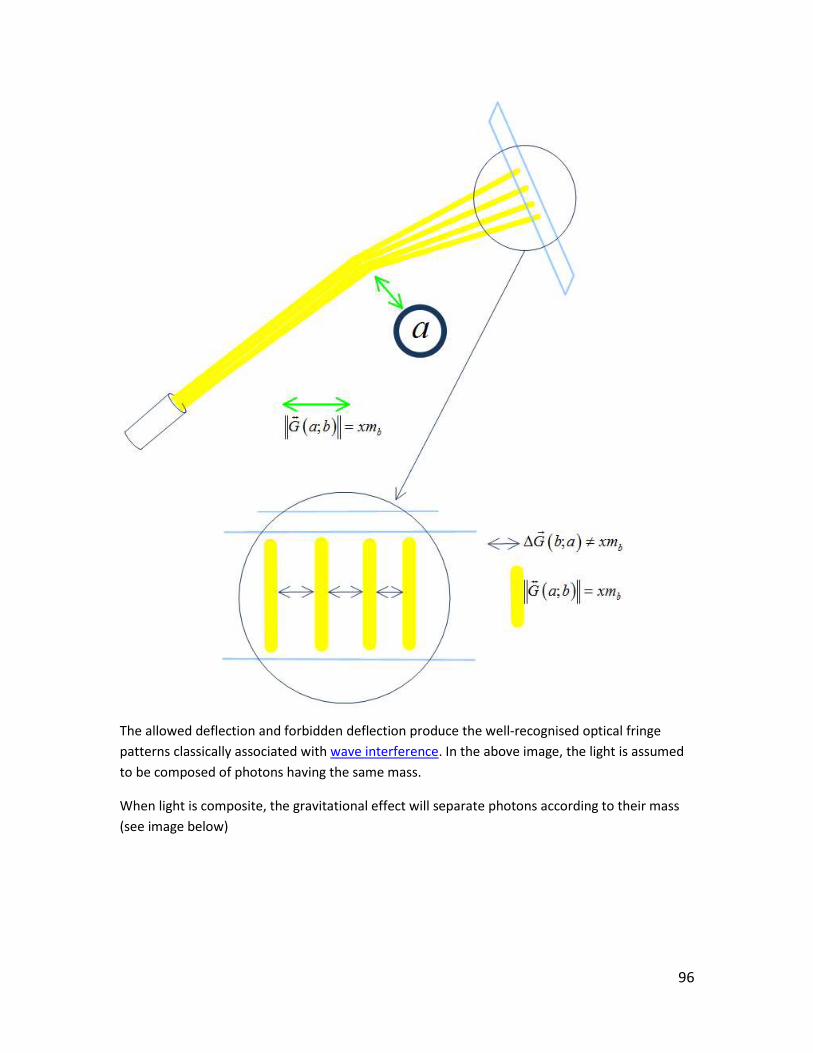
96
The allowed deflection and forbidden deflection produce the well-recognised optical fringe
patterns classically associated with wave interference. In the above image, the light is assumed
to be composed of photons having the same mass.
When light is composite, the gravitational effect will separate photons according to their mass
(see image below)

97
As you can see, the diffraction
patterns are produced using
only the QGD particle model
of light composed of photons
having mass.
The fringe patterns produced
in single or double slit
experiments are also fully
explained using QGD optics.
We have shown in this section
that gravity affect light the
way lenses or transparent
mediums do. We will now
show that gravitational lensing
and optical lensing are essentially one and the same phenomenon.
Refraction of Light In the previous section, we examined how photons interacting with matter can create the
diffraction patterns current physics associates with wave interference. It was shown that this
behavior of light can be fully explained using the QGD purely corpuscular model of light.
1. Photons are singularly corpuscular (so no wave-particle duality necessary)
2. Photons are composite particles made of
preons
therefore
3. Photons have mass and that mass is equal to the number of
preons
that form it
4. Space is quantum-geometrical, that is, it has a discrete structure. Hence, to predict the deflection of the trajectory of a photon, all we need to do is calculate the
gravitational interaction between it and whatever matter it interacts so that
;P G a xm
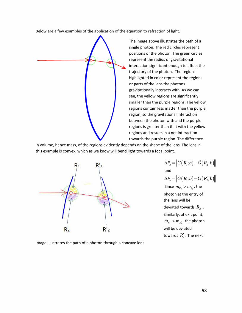
98
Below are a few examples of the application of the equation to refraction of light.
The image above illustrates the path of a
single photon. The red circles represent
positions of the photon. The green circles
represent the radius of gravitational
interaction significant enough to affect the
trajectory of the photon. The regions
highlighted in color represent the regions
or parts of the lens the photons
gravitationally interacts with. As we can
see, the yellow regions are significantly
smaller than the purple regions. The yellow
regions contain less matter than the purple
region, so the gravitational interaction
between the photon with and the purple
regions is greater than that with the yellow
regions and results in a net interaction
towards the purple region. The difference
in volume, hence mass, of the regions evidently depends on the shape of the lens. The lens in
this example is convex, which as we know will bend light towards a focal point.
1 2; ;bP G R b G R b
and
1 2; ;bP G R b G R b
Since 2 1R Rm m , the
photon at the entry of
the lens will be
deviated towards 2R .
Similarly, at exit point,
2 1R Rm m , the photon
will be deviated
towards 2R . The next
image illustrates the path of a photon through a concave lens.
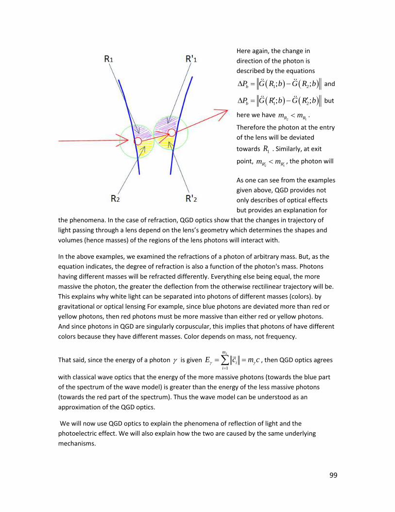
99
Here again, the change in
direction of the photon is
described by the equations
1 2; ;bP G R b G R b and
1 2; ;bP G R b G R b but
here we have 2 1R Rm m .
Therefore the photon at the entry
of the lens will be deviated
towards 1R . Similarly, at exit
point, 2 1R Rm m , the photon will
As one can see from the examples
given above, QGD provides not
only describes of optical effects
but provides an explanation for
the phenomena. In the case of refraction, QGD optics show that the changes in trajectory of
light passing through a lens depend on the lens’s geometry which determines the shapes and
volumes (hence masses) of the regions of the lens photons will interact with.
In the above examples, we examined the refractions of a photon of arbitrary mass. But, as the
equation indicates, the degree of refraction is also a function of the photon's mass. Photons
having different masses will be refracted differently. Everything else being equal, the more
massive the photon, the greater the deflection from the otherwise rectilinear trajectory will be.
This explains why white light can be separated into photons of different masses (colors). by
gravitational or optical lensing For example, since blue photons are deviated more than red or
yellow photons, then red photons must be more massive than either red or yellow photons.
And since photons in QGD are singularly corpuscular, this implies that photons of have different
colors because they have different masses. Color depends on mass, not frequency.
That said, since the energy of a photon is given 1
m
i
i
E c m c
, then QGD optics agrees
with classical wave optics that the energy of the more massive photons (towards the blue part
of the spectrum of the wave model) is greater than the energy of the less massive photons
(towards the red part of the spectrum). Thus the wave model can be understood as an
approximation of the QGD optics.
We will now use QGD optics to explain the phenomena of reflection of light and the
photoelectric effect. We will also explain how the two are caused by the same underlying
mechanisms.
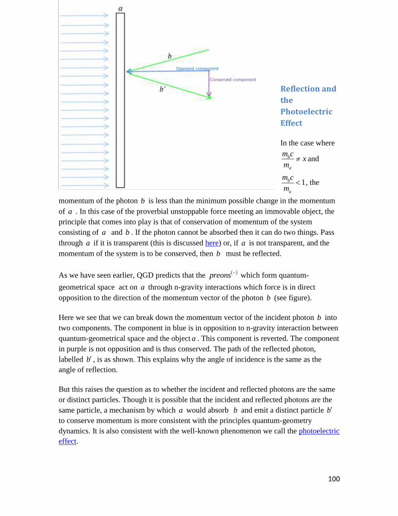
100
Reflection and
the
Photoelectric
Effect
In the case where
b
a
m cx
m and
1b
a
m c
m , the
momentum of the photon b is less than the minimum possible change in the momentum
of a . In this case of the proverbial unstoppable force meeting an immovable object, the
principle that comes into play is that of conservation of momentum of the system
consisting of a and b . If the photon cannot be absorbed then it can do two things. Pass
through a if it is transparent (this is discussed here) or, if a is not transparent, and the
momentum of the system is to be conserved, then b must be reflected.
As we have seen earlier, QGD predicts that the
preons
which form quantum-
geometrical space act on a through n-gravity interactions which force is in direct
opposition to the direction of the momentum vector of the photon b (see figure).
Here we see that we can break down the momentum vector of the incident photon b into
two components. The component in blue is in opposition to n-gravity interaction between
quantum-geometrical space and the object a . This component is reverted. The component
in purple is not opposition and is thus conserved. The path of the reflected photon,
labelled b , is as shown. This explains why the angle of incidence is the same as the
angle of reflection.
But this raises the question as to whether the incident and reflected photons are the same
or distinct particles. Though it is possible that the incident and reflected photons are the
same particle, a mechanism by which a would absorb b and emit a distinct particle b
to conserve momentum is more consistent with the principles quantum-geometry
dynamics. It is also consistent with the well-known phenomenon we call the photoelectric
effect.

101
Now, in the case where b
a
m cx
m and 1b
a
m c
m , the momentum of b is greater than the
minimum allowable change in momentum of a , but here the ratio b
a
m c
m being a non-
integer, a can only absorb b by emitting a particle b such that b bP r where br is the
remainder of the Euclidian division b
a
m c
m. It is here obvious here that br , the momentum
of b , if this particle is a photon, is also equal to its energy. The reflected photon will
have a lower momentum and then the incident photon (which we perceive has having a
different color). But b can be a particle other than a photon as long as its momentum is
equal to br .
For instance, instead of a photon a can emit an electron. Though the emitted electron
from the photoelectric effect may have a much greater mass than that of the incident
photon which caused its emission, it possesses the same momentum.
QGD Optical Transistor
Using the notions we have introduced, we see that the optical properties of a transparent
structure can be changed predictably by bombarding it with photons having momentum
that is equal to or greater than the structure's mass. Such photons will be absorbed by the
structure and will change its mass which in turn will change the allowed value for the
momentums of incident photons, thus allowing photons that pass through it to do so and
vice versa. QGD optics may be applied to create logical gates using only optical
components making the theoretical optical transistor a possibility.
Optics and Quantum Thermodynamics We will now apply the notions we introduced to explain how photons interact with matter and
the mechanisms by which it imparts what we call heat.
As we have seen, an electron can only absorb the part of a photon which momentum
corresponds to an integer multiple of it mass that is: e
m c xm , but whether the photon is
reemitted, scattered, reflected or refracted depends on the forces acting on the electron and in
the case of bounded electrons on whether the atom is orbiting is itself bounded or not.
Let us first consider the simple case of an unbounded hydrogen atom. The trajectory of the
electron is entirely described by the equations:
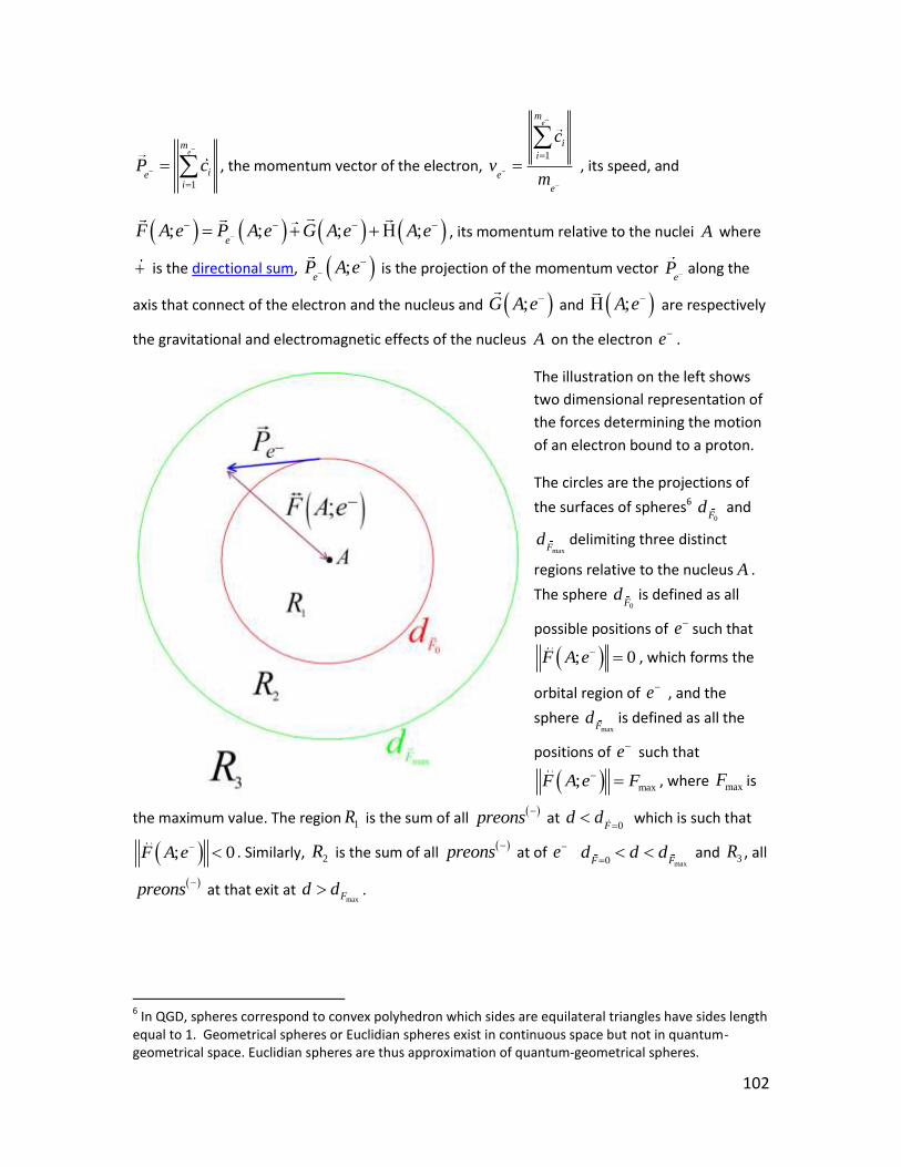
102
1
em
iei
P c
, the momentum vector of the electron, 1
em
i
i
e
e
c
vm
, its speed, and
; ; ; ;e
F A e P A e G A e A e
, its momentum relative to the nuclei A where
is the directional sum, ;e
P A e
is the projection of the momentum vector
eP along the
axis that connect of the electron and the nucleus and ;G A e and ;A e are respectively
the gravitational and electromagnetic effects of the nucleus A on the electron e .
The illustration on the left shows
two dimensional representation of
the forces determining the motion
of an electron bound to a proton.
The circles are the projections of
the surfaces of spheres6 0F
d and
maxFd delimiting three distinct
regions relative to the nucleus A .
The sphere 0F
d is defined as all
possible positions of e such that
; 0F A e , which forms the
orbital region of e , and the
sphere maxF
d is defined as all the
positions of e such that
max;F A e F , where maxF is
the maximum value. The region 1R is the sum of all
preons
at 0F
d d
which is such that
; 0F A e . Similarly, 2R is the sum of all
preons
at of e max0F F
d d d and 3R , all
preons
at that exit at
maxFd d .
6 In QGD, spheres correspond to convex polyhedron which sides are equilateral triangles have sides length
equal to 1. Geometrical spheres or Euclidian spheres exist in continuous space but not in quantum-geometrical space. Euclidian spheres are thus approximation of quantum-geometrical spheres.

103
From the equations describing ;G A eand ;A e we find that the magnitude of
;F A e increases positively as we move from 0F
d towards maxF
d at which distance it reaches
its maximum value of maxF , then (as ;A e becomes much less significant) it decreases
predictively as it follows closely the value of ;G A e.
Applying to QGD’s laws of motion to the simplest atomic system, the hydrogen atom, we can
see that given there no other acting forces than those we described in the example, the
electron’s trajectory will in the orbital region defined as all the
preons
forming the surface of
the sphere7 which distance to the nucleus is 0 0F
d
. In this state of equilibrium, the motion of
the electron relative nucleus is describe by the equation:
; ; ; 0e
P A e G A e A e
The electron will remain on the 0 0F
d
orbit indefinitely long as there are no other forces acts on
the system.
Note that for a stable hydrogen atom to be formed, we must have ; 0A e , which
negative value indicates is a repulsive force compensating the gravitational interaction and
allowing the existence of the atomic structure. If ; 0A e then we would have
; 0F A e and since the attractive component of the force is not compensated by a
repulsive effect, the electron will collide with the proton, resulting the production of a neutron
and photons. The neutron will then decay into a proton and an electron. Then, the
electromagnetic effect the new proton and new electron (which may then be recaptured) would
be ; 0A e ; that it, would form a stable atom. 8
The Effect of Photon/Electron Interaction on the Motion of Electrons In this section we will show how the motion an electron is strictly deterministic and that its
motion, after it interacts with a photon, can be calculated from a given initial state.
7 Since true spheres do not exist in quantum-geometrical space, what we call a sphere is a regular
polygon, which surface are made equilateral triangles having sides equal to one leap. The surface approaches that of a geometrical sphere as the distances two diametrically opposite summits increases. 8 Based on QGD’s model of the structure of particles, the electromagnetic effect between an electron and
a proton may be attractive or repulsive depending on the direction of the electron relative to motion of the components of the proton.
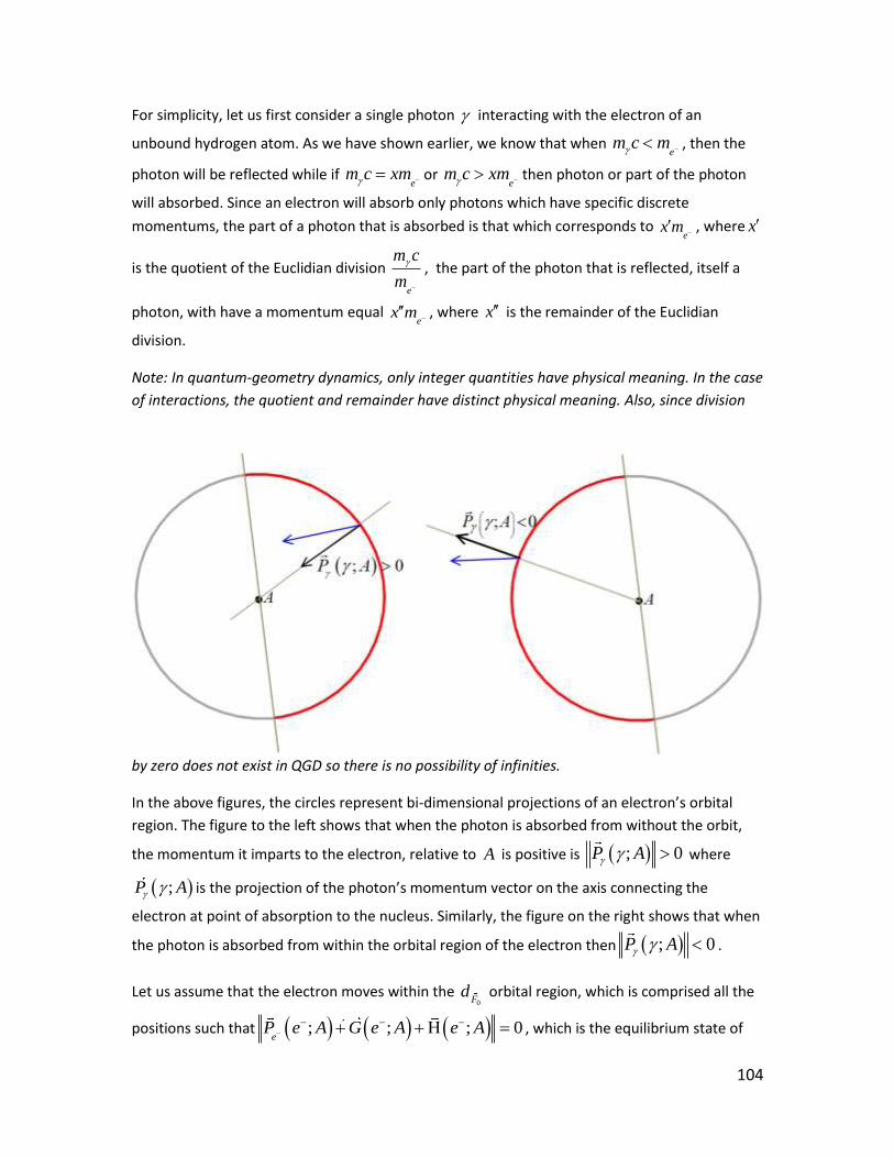
104
For simplicity, let us first consider a single photon interacting with the electron of an
unbound hydrogen atom. As we have shown earlier, we know that when e
m c m , then the
photon will be reflected while if e
m c xm or e
m c xm then photon or part of the photon
will absorbed. Since an electron will absorb only photons which have specific discrete
momentums, the part of a photon that is absorbed is that which corresponds to e
x m , where x
is the quotient of the Euclidian division
e
m c
m
, the part of the photon that is reflected, itself a
photon, with have a momentum equal e
x m , where x is the remainder of the Euclidian
division.
Note: In quantum-geometry dynamics, only integer quantities have physical meaning. In the case
of interactions, the quotient and remainder have distinct physical meaning. Also, since division
by zero does not exist in QGD so there is no possibility of infinities.
In the above figures, the circles represent bi-dimensional projections of an electron’s orbital
region. The figure to the left shows that when the photon is absorbed from without the orbit,
the momentum it imparts to the electron, relative to A is positive is ; 0P A where
;P A is the projection of the photon’s momentum vector on the axis connecting the
electron at point of absorption to the nucleus. Similarly, the figure on the right shows that when
the photon is absorbed from within the orbital region of the electron then ; 0P A .
Let us assume that the electron moves within the 0F
d orbital region, which is comprised all the
positions such that ; ; ; 0e
P e A G e A e A
, which is the equilibrium state of
105
the electron. When the electron absorbs a photon such thate
m c xm , the electron’s
momentum vector changes so that e e e
P P P P and consequently the interaction
between the electron and nucleus becomes ; ; ; ;e
P e A G e A e A P e A
.
Depending on whether ; 0P A or ; 0P A , the electron will move more distant or
closer orbital region.
If, for instance ; 0P A then, since ; ; ; 0e
P e A G e A e A
the
electron will move away from the proton. Then two things may happen, if
max;P A F then the electron will reach a region where ;G e A dominates and will
pull the electron back towards equilibrium, at which point it will reemit the absorbed photon .
In the cases where max;P A F , then ;G e Awill not dominate and cancel out the
outbound momentum so that the electron will be escape the atom.
Now, if ; 0P A then, since ; ; ; 0e
P e A G e A e A
, the electron will
move closer to the nucleus up to a region where ;e A will dominate and will push back the
electron towards the region of equilibrium. The electron will remit the absorbed photon which,
ife
m c xm , may be reemitted as x photons, each carrying momentumm
P cx
.
In all cases except where max;P A F , the electron will reemit the absorbed photon
and return to state of equilibrium in the orbital regions which, as we have seen earlier,
corresponds to all
preons
which distance from the nucleus is such that
; ; ; 0e
P e A G e A e A
.
When max;P A F the electron will be accelerated away from the atom at a rate
; ; ;e
e
e
P A e G A e A ev
m
and if no other forces act on the electron it
will achieve a maximum speed ofe
e
e
Pv
m
. This is the fundamental mechanism responsible
for the photoelectric effect and photovoltaic effects. Also note that we have only considered the
simple case where an electron absorbs one photon and either going back to the state of
106
equilibrium by reemitting it or escaping the atom if the momentum imparted by the absorbed
photon is sufficient. It is however possible for an electron to absorb two or more photons, either
simultaneously or successively. It such case, we would need to consider the effect combined
momentums of the photons.
The mass of the electron which escapes its atom is 1 0e e
m m m where 0e
m is the initial
mass of electron and m is the mass of the absorbed photon. Since the mass of the electron is
greater, then so will be the minimum momentum of absorbable photons. A photon can be
absorbed by 1e only if1e
m c xm where x N .
Also, for the electron is that of an atom that is bounded into a structure a and aP m , and
maxP F , then the photon cannot impart its momentum to the structure, so though it may
be absorbed by an electron. The resolution of the interaction requires that the photon absorbed
by the atomic electron be reemitted, which will restore the equilibrium.
107
Atoms Composed of Several Nucleons and Electrons
To describe how several electrons occupy different orbital regions of an atom, in addition to the
gravitational and electromagnetic interactions between electrons and the nucleus, we must take
into account these effects between the electrons. The equations describing the orbital regions
of an atom populated by n electrons is a set consisting of the n equations of the form
1, 1,
1, 1 1, 1
; ; ; ; ; ; ; 0i
i n i n
i i i j i i jej i j i
P e A G e A G e e A e A H e e A
,
where 1 i n and the expressions 1,
1, 1
; ;i n
i j
j i
G e e A
and 1,
1, 1
; ;i n
i j
j i
P e e A
represent
respectively the projection along the ;ie A axis of the combined gravitational and
electromagnetic interactions between a particular electron ie and the other 1n electrons.
The number of electrons necessary for an atom to achieve equilibrium, what we understand as
stability, must then be equal to the maximum number of electrons for which the all the
equations of the equation set holds. That is, if maxn n where maxn is the maximum number of
electrons that will satisfy the orbital regions equation set then, the adding an 1thn electron,
we must have
1
1 1 1 1 max
1
; ; ; ; ;n
n
n n n n jej
P e A G e A e A H e e A F
so that the 1th
n
electron will be ejected by the atom. Note that if the expression on the left was not smaller than
maxF , then there would be an 1thn orbital region which would contradict the initial
assumption that n is the maximum number of electrons for which the equation set is satisfied.
Also, it is possible that more than one electron move within the same orbital region as long as
the equation set is satisfied, but we have yet to see how the actual value of maxn determined.
It also follows that if the number of electrons is less then n electrons then
1, 1,
1, 1 1, 1
; ; ; ; ; ; ;i
i n i n
i i i j i i je ej i j i
P e A G e A G e e A e A H e e A xm
and
the atom will attract and capture electrons that come in proximity until it reaches equilibrium.
108
It follows that as the universe evolves, its atoms will gradually satisfy the equilibrium. This
implies that arrangements that do not satisfy the equilibrium equation set are not stable and
will necessarily transform into arrangements that do. This mechanism acts a form of natural
selection were only stable arrangements will persist.
For the hydrogen atom, it would appear that there are no solutions for 2n .
Proton-Particle Interactions
Since generally pm c m photons are not absorbed by protons, neutrons (or its component
particles) so photons are reflected by nucleons in accordance to the laws of optics we have
discussed earlier.
What is interesting here is that a photon reflected by a nucleus may interact with an electron
orbiting it; imparting its momentum the electron which will always add to the repulsive effects
between the nuclei and the electron.
Nucleon and Nucleus Equilibriums
The equilibrium equation set for atomic electrons are a special case of the equilibrium equation
sets that apply for all structures. All stable structures are described by solutions to similar
equilibrium equation sets. The motions of nucleons within a nucleus is subjected to the same
effects which determine the motion of bound electrons, the equilibrium states of a composite
nucleus is described by a set of equations having the form
; ; ; 0iA i i i i i iP A A G A A H A A where iA is any convex subset of nucleons of the
nucleus A and \i iA A A .
If a particle a with ia AP m collides with b , a nucleon of iA , it will be absorbed by it and, as
happens for bound electrons, if max;a i iP A A F then iA will escape iA that is, it will
result in the fission of A into iA and iA .
The structure of iA will be determined relation of aP and the forces binding the nucleons of iA .
iA and iA is a fission solution is that for which, ; ;\i a i ibF b A P A A and
max;a i iP A A F .
If ; ;\i a i ibF b A P A A and a bP m , then if max;aP b A F , then the fission
solution is iA b and \iA A b . That is, the nucleon b will be ejected.
Note that as before, a structure can only absorb a particle or part of a particle which momentum
is an integer multiple of its mass, that is ia AP xm where x N , so if

109
1i iA a Ax m P xm , then a part of a which will call a for which
ia AP xm will be
absorbed and the remainder will be emitted.
Note that the mechanisms described in this section explain not only fission and by fusion (when
max;a i iP A A F ) but all forms of nuclear decay. Nuclear decay, as all forms of decay, are
not probabilistic events but causal events which is the result of the interaction of a nuclei with a
particle. The stability of nuclei is then directly proportional to maxF .
Quantum Thermodynamics
According to QGD, what is classically referred to as the temperature of an object is not the
object’s temperature as such but the temperature of a region of quantum-geometrical space
which boundaries coincide with the boundaries of the object.
We have defined the heat and temperature of a region of quantum-geometrical space R
respectively as 1
Rn
R i
i
heat P
and 1
Rn
i
iR
R
P
tempVol
where iP is the momentum vector of the
thi particle of the from the set of Rn unbound particles contained within R and RVol is the
volume of R measured in
preons
. Thus we can define the temperature of an object a as
being the temperature of a region of quantum-geometrical space, aR ,which boundaries
coincide with the boundaries of a .
Theoretically, the lowest heat and temperature a can have, respectively 1
0R
a
n
R i
i
heat P
and 1 0
Ra
a
a
n
i
iR
R
P
tempVol
, correspond to a state where aR contains only a and in which the
electrons of a are at equilibrium. But since free
preons
, which account for most of the
matter in the universe, are distributed isotropically throughout quantum-geometrical space, we
must take into account the preonic density or p
density . Since R
pR
mdensity
Vol then
minR aa
heat R pVol density c and
mina
Ra
a
R p
temp pR
Vol density cdensity c
Vol
. That is,
the minimum heat and temperature of an object correspond to the heat and temperature of the
110
vacuum. It follows a value of zero for heat and temperature of aR is only possible for the very
special cases when
1aR
p
Voldensity
.
Thermodynamics of a Body
The temperature of an object a , which we have defined as the temperature of a region aR
which contours coincide with the contours of the object is 1
Ran
i
i
P
where iP is the momentum
vector of the thi of the aRn unbound particles within in aR . The heat and temperature of a will
change as the value aRn and this value will change as photons enter or exit aR and as photons
are absorbed or emitted by a . Thus 1
a a a a
s s
R R a a R Rn n emit abs abs emit where aemit are
the photons emitted by a , aabs are the photons it absorbs, aRabs are the photons absorbed
from outside aR , aRemit are the photons escaping aR and s and 1s are two successive
causality dependant states of aR .
So the variation in heat and temperature between two successive states s and 1s are
1
1
1 1
s sR Ra a
n n
s i j
i j
heat P P
and
1
1 1
1
s sR Ra a
a
n n
i j
i j
s
R
P P
tempVol
.
We can use the above definitions to describe what is classically called absorption, emission and
propagation of heat from and within an object, which in QGD are reinterpreted as the
absorption, emission and propagation of photons of a region which boundaries coincide with
the object. In order to do so, it may be simpler to divide the region aR containing the object
into sub-regionsiaR . The way aR should be divided depends on the shape a and direction and
number of photon sources outside aR .
Let us consider the simple example on the following page. The region containing the object a is
divided into sub-regions1aR ,
2aR and 3aR . The figure shows the causally linked states which a
will go through after the being bombarded simultaneously by a number of photons. We’ll
assume here that the electrons of a are at equilibrium, all have the same mass and are
components of the same element, and that the photons i have the same momentum such that
i em c m .

111
The photons that hit a sub-region are either absorbed, reflected or refracted. The maximum
number of photons that can be absorbed at a given state is equal to the number of photons
simultaneously hitting the sub-region minus the number electron which are at equilibrium. So
given there are enough photons that hit the sub-region simultaneously and the maximum
number of absorbed photons is reached, the rest of the photons will be either reflected or
refracted. The distribution of heat, which is really the distribution of photons, will follow a
pattern similar to that of our example.
When atom electrons of a structure absorb photons, they move away from their proton and
since the repulsive magnetic effect is proportional to their mass, the net force between the
atoms decreases. Given enough photons are absorbed, the increase in repulsive

112
electromagnetic effect will break the atom bonds and lead a change in the physical state of the
structure.
Note: In a sense, electrons “store” heat, which they release when the photons are reemitted. It
stores by lengthening the trajectories of the photons. So the slowing down of the photons
moving through a medium is caused by the lengthening of their trajectories in two different
ways. By the helical trajectories it adopts within the electron and by the trajectory of the
electron it becomes bound to. For two photons fired at the same time, one through vacuum and
the other through a medium, the difference between the distances traveled by the two photons
will be equal to the lengthening of the second photon’s trajectory as it was absorbed and
remitted successively by the atomic electrons it interacted with. Thus structures store photons
temporarily by bounding them to electrons which trajectories they must follow. In essence, they
delay the passage of light.
Modes of Photon Absorption and Emission
Ife
m c xm , the equilibrium may be restored though the successive emissions of n less
massive photons instead of the single photon . This is possible only if 1
i
n
i
m m
so that
1i
n
ei
m c xm
and if 0
11
i
i
i em c x m
c
where
iem is the mass of the electron prior to the
emission of the thi photon. This type of restoration of equilibrium explains, for example, why
phosphorescent materials will absorb photons and emit less massive photons over a longer
period. Considering the rates at which a structure will absorb or emit photons, it will take n
times as many emission events to restore equilibrium through multiple photon emissions as it
would take if equilibrium was restored through single photon emissions. Thus phosphorescence
will occur when 1
i
n
ei
m c xm
and0
11
i
i
i em c x m
c
with n being the greatest when
1ix (which is the greatest duration of reemission.
We can also have the reverse effect when the electrons absorb several photons simultaneously
or successively before returning to equilibrium by emitting a single photon. Photons that are
absorbed simultaneously can be treated as if it were a single photon of equivalent resultant
momentum. If 1
i
n
i ei
m c xm
the electron can return to equilibrium by emitting a single
photon such that 1
i
n
i
i
m c m c
or, as in phosphorescent materials, can emit multiple
photons. The modes of absorption and emission of photons will vary depending on the structure
of the atom as described by its orbital region equation set.
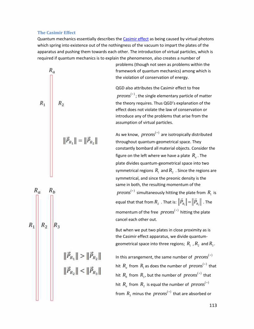
113
The Casimir Effect
Quantum mechanics essentially describes the Casimir effect as being caused by virtual photons
which spring into existence out of the nothingness of the vacuum to impart the plates of the
apparatus and pushing them towards each other. The introduction of virtual particles, which is
required if quantum mechanics is to explain the phenomenon, also creates a number of
problems (though not seen as problems within the
framework of quantum mechanics) among which is
the violation of conservation of energy.
QGD also attributes the Casimir effect to free
preons
; the single elementary particle of matter
the theory requires. Thus QGD’s explanation of the
effect does not violate the law of conservation or
introduce any of the problems that arise from the
assumption of virtual particles.
As we know,
preons
are isotropically distributed
throughout quantum-geometrical space. They
constantly bombard all material objects. Consider the
figure on the left where we have a plate aR . The
plate divides quantum-geometrical space into two
symmetrical regions 1R and 2R . Since the regions are
symmetrical, and since the preonic density is the
same in both, the resulting momentum of the
preons
simultaneously hitting the plate from 1R is
equal that that from 2R . That is: 1 2R RP P . The
momentum of the free
preons
hitting the plate
cancel each other out.
But when we put two plates in close proximity as is
the Casimir effect apparatus, we divide quantum-
geometrical space into three regions; 1R , 2R and 3R .
In this arrangement, the same number of
preons
hit aR from 1R as does the number of
preons
that
hit bR from 3R , but the number of
preons
that
hit aR from 2R is equal the number of
preons
from 3R minus the
preons
that are absorbed or

114
reflected by bR . Hence, if 1RP and
2RP are respectively the resultant momentum of the
preons
hitting aR from 1R and 2R , then we must have
1 2R RP P . And, if
1 2 aR R RP P xm , then net momentum imparted to aR will be a aR RP xm . In other
words, if aR was free, it would be pushed towards 2R and its speed will increase by
1 2
a
R R
R
P P
m
. Similarly, 3R would move towards 2R at 3 2
b
a
R R
R
R
P Pv
m
.
It is important to note that, If QGD is correct then the Casimir effect must affect all objects
which divides quantum-geometrical space asymmetrically. It follows that the Casimir effect
must affect objects at the cosmic scale as well; pushing cosmic structures towards each other
and contributing to the dark matter effect.
Redshift Effect and Cosmological Implications In a region of high photon density, the average mass of electrons will increase with the
absorption of photons having the required momentum and, from what we have shown, this in
turn increases the minimum momentum for successively absorbed photons. In conventional
terms, the emission and absorption lines of the region will be increasingly shifted towards the
blue region of the spectrum. This implies that the so-called redshifted electromagnetic
spectrum from a source is an indication that the source is at an earlier stage of evolution than
the reference source. Therefore, the redshift of a source is not a function of its speed or
distance, but of the average mass of its electrons, which itself depends on the relative stage of
evolution it is at. This implies that in order to determine the relative distance of a source, we
must compare its luminosity to the luminosity of the reference source and factor in the
magnitude of the spectrum shift which determines the relative age of the source at the time of
emission.
Since QGD implies that the universe evolved from an isotropic state, the formation of structures
at large scale will also be isotropic. Hence, the distribution of matter and the structures they
form will also be isotropic. This has the interesting implication that at a large scale, all regions
will undergo similar evolution at similar rate. What this means is that large scales objects at any
instantaneous state must have the same spectrum shift and that the only difference in spectrum
shift must be due the state of the source at the time of emission relative to the state of the
reference source at the moment of observation.
Since comparable source and reference source have reached in the present state of the universe
the same sate of evolution, then the magnitude of the observed redshift can is an indication of
the moment at which the source emitted the observed signal relative to the moment the
reference source emitted the reference signal. Thus the higher redshift, the more distant the
source may be. Thus the redshift, though it is not an indication of the relative speed of the
source, may be an indication of its distance. The relative distance of the source can be
115
calculated by comparing the difference in luminosity between the observed source and the
reference source and by taking into account the difference in luminosity between the stages of
evolution of the observed and reference sources.
Since the mass of electrons of a emission source increases exponentially as the source evolves,
that is 0
11
n
n
e em m
c
where n is the number of photons absorbed by
0em , the
momentum required for photons to be absorbed or emitted which is 0
11
n
n
em c xm
c
also
increases exponentially. Since de redshift is the difference between the masses of the emitted
photons from an element of the observed source b and the masses of photons from elements
of the reference source a , it follows that the observed redshift will increase exponentially. In
mathematical terms:
Since is a a
a em c x m and
b bb e
m c x m then the minimum redshift is when 1a bx x and
is given by a b
z m m or a be em m
zc
.
Since the average mass of the photons from a source directly depends directly on its stage of
evolution, we can attribute a numerical value it in the following manner.
A source is at stage s of its evolution if 0
11
s
s
e em m
c
where
sem is the minimum mass
of the electrons of a particular element of the source, 0e
m the mass of initial electrons.
Then the redshift between comparable sources is understood to be
s sa b
z m m where as and bs are respectively the stage of evolution at which the sources a
and b where at the momentum they emitted the photons we are comparing.
Distance Between Observed and Reference Sources of Photons
If ;d b a is the distance between a source of photons b and a reference source a is then
proportional to a bs s . From a bd s s it follows that the direction of a relative to b can be
determined by variations in b as s . If 0a bs s , then there is no increase in the redshift
effect other than what is attributable to the evolution of the sources and the distance between
a and b may be assumed to remain, hence the speed of a relative to b is zero ; 0a bv .
Similarly, if 0a bs s , then the increase in the redshift will be observed to is smaller than
that which can be attributed to the evolution of a and b and a is moving towards b .

116
And 0b as s then the observed increase in the redshift effect will be larger than which
that can be attributed to the evolution of a and b which implies that a is moving away from b
and ; 0a bv .
That said, since the rate at which a source evolves from one stage to next is not constant (it
depends on the density of free absorbable photons corresponding to each stage) then actual
distance can only be roughly approximated from the observed redshift. Distance can be better
approximated by comparing the luminosity of observed source to the reference source.
We will see later, that the only way to get the actual distance of an object is to measure the
gravitational interaction between the observed source and a reference object.
On Measuring the Immeasurable Key to our understanding of reality is our ability to measure certain physical properties of
objects such as mass, energy, speed, momentum, as well as quantify the forces acting between
them. But measurement experiments are designed based on how we model certain
fundamental aspects of reality. But how do we know if aspects of reality we consider
fundamental really are? And if not, what are we measuring when conducting a measurement
experiment designed to quantify such aspects? Can we even measure aspects of reality that are
truly fundamental?
To answer these questions, we will look at one of the most important measurement in physics;
that of the speed of light. The constant c which represents the speed of light is an essential
component of physics theories. One that is used in an important number of equations. It is
therefore no surprise that experiments have been perfected so as to make as precise
measurements of c as technology allows. But do these experiments really measure the speed of
light? And if not, what are they measuring?
Speed is classically defined as the ratio of the distance of displacement over time ord
twhere d
is the distance an object will travel during a time interval t , both of which expressed in
standardized but arbitrarily defined units. But QGD considers time to be non-physical and so
offers a definition of speed that does not make use of the concept of. We have seen that QGD
defines the speed of a body a as the ratio of its momentum over its mass or a
a
P
m with the
understanding that am is the number of
preons
contained by a and that its momentum is
defined as the resultant of the momentum vectors of each of its component
preons
or
117
1
am
i
i
c
where ic c all of which are expressed in fundamental units which by definition are
non-arbitrary and natural.
The speed of light corresponds to the speed of the photons that compose it. So using QGD’s
definition we find that the speed bv of a photon b is given by 1
bm
i
i
b
b
c
vm
and since all the
momentum vectors of the component
preons
of b have the same trajectories,
1 1
b bm m
i i b
i i
c c m c
so that bb
b
m cv c
m . Note that
1
bm
i
i
c
is the energy of b so that for
photons, energy and momentum have the same numerical value.
It follows that light speed measurement experiments are designed to measure the “classical”
speed of light (for example, see the Fizeau-Foucault apparatus) and so must result in
measurements of c that differ from the fundamental speed of light as expressed by the QGD
equation. In fact, they don’t measure speed at all.
What light speed measurement experiments do is compare the distance a reference object
moving at a known classical speed (time dependant speed) travels while light travels a known
distance. Then using the classical definition speed, dividing the distance travelled by the
reference object by its known speed gives the time that elapsed during which light travelled the
known distance. Then, by dividing the reference distance travelled by light by the time elapsed,
we get the classical speed of light. So ultimately, what such light measurements experiments
provide are not measurements of the fundamental speed light, but the speed of light relative to
the speed of a reference object.
Though these experiments cannot measure the fundamental speed of light (which from here on
we’ll refer to as the absolute speed of light), dividing their measurement of speed of light by the
speed of the reference object eliminates the time variable and gives us the proper ratio of the
absolute speed light over the absolute speed of the reference object. That is, such experiments
are useful in that we get a correct estimate of the ratioa
c
v.
That said; no experiments will ever the measure absolute speed of light or, for that matter, the
absolute speed of any other object. Since the measured speed of light is relative to the speed of
the reference object, and vice versa, there is no way to isolate c or av from the ratioa
c
vso that
neither can be known. But what if we designed an experiment based, not on the classical
118
definition of speed, but on QGD’s definition; that is, design an experiment which aims to
measure the speed of light (or any object) against quantum-geometrical space.
Since the absolute speed of an object a can be understood as its speed against quantum-
geometrical space, it av can be calculated by comparing the distance it travels with the distance
traveled by reference free
preon
or a photon b using the relation a a
b
d v
d c so that a
a
b
dc v
d
. The problem here is that we can’t know av without first knowing c which requires that we
measure the speed of a
preon
or a photon. Now if a is a
preon
or photon then a bd d
so we get b
b
dc c
d or c c . It may appear that this statement is trivial, but what it means for
physics is that any experiment that will attempt to measure the speed of an object against
quantum-geometrical space will always come down to the physical tautology that the speed of
light is equal to the speed of light. Hence, motion against quantum-geometrical space cannot be
detected or measured. This is one of several reasons that explains the failure of the Michelson-
Morley’s and similar experiments that attempted to measure the speed of the Earth against the
aether (the Michelson-Morley experiment suffers from other interesting theoretical problems,
which we’ll discuss in the addendum at the end the present section).
Now, you would be justified to ask: if it is impossible to measure the absolute speed of an
object, hence impossible to detect quantum-geometrical space, how can we prove it exists?
How can we prove the existence of
preons
, which form quantum-geometrical space? How
can we prove the existence of n-gravity which is carried by
preons
and which with p-gravity
produces the effect of gravity? Ultimately, how can we know quantum-geometry dynamics is a
valid theory when we can’t test one of its defining axioms?
Though it is true that we will never be able to detect quantum-geometrical space, the
assumption of its existence allows QGD to provide descriptions and explanations of observable
phenomenon but, most importantly, to make unique predictions that can be tested at
observable scales of reality.
Other Immeasurables and the Experimental Method We have shown that all experiments that attempt to measure the absolute speed of light will be
tautological and since the knowing the absolute speed of light is essential to know the absolute
speed of any object, we find that it is impossible to measure their absolute speed as well. But
also tautological are experiments that will attempt to measure other fundamental aspects of
reality. For instance, we know that the absolute mass of an object is the number of
preons
it
contains, but an experiment which will attempt to measure this will require that we know the
119
mass of a single
preon
. And what is the mass of a
preons
? The mass of a
preon
is
equal to the mass of a
preon
.
Similarly, it can be shown that all experiments that aim to absolutely measure other aspects of
reality such as the absolute distance between two
preons
, the absolute magnitude of
gravitational interaction, etc., all are tautological. All follow the theorem.
Fundamental reality is the absolute limit of the experimental method.
What the theorem implies is that if something is truly fundamental; it cannot be absolutely
measured and/or observed. That is: any and all measurements are inherently relative.
Gravity and the Speed of Light Another immeasurable is the “speed” of gravity. Since gravity is predicted to be instantaneous,
according the QGD’s definition of speed, it doesn’t possess the property of speed. QGD
proposes that all objects in the Universe are gravitationally interacting with only the magnitude
in the interactions varying in accordance to the gravitational interaction equation. Changes in
the mass of two objects or changes in distance will instantly affect the magnitude of the
gravitational interaction between them. Instantaneity implies that there is no propagation and
that gravity has no speed. In other words, gravitational interactions simply exist. Since gravity
has no speed, QGD predicts that any experiment designed to measure the speed of propagation
of gravity is bound to fail.
But though we can’t measure instantaneity, we can design an experiment which takes
advantage of the fact that we can measure variations in the gravitational interaction to prove
instantaneity.
The experiment would require two spheres, a and b , in space, having large enough mass for
the gravitational interaction between them to be measurable.
Sphere a would contain a powerful explosive, a detonator and an accelerometer. Sphere b
would carry an accelerometer calibrated to match that of the sphere a and a data recording
device. The experiment would measure the acceleration of the spheres towards each other in
accordance to QGD’s law of gravity. The detonator, linked to the accelerometer of sphere a
would be set so that when it reaches a speed av (which speed can be used to calculate the
gravity and distance between the spheres), it would detonate the explosive. Note that the
structure of sphere a would need to allow for a non-symmetrical scattering of its fragments.
There two possible outcomes to this experiment:
If the gravitational interaction is instantaneous, then the rate of acceleration of the sphere b
would change instantaneously when it reaches the exact speed at which the detonation of first

120
sphere a occurs. So if av is the speed at which the detonation of sphere a is set to explode and
bv is the speed it reached when the rate of acceleration of b changes, then 0b av v .
But if, contrary to QGD’s prediction, gravity did propagate, then we would find that 0b av v .
This is an example of a unique prediction that is a consequence of the existence of quantum-
geometrical space.
Addendum: About the Michelson-Morley Attempt at Measuring the
Immeasurable One of the reasons the Michelson-Morley experiment was doomed to fail to detect the motion
of the Earth relative to the ether is that all experiments designed to measure the absolute
motion of an object are tautological. The other reason is that the possibility of detection of the
motion of the Earth against the ether was based on the wave model of light.
Because of their resemblance with wave interference patterns observed at the surface of a body
of water when waves produced by different sources intersect, it was assumed that fringe
patterns produced during double-slit experiments implied that light possessed wave-like
properties. The Michelson-Morley’s experiment was designed to observe of the specific
interference patterns the wave model of light predicted the experiment, if successful, would
produce. So though the Michelson-Morley experiment was designed to test the ether theory, it
may correctly be seen as a test of the wave model of light. So the failure to observe the
predicted interference patterns may be taken as a refutation of the wave-particle duality.
The null result of the Michelson-Morley experiment is consistent with QGD’s explanation that
the fringe patterns observed during double-slit experiments and other diffraction experiments
are not caused by wave interference, but are scattering patterns resulting from the interaction
between the corpuscular component of light, quantum-geometrical space, and the material
structure of the apparatus, principally, the material in which the slit are cut.
Conclusion
We have seen in this series how light-matter interactions can only be understood when taking
into account the effect of quantum-geometrical space on matter and light. And once we accept
that light, like all material structures, is made of
preons
, light-matter interactions are really
matter-space interactions. Thus since optical phenomena are special cases of matter-space
interactions, they are governed by the same general laws that govern the motion of all matter.
Contrary to classical space, quantum-geometrical space is not a passive medium in which
physical events and interactions occur, but an active component in all events and interactions.
The effects of quantum-geometrical space are as tangible as the effects of matter.

121
Finally, it is important to remember that the examples given in this illustrate specific
mechanisms which in nature do not act in isolation. The photons that compose the beam of light
that hits an object can be partly absorbed and/or reflected and/or refracted and/or diffracted all
at once depending on the properties of the matter they interact with.
The mechanisms we described also explain how the mass of photons change as they travel from
a distant source. Photons emitted by a star, for example, will lose mass which equates into loss
of momentum (or, since for photons momentum and energy are equal, less energy). This well-
known and observed phenomenon is called the redshift effect. The variation in the mass of
photons provides some indication of the distance from the source (the larger distance it travels
the more likely they are to interact with interstellar matter), but though there is a correlation
between the distance and the amplitude of the redshift effect, the correspondence is not
necessarily proportional.
122
Collision Physics at Our Scale and the Mechanics of Momentum
Transfer So far, we have discussed the dynamics of particles at the fundamental scale. We have shown,
for example, that the momentum of a particle a can only change by value equivalent to integer
multiple of its mass. That is: a aP m . So, an a photon b can impart momentum to an
electron if b aP xm where x N . If b aP m then the transfer of momentum is forbidden
and photon will be reflected. If b aP xm it will be absorbed entirely by the electron (all its
preons
will become part of the electron’s structure). And finally, if b aP xm , the electron
will absorb n
preons
from the photon where b
a
a
Pn m
m
and will an electron b such
that b
b b a
a
PP P m
m
and b bm m n and with momentum and energy equal to nc . 9
The above not only explains the absorption lines of an atom, but also the emission lines since
emitted photons must definite momentum (see spectral line).
The reader may wonder what the above has to do with collision physics at our scale. What the
law of motions at the fundamental scale got to do with the physics that govern how a baseball
will transfer momentum to a ball or how the balls of poll transfer momentum to each other?
We will show in the chapter that all physical phenomena are governed by the same forces and
effects and that the physics at our scale being observable consequence of fundamental
interactions and as such should be describable using the same equations as those used for
fundamental phenomena.
Baseball Physics A postulate of quantum-geometry dynamics is that space is fundamentally discrete (quantum-
geometrical, to be precise). Of course, proving this using our present technology may appear to
be beyond difficult especially if, as QGD suggests, the discreteness of space exists at a scale that
is orders of magnitude smaller than the Planck scale. The task of proving that space is made of
preons
may even be impossible because, if as discussed in On Measuring the Immeasurable,
fundamental reality lies beyond the limit of the observable. That said, in the same article I
9 The reader will remember that in the special case of photons and neutrinos, momentum is equal to energy so that
1 1
b bm m
b i i b
i i
P c c m c
where ic are the momentum vectors of the component preons(+) of b .

123
explain that though
preons
, which according to QGD is the discrete and fundamental unit of
space, and
preons
, its predicted fundamental unit of matter, must be unobservable, their
existence implies consequences and effects that must be observable at larger scales.
This implies that we already observed consequences of space and matter being quantum-
geometrical but only lacked the theory capable of recognize them. It then makes sense to re-
examine observations which, when interpreted by QGD, may provide proof of that space is
quantum-geometrical. And this is exactly what we will do in the present article. But before doing
so, we need to explain how QGD’s explanation of the law of conservation of momentum at the
fundamental scale can be used to explain the conservation of momentum at our scale.
According to QGD, the momentum of a particle or structure is given by 1
am
a i
i
P c
where
aP is the magnitude of the momentum vector of a particle or a structure a , ic the
momentum vectors of the component
preons
of a and am its mass measured in
preons
. The speed of particle is defined as a
a
a
Pv
m . We saw that when a structure a absorbs a
photon b of mass bm , then its new momentum aP is given by a a bP P P . We also
saw that when a is subjected to gravitational interaction, ;G a b , the change in momentum
aP is equal to ;G a b so that ;a aP P G a b . This is explained in more details in
earlier articles. Now, let us see how QGD’s equations can be applied to explain and predict
reality at our scale. To illustrate this, we will apply the QGD’s equations to baseball.
Let a be a baseball and b a baseball bat and let’s look at what happens when the ball, traveling
towards the bat at speed av is hit by a baseball bat, itself going at speed bv . Using the
definitions above, we know that the momentums of a and b are respectively given by
1
am
a i
i
P c
and 1
bm
b i
i
P c
and their speed by a
a
a
Pv
m and
b
b
b
Pv
m . We also know
that saw that, if space is quantum-geometrical, any change in momentum of an object must an
exact multiple of it mass. That is : a aP xm . As a consequence, unless the mass of the bat is
an exact multiple of the mass of the ball, it cannot transfer all of its momentum to it. Then
b
a
Px
m
and b
a a
a
PP m
m
, where the brackets represent the floor function.
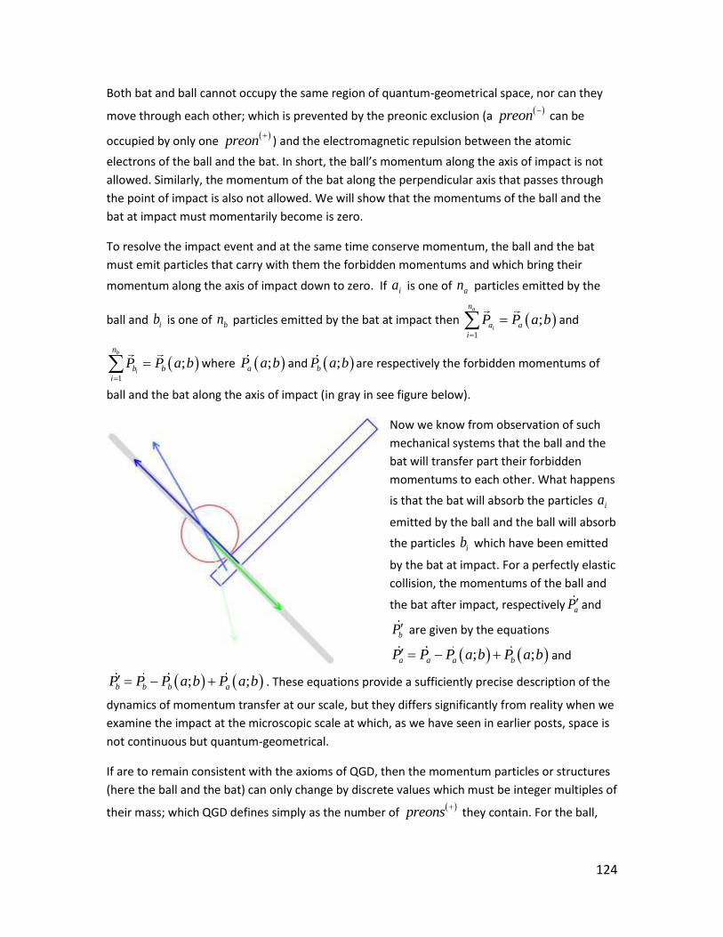
124
Both bat and ball cannot occupy the same region of quantum-geometrical space, nor can they
move through each other; which is prevented by the preonic exclusion (a
preon
can be
occupied by only one
preon
) and the electromagnetic repulsion between the atomic
electrons of the ball and the bat. In short, the ball’s momentum along the axis of impact is not
allowed. Similarly, the momentum of the bat along the perpendicular axis that passes through
the point of impact is also not allowed. We will show that the momentums of the ball and the
bat at impact must momentarily become is zero.
To resolve the impact event and at the same time conserve momentum, the ball and the bat
must emit particles that carry with them the forbidden momentums and which bring their
momentum along the axis of impact down to zero. If ia is one of an particles emitted by the
ball and ib is one of bn particles emitted by the bat at impact then 1
;a
i
n
a a
i
P P a b
and
1
;b
i
n
b b
i
P P a b
where ;aP a b and ;bP a b are respectively the forbidden momentums of
ball and the bat along the axis of impact (in gray in see figure below).
Now we know from observation of such
mechanical systems that the ball and the
bat will transfer part their forbidden
momentums to each other. What happens
is that the bat will absorb the particles ia
emitted by the ball and the ball will absorb
the particles ib which have been emitted
by the bat at impact. For a perfectly elastic
collision, the momentums of the ball and
the bat after impact, respectively aPand
bP are given by the equations
; ;a a a bP P P a b P a b and
; ;b b b aP P P a b P a b . These equations provide a sufficiently precise description of the
dynamics of momentum transfer at our scale, but they differs significantly from reality when we
examine the impact at the microscopic scale at which, as we have seen in earlier posts, space is
not continuous but quantum-geometrical.
If are to remain consistent with the axioms of QGD, then the momentum particles or structures
(here the ball and the bat) can only change by discrete values which must be integer multiples of
their mass; which QGD defines simply as the number of
preons
they contain. For the ball,

125
this means that a aP xm , wherea b
i i
n n
a a a b
i i
m m m m and 1
b
i
n
b
i
a
P
xm
; the quotient
of the Euclidean division of the sum of the momentums of the emitted particles over the mass
of the ball after absorption of the particles so that 1;
b
i
n
b
ia a a a
a
P
P P P a b mm
. This
implies that given the remainder of the above Euclidian division must correspond to sum of the
momentums of the particles emitted by the bat but which the ball is forbidden to absorb. That
is; 1
1 1
b
b b i
i i
n
n n b
ib b a
i i a
P
P P mm
where i is the unique cardinal number attributed to one of bn
particles that are absorbed or one of the bnparticles which absorption by the ball is forbidden
and b b bn n n .
If the impact preserves the physical integrity of the ball, the momentum that is not transferred
to it will be radiated away carried by photons (mostly as infrared). If the impact is such that
physical integrity of the ball is not preserved, then the particles could also be electrons, atoms
or molecules.
Similarly, the bat will absorb photons from the ball and its momentum after impact will be
1
1
a
b i
i
n
n a
ib b b b
i b
P
P P P mm
and 1
1
a
b i
i
n
n a
ib b b b
i b
P
P P P mm
.
Using QGD’s definition of speed we find that the speed of the ball after impact is aa
a
Pv
m
with
1
;
b
i
n
ba i
a
a a
PP a b
vm m
. So if the momentum of the ball along the impact axis is less than
that of the bat, then the ball after impact will have greater momentum, hence speed. If the
momentum of the ball along the impact axis is greater than that of the bat, then the ball will
have less momentum and speed after impact.

126
The physics of baseball bat hitting a baseball illustrates the fundamental mechanisms
responsible for transfer of momentum. It is an example of how the physics at quantum-
geometrical scale determines the behaviour at larger scales. For instance, it can be shown that
much of the same equations we used to describe the physics of baseball can be used to describe
nuclear fission. This is not surprising since, according to QGD, the same forces and laws apply at
all scales.
Newton’s Cradle Everyone is familiar with Newton’s Cradle, a simple mechanism which is thought to demonstrate
the law of conservation of momentum. Paradoxically, the physics of Newton struggles to
describe and explain the behaviour of this simple system of steel balls. In fact, even the full
power of continuous mathematics can only provide an approximation of the behaviour of such a
system and even that must be at the cost of undesirable and awkward complications.
The reader may ask why, today, anyone should bother trying to explain such a trivial device
when there are so many exciting phenomena to which quantum-geometry dynamics can be
applied. Let me ask this question: How can Newton’s cradle be a device demonstrating
Newton’s laws of motion when Newton’s laws of motion cannot explain its behaviour? Also,
since quantum-geometry dynamics claims to explain the dynamics of motion at all scales (and
do so in as a simple and straightforward way), applying it successfully to Newton’s cradle should
be easy. Not to mention, an excellent opportunity to test its validity. It also doesn’t hurt that
building any version of Newton’s cradle is considerably less expensive than, let’s say, a particle
accelerator.
The first thing we must do is equationte the problem in QGD terms. Given a Newton’s cradle
system having n steel balls, when lifting then dropping subset consisting of x numbers of balls,
the impact with set y number of balls will in motion. The problem will be to predict and explain
which balls will be set in motion from the impact as well as determine their momentum and
speed.
We have explained earlier articles that QGD defines the momentum of an object a as
1
am
a i
i
P c
and the its speed as a
a
a
Pv
m where am is its mass in
preons
. Thus
momentum and speed are intrinsic properties independent of the frame of reference.
We also know that the
preons
, the elementary particle that dimensionalizes space to form
quantum-geometrical space, generating an opposing force to changes in momentum so that it
only allows changes in momentum when a aP zm where z N .

127
Conservation of momentum (which is a consequence of the conservation of the fundamental
momentum of
preons
) is such that 1 1
i j
yx
a a
i j
P P
where 1
i
x
a
i
P
and 1
j
y
a
j
P
are
respectively the momentum of a group of x balls pulled and released together and the
momentum of the group of balls set in motion after impact.
Also since ja aP z m where z N , we have
1j
y
a a
j
P yz m
or 1
j
y
a
j
a
P
z my
and
since1 1
i j
yx
a a
i j
P P
then 1i
x
a
ia
P
z my
. That is, the momentum transferred must be an
integer multiple of the mass of a ball. This all we need to explain and predict the behaviour of a
Newton’s cradle system from initial conditions are known. Let’s examine now a few examples
showing how the above applies.
In the example shown in the figure on the left, 3x which leave 2 balls on the right. Now, we
know that the momentum can only be transferred in integer multiples of am , and since the
three balls carry an integer multiple of am (equivalent to an integer number of balls), if it were
to be transferred to the remaining two balls, the resulting change of momentum for each ball
would be a non-integer. Non-integer changes in momentum are forbidden by structure of
quantum-geometrical space.
So the total momentum that can be transferred to the two red balls is 2 aP , 1 aP each, but
since the total momentum of the blue balls is 3 aP that leaves us with 3 2 1a a aP P P .
Since the remaining momentum cannot be transferred, it will be kept by the blue balls. But here
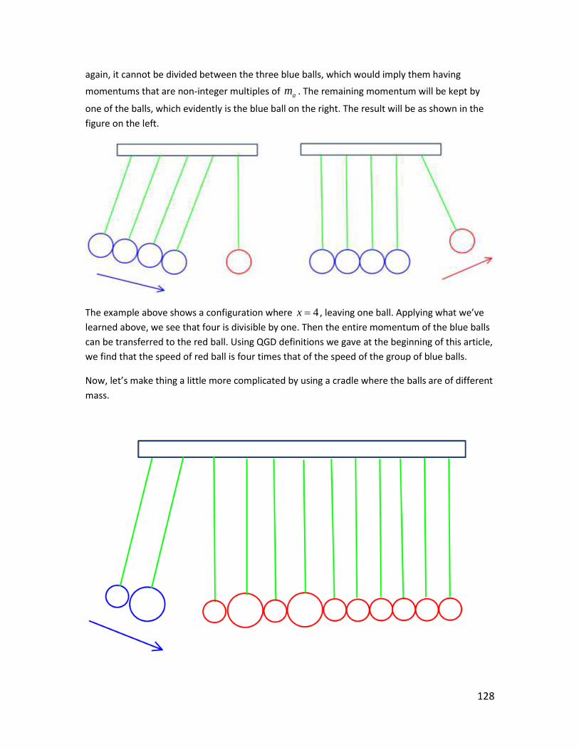
128
again, it cannot be divided between the three blue balls, which would imply them having
momentums that are non-integer multiples of am . The remaining momentum will be kept by
one of the balls, which evidently is the blue ball on the right. The result will be as shown in the
figure on the left.
The example above shows a configuration where 4x , leaving one ball. Applying what we’ve
learned above, we see that four is divisible by one. Then the entire momentum of the blue balls
can be transferred to the red ball. Using QGD definitions we gave at the beginning of this article,
we find that the speed of red ball is four times that of the speed of the group of blue balls.
Now, let’s make thing a little more complicated by using a cradle where the balls are of different
mass.
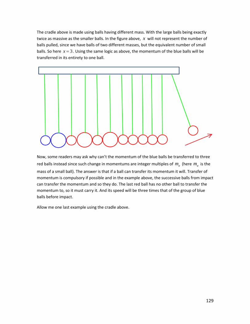
129
The cradle above is made using balls having different mass. With the large balls being exactly
twice as massive as the smaller balls. In the figure above, x will not represent the number of
balls pulled, since we have balls of two different masses, but the equivalent number of small
balls. So here 3x . Using the same logic as above, the momentum of the blue balls will be
transferred in its entirety to one ball.
Now, some readers may ask why can’t the momentum of the blue balls be transferred to three
red balls instead since such change in momentums are integer multiples of am (here am is the
mass of a small ball). The answer is that if a ball can transfer its momentum it will. Transfer of
momentum is compulsory if possible and in the example above, the successive balls from impact
can transfer the momentum and so they do. The last red ball has no other ball to transfer the
momentum to, so it must carry it. And its speed will be three times that of the group of blue
balls before impact.
Allow me one last example using the cradle above.
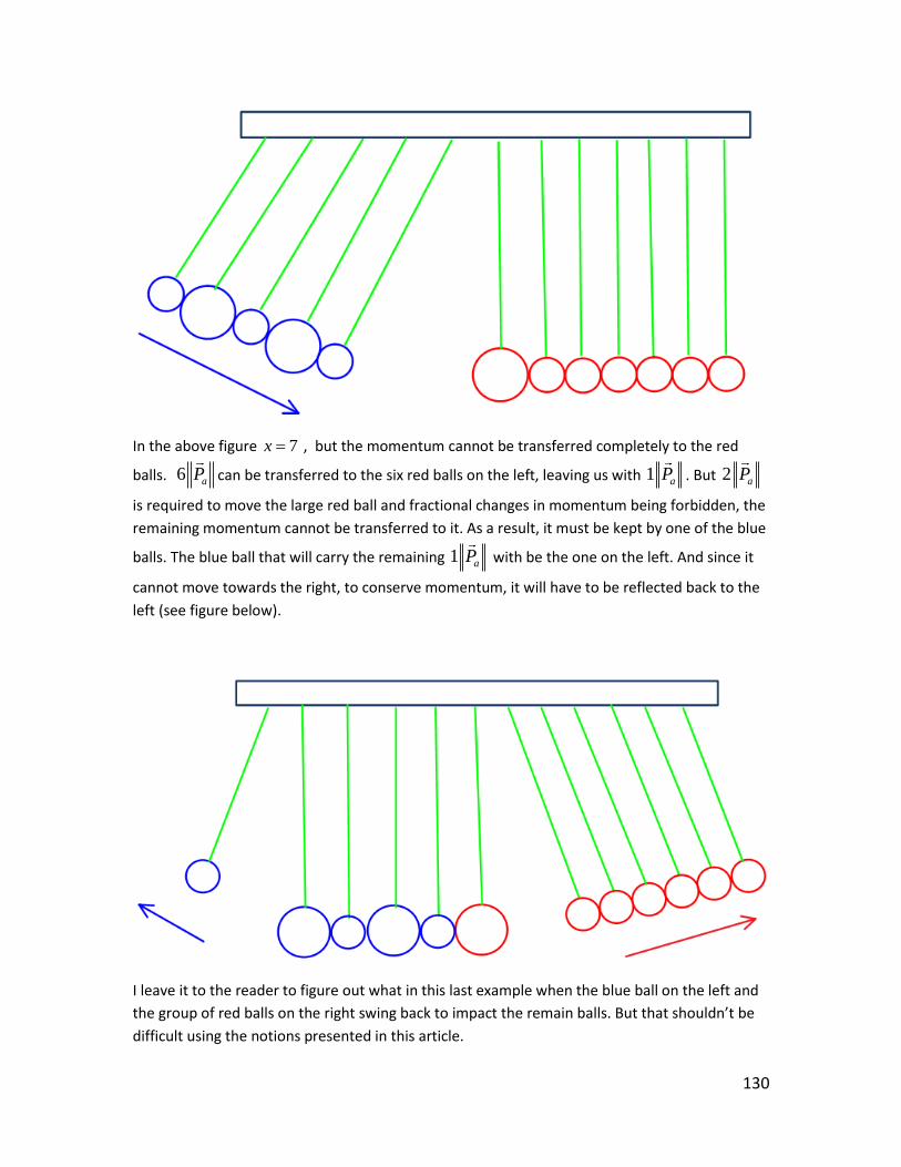
130
In the above figure 7x , but the momentum cannot be transferred completely to the red
balls. 6 aP can be transferred to the six red balls on the left, leaving us with 1 aP . But 2 aP
is required to move the large red ball and fractional changes in momentum being forbidden, the
remaining momentum cannot be transferred to it. As a result, it must be kept by one of the blue
balls. The blue ball that will carry the remaining 1 aP with be the one on the left. And since it
cannot move towards the right, to conserve momentum, it will have to be reflected back to the
left (see figure below).
I leave it to the reader to figure out what in this last example when the blue ball on the left and
the group of red balls on the right swing back to impact the remain balls. But that shouldn’t be
difficult using the notions presented in this article.
131
What we have shown here is that Newton’s cradle can be used to demonstrate at our scale
QGD’s concepts of speed, momentum and conservation of momentum which we have used so
far to describe the motion of particles and structures at the fundamental scale. It follows that
the laws of motion at all scales are consequences of the fundamental scale interactions. As in
the previous article, A Remarkably Simple Proof of the Discreteness of Space, we have shown
that physics at our scale is the observable consequences of physics at the fundamental scale.
Readers may be interested in reading Rocking Newton’s Cradle by S. Hutzler, G. Delaney, D.
Weaire and F. McLeod) as an example of how complicated it can be to describe even this simple
system using classical physics.
States of Gravitationally Interacting Bodies
For a system consisting of n gravitationally interacting bodies,
11
1
;i s ss
n
a i j
j
P a aG
where ia and ja are gravitationally interacting astrophysical bodies of the system,
j i and | 1 | 1 1 | 1 1| 1 1 | 1 | 1
1
; ; ... ;n
i s j s s i s s s i s n s
j
a a G a a G a aG
where
1 | 1 | 1 | 1 | 1 | |; ; ;s i s j s i s j s i s j sG a a G a a G a a and s and 1s are successive states of
the system (a state being understood as the momentum vectors of the bodies of a
system at given co-existing positions of the bodies) and |i s xa is the body ia and its
position when at the state s x . The position itself is denoted |ia s x .
In order to plot the evolution in space of such a system, we must choose one of the
bodies as a reference so that the motions of the others will be calculated relative to it. A
reference distance travelled by our reference body is chosen, refd , which can be as
small as the fundamental unit of distance (the leap between two preons
or preonic
leap) but minimally small enough as to accurately follow the changes in the momentum
vectors resulting from changes in position and gravitational interactions between the
bodies.
So given an initial state s , the state 1s corresponds to the state described by the
positions and momentum vectors of the bodies of the system after the reference body
travels a distance of refd . For simplicity, we will assign 1a to the reference body.

132
1| 1 1| 1
| 1 |
1| | 1 | 11
| | 1 | 11
; |
1 ... | ...
; |
s s
n s n s n
n
a a s j s a sj
n
a a n s j s a sj
P P G a a
s
P P G a a
(5)
Using the state matrix, the evolution of a system from one state to the next is obtained
by simultaneously calculating the change in the momentum vectors from the variation
in the gravitational interaction between bodies resulting from their change in position.
Changes in the momentum vectors have are as explained earlier. Changes in position
are given by 1
| 1 |i
i i i
i
a ref
a s a s a
a a
v dP
v P . The distance travelled by ia from s to 1s is
1
ia
ref
a
vd
v (for 1j , the distance becomes simply refd ) and distance between two bodies
of the system at state s x is ; | | |i j i ja a s x a s x a s xd . It is interesting to note here that
that for i j , then ; | 0
i ja a s xd , so that
1 | 1 | 1 | 1 | 1 | |
2 2; | 1 ; | 1 ; | ; |
; ; ;
2 2
0
i i i j i i i i
s i s j s i s i s i s i s
a a s a a s a a s a a s
a a a a
a a a a
G a a G a a G a a
d d d dm m k m m k
m m k m m k
,
the variation in the gravitational interaction between a body with itself is equal to zero,
which implies that its momentum vector will remain unchanged unless 1n and
| | 11
; 0n
n s j sjG a a
. This is the QGD explanation of the first law of motion.
133
Introduction to QGD Cosmology Most theories of the genesis and evolution of the Universe invoke one or more
extraordinary and spontaneous events, triggered by some extraordinary mechanism
which operates under extraordinary but now inexistent conditions. Simply put, they
speculate rather than deduce or infer.
The Big Bang Theory for instance, the dominant cosmological theory, speculates that the
entire Universe was concentrated in one single point, a singularity, which expanded into
the present state of the Universe.
The Standard Model speculates that at some point, its hypothetical Higgs field was
somehow turned on and caused the slowing down of fundamental particles (which until
then only travelled at the speed of light) forcing them to acquire mass and form matter.
Both the above theories imply the continuity of space and the belief that time is
physical, that is, they imply the existence of space-time.
In the case of the Standard Model, the use of continuous functions leads to a gradual
increase in the degree of complexity of the model which continuously adds conceptual
patches in an attempt to reconcile it with observations. The Standard Model apparently
works when applied to a very restricted domain of physical reality, but collapses
completely when it tries to apply its principles to other scales of reality. The most
spectacular demonstration of the Standard Model’s unreliability is its prediction of the
vacuum energy density which disagrees with observations by 107 orders of magnitude.
This prediction is considered the worst theoretical prediction in the history of physics.
QGD cosmology makes no attempt to introduce extraordinary mechanisms or
conditions. QGD does not speculate from hypothetical past mechanisms or conditions
which do not exist in the present phase of the Universe. Rather QGD considers
fundamental laws to be invariable. That the laws governing the evolution of the
Universe were, are and will always remain the same, so all the different phases of the
evolution of the Universe can be deduced from an understanding the present conditions
and physical laws.
Quantum-geometry dynamics Cosmology is based on QGD’s fundamental principles and
the QGD Law of Conservation.
But before we proceed to equationte these laws, we need to draw clear and
quantifiable definitions of what constitutes the Universe. QGD proposes the following:
134
1. The Universe is the sum of all preons
and
preons
, which implicitly includes
their interactions, structures and properties.
2. The size of the Universe is equal to the space dimensionalized by preons
. It is
the tri-dimensional amplitude of the n-gravity field.
3. The mass of the Universe is equal to the total number of preons
and its
energy is the product of the number of preons
it contains by the
preon
energy or
U UE m c .
The Material and Spatial Dimensions of the Universe When we think of the Universe, we think of what we observe through telescopes. We think of
planets, stars, galaxies, galaxy clusters; the material structures of the Universe. When we study
the Universe, we do so by observing the light or particles emitted by material structures, but not
the entire Universe is observable. We can only observe what is made of matter because only
matter can interact with the instruments we use for observation. Yet the Universe is made of
more than matter; it is also made of space. And if QGD is correct, then space is made from
preons
which implies that space is quantum-geometrical.
Virtually all of physics considers space to be an amorphous expanse in which physical systems
exist and interact. As a consequence all physics theories are theories of matter (or matter and
energy to be precise). Quantum-geometry dynamics too is a theory of matter, but it is also a
theory of space. Also, according to QGD, not only is space quantum-geometrical and emergent,
it also determines the very structure of all matter.
Principles of QGD Cosmology
First Principle of QGD Cosmology or Principle of Conservation of Physical Properties:
Whatever laws and mechanisms that exist today existed at the beginning of the Universe
whatever laws and mechanisms that existed at the beginning of the Universe must exist
today and will always exist.
The laws and mechanism that govern the Universe and its evolution are unchanging,
absolute and universal.
In other words: QGD proposes that there never were any special conditions, events or
mechanisms that only existed in the primordial universe which produced the matter in
the universe only to disappear right after.
135
From QGD’s First Principle of Cosmology, it follows that in order to gain some
understanding of how the Universe evolved all one needs to understand the
fundamental laws of physics, its mechanisms and the conditions that prevail now.
The fundamental laws of physics are those which govern the two fundamental particles
and their associated forces. The mechanism by which matter forms are axiomatically
derived from the fundamental properties of preons
and
preons
. Also derived from
the fundamental properties is how particles and physical structures interact to produce
the gravity effect and the electromagnetic effects and all forces and yet to be discovered
known.
Principle of Strict Causality:
Given any two types of physical objects where the objects of the first type are
constituents of the objects of the second type, then the pre-existence of the objects of
the first type is an essential and necessary condition to the formation of the objects of
the second type.
The principle of strict causality being based on properties of physical reality, it offers the
possibility of understanding the evolution of the Universe as sequences of events that
are causally connected. The principle of strict causality effectively replaces the relational
concept of time.
The principle of strict causality implies is that the Universe does not evolve with time,
but changes from state to state as a consequence of concurrent series of events causally
related.
The reader will notice that the Principle of Causality is non-relativistic and neither calls
upon the concept of time nor the concept of observer. It only takes into account the
quantum-geometric structures of the physical objects and their movement within
quantum-geometric space.
Law of Conservation:
Conservation of Space
QGD proposes that it be the repulsive force of n-gravity acting between
preons
that
generates space (n-gravity being the fundamental force intrinsic to
preons
). Since
preons
are fundamental particles, they obey the law of conservation which states that nothing
fundamental can be created or destroyed. It follows that there must be a finite number of
preons
, which in turn implies that there is a finite number of interactions, thus a finite
136
amount of quantum-geometrical space. Therefore, as large as it appears to be, space must be
finite.
Particle Formation and Strict Causality
QGD follows the principle of strict causality, which is short for saying that the formation of any
non-fundamental physical object requires the pre-existence of its constituents and the pre-
existence of a state that is directly and causally linked to it. Fundamental objects, being
fundamental, pre-exist everything else (post-exist everything else as well).
The strict causality implies that any structure requires the pre-existence of its components may
appear trivial, but it is a principle that some theories feel is fine to violate. Other theories, such
as string theory, can’t tell which particles may be components of which other particles (see
Leonard Susskind’s lectures of reductionism here). As a result, theories that violate strict
causality may ambiguously indicate that reality can get more complex the closer we approach
the fundamental scale.
There is no such ambiguity in quantum-geometry dynamics. Strict causality implies that reality
get simpler the closer we get the fundamental scale. At which scale QGD predicts the existence
of only two fundamental particles and two fundamental forces. Reality can’t get any simpler.
QGD shows that all laws of physics can be derived from a simple of set of axioms which is
complete and consistent.
This, of course, contradicts physical interpretations of Gödel’s incompleteness theorem. But if
the Universe is made of a finite set of fundamental particles which combine in accordance to a
finite set of fundamental laws to produce physical reality, then it follows that Gödel's first
incompleteness theorem is, at least in its present form, wrong. Also, if you believe that the
fundamental components and laws are a consistent and that the Universe is a coherent system,
then Gödel's second incompleteness theorem must also be wrong.
It follows the Universe is found to be complete and consistent system, then Gödel must be
revised and Hilbert's program must be reinstated.
If the universe is found to be both consistent and complete, that is, fundamental particles and
the laws that govern them are consistent and all that results from them remains part of the
Universe (completeness), then all physical processes are emergent from a finite axiomatic set of
fundamental particles (implied by the law of conservation) and their intrinsic properties. Now,
that means that not only are the basic physical interactions emergent, but all processes,
including environmental, social, cultural and neurological processes emerge from the
fundamental axiomatic set.
QGD argues that, as abstract mathematics may be from reality, they are the result of mental
processes, which are necessarily physical so that they, themselves, can be derived from the
fundamental laws of physics. In that context, it doesn't matter what the construct is (a painting,
137
a film, a poem or a mathematical theory), it must be emergent and can theoretically be derived
from the fundamental axiomatic set.
The Cosmic Microwave Background Radiation
Quantum-geometry dynamics describes the initial state of the Universe as being one in which
preons
were free and distributed uniformly throughout the quantum-geometrical space.
Following this initial state, low mass photons started to form in accordance to the mechanism
we have described earlier. When the photons produced were of sufficient mass (which
corresponds to the radio frequency in the wave model of light) , they formed what we call the
microwave cosmic background radiation; the isotropy of the CMBR being easily explained by the
isotropy of the
preon
distribution if the Universe. The
preon
density being greater than it
is now, the rate of production of photons produced was much greater.
Most
preons
are still free today and still form photons (though at slightly the lower rate)
which add to the CMBR.
Cosmic Neutrino Background
Following the mechanism of formation of particles and the isotropy of the distributions of
preons
, the universe must contain low mass neutrinos which, because of the analogy to the
CMBR, we can call the cosmic neutrino background. But unlike the CMBR, which photons are
sufficiently massive to interact with instruments, the CNB neutrinos interact too weakly to be
detected directly.
Small Structure Formation
The strict causality principle, which requires the pre-existence of a structure’s components,
implies that photons and neutrinos formed electrons, positrons and neutrinos. In fact, the well-
known electron-positron annihilation is simply the reverse of the mechanism of particle
formation.
Large Structures
The formation of large structures also follows the principle of strict causality. It implies the
formation of larger particles, then nuclides (the components of the atomic nucleus) then light
atoms. These eventually formed planets, stars and galaxies. The formation of increasingly
massive structures (elements) continued in stars where the gravitational interactions are
sufficient for the formation of elements.
Black Holes and Black Holes Physics QGD predicts the existence of structures which exerts such gravitational pull that photons
cannot escape. But contrary to the classical black holes predicted by relativity, the black holes
predicted by quantum-geometry dynamics are not singularities. The QGD exclusion principle
which states that a
preon
cannot be occupied by more than one
preon
implies that
quantum-geometrical space imposes a limit to the density any structure can have. The density
138
of black holes is also limited by the fact that
preons
, being strictly kinetic, they must have
enough space to keep in motion. It follows that black must have very large yet finite densities.
Angle between the Rotation Axis and the Magnetic Axis
The effect of the helical motions of the electrons in direction of the rotation of a body adds up
so that, at a large scale, the body behaves as a single large electron which though helical
trajectory around the body interacts with the neighbouring preonic region to generated a
magnetic field.
Since the magnetic field is the result of the polarization of free
preons
along the loops of the
helical trajectory, and since the inclination of these loops increases with the speed of rotation,
so does the angle between these loops and the axis of rotation inscreases. It follows that the
angle between the axis of rotation and the magnetic axis for bodies of given material
composition is proportional to the speed of rotation about its axis and its diameter.
This angle between the axis of rotation and the magnetic axis is small for slowly rotating bodies
but can never be so small that the axes coincide. From the above, it also follows that a faster
rotation not only implies a larger the angle between the rotation axis and the magnetic axis is,
but also a flattening of the magnetic field and an increase in its intensity.
The Inner Structure of Black Holes
To understand the structure of a black hole we will look at what happens to a photon when it is
captured by it the gravitational pull.
The model for light refraction that we introduced in earlier articles can be applied directly to
photon moving through a black hole. Since we assume that the black hole is extremely massive,
its trajectory will bring it towards the center of the black hole.
When moving along the magnetic axis of the black hole, the component
preons
of the
preon
pairs of the photon are pulled away from each other, splitting the photon into free
preons
which may or not recombine into neutrinos. This works as follow:
As we have seen earlier in this book, the force binding the
preons
of a
preon
pairs is
gravitational. The QGD gravitational interaction between particles at the fundamental scale is
2
2; a b
d dG a b m m k
, and since a and b are
preons
, 1a bm m and since
1d , the binding force between two
preons
of a
preon
pair is equal to 1k .
For a photon moving along the magnetic axis, we have and 1 2 1 1; ; 1G p R G p R k
where 1p
and 2p
are the component
preons
of a
preon
pair of a photon.

139
The regions 1R and 2R , on each side of the black hole axis are equally massive regions. If we
call 1Rand 2R the regions each side of 1p
when the photon’s trajectory is aligned with the
black hole axis then 2 1R R and 1 2 1 1; ; 1G p R G p R k
. Similarly, if we call 1R and
2R the region on the each side 2p
then 1 2R R and 2 1 2 2; ; 1G p R G p R k
. So
the force pulling the
preons
of
preon
pairs being greater than the force that binds them,
the
preon
pairs are split into single
preons
.
How do we that the gravitational forces within a black hole are sufficiently strong to cause the
photons to be broken down into
preons
? If the gravitational forces within the black hole
were not enough to breakdown the photons, then photons moving along a black hole axis would
escape into space making the black hole visible. Since black holes do not emit light, then the
gravitational interactions must be strong enough to break photons down into
preons
and
neutrinos.
The image above shows how a simple two
preons
photon is split into two free
preons
which because of the the electro-gravitational interactions move back toward the magnetic axis.
But, because the quantum-geometrical space occupied by the black holes is densely populated
by particles which affect randomly the trajectories of the single
preons
, our two
preons
arrive at the magnetic axis of the black hole at different positions. And if they are in close
enough proximity, the single
preons
will combine to form a neutrino which structure, not
being made of
preons
pairs, remains structurally unaffected by the intense gravitational
interactions within the black hole.
Once the trajectories of the
preons
or the neutrino coincides with the magnetic axis of the
black hole, the
preons
or neutrinos will move through the center of the black hole and will
140
exit it. Preons
and neutrinos can escape the gravitation of the black hole because
gravitational interactions, though it affects the directions of
preons
, doesn’t change their
momentums which, as we have seen in earlier articles is fundamental and intrinsic (the
momentum of a
preon
is c where c is momentum vector of a
preon
).
It follows, that all matter that falls into a black hole will be similarly disintegrated into
preons
and neutrinos, which will exit the black hole. The black hole will thus radiate
preons
and
neutrinos, in jets at both poles of their magnetic axis of rotation. Since
preons
and neutrinos
interact too weakly with instruments to be detected by our instruments, they are invisible to
them. In order to see the
preons
-neutrinos jets from a black hole, instruments may need
detectors larger than our solar system. However, the jets can be observed indirectly when they
interact with large amount of matter when the polarized
preons
and neutrinos they contain
impart it with their intrinsic momentum. It is worth noting that polarized preons and neutrinos
jets, as described by QGD, would contribute to the observed dark energy effect.
Based on QGD’s model of the black hole, we can predict that the
preons
/neutrino jets will
form an extremely intense polarized
preons
field along the magnetic axis creating the
equivalent of a repulsive electromagnetic effect at both poles. The polarized preonic field would
repulse all matter on their path, which may explain the shape of galaxies.
From what we have discussed in the preceding section, we can define a black hole as an object
which mass is such that it can breakdown all matter, including photons, into
preons
.
The QGD model of the physics of black hole has another important implication. The
preons
and neutrinos resulting from the breakdown of a particle or structure are indistinguishable from
the
preons
or neutrinos resulting from the breakdown of any other particle or structure. This
means, if QGD is correct, that all information about the original particle or structure is lost
forever. That said, since this consistent from QGD’s axioms set and since, unlike quantum
mechanics, QGD does not require that information be preserved, the loss of information it
predicts does not lead to a paradox ( see this article for an excellent introduction to subject).
Neutron Stars, Pulsars and Other Supermassive Structures
When the mass of a structure is sufficient to bind photons, but insufficient to breakdown
photons, electrons and positron, we get a stellar structure which can emit these particles.
The internal gravitational interactions will redirect particles towards the magnetic axis of the
stellar structures where, when its trajectory coincides with an axis, the gravitational force from
the stellar object acting on the particles will cancel out and the particle will escape the object
into outer space. Such structures may correspond to what we call neutron stars. So what
141
distinguishes neutron stars from black holes is that we have 1 2 1 1; ; 1G p R G p R k
and 2 1 2 2; ; 1G p R G p R k
. That is, the gravitational force within the neutron star
which acts on particles is insufficient to breakdown photon, electron and positrons.
Another prediction is that distinguishes quantum-geometry dynamics is that neutron stars are
not composed of neutrons. The internal gravitational forces being such that they would break
down all particles into neutrinos, photons, electrons and positrons.
Pulsars
When a neutron star rotates at a sufficiently high rate, it interacts with the preonic field in such
a way that it creates an intense magnetic field. Such magnetic field will be sufficiently strong to
curve the trajectory of all neutrinos, photons, electrons and positrons that move past its surface
back into pulsar. Particles that move along its axis of rotation, along which the electromagnetic
force cancel out, will escape at the magnetc poles producing the known bidirectional emission
characteristic of pulsars.
Cosmological Consequences
The mechanism of emission of
preons
and neutrinos will be continue until the black hole has
been completely evaporated; which it will after it has absorbed all matter in its vicinity. By this
mechanism,
preons
which had formed particles and structures are disintegrated into free
preons
and neutrinos which are then returned to the universe.
In later phases, the free
preons
and neutrinos will form new particles and structures,
eventually leading to the formation cosmic structures and black holes. And later, due to
gravitational interactions, these cosmic structures will ultimately be absorbed by black holes,
which break down matter into
preons
and neutrinos, repeating the cycle indefinitely.
Locally Condensing Universe This is one the most distinctive aspect of the QGD cosmology. If follows from the axioms of QGD
that the size of the Universe, defined as the space emerging from the interactions between
preons
is constant, but within that space massive structures will gradually collapse towards
their center.
To the observer, a locally condensing universe is nearly indistinguishable from an expanding
universe. For instance, the distance between galaxies progressively increases in both locally
condensing universe (LCU) and expanding universe (EU). And in both the rates at which the
galaxies retract from each other increases, which indicates that galaxies retract at accelerated
rate in both the LCU and EU. So if both LCU and EU are nearly indistinguishable to the observer,
how do we know which is correct? Is there any evidence which would support LCU?
142
The observational evidence exists and has been known from some time as redshift anomalies.
The redshift is simply the shift of the frequency of light coming from a moving source (which is
understood to be analogous to the Doppler Effect for sound). Established theories belief that
the faster the relative speed of the source of light away from the Earth, the greater the redshift
of the light coming from that source. The magnitude of the redshift is used to calculate the
distance between galaxies and the rate at which they recede from each other.
QGD implies that the redshift effect is dependent on the speed of the emitter but independent
from the speed of the observer. This will be discussed in the section titled Mapping the
Universe.
According to the Big Bang theory, which is the dominant theory of the expanding universe, the
further away galaxies are, the faster they will recede from us. This implies that neighboring
cosmic structures (galaxies, quasars, etc.) would recede from us at the same rate, thus have the
same redshift. This is generally true, but there are an increasing number of observations that
show neighboring cosmic structures having significant differences in their redshifts. This would
indicate that the rate at which they recede from us differs by many orders of magnitude.
Redshift anomalies (and there are now thousands of them) are in direct opposition with the Big
Bang and other expanding universe theories.
Yet, redshift anomalies support the idea of a locally condensing universe. Not only do redshift
anomalies support QGD cosmology, they are predicted by QCD cosmology. Redshifts, according
to QGD, are not an indication of the rate at which they galaxies recede, but the rate at which
they collapse (which itself is a function of the density of the galaxy or cosmic structure). The
acceleration of the rate at which galaxies recede is also consistent with rate at which they would
collapse under the gravitational effect described by QGD.
The rate of collapse of cosmic structures follows the same laws of motion that have been
described in earlier chapters. As such it is affected by their mass and density, but also by the
gravitational interactions between them. Using the QGD gravitational interaction equation, the
rate of collapse between galaxies will be affected by dark energy or dark matter effects
depending on the distance between them. The dark energy and dark matter effect will also
determine the shapes of the interacting galaxies. Given certain distance exceeding a certain a
value, n-gravity will be dominant (the dark energy effect) resulting in a flattening of the galaxies
along the axis that connects them. While at distances lower than the equilibrium point, p-gravity
becomes dominant (the dark matter effect) and the shape galaxies will expand along the axis
connecting them.
The same principle explains why the material universe (that part of the universe where matter is
concentrated) is nearly flat (something that the Big Bang and other expanding universe theories
can’t explain). Thus the universe should become flatter as it evolves.

143
Consequences for Particle Physics
Particle accelerators, such as CERN’s large hadron collider, are extraordinary tools that attempt
to recreate on a microscopic scale the conditions that prevailed at the beginning of the
Universe. The hope is that by recreating the conditions immediately following the Big Bang will
reveal the fundamental particles and states that existed at the very beginning of the Universe.
This is a valid approach if the Big Bang theory’s assumption that the Universe evolved from a
singularity is correct. But what if, as QGD suggest, the Universe evolved from an isotropic state?
If such is the case, then the conditions recreated in particle colliders are not those that prevailed
at the beginning of the Universe, but conditions QGD predicts appeared at later stages of the
evolution of the universe. That is; conditions characterized by dense preonic structures such as
those existing massive cosmic objects. Thus, particles colliders do not reveal fundamental
reality, but an emergent reality. In other words, trying to discover fundamental reality using
particle accelerator is like looking at the wrong end of microscope to reveal the microcosm or at
the wrong end of a telescope to observe the macrocosm. What any instrument reveals to us
depends on the theory we use to interpret what it is showing us.
That is not to say that such instruments as the LHC are useless. On the contrary, such
instruments are essential to our understanding of reality. It’s only that what they show us is not
fundamental reality, but processes that came into existence at states that followed the initial
isotropic state of the Universe.

144
The Preonic Universe
According to the principle of strict causality we can deduce the following:
Preons
and preons
, are fundamental. As such and in accordance with the
fundamentality theorem, they have no components; hence they require no pre-existing
conditions to exist. From this and to be in accordance with the Law of Conservation, all
preons
and preons
always existed.
That is, preons
and
preons
not only existed at the origin of the Universe. They are
the origin of the Universe.
It follows that in its initial phase, the Universe consisted of preons
uniformly
distributed throughout the entire quantum-geometric space of the Universe; the
preonic universe.
The theory proposes that the n-gravity and p-gravity fields were in perfect equilibrium.
That is
2 2( ) / 2 ( ) /2U U U Uk m m Vol Vol
Where Um is the mass of the preonic universe and UVol is the number of preons
its
space is composed of. But since 2
lim 0x
x
x
, at the macroscopic scale, the relative
value of Um and UVol become negligible and we can simply write10:
2 2/ 2 / 2U Ukm Vol
Also, from the QGD definitions of heat, temperature and entropy we know that, since in
the primordial universe contained only free preons
, the heat it contained was equal
to its energy, that is 1
Um
i U
i
Heat c m c
, its temperature was U
U
m c
Vol and its entropy
being the difference between its energy and heat, and heat and energy being equal in
the preonic universe, its entropy was equal to zero.
10
Since QGD implies that all quantities are finite, even mathematical quantities, represents the largest theoretical quantity of any physical property. In this equation it may be taken as the number of n-gravity interactions in the universe.

145
Interestingly, since 2
U UVol km the temperature of the preonic universe is given by
2
U
U
m c c
kkm .
Hence, the temperature of the preonic universe is a ratio of c and k ; the two
fundamental constants of quantum-geometry dynamics.
146
Mapping the Universe
Emission Spectrum of Atoms
Everything we know about the universe we learned from photons. We detect cosmic photons
with senses and instruments and from their physical properties we estimate the size, speed,
direction, position and composition of each of their sources. In short, cosmic photons allow us
to map out the Universe. The maps we now use have been drawn from interpretations of the
signals we receive. And these interpretations are based on theories which are founded on the
wave model of light.
The main tool used to determine position, direction and speed of a stellar object is provided by
what is called the redshift effect. The redshift effect is simply the change in frequency of light
attributed to the Doppler effect and is expected to occur when the emitting source is speeding
away from us. The magnitude of redshift is understood to be proportional to speed of the
source and is be used to calculate its distance from us. Maps of the observable universe are
made by compiling data received from all observable sources. The problem, if QGD is correct, is
that those maps are built on the assumption that light behaves like a wave and that,
consequently, the Doppler effect applies. But if, as QGD suggests, light is singularly corpuscular,
will a map based on QGD’s interpretation of the redshift and blueshift effects agree with the
maps based on the wave model of light? Before answering the question we will first discuss how
QGD explains the redshift effect.
We have shown that quantum-geometrical space itself exerts a force on an object and that any
change in momentum of an object must be an integer multiple of the mass of the object (see
Reflection and the Photoelectric Effect). That is, for an object a of mass am , a aP xm
where x N . This applies to the components of an atom that are bombarded by photons. For
instance, if a is an electron bombarded by a photon b having mass bm , which momentum we
have learned is equal to bm c , then a will absorb b only if b am c xm . Similarly, the allowable
changes in momentum a aP xm must also apply to the emission of photons by an electron.
The allowable changes in momentum determine the emission spectrum of the electrons of an
atom.

147
In the figure above, we have the visible part of the hydrogen emission spectrum. Here the first
visible band correspond to a change in momentum of the electron a by emission of a photon
with momentum ib am c im . Notice that the lowest possible value, which is at the far end of
the spectrum is given when 1i . Each emission line corresponds to allowable emission of a
photon from an hydrogen atom’s single electron. In agreement with the laws of motion
introduced earlier, each emitted photon has a specific momentum ibm c (hence, a specific mass
ibm ). For values of x i and 3x i which are respectively towards the infrared and
ultraviolet; the momentum puts them outside the boundaries of visible light.
For an atom a having n components electrons ia in its outer orbits (the ones that will interact
most with external photons) where 1 i n and having mass iam the emission lines of its
component electrons ia corresponds to photons ib such that ib i am c x m and its spectrogram
is the superposition of the emission lines of all its electrons. An example of the superimposition
of the emission spectrums of the electrons of iron is shown in the illustration below. Note that
an electron can have only one change in momentum at the time, emitting or absorbing a photon
of corresponding momentum. So emission spectrograms are really composite images made
from the emission of a large enough number of atoms to display the full emission spectrum of
an element.

148
QGD’s Interpretation of the Redshift and Blueshift Effects
Now that we have described and explained the emission spectrum of atoms we can deduce the
cause the redshifts and blueshifts in the emission lines of the emission spectrum an atom. We
saw earlier that the emission of a photon by and electron a corresponds to a change in the
electron’s momentum such that a aP xm where x N . So a redshift of the emission
spectrum of an element implies that photons emitted by its electrons ia are less massive than
photons emitted by the electrons ia of a reference atom of the same element (most often, the
reference atom is on Earth). This means that i ia axm xm sot that
i ia am m . That is, the mass
of electron ia belonging to an atom of an element from a distance source is smaller than the
mass of the corresponding electron ia belonging to the atom of the same element on Earth. In
the same way, the blueshift of the emission lines of the emission spectrum of an atom implies
that i ia am m .
So, according to QGD, the redshift and blueshift effects imply that the electrons of the light
emitting source are respectively less and more massive than the local reference electron a .
Therefore, quantum-geometry dynamics does not attribute the redshifts and blueshifts effects
to a Doppler-like effect (which in the absence of a medium doesn’t make sense anyway) and, as
a consequence, these effects are not speed dependant. Hence redshifts and blueshifts provide
no indication of the speed or distance of their source.
From the mechanisms of particle formation introduced earlier, we understand that though all
electrons share the same basic structure they can have different masses. As matter aggregates
though gravitational interactions, electrons absorb neutrinos, photons or
preons
and
gradually become more massive. It follows that redshifted photons must be emitted by sources
at a stage of their evolution that precedes the stage of evolution of our reference source.
Similarly, blueshifted photons being more massive were emitted at a stage of their evolution
that succeeds that stage of evolution of our reference source. However, it can’t be assumed that
sources of similarly redshifted photons are at similar distances from us unless they are part of a
system within which they have simultaneously formed. The sources of similarly redshitted
photons may be at greatly varying distances from us. Also, a source of blueshifted photons can
be at the same distance as a source of redshifted photons would be. Therefore, there are
important discrepancies between a map using QGD’s interpretation of the redshift and blueshift
effects and one that is based on the classical wave interpretation of the same effects.
So though they provide no information about to the distance of their source (much less about
their speed), redshifted or blueshifted photons inform us of the stage of evolution of their
sources at the time they were emitted. Also, since sources of similarly redshifted (or similarly
blueshifted) photons have similar mass, structure and luminosity, it is possible to establish the
149
distance of one source of redshifted photons relative to a reference source of similarly
redshifted photons by comparing the intensity of the light we receive from them.
Gravitational Telescopy
As we have seen, although we can indirectly estimate the distance of source of photons relative
to another, there is no direct correlation between distance, direction or speed of a stellar object
and how much the photons they emit are redshifted or blueshifted. However, according to QGD,
it is theoretically possible to map the universe with great accurately by measuring the
magnitude and direction gravitational interactions using a gravitational telescopy. And, unlike
telescopes and radio-telescopes, gravitational telescope are not limited to the observation of
photon emitting objects.
More importantly, if QGD’s prediction that gravity is instantaneous, then a map based on the
observations of gravitational telescopes would represent all observed objects as they currently
are and not as they were when they emitted the photons we receive from them.
Mass Change of Photons over Distance
After the photons leave their source and if they are not absorbed by larger structures, they may
interact with
preons
, neutrinos or other photons, combining with them to form photons
having higher mass (and energy). Hence, most photons coming from distant source will
“blueshifted” relative to their source. And the greater the distance the photons travel the more
likely will their mass. It is therefore possible that photons which were originally redshifted, if
they travel a long distance enough, become blueshifted by the time they reach us. That said,
because most interactions will be asymmetrical, photons which acquire mass by absorption of
other particles will most likely be scattered and will contribute to the cosmic background
radiation. Some of these photons which acquire enough mass may correspond to what is known
as fast radio bursts.
Cosmological Implications
The notion that the universe is expanding is based on the classic interpretation of the redshift
and blueshift effects, but if QGD is correct and redshift and blueshift effects are consequences
of the stage of evolution of their source, then the expanding universe model loses its most
important argument. The data then becomes consistent with the locally condensing universe
proposed by quantum-geometry dynamics.

150
Application to Unsolved Problems All physics theory must be consistent with reality. Not only must it explain real world
phenomena, it must make verifiable predictions. That is, it must be falsifiable.
Though we have used QGD to make some original and verifiable predictions for we a
number of phenomena, the theory, if it is correct, must also offer solutions (or at least
propose directions that will lead to possible solutions) to as-of-yet unsolved problems in
physics.
In the first edition of this book I had included a lists of such problems and provided new
interpretations based on QGD and offered some solutions. For this edition I thought
better to let you, the reader, reinterpret those problems yourself using the knowledge
acquired from these pages and find your own solutions.
Those interested in the exercise will find a list of some of the most important unresolved
problems in physics here. Hope you will enjoy the challenge.

151
Addendum: Principles, Axioms and Theorems of QGD This section resumes the core ideas introduced in this book.
Principle of Strict Causality
Quantum-geometry dynamics admits no spontaneous phenomenon. A photon, for
example, can never spontaneously transform into a particle even when, as the Standard
Model proposes, the amount of energy it carries is equivalent to that of the particle or
particles it would transmute into. The “spontaneous” transformation of a photon into a
particle will then be the result of a deterministic mechanism.
All phenomena that implies changes in direction and structure are caused by events;
that is, the interaction between particles, higher structures or combinations of them.
This will be explained in detail in following chapters.
Conservation Law and the Fundamentality Theorem What is considered fundamental has often changed over the course of History so what we now
consider fundamental may reveal itself to be non-fundamental by our successors. How we
define "fundamental" has profound consequences on the way we interpret reality or create
models. QGD uses the following definition of what is fundamental:
An aspect of reality is fundamental if it is absolutely invariant
Axioms and Theorems of Quantum-Geometry Dynamics
As mentioned above, rather than using the deconstructive approach which consists of
gathering observational and experimental data and mathematically processing it in an
attempt to extract or deduce from it the fundamental laws of the Universe, QGD favours
a constructive approach which consists of deducing the theory from a finite set of
axioms.
This approach results in a consistent, complete theory which is applicable to explain
and/or predicts the outcome of interactions at all scales of reality. And because the
theory is developed from a single set of axioms, it is internally consistent and precludes
competing and often contradictory theories.
Below is a summary of the axioms and corollaries from which quantum-geometry
dynamics is constructed. These will be fully explained in detail the following chapters.
There are only two fundamental particles: the preon
and the
preon
.
152
This implies all other particles, even those which are now considered elementary, are
composite.
This means that the distance between two preons
is created by n-gravity field
between them. And 𝑔− represents the unit n-gravity force acting between two
preons
.
There are only two fundamental forces, each associated to one of the fundamental
particle. One is an attractive force, which we will call p-gravity, and the other, a
repulsive force, which we will call n-gravity.
What this implies is that all other forces, known and unknown, are effects resulting from
p-gravity and n-gravity.
Space is discrete.
This is probably the most impactful axiom of quantum-geometry dynamics. What it
means is that space cannot be infinitely subdivided in smaller and smaller parts. This
implies a limit beyond which space can no longer be subdivided. According to QGD,
there is a smallest possible distance.
Space emerges from the interactions between preons
.
Space is finite
If space is generated by intrinsic force acting between fundamental particles, then, by
definition, these particles must obey the law of conservation. That is, there must be a
finite number of such particles. And as a consequence, space must also be finite.
preon
are the fundamental particle of mass.
While preons
generate space by repelling each,
preons
on the other hand are
kinetic. In fact, preons
are the fundamental kinetic particles. They are defined by
their continuous movement and do not exist at rest. Preons
move by leaping from
preon
to the next preon
which implies that the
preon
leap is the fundamental
unit of movement.
153
Also, that preons
are in continuous movement implies that there needs to be more
preons
in the Universe than there are
preons
.
The magnitudes of n-gravity and p-gravity in the Universe as a whole are equal.
We will refer to “k” has the QGD gravitational constant. The gravitational constant is
based on the idea (a consequence the quantum-geometric structure of space) that the
Universe was originally isotropic. This implies n-gravity and p-gravity were in perfect
equilibrium. Thus
2 2 U UG k G
where 𝐺𝑈+and 𝐺𝑈
− are respectively the number of preons
and the number of
preons
in the Universe.
The relationship 𝑔+ = 𝑘𝑔−, where 𝑔+ is fundamental unit of p-gravity and 𝑔−the
fundamental unit of n-gravity, provides the means to calculate gravitational interactions
at all scales of physical reality; from the fundamental to the cosmological. Thus, the
gravitational constant links the fundamental and cosmic levels of physical reality.
The magnitude of the gravitational interaction between any two fundamental
particles of same type is the same, regardless of distance.
For example, the gravitational force between two preon
is equal to g-, where 𝑔−is the
unit n-gravity charge. Geometrical space, suggests QGD, is immaterial. Hence, it has no
bearing on interactions.
The numbers of preons
and preons
in the Universe is constant.
This follows the “fundamentality theorem” which states that an aspect of reality is
fundamental if and only if it is absolutely invariable.
This implies not only that that the numbers of preons
and
preons
remains
constant, but that they cannot transmute into any other particles. Hence their
properties, which are also fundamental, are invariable.
154
This also implies that none of the particles which have been observed to transform into
other particles, via for instance, particle decay or annihilation, are not fundamental.
Fundamental particles only interact with particles that share a same gravitational
charge.
This means that preons
interact with other
preons
, that preons
interact with
other preons
.
In the transitional state between leaps, the preon
/
preon
pair, which will call
simply preon, conserves the gravitational charges of both preon
and
preon
.
Since preons possess both n-gravity and p-gravity charges, they can interact with both
preons
and preons
.
The set of fundamental laws that govern Universe is invariable.
This means that the set of fundamental laws governing the Universe as it existed at the
beginning of the Universe hasn’t changed and will remain unchanged for the entire
Universe throughout its entire existence.
We will show that the QGD model of cosmology doesn’t require any special conditions
assumed to have prevailed at the beginning of the universe.
The Universe is a coherent system that is observer Independent
It is essential to distinguish reality from its perceptions and representations. It is well
established that even objective measurements vary depending on the observer and that
the interpretations of measurements vary depending on the representations, models or
theories. But by recognizing that reality itself is independent of the its observers
quantum-geometry dynamics distinguishes it from its representations.
Also, that QGD considers that reality is a coherent system implies that any
contradictions or variations between observations of any particular phenomenon are
indicative of flaws, limitations, inconsistencies or incompleteness in the observations
and/or representations.

155
Principle of Strict Causality
Quantum-geometry dynamics admits no spontaneous phenomenon. A photon, for
example, can never spontaneously transform into a particle even if, as the standard
model of particles suggests, the amount of energy it carries is sufficient. The
“spontaneous” transformation of a photon into a particle will then be the result of an
event during which a mechanism will come into play.
All phenomena that implies changes in direction, structure and mass are caused by
events; that is, the interaction between particles, higher structures or combinations of
them.