introduction to r - ucla statisticsnchristo/statistics100b/distributions1.pdf · software...

Software Installation Distributions

UCLA Department of StatisticsStatistics 100B

Introduction to R

Irina [email protected]

January 12, 2010

Irina Kukuyeva [email protected]

Introduction to R UCLA


Outline

1 Software Installation

2 Generating from Distributions (Cont’d)





2 Generating from Distributions (Cont’d)




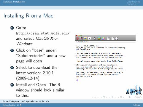
Installing R on a Mac

1 Go tohttp://cran.stat.ucla.edu/

and select MacOS X orWindows

2 Click on ”base” under”Subdirectories” and a newpage will open

3 Select to download thelatest version: 2.10.1(2009-12-14)

4 Install and Open. The Rwindow should look similarto this:





2 Generating from Distributions (Cont’d)Gamma DistributionBinomial Distribution




Gamma Distribution

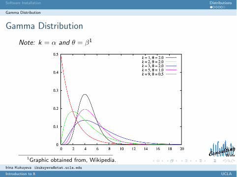
Gamma Distribution

Note: k = ! and " = #1

1Graphic obtained from, Wikipedia.Irina Kukuyeva [email protected]



Gamma Distribution

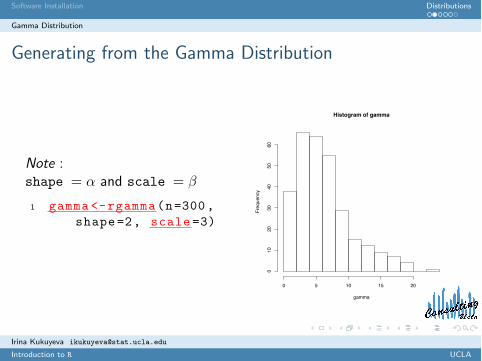
Generating from the Gamma Distribution

Note :shape = ! and scale = #

1 gamma <-rgamma(n=300,shape=2, scale =3)

Histogram of gamma

gamma

Frequency

0 5 10 15 20

010

2030

4050

60




Gamma Distribution

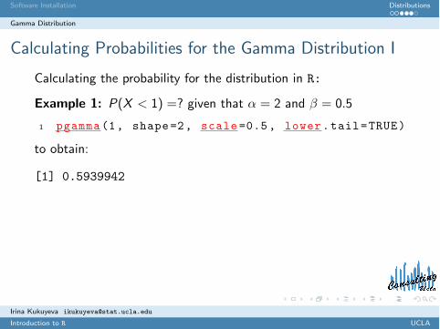
Calculating Probabilities for the Gamma Distribution I

Calculating the probability for the distribution in R:

Example 1: P(X < 1) =? given that ! = 2 and # = 0.5

1 pgamma(1, shape=2, scale =0.5, lower.tail=TRUE)

to obtain:

[1] 0.5939942




Gamma Distribution

Calculating Probabilities for the Gamma Distribution II

Example 2: P(X > 1) =? given that ! = 2 and # = 0.5

1 1-pgamma(1, shape=2, scale =0.5, lower.tail=TRUE)

2 # Alternatively:3 pgamma(1, shape=2, scale =0.5, lower.tail=FALSE

)

to obtain:

[1] 0.4060058




Gamma Distribution

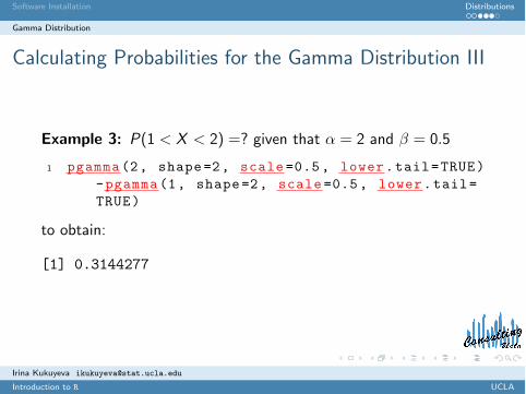
Calculating Probabilities for the Gamma Distribution III

Example 3: P(1 < X < 2) =? given that ! = 2 and # = 0.5

1 pgamma(2, shape=2, scale =0.5, lower.tail=TRUE)-pgamma(1, shape=2, scale =0.5, lower.tail=TRUE)

to obtain:

[1] 0.3144277




Binomial Distribution

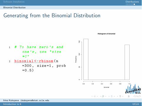
Generating from the Binomial Distribution

1 # To have zero ’s andone ’s, use "size=1"

2 binomial <-rbinom(n=300, size=1, prob=0.5)

Histogram of binomial

binomial

Frequency

0.0 0.2 0.4 0.6 0.8 1.0

050

100

150




Poisson Distribution

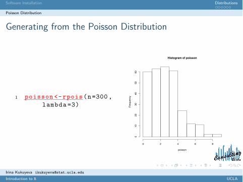
Generating from the Poisson Distribution

1 poisson <-rpois(n=300,lambda =3)

Histogram of poisson

poisson

Frequency

0 2 4 6 8

010

2030

4050

60



introduction to r - ucla statisticsnchristo/statistics100b/distributions1.pdf · software...

Documents