introduction to random variables 1 definition of random ... · introduction to random variables 1...
TRANSCRIPT

Estadística, Profesora: María Durbán1
Introduction to Random Variables
1 Definition of random variable
2 Discrete and continuous random variable
Probability function Distribution functionDensity function
3 Characteristic measures of a random variable
Mean, varianceOther measures
4 Transformation of random variables
Estadística, Profesora: María Durbán2
1 Definition of random variable
Sometimes, it is not enough to describe all possible results of an experiment:
Toss a coin 3 times: {(HHH), (HHT), …}Throw a dice twice: {(1,1), (1,2), (1,3), …}
Some tine it is useful to associate a number to each result of an experiment
Define a variable
We don’t know the result of the experiment before we carry it out We don’t know the value of the variable before the experiment
Estadística, Profesora: María Durbán3
1 Definition of random variable
A veces es útil asociar un número a cada resultado del experimento.
No conocemos el resultado del experimento antes de realizarlo
No conocemos el valor que va a tomar la variable antes del experimento
X = Number of head on the first toss X[(HHH)]=1, X[(THT)]=0, …
Y = Sum of points Y[(1,1)]=2, Y[(1,2)]=3, …
Sometimes, it is not enough to describe all possible results of an experiment:
Toss a coin 3 times: {(HHH), (HHT), …}Throw a dice twice: {(1,1), (1,2), (1,3), …}
Estadística, Profesora: María Durbán4
1 Definition of random variable
A random variable is a function which associates a real number to each element of the sample space
Random Variables are represented in capital letters, generallythe last letters of the alphabet: X,Y, Z, etc.
The values taken by the variable are represented by small letters,
x=1 is a possible value of X y=3.2 is a possible value of Yz=-7.3 is a possible value of Z
Estadística, Profesora: María Durbán5
1 Definition of random variable
Examples
Number of defective units in a random sample of 5 units
Number of faults per cm2 of material
Lifetime of a lamp
Resistance to compression of concrete
Estadística, Profesora: María Durbán6
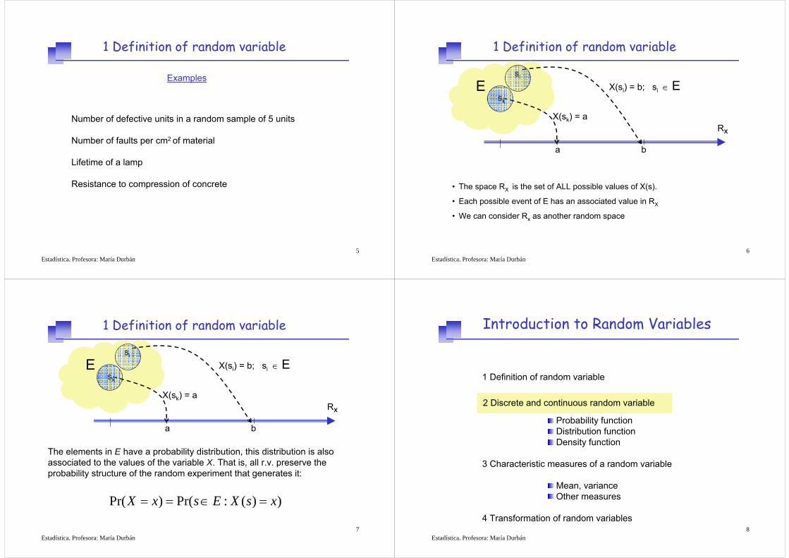
a b
RX
E X(si) = b; si ∈ E
X(sk) = a
si
sk
• The space RX is the set of ALL possible values of X(s).
• Each possible event of E has an associated value in RX
• We can consider Rx as another random space
1 Definition of random variable
Estadística, Profesora: María Durbán7
a b
RX
E X(si) = b; si ∈ E
X(sk) = a
si
sk
The elements in E have a probability distribution, this distribution is alsoassociated to the values of the variable X. That is, all r.v. preserve the probability structure of the random experiment that generates it:
Pr( ) Pr( : ( ) )X x s E X s x= = ∈ =
1 Definition of random variable
Estadística, Profesora: María Durbán8
Introduction to Random Variables
1 Definition of random variable
2 Discrete and continuos random variables
Probability functionDistribution functionDensity function
3 Characteristic measures of a random variable
Mean, varianceOther measures
4 Transformation of random variables
2 Discrete and continuous random variable
Estadística, Profesora: María Durbán9
2 Discrete and continuous random variables
The rank of a random variable una variable aleatoria is the set ofpossible values taken by the variable.
Depending on the rank, the variables can be classified as:
Discrete: Those that take a finite or infinite (numerable) number of values
Continuous: Those whose rank is an interval of real numbers
Discrete: Those that take a finite or infinite (numerable) number of values
Continuous: Those whose rank is an interval of real numbers
Estadística, Profesora: María Durbán10
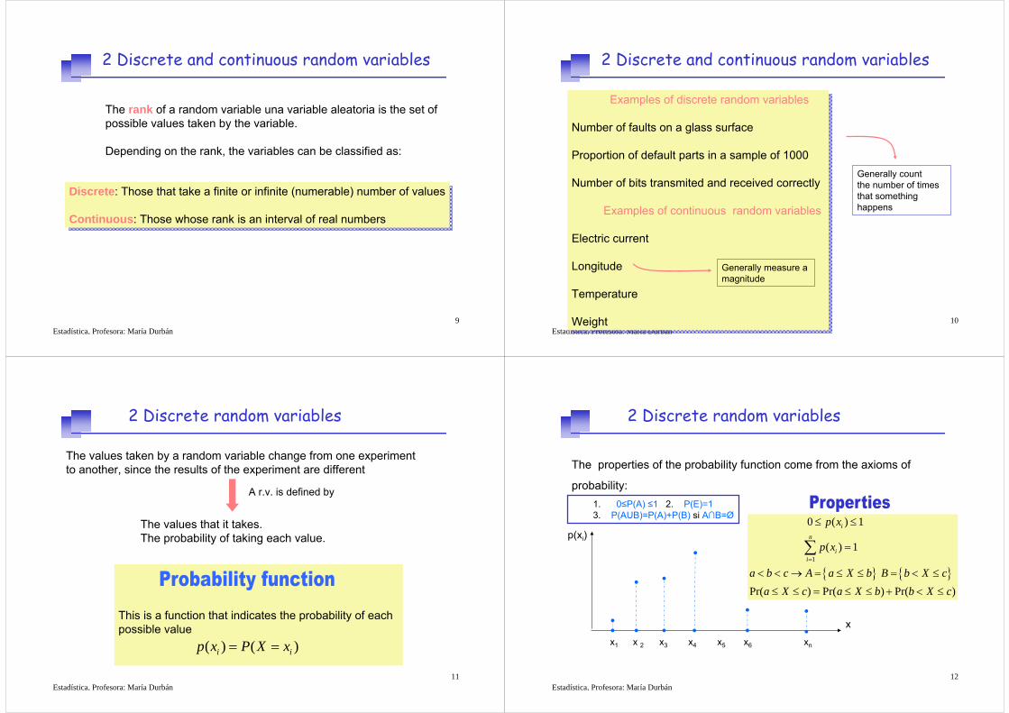
Examples of discrete random variables
Number of faults on a glass surface
Proportion of default parts in a sample of 1000
Number of bits transmited and received correctly
Examples of continuous random variables
Electric current
Longitude
Temperature
Weight
Examples of discrete random variables
Number of faults on a glass surface
Proportion of default parts in a sample of 1000
Number of bits transmited and received correctly
Examples of continuous random variables
Electric current
Longitude
Temperature
Weight
Generally count the number of times that somethinghappens
Generally measure a magnitude
2 Discrete and continuous random variables
Estadística, Profesora: María Durbán11
2 Discrete random variables
The values taken by a random variable change from one experimentto another, since the results of the experiment are different
A r.v. is defined by
The values that it takes.The probability of taking each value.
This is a function that indicates the probability of each possible value
( ) ( )i ip x P X x= =
Estadística, Profesora: María Durbán12
x
x1 x 2 x3 x4 x5 x6 xn
p(xi)
The properties of the probability function come from the axioms of
probability:
{ } { }1
0 ( ) 1
( ) 1
Pr( ) Pr( ) Pr( )
in
ii
p x
p x
a b c A a X b B b X ca X c a X b b X c
=
≤ ≤
=
< < → = ≤ ≤ = < ≤
≤ ≤ = ≤ ≤ + < ≤
∑
1. 0≤P(A) ≤1 2. P(E)=1 3. P(AUB)=P(A)+P(B) si A∩B=Ø
2 Discrete random variables
Estadística, Profesora: María Durbán13
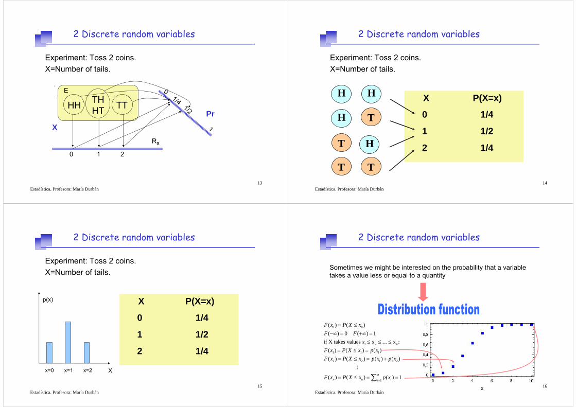
Experiment: Toss 2 coins. X=Number of tails.
HH THHT TT
RX
X
0 1 2
0 1/4 1/2 1
Pr
E
2 Discrete random variables
Estadística, Profesora: María Durbán14
X P(X=x)
0 1/4
1 1/2
2 1/4
T
T
T T
H H
H
H
Experiment: Toss 2 coins. X=Number of tails.
2 Discrete random variables
Estadística, Profesora: María Durbán15
X P(X=x)
0 1/4
1 1/2
2 1/4
x=0 x=1 x=2 X
p(x)
Experiment: Toss 2 coins. X=Number of tails.
2 Discrete random variables
Estadística, Profesora: María Durbán16
Sometimes we might be interested on the probability that a variable takes a value less or equal to a quantity
0 0
1 2 n
1 1 1
2 2 1 2
1
( ) ( )( ) 0 ( ) 1
if X takes values x x : ( ) ( ) ( )( ) ( ) ( ) ( )
( ) ( ) ( ) 1nn n ii
F x P X xF F
xF x P X x p xF x P X x p x p x
F x P X x p x=
= ≤−∞ = +∞ =
≤ ≤ ≤= ≤ == ≤ = +
= ≤ = =∑
K
M
2 Discrete random variables
Estadística, Profesora: María Durbán17
X P(X=x)
0 1/4
1 1/2
2 1/4
x=0 x=1 x=2 X
p(x)
Experiment: Toss 2 coins. X=Number of tails.
2 Discrete random variables
Estadística, Profesora: María Durbán18
X F(x)
0 1/4
1 3/4
2 1
x=0 x=1 x=2 X
F(x)
0.25
0.5
0.75
1
Experiment: Toss 2 coins. X=Number of tails.
2 Discrete random variables
Estadística, Profesora: María Durbán19
2 Continuous random variables
When a random variable is continuous, it doesn’t make sense to sum:
1( ) 1i
ip x
∞
=
=∑
Since the set of of values taken by the variable is not numerable
We can generalize
We introduce a new concept instead of the probability function of discrete random variables
→∑ ∫
Estadística, Profesora: María Durbán20
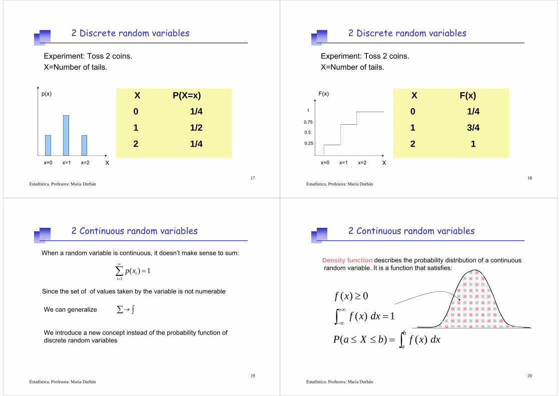
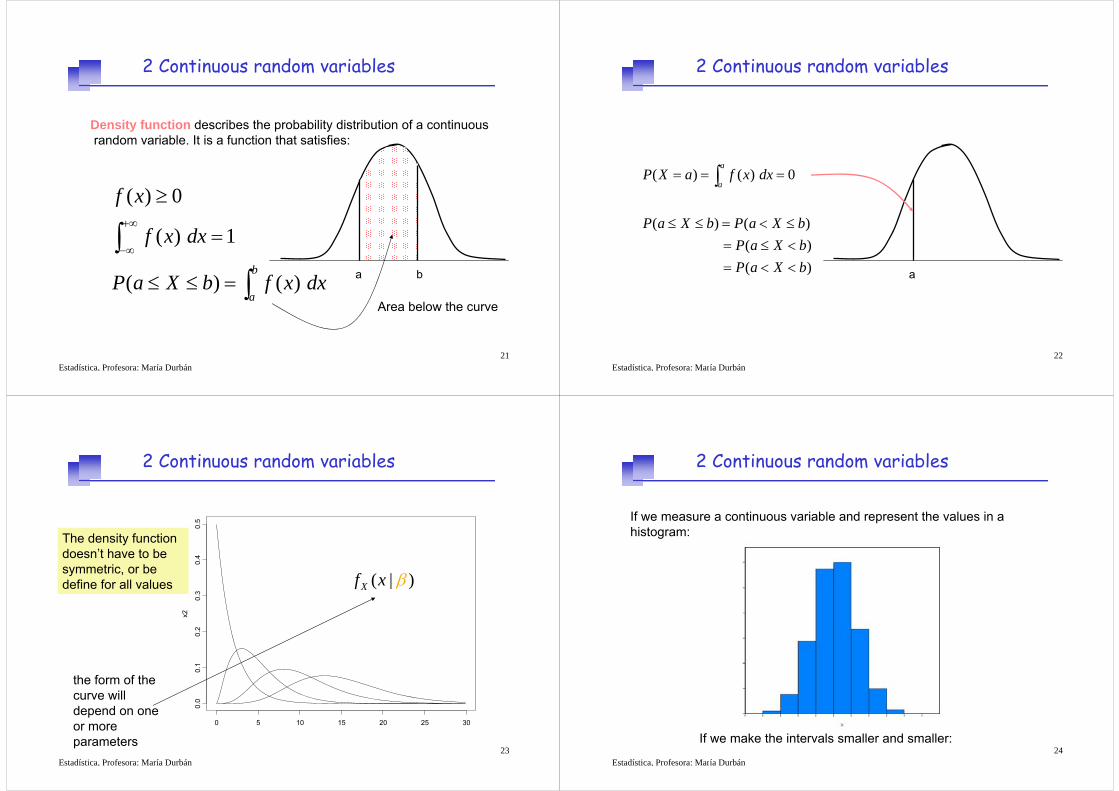
Density function describes the probability distribution of a continuousrandom variable. It is a function that satisfies:
( ) 0
( ) 1
( ) ( ) b
a
f x
f x dx
P a X b f x dx
+∞
−∞
≥
=
≤ ≤ =
∫∫
2 Continuous random variables
Estadística, Profesora: María Durbán21
( ) 0
( ) 1
( ) ( ) b
a
f x
f x dx
P a X b f x dx
+∞
−∞
≥
=
≤ ≤ =
∫∫ a b
Area below the curve
Density function describes the probability distribution of a continuousrandom variable. It is a function that satisfies:
2 Continuous random variables
Estadística, Profesora: María Durbán22
( ) ( ) 0
( ) ( ) ( ) ( )
a
aP X a f x dx
P a X b P a X bP a X bP a X b
= = =
≤ ≤ = < ≤= ≤ <= < <
∫
a
2 Continuous random variables
Estadística, Profesora: María Durbán23
y
x2
0 5 10 15 20 25 30
0.0
0.1
0.2
0.3
0.4
0.5
The density function doesn’t have to be symmetric, or be define for all values
the form of the curve will depend on one or more parameters
( | )Xf x β
2 Continuous random variables
Estadística, Profesora: María Durbán24
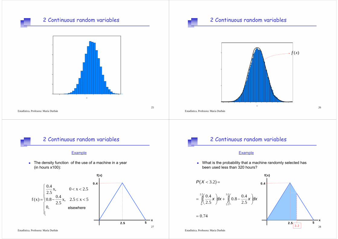
If we measure a continuous variable and represent the values in a histogram:
If we make the intervals smaller and smaller:
2 Continuous random variables
Estadística, Profesora: María Durbán25
2 Continuous random variables
Estadística, Profesora: María Durbán26
( )f x
2 Continuous random variables
Estadística, Profesora: María Durbán27
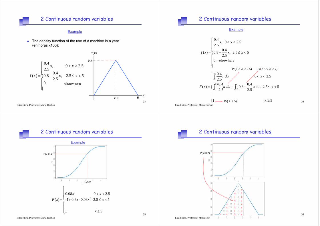
The density function of the use of a machine in a year (in hours x100):
⎪⎪⎪
⎩
⎪⎪⎪
⎨
⎧
<≤−
<<
=
else0,
5x2.5x,2.50.40.8
2.5x0x,2.50.4
)x(f
2.5 5
0.4
f(x)
x
Example
elsewhere
2 Continuous random variables
Estadística, Profesora: María Durbán28
What is the probability that a machine randomly selected has been used less than 320 hours?
2.5 5
0.4
f(x)
x
3.2
740
524080
5240
23
52
0
23
52
.
.
....
).(
. .
.
=
⎟⎠⎞
⎜⎝⎛ −+⎟
⎠⎞
⎜⎝⎛=
=<
∫ ∫ dxxdxx
XP
Example
2 Continuous random variables

29
As in the case of discrete random variables, we can define the distribution of a continuous random variables by means of the Distribution function:
( ) ( ) ( ) x
F x P X x f u du x−∞
= ≤ = −∞ < < ∞∫
x
( )P X x≤
2 Continuous random variables
Estadística, Profesora: María Durbán30
( ) ( ) ( ) x
F x P X x f u du x−∞
= ≤ = −∞ < < ∞∫
( )( ) dF xf xdx
=
In the discrete case, the Probability function is obtained as the difference of to adjoin values of F(x). In the case of continuous variables:
As in the case of discrete random variables, we can define the distribution of a continuous random variables by means of the Distribution function:
2 Continuous random variables
Estadística, Profesora: María Durbán31
The Distribution function satisfies the following properties:
( ) ( )( ) 0 ( ) 1
a b F a F bF F< ⇒ ≤−∞ = +∞ =
If we define the following disjoint events:
{ } { } { } { } { } X a a X b X a a X b X b≤ < ≤ → ≤ ∪ < ≤ = ≤
Pr( ) Pr( ) Pr( ) ( )X b X a a X b F b≤ = ≤ + < ≤ ≤
It is non-decreasingIt is right-continuous
Third axiom of probability
0≥
First axiom ofprobability
2 Continuous random variables
Estadística, Profesora: María Durbán32
( ) ( )( ) 0 ( ) 1
a b F a F bF F< ⇒ ≤−∞ = +∞ =
( ) Pr( ) ( ) 0
( ) Pr( ) ( ) 1
F X f x dx
F X f x dx
−∞
−∞
+∞
−∞
−∞ = ≤ −∞ = =
+∞ = ≤ +∞ = =
∫∫
The Distribution function satisfies the following properties:
2 Continuous random variables
Estadística, Profesora: María Durbán33
The density function of the use of a machine in a year (en horas x100):
⎪⎪⎪
⎩
⎪⎪⎪
⎨
⎧
<≤−
<<
=
else0,
5x2.5x,2.50.40.8
2.5x0x,2.50.4
)x(f
2.5 5
0.4
f(x)
x
Example
elsewhere
2 Continuous random variables
Estadística, Profesora: María Durbán34
Example
0
2.5
0 2.5
0.4 0 x 2.52.50.4 0.4( ) 0.8 u du, 2.5 x 52.5 2.5
1 x 5
x
x
u du
F x u du
⎧< <⎪
⎪⎪= + − ≤ <⎨⎪⎪⎪ ≥⎩
∫
∫ ∫
0.4 x, 0 x 2.52.5
0.4( ) 0.8 x, 2.5 x 52.5
0, elsewhere
f x
⎧ < <⎪⎪⎪= − ≤ <⎨⎪⎪⎪⎩
Pr(0 2.5)X< < Pr(2.5 )X x≤ <
Pr( 5)X ≤
2 Continuous random variables
Estadística, Profesora: María Durbán35
ExampleExample
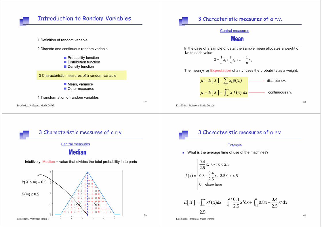
x=3.2
P(x<3.2)
2
2
0.08 0 2.5( ) -1 0.8 - 0.08 2.5 5
1 5
x xF x x x x
x
⎧⎪ < <⎪⎪= + ≤ <⎨⎪⎪
≥⎪⎩
2 Continuous random variables
Estadística, Profesora: María Durbán36
Example
P(x<3.2)
2 Continuous random variables
Estadística, Profesora: María Durbán37
Introduction to Random Variables
1 Definition of random variable
2 Discrete and continuous random variable
Probability functionDistribution functionDensity function
3 Characteristic measures of a random variable
Mean, varianceOther measures
4 Transformation of random variables
3 Characteristic measures of a random variable
Estadística, Profesora: María Durbán38
3 Characteristic measures of a r.v.
Central measures
In the case of a sample of data, the sample mean allocates a weight of 1/n to each value:
The mean or Expectation of a r.v. uses the probability as a weight:
1 21 1 1
nx x x xn n n
= + + +K
μ
[ ]
[ ]
( )
( )
i ii
E X x p x
E X x f x dx
μ
μ+∞
−∞
= =
= =
∑
∫
discrete r.v.
continuous r.v.
Estadística, Profesora: María Durbán39
3 Characteristic measures of a r.v.
Intuitively: Median = value that divides the total probability in to parts
0.50.5
( ) 0.5
( ) 0.5
P X m
F m
≤ =
≥
Central measures
Estadística, Profesora: María Durbán40
What is the average time of use of the machines?
Example
[ ]2.5 52 2
0 2.5
0.4 0.4( ) d 0.8 d2.5 2.5
2.5
E X xf x dx x x x x x+∞
−∞= = + −
=
∫ ∫ ∫
0.4 x, 0 x 2.52.5
0.4( ) 0.8 x, 2.5 x 52.5
0, elsewhere
f x
⎧ < <⎪⎪⎪= − ≤ <⎨⎪⎪⎪⎩
3 Characteristic measures of a r.v.

Estadística, Profesora: María Durbán41
If we want to know the time of use such that 50% of the machineshave a use less or equal to that value
Example
( ) 0.5F m =2
2
0.08 0 x 2.5( ) -1 0.8 - 0.08 2.5 x 5
1 x 5
xF x x x
⎧ < <⎪= + ≤ <⎨⎪ ≥⎩
2
2
0.08 0.5 2.5-1 0.8 - 0.08 0.5 2.5
x mx x m= → =
+ = → =
3 Characteristic measures of a r.v.
Estadística, Profesora: María Durbán42
3 Characteristic measures of a r.v.
Other measures
The percentil p of a random variable is the value xp that satisfies:
( ) y ( )( )
p p
p
p X x p p X x pF x p
< ≤ ≤ ≥
=discrete r.v.
continuous r.v.
A special case are quartiles which divide the distribution in 4 parts
1 0.25
2 0.5
3 0.75
MedianQ pQ pQ p
== ==
Estadística, Profesora: María Durbán43
3 Characteristic measures of a r.v.
Medisures of dispersion
The sample variance of a set of data is given by:
The Variance of a r.v. also uses the probability as a weight:
2 2 2 21 2
1 1 1( ) ( ) ( )ns x x x x x xn n n
= − + − + + −K
[ ]
[ ]
22
2 2
( ) ( )
( ) ( )
i ii
Var X x p x
Var X x f x dx
σ μ
σ μ+∞
−∞
= = −
= = −
∑
∫
discrete r.v.
continuous r.v.
[ ] [ ]( )2Var X E X E X⎡ ⎤= −
⎣ ⎦
Estadística, Profesora: María Durbán44
3 Characteristic measures of a r.v.
[ ] [ ]( )2Var X E X E X⎡ ⎤= −
⎣ ⎦
[ ] [ ]( )22Var X E X E X⎡ ⎤= −⎣ ⎦
[ ]( ) [ ]( ) [ ]
[ ]( ) [ ] [ ]
[ ]( )
2 22
22
22
2
2
E X E X E X E X XE X
E X E X E X E X
E X E X
⎡ ⎤ ⎡ ⎤− = + −⎣ ⎦ ⎣ ⎦
⎡ ⎤= + −⎣ ⎦
⎡ ⎤= −⎣ ⎦ It is a linear operator
[ ] is a constant, does not depend on E X
X
Medisures of dispersion
Estadística, Profesora: María Durbán45
Introduction to Random Variables
1 Definition of random variable
2 Discrete and continuous random variable
Probability functionDistribution functionDensity function
3 Characteristic measures of a random variable
Mean, varianceOther measures
4 Transformation of random variables4 Transformation of random variables
Estadística, Profesora: María Durbán46
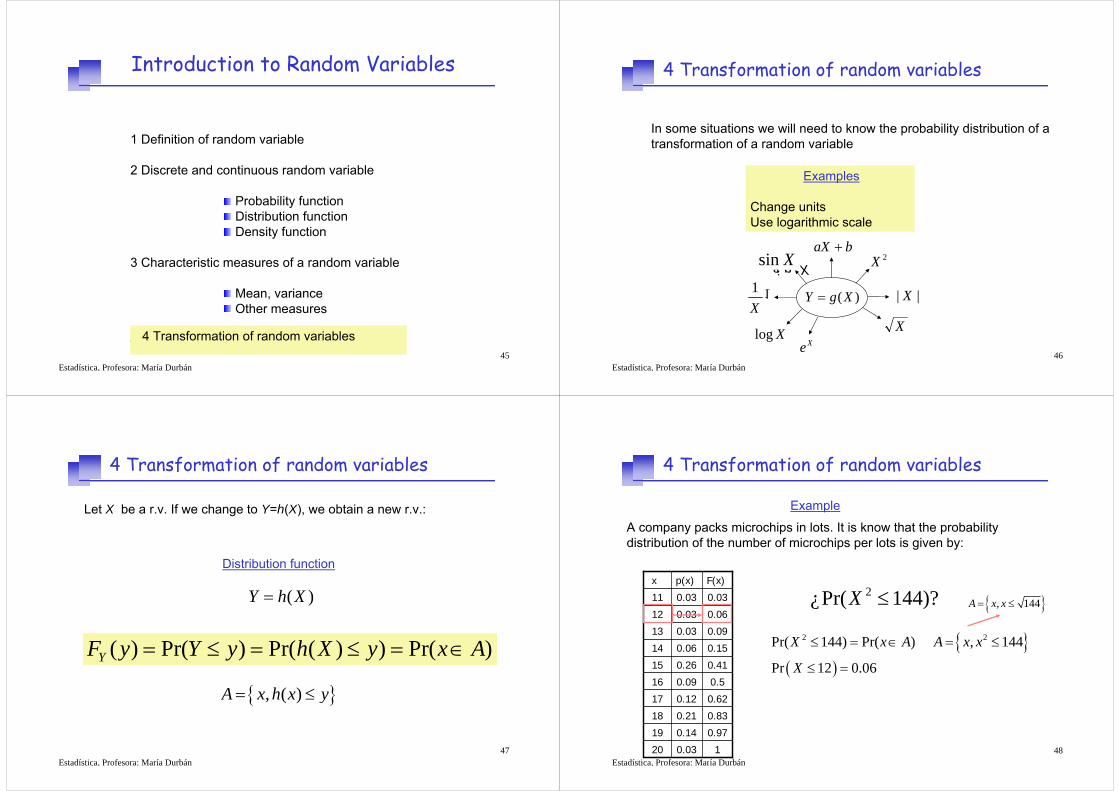
4 Transformation of random variables
In some situations we will need to know the probability distribution of atransformation of a random variable
Examples
Change unitsUse logarithmic scale
)(XgY =
baX +2X
|| X
XXe
XlogX
1nis X sin X
1X
Estadística, Profesora: María Durbán47
4 Transformation of random variables
Let X be a r.v. If we change to Y=h(X), we obtain a new r.v.:
( ) Pr( ) Pr( ( ) ) Pr( )YF y Y y h X y x A= ≤ = ≤ = ∈
( )Y h X=
{ }, ( )A x h x y= ≤
Distribution function
Estadística, Profesora: María Durbán48
Example
A company packs microchips in lots. It is know that the probabilitydistribution of the number of microchips per lots is given by:
0.03
0.14
0.21
0.12
0.09
0.26
0.06
0.03
0.03
0.03
p(x)
1
0.97
0.83
0.62
0.5
0.41
0.15
0.09
0.06
0.03
F(x)
20
19
18
17
16
15
14
13
12
11
x2¿Pr( 144)?X ≤
{ }( )
2 2Pr( 144) Pr( ) , 144
Pr 12 0.06
X x A A x x
X
≤ = ∈ = ≤
≤ =
4 Transformation of random variables
{ }, 144A x x= ≤
Estadística, Profesora: María Durbán49
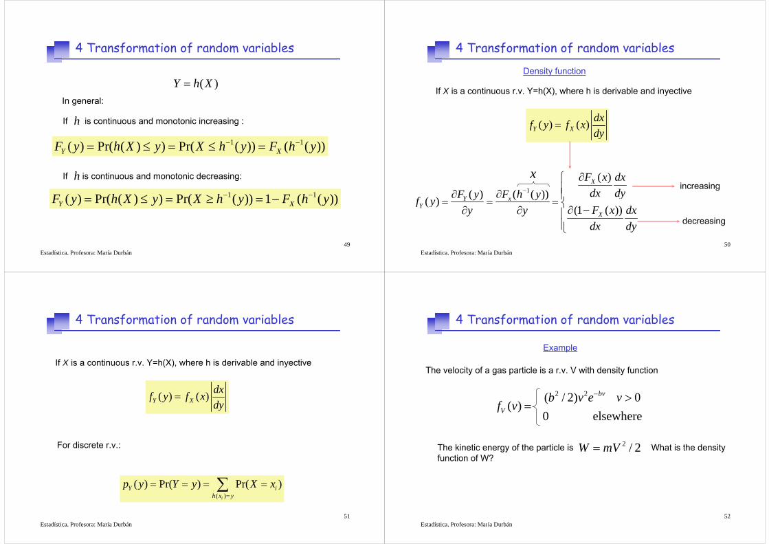
4 Transformation of random variables
1 1( ) Pr( ( ) ) Pr( ( )) ( ( ))Y XF y h X y X h y F h y− −= ≤ = ≤ =
( )Y h X=In general:
If is continuous and monotonic increasing :h
If is continuous and monotonic decreasing:h1 1( ) Pr( ( ) ) Pr( ( )) 1 ( ( ))Y XF y h X y X h y F h y− −= ≤ = ≥ = −
Estadística, Profesora: María Durbán50
4 Transformation of random variables
If X is a continuous r.v. Y=h(X), where h is derivable and inyective
( ) ( )Y Xdxf y f xdy
=
Density function
1
( )( ( ))( )( )
(1 ( ))
X
xYY
X
F x dxdx dyF h yF yf yF x dxy ydx dy
−
∂⎧⎪∂∂ ⎪= = = ⎨∂ −∂ ∂ ⎪⎪⎩
increasing
decreasing
x
Estadística, Profesora: María Durbán51
4 Transformation of random variables
For discrete r.v.:
( )( ) Pr( ) Pr( )
i
Y ih x y
p y Y y X x=
= = = =∑
( ) ( )Y Xdxf y f xdy
=
If X is a continuous r.v. Y=h(X), where h is derivable and inyective
Estadística, Profesora: María Durbán52
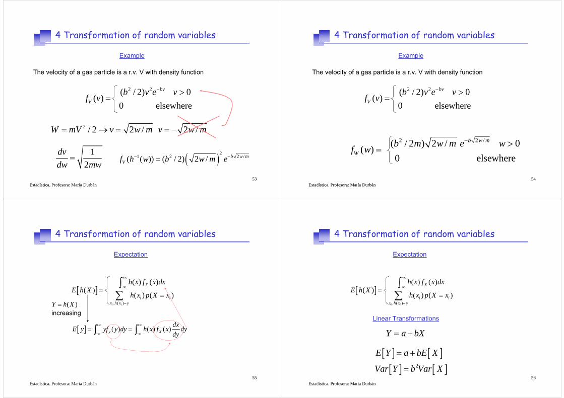
4 Transformation of random variables
Example
The velocity of a gas particle is a r.v. V with density function
2 2( / 2) 0( )
0 elsewhere
bv
Vb v e v
f v− >
=
The kinetic energy of the particle is What is the density function of W?
2 / 2W mV=
Estadística, Profesora: María Durbán53
4 Transformation of random variables
Example
2 2( / 2) 0( )
0 elsewhere
bv
Vb v e v
f v− >
=
2 / 2 2 / 2 /W mV v w m v w m= → = = −
12
dvdw mw
= ( )21 2 2 /( ( )) ( / 2) 2 / b w m
Vf h w b w m e− −=
The velocity of a gas particle is a r.v. V with density function
Estadística, Profesora: María Durbán54
4 Transformation of random variables
Example
2 2( / 2) 0( )
0 elsewhere
bv
Vb v e v
f v− >
=
2 2 /( / 2 ) 2 / 0( ) 0 elsewhere
b w m
Wb m w m e wf w
− >=
The velocity of a gas particle is a r.v. V with density function
Estadística, Profesora: María Durbán55
4 Transformation of random variables
Expectation
[ ], ( )
( ) ( )( )
( ) ( )i i
X
i ix h x y
h x f x dxE h X
h x p X x
+∞
−∞
=
==
∫∑
[ ] ( ) ( ) ( )y XdxE y yf y dy h x f x dydy
+∞ +∞
−∞ −∞= =∫ ∫
( )Y h X=increasing
Estadística, Profesora: María Durbán56
4 Transformation of random variables
Expectation
[ ], ( )
( ) ( )( )
( ) ( )i i
X
i ix h x y
h x f x dxE h X
h x p X x
+∞
−∞
=
==
∫∑
Linear Transformations
Y a bX= +
[ ] [ ][ ] [ ]2
E Y a bE X
Var Y b Var X
= +
=