introduction to regression in r part i : simple linear...

Preliminaries Introduction Simple Linear Regression Resources References Upcoming Survey Questions Exercises

UCLA Department of StatisticsStatistical Consulting Center

Introduction to Regression in RPart I :

Simple Linear Regression

Denise [email protected]

May 5, 2009

Denise Ferrari [email protected]

Regression in R I UCLA SCC


Outline

1 Preliminaries

2 Introduction

3 Simple Linear Regression

4 Online Resources for R

5 References

6 Upcoming Mini-Courses

7 Feedback Survey

8 Questions

9 ExercisesDenise Ferrari [email protected]



1 PreliminariesObjectiveSoftware InstallationR HelpImporting Data Sets into R

Importing Data from the InternetImporting Data from Your ComputerUsing Data Available in R

2 Introduction



5 References


7 Feedback Survey

8 Questions

9 Exercises




Objective

Objective

The main objective of this mini-course is to show how to performRegression Analysis in R.Prior knowledge of the basics of Linear Regression Models isassumed.




Software Installation

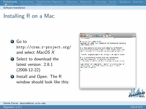
Installing R on a Mac

1 Go tohttp://cran.r-project.org/

and select MacOS X

2 Select to download thelatest version: 2.8.1(2008-12-22)

3 Install and Open. The Rwindow should look like this:




R Help

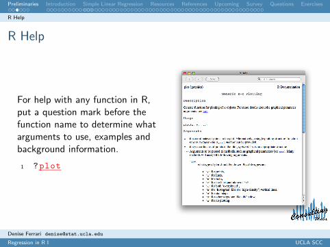
R Help

For help with any function in R,put a question mark before thefunction name to determine whatarguments to use, examples andbackground information.

1 ?plot




Importing Data Sets into R

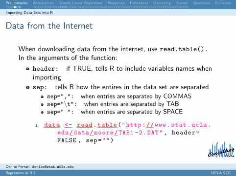
Data from the Internet

When downloading data from the internet, use read.table().In the arguments of the function:

header: if TRUE, tells R to include variables names whenimporting

sep: tells R how the entires in the data set are separated

sep=",": when entries are separated by COMMASsep="\t": when entries are separated by TABsep=" ": when entries are separated by SPACE

1 data <- read.table("http://www.stat.ucla.edu/data/moore/TAB1 -2. DAT", header=FALSE , sep="")





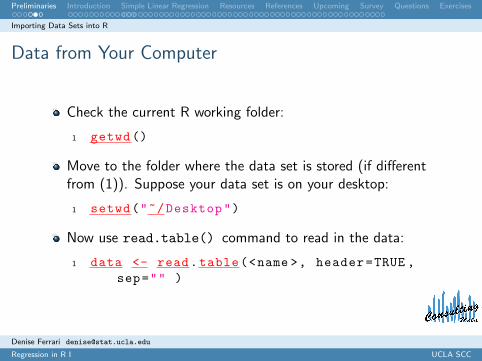
Data from Your Computer

Check the current R working folder:

1 getwd ()

Move to the folder where the data set is stored (if differentfrom (1)). Suppose your data set is on your desktop:

1 setwd("~/Desktop")

Now use read.table() command to read in the data:

1 data <- read.table(<name >, header=TRUE ,sep="" )





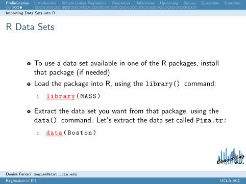
R Data Sets

To use a data set available in one of the R packages, installthat package (if needed).

Load the package into R, using the library() command:

1 library(MASS)

Extract the data set you want from that package, using thedata() command. Let’s extract the data set called Pima.tr:

1 data(Boston)




1 Preliminaries

2 IntroductionWhat is Regression?Initial Data Analysis

Numerical SummariesGraphical Summaries



5 References


7 Feedback Survey

8 Questions

9 Exercises




What is Regression?

When to Use Regression Analysis?

Regression analysis is used to describe the relationship between:

A single response variable: Y ; and

One or more predictor variables: X1,X2, . . . ,Xp

− p = 1: Simple Regression− p > 1: Multivariate Regression




What is Regression?

The Variables

Response Variable

The response variable Y must be a continuous variable.

Predictor Variables

The predictors X1, . . . ,Xp can be continuous, discrete orcategorical variables.




Initial Data Analysis

Initial Data Analysis IDoes the data look like as we expect?

Prior to any analysis, the data should always be inspected for:

Data-entry errors

Missing values

Outliers

Unusual (e.g. asymmetric) distributions

Changes in variability

Clustering

Non-linear bivariate relatioships

Unexpected patterns





Initial Data Analysis IIDoes the data look like as we expect?

We can resort to:

Numerical summaries:

− 5-number summaries− correlations− etc.

Graphical summaries:

− boxplots− histograms− scatterplots− etc.





Loading the DataExample: Diabetes in Pima Indian Women 1

Clean the workspace using the command: rm(list=ls())Download the data from the internet:

1 pima <- read.table("http://archive.ics.uci.edu/ml/machine -learning -databases/pima -indians -diabetes/pima -indians -diabetes.data", header=F, sep=",")

Name the variables:

1 colnames(pima) <- c("npreg", "glucose","bp", "triceps", "insulin", "bmi", "diabetes", "age", "class")

1Data from the UCI Machine Learning Repositoryhttp://archive.ics.uci.edu/ml/machine-learning-databases/pima-indians-diabetes/

pima-indians-diabetes.names



http://archive.ics.uci.edu/ml/machine-learning-databases/pima-indians-diabetes/pima-indians-diabetes.names

http://archive.ics.uci.edu/ml/machine-learning-databases/pima-indians-diabetes/pima-indians-diabetes.names



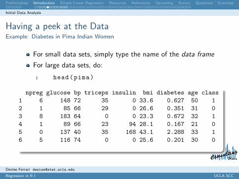
Having a peek at the DataExample: Diabetes in Pima Indian Women

For small data sets, simply type the name of the data frame

For large data sets, do:

1 head(pima)

npreg glucose bp triceps insulin bmi diabetes age class1 6 148 72 35 0 33.6 0.627 50 12 1 85 66 29 0 26.6 0.351 31 03 8 183 64 0 0 23.3 0.672 32 14 1 89 66 23 94 28.1 0.167 21 05 0 137 40 35 168 43.1 2.288 33 16 5 116 74 0 0 25.6 0.201 30 0





Numerical SummariesExample: Diabetes in Pima Indian Women

Univariate summary information:

− Look for unusual features in the data (data-entry errors,outliers): check, for example, min, max of each variable

1 summary(pima)

npreg glucose bp triceps insulin

Min. : 0.000 Min. : 0.0 Min. : 0.0 Min. : 0.00 Min. : 0.0

1st Qu.: 1.000 1st Qu.: 99.0 1st Qu.: 62.0 1st Qu.: 0.00 1st Qu.: 0.0

Median : 3.000 Median :117.0 Median : 72.0 Median :23.00 Median : 30.5

Mean : 3.845 Mean :120.9 Mean : 69.1 Mean :20.54 Mean : 79.8

3rd Qu.: 6.000 3rd Qu.:140.2 3rd Qu.: 80.0 3rd Qu.:32.00 3rd Qu.:127.2

Max. :17.000 Max. :199.0 Max. :122.0 Max. :99.00 Max. :846.0

bmi diabetes age class

Min. : 0.00 Min. :0.0780 Min. :21.00 Min. :0.0000

1st Qu.:27.30 1st Qu.:0.2437 1st Qu.:24.00 1st Qu.:0.0000

Median :32.00 Median :0.3725 Median :29.00 Median :0.0000

Mean :31.99 Mean :0.4719 Mean :33.24 Mean :0.3490

3rd Qu.:36.60 3rd Qu.:0.6262 3rd Qu.:41.00 3rd Qu.:1.0000

Max. :67.10 Max. :2.4200 Max. :81.00 Max. :1.0000

Categorical





Coding Missing Data IExample: Diabetes in Pima Indian Women

Variable “npreg” has maximum value equal to 17

− unusually large but not impossible

Variables “glucose”, “bp”, “triceps”, “insulin” and “bmi”have minimum value equal to zero

− in this case, it seems that zero was used to code missing data





Coding Missing Data IIExample: Diabetes in Pima Indian Women

R code for missing data

Zero should not be used to represent missing data

− it’s a valid value for some of the variables− can yield misleading results

Set the missing values coded as zero to NA:

1 pima$glucose[pima$glucose ==0] <- NA2 pima$bp[pima$bp==0] <- NA3 pima$triceps[pima$triceps ==0] <- NA4 pima$insulin[pima$insulin ==0] <- NA5 pima$bmi[pima$bmi ==0] <- NA





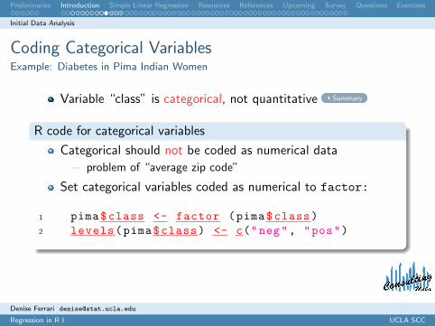
Coding Categorical VariablesExample: Diabetes in Pima Indian Women

Variable “class” is categorical, not quantitative Summary

R code for categorical variables

Categorical should not be coded as numerical data

− problem of “average zip code”

Set categorical variables coded as numerical to factor:

1 pima$class <- factor (pima$class)2 levels(pima$class) <- c("neg", "pos")





Final CodingExample: Diabetes in Pima Indian Women

1 summary(pima)

npreg glucose bp triceps insulin

Min. : 0.000 Min. : 44.0 Min. : 24.0 Min. : 7.00 Min. : 14.00

1st Qu.: 1.000 1st Qu.: 99.0 1st Qu.: 64.0 1st Qu.: 22.00 1st Qu.: 76.25

Median : 3.000 Median :117.0 Median : 72.0 Median : 29.00 Median :125.00

Mean : 3.845 Mean :121.7 Mean : 72.4 Mean : 29.15 Mean :155.55

3rd Qu.: 6.000 3rd Qu.:141.0 3rd Qu.: 80.0 3rd Qu.: 36.00 3rd Qu.:190.00

Max. :17.000 Max. :199.0 Max. :122.0 Max. : 99.00 Max. :846.00

NA’s : 5.0 NA’s : 35.0 NA’s :227.00 NA’s :374.00

bmi diabetes age class

Min. :18.20 Min. :0.0780 Min. :21.00 neg:500

1st Qu.:27.50 1st Qu.:0.2437 1st Qu.:24.00 pos:268

Median :32.30 Median :0.3725 Median :29.00

Mean :32.46 Mean :0.4719 Mean :33.24

3rd Qu.:36.60 3rd Qu.:0.6262 3rd Qu.:41.00

Max. :67.10 Max. :2.4200 Max. :81.00

NA’s :11.00





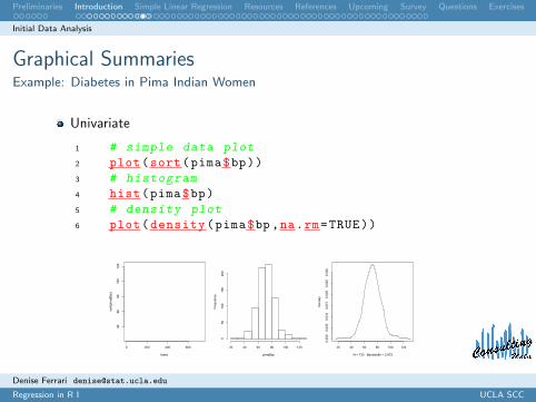
Graphical SummariesExample: Diabetes in Pima Indian Women

Univariate

1 # simple data plot

2 plot(sort(pima$bp))3 # histogram

4 hist(pima$bp)5 # density plot

6 plot(density(pima$bp ,na.rm=TRUE))

0 200 400 600

4060

80100

120

Index

sort(pima$bp)

pima$bp

Frequency

20 40 60 80 100 120

050

100

150

200

20 40 60 80 100 120

0.000

0.005

0.010

0.015

0.020

0.025

0.030

N = 733 Bandwidth = 2.872

Density





Graphical SummariesExample: Diabetes in Pima Indian Women

Bivariate

1 # scatterplot

2 plot(triceps~bmi , pima)3 # boxplot

4 boxplot(diabetes~class , pima)

20 30 40 50 60

2040

6080

100

bmi

triceps

neg pos

0.0

0.5

1.0

1.5

2.0

2.5

class

diabetes




1 Preliminaries

2 Introduction

3 Simple Linear RegressionSimple Linear Regression ModelEstimation and Inference

ANOVAGoodness of Fit

PredictionDummy VariablesDiagnostics

Diagnostic Plots

TransformationsTransformations


5 References


7 Feedback Survey

8 Questions

9 Exercises




Simple Linear Regression Model

Linear regression with a single predictor

Objective

Describe the relationship between two variables, say X and Y as astraight line, that is, Y is modeled as a linear function of X .

The variables

X : explanatory variable (horizontal axis)Y : response variable (vertical axis)

After data collection, we have pairs of observations:

(x1, y1), . . . , (xn, yn)





Linear regression with a single predictorExample: Production Runs (Taken from Sheather, 2009)

Loading the Data:

1 production <- read.table("http://www.stat.tamu.edu/~sheather/book/docs/datasets/production.txt", header=T, sep="")

Case RunTime RunSize

1 195 175

2 215 189

3 243 344

4 162 88

5 185 114

...

18 230 337

19 208 146

20 172 68

Variables:

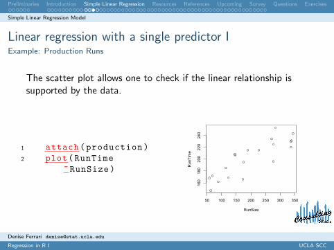
RunTime (Y ): time taken(in minutes) for a production run

RunSize (X ): number of items produced ineach run

We want to be able to describe theproduction run time as a linear function ofthe number of items in the run





Linear regression with a single predictor IExample: Production Runs

The scatter plot allows one to check if the linear relationship issupported by the data.

1 attach(production)2 plot(RunTime

~RunSize)

50 100 150 200 250 300 350160

180

200

220

240

RunSize

RunTime





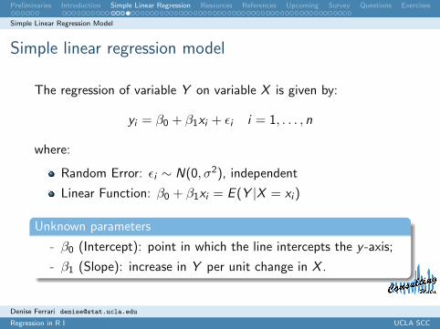
Simple linear regression model

The regression of variable Y on variable X is given by:

yi = β0 + β1xi + εi i = 1, . . . , n

where:

Random Error: εi ∼ N(0, σ2), independent

Linear Function: β0 + β1xi = E (Y |X = xi )

Unknown parameters

- β0 (Intercept): point in which the line intercepts the y -axis;

- β1 (Slope): increase in Y per unit change in X .




Estimation and Inference

Estimation of unknown parameters I

We want to find the equation of the line that “best” fits the data.It means finding b0 and b1 such that the fitted values of yi , givenby

yi = b0 + b1xi ,

are as “close” as possible to the observed values yi .

Residuals

The difference between theobserved value yi and the fittedvalue yi is called residual and isgiven by:ei = yi − yi





Estimation of unknown parameters II

Least Squares Method

A usual way of calculating b0 and b1 is based on the minimizationof the sum of the squared residuals, or residual sum of squares(RSS):

RSS =∑

i

e2i

=∑

i

(yi − yi )2

=∑

i

(yi − b0 − b1xi )2





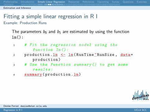
Fitting a simple linear regression in R IExample: Production Runs

The parameters b0 and b1 are estimated by using the functionlm():

1 # Fit the regression model using the

function lm():

2 production.lm <- lm(RunTime~RunSize , data=production)

3 # Use the function summary () to get some

results:

4 summary(production.lm)





Fitting a simple linear regression in R IIExample: Production Runs

The output looks like this:

Call:

lm(formula = RunTime ~ RunSize, data = production)

Residuals:

Min 1Q Median 3Q Max

-28.597 -11.079 3.329 8.302 29.627

Coefficients:

Estimate Std. Error t value Pr(>|t|)

(Intercept) 149.74770 8.32815 17.98 6.00e-13 ***

RunSize 0.25924 0.03714 6.98 1.61e-06 ***

---

Signif. codes: 0 *** 0.001 ** 0.01 * 0.05 . 0.1 1

Residual standard error: 16.25 on 18 degrees of freedom

Multiple R-squared: 0.7302, Adjusted R-squared: 0.7152

F-statistic: 48.72 on 1 and 18 DF, p-value: 1.615e-06

50 100 150 200 250 300 350

160

180

200

220

240

RunSizeRunTime





Fitted values and residuals

Fitted values obtained using the function fitted()Residuals obtained using the function resid()

1 # Create a table with fitted values and

residuals

2 data.frame(production , fitted.value=fitted(production.lm), residual=resid(production.lm))

Case RunTime RunSize fitted.value residual

1 195 175 195.1152 -0.1152469

2 215 189 198.7447 16.2553496

3 243 344 238.9273 4.0726679

...

20 172 68 167.3762 4.6237657

y1 = 149.75 + 0.26 ∗ 175 = 195.115e1 = 195 − 195.115 = −0.115





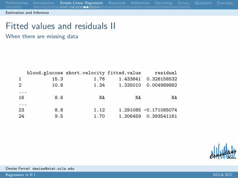
Fitted values and residuals IWhen there are missing data

Missing data need to be handled carefully. Using the na.excludemethod:

1 # Load the package that contains the data

2 library(ISwR)3 data(thuesen); attach(thuesen)4 # Option for dealing with missing data

5 options(na.action=na.exclude)6 # Now fit the regression model as before

7 velocity.lm <- lm(short.velocity~blood.glucose)

8 # Create a table with fitted values and

residuals

9 data.frame(thuesen , fitted.value=fitted(velocity.lm), residual=resid(velocity.lm))





Fitted values and residuals IIWhen there are missing data

blood.glucose short.velocity fitted.value residual

1 15.3 1.76 1.433841 0.326158532

2 10.8 1.34 1.335010 0.004989882

...

16 8.6 NA NA NA

...

23 8.8 1.12 1.291085 -0.171085074

24 9.5 1.70 1.306459 0.393541161





Analysis of Variance (ANOVA) I

The ANOVA breaks the total variability observed in the sampleinto two parts:

Total Variability Unexplainedsample = explained + (or error)variability by the model variability(TSS) (SSreg) (RSS)





Analysis of Variance (ANOVA) II

In R, we do:

1 anova(production.lm)

Analysis of Variance Table

Response: RunTimeDf Sum Sq Mean Sq F value Pr(>F)

RunSize 1 12868.4 12868.4 48.717 1.615e-06Residuals 18 4754.6 264.1





Measuring Goodness of Fit I

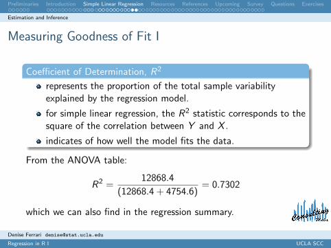
Coefficient of Determination, R2

represents the proportion of the total sample variabilityexplained by the regression model.

for simple linear regression, the R2 statistic corresponds to thesquare of the correlation between Y and X .

indicates of how well the model fits the data.

From the ANOVA table:

R2 =12868.4

(12868.4 + 4754.6)= 0.7302

which we can also find in the regression summary.





Measuring Goodness of Fit II

Adjusted R2

The adjusted R2 takes into account the number of degrees offreedom and is preferable to R2.

From the ANOVA table:

R2adj = 1− 4754.6/18

(12868.4 + 4754.6)/(18 + 1)= 0.7152

also found in the regression summary.

Attention

Neither R2 nor R2adj give direct indication on how well the model

will perform in the prediction of a new observation.




Prediction

Confidence and prediction bands I

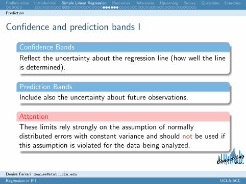
Confidence Bands

Reflect the uncertainty about the regression line (how well the lineis determined).

Prediction Bands

Include also the uncertainty about future observations.

Attention

These limits rely strongly on the assumption of normallydistributed errors with constant variance and should not be used ifthis assumption is violated for the data being analyzed.




Prediction

Confidence and prediction bands II

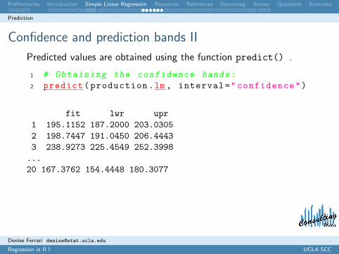
Predicted values are obtained using the function predict() .

1 # Obtaining the confidence bands:

2 predict(production.lm, interval="confidence")

fit lwr upr1 195.1152 187.2000 203.03052 198.7447 191.0450 206.44433 238.9273 225.4549 252.3998

...20 167.3762 154.4448 180.3077




Prediction

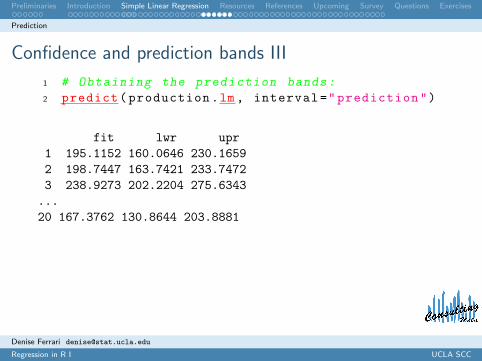
Confidence and prediction bands III

1 # Obtaining the prediction bands:

2 predict(production.lm, interval="prediction")

fit lwr upr1 195.1152 160.0646 230.16592 198.7447 163.7421 233.74723 238.9273 202.2204 275.6343

...20 167.3762 130.8644 203.8881




Prediction

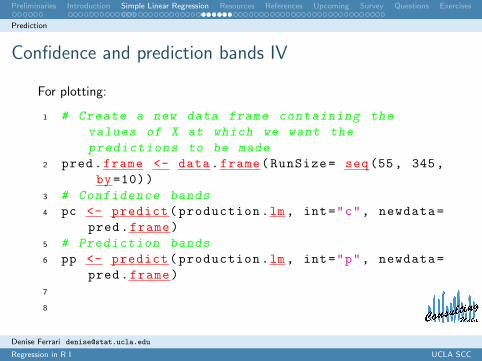
Confidence and prediction bands IV

For plotting:

1 # Create a new data frame containing the

values of X at which we want the

predictions to be made

2 pred.frame <- data.frame(RunSize= seq(55, 345,by=10))

3 # Confidence bands

4 pc <- predict(production.lm, int="c", newdata=pred.frame)

5 # Prediction bands

6 pp <- predict(production.lm, int="p", newdata=pred.frame)

7

8




Prediction

Confidence and prediction bands V

9 # Plot

10 require(graphics)11 # Standard scatterplot with extended limits

12 plot(RunSize , RunTime , ylim=range(RunSize , pp,na.rm=T))

13 pred.Size <- pred.frame$RunSize14 # Add curves

15 matlines(pred.Size , pc, lty=c(1,2,2), lwd=1.5,col =1)

16 matlines(pred.Size , pp, lty=c(1,3,3), lwd=1.5,col =1)




Prediction

Confidence and prediction bands VI

50 100 150 200 250 300 350

50100

150

200

250

300

350

RunSize

RunTime




Dummy Variables

Dummy Variable Regression

The simple dummy variable regression is used when the predictorvariable is not quantitative but categorical and assumes only twovalues.




Dummy Variables

Dummy Variable Regression IExample: Change over time (Taken from Sheather, 2009)

Loading the Data:

1 changeover <- read.table("http://www.stat.tamu.edu/~sheather/book/docs/datasets/changeover_times.txt", header=T, sep="")

Method Changeover New

1 Existing 19 0

2 Existing 24 0

3 Existing 39 0

...

118 New 14 1

119 New 40 1

120 New 35 1

Variables:

Change-over(Y ): time (in minutes)required to change the line of foodproduction

New (X ): 1 for the new method, 0 for theexisting method

We want to be able to test whether thechange-over time is different for the twomethods.




Dummy Variables

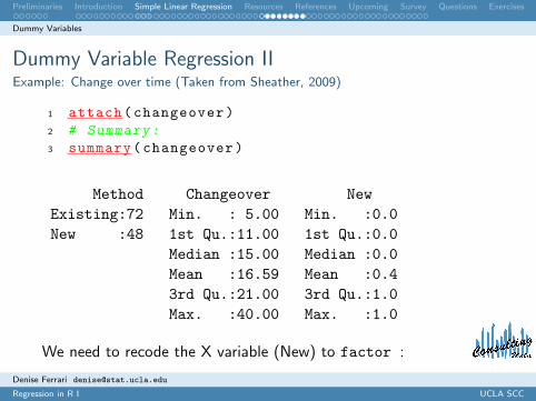
Dummy Variable Regression IIExample: Change over time (Taken from Sheather, 2009)

1 attach(changeover)2 # Summary:

3 summary(changeover)

Method Changeover NewExisting:72 Min. : 5.00 Min. :0.0New :48 1st Qu.:11.00 1st Qu.:0.0

Median :15.00 Median :0.0Mean :16.59 Mean :0.43rd Qu.:21.00 3rd Qu.:1.0Max. :40.00 Max. :1.0

We need to recode the X variable (New) to factor :




Dummy Variables

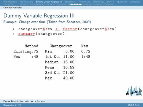
Dummy Variable Regression IIIExample: Change over time (Taken from Sheather, 2009)

1 changeover$New <- factor(changeover$New)2 summary(changeover)

Method Changeover NewExisting:72 Min. : 5.00 0:72New :48 1st Qu.:11.00 1:48

Median :15.00Mean :16.593rd Qu.:21.00Max. :40.00




Dummy Variables

Dummy Variable Regression IVExample: Change over time (Taken from Sheather, 2009)

Plotting the data:

1 plot(Changeover~New)

0 1

510

1520

2530

3540

New

Changeover




Dummy Variables

Dummy Variable Regression VExample: Change over time (Taken from Sheather, 2009)

Fitting the linear regression:

1 # Fit the linear regression model

2 changeover.lm <- lm(Changeover~New , data=changeover)

3 # Extract the regression results

4 summary(changeover.lm)




Dummy Variables

Dummy Variable Regression VIExample: Change over time (Taken from Sheather, 2009)

The output looks like this:

Call:

lm(formula = Changeover ~ New, data = changeover)

Residuals:

Min 1Q Median 3Q Max

-10.861 -5.861 -1.861 4.312 25.312

Coefficients:

Estimate Std. Error t value Pr(>|t|)

(Intercept) 17.8611 0.8905 20.058 <2e-16 ***

New1 -3.1736 1.4080 -2.254 0.0260 *

---

Signif. codes: 0 *** 0.001 ** 0.01 * 0.05 . 0.1 1

Residual standard error: 7.556 on 118 degrees of freedom

Multiple R-squared: 0.04128, Adjusted R-squared: 0.03315

F-statistic: 5.081 on 1 and 118 DF, p-value: 0.02604




Dummy Variables

Dummy Variable Regression VIIExample: Change over time (Taken from Sheather, 2009)

Analysis of the results:

There’s significant evidence of a reduction in the meanchange-over time for the new method.

The estimated mean change-over time for the new method(X = 1) is:

y1 = 17.8611 + (−3.1736) ∗ 1 = 14.7 minutes

The estimated mean change-over time for the existing method(X = 0) is:

y0 = 17.8611 + (−3.1736) ∗ 0 = 17.9 minutes




Diagnostics

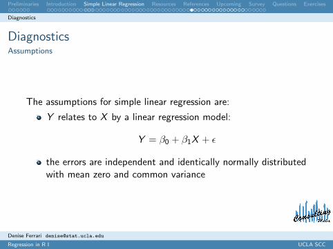
DiagnosticsAssumptions

The assumptions for simple linear regression are:

Y relates to X by a linear regression model:

Y = β0 + β1X + ε

the errors are independent and identically normally distributedwith mean zero and common variance




Diagnostics

DiagnosticsWhat can go wrong?

Violations:

In the linear regression model:

− linearity (e.g. quadratic relationship or higher order terms)

In the residual assumptions:

− non-normal distribution− non-constant variances− dependence− outliers

Checks:

⇒ look at plot of residuals vs. X

⇒ look at plot of residuals vs. fitted values

⇒ look at residuals Q-Q norm plot




Diagnostics

Validity of the regression model IExample: The Anscombe’s data sets (Taken from Sheather, 2009)

1 # Loading the data:

2 anscombe <- read.table("http://www.stat.tamu.edu/~sheather/book/docs/datasets/anscombe.txt", h=T, sep="" )

3 attach(anscombe)4 # Looking at the data:

5 anscombe

case x1 x2 x3 x4 y1 y2 y3 y4

1 10 10 10 8 8.04 9.14 7.46 6.58

2 8 8 8 8 6.95 8.14 6.77 5.76

...

10 7 7 7 8 4.82 7.26 6.42 7.91

11 5 5 5 8 5.68 4.74 5.73 6.89




Diagnostics

Validity of the regression model IIExample: The Anscombe’s data sets (Taken from Sheather, 2009)

1 # Fitting the regressions

2 a1.lm <- lm(y1~x1 , data=anscombe)3 a2.lm <- lm(y2~x2 , data=anscombe)4 a3.lm <- lm(y3~x3 , data=anscombe)5 a4.lm <- lm(y4~x4 , data=anscombe)6

7 #Plotting

8 # For the first data set

9 plot(y1~x1 , data=anscombe)10 abline(a1.lm , col=2)




Diagnostics

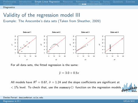
Validity of the regression model IIIExample: The Anscombe’s data sets (Taken from Sheather, 2009)

5 10 15 20

46

810

1214

Data set 1

x1

y1

5 10 15 20

46

810

1214

Data set 2

x2

y2

5 10 15 20

46

810

1214

Data set 3

x3

y3

5 10 15 20

46

810

1214

Data set 4

x4

y4

For all data sets, the fitted regression is the same:

y = 3.0 + 0.5x

All models have R2 = 0.67, σ = 1.24 and the slope coefficients are significant at

< 1% level. To check that, use the summary() function on the regression models.




Diagnostics

Residual Plots IChecking assumptions graphically

Residuals vs. X


2 plot(resid(a1.lm)~x1)

5 10 15 20

-4-2

02

4

Data set 1

x1

Residuals

5 10 15 20

-4-2

02

4

Data set 2

x2

Residuals

5 10 15 20

-4-2

02

4

Data set 3

x3

Residuals

5 10 15 20

-4-2

02

4

Data set 4

x4

Residuals




Diagnostics

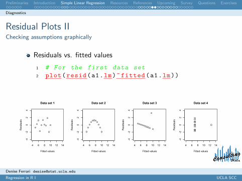
Residual Plots IIChecking assumptions graphically

Residuals vs. fitted values


2 plot(resid(a1.lm)~fitted(a1.lm))

4 6 8 10 12 14

-4-2

02

4

Data set 1

Fitted values

Residuals

4 6 8 10 12 14

-4-2

02

4

Data set 2

Fitted values

Residuals

4 6 8 10 12 14

-4-2

02

4

Data set 3

Fitted values

Residuals

4 6 8 10 12 14

-4-2

02

4

Data set 4

Fitted values

Residuals




Diagnostics

Leverage (or influential) points and outliers I

Leverage points

Leverage points are those which have great influence on the fittedmodel, that is, those whose x-value is distant from the otherx-values.

Bad leverage point: if it is also an outlier, that is, the y -valuedoes not follow the pattern set by the other data points.

Good leverage point: if it is not an outlier.




Diagnostics

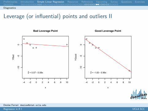
Leverage (or influential) points and outliers II

-4 -2 0 2 4 6 8 10

-10

-50

Bad Leverage Point

x

YBad

y = 0.07 - 0.08x

-4 -2 0 2 4 6 8 10-10

-50

Good Leverage Point

x

YGood

y = -1.83 - 0.96x




Diagnostics

Standardized residuals I

Standardized residuals are obtained by dividing each residual by anestimate of its standard deviation:

ri =ei

σ(ei )

To obtain the standardized residuals in R, use the commandrstandard() on the regression model.

Leverage Points

Good leverage points have their standardized residuals withinthe interval [−2, 2]

Outliers are leverage points whose standardized residuals falloutside the interval [−2, 2]




Diagnostics

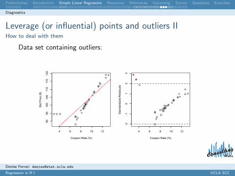
Leverage (or influential) points and outliers IHow to deal with them

Remove invalid data points

⇒ if they look unusual or are different from the rest of the data

Fit a different regression model⇒ if the model is not valid for the data

− higher-order terms− transformation




Diagnostics

Leverage (or influential) points and outliers IIHow to deal with them

Data set containing outliers:

4 6 8 10 12

9095

100

105

110

115

120

Coupon Rate (%)

Bid

Pric

e ($

)

4 6 8 10 12

-2-1

01

23

Coupon Rate (%)

Sta

ndar

dize

d R

esid

uals




Diagnostics

Leverage (or influential) points and outliers IIIHow to deal with them

After their removal:

4 6 8 10 12

9095

100

105

110

115

120

Coupon Rate (%)

Bid

Pric

e ($

)

4 6 8 10 12

-3-2

-10

12

Coupon Rate (%)

Sta

ndar

dize

d R

esid

uals




Diagnostics

Normality and constant variance of errors

Normality and Constant Variance Assumptions

These assumptions are necessary for inference:

hypothesis testing

confidence intervals

prediction intervals

⇒ Check the Normal Q-Q plot of the standardized residuals.

⇒ Check the Standardized Residuals vs. X plot.

Note

When these assumptions do not hold, we can try to correct theproblem using data transformations.




Diagnostics

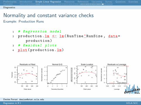
Normality and constant variance checksExample: Production Runs

1 # Regression model

2 production.lm <- lm(RunTime~RunSize , data=production)

3 # Residual plots

4 plot(production.lm)

180 200 220 240

-30

-100

1030

Fitted values

Residuals

Residuals vs Fitted9

810

-2 -1 0 1 2

-10

12

Theoretical Quantiles

Sta

ndar

dize

d re

sidu

als

Normal Q-Q9

810

180 200 220 240

0.0

0.4

0.8

1.2

Fitted values

Standardized residuals

Scale-Location98

10

0.00 0.05 0.10 0.15

-2-1

01

2

Leverage

Sta

ndar

dize

d re

sidu

als

Cook's distance0.5

0.5Residuals vs Leverage

9

1710




Transformations

When to use transformations?

Transformations can be used to correct for:

non-constant variance

non-linearity

non-normality

The most common transformations are:

Square root

Log

Power transformation




Transformations

Example of correction: non-constant variance IExample: Cleaning Data (Taken from Sheather, 2009)

Variables:

Rooms (Y ): number of rooms cleanedCrews (X ): number crews

We want to be able to model the relationship between the numberof rooms cleaned and the number of crews.

1 # Load the data

2 cleaning <- read.table("http://www.stat.tamu.edu/~sheather/book/docs/datasets/cleaning.txt", h=T, sep="")

3 attach(cleaning)




Transformations

Example of correction: non-constant variance IIExample: Cleaning Data (Taken from Sheather, 2009)

1 # Regression model

2 cleaning.lm <- lm(Rooms~Crews , data=cleaning)

3 # Plotting data and

regression line

4 plot(Rooms~Crews)5 abline(cleaning.lm, col=2)

2 4 6 8 10 12 14 16

1020

3040

5060

7080

Crews

Rooms




Transformations

Example of correction: non-constant variance IIIExample: Cleaning Data (Taken from Sheather, 2009)

1 # Diagnostic plots

2 plot(cleaning.lm)

10 20 30 40 50 60

-20

-10

010

20

Fitted values

Residuals


5

-2 -1 0 1 2

-2-1

01

2


Sta

ndar

dize

d re

sidu

als

Normal Q-Q46

5

31

10 20 30 40 50 60

0.0

0.5

1.0

1.5

Fitted valuesStandardized residuals

Scale-Location46531

0.00 0.02 0.04 0.06

-2-1

01

2

Leverage

Sta

ndar

dize

d re

sidu

als

Residuals vs Leverage46

54




Transformations

Example of correction: non-constant variance IVExample: Cleaning Data (Taken from Sheather, 2009)

1 # Applying square root

transformation (counts)

2 sqrtRooms <- sqrt(Rooms)3 sqrtCrews <- sqrt(Crews)4 # Regression model on the

transformed data

5 sqrt.lm <- lm(sqrtRooms~sqrtCrews)

6 # Plotting data and

regression line

7 plot(sqrtRooms~sqrtCrews)8 abline(sqrt.lm, col=2)

1.5 2.0 2.5 3.0 3.5 4.0

34

56

78

9

Cleaning Data Transformed

sqrtCrews

sqrtRooms




Transformations

Example of correction: non-constant variance VExample: Cleaning Data (Taken from Sheather, 2009)

1 # Diagnostic plots

2 plot(sqrt.lm)

3 4 5 6 7 8

-1.0

0.00.51.0

Fitted values

Residuals


5

46

-2 -1 0 1 2

-2-1

01

2


Sta

ndar

dize

d re

sidu

als

Normal Q-Q31

5

46

3 4 5 6 7 80.0

0.4

0.8

1.2

Fitted values

Standardized residuals

Scale-Location31 546

0.00 0.02 0.04 0.06

-2-1

01

2

Leverage

Sta

ndar

dize

d re

sidu

als

Residuals vs Leverage

5

46

4

