introduction to regression models for panel data analysis ... · • panel analysis may be...

Introduction to Regression Models for Panel Data Analysis

Indiana University Workshop in Methods

February 13, 2015

Professor Patricia A. McManus

Panel Data Analysis February 2015

What are Panel Data? Panel data are a type of longitudinal data, or data collected at different points in time. Three main types of longitudinal data:

• Time series data. Many observations (large t) on as few as one unit (small

N). Examples: stock price trends, aggregate national statistics. • Pooled cross sections. Two or more independent samples of many units

(large N) drawn from the same population at different time periods: o General Social Surveys o US Decennial Census extracts o Current Population Surveys*

• Panel data. Two or more observations (small t) on many units (large N).

o Panel surveys of households and individuals (PSID, NLSY, ANES) o Data on organizations and firms at different time points o Aggregated regional data over time

• This workshop is a basic introduction to the analysis of panel data. In

particular, I will cover the linear error components model.

WIM Panel Data Analysis October 2015| Page 1

Why Analyze Panel Data? • We are interested in describing change over time

o social change, e.g. changing attitudes, behaviors, social relationships o individual growth or development, e.g. life-course studies, child

development, career trajectories, school achievement o occurrence (or non-occurrence) of events

• We want superior estimates trends in social phenomena

o Panel models can be used to inform policy – e.g. health, obesity o Multiple observations on each unit can provide superior estimates as

compared to cross-sectional models of association • We want to estimate causal models

o Policy evaluation o Estimation of treatment effects


What kind of data are required for panel analysis? • Basic panel methods require at least two “waves” of measurement.

Consider student GPAs and job hours during two semesters of college.

• One way to organize the panel data is to create a single record for each

combination of unit and time period: StudentID Semester Female HSGPA GPA JobHrs 17 5 0 2.8 3.0 0 17 6 0 2.8 2.1 20 23 5 1 2.5 2.2 10 23 6 1 2.5 2.5 10

• Notice that the data include: o A time-invariant unique identifier for each unit (StudentID) o A time-varying outcome (GPA) o An indicator for time (Semester).

• Panel datasets can include other time-varying or time-invariant variables


• An alternative way to structure the data is to keep all the measures related to each student in a single record. This is sometimes called “wide” format.

StudentID Female HSGPA GPA5 JobHrs5 GPA6 JobHrs6 17 0 2.8 3.0 0 2.1 20 23 1 2.5 2.2 10 2.5 10

o Why are there two variables for GPA and JobHrs ?

o Why is there only one variable for gender and high school GPA?

o Where is the indicator for time?


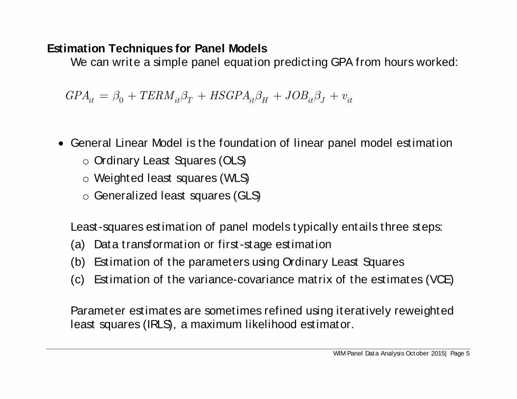
Estimation Techniques for Panel Models We can write a simple panel equation predicting GPA from hours worked:

0it it T it H it J itGPA TERM HSGPA JOB vb b b b= + + + +

• General Linear Model is the foundation of linear panel model estimation

o Ordinary Least Squares (OLS) o Weighted least squares (WLS) o Generalized least squares (GLS)

Least-squares estimation of panel models typically entails three steps: (a) Data transformation or first-stage estimation (b) Estimation of the parameters using Ordinary Least Squares (c) Estimation of the variance-covariance matrix of the estimates (VCE) Parameter estimates are sometimes refined using iteratively reweighted least squares (IRLS), a maximum likelihood estimator.


Basic Questions for the Panel Analyst What’s the story you want to tell? • Is this a descriptive analysis? Less worry, fewer controls are usually better. • Is this an attempt at causal analysis using observational data? Careful

specification AND theory are essential.

How does time matter? • Some analyses, e.g. difference-in-difference analysis associates time with

an event (before and after) • Some analyses may be interested in growth trajectories. • Panel analysis may be appropriate even if time is irrelevant. Panel models

using cross-sectional data collected at fixed periods of time generally use dummy variables for each time period in a two-way specification with fixed-effects for time.

Are the data up to the demands of the analysis? • Panel analysis is data-intensive. Two waves are a bare minimum • Can you perform the necessary specification tests? • How will you address panel attrition?


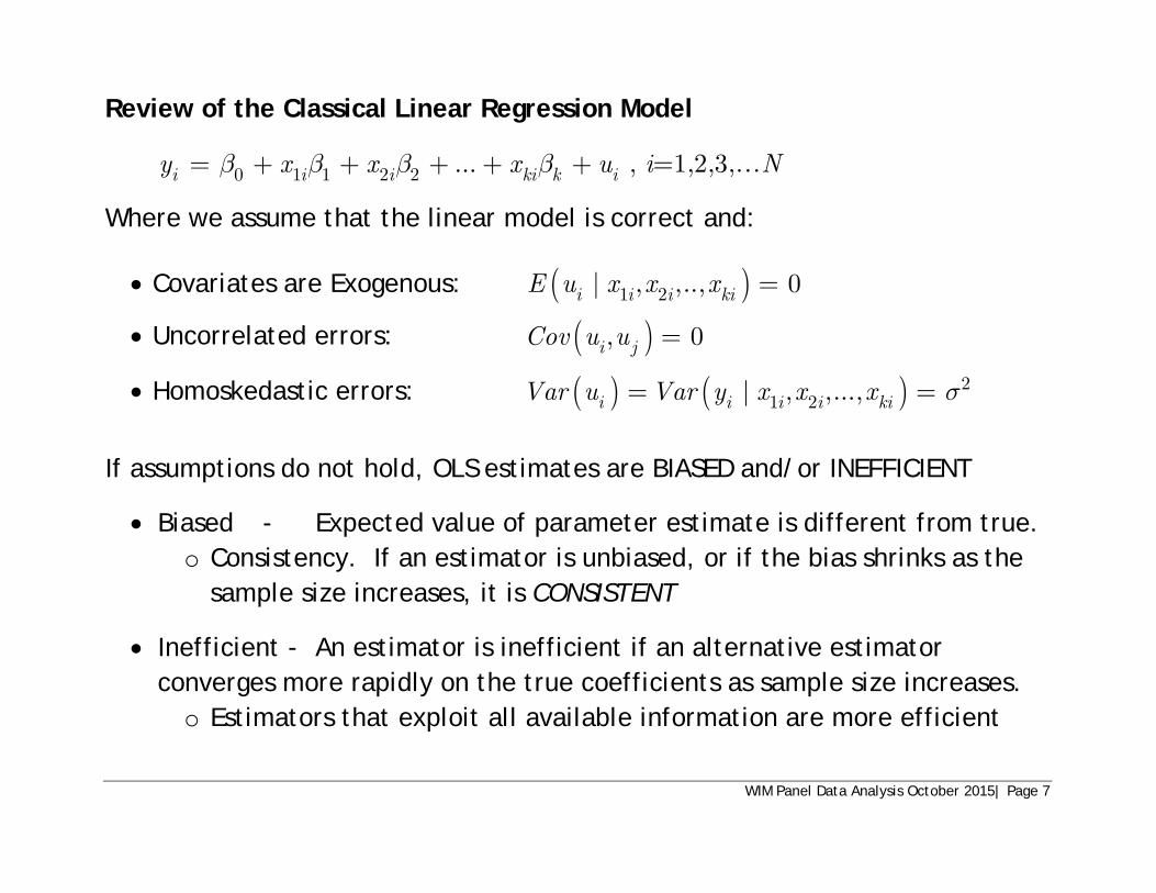
Review of the Classical Linear Regression Model

0 1 1 2 2 ...i i i ki k iy x x x ub b b b= + + + + + , i=1,2,3,…N

Where we assume that the linear model is correct and: • Covariates are Exogenous: ( )1 2| , ,.., 0i i i kiE u x x x =

• Uncorrelated errors: ( ), 0i jCov u u =

• Homoskedastic errors: ( ) ( ) 21 2| , ,...,i i i i kiVar u Var y x x x s= =

If assumptions do not hold, OLS estimates are BIASED and/or INEFFICIENT

• Biased - Expected value of parameter estimate is different from true. o Consistency. If an estimator is unbiased, or if the bias shrinks as the

sample size increases, it is CONSISTENT

• Inefficient - An estimator is inefficient if an alternative estimator converges more rapidly on the true coefficients as sample size increases. o Estimators that exploit all available information are more efficient


OLS Bias Due to Endogeneity • Omitted Variable Bias

o Intervening variables, selectivity

• Measurement Error in the Covariates

• Simultaneity Bias o Feedback loops o Omitted variables

Conventional regression-based strategies to address endogeneity bias • Instrumental Variables estimation • Structural Equations Models • Propensity score estimation • Fixed effects panel models


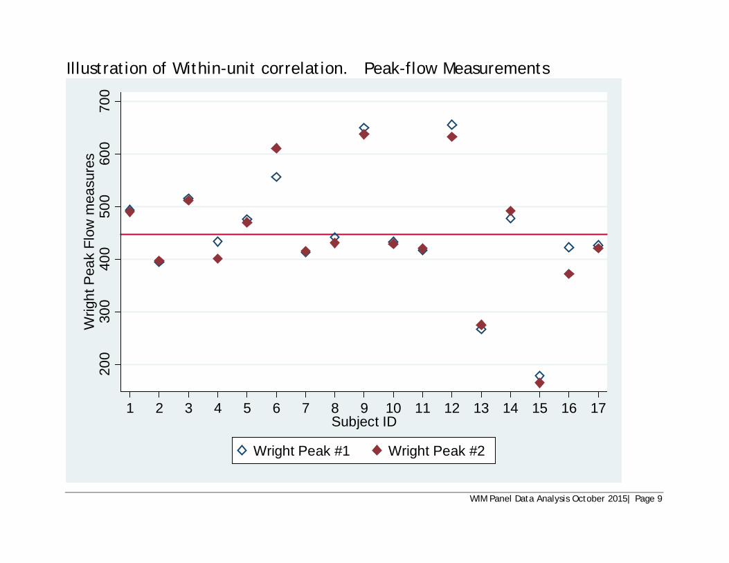
Illustration of Within-unit correlation. Peak-flow Measurements

200

300

400

500

600

700

Wrig

ht P

eak

Flow

mea

sure

s

1 2 3 4 5 6 7 8 9 10 11 12 13 14 15 16 17Subject ID

Wright Peak #1 Wright Peak #2


OLS Inefficiency due to Correlated Errors

Many data structures are susceptible to error correlation:

• Hierarchical data sample multiple individuals from each unit, e.g. household members, employees in firms, multiple pupils from each school.

• Multistage probability samples often incorporate cluster-based sampling designs with errors that may be correlated within clusters.

• Repeated observations data often show within-unit error correlation.

• Time series data often have errors that are serially correlated, that is, correlated over time.

• Panel data have errors that can be correlated within unit (e.g. individuals), within period.

Conventional regression-based strategies to address correlated errors • Cluster-consistent covariance matrix estimator to adjust standard errors.

• Generalized Least Squares instead of OLS to exploit correlation structure.

• Generalized Estimation Equations (GEE)

• Mixed Effects Estimators for multilevel models


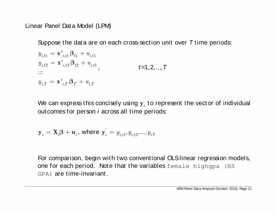
Linear Panel Data Model (LPM) Suppose the data are on each cross-section unit over T time periods:

, 1 , 1 1 , 1

, 2 , 2 2 , 1

, , ,

'

'

:::

'

i t i t t i t

i t i t t i t

i T i T T i T

y u

y u

y u

= += +

= +

xx

x

bb

b

, t=1,2,…,T

We can express this concisely using iy to represent the vector of individual outcomes for person i across all time periods:

i i i= +y X ub , where ', 1 , 2, ,...,i i t i t iTy y y=y

For comparison, begin with two conventional OLS linear regression models, one for each period. Note that the variables female highgpa (HS GPA) are time-invariant.


OLS Results for each term: Term 5 GPA Term 6 GPA Estimate SE t-stat Estimate SE t-stat Intercept 3.02 0.17 17.8 3.02 0.17 18.3 jobhrs -0.182 0.05 -4.0 -0.174 0.05 -3.6 female 0.108 0.04 2.5 0.145 0.05 3.2 highgpa -0.004 0.04 -0.1 0.003 0.04 0.1 Pooled OLS Results for both terms: Term 5&6 GPA Term 5&6 GPA (Clustered SE) Estimate SE t-stat Estimate SE t-stat Intercept 2.97 0.17 25.1 2.97 0.17 17.2 jobhrs -0.178 0.05 -5.4 -0.178 0.05 -5.8 female 0.125 0.04 4.1 0.125 0.04 3.0 highgpa -0.0001 0.03 -0.01 0.0001 0.03 -0.0004 term6 0.095 0.016 6.1 0.095 0.016 6.1


Linear Unobserved Effects Panel Data Model • Motivation: Unobserved heterogeneity

Suppose we have a model with an unobserved, time-constant variable c:

0 1 1 2 2 ... k ky x x x c ub b b b= + + + + + +

Where u is uncorrelated with all explanatory variables in x. Because c is unobserved it is absorbed into the error term, so we can write the model as follows:

0 1 1 2 2 ... k ky x x x v

v c u

b b b b= + + + + += +

The error term v consists of two components, an “idiosyncratic” component u and an “unobserved heterogeneity” component c .


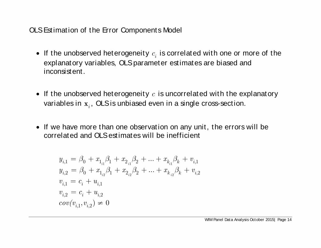
OLS Estimation of the Error Components Model

• If the unobserved heterogeneity ic is correlated with one or more of the explanatory variables, OLS parameter estimates are biased and inconsistent.

• If the unobserved heterogeneity c is uncorrelated with the explanatory variables in ix , OLS is unbiased even in a single cross-section.

• If we have more than one observation on any unit, the errors will be correlated and OLS estimates will be inefficient

1 1 1

2 2 2

,1 0 1 1 2 2 ,1

,2 0 1 1 2 2 ,2

,1 ,1

,2 ,2

,1 ,2

...

...

, ) 0

i i i

i i i

i k k i

i k k i

i i i

i i i

i i

y x x x v

y x x x v

v c u

v c u

cov(v v

b b b bb b b b

= + + + + +

= + + + + +

= += +

¹


• Unobserved Heterogeneity in Panel Data Suppose the data are on each cross-section unit over T time periods. This is an unobserved effects model (UEM), also called the error components model. We can write the model for each time period:

1 1

2 2

i i i i

i i i i

iT iT i iT

y c u

y c u

y c u

= + += + +

= + +

1

2

xx

x

bb

b

,

Where there are T observations on outcome y for person i,

itx is a vector of explanatory variables measured at time t,

ic is unobserved in all periods but constant over time

itu is a time-varying idiosyncratic error

Define it i itv c u= + as the composite error.


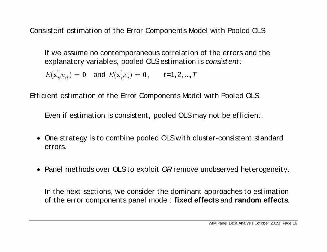
Consistent estimation of the Error Components Model with Pooled OLS If we assume no contemporaneous correlation of the errors and the explanatory variables, pooled OLS estimation is consistent:

'( )it itE u =x 0 and '( )it iE c =x 0, t=1,2,…,T

Efficient estimation of the Error Components Model with Pooled OLS

Even if estimation is consistent, pooled OLS may not be efficient.

• One strategy is to combine pooled OLS with cluster-consistent standard errors.

• Panel methods over OLS to exploit OR remove unobserved heterogeneity. In the next sections, we consider the dominant approaches to estimation of the error components panel model: fixed effects and random effects.


Just a few panel data examples:

• Wage penalty for motherhood

• Men’s wage premium for heterosexual marriage

• Effect of regulation of nursing pay on hospital quality

• Effect of Incarceration on wages and income inequality

• Effect of parental divorce on mental health over life-course

• Determinants of Death Penalty in US states

• Effect of Democracy on Human Capital and Economic Growth


Fixed Effects Methods for Panel Data

Suppose the unobserved effect ic is correlated with the covariates.

Example: Motherhood wage penalty

• We observe that mothers earn less than other women, cet par. ˆ 0.08

OLSKIDSb = . in a log wage model suggests that each additional

child reduces mothers’ hourly wages by about 8% But if women who are less oriented towards work are also more likely to have more children, omitting “work orientations” from the model will bias the coefficient on children.

• Fixed-effects methods transform the model to remove ic

ˆ 0.03FEKIDSb = . FE estimates a persistent but much smaller penalty.


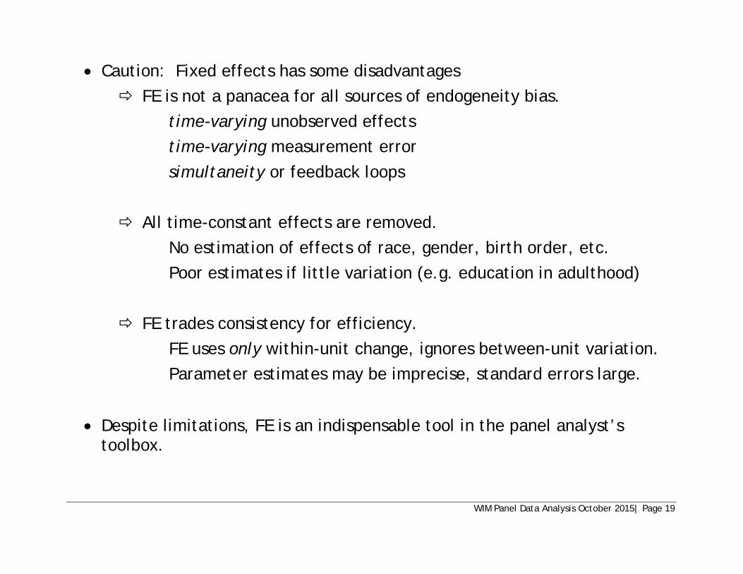
• Caution: Fixed effects has some disadvantages FE is not a panacea for all sources of endogeneity bias.

time-varying unobserved effects time-varying measurement error simultaneity or feedback loops

All time-constant effects are removed. No estimation of effects of race, gender, birth order, etc. Poor estimates if little variation (e.g. education in adulthood)

FE trades consistency for efficiency.

FE uses only within-unit change, ignores between-unit variation. Parameter estimates may be imprecise, standard errors large.

• Despite limitations, FE is an indispensable tool in the panel analyst’s toolbox.


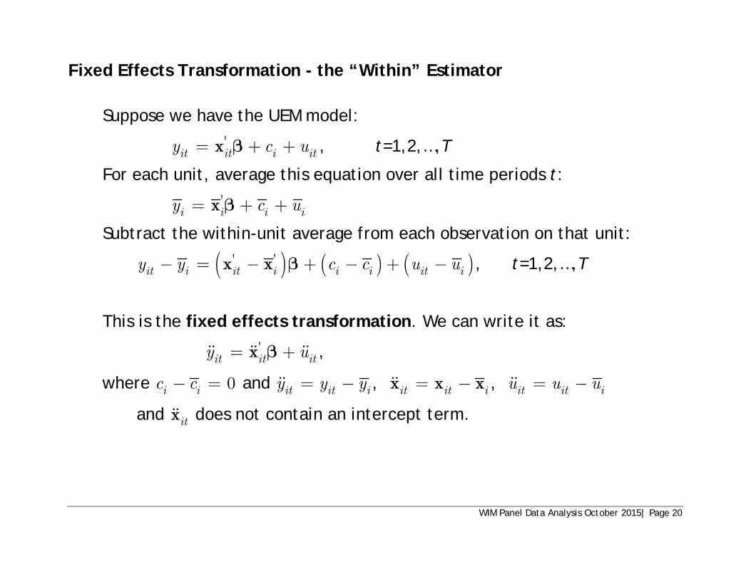
Fixed Effects Transformation - the “Within” Estimator Suppose we have the UEM model:

'it it i ity c u= + +x b , t=1,2,…,T

For each unit, average this equation over all time periods t:

'i i i iy c u= + +x b

Subtract the within-unit average from each observation on that unit:

( ) ( ) ( )' 'it i it i i i it iy y c c u u. = . + . + .x x b , t=1,2,…,T

This is the fixed effects transformation. We can write it as:

'it it ity u= +x b ,

where 0i ic c. = and it it iy y y= . , it it i= .x x x , it it iu u u= .

and itx does not contain an intercept term.


The fixed-effects estimator, also called the within estimator, applies pooled OLS to the transformed equation:

1 1

' ' ' '

1 1 1 1 1 1

ˆN N N T N T

FE i i i i it it it iti i i t i t

y

. .

= = = = = =

æ ö æ ö æ ö æ ö÷ ÷ ÷ ÷ç ç ç ç÷ ÷ ÷ ÷ç ç ç ç= =÷ ÷ ÷ ÷ç ç ç ç÷ ÷ ÷ ÷ç ç ç ç÷ ÷ ÷ ÷è ø è ø è ø è øå å åå ååX X X y x x xb

Recall the student GPA Data: StudentID Semester Female HSGPA GPA JobHrs 17 5 0 2.8 3.0 0 17 6 0 2.8 2.1 20 23 5 1 2.5 2.2 10 23 6 1 2.5 2.5 10 After applying the fixed-effects transform, the demeaned (mean-centered) data: StudentID Semester CFemale CHSGPA CGPA CJobHrs 17 -.5 0 0 .45 -10 17 .5 0 0 -.45 10 23 -.5 0 0 -.15 0 23 .5 0 0 .15 0


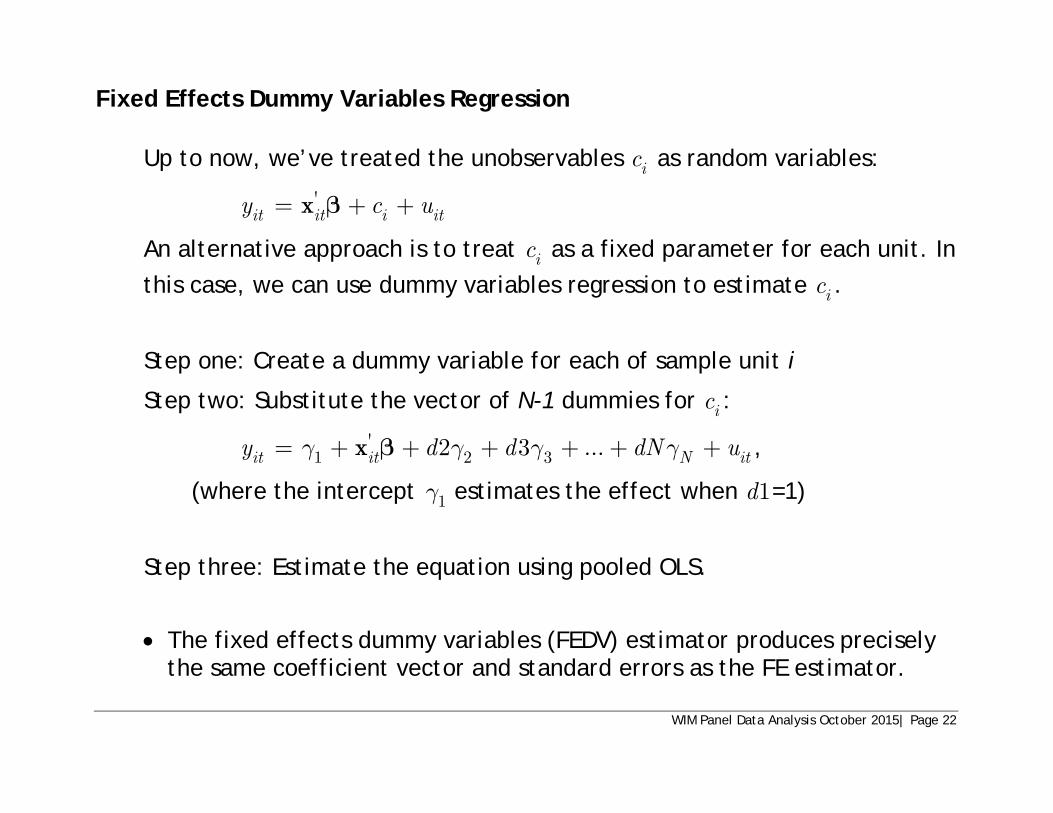
Fixed Effects Dummy Variables Regression

Up to now, we’ve treated the unobservables ic as random variables:

'it it i ity c u= + +x b

An alternative approach is to treat ic as a fixed parameter for each unit. In this case, we can use dummy variables regression to estimate ic .

Step one: Create a dummy variable for each of sample unit i

Step two: Substitute the vector of N-1 dummies for ic :

'1 2 32 3 ...it it N ity d d dN ug g g g= + + + + + +x b ,

(where the intercept 1g estimates the effect when 1d =1)

Step three: Estimate the equation using pooled OLS.

• The fixed effects dummy variables (FEDV) estimator produces precisely the same coefficient vector and standard errors as the FE estimator.


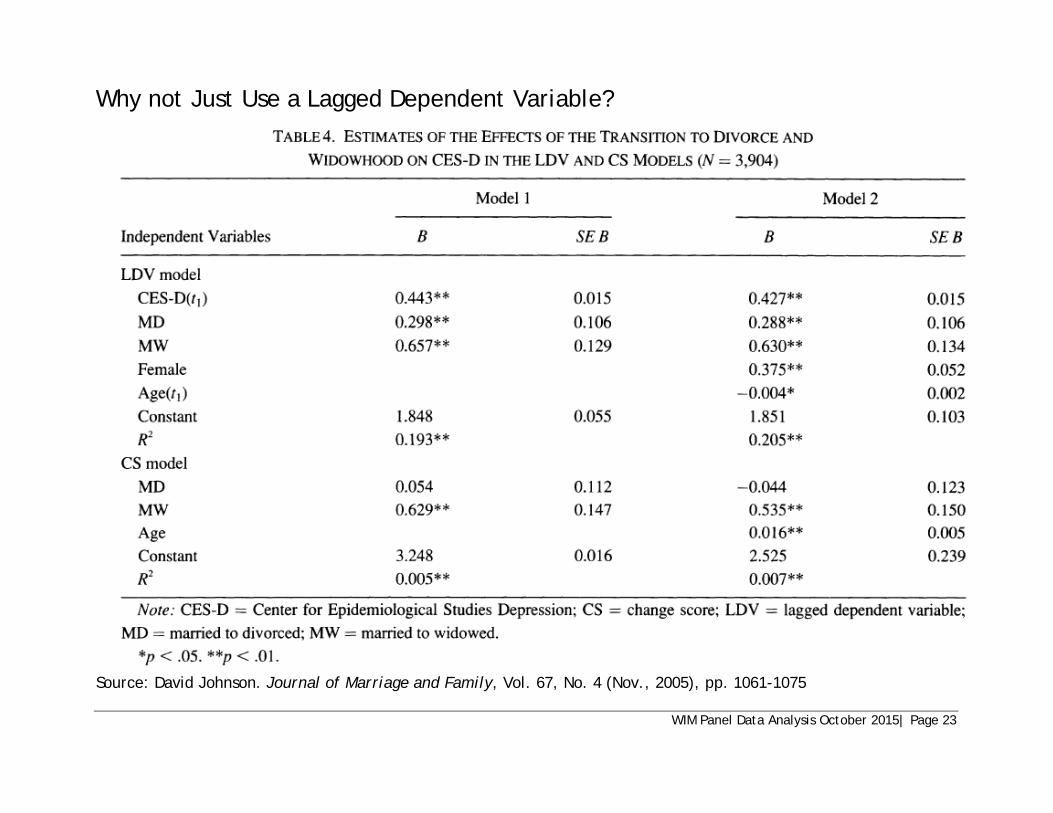
Why not Just Use a Lagged Dependent Variable?

Source: David Johnson. Journal of Marriage and Family, Vol. 67, No. 4 (Nov., 2005), pp. 1061-1075


Random Effects Methods If we can assume that the unobserved heterogeneity will not bias the estimates:

• Fixed effects methods are inefficient. They throw away information.

• Pooled OLS is inefficient because it does not exploit the autocorrelation in the composite error term.

• Random effects methods use feasible GLS estimation (RE FGLS) to exploit within-cluster correlation

• Random effects estimation is more efficient than FE or OLS

• The “random effects assumption” of no bias due to ic is more stringent

1( | ,..., ) ( ) 0i i iT iE c E c= =x x


A Conventional FGLS Random Effects Estimator Assume the errors are correlated within each unit Assume the errors are uncorrelated across units Assume the variance in the composite errors is equal to the sum of the variances in the unobserved effect ic and the idiosyncratic error iu :

2 2 2v u cs s s= +

RE strategy: If 2 2 2v u cs s s= + , find estimators such that 2 2 2ˆ ˆ ˆv u cs s s= +


Practical Feature of Random Effects Estimation

• Recall that the fixed effects “within” estimator essentially transforms the data by centering each variable on the unit-specific mean. OLS is then performed on the “fully demeaned” transformed data.

• The random effects estimator essentially transforms the data by “partially demeaning” each variable. Instead of subtracting the entire unit-specific mean, only part of the mean is subtracted. The demeaning factor l is between 0 and 1, with the specific value based on the variance components estimation.


RE Results compared to pooled OLS Results for two terms: RE Term 5&6 GPA OLS Term 5&6 GPA Estimate SE z-stat Estimate SE t-stat Intercept 2.81 0.16 18.0 2.97 0.17 17.2 jobhrs -0.108 0.02 -4.8 -0.178 0.05 -5.8 female 0.126 0.04 3.0 0.125 0.04 3.0 highgpa -0.001 0.03 -0.04 0.0001 0.03 -0.0004 term6 0.096 0.015 5.6 0.095 0.016 6.1 RE Results for six terms: Terms 1-6 GPA (FE, N=400) Estimate SE Intercept 2.41 0.10 23.5 jobhrs -0.129 0.02 -7.0 female 0.086 0.03 2.8 highgpa -0.030 0.02 1.2 term 0.088 0.006 13.6


Random Effects or Fixed Effects - How to decide? Hausman test for the Exogeneity of the Unobserved Error Component If the unobserved effects are exogenous, the FE and RE are asymptotically equivalent. This suggests the null hypothesis for the Hausman test:

0ˆ ˆ: RE FEH =b b ,

where ˆREb and ˆFEb are coefficient vectors for the time-varying explanatory variables, excluding the time variables. If the null hypothesis is rejected, we conclude that RE is inconsistent, and the FE model is preferred. If the null hypothesis cannot be rejected, random effects is preferred because it is a more efficient estimator.


Conventional Hausman Test in Stata: . xtreg gpa job sex highgpa,fe . estimates store fe . xtreg gpa job sex highgpa,re . estimates store re . hausman fe re ---- Coefficients ---- | (b) (B) (b-B) sqrt(diag(V_b-V_B)) | fe re Difference S.E. -------------+--------------------------------------------------------------- job | -.0748115 -.1232374 .048426 .0088051 ----------------------------------------------------------------------------- b = consistent under Ho and Ha; obtained from xtreg B = inconsistent under Ha, efficient under Ho; obtained from xtreg Test: Ho: difference in coefficients not systematic chi2(1) = (b-B)'[(V_b-V_B)^(-1)](b-B) = 30.25 Prob>chi2 = 0.0000

• We reject the null and conclude the fixed effects estimator is appropriate.


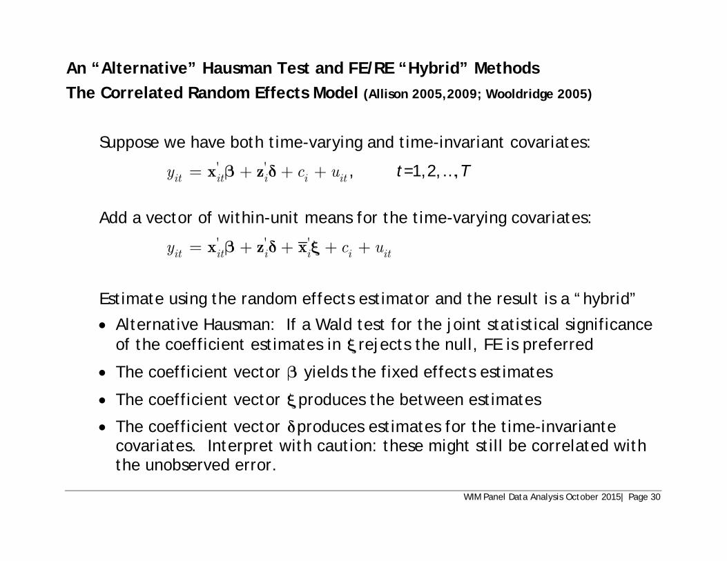
An “Alternative” Hausman Test and FE/RE “Hybrid” Methods The Correlated Random Effects Model (Allison 2005,2009; Wooldridge 2005)

Suppose we have both time-varying and time-invariant covariates:

' 'it it i i ity c u= + + +x zb d , t=1,2,…,T

Add a vector of within-unit means for the time-varying covariates:

' ' 'it it i i i ity c u= + + + +x z xb d y

Estimate using the random effects estimator and the result is a “hybrid”

• Alternative Hausman: If a Wald test for the joint statistical significance of the coefficient estimates in y rejects the null, FE is preferred

• The coefficient vector b yields the fixed effects estimates

• The coefficient vector yproduces the between estimates

• The coefficient vector dproduces estimates for the time-invariante covariates. Interpret with caution: these might still be correlated with the unobserved error.


Interpretation of Results from the Error Components Model Since the UEM model is derived as a levels model, coefficients can be interpreted much the same as interpretations of a conventional OLS model, but there are nuances: For example, suppose we estimate the relationship between marriage and men’s wages, ˆ 0.05MARRIEDb in every model.

• Pooled OLS cross-section coefficients contain information about average differences between units.

[ | ]it it it iE y c= +x x b

This is a population-averaged effect. On average, married men earn 5% more than men who are not married. This says nothing about the causal effect of marriage on men’s earnings.


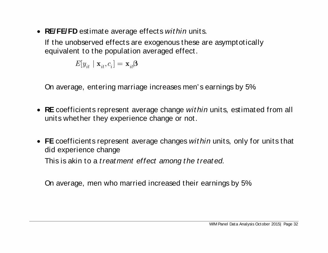
• RE/FE/FD estimate average effects within units. If the unobserved effects are exogenous these are asymptotically equivalent to the population averaged effect.

[ | , ]it it i itE y c =x x b

On average, entering marriage increases men’s earnings by 5%.

• RE coefficients represent average change within units, estimated from all units whether they experience change or not.

• FE coefficients represent average changes within units, only for units that did experience change This is akin to a treatment effect among the treated. On average, men who married increased their earnings by 5%.


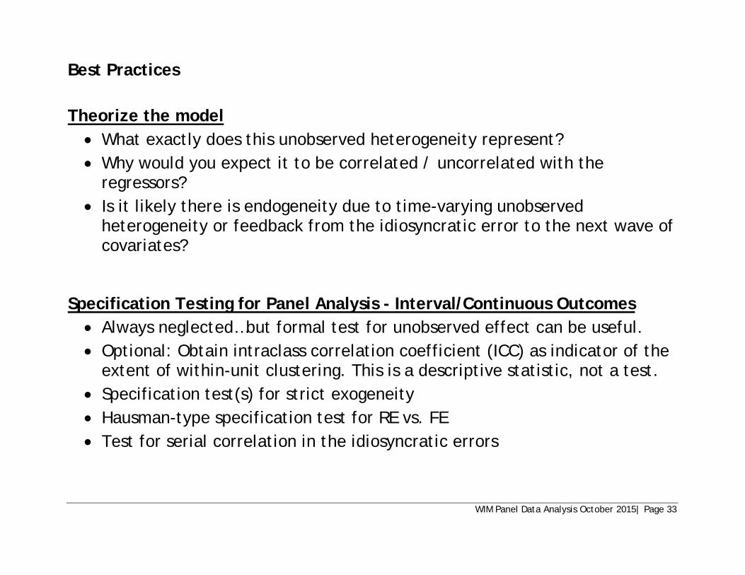
Best Practices

Theorize the model • What exactly does this unobserved heterogeneity represent? • Why would you expect it to be correlated / uncorrelated with the

regressors? • Is it likely there is endogeneity due to time-varying unobserved

heterogeneity or feedback from the idiosyncratic error to the next wave of covariates?

Specification Testing for Panel Analysis - Interval/Continuous Outcomes • Always neglected…but formal test for unobserved effect can be useful. • Optional: Obtain intraclass correlation coefficient (ICC) as indicator of the

extent of within-unit clustering. This is a descriptive statistic, not a test. • Specification test(s) for strict exogeneity • Hausman-type specification test for RE vs. FE • Test for serial correlation in the idiosyncratic errors


Extensions FE Models with Time-Invariant Predictors

• Interactions between time and covariate Panel Models for Categorical Outcomes • Fixed effects logit and random effects logit for binary outcomes • Fixed and random effects Poisson models can be used for count outcomes. • Population averaged models can be estimated using General Estimation

Equations (GEE).

Dynamic panel models i.e. lagged dependent variable as a covariate:

0 , 1it i t GPA it T it H it J itGPA GPA TERM HSGPA JOB vb b b b b.= + + + + +

• GLM models for instrumental variables (IV) estimation

• Generalized Method of Moments (GMM) is used for some dynamic panel models because it allows a flexible specification of the instruments


introduction to regression models for panel data analysis ... · • panel analysis may be...

Documents