introduction to relativity and geometric analysis...it begins with special relativity, then moves to...
TRANSCRIPT
Introduction to Relativity
and Geometric Analysis
MTH 6132 Course notes
Autumn 2015
Dr. Shabnam Beheshti and Dr. Juan A. Valiente Kroon
(adapted from notes from Prof. Reza Tavakol)
School of Mathematical Sciences
Queen Mary, University of London
Mile End Road, London E1 4NS
1

2
Contents
1 Introduction 31.1 What is Relativity? . . . . . . . . . . . . . . . . . . . . . . . . . . . . . . . 3
1.1.1 Special Relativity? . . . . . . . . . . . . . . . . . . . . . . . . . . . 31.1.2 General Relativity? . . . . . . . . . . . . . . . . . . . . . . . . . . . 3
1.2 Pre-relativistic Physics . . . . . . . . . . . . . . . . . . . . . . . . . . . . . 41.2.1 Galilean Relativity . . . . . . . . . . . . . . . . . . . . . . . . . . . 41.2.2 Laws of Newton . . . . . . . . . . . . . . . . . . . . . . . . . . . . 41.2.3 Galilean transformations . . . . . . . . . . . . . . . . . . . . . . . . 51.2.4 Galilean transformation formulae for the velocity and acceleration 61.2.5 Invariance of Newton’s laws under Galilean transformations . . . . 61.2.6 Electromagnetism . . . . . . . . . . . . . . . . . . . . . . . . . . . 7
2 Special Relativity 92.1 Einstein’s postulates of Special Relativity . . . . . . . . . . . . . . . . . . 92.2 Spacetime diagrams . . . . . . . . . . . . . . . . . . . . . . . . . . . . . . 92.3 Lorentz transformations (LT) . . . . . . . . . . . . . . . . . . . . . . . . . 132.4 Clocks and rods in relativistic motion . . . . . . . . . . . . . . . . . . . . 14
2.4.1 Time dilation . . . . . . . . . . . . . . . . . . . . . . . . . . . . . . 142.4.2 Length contraction . . . . . . . . . . . . . . . . . . . . . . . . . . . 14
2.5 Paradoxes . . . . . . . . . . . . . . . . . . . . . . . . . . . . . . . . . . . . 152.6 Experimental evidence for Special Relativity . . . . . . . . . . . . . . . . . 152.7 The inverse Lorentz transformation . . . . . . . . . . . . . . . . . . . . . . 162.8 Hyperbolic form of the Lorentz transformations . . . . . . . . . . . . . . . 162.9 Further discussion on the Lorentz Transformations . . . . . . . . . . . . . 21
2.9.1 Transformation formula for the velocity . . . . . . . . . . . . . . . 212.9.2 Transformation formula for the acceleration . . . . . . . . . . . . . 21
2.10 The Minkowski spacetime . . . . . . . . . . . . . . . . . . . . . . . . . . . 222.10.1 Minkowski diagrams . . . . . . . . . . . . . . . . . . . . . . . . . . 252.10.2 A brief discussion of causality . . . . . . . . . . . . . . . . . . . . . 25
2.11 4-vectors in Special Relativity . . . . . . . . . . . . . . . . . . . . . . . . . 262.11.1 Index notation . . . . . . . . . . . . . . . . . . . . . . . . . . . . . 272.11.2 4-vectors . . . . . . . . . . . . . . . . . . . . . . . . . . . . . . . . 28
2.12 Proper time . . . . . . . . . . . . . . . . . . . . . . . . . . . . . . . . . . . 312.13 4-velocity and 4-momentum . . . . . . . . . . . . . . . . . . . . . . . . . . 312.14 Photons . . . . . . . . . . . . . . . . . . . . . . . . . . . . . . . . . . . . . 332.15 Doppler shift . . . . . . . . . . . . . . . . . . . . . . . . . . . . . . . . . . 332.16 Relativistic dynamics . . . . . . . . . . . . . . . . . . . . . . . . . . . . . . 34
2.16.1 Examples of relativistic collisions . . . . . . . . . . . . . . . . . . . 34
3
3 Prelude to General Relativity 373.1 General remarks . . . . . . . . . . . . . . . . . . . . . . . . . . . . . . . . 373.2 The Equivalence Principle . . . . . . . . . . . . . . . . . . . . . . . . . . . 373.3 Summary . . . . . . . . . . . . . . . . . . . . . . . . . . . . . . . . . . . . 38
4 Di↵erential Geometry and tensor calculus 394.1 Manifolds and coordinates . . . . . . . . . . . . . . . . . . . . . . . . . . . 394.2 Transformation of coordinates . . . . . . . . . . . . . . . . . . . . . . . . . 404.3 Contravariant vectors . . . . . . . . . . . . . . . . . . . . . . . . . . . . . 414.4 Covariant and mixed tensors . . . . . . . . . . . . . . . . . . . . . . . . . 414.5 Tensor algebra . . . . . . . . . . . . . . . . . . . . . . . . . . . . . . . . . 44
4.5.1 Addition (linear combination) . . . . . . . . . . . . . . . . . . . . . 444.5.2 Direct product . . . . . . . . . . . . . . . . . . . . . . . . . . . . . 454.5.3 Contraction . . . . . . . . . . . . . . . . . . . . . . . . . . . . . . . 454.5.4 Detection of tensors . . . . . . . . . . . . . . . . . . . . . . . . . . 454.5.5 Symmetric and antisymmetric tensors . . . . . . . . . . . . . . . . 46
4.6 Manifolds with metric . . . . . . . . . . . . . . . . . . . . . . . . . . . . . 474.7 Derivatives and connections . . . . . . . . . . . . . . . . . . . . . . . . . . 504.8 Parallel transport . . . . . . . . . . . . . . . . . . . . . . . . . . . . . . . . 514.9 The Levi-Civita connection . . . . . . . . . . . . . . . . . . . . . . . . . . 53
4.9.1 The Christo↵el symbols of the metric of the Euclidean plane . . . 544.10 Metric geodesics . . . . . . . . . . . . . . . . . . . . . . . . . . . . . . . . 55
4.10.1 An example of the use of the Euler-Lagrange equations . . . . . . 57
5 Curvature 595.1 Intrinsic curvature and the Riemann tensor . . . . . . . . . . . . . . . . . 595.2 Geodesic deviation . . . . . . . . . . . . . . . . . . . . . . . . . . . . . . . 615.3 Symmetries of the curvature tensor . . . . . . . . . . . . . . . . . . . . . . 615.4 Bianchi identities, the Ricci and Einstein tensors . . . . . . . . . . . . . . 62
6 General Relativity 656.1 Towards the Einstein equations . . . . . . . . . . . . . . . . . . . . . . . . 656.2 Principles employed in General Relativity . . . . . . . . . . . . . . . . . . 66
6.2.1 The Einstein equations in vacuum . . . . . . . . . . . . . . . . . . 676.2.2 The (full) Einstein Equations . . . . . . . . . . . . . . . . . . . . . 67
6.3 The Schwarzschild solution . . . . . . . . . . . . . . . . . . . . . . . . . . 686.3.1 Newtonian limit . . . . . . . . . . . . . . . . . . . . . . . . . . . . 69
6.4 Applications and Experimental Tests of GR . . . . . . . . . . . . . . . . . 716.4.1 The photon sphere . . . . . . . . . . . . . . . . . . . . . . . . . . . 726.4.2 Timelike case —an orbiting particle . . . . . . . . . . . . . . . . . 736.4.3 Null geodesics . . . . . . . . . . . . . . . . . . . . . . . . . . . . . . 75
6.5 Gravitational redshift . . . . . . . . . . . . . . . . . . . . . . . . . . . . . 776.6 Black holes . . . . . . . . . . . . . . . . . . . . . . . . . . . . . . . . . . . 78
4
Preface
These are notes for the Relativity course (MTH6132) I am currently lecturing duringthe Autumn 2015/Autumn 2016 terms at the School of Mathematical Sciences of QueenMary, University of London. The material is primarily based on both typeset and hand-written notes I have inherited from Dr. Juan Valiente-Kroon and Professor Reza Tavakol;the primary addition I am making to these notes is the discussion of classical and cur-rent problems from geometric analysis which motivate (or are motivated by) GeneralRelativity.
The present course on Relativity is aimed at mathematics and physics undergraduatesinterested in learning the mathematical foundations of Special and General Relativity. Inparticular, very little physical background is assumed, so a certain amount of time is spentpresenting underlying assumptions and experimental motivation for such a theory. Thelectures also assumes minimal prerequisites on the mathematical side. Necessary ideasfrom di↵erential geometry and tensors are self-contained and references are provided forfurther study. The course is quite an ambitious one, divided approximately into thirds.It begins with Special Relativity, then moves to Di↵erential Geometry and finally itprovides an introduction to General Relativity.
Due to time constraints, there are some clear omissions in the choice of topics. Inparticular, in the chapter on Special Relativity it would be desirable to have a discussionof the Maxwell equations. In the chapter on Di↵erential Geometry, it would be elegant todiscuss the Hamilton-Jacobi Equations as motivation for generalizing curvature. In thechapter on General Relativity, the discussion is restricted to the vacuum field equationswith little mention of the field equations with matter. Also, it would be desirable toinclude positive mass theorems, cosmological models and of course, the most recent andexciting progress on gravitational waves! Thorough mathematical investigation of thesetopics would require at the very least a couple of weeks more. Perhaps a re-orgainsation ofthe topics and thoughtful collaboration could result in a two-semester course in GeometricAnalysis and General Relativity. I do not discard the possibility of carrying out such arevision in future iterations of the course. In the meantime, please know that the currentlecture notes have been adapted to my particular understanding and appreciation of thesubject.
Corrections, omissions and suggestions for improvements with which the readers of thesenotes may favour me will be greatly appreciated.
–S. Beheshti
1

2
Chapter 1
Introduction
1.1 What is Relativity?
The term Relativity encompasses two physical theories proposed by Einstein1. Namely,Special Relativity and General Relativity. However, as we will see, the word relativity isalso used in reference to Galilean Relativity
2. The term Theory of Relativity was firstcoined by Max Planck3 in 1906 to emphasize how a theory devised by Einstein in 1905—what we now call Special Relativity— uses the Principle of Relativity.
1.1.1 Special Relativity?
Special Relativity is the physical theory of the measurement in inertial frames of refer-
ence. It was proposed in 1905 by Albert Einstein in the article On the Electrodynamic of
moving bodies (Zur Elektrodynamik bewegter Korper, Annalen der Physik 17, 891 (1905)).It generalises Galileo’s Principle of Relativity —all motion is relative and that there isno absolute and well-defined state of rest. Special Relativity incorporates the principlethat the speed of light is the same for all inertial observers, regardless the state of motionof the source. The theory is termed special because it only applies to the special caseof inertial reference frames —i.e. frames of reference in uniform relative motion withrespect to each other. Special Relativity predicts the equivalence of matter and energyas expressed by the formula
E = mc2.
Special Relativity is a fundamental tool to describe the interaction between elementaryparticles, and was widely accepted by the Physics community by the 1920’s.
1.1.2 General Relativity?
General Relativity is the geometric theory of gravitation published by Albert Einsteinin 1915 in the article The field equations of Gravitation (Die Feldgleichungen der Grav-
itation, Sitzungsberichte der Preussischen Akademie der Wisenschaften zu Berlin 884).It generalises Special Relativity and Newton’s law of universal gravitation, providing aunified description of gravity as the manifestation of the curvature of spacetime. Thetheory is general because it applies the Principle of Relativity to any frame of reference soas to handle general coordinate transformations. From General Relativity it follows that
1Albert Einstein (1879-1955). Physicist of German origin. Died in the USA.
2Galileo Galilei (584-1642) . Italian physicist, mathematician and astronomer.
3Max Planck (1858-1947). German physicist.
3
Special Relativity still applies locally. The domain of applicability of General Relativityis in Astrophysics and Cosmology. More recently, the Global Positioning System (GPS)requires of General Relativity to function accurately! Contrary to Special Relativity,General Relativity was not widely accepted until the 1960’s.
1.2 Pre-relativistic Physics
1.2.1 Galilean Relativity
In order to study General Relativity one starts discussing Special Relativity. To this end,it is important to briefly look at pre-relativistic Physics to see how Special Relativityarose.
The starting point of Special Relativity is the study of motion. For this one needsthe following ingredients:
• Frames of reference. These consist of an origin in space, 3 orthogonal axes anda clock.
• Events. This notion denotes a single point in space together with a single point intime. Thus, events are characterised by 4 real numbers: an ordered triple (x, y, z)giving the location in space relative to a fixed coordinate system and a real numbergiving the Newtonian time. One denotes the event by E = (t, x, y, z).
There are an infinite number of frames of reference. Motion relative to each framelooks, in principle, di↵erent. Hence, it is natural to ask: is there a subset of these frameswhich are in some sense simple, preferred or natural? The answer to this question is yes.These are the so-called inertial frames. In an inertial frame an isolated, non-rotating,unaccelerated body moves on a straight line and uniformly.
Inertial frames are not unique. There are actually an infinite number of these. Thisraises the question: can one tell in which inertial frame are we in? It turns out thatwithin the framework of Newtonian Mechanics this is not possible. More precisely, onehas the following:
Galilean Principle of Relativity. Laws of mechanics cannot distinguish betweeninertial frames. This implies that there is no absolute rest. In other words, the laws ofMechanics retain the same form in di↵erent inertial frames.
In this sense, Relativity predates Einstein.
1.2.2 Laws of Newton
The three Laws of Newtonian Mechanics4 are:
(1) Any material body continues in its state of rest or uniform motion (in a straightline) unless it is made to change the state by forces acting on it. This principle isequivalent to the statement of existence of inertial frames.
(2) The rate of change of momentum is equal to the force.
(3) Action and reaction are equal and opposite.
4Isaac Newton (1643-1727). English physicist and mathematician.
4
These laws or principles, together with the following fundamental assumptions (someof which are implicitly assumed in Newton’s laws) amount to the Newtonian framework :
(A1) Space and time are continuous —i.e. not discrete. This is necessary to make useof the Calculus.
(A2) There is a universal (absolute) time. Di↵erent observers in di↵erent frames mea-sure the same time. In fact, Newton also regarded space to be absolute as well.However, the absoluteness of space is not necessary for the development of theNewtonian framework, as space intervals turn out to be invariant under Galileantransformations. Historically, Newton demanded this for subjective reasons.
(A3) Mass remains invariant as viewed from di↵erent inertial frames.
(A4) The Geometry of space is Euclidean. For example, the sum of angles in any triangleequals 180 degrees.
(A5) There is no limit to the accuracy with which quantities such as time and space canbe measured.
As it will be seen in the sequel, Assumptions 2 and 3 are relaxed in Special Relativitywhile Assumption 4 is relaxed in General Relativity. Assumption 5 is relaxed in QuantumMechanics —not to be discussed in the course. Presumably Assumption 1 will be relaxedin Quantum Gravity!
1.2.3 Galilean transformations
Galilean transformations tell us how to transform from one inertial frame to another.
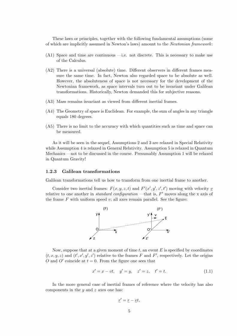
Consider two inertial frames: F (x, y, z, t) and F 0(x0, y0, z0, t0) moving with velocity vrelative to one another in standard configuration —that is, F 0 moves along the x axis ofthe frame F with uniform speed v; all axes remain parallel. See the figure:
�
�
�
��
��
��
�
� ��
�� ���
Now, suppose that at a given moment of time t, an event E is specified by coordinates(t, x, y, z) and (t0, x0, y0, z0) relative to the frames F and F 0, respectively. Let the originsO and O0 coincide at t = 0. From the figure one sees that
x0 = x� vt, y0 = y, z0 = z, t0 = t. (1.1)
In the more general case of inertial frames of reference where the velocity has alsocomponents in the y and z axes one has:
r0 = r � vt,
5
where v = (vx, vy, vz) and r = (x, y, z), r0 = (x0, y0, z0) are the position vectors withrespect to the frames F and F 0, respectively. Notice that in the case of frames of referencein standard configuration one has vy = vz = 0).
Remark. It is customary to call the observer associated to the inertial frame F , Joe,and that of F 0, Moe.
1.2.4 Galilean transformation formulae for the velocity and accelera-tion
To see this, let the position of a particle P be specified by r = r(t) relative to a frameF . The motion relative to F 0 is given by equation (1.1). Di↵erentiating both sides twicewith respect to t (notice that t = t0) gives:
V 0 = V � v, (1.2a)
a0 = a, (1.2b)
where
V =dr
dt, a =
d2r
dt2,
are, respectively, the velocity and acceleration of the particle with respect to the frameF while
V 0 =dr0
dt, a0 =
d2r0
dt2,
are the velocity and acceleration of the particle with respect to F 0.
Remark. Notice that as a consequence of the transformation formula for the acceler-ation (1.2b), the acceleration of the particle as measured by F and F 0 coincide. Thus,although the position and the velocity are di↵erent in each system of reference, both setsof observers agree on the acceleration. This result is some times phrased as: accelerationis Universal.
Example. The following example will be of relevance in the sequel. Consider a cannon-ball moving along the x-axis. If the cannonball has velocity V with respect to the frameF , then the velocity as measured by the frame F 0 (moving with velocity v with respectto F ) is given by V 0 = V � v. In what follows, suppose for simplicity that v > 0. Thenif V > 0 (i.e. the cannonball moves away from the origin of F ) then V 0 = V � v < V—that is, F 0 sees the cannonball moving more slowly. On the other hand if V < 0 (thecannonball goes towards the origin of F ), then |V �v| > v so that F 0 sees the cannonballmoving faster.
1.2.5 Invariance of Newton’s laws under Galilean transformations
Important for the sequel is the notion of invariance. Invariance refers to properties ofa system that remain unchanged under a particular type of transformations. In theprevious section we have already seen that two inertial systems of reference measure thesame acceleration of a moving particle. Thus, acceleration is an invariant under Galileantransformations.
In what follows, we will see that the laws of Mechanics keep the same form as wego from one inertial frame to another —i.e. under Galilean transformations. The First
6
and Third Laws are invariant as the former involves inertial frames and the latter in-volves accelerations which are invariant. It remains to show that the Second Law (thefundamental equation of Newtonian Mechanics)
mdV
dt= ma = f (1.3)
is invariant as we go from one inertial frame to another.
To show the invariance of (1.3) recall that a0 = a and m remains invariant (byassumption) so that one only needs to show that f remains invariant as we go from F toF 0. To do this, recall that generally f takes the form f = f(r, v, t) where usually r andv are the relative distance and the relative velocity between two bodies. One can verifythat the relative distances and velocities remain invariant. That is,
V 02 � V 0
1 = V 2 � V 1, r02 � r01 = r2 � r1.
This implies that f , and hence the Second Law remains invariant under changes in theinertial frames.
This discussion amounts to a form of self-consistency, in the sense that Physics, whenconfined to Newtonian Mechanics, satisfies the Galilean Principle of Relativity.
1.2.6 Electromagnetism
Special Relativity arises from the tension between Newtonian Mechanics with the othergreat physical theory of the 19th century —Electromagnetism. The fundamental laws ofElectromagnetism are the so-called Maxwell equations
5 :
r ·D = ⇢,
r⇥ E = �@B
@t,
r ·B = 0,
r⇥H = j � @D
@t,
where B is the magnetic induction, E the electric field, H the magnetic field, D theelectric displacement, j the electric current and ⇢ the electric charge.
It can be shown that these equations predict the existence of electromagnetic wavesfor E and H in the form
r2E =1
c2@2E
@t2, r2H =
1
c2@2H
@t2,
where c is the speed of propagation of the waves. These electromagnetic waves were soonidentified with the propagation of light.
We recall that light travels with a speed of c ⇡ 3⇥108m/s 6. This was first measuredby Rømer 7 in 1675 by studying the delay in the appearance of moons of Jupiter. It is ofinterest to noticed that fastest object created by Mankind, a satellite probing the Sun,had a speed of 70km/s which corresponds to about 0.0002% of the speed of light!
Within the Newtonian framework, the Maxwell equations give rise to two problems:
5James C. Maxwell (1831-1879). Scottish mathematician.
6The letter c used to denote the speed of light comes from the Latin word celeritas, velocity, speed.
7Ole C. Rømer (1644-1710). Danish astronomer.
7
+ B=mu H, D=eps E
(1) With respect to which system of reference is the speed of light c is measured? First,it was assumed that the absolute space of Newton —the so-called ether— was themedium in (and relative to) which light moved. However, attempts at detectingthe e↵ects of Earth’s motion on the velocity of light —the so-called terrestrialether drift— all failed. The most important of these was the Michelson-Morley
experiment8. This gave a null result.
(2) It is easy to show that Maxwell’s equations and the wave equation do not remaininvariant under Galilean transformations.
These problems gave to a crisis in the 19th century Physics. Three scenarios wereput forward to resolve the tension. These were:
(i) Maxwell’s equation were incorrect. The correct laws of Electromagnetism wouldremain invariant under Galilean transformations.
(ii) Electromagnetism had a preferred frame of reference —that of ether.
(iii) There is a Relativity Principle for the whole of Physics —Mechanics and Electro-magnetism. In that case the laws of Mechanics need modification.
Now, Electromagnetism was very successful and have a very strong predictive power.There was no experimental support for (ii). Hence the point of view (iii) was adopted byEinstein. His resolution of the tension between Mechanics and Electromagnetism cameto be known as Special Relativity.
Appendix: General Galilean transformations
In general, if the coordinate axes are not in standard configuration and the origins O andO0 of the coordinate axes do not coincide, then the general form of the transformationtakes the form:
r0 = Rr � vt+ d,
where R is the rotation matrix aligning the axes of the frames and d is the distancebetween the origins at t = 0. Note that the general transformation is linear, so that F 0
is inertial if F is. The most general transformation would also include
t0 = t+ ⌧
where ⌧ is a real constant.
These transformations form a 10-parameter group (1 for ⌧ , 3 for v, 3 for d, and 3 forR). The group property implies that the composition of two Galilean transformations is aGalilean transformation, and that given a Galilean transformation there is always an in-verse transformation. The Galilean transformations restricted to standard configurationsform a 1-parameter subgroup of this group, with v as variable.
8Albert Michelson (1852-1931). Edward Morley (1838-1923). American physicists.
8
Chapter 2
Special Relativity
The contradiction brought about by the development of Electromagnetism gave rise to acrisis in the 19th century that Special Relativity resolved.
2.1 Einstein’s postulates of Special Relativity
(i) There is no ether (there is no absolute system of reference).
(ii) The laws of Nature have the same form in all inertial frames (Einstein’s principleof Relativity)
(iii) The velocity of light in empty space is a universal constant, i.e. same for allobservers and light sources, independent of their motion —Michelson & Morley’sresult is promoted to an axiom.
Note that postulate (iii) is clearly incompatible with Galilean transformations whichimply c0 = c � v. Because of this the Galilean transformations need modification. Thisleads to the Lorentz transformations.
2.2 Spacetime diagrams
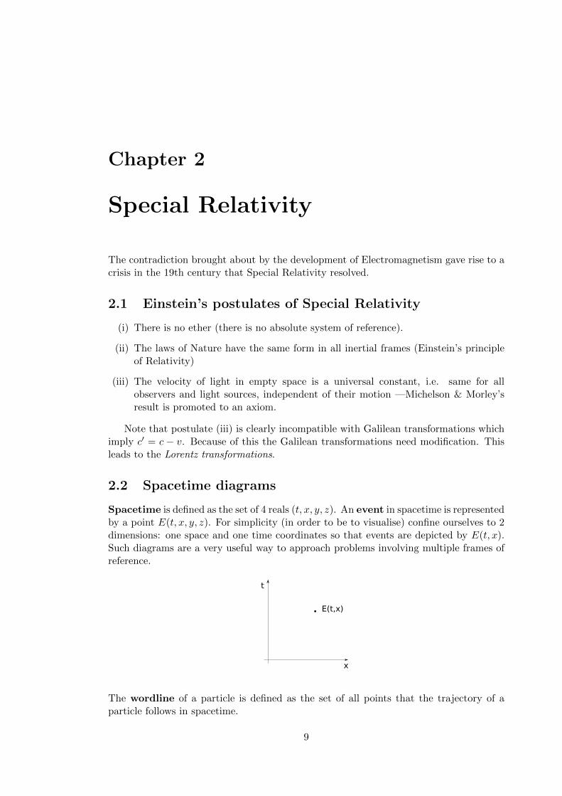
Spacetime is defined as the set of 4 reals (t, x, y, z). An event in spacetime is representedby a point E(t, x, y, z). For simplicity (in order to be to visualise) confine ourselves to 2dimensions: one space and one time coordinates so that events are depicted by E(t, x).Such diagrams are a very useful way to approach problems involving multiple frames ofreference.
�
�
������
The wordline of a particle is defined as the set of all points that the trajectory of aparticle follows in spacetime.
9
�
�
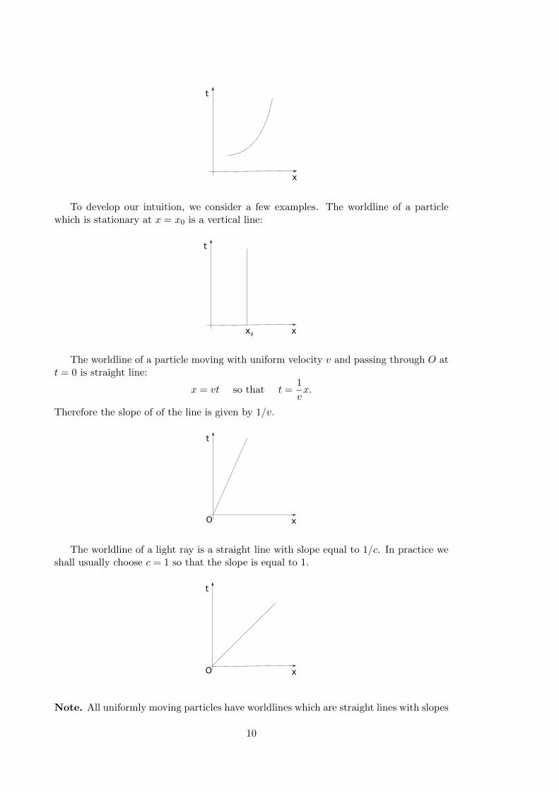
To develop our intuition, we consider a few examples. The worldline of a particlewhich is stationary at x = x0 is a vertical line:
�
���
The worldline of a particle moving with uniform velocity v and passing through O att = 0 is straight line:
x = vt so that t =1
vx.
Therefore the slope of of the line is given by 1/v.
�
��
The worldline of a light ray is a straight line with slope equal to 1/c. In practice weshall usually choose c = 1 so that the slope is equal to 1.
�
��
Note. All uniformly moving particles have worldlines which are straight lines with slopes
10
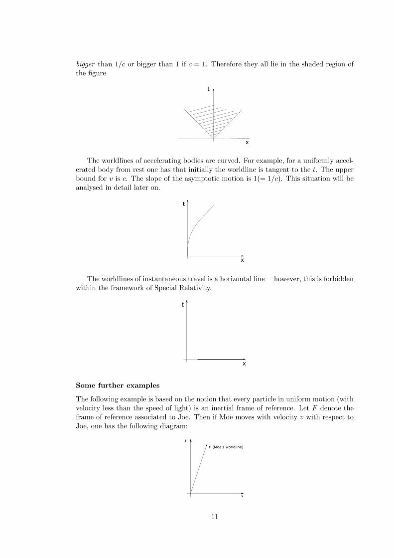
bigger than 1/c or bigger than 1 if c = 1. Therefore they all lie in the shaded region ofthe figure.
�
�
The worldlines of accelerating bodies are curved. For example, for a uniformly accel-erated body from rest one has that initially the worldline is tangent to the t. The upperbound for v is c. The slope of the asymptotic motion is 1(= 1/c). This situation will beanalysed in detail later on.
�
�
The worldlines of instantaneous travel is a horizontal line —however, this is forbiddenwithin the framework of Special Relativity.
�
�
Some further examples
The following example is based on the notion that every particle in uniform motion (withvelocity less than the speed of light) is an inertial frame of reference. Let F denote theframe of reference associated to Joe. Then if Moe moves with velocity v with respect toJoe, one has the following diagram:
�
�
������������ �����
11
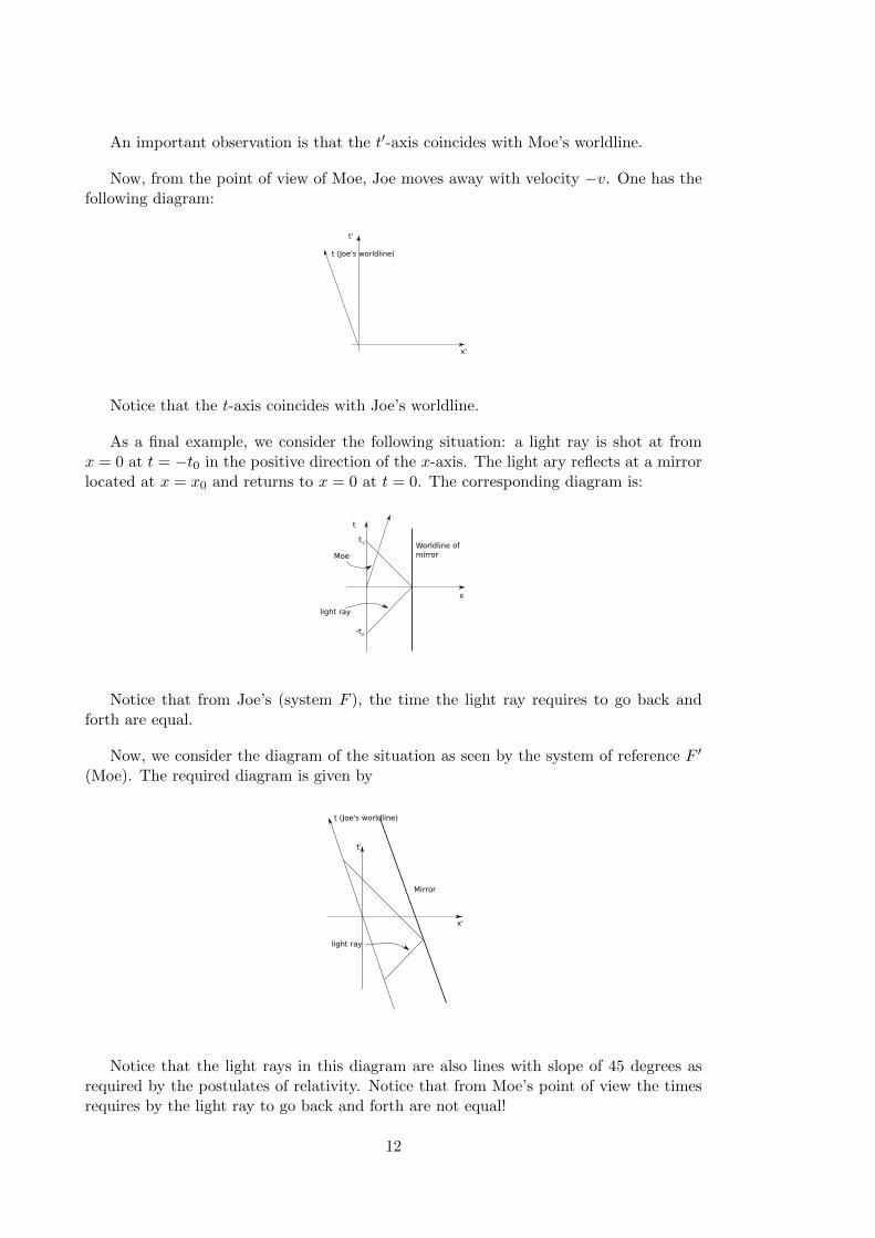
An important observation is that the t0-axis coincides with Moe’s worldline.
Now, from the point of view of Moe, Joe moves away with velocity �v. One has thefollowing diagram:
��
��
����������� �����
Notice that the t-axis coincides with Joe’s worldline.
As a final example, we consider the following situation: a light ray is shot at fromx = 0 at t = �t0 in the positive direction of the x-axis. The light ary reflects at a mirrorlocated at x = x0 and returns to x = 0 at t = 0. The corresponding diagram is:
�
�
���������� �����
���������
��
��
�
�
�
Notice that from Joe’s (system F ), the time the light ray requires to go back andforth are equal.
Now, we consider the diagram of the situation as seen by the system of reference F 0
(Moe). The required diagram is given by
��
��
����������� �����
������
���������
Notice that the light rays in this diagram are also lines with slope of 45 degrees asrequired by the postulates of relativity. Notice that from Moe’s point of view the timesrequires by the light ray to go back and forth are not equal!
12
2.3 Lorentz transformations (LT)
In this section we address the following question: what type of transformation does oneneed to ensure that the speed of light as measured by two inertial frames of reference Fand F 0 is equal?
In order to explore the consequences of this requirement, let us consider 2 inertialsystems of reference in standard configuration moving with relative velocity v. Supposea light ray is fired at x = 0 at t = 0. Futhermore, suppose that this light ray reaches(t, x). Let (t0, x0) be the coordinates of the event (t, x) as seen by F 0. As the speed oflight is c for both systems of reference, one has that
c = x/t, c = x0/t0.
For reasons that will become clear later in the chapter, it is covenient to rewrite theseexpressions as
0 = �c2t2 + x2, 0 = �c2t02 + x02.
Thus one has that�c2t2 + x2 = �c2t02 + x02. (2.1)
One can readily verify (by direct substitution) that the Galilean transformation t = t0,x = x0 � vt, cannot satisfy this condition. Thus, one needs to consider a di↵erent kindof transformation.
The so-called Lorentz transformations are given by:
x0 = �(x� vt), t0 = �⇣t� vx
c2
⌘, y0 = y, z0 = z. (2.2)
Remark. This is a particular case of a more general transformation with 10 parameters.These parameters are the 3 components of the velocity, 3 components of a shift of theorigin, 3 parameters of a rotation and a further parameter fixing the origin of the time.The set of these transformations forms a group. The transformation given by (2.2) is the1-parameter subgroup of this group called the special Lorentz group.
Remark. One can verify by direct substitution that the Lorentz transformation (2.2)satisfies
�c2t2 + x2 = �c2t02 + x02.
Remark. It is interesting what happens with the Lorentz transformations for low ve-locities. Using a Taylor expansion about 0, we recall
(1� x)�1/2 = 1 + 12x+O(x2).
It follows that
� ⇡ 1 + 12
v2
c2.
Now, if v ⌧ c, then v2/c2 ⇡ 0, so that � ⇡ 1. Hence, form the experssions for the Lorentztransformation one has that
t0 ⇡ t, x0 ⇡ x� vt.
That is, one recovers the Galilean transformations!
13
gamma=1/sqrt(1-v^2/c^2)
from
2.4 Clocks and rods in relativistic motion
We now consider the e↵ects of uniform motion on clocks and rods.
2.4.1 Time dilation
Consider F and F 0 in standard configuration. Let a standard clock be at rest in F 0 (atx = x0) and consider two events in this clock at times t01 and t02. Let also
�t0 = t02 � t01.
In order to find the interval �t as measured by F , recall that
�t = �(�t0 + v�x0).
However, �x0 = 0 as x02 = x01 = x0. Hence one obtains
�t = ��t0,
Since
� =1p
1� v2/c2> 1,
one finds that the interval as measured by F is longer.
There is a symmetry! Both observers say the same thing about each other!
2.4.2 Length contraction
This is also called the (Lorentz-Fitzgerald contraction). Consider F and F 0 in standardconfiguration. Let a rod of length �x0 be placed at rest along the x0-axis of F 0. To findthe length as measured in F , we must measure the distance between the two ends of therod simultaneously in F . Consider two events occurring simultaneously at the end pointsof the rod in F . Therefore one has �t = 0. Now, using
�x0 = �(�x� v�t)
one finds that
�x0 = ��x, or �x =1
��x0.
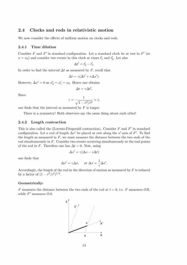
Accordingly, the length of the rod in the direction of motion as measured by F is reducedby a factor of (1� v2/c2)1/2.
Geometrically:
F measures the distance between the two ends of the rod at t = 0, i.e. F measures OB,while F 0 measures OA.
�
�
��
��
�
�
14
2.5 Paradoxes
These arise from an incautious view of the situation, and the fact that simultaneity meansdi↵erent things to di↵erent observers.
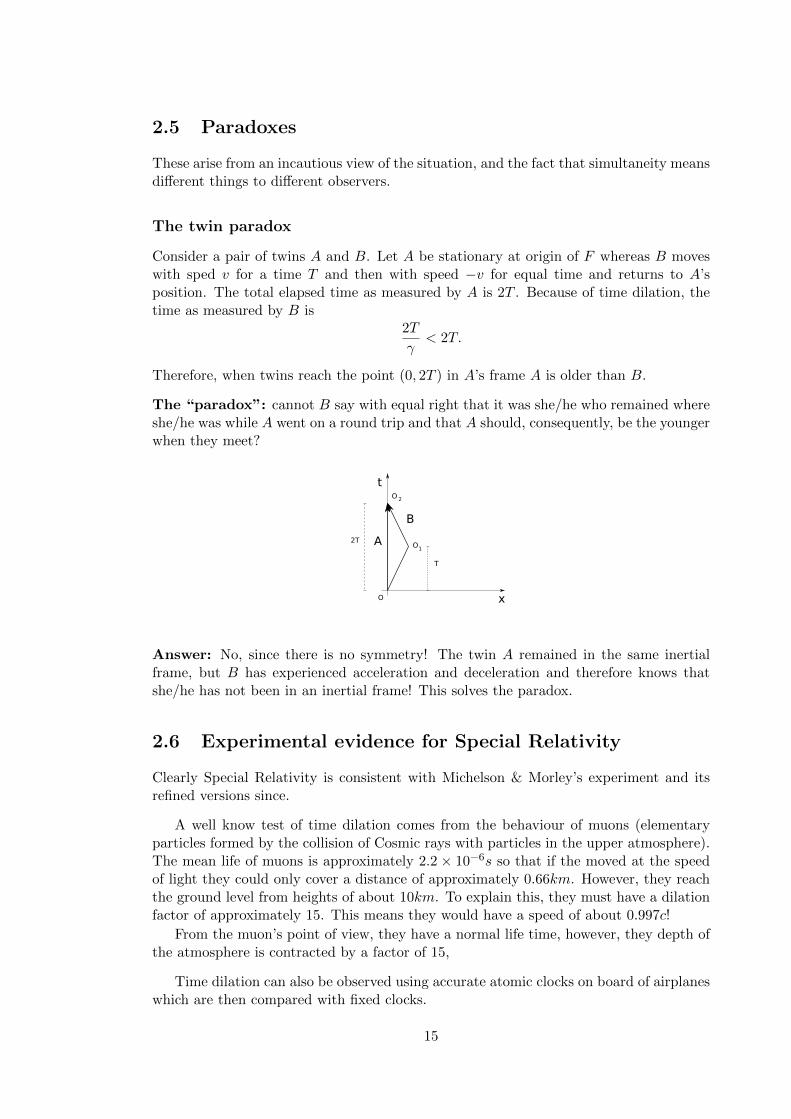
The twin paradox
Consider a pair of twins A and B. Let A be stationary at origin of F whereas B moveswith sped v for a time T and then with speed �v for equal time and returns to A’sposition. The total elapsed time as measured by A is 2T . Because of time dilation, thetime as measured by B is
2T
�< 2T.
Therefore, when twins reach the point (0, 2T ) in A’s frame A is older than B.
The “paradox”: cannot B say with equal right that it was she/he who remained whereshe/he was while A went on a round trip and that A should, consequently, be the youngerwhen they meet?
�
�
�
�
�
�
��
�
��
�
Answer: No, since there is no symmetry! The twin A remained in the same inertialframe, but B has experienced acceleration and deceleration and therefore knows thatshe/he has not been in an inertial frame! This solves the paradox.
2.6 Experimental evidence for Special Relativity
Clearly Special Relativity is consistent with Michelson & Morley’s experiment and itsrefined versions since.
A well know test of time dilation comes from the behaviour of muons (elementaryparticles formed by the collision of Cosmic rays with particles in the upper atmosphere).The mean life of muons is approximately 2.2 ⇥ 10�6s so that if the moved at the speedof light they could only cover a distance of approximately 0.66km. However, they reachthe ground level from heights of about 10km. To explain this, they must have a dilationfactor of approximately 15. This means they would have a speed of about 0.997c!
From the muon’s point of view, they have a normal life time, however, they depth ofthe atmosphere is contracted by a factor of 15,
Time dilation can also be observed using accurate atomic clocks on board of airplaneswhich are then compared with fixed clocks.
15
2.7 The inverse Lorentz transformation
In the previous section we discussed the Lorentz transformation which given the coor-dinates (t, x) of an event as seen by the system of reference F , allows to compute thecoordinates (t0, x0) as seen by F 0. Now, we are interested in the inverse transformationwhich given (t0, x0) allows to calculate (t, x). By symmetry, as F and F 0 are both iner-tial systems, the inverse transformation should have the same functional form. The keyobservation is then that if F sees F 0 moving with velocity v, then F 0 sees F moving withvelocity �v. Hence, the required transformtion is given by
t = �(t0 + v/c2x0),
x = �(x0 + vt0).
Remark. One could also have obtained the required expressions by inverting directly theoriginal Lorentz transformation formulae. This is, however, a much longer computation!A similar short argument an be used for the transformation formulae for the velocity andthe acceleration —see subsequent sections.
2.8 Hyperbolic form of the Lorentz transformations
This a convenient representation for showing the group properties of the Lorentz trans-formation.
The key idea is to replace the velocity parameter v by a hyperbolic parameter ↵ thatsatisfies the following:
cosh↵ = �, sinh↵ =v
c�, tanh↵ =
v
c.
We also require ↵ and v to have the same sign as cosh↵ = cosh(�↵).
The Lorentz transformation (2.2) becomes (hyperbolic form of the Lorentz transfor-
mation):
x0 = x cosh↵� ct sinh↵, (2.3a)
ct0 = �x sinh↵+ ct cosh↵, (2.3b)
y0 = y, (2.3c)
z0 = z (2.3d)
(2.3e)
Adding and subtracting x0 and ct0 as given by (2.3a) and (2.3b) one obtains
ct0 + x0 = e�↵(ct+ x), (2.4a)
ct0 � x0 = e↵(ct� x), (2.4b)
where it has been used that
cosh↵ =e↵ + e�↵
2.
To show that the Lorentz transformations form a group one needs to show:
(i) there exists an identity element;
16
(ii) for every Lorentz transformation there exists an inverse;
(iii) the composition of Lorentz transformations is a Lorentz transformation and thatthe composition is associative.
The most convenient way to verify the latter is to use the form given by (2.4a) and (2.4b)and then check one by one:
(i) One sees that there exists an identity Lorentz transformation corresponding to v(↵ = 0).
(ii) There exists an inverse Lorentz transformation with v = �v (↵ ! �↵).
(iii) Let F 00 move with velocity v2 (↵2) relative to F 0 and F 0 with velocity v1 (↵1)relative to F —all in standard configuration.
From (2.4a) and (2.4b) one has that
ct00 + x00 = e�↵2(ct0 + x0),
ct00 � x00 = e↵2(ct0 � x0),
y00 = y, z00 = z0
and
ct0 + x0 = e�↵2(ct+ x),
ct0 � x0 = e↵2(ct� x),
y0 = y, z0 = z.
It follows then that
ct00 + x00 = e�(↵1+↵2)(ct+ x),
ct00 � x00 = e(↵1+↵2)(ct� x),
y00 = y, z00 = z0,
which shows that the composition of Lorentz transformations is a Lorentz trans-formation and since the hyperbolic parameters add, one also has the associativity.
The previous discussion allows also to discuss the Special Relativity rule for the com-
position of velocities. Since the resultant of two Lorentz transformations with parameters↵1 and ↵2 is a Lorentz transformation with parameters ↵1+↵2, the corresponding relationbetween the velocity parameter of the transformation can be easily derived from
tanh↵ =v
c
by recalling that
tanh(↵1 + ↵2) =tanh↵1 + tanh↵2
1 + tanh↵1 tanh↵2.
Substituting for
tanh↵1 =v1c, tanh↵2 =
v2c, tanh↵1 + ↵2 =
v
c
17
one obtains
v =v1 + v2
1 + v1v2/c2(2.5)
where v is the velocity of F 00 relative to F —it represents the relativistic sum of collinear
velocities v1 and v2 along the x-axis. A generalisation of this rule will be discussed later.
Remark 1. Whenv1c
⌧ 1,v2c
⌧ 1,
then equation (2.5) takes the Galilean form
v = v1 + v2.
Remark 2. Since | tanh↵| < 1, it follows that v always satisfies |v| < c.
Appendix: Derivation of the Lorentz transformations
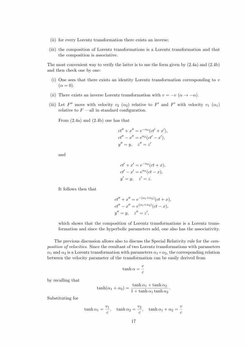
Consider two frames F and F 0 moving in standard configuration —i.e. O0 moves withspeed v along the x-axis relative to O. The worldline of O0 in the frame is given as inthe figure:
�
�
��
������
Let observers O and O0 carry clocks measuring t and t0 respectively such that whenO0 is at (t, vt) according to O, the clock at O0 registers t0 = �t, where � may be a functionof v —in this sense � carries all the e↵ect that the motion has on t. Note also that � = 1for Galilean transformations.
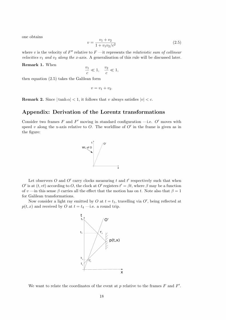
Now consider a light ray emitted by O at t = t1, travelling via O0, being reflected atp(t, x) and received by O at t = t4 —i.e. a round trip.
�
�
������
�
�
�
�
��
�
�
��
��
We want to relate the coordinates of the event at p relative to the frames F and F 0.
18
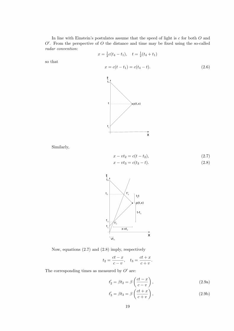
In line with Einstein’s postulates assume that the speed of light is c for both O andO0. From the perspective of O the distance and time may be fixed using the so-calledradar convention:
x = 12c(t4 � t1), t = 1
2(t4 + t1)
so thatx = c(t� t1) = c(t4 � t). (2.6)
�
�
������
�
�
�
�
�
Similarly,
x� vt2 = c(t� t2), (2.7)
x� vt3 = c(t3 � t). (2.8)
�
�
������
�
�
�
�
��
�
�
��
��
� ��
� �
� �
Now, equations (2.7) and (2.8) imply, respectively
t2 =ct� x
c� v, t3 =
ct+ x
c+ v.
The corresponding times as measured by O0 are:
t02 = �t2 = �
✓ct� x
c� v
◆, (2.9a)
t03 = �t3 = �
✓ct+ x
c+ v
◆, (2.9b)
19
where it has been used that t0 = �t. Therefore, the time and location of p(t, x) asmeasured by O0 is (using again the radar convention) is given by:
x0 = 12c(t
03 � t02) =
�c2(x� vt)
c2 � v2, (2.10a)
t0 = 12(t
03 + t02) =
�(c2t� vx)
c2 � v2, (2.10b)
where equations (2.9a) and (2.9b) have been used to obtain the second equalities in thelast pair of equations.
Note. The observer O0 is also assuming that the velocity of light is c. This assumptionis inconsistent with the Galilean transformations.
Eliminating x between (2.10a) and (2.10b) one obtains
t =1
�
✓t0 +
vx0
c2
◆. (2.11)
Now, the Relativity principle requires that we obtain the same result if we interchangex, x0 and t, t0 and let v ! �v. Applying this idea to equation (2.10b) and equating to(2.11):
t =�(c2t0 + vx0)
c2 � v2=
1
�
✓t0 +
vx0
c2
◆, (2.12)
so that
� =
✓1� v2
c2
◆1/2
.
Letting � ⌘ 1/�, the transformation for x0 can be found from (2.10a):
x0 = �(x� vt). (2.13)
Similarly for t from equation (2.10b):
t0 = �⇣t� vx
c2
⌘.
Finally, the coordinates y and z remain the same as there is no motion in these directions.
20
2.9 Further discussion on the Lorentz Transformations
2.9.1 Transformation formula for the velocity
Let F and F 0 be in standard configuration and moving with velocity v along the x-axis.For simplicity, we will restrict our attention to movements along the x-axis. Let V bethe velocity of a particle relative to F . To find V 0, the velocity relative to F 0 recall that:
V ⌘ dx
dt, (2.14a)
V 0 ⌘ dx0
dt0, (2.14b)
where the increment represents the distances and times between two events for the parti-cle relative to the two frames. Using the di↵erential form of the Lorentz transformations
dx0 = �(dx� vdt), dt0 = �(dt� v/c2dx),
in (2.14b) one obtains
V 0 =dx0
dt0=
�(dx� vdt)
�(dt� v/c2dx)=
V � v
1� V v/c2.
Remark. If v ⌧ c one finds that V 0 ⇡ V � v. That is, one recovers the Galileantransformation. Note also that if we do not restrict our attention to motion in the x-direction, then one computes the other components of the velocity V 0 in a similar mannerto above using dy0
dt0 and dz0
dt0 . Observe that in contrast with the Galilean transformations,the velocity components transverse to the direction of motion of frame F 0
are a↵ected by
the Lorentz transformation!
2.9.2 Transformation formula for the acceleration
A similar transformation for the acceleration can be found. Recall that
a ⌘ dV
dt, a0 ⌘ dV 0
dt0.
Starting from
V 0 =V � v
1� V v/c2
and calculating the di↵erential
dV 0 =dV
1� V v/c2+
V � v
(1� V v/c2)2v/c2dV,
one concludes that
dV 0 =1
�2dV
(1� vV/c2)2. (2.15)
Also, from the Lorentz transformation
dt0 = �(dt� v/c2dx),
it follows thatdV 0
dt0=
1
�3(1� vV/c2)3dV
dt.
21

Alternatively, on can write
a0 =1
�3(1� vV/c2)3a.
Notice that as a consequence of this formula, although acceleration is not an invariant,if the acceleration is zero in one inertial frame, then it is zero in all inertial frames. Hence,acceleration is in a certain sense absolute.
Remark. As before, if v ⌧ c, then one finds that a0 ⇡ a —the Galilean invariance ofacceleration.
2.10 The Minkowski spacetime
There are many ways to study Special relativity. here we take the geometrical approachdeveloped in 1908 by H. Minkoswki. This approach naturally leads to (and led Einstein!)to General Relativity.
To gain some intuition, start with the Euclidean geometry of the 2 dimensional planeand recall the transformation of coordinates corresponding to the rotation of Cartesianaxes by an angle ↵ in such a plane:
x0 = x cos↵+ y sin↵,
y0 = �x sin↵+ y cos↵,
where (x, y) and (x0, y0) correspond to the coordinates of the point p in the two frames.
�
�
��
��
��������������������
�
�
The transformation can be deduced from the diagram by observing that:
x0 = OA+AB = OA+ CD
= OC cos↵+ PC sin↵
= x cos↵+ y sin↵
y0 = PB = PD �BD
= PC cos↵�OC sin↵
= �x sin↵+ y cos↵.
Eliminating the rotation parameter ↵ by taking
x02 + y02 = (x cos↵+ y sin↵)2 + (�x sin↵+ y cos↵)2
= x2 + y2.
22
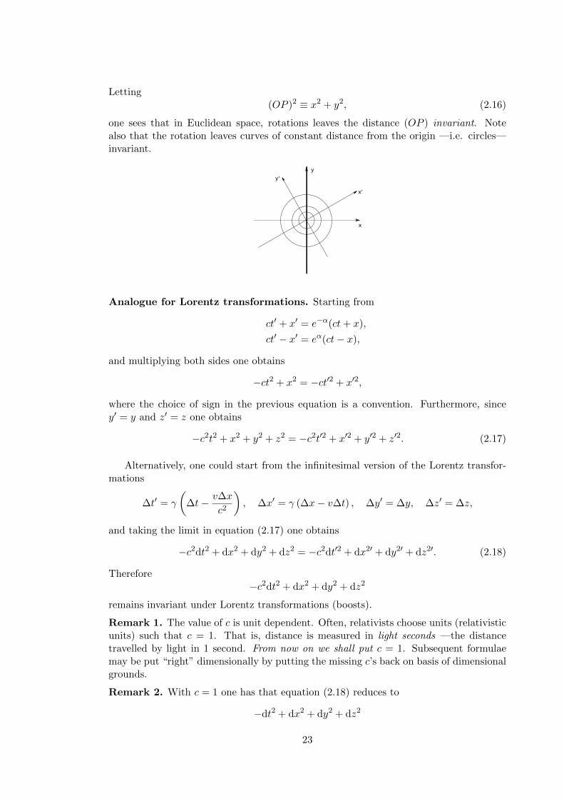
Letting(OP )2 ⌘ x2 + y2, (2.16)
one sees that in Euclidean space, rotations leaves the distance (OP ) invariant. Notealso that the rotation leaves curves of constant distance from the origin —i.e. circles—invariant.
�
�
��
��
Analogue for Lorentz transformations. Starting from
ct0 + x0 = e�↵(ct+ x),
ct0 � x0 = e↵(ct� x),
and multiplying both sides one obtains
�ct2 + x2 = �ct02 + x02,
where the choice of sign in the previous equation is a convention. Furthermore, sincey0 = y and z0 = z one obtains
�c2t2 + x2 + y2 + z2 = �c2t02 + x02 + y02 + z02. (2.17)
Alternatively, one could start from the infinitesimal version of the Lorentz transfor-mations
�t0 = �
✓�t� v�x
c2
◆, �x0 = � (�x� v�t) , �y0 = �y, �z0 = �z,
and taking the limit in equation (2.17) one obtains
�c2dt2 + dx2 + dy2 + dz2 = �c2dt02 + dx20 + dy20 + dz20. (2.18)
Therefore�c2dt2 + dx2 + dy2 + dz2
remains invariant under Lorentz transformations (boosts).
Remark 1. The value of c is unit dependent. Often, relativists choose units (relativisticunits) such that c = 1. That is, distance is measured in light seconds —the distancetravelled by light in 1 second. From now on we shall put c = 1. Subsequent formulaemay be put “right” dimensionally by putting the missing c’s back on basis of dimensionalgrounds.
Remark 2. With c = 1 one has that equation (2.18) reduces to
�dt2 + dx2 + dy2 + dz2
23
which, apart from the negative sign is very similar to the Euclidean distance in 4 dimen-sions
dl2 = dx2 + dy2 + dz2 + dw2.
Furthermore, they both remain invariant under coordinate transformations: Lorentztransformations and rotations, respectively. This invariant quantity is called the in-
terval ds2 (or line element) in a new type of geometry called the Minkowski geometry orspacetime. It is then described by
ds2 = �dt2 + dx2 + dy2 + dz2.
The latter measures the “distance” between events (t, x, y, z) and (t + dt, x + dx, y +dy, z + dz) in spacetime.
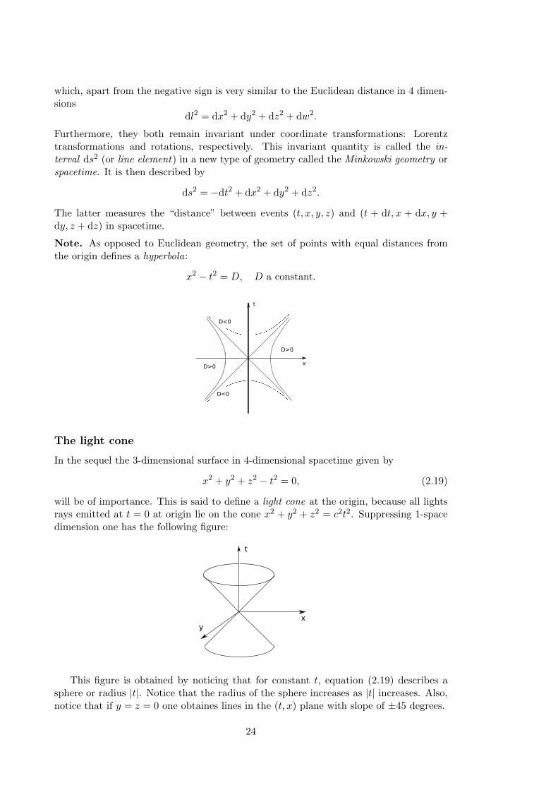
Note. As opposed to Euclidean geometry, the set of points with equal distances fromthe origin defines a hyperbola:
x2 � t2 = D, D a constant.
�
�
���
���
���
���
The light cone
In the sequel the 3-dimensional surface in 4-dimensional spacetime given by
x2 + y2 + z2 � t2 = 0, (2.19)
will be of importance. This is said to define a light cone at the origin, because all lightsrays emitted at t = 0 at origin lie on the cone x2 + y2 + z2 = c2t2. Suppressing 1-spacedimension one has the following figure:
�
��
This figure is obtained by noticing that for constant t, equation (2.19) describes asphere or radius |t|. Notice that the radius of the sphere increases as |t| increases. Also,notice that if y = z = 0 one obtaines lines in the (t, x) plane with slope of ±45 degrees.
24
2.10.1 Minkowski diagrams
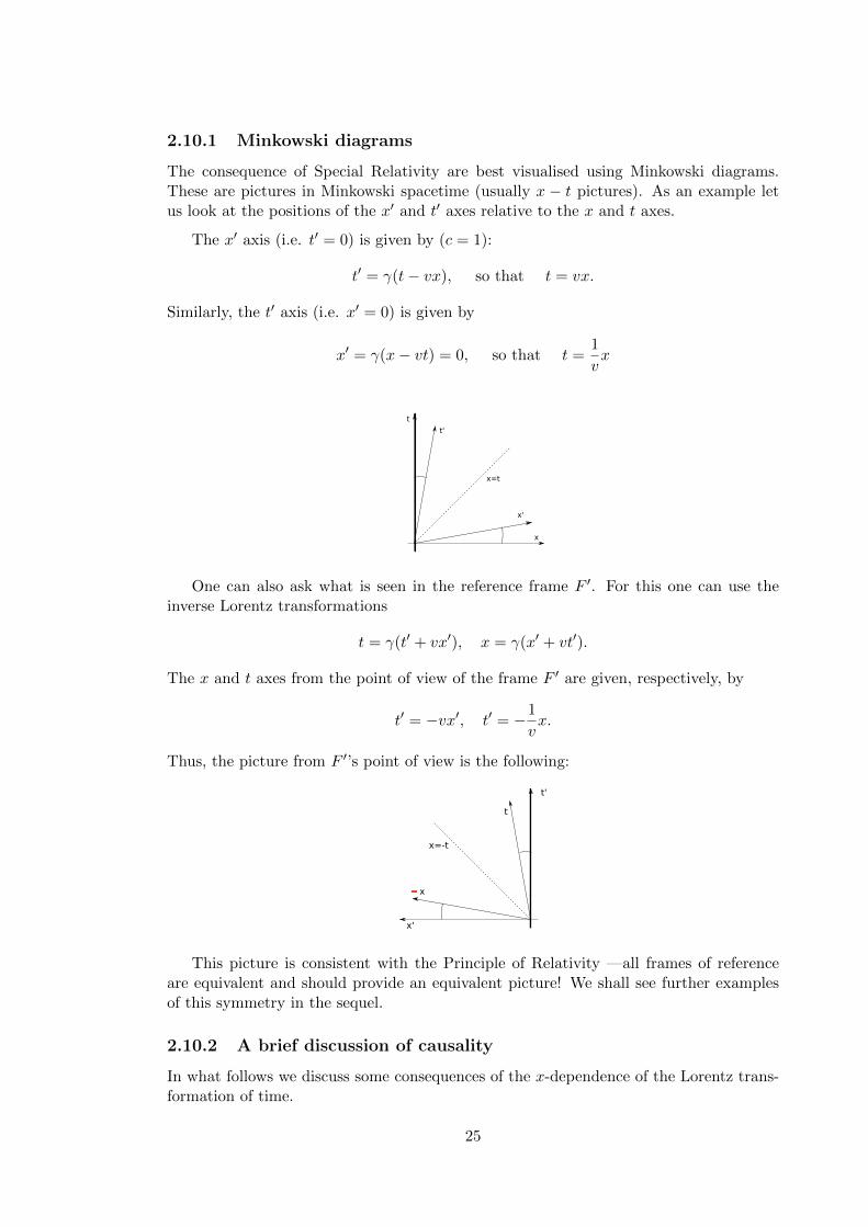
The consequence of Special Relativity are best visualised using Minkowski diagrams.These are pictures in Minkowski spacetime (usually x � t pictures). As an example letus look at the positions of the x0 and t0 axes relative to the x and t axes.
The x0 axis (i.e. t0 = 0) is given by (c = 1):
t0 = �(t� vx), so that t = vx.
Similarly, the t0 axis (i.e. x0 = 0) is given by
x0 = �(x� vt) = 0, so that t =1
vx
�
��
��
�
���
One can also ask what is seen in the reference frame F 0. For this one can use theinverse Lorentz transformations
t = �(t0 + vx0), x = �(x0 + vt0).
The x and t axes from the point of view of the frame F 0 are given, respectively, by
t0 = �vx0, t0 = �1
vx.
Thus, the picture from F 0’s point of view is the following:
����
��
��
�
�
This picture is consistent with the Principle of Relativity —all frames of referenceare equivalent and should provide an equivalent picture! We shall see further examplesof this symmetry in the sequel.
2.10.2 A brief discussion of causality
In what follows we discuss some consequences of the x-dependence of the Lorentz trans-formation of time.
25
-
�
��
��
���
��
��
�
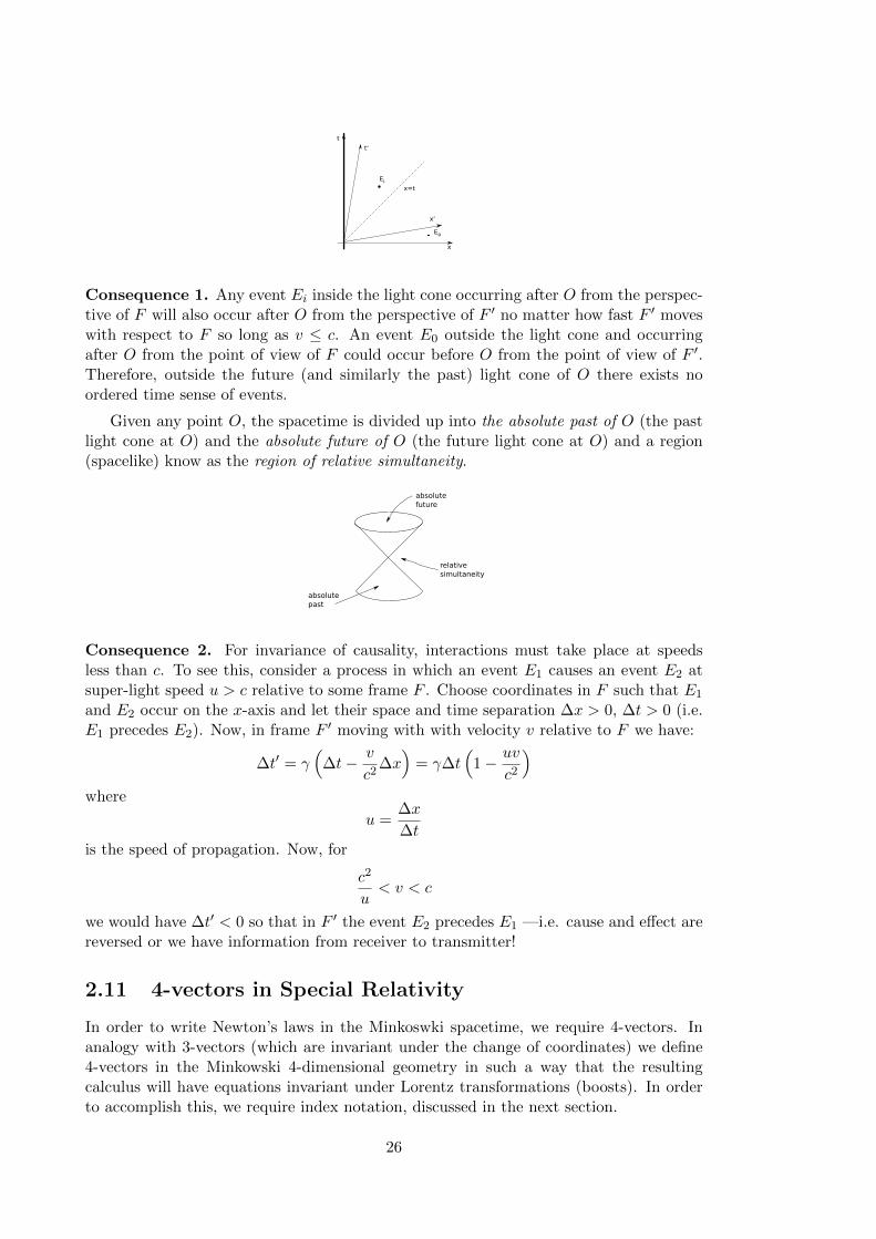
Consequence 1. Any event Ei inside the light cone occurring after O from the perspec-tive of F will also occur after O from the perspective of F 0 no matter how fast F 0 moveswith respect to F so long as v c. An event E0 outside the light cone and occurringafter O from the point of view of F could occur before O from the point of view of F 0.Therefore, outside the future (and similarly the past) light cone of O there exists noordered time sense of events.
Given any point O, the spacetime is divided up into the absolute past of O (the pastlight cone at O) and the absolute future of O (the future light cone at O) and a region(spacelike) know as the region of relative simultaneity.
�����������
�������������
������ �������������
Consequence 2. For invariance of causality, interactions must take place at speedsless than c. To see this, consider a process in which an event E1 causes an event E2 atsuper-light speed u > c relative to some frame F . Choose coordinates in F such that E1
and E2 occur on the x-axis and let their space and time separation �x > 0, �t > 0 (i.e.E1 precedes E2). Now, in frame F 0 moving with with velocity v relative to F we have:
�t0 = �⇣�t� v
c2�x⌘= ��t
⇣1� uv
c2
⌘
where
u =�x
�tis the speed of propagation. Now, for
c2
u< v < c
we would have �t0 < 0 so that in F 0 the event E2 precedes E1 —i.e. cause and e↵ect arereversed or we have information from receiver to transmitter!
2.11 4-vectors in Special Relativity
In order to write Newton’s laws in the Minkoswki spacetime, we require 4-vectors. Inanalogy with 3-vectors (which are invariant under the change of coordinates) we define4-vectors in the Minkowski 4-dimensional geometry in such a way that the resultingcalculus will have equations invariant under Lorentz transformations (boosts). In orderto accomplish this, we require index notation, discussed in the next section.
26
2.11.1 Index notation
In what follows let
(t, x, y, z) = (x0, x1, x2, x3),
where the index position is a convention —more about this later. Write
xa, (a = 0, 1, 2, 3)
for x0, x1, x2, x3 we may write (2.18) as
ds2 =3X
a=0
3X
b=0
⌘abdxadxb (2.20)
where ⌘ab is called the Minkowski metric tensor given by
(⌘ab) ⌘
0
BB@
�1 0 0 00 1 0 00 0 1 00 0 0 1
1
CCA
so that
⌘11 = ⌘22 = ⌘33 = 1, ⌘00 = �1,
while all other ⌘ab’s are zero.
In order to drop clumsy summations hereafter we will use the so-called Einstein
summation convention:
(i) Whenever an index is repeated (appears exactly twice) in a term, it is understoodto imply summation over that index over all its permissible values. In this courselower case Latin indices a, b, . . . take values 0, 1, 2, 3. Hence equation (2.20) maybe written
ds2 = ⌘abdxadxb.
(ii) Repeated indices as called dummy indices since they may be replaced by anotherindex (from the same alphabet!) not already used. For example:
ds2 = ⌘abdxadxb = ⌘cddx
cdxd.
(iii) To avoid ambiguity, no index should appear more than twice in the same expression.So
aibici
is not allowed!
(iv) Indices that occur only once in an expression (or terms of an equation) are calledfree indices. In an equation such indices match in every term. For example consider
AiBiCj = Dj .
Notice that i is a dummy index and that j is a free index.
27
ct
Examples
For simplicity in the following examples let the Latin lower case index take values 1, 2.
(1)AiBj = A1B1, A1B2, A2B1, A2B2
as i, j are free indices.
(2)
AiBi =2X
i=1
AiBi = A1B1 +A2B2,
as i is a dummy index.
(3)gij = g11, g12, g21, g22
as, again, i, j are free indices.
(4) In �ijk all indices are free. There are 8 terms: �111, �1
12; . . . .
(5) In Rijkl all indices are free and there are 16 terms: R1
111, R1112, R1
122, . . .
(6)
�ijkdxj
ds
dxk
ds= �i
lmdxl
ds
dxm
ds
as l, m are dummy indices while i is free.
(7) xaybzb = zaycyc.
(8) gijdxidxj = gmndxmdxn = g11(dx1)2 + g12dx1dx2 + g21dx2dx1 + g22(dx2)2.
2.11.2 4-vectors
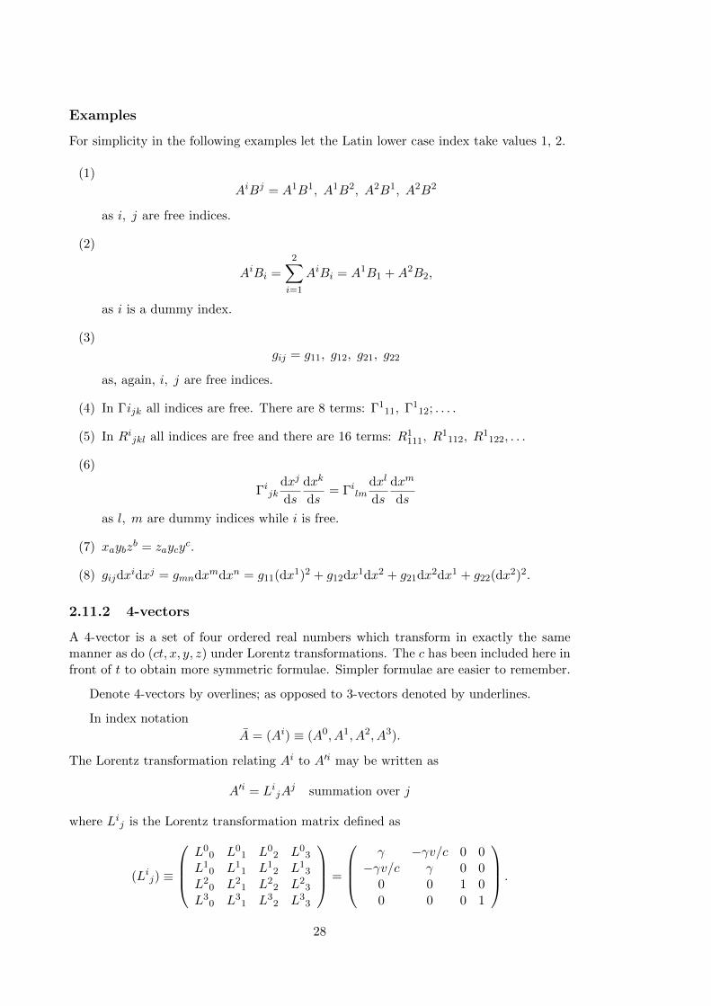
A 4-vector is a set of four ordered real numbers which transform in exactly the samemanner as do (ct, x, y, z) under Lorentz transformations. The c has been included here infront of t to obtain more symmetric formulae. Simpler formulae are easier to remember.
Denote 4-vectors by overlines; as opposed to 3-vectors denoted by underlines.
In index notationA = (Ai) ⌘ (A0, A1, A2, A3).
The Lorentz transformation relating Ai to A0i may be written as
A0i = LijA
j summation over j
where Lij is the Lorentz transformation matrix defined as
(Lij) ⌘
0
BB@
L00 L0
1 L02 L0
3
L10 L1
1 L12 L1
3
L20 L2
1 L22 L2
3
L30 L3
1 L32 L3
3
1
CCA =
0
BB@
� ��v/c 0 0��v/c � 0 0
0 0 1 00 0 0 1
1
CCA .
28
Check:
A00 = (�,��v/c, 0, 0)
0
BB@
A0
A1
A2
A3
1
CCA = �(A0 � v/cA1).
So it transforms like x0. One has a similar computation for A01.
Norm or magnitude of a 4-vector
It is defined by
|A|2 ⌘ (A1)2 + (A2)2 + (A3)2 � (A0)2 = ⌘abAaAb, (2.21)
which in analogy with the invariance of
x2 + y2 + z2 � t2 = |x|2, x = (t, x, y, z),
is invariant.
Exercise: Show by direct substitution that the norm of a 4-vector is invariant. Forsimplicity let c = 1. One has that
A00 = �(A0 � vA1),
A01 = �(A1 � vA0),
A02 = A2, A03 = A3.
Hence,
�(A00)2 + (A01)2 = �2(A1)2 + �2v2(A0)2 � 2�vA1A0 � �2(A0)2 � �2v2(A1)2 + 2�vA0A1,
= �2(A1)2(1� v2)� �2(A0)2(1� v2),
= (A1)2 � (A0)2.
Remark. Because of the negative sign in (2.21), the norm of a vector does not have tobe positive! A 4-vector A is said to be:
• timelike if |A|2 < 0,
• spacelike if |A|2 > 0,
• null if |A|2 = 0.
In Minkowski spacetime a null vector need not be a zero vector whose componentsare zero! Only in a space in which the norm is positive definite, it is true that |A|2 = 0implies A = 0.
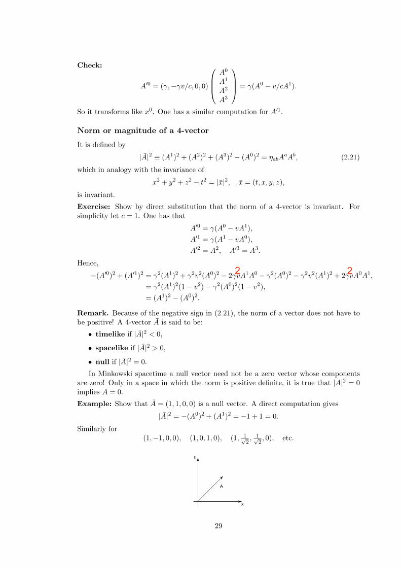
Example: Show that A = (1, 1, 0, 0) is a null vector. A direct computation gives
|A|2 = �(A0)2 + (A1)2 = �1 + 1 = 0.
Similarly for(1,�1, 0, 0), (1, 0, 1, 0), (1, 1p
2, 1p
2, 0), etc.
�
�
�
29
22
Scalar product
The scalar product of two 4-vectors A, B is defined by
A · B = ⌘abAaBb = �A0B0 +A1B1 +A2B2 +A3B3.
Notice that as a consequence of this definition |A|2 = A · A.
Example: Prove that A · B is invariant under Lorentz transformations: start with
(A+ B) · (A+ B) = |A|2 + |B|2 + 2A · B,
and note that |A|2, |B|2 and |A+ B|2 are all invariants. Hence, so is A · B.
Orthogonality
Two vectors are called orthogonal if A · B = 0.
Note 1. Because of the nature of the Minkowski geometry, two orthogonal 4-vectors donot appear orthogonal graphically.
Note 2. Null vectors are orthogonal to themselves (A · A = 0)!
Basic 4-vectors
In any frame F , there exist 4 basic vectors
e0 = (1, 0, 0, 0), e1 = (0, 1, 0, 0), e2 = (0, 0, 1, 0), e3 = (0, 0, 0, 1),
in terms of which any 4-vector A may be expressed:
A = Aiei = A0e0 +A1e1 +A2e2 +A3e3,
where Ai are the components of A
One can add and subtract 4-vectors pictorially like is done for 3-vectors.
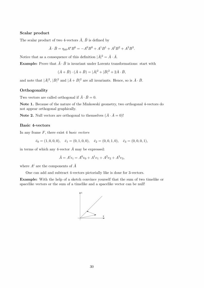
Example: With the help of a sketch convince yourself that the sum of two timelike orspacelike vectors or the sum of a timelike and a spacelike vector can be null!
�
�
30
2.12 Proper time
In order to develop relativistic dynamics one requires the analogues of
v =dx
dt, a =
dv
dt, F =
dp
dt,
etc. The problem is that in Special Relativity, t = x0 is not a scalar, so that we cannotjust carry d/dt over to Special Relativity.
The closest thing to dt which is a scalar is the proper time interval d⌧ defined by
d⌧2 ⌘ �ds2
c2= dt2 � dx2
c2� dy2
c2� dz2
c2.
In the previous definition the minus sign is included so that d⌧ and dt have the samesign! The name of proper time comes from the fact that a clock at rest with a movingparticle —i.e. in the particle’s rest frame where dx = dy = dz = 0— has d⌧ = d⌧ —i.e.it is equal to the time elapsed on the particle’s clock.
We employ ⌧ as the invariant measure of time for the particle.
2.13 4-velocity and 4-momentum
In order to express Newton’s laws in Special Relativity in an invariant way, we need toexpress them in terms of 4-vectors.
4-velocity
The 4-velocity of a particle is defined as a unit tangent to its Worldline:
U =dx
d⌧, U i =
dxi
d⌧.
In what follows, for simplicity we set c = 1.
Remarks:
(1) From the definition of d⌧ one finds that
ds2 = �d⌧2 = dx · dx
where dx = (dt, dx, dy, dz) so that
U · U = �1. (2.22)
So that 4-velocity as defined has unit length.
(2) From d⌧2 = dt2 � dx2 � dy2 � dz2 one finds that
✓d⌧
dt
◆2
= 1�✓dx
dt
◆2
�✓dy
dt
◆2
�✓dz
dt
◆2
= 1� v2,
where v denotes the 3-velocity relative to the frame F and v2 = v · v. Hence, oneconcludes that
dt
d⌧=
1p1� v2
= �(v) (c = 1).
31
Now, usingdx
d⌧=
dx
dt
dt
d⌧= �(v)v1, etc
one finds that
U =
✓dt
d⌧,dx
d⌧,dy
d⌧,dz
d⌧
◆= �(v)(1, v1, v2, v3),
or in shortU = �(v)(1, v). (2.23)
Note that the spatial part of U is essentially v (with a relativistic correction).
4-momentum
The 4-momentum is the natural analogue of the 3-momentum:
p = m0U ,
where m0 denotes the mass of the particle. From the definition it follows that
p · p = m20U · U = �m2
0,
where it has been used that U · U = �1. Also, using (2.23) one has
p = m0�(v)(1, v). (2.24)
It follows that the space part of (2.24) can be identified with the 3-momentum, whereby analogy m0� is called the the moving mass, or the apparent mass and m0 is referredas the rest mass.
Letm ⌘ m0�(v) =
m0p1� v2/c2
,
so that the time component of p is identified with the energy
E = m0c2�(v).
One reason for this identification comes from considering the limit for small v/c. Forv/c ⌧ 1 one has
E = m0c2�(v) = m0c
2(1� v2/c2)�1/2
⇡ m0c2 + 1
2m0v2,
where the binomial expansion has been used. Now, the second term is just the Newtoniankinetic energy (12m0v2). The first term (m0c2) is then interpreted as the rest mass energy.This is the famous equation
Erest = m0c2.
From the previous discussion one can write
p = (E, p), (2.25)
with p the 3-momentum and E the energy. From (2.24) one concludes that
p · p = (E, p) · (E, p) = �E2 + p · p.
Using (2.22) one concludes
E2 � p · p = m20, (c = 1).
32
4-acceleration
As one might expect, the 4-acceleration is the natural analogue of the 3-acceleration:
a =dU
d⌧=
d2x
d⌧2,
where U is the 4-velocity previously defined. Observe that by di↵erentiating the equationU · U = �1, it follows that
a · U = 0,
so that 4-acceleration and 4-velocity are found to be orthogonal.
2.14 Photons
The definition of 4-velocity given in the previous sections breaks down when applied toparticles moving with the speed of light (photons) since for light rays one has ds2 =�d⌧2 = 0. In this case one may choose another parameter � and define
k =dx
d�,
but again k · k = 0 since k is null. This also implies that p · p = 0 for photons as p is inthe direction of U . Now, recalling that p · p = �m2
0, it follows that m0 = 0 for photons.Hence, particles moving with the speed of light must be massless!
Consider a photon with 4-momentum p = (E, p) defined relative to some frame F .As seen before p · p = 0, so that one finds that
E2 � p2 = 0, or E = p.
Therefore, for photons the spatial 3-momentum and the energy are equal. In particular,if the photon moves along the x-direction one has that
px = E.
2.15 Doppler shift
Let F and F 0 be in standard configuration. Consider a photon of frequency ⌫ moving inthe x-direction relative to the frame F . Relative to the frame F 0 the energy of the photonmay be obtained using a Lorentz transformation. For this recall that p is a 4-vector andits energy is given by its t-component. So, from
p = (E, px), py = pz = 0,
one obtainsE0 = �(E � vpx), (c = 1). (2.26)
Also, recall that from Quantum Mechanics, a photon of frequency ⌫ has energy given byh⌫ where h denotes Planck’s constant:
h = 6.625⇥ 10�34Js.
33
Similarly, one has E0 = h⌫ 0. Substituting in (2.26) one obtains
h⌫ 0 =h⌫ � vpxp
1� v2. (2.27)
Furthermore, for such a photon E = px so that substituting into (2.27):
h⌫ 0 =h⌫ � vh⌫p
1� v2,
from which we can conclude
⌫ 0
⌫=
1� vp1� v2
=
r1� v
1 + v.
Adding the constant c:
⌫ 0
⌫=
s1� v/c
1 + v/c. (2.28)
This is the relativistic Doppler shift formula. Note that when v/c ⌧ 1, then using thebinomial expansion in (2.28) one obtains
⌫ 0
⌫⇡ 1� v/c,
which is the usual (non-relativistic) formula for the Doppler shift.
Remark. The Doppler shift has been fundamental in Cosmology to establish the ex-pansion of the Universe.
2.16 Relativistic dynamics
In Special Relativity Newton’s laws become:
First law. Remains unchanged, except that the straight lines referred to are now worldlines in Minkowski spacetime.
Second law. One has
F =dp
d⌧.
Third law. On basis of very precise experiments of Particle Physics, this remainsunchanged. That is, 4-momentum is conserved in collisions:
X
i
pi = constant,
where the sum is over the particles involved in the collision.
Note. Due to constancy of the time component, the conservation of energy with restmass is included in the balance!
2.16.1 Examples of relativistic collisions
This type of problems can be solved by equating components, squaring and then usingfurther properties of p.
34
Example 1
Consider 2 particles with rest masses m1 and m2 both moving along collinearly withspeeds u1 and u2. The particles collide and coalesce with the resulting particle movingin the same direction. The question is: what are the mass m and the speed u of theresulting particle?
Recall that p = m�(1, v) for a particle of 3-velocity v. The initial 4-momenta are:
p1 = m1�(u1)(1, u1, 0, 0),
p2 = m2�(u2)(1, u2, 0, 0).
The final 4-momentum is
p = m�(u)(1, u, 0, 0).
The conservation of -momentum is expressed by
p = p1 + p2. (2.29)
Squaring
p2 = p · p = p21 + p22 + 2p1 · p2. (2.30)
However,
|p1|2 = �m21, |p2|2 = �m2
2,
p1 · p2 = m1m2�(u1)�(u2)(�1 + u1u2).
Substituting in (2.30):
m =qm2
1 +m22 + 2m1m2�(u1)�(u2)(1� u1u2). (2.31)
Taking space and t-components of 4-momenta in equation (2.29)
m�(u)u = m1�(u1)u1 +m2�(u2)u2, (2.32a)
m�(u) = m1�(u1) +m2�(u2). (2.32b)
Dividing (2.32a) by (2.32b) one obtains
u =m1�(u1)u1 +m2�(u2)u2
m1�(u1) +m2�(u2). (2.33)
Remark. In the limit of u1 ⌧ c and u2 ⌧ c one has that �(u1), �(u2) ⇡ 1 and that(1� u1u2) ⇡ 1 so that (2.31) and (2.33) yield
m ⇡ m1 +m2,
u ⇡ m1u1 +m2u2m1 +m2
,
which are the classical version of the result.
35
Example 2
Consider the collision (scattering) of a photon of frequency ⌫ moving in the x-directionby an electron of mass me in a frame in which me is initially at rest. Assume that thesubsequent motion remains in the xy plane.
Before the collision the 4-momenta of the photon and electron are given, respectively,by
pp1 = (h⌫, h⌫, 0, 0),
pe1 = me�(0)(1, 0, 0, 0), �(0) = 1.
After the collision we have that
pp2 = (h⌫ 0, h⌫ 0 cos↵, h⌫ 0 sin↵, 0),
pe2 = me�(v)(1, v cos�, v sin�, 0),
where ⌫ 0 is the new photon frequency and ↵, � are as given in the figure.
The conservation of 4-momentum gives:
pp1 + pe1 = pp2 + pe2 .
Squaring:(pp1 + pe1 � pp2) · (pp1 + pe1 � pp2) = pe2 · pe2 . (2.34)
But,p2e1 = p2e2 = �m2
e, pp1 = pp2 = 0.
Substituting in (2.34) one obtains
pe1 · pp1 � pe1 · pp2 = pp1 · pp2 ,
from where�meh⌫ +meh⌫
0 = h2⌫⌫ 0(cos↵� 1),
and
sin2 ↵/2 =mec2
2h
✓1
⌫ 0� 1
⌫
◆. (2.35)
Similarly, to find � rewrite (2.34) as
(pp1 + pe2 � pp2) · (pp1 + pe2 � pp2) = pe1 · pe1 .
This example shows that the photon is deflected (or scattered) by and angle given by(2.35)
36
x
2 2
Chapter 3
Prelude to General Relativity
3.1 General remarks
At the time of the development of Special Relativity, physical interactions were supposedto be either gravitational or electromagnetic. Electromagnetism was already compatiblewith Special Relativity —i.e. invariant under Lorentz transformations. On the otherhand, Newton’s laws were not.
After the development of Special Relativity, what was needed was to construct arelativistic theory of gravity compatible with Special Relativity. The first attempts toconstruct such theory involved generalisations of Newton’s laws of gravity. For example,Nordstrom developed a theory which was Lorentz invariant but which is incompatiblewith the observations —it does not produce light bending.
Einstein in 1915 succeeded in constructing a theory which is both Lorentz invariantand which s compatible with predictions. This theory is called General Relativity. Inorder to develop General Relativity, we will require some ingredients of tensor calculus.To understand why this mathematical tool is required, we take first a look at some ofthe principles that underlie the theory.
3.2 The Equivalence Principle
The Equivalence Principle amounts to the following two statements:
(1) The (equation of) motion of a (spherically symmetric) test particle (one whoseown gravitational field may be neglected) in a gravitational field is independentof its mass and composition. The first verification of this statement is claimedto be Galileo’s Pisa bell tower experiment —although this particular experimentprobably never took place. More recent experiments like the one by Roll, Krotkovand Dicke (1964) have allowed to establish the equality to 1 part in 1011.
(2) Matter (as well as every form of energy) is acted on by (and is itself a source of)gravitational field. In other words, gravity couples everything.
An immediate consequence of (2) is that it is not possible to eliminate the force ofgravity in the same way that other forces may be eliminated, by for example, discon-necting power sources or by means of shielding as in the case of Faraday cages. The onlyother forces that behave in this way are the so-called fictitious forces (i.e. the centrifugal
37
and Coriolis forces) which arise when non-inertial frames of reference are employed. Theimportant point about these forces is that like gravity, they are proportional to the massof the particle. This led Einstein to suspect that these and the gravitational forces shouldenter the theory in the same way.
To get a better feeling for this, recall that the only way one can eliminate the force ofgravity is by choosing a freely falling frame —i.e. a comoving frame with the freely fallingparticle. This is can be visualised in the thought experiment (Gedankenexperiment) —sometimes referred to as the lift experiment.
The experiment suggests that there are no local experiments which distinguish non-rotating free fall in gravitational field from a uniform motion in a space free from gravita-tional fields. By local, here its is understood that the experiment is performed in a smallregion such that the variation of the gravitational field is negligible (observationally).This is another way of expressing the Equivalence Principle (all particles fall in the sameway). In this sense, Special Relativity is regained locally, in the sense that the laws ofPhysics in a freely falling frame are compatible with Special Relativity. Alternatively,one can say that spacetime is locally Minkowskian. Furthermore, for a global theory inthe presence of gravitation (i.e. GR), the geometry of spacetime must be such that itis locally Minkowskian. The natural tool to express and implement these ideas is theso-called tensor calculus.
3.3 Summary
In presence of gravitational fields there exist, in small regions (locally), preferred inertialframes (i.e. the non-rotating free falling frames) in which the special relativistic resultshold. On a large scale, on the other hand, there are no such preferred frames, and henceone needs to treat all large scale reference frames on the same footing. This suggeststhat the laws of nature should be formulated in such a way that they are invariant underarbitrary transformations of coordinates (i.e. reference frames), and not just the Lorentztransformations as was the case of Special relativity.
Interpreted physically, this is called the General Principle of Relativity as opposed tothe Special Principle of Relativity according to which laws of nature have the same formin inertial frames.
Interpreted mathematically, it is called the principle of General Covariance —theequations of Physics should have tensorial form.
38
Chapter 4
Di↵erential Geometry and tensorcalculus
In describing spacetime we wish our equations to be valid for any coordinates. Tensorialequations satisfy this property —hence their significance.
4.1 Manifolds and coordinates
Roughly speaking, a manifold is locally equivalent to a subset of n-dimensional Euclideanspace Rn —i.e. made of pieces that look like open sets in Rn and such that the piecesmay be glued together smoothly. This definition allows the notion of curved space to bemade precise.
Example. The surface of S2 (2-sphere) which is locally R2, even though non-locally itis curved and closed.
We view an n-dimensional manifold (also called spacetime in Relativity where n = 4)as a set of points each possessing a set of n coordinates (x0, x1, . . . , xn�1) where eachcoordinate ranges over a subset of the reals or the whole reals.
Note. The first coordinate is chosen to be x0 consistent with the notation in SpecialRelativity where x0 = t.
An important feature of general manifolds is that we cannot assume that the wholemanifold can be covered with a single (non-degenerate) coordinate system as it is thecase in Euclidean or Minkowski space.
Example. On the surface of the sphere S2, there are no coordinates which cover thewhole surface without degeneracy —i.e. with all images being well defined.
We shall have occasion to deal with space of dimension n � 2, but cases n = 2, 3, 4are of most interest.
Curves
A curve is defined as the set of points given by
xi = f i(u), i = 0, 1, . . . n� 1,
with u a parameter.
39
Subspaces
A subspace is defined as the set of points given by
xi = f i(u1, u2, . . . , um), i = 0, 1, . . . , n� 1,
with m < n. We speak of a subspace of dimension m < n.
We shall call a space of dimension n � 1 a hypersurface because like a surface in3-dimensional space it divides the n-dimensional space into 2 disjoint sets. This can beseen as follows: one can eliminate the n � 1 parameters for the n equations xi = f i
leaving
F (x0, x1, . . . , xn�1) = 0.
The points in the space not satisfying this equation fall into 2 classes —that for F > 0and that for F < 0.
4.2 Transformation of coordinates
Assume that well behaved coordinates exist —at least in patches. Since we wish our equa-tions to be valid for any coordinates, one has to analyse the changes from the coordinates(xa) to (x0a). That is, changes from
x0a = x0a(xb) ⌘ x0a(x0, . . . , xn�1) (4.1)
or inverse transformations of the type
xa = xa(x0b), (4.2)
where xa and x0a refer to coordinates of a point p relative to coordinates systems F andF 0 which are no longer assume to be inertial. We shall also assume that the functions xa
and x0a are di↵erentiable.
Di↵erentiating (4.1) one obtains
dx0a =@x0a
@x0dx0 +
@x0a
@x1dx1 + · · ·+ @x0a
@xn�1dxn�1,
or in a more compact form
dx0a =@x0a
@xbdxb (4.3)
where @x0a/@xb is the Jacobian of the transformation. For example, in 2 dimensions wehave
@x0a
@xb=
@x01
@x1@x01
@x2
@x02
@x1@x02
@x2
!.
Now, dxa may be treated as an infinitesimal displacement between two neighbouringpoints p(xa) and q(xa + dxa).
40
Example
We may describe the plane R2 by Cartesian coordinates (xi) = (x, y) or polar coordinates(x0a) = (r, ✓). We then have
x01 = r = (x2 + y2)1/2,
x02 = ✓ = arctan(x/y).
The inverse transformations are given by
x1 = x = r cos ✓ = x01 cosx02,
x2 = y = r sin ✓ = x01 sinx02.
4.3 Contravariant vectors
The infinitesimal displacement dxa is the prototype of a class of geometrical objectscalled contravariant vectors. A contravariant vector is defined as a set of n quantities V a
associated with a point p of the manifold which under change of coordinates transformaccording to
V 0a =@x0a
@xbV b, (4.4)
that is, in the same way as di↵erentials. Similarly, a contravariant tensor of rank or order2 is defined as a set of n2 quantities Uab which under a change of coordinates transformlike
U 0ab =@x0a
@xc@x0b
@xdU cd. (4.5)
In general, a contravariant tensor of rank k is as set of quantities V a1a2···ak whichtransform according to:
V 0a1a2···ak =@x0a1
@xb1@x0a2
@xb2· · · @x
0ak
@xbkV b1b2···bk .
Remark. Contravariant tensors of rank k are also called tensors of type (k, 0) —e.g. acontravariant vector V a is referred to as a tensor of rank (1, 0). An important specialcase is a tensor of rank 0 (type (0, 0)) also called a scalar or an invariant:
�0 = � at p.
4.4 Covariant and mixed tensors
Recall that given a real valued function (scalar field) � on the manifold one can definethe gradient of � by
@�
@xa
which is also a vector. If we transform this expression to another coordinate system {x0a}we have:
@�
@x0a=
@�
@xb@xb
@x0a
where the chain rule has been used. The latter is the prototype of a covariant vector orcovariant tensor of rank 1 or of type (0, 1).
41
More precisely, a covariant vector is defined as a set of n quantities Yb which transformaccording to:
Y 0a =
@xb
@x0aYb. (4.6)
Similarly, a covariant tensor of rank 2 (or type (0, 2)) can be defined by:
Y 0ab =
@xc
@x0a@xd
@x0bYcd.
More generally, a covariant tensor of rank k (or type (0, k)) is defined as:
Y 0a1a2···ak =
@xb1
@x0a1@xb2
@x0a2· · · @x
bk
@x0akYb1b2···bk .
Important remark! It is a convention to write contravariant tensors with raised indicesand covariant tensors with lowered indices.
Mixed tensors
One can also define geometric objects called mixed tensors. For example, the mixedtensor of rank 3 with 1 contravariant and 2 covariant indices (of type (1, 2)) satisfies
Z 0abc =
@x0a
@xe@xf
@x0b@xg
@x0cZe
fg.
Finally, one may define a mixed tensor of rank (p+q) of type (p, q) —i.e. p contravariantand q covariant indices. It can be written as
Za1···apb1···bq .
An example
If a contravariant vector and a covariant vector have, respectively, components Ai =(A1, A2) and Ai = (A1, A2) in Cartesian coordinates, find the components in polar coor-dinates. In this example one has
(x01, x02) = (r, ✓),
(x1, x2) = (x, y).
Also
x = r cos ✓, y = r sin ✓,
r = (x2 + y2)1/2, ✓ = arctan(y/x).
Recall also that
A0i =@x0i
@xjAj , A0
i =@xj
@x0iAj .
Thus, one has to compute@x0i
@xj,
@xj
@x0i.
42
A lengthy but straightforward calculation gives:
@x1
@x01=
@x
@r= cos ✓,
@x2
@x01=
@y
@r= sin ✓,
@x1
@x02=
@x
@✓= �r sin ✓,
@x2
@x02=
@y
@✓= r cos ✓,
and
@x01
@x1=
@r
@x=
x
r,
@x01
@x2=
@r
@y=
y
r,
@x02
@x1=
@✓
@x= � y
r2,
@x02
@x2=
@✓
@y=
x
r2.
For the contravariant tensor Aa one has then that
A01 =@x01
@xaAa =
@r
@xA1 +
@r
@yA2 =
1
r(xA1 + yA2),
A02 =@x02
@xaAa =
@✓
@xA1 +
@✓
@yA2 =
1
r2(�yA1 + xA2).
For the covariant tensor Aa one has
A01 =
@xa
@x01Aa =
@x
@rA1 +
@y
@rA2 = A1 cos ✓ +A2 sin ✓,
A02 =
@xa
@x02Aa =
@x
@✓A1 +
@y
@✓A2 = �r sin ✓A1 + r cos ✓A2.
This example shows, in particular, that contravariant and covariant tensors are di↵erentgeometric objects.
Remark 1. In Cartesian coordinates there exists no distinction between covariant andcontravariant vectors and that is why one could get away with thinking that they are thesame. In general, specially in spaces in which no global Cartesian coordinates exist, it isimportant to recognize that even though @�/@xa is a vector, it is not the same kind ofvector as dxa.
Remark 2. Tensors as we have defined them are a set of components at a point of themanifold with particular transformation rules.
Remark 3. A tensor field is an association of a tensor of the same rank to every pointof a manifold. A tensor field is called continuous or di↵erentiable if its components insome coordinate system are continuous or di↵erentiable functions of the coordinates. Ifthey are C1, they are called smooth.
Remark 4. A vector is a tensor with one index. A scalar is a tensor with no indices.Not all geometric objects are tensors.
Remark 5. The importance of tensors in Mathematical Physics and Relativity lie in thefact that a tensor equation which holds in one coordinate system holds in all coordinatesystems. For example, suppose that in unprimed coordinates one has that
Vab = Wab.
43
The transformation to primed coordinate is given by
V 0ab =
@xc
@x0a@xd
@x0bVcd,
W 0ab =
@xc
@x0a@xd
@x0bWcd,
so that
V 0ab = W 0
ab.
Remark 6. The Kronecker delta �ij is defined by
�ij =
⇢1 if i = j0 if i 6= j
Now, to prove that �ij is a tensor of type (1, 1) we note that if were one it should transformas:
�0ij =@x0i
@xa@xb
@x0j�ab.
Now, substituting in the right hand side for �ab
@x0i
@xb@xb
@x0j=
@x0i
@x0j= �0ij .
4.5 Tensor algebra
To write equations in a covariant (tensorial) form, we need to build new tensors fromgiven ones. The following simple algebraic operations are useful. The trick is always toshow that a given object transforms like a tensor.
4.5.1 Addition (linear combination)
The linear combination of tensors of the same type is a tensor of the same type. As afirst example we show that if W a
b and Zab are tensors of type (1, 1), then so is
V ab ⌘ ↵W a
b + �Zab,
with ↵, � scalars. To see this notice that
V 0ab = ↵W 0a
b + �Z 0ab
= ↵@x0a
@xe@xf
@x0bW e
f + �@x0a
@xe@xf
@x0bZe
f ,
=@x0a
@xe@xf
@x0bV e
f ,
which transforms as a tensor of type (1, 1).
44
4.5.2 Direct product
The product of 2 tensors of type (p1, q1) and (p2, q2) is a tensor of type (p1 + p2, q1 + q2)provided none of the indices are the same. As an example, if V a
b and W c are tensors oftype (1, 1) and (1, 0) respectively, show that
Zabc ⌘ V a
bWc,
is a tensor of type (2, 1). To see this
Z 0abc = V 0a
bW0c,
=@x0a
@xe@xf
@x0bV e
f@x0c
@xhW h,
=@x0a
@xe@xf
@x0b@x0c
@xhZe
fh.
4.5.3 Contraction
Setting an upper and a a lower index equal and summing over its values results in anew tensor with the two indices absent. That is, one passes from a tensor of rank (p, q)to one of rank (p � 1, q � 1). For example if Za
bcd is a tensor of type (3, 1), show that
Zac ⌘ Zabcb is a tensor of type (2, 0). To see this write
Z 0ac = Z 0abcb =
@x0a
@xe@xf
@x0b@x0c
@xg@x0b
@xhZe
fgh.
However, note that@xf
@x0b@x0b
@xh=
@xf
@xh= �f h,
so that
Z 0ac =@x0a
@xe@x0c
@xgZeg.
The latter is a tensor of rank (2, 0).
4.5.4 Detection of tensors
Suppose one has a geometric object with indices. How does one decide if it is a tensor?As an example, if Bi is an arbitrary contravariant vector and AiBi is an invariant scalar,prove that Ai is a covariant vector. To see this write
AiBi = A0
iB0i
= A0i
✓@x0i
@xjBj
◆
so that ✓Aj �A0
i@x0i
@xj
◆Bj = 0,
and since Bj is arbitrary this implies
Aj = A0i@x0i
@xj,
so that Aj is indeed contravariant.
45
—
4.5.5 Symmetric and antisymmetric tensors
A tensor Aij is said to be symmetric if
Aij = Aji,
and antisymmetric (or skew) ifAij = �Aji.
Remark 1. For tensor this property is preserved under coordinate transformationsbecause
Aij ±Aji
are tensors by the addition property, so if they vanish in one coordinate system then theyvanish in all coordinate systems.
Remark 2. In n dimensions a symmetric tensor Aij has12n(n+1) independent compo-
nents and an antisymmetric has 12n(n� 1) independent components.
Remark 3. Any rank 2 tensor can be expressed as the sum of a symmetric and anantisymmetric (skew) parts:
Aij =12(Aij +Aji) +
12(Aij �Aji),
= A(ij) +A[ij].
For a tensor of higher rank one says that it is symmetric (or skew) with respect to apair of indices if interchanging the indices does not change the components (changes thesign). The indices involved must be both “upstairs” or “downstairs”. For example
R[ab][cd]
implies
Rabcd = �Rbacd,
Rabcd = �Rabdc,
Rabcd = Rbadc.
For rank 3 tensors, we may also symmetrize/anti-symmetrize as follows:
A(ijk) =16(Aijk +Ajki +Akij +Ajik +Akji +Aikj),
A[ijk] =16(Aijk +Ajki +Akij �Ajik �Akji �Aikj).
46
Rabcd =
4.6 Manifolds with metric
So far, we have defined tensor fields on manifolds with the intention of writing downlaws of physics in a coordinate-free manner. In particular, tensorial equations which holdin one coordinate system hold in all cordinate systems. However, to write down anyequation involving dynamics (of particles, say), we will need to define di↵erentiation onour manifold. In order to accomplish this, we start by introducing a notion of distance.
There are some reasons that lead us to introduce further structure on a manifold.Namely,
(i) from the Equivalence principle, spacetime is locally Minkowskian;
(ii) the need of an notion of parallelism based on the idea of length;
(iii) finding a relation between covariant and contravariant tensors.
In order to accomplish these point we introduce the notion of metric. This essentiallyamounts to defining the distance between two neighbouring points xa and xa + dxa
through an expression of the form
ds2 = gab(x)dxadxb (4.7)
where ds2 is called the line element or interval and gab is the metric tensor. A manifoldwith such a metric defined on it is called, unsurprisingly, a manifold with metric.
Remark 1. The tensor gab is a tensor of type (0, 2). This follows immediately from thescalar nature of ds2 and the fact that dxa is a contravariant tensor —this from the tensordetection method. To see this recall that
dxa =@xa
@x0cdx0c,
so that
ds2 = gabdxadxb
= gab@xa
@x0c@xb
@x0edx0cdx0e
= g0cedx0cdx0e,
where
g0ce = gab@xa
@x0c@xb
@x0e.
The later is precisely the transformation law for a tensor (0, 2).
Remark 2. In order for (4.7) to determine gab uniquely, gab must be symmetric. Notethat if gab is symmetric, then it can always be diagonalised. Let �i, i = 0, . . . N denotethe eigenvalues of gab. If all the eigenvalues of gab are positive, then the metric gab willbe said to be a Riemannian metric and the manifold will be said to be a Riemannian
manifold. If one of the eigenvalues is negative and the remaining positive, then the metricwill be said to be Lorentzian —this is the case of relevance in Relativity. The number ofpositive eigenvalues minus the number of negative eigenvaues is calld the signature. Inlight of this, we state the following result:
47
Theorem 1. In the diagonal form of gab the number of components equal to +1 and to
�1 do not change under coordinate transformations. The di↵erence between these two is
called the signature of the metric.
For example, the signature of the Minkowski metric from Special Relativity is +2,while the standard Euclidean metric in R4 has signature 4.
Remark 3. Euclidean space with
ds2 = dx2 + dy2 + dz2 + dw2
is an example of a Riemannian manifold. On the other hand, Minkowski space with
ds2 = �dt2 + dx2 + dy2 + dz2
is a special case of Lorentzian manifold. Note that in both examples, the coe�cientsgab are constants. We also note that the Minkowski metric can be written is sphericalcoordinates as:
ds2 = �dt2 + dr2 + r2d✓2 + r2 sin2 ✓d'2.
Definition (4.7) allows us to generalize many of the notions we had in Minkowskispace.
Norm of a contravariant vector V a
This is defined via|V |2 ⌘ gabV
aV b.
If |V |2 > 0 ( or |V |2 < 0) for all vectors V a, the metric is called positive definite (ornegative definite) —this is the Riemannian case. Otherwise it is called indefinite —thisincludes the Lorentzian case.
Scalar product between two vectors Aa and Bb
This is defined viaA ·B ⌘ gabA
aBb.
If gabAaAb = 0, then Aa and Bb are said to be orthogonal.
Null vectors
For indefinite metrics there are vectors that are orthogonal to themselves. That is,
gabAaAb = 0.
Contravariant form of the metric
Let g ⌘ det(gab). If g 6= 0, then the inverse of gab, gab can be defined by
gabgac = �b
c.
Defined in this way, gab is a contravariant tensor of rank 2.
As an example, consider the case when gab is diagonal —that is, gab = 0 a 6= b. Thenone can show that for g 6= 0,
g11 =1
g11, g22 =
1
g22, · · · , gab = 0, a 6= b.
48
with entries +/- 1
Lowering and raising of indices (index gymnastics)
One can use gab and gab to lower and raise indices for general tensors via the rules:
T ······a ⌘ gabT
···b··· (a is the raised index)
T ···a··· ⌘ gabT ···
···b (a is the raised index).
For example
gacWab = Wc
b,
T ab = gacTcb = gacgbdTcd.
Quite crucially, one can see that the operation of lowering and raising indices does notadd extra information in the tensors. For example, given
V b = gbaVa,
one has thatgebV
b = gebgbaVa = �e
aVa = Ve.
Thus, if one raises an index and then one lowers it, one receovers the orginal tensor.
Connection between contravariant and covariant vectors
So far, covariant and contravariant tensors have remained unrelated. The metric can betaken as the mapping between contravariant and covariant tensors:
Va = gabVb, V a = gabVb.
For Euclidean space in Cartesian coordinates
gab =
0
BBBB@
1 0 · · · 0
0. . .
. . ....
.... . .
. . . 00 · · · 0 1
1
CCCCA.
This is the reason why in this case there is no distinction between covariant and con-travariant tensors.
Remark 1. Raising and lowering of indices enable us to write equations with indices inany position. It is for that reason that one writes a blank space above each lower indexand below each upper index. For example the contravariant version of
Gab = Tab
isGab = T ab.
Remark 2. In a general 4-dimensional Lorentzian manifold with a metric gab with g 6= 0there exist “locally inertial coordinates” as defined by the following theorem:
Theorem 2. Given any point p of a Lorentzian manifold, it is always possible to find
coordinate transformations with origin at p such that
gab(x) = ⌘ab +O(x2).
That is, gab is approximately the Minkowski metric to second order:
gab(p) = ⌘ab, @cgab(p) = 0, @c@dgab(p) 6= 0.
49
4.7 Derivatives and connections
Most dynamical laws of Physics are expressible as di↵erential equations. A coordinateindependent formulation of such laws requires a coordinate independent definition ofderivative.
It is recalled that the partial derivative of a scalar function is a tensor, however, asit will be seen the partial derivative of a higher rank tensor is not tensorial. To see this,consider a contravariant tensor V a. Its transformation law is given by
V 0b =@x0b
@xaV a.
Di↵erentiating with respect to x0c one obtains
@V 0b
@x0c=
@2x0b
@xd@xa@xd
@x0cV a +
@V a
@xd@xd
@x0c@x0b
@xa,
where the chain rule@
@x0c=
@xd
@x0c@
@xd
has been used. The second term in the right hand side is what one would expect if@V a/@xd were a tensor of second rank. It is the first term the one that destroys thetensorial character!
One needs a definition of derivative which renders tensors. That is, a modificationra of @a with produces tensors. If rc is to be a derivative one needs the following to besatisfied:
rcf = @cf,
rc(Ab +Bb) = rcAb +rcBb, (linearity)
rc(AaBb) = (rcAa)Bb +Aa(rcBb), (Leibniz rule).
The simplest modification of @c that satisfies the above requirements is the following:
rcVa ⌘ @cV
a + �abcV
b, (4.8)
where the quantity �abc which has N3 components is called the connection or sometimes
the a�ne connection; for General Relativity, typically N = 4. Note that the particularform of �a
bc has not yet been identified.
Notation. Sometimes equation (4.8) and similar expressions are written as
V a;c = V a
,a + �abcV
b,
where we have introduced the colon-semicolon notation:
V a;c ⌘ rcV
a, @cVa ⌘ V a
,a.
Also notice that the di↵erentiation index c comes last in the connection �abc. This
notation will sometimes used in these notes to so that expressions are more compact andeasier to read.
50
c
c
Tensorial character of the covariant di↵erentiation
We will now choose a transformation law for �abc making rcV a a tensor of type (1, 1).
Recall that we already have seen that from
V 0b =@x0b
@xaV a,
it follows that
@cV0b =
@2x0b
@xd@xa@xd
@x0cV a +
@V a
@xd@xd
@x0c@x0b
@xa.
Now, from the definition (4.8) one has
rcV0a = @cV
0a + �0abcV
0b,
so that (switching a and b in the expression above for @cV 0b)
rcV0a =
@V b
@xd@xd
@x0c@x0a
@xb+
@2x0a
@xd@xb@xd
@x0cV b + �0a
bc@x0b
@xfV f . (4.9)
Now, to ensure that rcV 0a transforms as a tensor of type (1, 1) one requires
�0abc =
@x0a
@xd@xe
@x0b@xf
@x0c�d
ef � @2x0a
@xd@xl@xd
@x0c@xl
@x0b.
The second term in this last expression is to cancel the second term in (4.9) by notingthat
@xl
@x0b@x0b
@xf= �lf
and that f and b are dummy indices that can be interchanged:
�✓
@2x0a
@xd@xf@xd
@x0c@xl
@x0b
◆@x0b
@xfV f = � @2x0a
@xd@xf@xd
@x0cV f .
Remark 1. Clearly, �abc is not a tensor. Its transformation law is not homogeneous.
Remark 2. By insisting that the covariant derivative of a scalar is the partial derivativeand that the covariant di↵erentiation satisfies the Leibnitz rule, one can obtain a formulafor the covariant derivative of a covariant tensor:
rbVa = @bVa � �cabVc.
In general, one has that
rcTa···
b··· = @cTa···
b··· + �adcT
d···b··· + · · ·� �d
bcTa···
d···.
4.8 Parallel transport
A tensor V a is said to be parallely transported along W b if
W brbVa = 0.
Now, recall that one way of characterising straight lines in Euclidean space is as curveswhose tangent vectors are parallely transported at every point —i.e. they are autopar-allels. The notion defined above can be used to define the analogue of straight lines in
51
more general manifolds. Such curves are referred to as a�ne geodesics —i.e. curvesalong which the tangent vector is propagated parallely to itself. We remark that thisdefinition can also be used to define a notion of shortest distance on a manifold usingthe metric, but we shall defer this to a later point in the course.
Letting W b to be tangent to a geodesic, one has that
W brbWa = 0,
from whereW b@bW
a + �acbW
cW b = 0.
If the curve is parametrised by �, then
W b =dxb
d�,
and since
W b @
@xb=
d
d�
✓⌘ dxb
d�
@
@xb
◆,
so thatd
d�
✓dxa
d�
◆+ �a
bcdxc
d�
dxb
d�= 0,
and finally thatd2xa
d�2+ �a
bcdxc
d�
dxb
d�= 0. (4.10)
Note. From the existence and uniqueness theorems for ordinary di↵erential equations,it follows that corresponding to every direction at a point, there exists a unique geodesicpassing through the point. The initial conditions are
� = �0, xa0 = xa(0), W a0 =
dxa
d�(0).
Example. Show that changing the geodesic parameter � to � in such a way that � =�(�), the geodesic equation only keeps its form (4.10) in � if � = a�+ b.
To see this recall thatdxa
d�=
dxa
d�
d�
d�,
so thatd2xa
d�2=
d2xa
d�2
✓d�
d�
◆2
+dxa
d�
d2�
d�2.
Substituting into equation (4.10) one gets✓d2xa
d�2+ �a
bcdxc
d�
dxb
d�
◆✓d�
d�
◆2
+dxa
d�
d2�
d�2= 0,
which only has the form of (4.10) if
d2�
d�2= 0.
That is, if� = a�+ b.
A parameter of this form is called an a�ne parameter.
Remark. Note that only the symmetric part of the connection coe�cient is required inthe geodesic equation (4.10).
52
4.9 The Levi-Civita connection
Up to now the connection �abc has remained undefined. We will see now that given
a metric gab, there is a preferred (canonical) connection. For this we will impose twoconditions on the connection.
No torsion condition
Let � be as scalar. The usual partial derivatives acting on a scalar commute. That is,
@a@b� = @b@a�.
This is, in general, not the case for covariant derivatives. Recall that
rb� = @b�,
so that
rarb� = @a@b�� �eba@e�,
rbra� = @b@a�� �eab@e�.
Thus, the covariant derivatives commute if and only if
�cab = �c
ba = �c(ab).
This property has a nice geometric interpretation. namely, that the parallelogram formedby the parallel propagation of two infinitesimal displacements closes.
Constancy of the inner product upon parallel propagation
The metric gab imposes a natural condition on the parallel transport. Given two vectorsV a and W b one can require that their inner product gabV aW a remains unchanged if weparallel transport them along any curve. Thus, we require
T ara(gbcVaW b) = 0,
with V a and W b satisfying
T araVb = 0, T araW
b = 0.
Using the Leibnitz rule one obtains
T aV bW cragbc = 0.
This equation should hold for all curves and parallely transported vectors if and only if
ragcd = 0.
Theorem 3. Let gab = 0 be a metric. Then there exists a unique connection such that
ragbc = 0.
53
xx
To prove this start from
0 = ragbc = @agbc � �dbagdc � �d
cagbd,
so that�cab + �bac = @agbc,
where �cab ⌘ gdc�dab. By index substitution one also has that
�cba + �abc = @bgac,
�bca + �acb = @cgab.
Adding the first two equations, subtracting the third and using the symmetry �cab = �c
ba
one finds2�cab = @agbc + @bgac � @cgab.
That is,�c
ab =12g
cd (@agbd + @bgad � @dgab) . (4.11)
This is called the Levi-Civita connection of the metric gab.
4.9.1 The Christo↵el symbols of the metric of the Euclidean plane
In Cartesian coordinates (x, y) the metric of the Euclidean planes is given by
ds2 = dx2 + dy2.
One then has that
gij =
✓1 00 1
◆, gij =
✓1 00 1
◆.
Notice now, that the formula (4.11) involves partial derivatives of the metric tensor. Thusone gets directly that
�abc = 0.
It is of interest to perform the same computation in polar coordinates. In that casethe line element is given by
ds2 = dr2 + r2d✓2,
from where one gets
gij =
✓1 00 r2
◆, gij =
✓1 00 1/r2
◆.
Now, for a 2 dimensional space, the Christo↵el symbols have 23 = 8 components. Usingformula (4.11) one finds:
�111 =
12g
11(@1g11 + @1g11 � @1g11) = 0 since g11,1 = 0
�112 =
12g
11(@2g11 + @1g12 � @1g12) = 0 since g12 = 0 and @2g11 = 0
�121 = 0,
�122 =
12g
11(@2g12 + @2g12 � @1g22) = �12g
11@1g22 = �r,
�212 =
12g
22(@2g21 + @1g22 � @2g12) =12g
22@1g22 = 1/r,
�221 = 1/r,
�211 = �2
22 = 0.
54
The Christo↵el symbols of the metric of the 2-dimensional sphere
In spherical coordinates (✓,'), the metric of the 2-dimensional sphere is given by
ds2 = d✓2 + sin2 ✓d'2.
For our metric one has that
gij =
✓1 00 sin2 ✓
◆, gij =
✓1 00 csc2 ✓
◆.
Again, for a 2 dimensional space, the Christo↵el symbols have 23 = 8 components:
�111 =
12g
11(@1g11 + @1g11 � @1g11) = 0 since @1g11 = 0
�112 =
12g
11(@2g11 + @1g12 � @1g12) = 0 since g12 = 0 and @2g11 = 0
�121 = 0,
�122 =
12g
11(@2g12 + @2g12 � @1g22) = �12g
11@1g22 = � sin ✓ cos ✓,
�212 =
12g
22(@2g21 + @1g22 � @2g12) =12g
22@1g22 = cot ✓,
�221 = cot ✓,
�211 = �2
22 = 0.
Remark. If one expands the metric of the 2-Sphere around the North Pole (✓ = 0) onegets
ds2 =�d✓2 + ✓2d'2
�+O(✓4).
This shows that close to the North Pole, the sphere looks flat. But all points in thesphere are equivalent, so the same a�rmation can be made about any point. This is apractical example of the statement in the theorem about locally inertial coordinates.
4.10 Metric geodesics
In Euclidean geometry, straight lines are defined as the shortest distance between anytwo points. Here we give an analogue of this for a manifold with a metric.
In Lorentzian manifolds, straight lines are not those with shortest distances (intervals)between 2 points, but the longest. The generalisation of a straight line —a geodesic line—turns out to be the curve of extremal path (i.e. maximal or minimal). In order to findextrema, one needs some elements of calculus of variations. Let
L = L(x, x,�), x = x(�), x =dx
d�.
That is, L is a function of functions of � —L is called a functional. It is assumed that Lis di↵erentiable in x, x, �.
We are looking for the necessary conditions on the function x such that the integralZ x2
x1
L(x, x,�)d�
is stationary (i.e. a maximum or a minimum) with respect to changes in the function x.The required condition is called the Euler-Lagrange equation and takes the form
d
d�
✓@L
@x
◆� @L
@x= 0. (4.12)
55
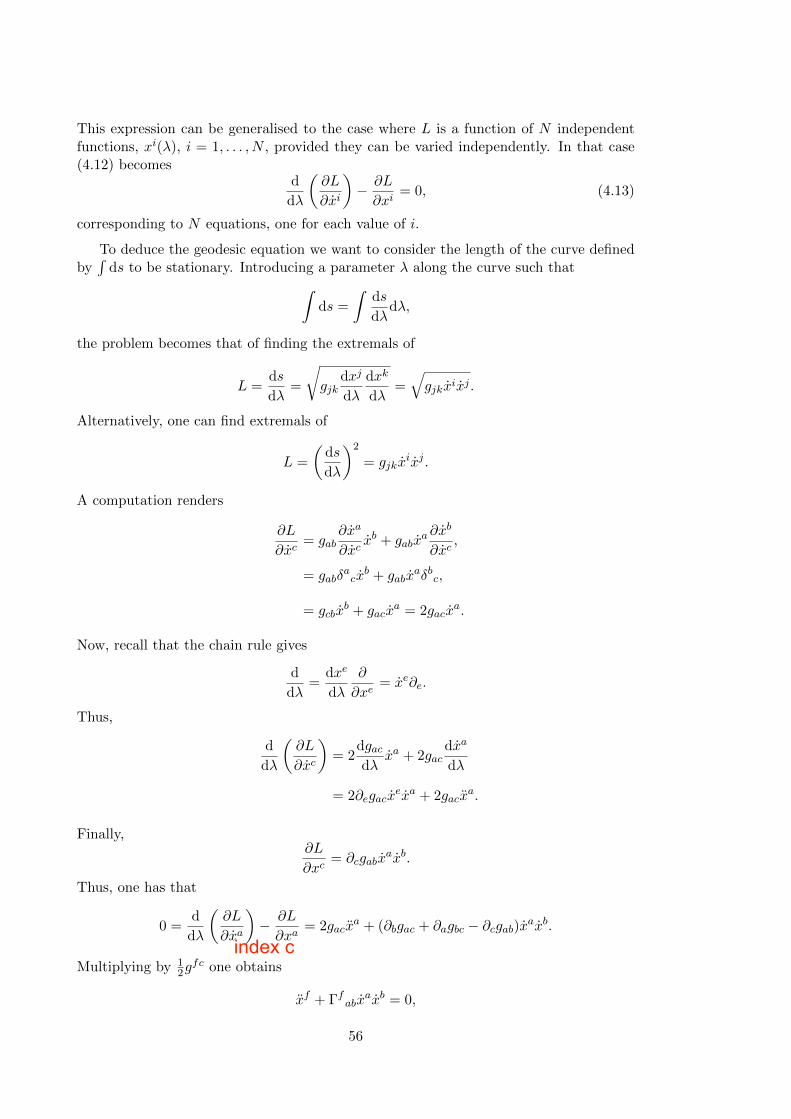
This expression can be generalised to the case where L is a function of N independentfunctions, xi(�), i = 1, . . . , N , provided they can be varied independently. In that case(4.12) becomes
d
d�
✓@L
@xi
◆� @L
@xi= 0, (4.13)
corresponding to N equations, one for each value of i.
To deduce the geodesic equation we want to consider the length of the curve definedbyRds to be stationary. Introducing a parameter � along the curve such that
Zds =
Zds
d�d�,
the problem becomes that of finding the extremals of
L =ds
d�=
rgjk
dxj
d�
dxk
d�=qgjkxixj .
Alternatively, one can find extremals of
L =
✓ds
d�
◆2
= gjkxixj .
A computation renders
@L
@xc= gab
@xa
@xcxb + gabx
a@xb
@xc,
= gab�acx
b + gabxa�bc,
= gcbxb + gacx
a = 2gacxa.
Now, recall that the chain rule gives
d
d�=
dxe
d�
@
@xe= xe@e.
Thus,
d
d�
✓@L
@xc
◆= 2
dgacd�
xa + 2gacdxa
d�
= 2@egacxexa + 2gacx
a.
Finally,@L
@xc= @cgabx
axb.
Thus, one has that
0 =d
d�
✓@L
@xa
◆� @L
@xa= 2gacx
a + (@bgac + @agbc � @cgab)xaxb.
Multiplying by 12g
fc one obtains
xf + �fabx
axb = 0,
56
index c
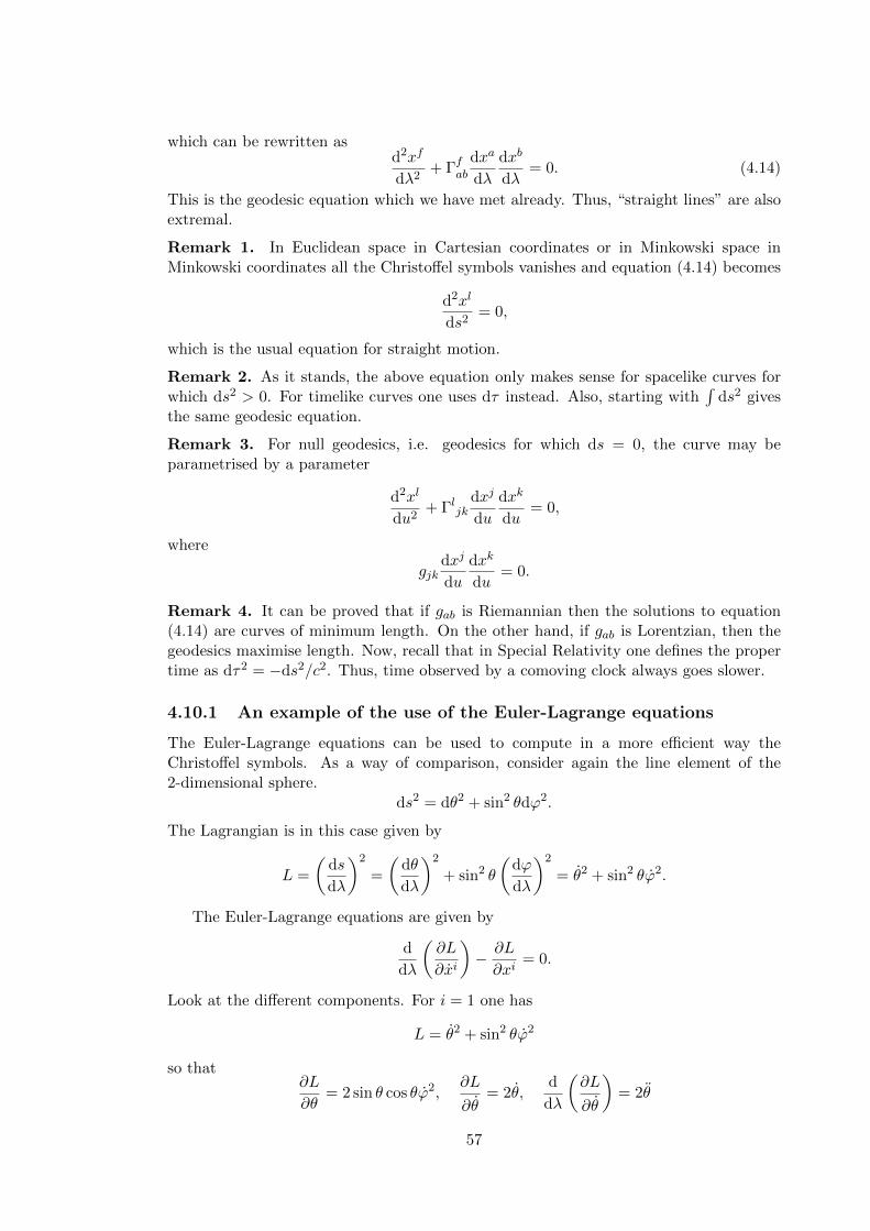
which can be rewritten asd2xf
d�2+ �f
ab
dxa
d�
dxb
d�= 0. (4.14)
This is the geodesic equation which we have met already. Thus, “straight lines” are alsoextremal.
Remark 1. In Euclidean space in Cartesian coordinates or in Minkowski space inMinkowski coordinates all the Christo↵el symbols vanishes and equation (4.14) becomes
d2xl
ds2= 0,
which is the usual equation for straight motion.
Remark 2. As it stands, the above equation only makes sense for spacelike curves forwhich ds2 > 0. For timelike curves one uses d⌧ instead. Also, starting with
Rds2 gives
the same geodesic equation.
Remark 3. For null geodesics, i.e. geodesics for which ds = 0, the curve may beparametrised by a parameter
d2xl
du2+ �l
jkdxj
du
dxk
du= 0,
where
gjkdxj
du
dxk
du= 0.
Remark 4. It can be proved that if gab is Riemannian then the solutions to equation(4.14) are curves of minimum length. On the other hand, if gab is Lorentzian, then thegeodesics maximise length. Now, recall that in Special Relativity one defines the propertime as d⌧2 = �ds2/c2. Thus, time observed by a comoving clock always goes slower.
4.10.1 An example of the use of the Euler-Lagrange equations
The Euler-Lagrange equations can be used to compute in a more e�cient way theChristo↵el symbols. As a way of comparison, consider again the line element of the2-dimensional sphere.
ds2 = d✓2 + sin2 ✓d'2.
The Lagrangian is in this case given by
L =
✓ds
d�
◆2
=
✓d✓
d�
◆2
+ sin2 ✓
✓d'
d�
◆2
= ✓2 + sin2 ✓'2.
The Euler-Lagrange equations are given by
d
d�
✓@L
@xi
◆� @L
@xi= 0.
Look at the di↵erent components. For i = 1 one has
L = ✓2 + sin2 ✓'2
so that@L
@✓= 2 sin ✓ cos ✓'2,
@L
@✓= 2✓,
d
d�
✓@L
@✓
◆= 2✓
57
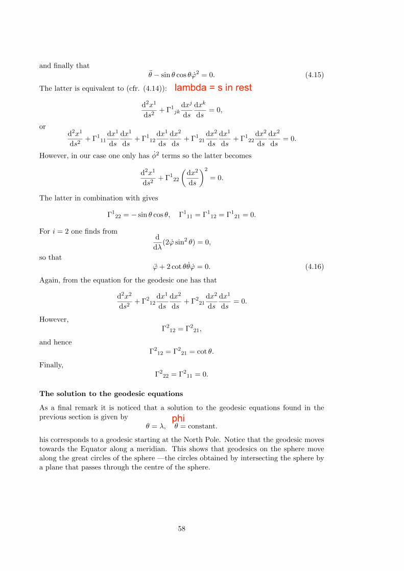
and finally that✓ � sin ✓ cos ✓'2 = 0. (4.15)
The latter is equivalent to (cfr. (4.14)):
d2x1
ds2+ �1
jkdxj
ds
dxk
ds= 0,
ord2x1
ds2+ �1
11dx1
ds
dx1
ds+ �1
12dx1
ds
dx2
ds+ �1
21dx2
ds
dx1
ds+ �1
22dx2
ds
dx2
ds= 0.
However, in our case one only has �2 terms so the latter becomes
d2x1
ds2+ �1
22
✓dx2
ds
◆2
= 0.
The latter in combination with gives
�122 = � sin ✓ cos ✓, �1
11 = �112 = �1
21 = 0.
For i = 2 one finds fromd
d�(2' sin2 ✓) = 0,
so that'+ 2 cot ✓✓' = 0. (4.16)
Again, from the equation for the geodesic one has that
d2x2
ds2+ �2
12dx1
ds
dx2
ds+ �2
21dx2
ds
dx1
ds= 0.
However,�2
12 = �221,
and hence�2
12 = �221 = cot ✓.
Finally,�2
22 = �211 = 0.
The solution to the geodesic equations
As a final remark it is noticed that a solution to the geodesic equations found in theprevious section is given by
✓ = �, ✓ = constant.
his corresponds to a geodesic starting at the North Pole. Notice that the geodesic movestowards the Equator along a meridian. This shows that geodesics on the sphere movealong the great circles of the sphere —the circles obtained by intersecting the sphere bya plane that passes through the centre of the sphere.
58
lambda = s in rest
phi
Chapter 5
Curvature
A novel feature of General Relativity is that it employs the notion of curved space. Ourintuition of curvature is mainly based on the curvature of 2-dimensional objects in 3-dimensional space, like spheres, saddles, etc. The notion of curvature whose definitiondepends on a space of higher dimension is called extrinsic. In the case of spacetime thisnotion is not useful and require an intrinsic notion —i.e. a definition which is independentof the embedding space.
5.1 Intrinsic curvature and the Riemann tensor
Gauss showed that for a general 2-dimensional surface with a metric of the form
ds2 = g11(x1, x2)(dx1)2 + g22(x
1, x2)(dx2)2,
where it has been assumed that g12 = 0 for simplicity, it is possible to define an intrinsiccurvature (a scalar function) which is invariant under coordinate transformations, butvaries from point to point. This is given by an expression of the form
K = F [gij , @kgij , @l@kgij ],
such that when K = 0 the space is flat and for a sphere of radius R it gives K = 1/R2.
In spaces of higher dimension we require more than one quantity at each point todescribe curvature. It turns out that the right definition involves the components of a4-index tensor called the Riemann curvature tensor :
Rabcd ⌘ @c�
abd � @d�
abc + �a
ec�ebd � �a
ed�ebc. (5.1)
Since the Christo↵el symbols contain derivatives of the metric, one finds that the Riemanntensor has the same form as K. Note that in flat space given by Cartesian coordinatesthe Christo↵el symbols vanish, and thus the Riemann tensor vanishes! If one showsthat Ra
bcd is indeed a tensor, then this last statement is valid for any coordinates! Thisstatement is actually an if and only if statement. The hard part is to show that vanishingcurvature implies Minkowski space.
There are many ways of motivating this formula. Here we will proceed by looking atthe commutation of covariant derivatives. Consider:
rcrbVa �rbrcVa = Va;b;c � Va;c;b.
59
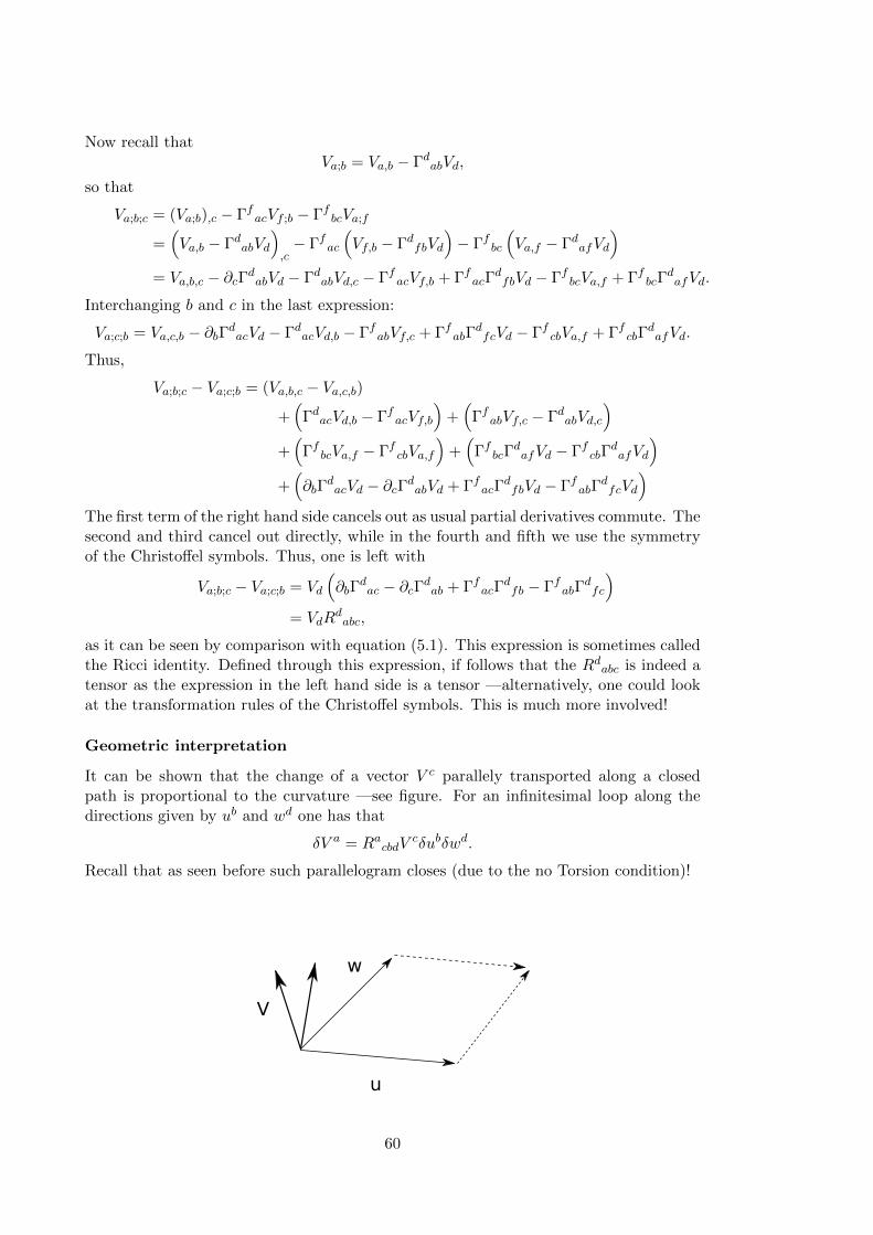
Now recall thatVa;b = Va,b � �d
abVd,
so that
Va;b;c = (Va;b),c � �facVf ;b � �f
bcVa;f
=⇣Va,b � �d
abVd
⌘
,c� �f
ac
⇣Vf,b � �d
fbVd
⌘� �f
bc
⇣Va,f � �d
afVd
⌘
= Va,b,c � @c�dabVd � �d
abVd,c � �facVf,b + �f
ac�dfbVd � �f
bcVa,f + �fbc�
dafVd.
Interchanging b and c in the last expression:
Va;c;b = Va,c,b � @b�dacVd � �d
acVd,b � �fabVf,c + �f
ab�dfcVd � �f
cbVa,f + �fcb�
dafVd.
Thus,
Va;b;c � Va;c;b = (Va,b,c � Va,c,b)
+⇣�d
acVd,b � �facVf,b
⌘+⇣�f
abVf,c � �dabVd,c
⌘
+⇣�f
bcVa,f � �fcbVa,f
⌘+⇣�f
bc�dafVd � �f
cb�dafVd
⌘
+⇣@b�
dacVd � @c�
dabVd + �f
ac�dfbVd � �f
ab�dfcVd
⌘
The first term of the right hand side cancels out as usual partial derivatives commute. Thesecond and third cancel out directly, while in the fourth and fifth we use the symmetryof the Christo↵el symbols. Thus, one is left with
Va;b;c � Va;c;b = Vd
⇣@b�
dac � @c�
dab + �f
ac�dfb � �f
ab�dfc
⌘
= VdRdabc,
as it can be seen by comparison with equation (5.1). This expression is sometimes calledthe Ricci identity. Defined through this expression, if follows that the Rd
abc is indeed atensor as the expression in the left hand side is a tensor —alternatively, one could lookat the transformation rules of the Christo↵el symbols. This is much more involved!
Geometric interpretation
It can be shown that the change of a vector V c parallely transported along a closedpath is proportional to the curvature —see figure. For an infinitesimal loop along thedirections given by ub and wd one has that
�V a = RacbdV
c�ub�wd.
Recall that as seen before such parallelogram closes (due to the no Torsion condition)!
�
�
�
60
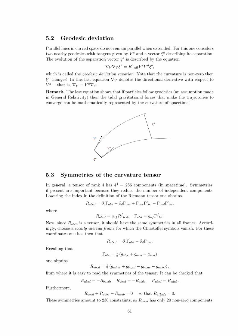
5.2 Geodesic deviation
Parallel lines in curved space do not remain parallel when extended. For this one considerstwo nearby geodesics with tangent given by V a and a vector ⇠a describing its separation.The evolution of the separation vector ⇠a is described by the equation
rV rV ⇠a = Ra
cdbVcV d⇠b,
which is called the geodesic deviation equation. Note that the curvature is non-zero then⇠a changes! In this last equation rV denotes the directional derivative with respect toV a —that is, rV ⌘ V ara.
Remark. The last equation shows that if particles follow geodesics (an assumption madein General Relativity) then the tidal gravitational forces that make the trajectories toconverge can be mathematically represented by the curvature of spacetime!
5.3 Symmetries of the curvature tensor
In general, a tensor of rank 4 has 44 = 256 components (in spacetime). Symmetries,if present are important because they reduce the number of independent components.Lowering the index in the definition of the Riemann tensor one obtains
Rabcd = @c�abd � @d�abc + �aec�ebd � �aed�
ebc,
whereRabcd = gafR
fbcd, �abd = gaf�
fbd.
Now, since Rabcd is a tensor, it should have the same symmetries in all frames. Accord-ingly, choose a locally inertial frame for which the Christo↵el symbols vanish. For thesecoordinates one has then that
Rabcd = @c�abd � @d�abc.
Recalling that�abc =
12 (gab,c + gac,b � gbc,a)
one obtainsRabcd = 1
2 (gad,bc + gbc,ad � gbd,ac � gac,bd) ,
from where it is easy to read the symmetries of the tensor. It can be checked that
Rabcd = �Rbacd, Rabcd = �Rabdc, Rabcd = Rcdab.
Furthermore,Rabcd +Radbc +Racdb = 0 so that Ra(bcd) = 0.
These symmetries amount to 236 constraints, so Rabcd has only 20 non-zero components.
61
5.4 Bianchi identities, the Ricci and Einstein tensors
Recall that in a locally inertial frame one had that
Rabcd = 12(gbc,ad + gad,bc � gbd,ac � gac,bd).
Di↵erentiating with respect to xe one obtains
Rabcd,e =12(gbc,ade + gad,bce � gbd,ace � gac,bde).
Using the fact that partial derivatives commute one finds that
Rabcd,e +Rabec,d +Rabde,c = 0, Rab(cd,e) = 0.
Now, in a locally inertial frame the Christo↵el symbols vanish so that in fact one hasthat
Rabcd;e +Rabec;d +Rabde;c = 0, Rab(cd;e) = 0.
This tensorial equation is valid in all frames and is called the Bianchi identity. One couldhave derived it by directly taking the covariant derivative of the Riemann tensor.
The Ricci tensor
The Ricci tensor is obtained by contracting the first and third indices of the Riemanntensor:
Rbd ⌘ gacRabcd = Rcbcd.
Remark 1. Because of the symmetries of the Riemann tensor one has that the Riccitensor is symmetric. That is,
Rbd = Rdb.
Remark 2. Other contractions of the Riemann tensor vanish or give ±Rbd. For exampleRb
bcd = 0 since Rabcd is symmetric on a and b. Also,
Rabda = �Ra
bad = �Rbd,
and similarly.
The Ricci scalar
The Ricci scalar is defined as the contraction of the indices of the Ricci tensor:
R ⌘ gabRab = gacgbdRabcd.
The Einstein tensor
In the next computations recall that gab;c = 0 and gab;c = 0. Consider the Bianchiidentity, contract with gac and bringing gac into the covariant derivative:
(gacRabcd);e + (gacRabec);d + (gacRabde);c = 0. (5.2)
Now,gacRabcd = Rbd, gacRabec = �gacRabce,
62
[ ] not ( )
[ ] not ( )
so that (5.2) rendersRbd;e �Rbe;d +Rc
bde;c = 0.
Contracting on b and d:R;e �Rd
e;d �Rce;c = 0, (5.3)
where it has been used that
gbdRcbde = gbdgcaRabde = �gcagbdRbade = �gcaRae = �Rc
e.
On can rewrite equation (5.3) as
(2Rce � �ceR);c = 0. (5.4)
Raising e one gets(2Rcd � gcdR);c = 0.
DefiningGcd ⌘ Rcd � 1
2Rgcd
one hasGcd
;c = 0.
The tensor Gcd is called the Einstein tensor. Observe that one can also lower the indices:
Gfe = Rfe � 12Rgfe.
Remark 1. The Einstein tensor is symmetric (from the symmetries of the Ricci andmetric tensors) and therefore it has 10 independent components.
Remark 2. By construction, the Einstein tensor is divergence free.
63
e

64
Chapter 6
General Relativity
6.1 Towards the Einstein equations
There are several ways of motivating the Einstein equations. The most natural is perhapsthrough considerations involving the Equivalence Principle. In gravitational fields thereexist local inertial frames in which Special Relativity is recovered. The equation of motionof a free particle in such frames is:
d2x0a
d⌧2= 0.
Relative to an arbitrary (accelerating frame) specified by xa = xa(x0b), the latter becomes:
d2xa
d⌧2+ �abc
dxb
d⌧
dxc
d⌧= 0,
where
�abc =@xa
@x0d@2x0d
@xb@xc.
Here the �abc are the “fictitious” terms that arise due to the non-inertial nature of theframe.
Now, due to the Equivalence Principle the latter implies that locally gravity is equiv-alent to acceleration and this in turn gives rise to non-inertial frames. The main idea ofGeneral relativity is to argue that gravitation as well as inertial forces should be describedby appropriate �abc’s!
The simplest way to do this is by means of a Lorentzian manifold —the latter isendowed with geodesics of the required type:
d2xa
d⌧2+ �a
bcdxb
d⌧
dxc
d⌧= 0.
Now, if the �a0bcs are associated with gravitational forces, then the metric gab may be
associated with a potential. Note that the gravitational potential in the Newtoniantheory satisfies
r2� = 4⇡G⇢, ⇢ the density.
The relativistic analogue of this equation should be tensorial and of second order in themetric. To take this analogy further, consider two neighbouring particles with coordinates
65
x↵(t), x↵(t) + ⇠↵(t), with ⇠↵(t) small ↵ = 1, 2, 3, moving in a gravitational field with apotential �. the equations of motion are then given:
x↵ = �@�(x)
@x↵
and
x↵ + ⇠↵ = �@�(x)
@x↵� ⇠�
@2�
@x↵@x�+O(⇠2).
Subtracting the two last equations:
⇠ = �⇠�@2�
@x↵@x�.
This is the relative acceleration of two test particles separated by by a 3-vector ⇠↵ —thesecond derivative of the potential gives the tidal forces. This is in analogy to the geodesicdeviation equation:
rV rV ⇠↵ = Ra
cdbVcV d⇠b,
provided that one identifies
�⇠�@2�
@x↵@x�, and Ra
cdbVcV d⇠b.
This identification would make clear the relation between gravity and geometry —notethat the Riemann tensor involves second derivatives of the metric tensor.
6.2 Principles employed in General Relativity
The main idea underlying General Relativity is that matter–including energy–curvesspacetime (assumed to be a Lorentzian manifold). This in turn a↵ects the motion ofparticles and light rays, postulated to move on timelike and null geodesics of the manifold,respectively. These ideas are understood in conjunction with the main principles ofGeneral Relativity, listed below.
(1) Equivalence Principle.
(2) Principle of General Covariance. This states that laws of Nature should havetensorial form.
(3) Principle of minimal gravitational coupling. This is used to derive the Gen-eral Relativity analogues of Special Relativity results. For this change
⌘ab ! gab, @ ! r.
For example in Special Relativity the equations for a perfect fluid are given by:
T ab = (⇢+ p)V aV b � p⌘ab,
T ab,b = 0.
In General Relativity these should be changed to:
T ab = (⇢+ p)V aV b � pgab,
T ab;b = 0.
(4) Correspondence principle. General relativity must agree with Special Relativityin absence of gravitation and with Newtonian gravitational theory in the case ofweak gravitational fields and in the non-relativistic limit (slow speed).
66
a
alpha index on xi
6.2.1 The Einstein equations in vacuum
In vacuum, such as in the outside of a body in empty space, one has that the density ⇢vanishes and the equation for the Newtonian potential becomes:
r2� = 0.
The Laplace equation involves an object with two indices (@2�/@xi@xj). As a result,what one needs is an object with two indices —a contraction of the Riemann tensor, likethe Ricci tensor:
Rbc = 0. (6.1)
The latter are called the Einstein vacuum field equations. The vacuum equations forma set of ten nonlinear, second order partial di↵erential equations for the components ofthe metric tensor gab. These are hard to solve, apart from simple settings.
Remark 1. One of the simplest solutions to the vacuum equations is Minkowski space-time. Expressing the metric ⌘ab locally as ds2 = �dt2 + dx2 + dy2 + dz2, we see that allthe Christo↵el symbols vanish, from which Rab = 0 is trivially satisfied.
Remark 2. The most general form of the vacuum equations which is tensorial anddepends linearly on second derivatives of the metric is:
Rbc = ⇤gab,
where ⇤ is the so-called Cosmological constant. Outside Cosmology, ⇤ is usually takento be zero.
6.2.2 The (full) Einstein Equations
Matter in relativity is described by a (0,2) tensor Tab called the energy-momentum tensor.Conservation of mass-energy is described by raTab = 0, consistent with the calculationdone in the Special Relativity case. Equating Tab with a curvature tensor with vanishingdivergence, one has
Gab = Tab.
Note, however, that since ragab = 0, we could also have written
Gab + ⇤gab = Tab. (6.2)
These are the complete Einstein field equations for the metric gab of a spacetime.Note that the Einstein equations are the simplest compatible with the Equivalence
Principle, but they are not the only ones. In general, the Einstein field equations areextremely complicated set of non-linear partial di↵erential equations. In some simplesettings, analytic solutions may be found. These include:
(i) The vacuum spherically symmetric static case (the Schwarzschild spacetime).
(ii) The weak field case (gravitational waves).
(iii) The isotropic and homogeneous case (Cosmology).
We will discuss the first case now.
67
6.3 The Schwarzschild solution
This is the basis for nearly all the tests of General Relativity. The solution correspondsto the metric corresponding to a static, spherically symmetric gravitational field in theempty spacetime surrounding a central mass (like the Sun).
Choosing coordinates (t, r, ✓,'), it can be shown that a metric of this type is of theform:
ds2 = �eA(r)dt2 + eB(r)dr2 + r2(d✓2 + sin2 ✓d'2), (6.3)
where A(r) and B(r) describe deviation of the metric from Minkowski spacetime. Notethat for constant t and r the metric reduces to the standard metric for the surface of asphere. As one is dealing with vacuum, one is poised to solve
Rab = 0. (6.4)
Substituting (6.3) in (6.4), and after some algebra, the only non-zero components of (6.4)have the form:
Rrr = R11 =12A
00 � 14A
0B0 + 14A
02 � B0
r, , (6.5a)
R✓✓ = R22 = e�B�1 + 1
2r(A0 �B0)
�� 1, , (6.5b)
R'' = R33 = R22 sin2 ✓, (6.5c)
Rtt = R00 = �eA�B
✓12A
00 � 14A
0B0 + 14A
02 +A0
r
◆, (6.5d)
where 0 denotes di↵erentiation with respect to r.
To solve Rab = 0, we start by looking at the combination:
Rrr + eB�ARtt = � 12r (B
0 +A0) = 0.
Integrating one obtainsA = �B.
One can without loss of generality change t to absorb the constant of integration. Sub-stituting in (6.5b):
eA(1 + rA0)� 1 = 0.
The latter can be rewritten as(reA)0 = 1,
which can be integrated to give
reA = r + �, � a constant
so thateA = 1 +
�
r,
so that the metric one obtains is given by
ds2 = �⇣1 +
�
r
⌘dt2 +
⇣1 +
�
r
⌘�1dr2 + r2(d✓2 + sin2 ✓d'2).
To fix �, we use the fact that in the Newtonian limit of a central mass M ,
g00 = �✓1� 2GM
r
◆.
68
We shall prove this statement in the next subsection. Next, comparing with
�⇣1 +
�
r
⌘,
one finds that� = �2GM.
Hence, at the end of the day one has
ds2 = �✓1� 2GM
r
◆dt2 +
✓1� 2GM
r
◆�1
dr2 + r2(d✓2 + sin2 ✓d'2). (6.6)
The latter is called the Schwarzschild metric.
Remark 1. This solution demonstrates how the presence of mass curves flat spacetime.
Remark 2. The metric (6.6) is asymptotically flat. That is, it becomes Minkowskian asr ! 1.
Remark 3. The solution only applies to the exterior of a star.
Remark 4. The Birkho↵ Theorem: a spherically symmetric solution in vacuum isnecessarily static. That is, there is no time dependence is spherically symmetric solutions.
6.3.1 Newtonian limit
In this subsection, we return to the statement above which fixed the value of � by usingthe Newtonian limit of a central mass M via g00 = �
�1� 2GM
r
�.
Consider a slowly moving particle in a weak stationary gravitational field. Recall thegeodesic equation:
d2xa
d⌧2+ �a
bcdxb
d⌧
dxc
d⌧= 0. (6.7)
For a slow moving particle dx↵/d⌧ (↵ = 1, 2, 3) may be neglected relative to dt/d⌧ , sothat (6.7) implies that
d2xa
d⌧2+ �a
00
✓dt
d⌧
◆2
= 0. (6.8)
Since the gravitational field is assumed to be stationary, all t-derivatives of gab vanishand therefore
�a00 = �1
2gad@g00
@xd. (6.9)
Furthermore, since the field is weak, one may adopt a local coordinate system in which
gab = ⌘ab + hab, |hab| ⌧ 1. (6.10)
Substitution into (6.9) one has that
�a00 = �1
2⌘ad@h00
@xd.
Substituting in (6.8):
d2x↵
d⌧2= 1
2
✓dt
d⌧
◆2
rh00, r ⌘ ⌘↵�@
@x�, (6.11a)
d2t
d⌧2= 0, as h00,0 = 0. (6.11b)
69
alpha index on nablas
From (6.11a) it follows that dt/d⌧ is a constant. Also, from
dx↵
d⌧=
dx↵
dt
dt
d⌧,
it follows thatd2x↵
d⌧2=
d2x↵
dt2
✓dt
d⌧
◆2
+dx↵
dt
d2t
d⌧2,
which in our case reduces to
d2x↵
d⌧2=
d2x↵
dt2
✓dt
d⌧
◆2
.
Combining the latter with (6.11a)
d2x↵
dt= 1
2rh00. (6.12)
The corresponding Newtonian result is
d2x↵
dt= �r� (6.13)
where � is the gravitational potential which far from a central body of mass M at adistance r is given by
� = �GM
r.
Comparing (6.12) and (6.13) one finds then that
h00 = �2�+ constant.
However, at large distances from M one has that � ! 0 (gravity becomes negligible) andgab ! ⌘ab (the space becomes flat). Therefore the constant must be zero so that
h00 = �2�.
Substituting in (6.10) on findsg00 = �(1 + 2�).
Now, recall that � has dimensions of (velocity)2, [�] = [GM/R] = L2/T 2. Therefore onehas that �/c2 at the surface of the Earth is ⇠ 10�9, one the surface of the Sun ⇠ 10�6
and at the surface of a white dwarf ⇠ 10�4. It follows that in most cases the distortionproduced by gravity is in gab very small.
70
- is
-
6.4 Applications and Experimental Tests of GR
The classical experimental tests of General Relativity are based on the Schwarzschildsolution. These are based on the comparison of the trajectories of freely falling particlesand light rays in gravitational field of a central body with their counterparts in Newtoniantheory.
In order to derive the geodesics in Schwarzschild spacetime, it is best to use theEuler-Lagrange equations with
L =
✓d⌧
d�
◆2
=
✓1� 2MG
r
◆t2 �
✓1� 2MG
r
◆�1
r2 � r2(✓2 + sin2 ✓'2),
where 0 denotes di↵erentiation with respect to the parameter �. For timelike geodesicsone has that � = ⌧ so that L = 1. On the other hand, for null geodesics L = 0.
The Euler-Lagrange equations read then
d
d�
�2At
�= 0, , (6.14a)
d
d�(2rA�1)� 2r(✓2 + sin2 ✓'2) + r2A�2A0 + t2A0 = 0, (6.14b)
d
d�(r2✓)� r2 sin ✓ cos ✓'2 = 0, (6.14c)
d
d�(r2 sin2 ✓') = 0, (6.14d)
where
A(r) =
✓1� 2GM
r
◆,
and 0 denotes di↵erentiation with respect to r. It turns out that it is simpler to use
✓1� 2MG
r
◆t2 �
✓1� 2MG
r
◆�1
r2 � r2(✓2 + sin2 ✓'2) = 1, 0. (6.15)
This is, in fact, an integral of motion of the Euler-Lagrange equation. It expresses thefact that the square of the norm of the 4-velocity vector of a timelike particle is �1, whilethat of a photon is 0. This is like in Special Relativity.
As in Classical Mechanics (central force orbit), let us look for solutions in the Equa-torial plane: ✓ = ⇡/2. It follows then that ✓ = 0, and from (6.14c) with cos ✓ = 0one finds that ✓ = 0. The orbits remain in a plane! This is like in Classical Mechanics—conservation of angular momentum.
Now, from (6.14d) it follows that
r2' = h, h a constant, (6.16a)✓1� 2GM
r
◆t = l, l a constant, . (6.16b)
Substituting (6.16a) and (6.16b) in (6.15) one obtains
l2✓1� 2GM
r
◆�1
�✓1� 2GM
r
◆�1
r2 � h2
r2= 1, 0. (6.17)
71
dot
As in Newtonian theory, let u = 1/r so that
r =dr
d�=
dr
d'
d'
d�= '
dr
d',
dr
d'= � 1
u2du
d'.
Using (6.16a) one finds
r = �hdu
d'.
Then equation (6.17) in (u,') coordinates become
✓du
d'
◆2
+ u2 =l2 � 1
h2+
2GM
h2u+
2GMu3
c2, for timelike geodesics, (6.18a)
✓du
d'
◆2
+ u2 =l2
h2+
2GMu3
c2, for null geodesics. (6.18b)
The speed of light c has been added for dimensional reasons. These are the analoguesof energy equations in Newtonian theory. One can solve (6.19a)-(6.19b) approximately.For this, di↵erentiate the equations with respect to ':
d2u
d'2+ u =
GM
h2+
3GMu2
c2, for timelike geodesics, (6.19a)
d2u
d'2+ u =
3GMu2
c2, for null geodesics. (6.19b)
From here, one has to analyse the two cases separately.
6.4.1 The photon sphere
As a first application of the geodesic equations in the Schwarzschild spacetime, it willbe shown that there exist a certain sphere (of radius to be determined) on which rays oflight move in circular orbits!
As in the previous discussion we consider light moving on the Equatorial plane —notice that this can be assumed without loss of generality due to the spherical symmetry.Any results obtained from the analysis of motion on the Equatorial plane holds for anyother plane. It follows that ✓ = 0, ✓ = ⇡/2. In what follows we will consider circularorbits —thus, r is constant and one has r = 0. Substituting into the first integral (6.15)with the value 0 one obtains
✓1� 2Gm
r
◆t2 = r2'2.
Alternatively, one can write
✓1� 2Gm
r
◆✓dt
d�
◆2
= r2'2
✓d'
d�
◆2
.
It follows then that ✓d'
dt
◆2
=1
r2
✓1� 2Gm
r
◆. (6.20)
Now, using equation (6.14b) and substituting again ✓ = ⇡/2, ✓ = 0, r = 0 on obtains
A0t2 = 2r'2.
72
change to caps M in this section
x
M
A computation shows that
A0 =2Gm
r2,
and hence one obtainsGm
r3
✓dt
d�
◆2
=
✓d'
d�
◆2
.
It follows that ✓d'
dt
◆2
=Gm
r3. (6.21)
Equating expressions (6.20) and (6.21) one obtains
1
r2
✓1� 2Gm
r
◆=
Gm
r3,
from where one can deduce thatr = 3Gm.
This is the radius indicating the locating of the photon sphere —the surface on whichrays of light orbit in circular orbits.
6.4.2 Timelike case —an orbiting particle
The appropriate equation (6.19a) is identical to the equation for Newtonian orbits exceptfor the last term. This last term is small relative to other terms for planetary orbits. Theration of the last two terms for Mercury is ⇠ 10�7. As a consequence of this, equation(6.19a) will be solved using perturbation methods. For this let
a ⌘ GM
h2, ✏ =
✓3GM
c2
◆GM
h2,
where ✏ is dimensionless and assumed to be small. Then equation (6.19a) implies
d2u
d'2+ u = a+
✏
au2. (6.22)
We will look for solutions of the type
u = u0 + ✏u1 +O(✏2).
Substitution in (6.22) yields
d2u0d'2
+ u0 + ✏
✓d2u1d'2
+ u1
◆= a+
✏
au20 +O(✏2). (6.23)
Equating zeroth order terms in ✏ in equation (6.23) one obtains
d2u0d'2
+ u0 = a,
which can be solved to give
u0 = a+ b cos', b a constant, (6.24)
73
where without loss of generality we have set '0 = 0. Now, equating the first order termin (6.23) one has
d2u1d'2
+ u1 =u20a.
Substituting for u0 from (6.24), and using that
cos2 ' = 12(1 + cos 2'),
one obtainsd2u1d'2
+ u1 =
✓a+
b2
2a
◆+ 2b cos'+
b2
2acos 2', (6.25)
which is a linear inhomogeneous ordinary di↵erential equation. Its general solution con-sists of a general solution to the homogeneous part plus a particular solution correspond-ing to each term of the right hand side of (6.25). One has that for:
a+b2
2a, the solution is a+
b2
2a,
2b cos' the solution is b' sin',
b2
2acos 2' the solution is � b2
6acos 2'.
Hence, the solution to the orbit equation to first order in ✏ is
u = u0 + ✏u1
=
✓a+ ✏a+
b2
2a✏
◆+
✓b cos'� b2
6a✏ cos 2'
◆+ ✏b' sin'.
It is observed that only the last term in this expression is non-periodic, and hence, anyirregularity in the orbit (non-periodicity) must relate to this term. To see the e↵ect ofthis term recall that
cos ✏' ⇡ 1, sin ✏' ⇡ ✏',
so that
cos('� ✏') = cos' cos ✏'+ sin' sin ✏' = cos'+ ✏' sin'.
Hence, we write the solution as
u = a+ b cos('� ✏') + ✏
✓a+
b2
2a� b2
6acos 2'
◆,
that is:
u = a+ b cos('� ✏') + (periodic terms).
New, recall that the perihelion of a planet around the Sun occurs when r is a minimum(u maximum). Now, cos('� ✏') is a maximum when
'(1� ✏) = 2n⇡, or approximately ' ⇡ 2n⇡(1 + ✏).
Successive perihelia occur then at intervals of
�' ⇡ 2⇡(1 + ✏),
74
instead of 2⇡ as in the case of periodic motion. Therefore, the perihelion shift perrevolution (�' = �'� 2⇡) is
�' = 2⇡✏ =6⇡G2M2
h2c2.
From Newtonian theory we have that
↵ =h2
GM(1� e2), T 2 =
4⇡2↵3
GM,
where e is the eccentricity of the orbit, ↵ the semi-major axis, and T the period. Oneobtains then that
�' =24⇡3↵2
c2T 2(1� e2).
For the case of the planet Mercury this gives a total shift of 43.0300 per century which isin good agreement with the classically unaccounted shift of 43.1100 ± 0.4500.
Remark 1. This is one of the famous classical tests of General Relativity, the so-calledperihelium shift of Mercury.
Remark 2. The e↵ect is largest in Mercury because of its high eccentricity and smallperiod which results in a large shift.
Remark 3. For Venus one has a predicted shift of 8.600 and an observed of 8.400 ± 4.800.For the Earth one has 3.800 and 5.000± 1.200. For the asteroid Icarus 10.300 and 9.800± 0.800.
6.4.3 Null geodesics
The relevant equation for null geodesics is given by (6.19b):
d2u
d'2+ u =
3GMu2
c2.
As before, the term GMu/c2 is small relative to u so let ✏ ⌘ 3GM/c2, and rewrite (6.19b)as
d2u
d'2+ u = ✏u2, . (6.26)
As before, look for solutions of the form
u = u0 + ✏u1 +O(✏2).
Substituting into (6.26) one has
d2u0d'2
+ u0 + ✏d2u1d'2
+ ✏u1 = ✏u20 +O(✏2).
Equation the zero terms in the previous equation:
d2u0d'2
+ u0 = 0,
which can be solved to give
u0 = L cos', L a constant.
75

Now, u0 = 1/r so that
r cos' =1
L,
which represents a straight line —which is what is expected. To zeroth order light is notdeflected by the gravitational field of the Sun.
���
Equating terms of order one in ✏ one obtains
d2u1d'2
+ u1 = u20 = L2 cos2 ' = 12L
2(1 + cos2')
which has the particular solution
u1 =12L
2 � 16L
2 cos 2' = 23L
2 � 13L
2 cos2 '.
Hence, one obtains that
u = u0 + ✏u1 = L cos'+ 23L
2 � 13L
2 cos2 '. (6.27)
So, the e↵ects of the first order terms (the last 2 terms) is to make light deflect from astraight line.
For a light ray grazing the Sun and arriving at Earth, the asymptote of the trajectorycorresponds to values of ' for which r ! 1 —that is, u ! 0. Substituting in (??) thisgives
cos2 '� 3
✏Lcos'� 2 = 0.
The latter can be solved to give
cos' =3
2L✏
✓1±
q1 + 8
9✏2L
◆.
Choosing the negative sign to make cos' < 1 and expanding one finds
| cos'| ⇡��23✏L
�� =����2
c2GML
����⌧ 1,
which implies ' ⇡ ⇡/2. Let ' = ⇡/2 + � son that
sin � ⇡ 2GML/c2 ⇡ �.
One has that � is the angle that each asymptote makes with undeflected straight line.The angle between 2 asymptotes is
� = 2�.
76
2
-
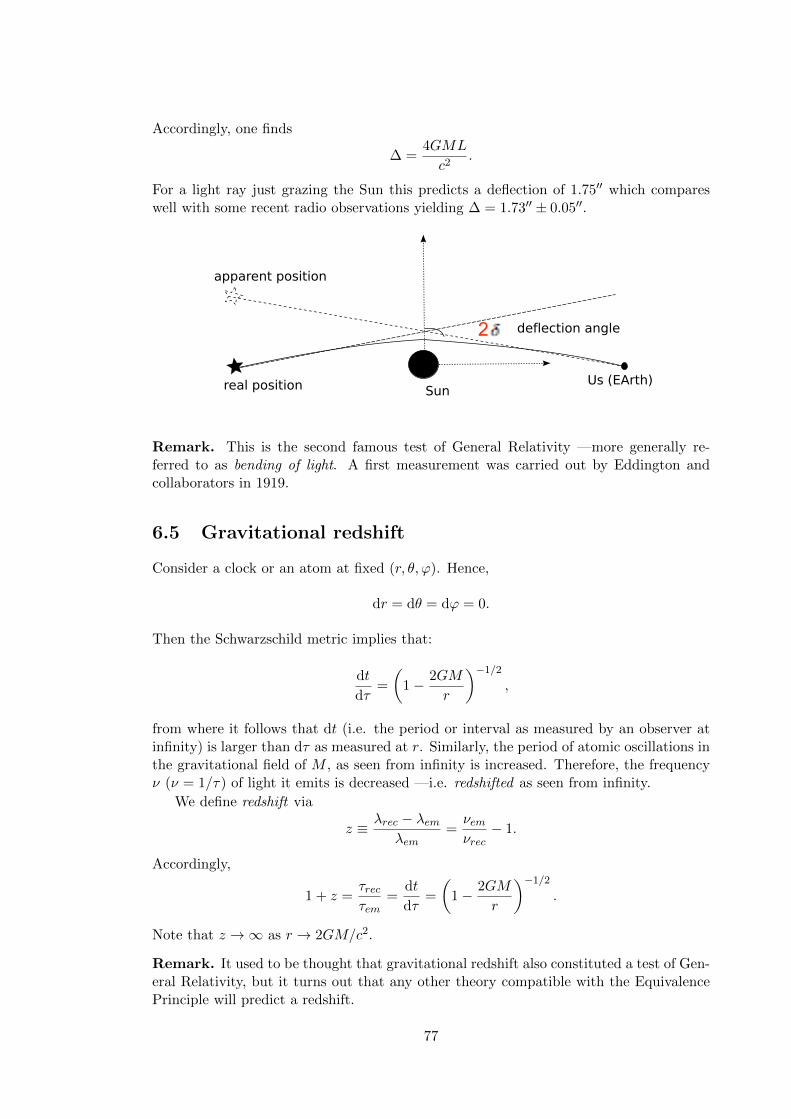
Accordingly, one finds
� =4GML
c2.
For a light ray just grazing the Sun this predicts a deflection of 1.7500 which compareswell with some recent radio observations yielding � = 1.7300 ± 0.0500.
����������
�������������
� ����������
��������������
Remark. This is the second famous test of General Relativity —more generally re-ferred to as bending of light. A first measurement was carried out by Eddington andcollaborators in 1919.
6.5 Gravitational redshift
Consider a clock or an atom at fixed (r, ✓,'). Hence,
dr = d✓ = d' = 0.
Then the Schwarzschild metric implies that:
dt
d⌧=
✓1� 2GM
r
◆�1/2
,
from where it follows that dt (i.e. the period or interval as measured by an observer atinfinity) is larger than d⌧ as measured at r. Similarly, the period of atomic oscillations inthe gravitational field of M , as seen from infinity is increased. Therefore, the frequency⌫ (⌫ = 1/⌧) of light it emits is decreased —i.e. redshifted as seen from infinity.
We define redshift via
z ⌘ �rec � �em
�em=
⌫em⌫rec
� 1.
Accordingly,
1 + z =⌧rec⌧em
=dt
d⌧=
✓1� 2GM
r
◆�1/2
.
Note that z ! 1 as r ! 2GM/c2.
Remark. It used to be thought that gravitational redshift also constituted a test of Gen-eral Relativity, but it turns out that any other theory compatible with the EquivalencePrinciple will predict a redshift.
77
2
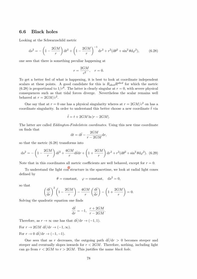
6.6 Black holes
Looking at the Schwarzschild metric
ds2 = �✓1� 2GM
r
◆dt2 +
✓1� 2GM
r
◆�1
dr2 + r2(d✓2 + sin2 ✓d'2), (6.28)
one sees that there is something peculiar happening at
r =2GM
c2, r = 0.
To get a better feel of what is happening, it is best to look at coordinate independentscalars at these points. A good candidate for this is RabcdRabcd for which the metric(6.28) is proportional to 1/r6. The latter is clearly singular at r = 0, with severe physicalconsequences such as that tidal forces diverge. Nevertheless the scalar remains wellbehaved at r = 2GM/c2.
One say that at r = 0 one has a physical singularity wheres at r = 2GM/c2 on has acoordinate singularity. In order to understand this better choose a new coordinate t via
t = t+ 2GM ln |r � 2GM |.
The latter are called Eddington-Finkelstein coordinates. Using this new time coordinateon finds that
dt = dt� 2GM
r � 2GMdr,
so that the metric (6.28) transforms into
ds2 = �✓1� 2GM
r
◆dt2 +
4GM
rdtdr+
✓1 +
2GM
r
◆dr2 + r2(d✓2 +sin2 ✓d'2). (6.29)
Note that in this coordinates all metric coe�cients are well behaved, except for r = 0.
To understand the light con structure in the spacetime, we look at radial light conesdefined by
✓ = constant, ' = constant, ds2 = 0,
so that ✓dt
dr
◆2✓1� 2GM
r
◆� 4GM
r
✓dt
dr
◆�✓1 +
2GM
r
◆= 0.
Solving the quadratic equation one finds
dt
dr= �1,
r + 2GM
r � 2GM.
Therefore, as r ! 1 one has that dt/dr ! (�1, 1).
For r ! 2GM dt/dr ! (�1,1).
For r ! 0 dt/dr ! (�1,�1).
One sees that as r decreases, the outgoing path dt/dr > 0 becomes steeper andsteeper and eventually slopes inwards for r < 2GM . Therefore, nothing, including lightcan go from r < 2GM to r > 2GM . This justifies the name black hole.
78
e
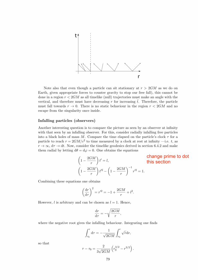
�
�
Note also that even though a particle can sit stationary at r > 2GM as we do onEarth, given appropriate forces to counter gravity to stop our free fall), this cannot bedone in a region r < 2GM as all timelike (null) trajectories must make an angle with thevertical, and therefore must have decreasing r for increasing t. Therefore, the particlemust fall towards r ! 0. There is no static behaviour in the region r < 2GM and noescape from the singularity once inside.
Infalling particles (observers)
Another interesting question is to compare the picture as seen by an observer at infinitywith that seen by an infalling observer. For this, consider radially infalling free particlesinto a black holes of mass M . Compare the time elapsed on the particle’s clock ⌧ for aparticle to reach r = 2GM/c2 to time measured by a clock at rest at infinity —i.e. t, asr ! 1, d⌧ ! dt. Now, consider the timelike geodesics derived in section 6.4.2 and makethem radial by letting d✓ = d' = 0. One obtains the equations
✓1� 2GM
r
◆t0 = l,
✓1� 2GM
r
◆t02 �
✓1� 2GM
r
◆�1
r02 = 1.
Combining these equations one obtains
✓dr
d⌧
◆2
= r02 = �1 +2GM
r+ l2.
However, l is arbitrary and can be chosen as l = 1. Hence,
dr
d⌧= �
r2GM
r,
where the negative root gives the infalling behaviour. Integrating one finds
Z ⌧
⌧0
d⌧ = � 1p2GM
Z r
r0
prdr,
so that
⌧ � ⌧0 =2
3p2GM
⇣r3/20 � r3/2
⌘.
79
change prime to dot this section
It follows that nothing special happens to this particle at r = 2GM/c2 (the Schwarzschildradius) and the body falls to r = 0 in a finite proper time ⌧ . This allows to calculate thetime taken for a large body (such a galaxy) to collapse.
Tom see what happens in coordinate time t, one can proceed from dt/dr and integrate.Alternatively, one can start with the light cones of the Schwarzschild solution (radial lightrays) given by
ds2 = 0, d✓ = d' = 0.
The Schwarzschild metric then implies
dt
dr= ± 1
1� 2GM/r,
so that as r ! 1, dt/r ! ±1, and asr ! 2GM , dt/r ! ±1.Therefore, the light cones close up as one approaches r ! 2GM . Since particles
can only move within light cones, this makes them move more and more vertically. Theapproach takes an infinite amount of t-time!
80
-