1

Andrew CLEGG

Introduction to RF Engineering

Comparing the Lingo

3

Radio Astronomers Speak a Unique Vernacular

“We are receiving interference from your transmitter at a level of 10 janskys”

“What the ^#$& is a ‘jansky’?”

4

Spectrum Managers Need to Understand a Unique Vernacular

“Huh?” “We are using +43 dBm into a 15 dBd slant-pol panel with 2 degree electrical downtilt”

5

Why Bother Learning other RF Languages?

•  Radio Astronomy is the “Leco” of RF languages, spoken by comparatively very few people

•  Successful coordination is much more likely to occur and much more easily accommodated when the parties involved understand each other’s lingo

•  It’s less likely that our spectrum management brethren will bother learning radio astronomy lingo—we need to learn theirs

6

Received Signal Strength

7

Received Signal Strength: Radio Astronomy

•  The jansky (Jy): >  1 Jy ≡ 10-26 W/m2/Hz >  The jansky is a measure of spectral power flux

density—the amount of RF energy per unit time per unit area per unit bandwidth

•  The jansky is not used outside of radio astronomy >  It is not a practical unit for measuring

communications signals §  The magnitude is much too small

>  Very few RF engineers outside of radio astronomy will know what a Jy is

8

Received Signal Strength: Communications •  The received signal strength of most

communications signals is measured in power >  The relevant bandwidth is fixed by the

bandwidth of the desired signal >  The relevant collecting area is fixed by

the frequency of the desired signal and the gain of the receiving antenna

•  Because of the wide dynamic range encountered by most radio systems, the power is usually expressed in logarithmic units of watts (dBW) or milliwatts (dBm): >  1 dBW ≡ 10log10(Power in watts) >  1 dBm ≡ 10log10(Power in milliwatts)

9

Translating Jy into dBm

•  While not comprised of the same units, we can make some reasonable assumptions to compare a Jy to dBm.

10

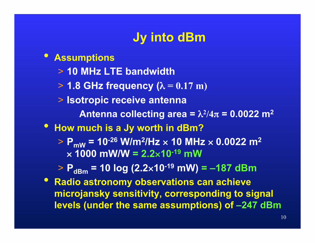
Jy into dBm •  Assumptions

>  10 MHz LTE bandwidth >  1.8 GHz frequency (λ = 0.17 m) >  Isotropic receive antenna

  Antenna collecting area = λ2/4π = 0.0022 m2

•  How much is a Jy worth in dBm? > PmW = 10-26 W/m2/Hz × 10 MHz × 0.0022 m2

× 1000 mW/W = 2.2×10-19 mW > PdBm = 10 log (2.2×10-19 mW) = –187 dBm

•  Radio astronomy observations can achieve microjansky sensitivity, corresponding to signal levels (under the same assumptions) of –247 dBm

11

Jy into dBm: Putting it into Context •  The lowest reference LTE receiver sensitivity is

–100 dBm >  minimum reported signal strength; service is

not available at this power level >  assumes 10 MHz bandwidth and QPSK

•  A 1 Jy signal strength (~-187 dBm) is therefore some 87 dB below the LTE reference receiver sensitivity

•  A µJy is a whopping 147 dB below the LTE handset reference sensitivity

A radio telescope can be more than 14 orders of magnitude more sensitive than

an LTE receiver

12

Other Units of Signal Strength: µV/m •  Received signal strengths for communications signals are

sometimes specified in units of µV/m or dB(µV/m) >  You will see µV/m used often in specifying limits on

unlicensed emissions [for example in the U.S. FCC’s Unlicensed Devices (Part 15) rules] and in service area boundary emission limits (multiple FCC rule parts)

•  This is simply a measure of the electric field amplitude (E) •  Ohm’s Law can be used to convert the electric field

amplitude into a power flux density (power per unit area): >  P(W/m2) = E2/Z0 >  Z0 ≡ (µ0/ε0)1/2 = 377 Ω = the impedance of free space

13

dBµV/m to dBm Conversion •  Under the assumption of an isotropic receiving

antenna, conversion is just a matter of algebra:

•  Which results in the following conversions:

( )

( )2MHz0

2m /s

2m/µV

21

2MHz

6

2

0

2m/µV

622

0

2V/m2

)(410

)10(4)(10

10004)W/m(1000)mW(

)(m/W

fZcE

fc

ZE

PP

ZEP

Ω=

Ω==

Ω=

−−

πππλ

m/µV10V/mdB

MHz10V/mdB

-2MHz

2m/µV

8

log20 where,log202.77)dBm(

109.1)mW(

EEfEP

fEP

=

−+−=

×= −

µ

µ

(Ohm’s law)

14

Antenna Specifications

15

Antenna Performance: Radio Astronomy

•  Radio astronomers are typically converting power flux density or spectral power flux density (both measures of power or spectral power density per unit area) into a noise-equivalent temperature

•  A common expression of radio astronomy antenna performance is the rise in system temperature attributable to the collection of power in a single polarization from a source of total flux density of 1 Jy:

•  The effective antenna collecting area Ae is a combination of the geometrical collecting area Ag (if defined) and the antenna efficiency ηa >  Ae = ηa Ag

( )K/Jy 2760102)m(

Jy

K26B2

e

KBe21

GFTkA

TkAF

≡Δ

=

Δ=⋅

−

16

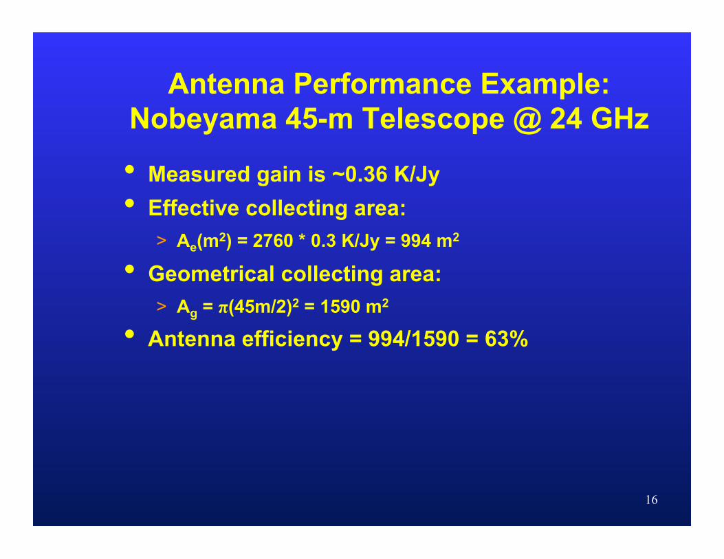
Antenna Performance Example: Nobeyama 45-m Telescope @ 24 GHz

•  Measured gain is ~0.36 K/Jy •  Effective collecting area:

>  Ae(m2) = 2760 * 0.3 K/Jy = 994 m2

•  Geometrical collecting area: >  Ag = π(45m/2)2 = 1590 m2

•  Antenna efficiency = 994/1590 = 63%

17

Antenna Performance: Communications

•  Typical communications applications specify basic antenna performance by a different expression of antenna gain: >  Antenna Gain: The amount by which the signal

strength at the output of an antenna is increased (or decreased) relative to the signal strength that would be obtained at the output of a standard reference antenna, assuming maximum gain of the reference antenna

18

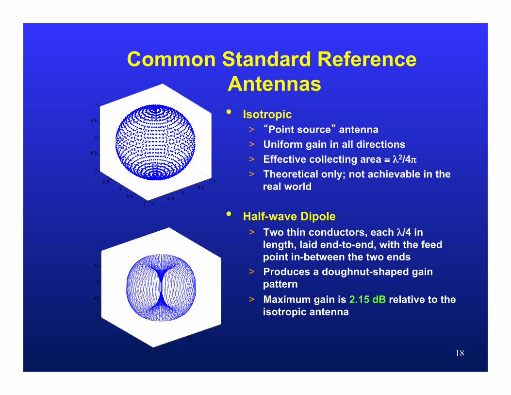
Common Standard Reference Antennas •  Isotropic

>  “Point source” antenna >  Uniform gain in all directions >  Effective collecting area ≡ λ2/4π >  Theoretical only; not achievable in the

real world

•  Half-wave Dipole >  Two thin conductors, each λ/4 in

length, laid end-to-end, with the feed point in-between the two ends

>  Produces a doughnut-shaped gain pattern

>  Maximum gain is 2.15 dB relative to the isotropic antenna

-2-1

01

2

-2-1

01

2-1

-0.5

0

0.5

1

-1-0.5

00.5

1

-1-0.5

00.5

1-1

-0.5

0

0.5

1

19

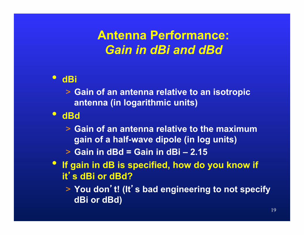
Antenna Performance: Gain in dBi and dBd

•  dBi >  Gain of an antenna relative to an isotropic

antenna (in logarithmic units) •  dBd

>  Gain of an antenna relative to the maximum gain of a half-wave dipole (in log units)

>  Gain in dBd = Gain in dBi – 2.15 •  If gain in dB is specified, how do you know if

it’s dBi or dBd? >  You don’t! (It’s bad engineering to not specify

dBi or dBd)

20

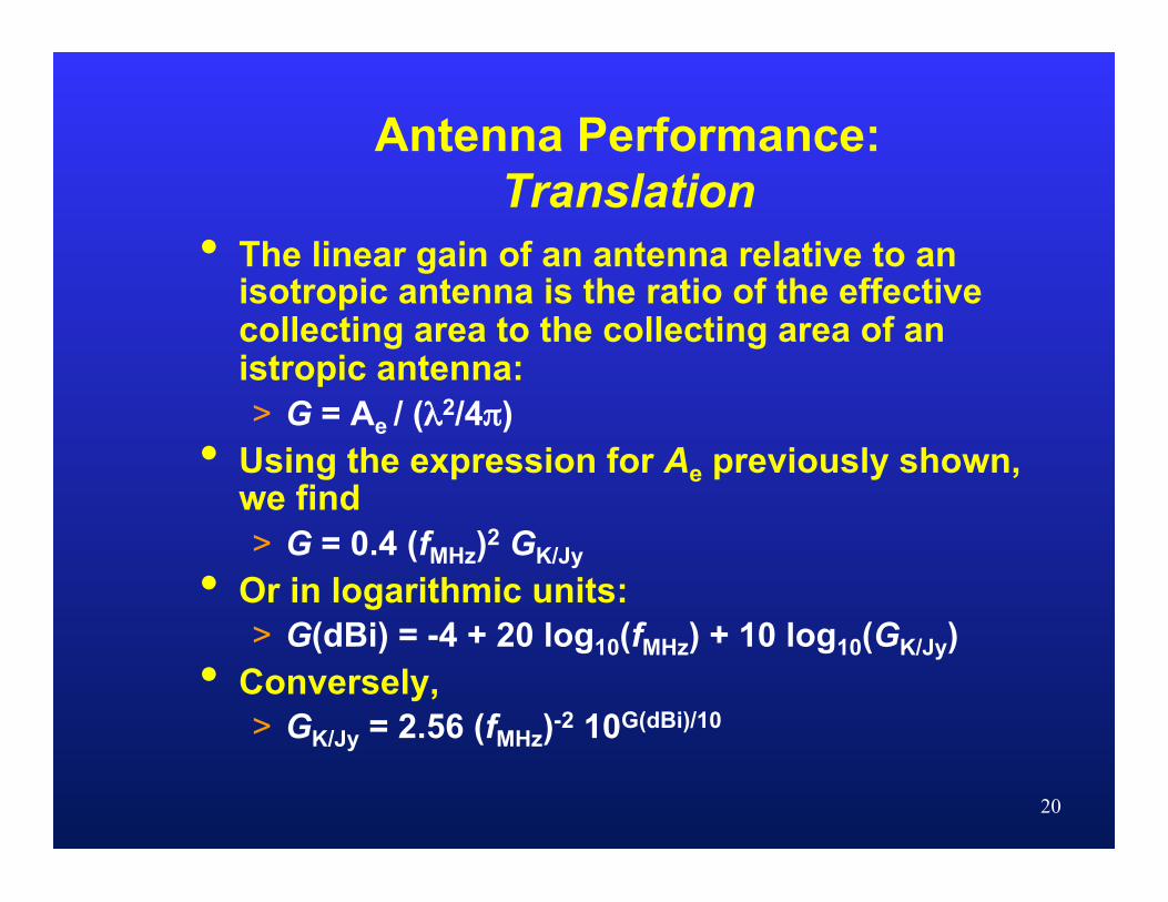
Antenna Performance: Translation

•  The linear gain of an antenna relative to an isotropic antenna is the ratio of the effective collecting area to the collecting area of an istropic antenna: >  G = Ae / (λ2/4π)

•  Using the expression for Ae previously shown, we find >  G = 0.4 (fMHz)2 GK/Jy

•  Or in logarithmic units: >  G(dBi) = -4 + 20 log10(fMHz) + 10 log10(GK/Jy)

•  Conversely, >  GK/Jy = 2.56 (fMHz)-2 10G(dBi)/10

21

Antenna Performance: In Context

•  Cellular Base Antenna @ 1800 MHz >  G = 2.5 x 10-5 K/Jy >  Ae = 0.07 m2

>  G = 15 dBi •  Nobeyama @ 24 GHz

>  G = 0.36 K/Jy >  Ae = 994 m2

>  G = 79 dBi •  Arecibo @ 1400 MHz

>  G = 11 K/Jy >  Ae = 30,360 m2

>  G = 69 dBi

22

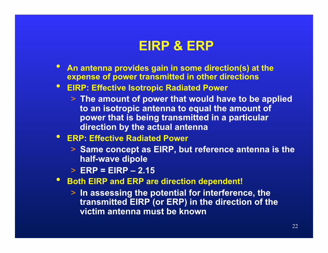
EIRP & ERP •  An antenna provides gain in some direction(s) at the

expense of power transmitted in other directions •  EIRP: Effective Isotropic Radiated Power

>  The amount of power that would have to be applied to an isotropic antenna to equal the amount of power that is being transmitted in a particular direction by the actual antenna

•  ERP: Effective Radiated Power >  Same concept as EIRP, but reference antenna is the

half-wave dipole >  ERP = EIRP – 2.15

•  Both EIRP and ERP are direction dependent! >  In assessing the potential for interference, the

transmitted EIRP (or ERP) in the direction of the victim antenna must be known

Antenna Pattern Example

23

Radio Propagation Basics

Radio propagation

• Propagation is how a signal gets from the transmitting antenna to the receiving antenna

• In the majority of cases, propagation will cause signals to lose strength with… > Distance > Number of obstacles in the path > Frequency > Other factors

Free space loss (FSL)

Surface area of sphere

increases as it expands

Free space loss (FSL)

An antenna of fixed size will intercept a larger fraction of the signal power if it’s closer to the transmitter

Propagation: Free space loss

•  Assumes direct line-of-sight path between transmitter and receiver >  Also assumes no significant blockage of an

imaginary ellipsoidal volume surrounding the direct path, called the first Fresnel zone

Free space loss

First Fresnel zone

Direct ray

Reflected ray

Reflected – Direct = ¼λ

Propagation: Free space loss

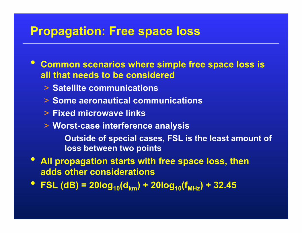
•  Common scenarios where simple free space loss is all that needs to be considered >  Satellite communications >  Some aeronautical communications >  Fixed microwave links >  Worst-case interference analysis

  Outside of special cases, FSL is the least amount of loss between two points

•  All propagation starts with free space loss, then adds other considerations

•  FSL (dB) = 20log10(dkm) + 20log10(fMHz) + 32.45

Propagation: Diffraction

•  Radio waves can bend (diffract) around obstacles •  Amount of diffraction depends on:

>  Frequency   Diffraction is greater at lower frequencies

>  Relative geometry of path and obstacle

  Bigger obstacles require greater bending

>  Composition of obstacle   Diffraction effects depend on

conductivity of obstacle

Propagation: Refraction & Reflection

Refraction

Reflection

Propagation: Scattering

Scattering

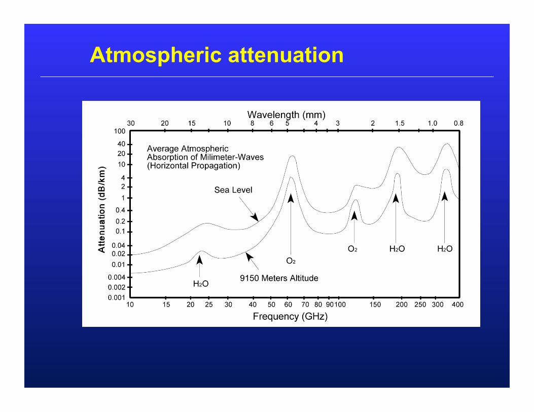
Atmospheric attenuation

Rain attenuation

Interference

Types of interference

•  Co-channel interference >  When the undesired signal fully or partially overlaps

the same channel as the desired signal •  Adjacent-channel or adjacent band interference

>  When the undesired signal is operating on an adjacent or nearby channel or band from the desired signal, but either

  some of the transmitted signal spills over into the desired channel

  the receiver has an undesired response to signals that aren’t on its intended channel

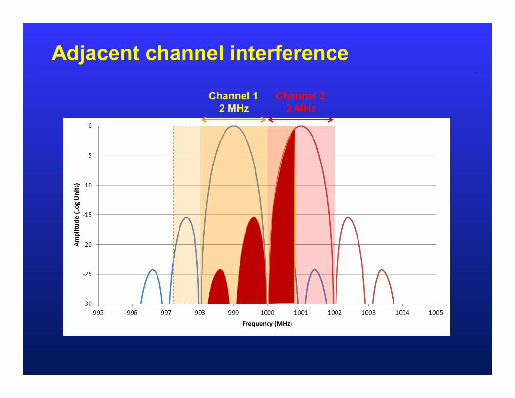
Adjacent channel interference

Channel 1 2 MHz

Channel 2 2 MHz

Transmitter Considerations

Modulation & out-of-band emissions

•  Modulation is the act of imparting information (voice, data, etc.) onto a radio signal

•  When you modulate a signal, it spreads out in frequency

•  This spreading of the signal due to modulation is one reason that transmitted signals impact channels other than their own

Modulation example (BPSK)

Sine wave

+ 1 Mbps digital data (10110...)

= BPSK modulated signal

Signal in Time Signal in Frequency

Spectrum before modulation Spectrum after modulation

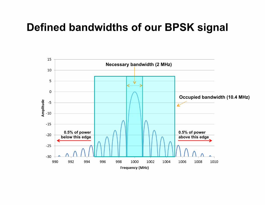
Defined bandwidths of our BPSK signal

Necessary bandwidth (2 MHz)

Occupied bandwidth (10.4 MHz)

0.5% of power above this edge

0.5% of power below this edge

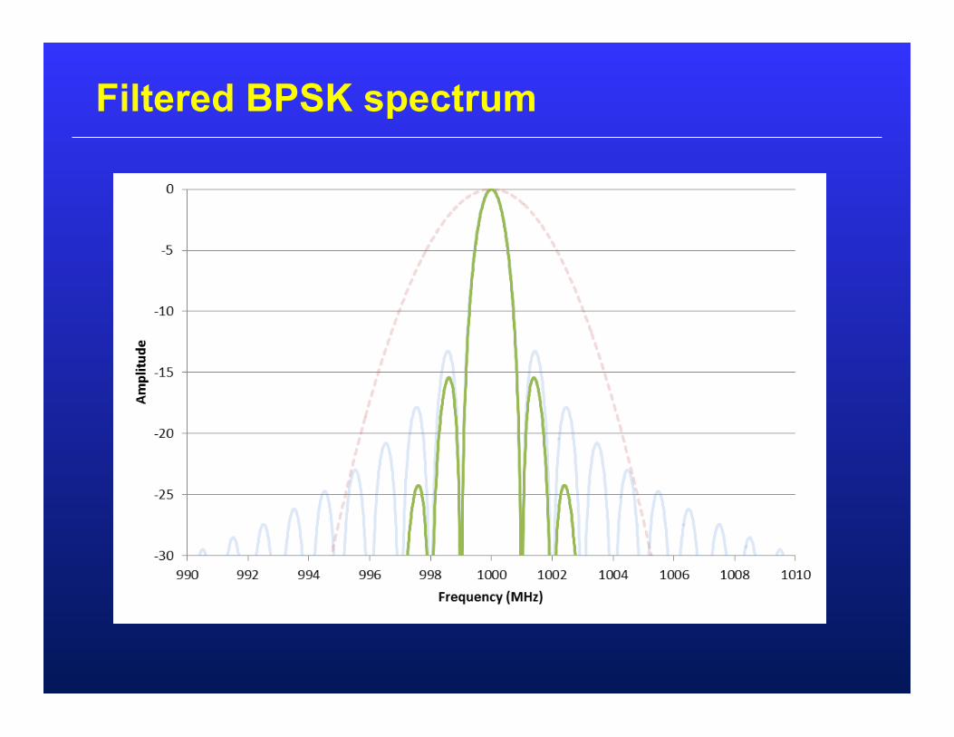
Filtered BPSK spectrum

Filter

Occupied bandwidth after filtering

Necessary bandwidth (2 MHz)

Occupied bandwidth (3.2 MHz)

0.5% of power above this edge

0.5% of power below this edge

Benefits and drawbacks of filters

•  Benefits >  Limits the occupied bandwidth of transmitted

signals, which helps reduce interference to nearby signals

•  Drawbacks >  Distorts signal >  Reduces signal power across desired frequencies >  Requires space, weight, power, and cost to

implement

Bit pattern after filtering

Effect of a 3.3 MHz wide Gaussian filter on a 1 Mbps bit pattern.

Bit pattern before filtering

Bit pattern after applying Gaussian filter

Nonlinearities & spurious emissions

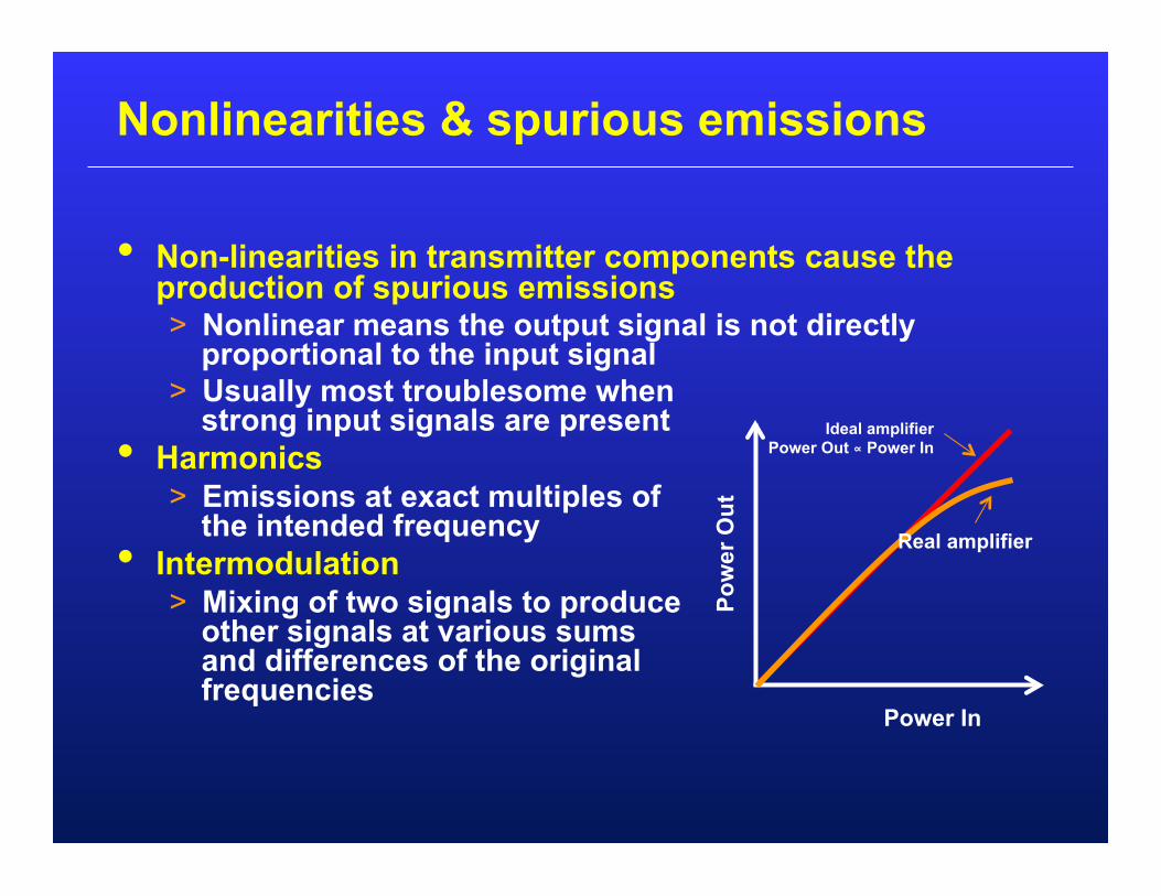
•  Non-linearities in transmitter components cause the production of spurious emissions >  Nonlinear means the output signal is not directly

proportional to the input signal >  Usually most troublesome when

strong input signals are present •  Harmonics

>  Emissions at exact multiples of the intended frequency

•  Intermodulation >  Mixing of two signals to produce

other signals at various sums and differences of the original frequencies

Power In Po

wer

Out

Ideal amplifier Power Out ∝ Power In

Real amplifier

Harmonics and intermodulation

•  Harmonics >  Original signal at frequency f, with

bandwidth df >  2nd harmonic: 2*f, bandwidth 2*df >  3rd harmonic: 3*f, bandwidth 3*df >  Etc.

•  Intermodulation >  Two signals at frequency f1 and f2, each with bandwidth df >  2nd order intermod: f1±f2, bandwidth 2*df >  3rd order intermod: 2f1±f2, 2f2±f1, bandwidth 3*df >  Etc. >  Odd-order intermod products are usually most troublesome

because their frequency can be near f1 and f2

f 2f 3f

Receiver Considerations

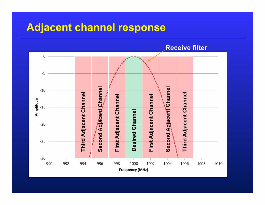
Adjacent channel response

Des

ired

Cha

nnel

Firs

t Adj

acen

t Cha

nnel

Firs

t Adj

acen

t Cha

nnel

Seco

nd A

djac

ent C

hann

el

Seco

nd A

djac

ent C

hann

el

Third

Adj

acen

t Cha

nnel

Third

Adj

acen

t Cha

nnel

Receive filter

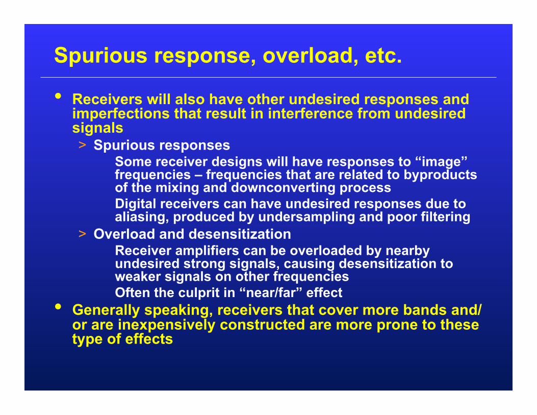
Spurious response, overload, etc.

•  Receivers will also have other undesired responses and imperfections that result in interference from undesired signals >  Spurious responses

  Some receiver designs will have responses to “image” frequencies – frequencies that are related to byproducts of the mixing and downconverting process

  Digital receivers can have undesired responses due to aliasing, produced by undersampling and poor filtering

>  Overload and desensitization   Receiver amplifiers can be overloaded by nearby

undesired strong signals, causing desensitization to weaker signals on other frequencies

  Often the culprit in “near/far” effect •  Generally speaking, receivers that cover more bands and/

or are inexpensively constructed are more prone to these type of effects

Quantifying and Predicting Noise and Interference

Some definitions

•  C: Carrier (desired) signal power, after all filtering by the receiver

•  S: Desired signal power, after all filtering by the receiver. Basically the same as C

•  I: Interference power, after all filtering by the receiver •  N: Receiver system noise power, after all filtering by the

receiver •  N0: Noise power spectral density (noise per bandwidth) •  Eb: For digital systems, the energy per bit, which is the

carrier power divided by the bit rate •  Noise floor: The baseline level of noise in a receiving

system. This is often used to define “N”

Quantifying interference and noise

•  The following ratios (expressed in dB) are often used to quantify the effects of interference and/or noise >  C/I: Ratio of desired Carrier power to Interference power >  C/(I+N): Ratio of desired Carrier power to the total power

caused by Interference and Noise >  C/N: Ratio of desired Carrier power to system Noise >  Eb/N0: For digital systems, the ratio of the Energy per bit

to the power spectral density of Noise >  I/N: Ratio of received Interference power to the Noise

floor of a receiver >  S/N: Normally refers to post-detection ratio of desired

Signal to Noise. For analog voice communications, for example, this would apply to what the user actually hears coming out of the radio’s speaker or headset.

Desired Signal

Undesired Signal

Desired Signal

Overall receiver response

Noise

Desired Signal

Undesired Signal Filter

Desired Signal

Undesired Signal

Noise

Filter

Desired Signal

(Filtered) Undesired Signal (Filtered)

Filtered Noise

Total Interference + Noise

Desired Signal

(Filtered)

What the Receiver Sees

Total Interference + Noise (I+N)

Desired Signal

(C)

C/(I+N) example C/(I+N) ~ 3 dB in this example. Not good.

Predicting performance •  Predicting system performance comes down to estimating C

and I, and measuring N •  Propagation prediction is key to predicting C and I

>  Consistently accurate propagation prediction is virtually impossible except in the simplest of cases

>  Coordination disputes often degenerate into disputes over propagation models

>  For calculating interference, free space loss is often used for worst case analysis, since it is generally the least amount of loss (greatest amount of interference) for a given distance

•  Other coordination considerations include >  the number and distribution of potential interference

sources >  minimum performance metrics (C/I, I/N, etc.) for the victim

receiver >  the fraction of time that the victim system can accept

interference