introduction to satellite remote sensing for air quality

www.nasa.gov

National Aeronautics and

Space Administration

ARSETApplied Remote Sensing Traininghttp://arset.gsfc.nasa.gov

@NASAARSET

Introduction to Satellite Remote

Sensing for Air Quality Applications

Webinar Session 4 – July 27, 2016

NASA Trace Gas Products for Health/Air

Quality Applications

http://arset.gsfc.nasa.gov

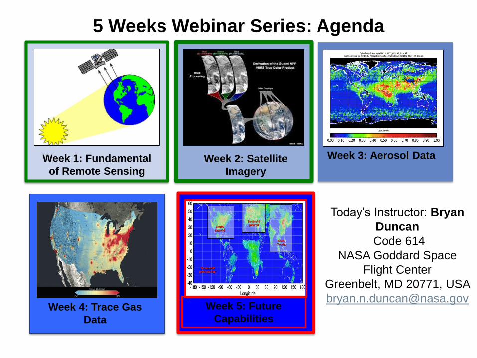
5 Weeks Webinar Series: Agenda

Week 1: Fundamental

of Remote Sensing

Week 2: Satellite

Imagery

Week 3: Aerosol Data

Week 4: Trace Gas

Data

Week 5: Future

Capabilities

Today’s Instructor: Bryan

Duncan

Code 614

NASA Goddard Space

Flight Center

Greenbelt, MD 20771, USA

[email protected]

mailto:[email protected]

www.nasa.gov

National Aeronautics and

Space Administration

ARSETApplied Remote Sensing Traininghttp://arset.gsfc.nasa.gov

@NASAARSET

National Aeronautics and Space Administration

Goddard Space Flight Center Dr. Bryan Duncan

“NASA & Health/Air Quality”

July 27, 2016; ARSET Webinar

http://arset.gsfc.nasa.gov

Some High Level Comments First(with a focus on my research)

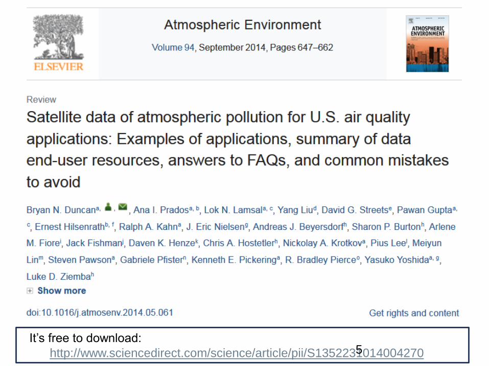
http://www.sciencedirect.com/science/article/pii/S1352231014004270

It’s free to download:5



It’s not free to download:6


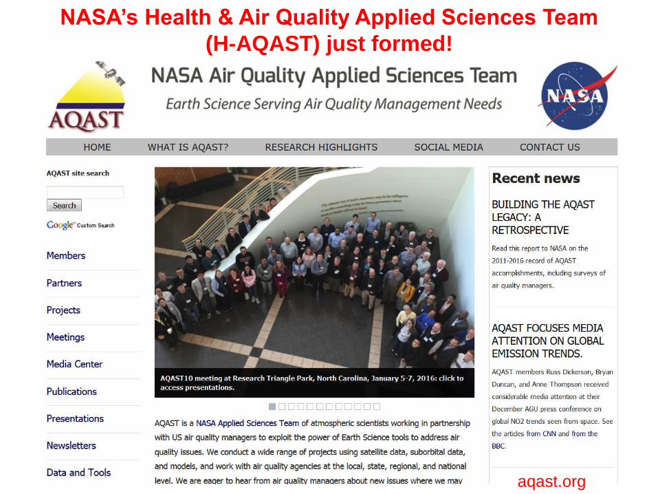
NASA’s Health & Air Quality Applied Sciences Team

(H-AQAST) just formed!

aqast.org

8

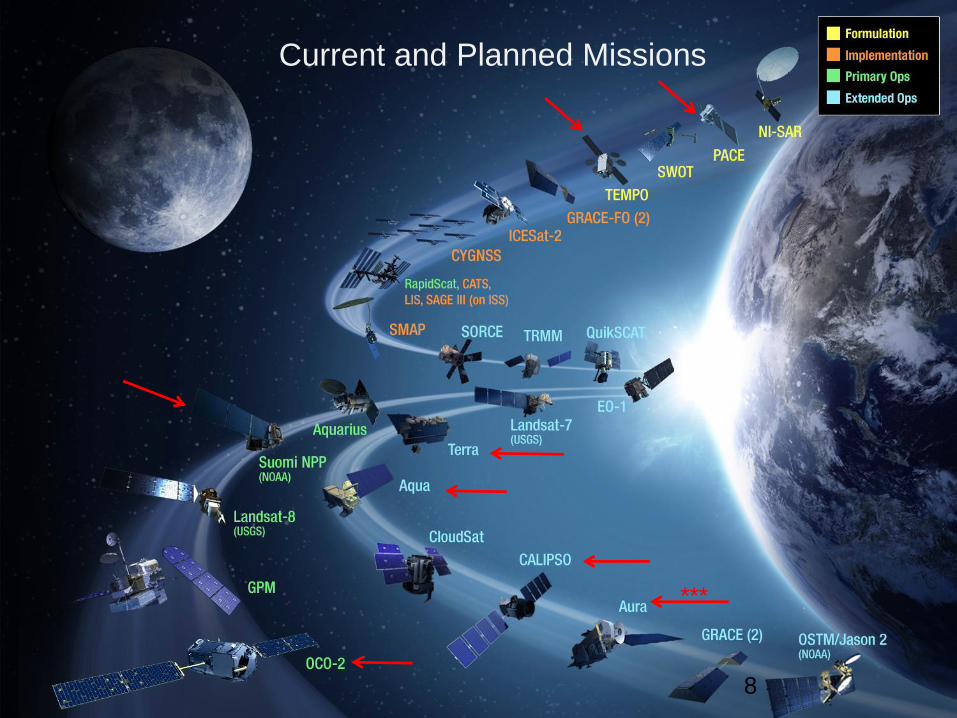
Current and Planned Missions

***

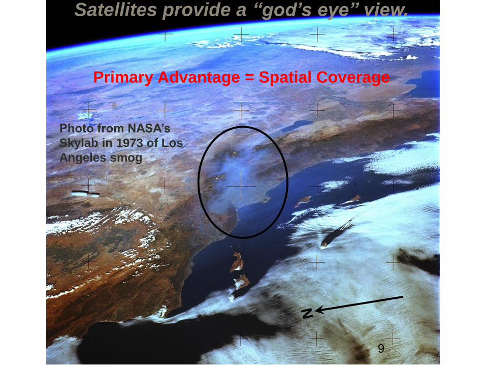
Photo from NASA’s

Skylab in 1973 of Los

Angeles smog

Satellites provide a “god’s eye” view.

Primary Advantage = Spatial Coverage

9

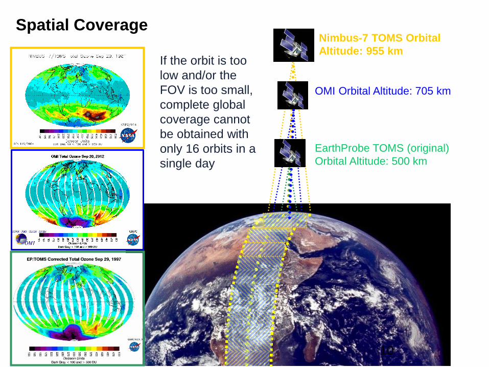
If the orbit is too

low and/or the

FOV is too small,

complete global

coverage cannot

be obtained with

only 16 orbits in a

single day

Nimbus-7 TOMS Orbital

Altitude: 955 km

EarthProbe TOMS (original)

Orbital Altitude: 500 km

OMI Orbital Altitude: 705 km

10

Spatial Coverage

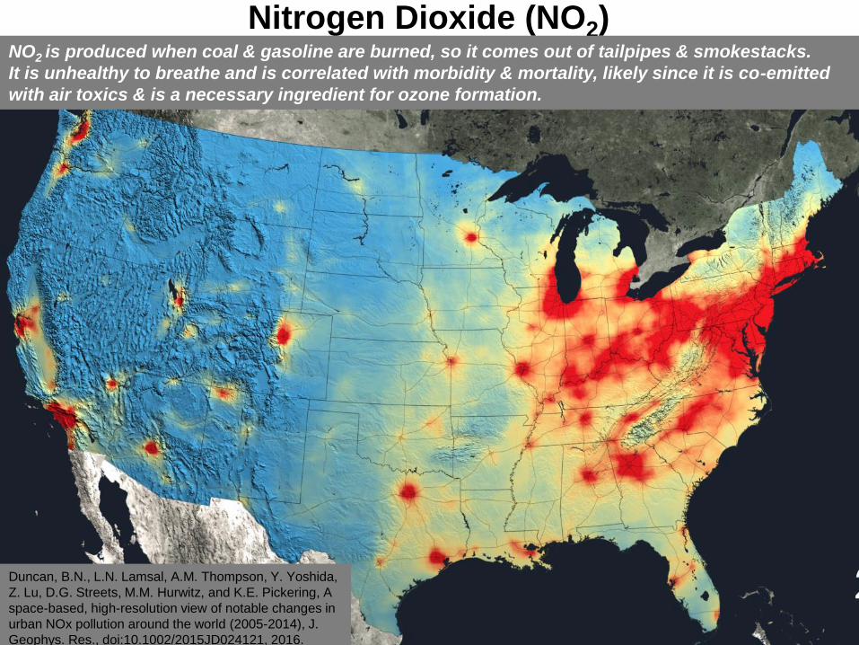
Nitrogen Dioxide (NO2)NO2 is produced when coal & gasoline are burned, so it comes out of tailpipes & smokestacks.

It is unhealthy to breathe and is correlated with morbidity & mortality, likely since it is co-emitted

with air toxics & is a necessary ingredient for ozone formation.

Duncan, B.N., L.N. Lamsal, A.M. Thompson, Y. Yoshida,

Z. Lu, D.G. Streets, M.M. Hurwitz, and K.E. Pickering, A

space-based, high-resolution view of notable changes in

urban NOx pollution around the world (2005-2014), J.

Geophys. Res., doi:10.1002/2015JD024121, 2016.

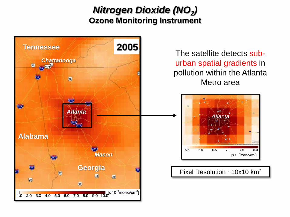
2005

Alabama

Georgia

Tennessee

Atlanta

Macon

Chattanooga

Atlanta

Pixel Resolution ~10x10 km2

Nitrogen Dioxide (NO2)Ozone Monitoring Instrument

The satellite detects sub-

urban spatial gradients in

pollution within the Atlanta

Metro area

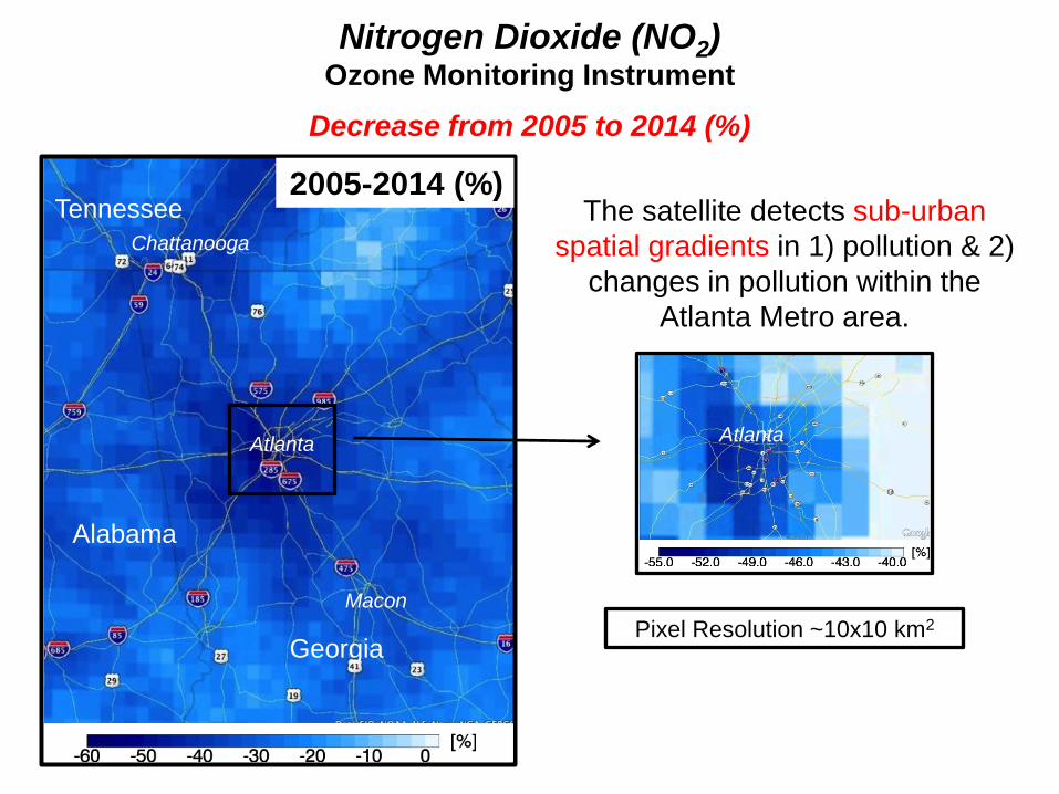
2005-2014 (%)

Decrease from 2005 to 2014 (%)

Georgia

Tennessee

Atlanta Atlanta

Macon

Chattanooga

Macon

Chattanooga

Atlanta

Alabama

Pixel Resolution ~10x10 km2

The satellite detects sub-urban

spatial gradients in 1) pollution & 2)

changes in pollution within the

Atlanta Metro area.

Nitrogen Dioxide (NO2)Ozone Monitoring Instrument

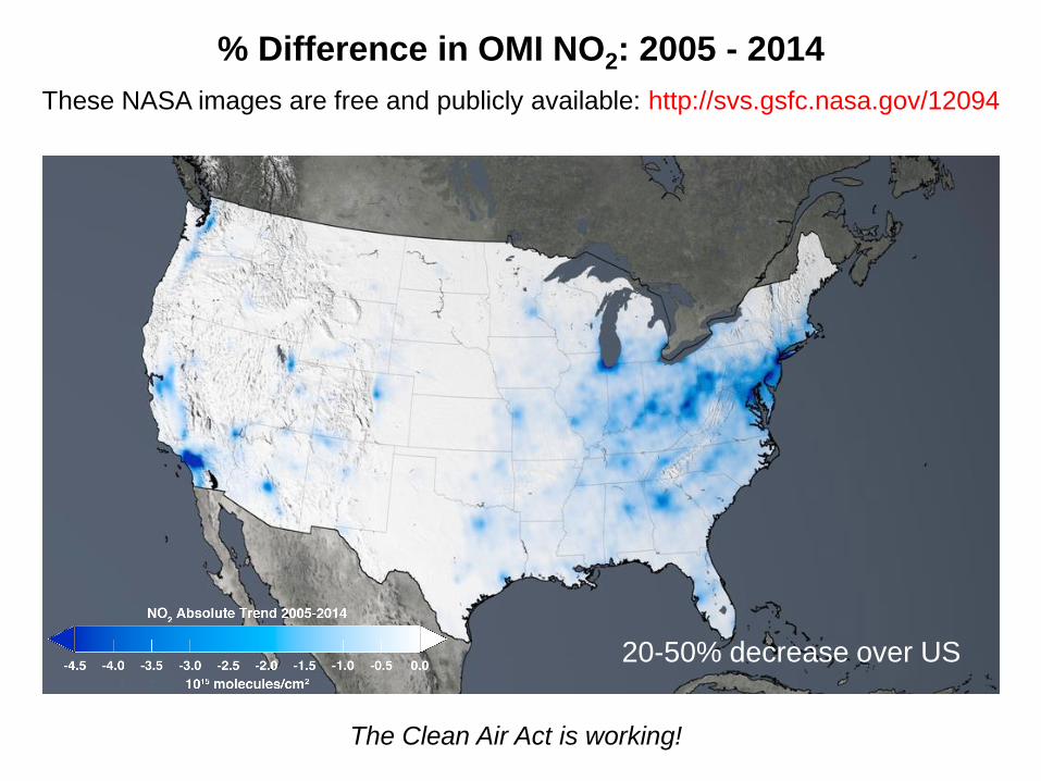
% Difference in OMI NO2: 2005 - 2014

20-50% decrease over US

These NASA images are free and publicly available: http://svs.gsfc.nasa.gov/12094

The Clean Air Act is working!

OMI Detects NO2 Increases from ONG Activities

% Difference OMI NO2

North Dakota

Williston Basin

Suomi NPP VIIRS Lights at Night

Texas

Permian Basin

Eagle Ford

2005-2014

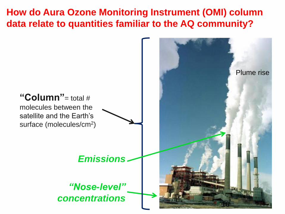
How do Aura Ozone Monitoring Instrument (OMI) column

data relate to quantities familiar to the AQ community?

Emissions

“Nose-level”

concentrations

Plume rise

16

“Column”= total #

molecules between the

satellite and the Earth’s

surface (molecules/cm2)

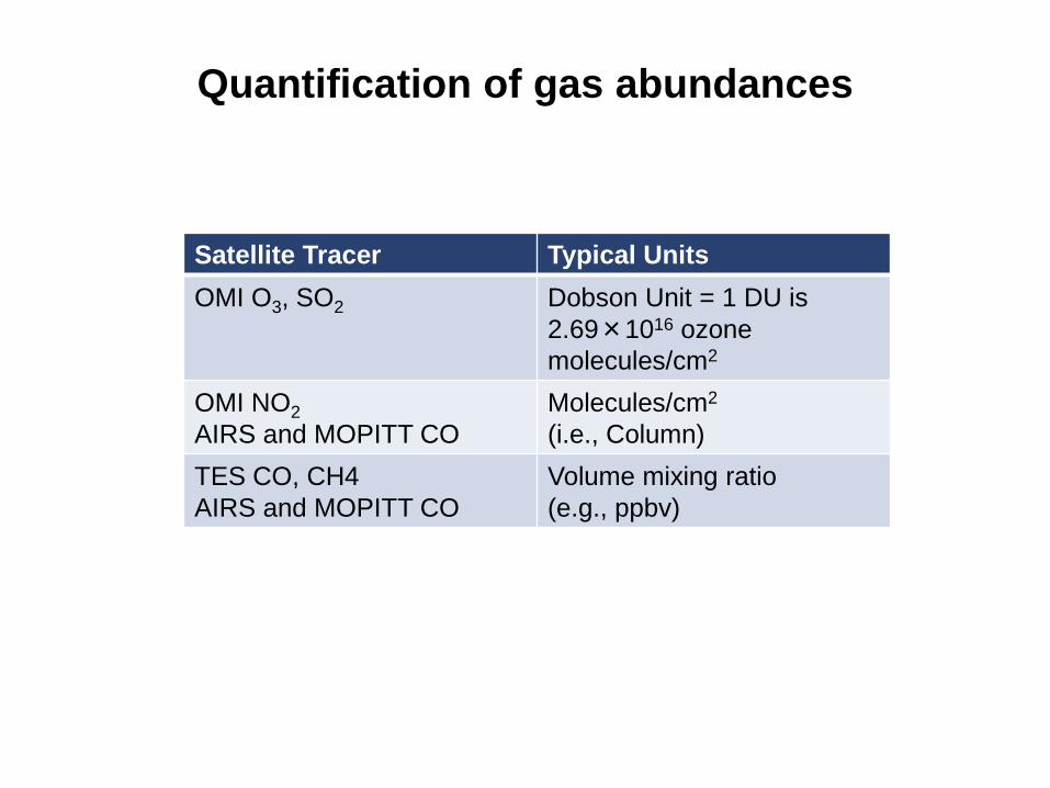
Quantification of gas abundances

Satellite Tracer Typical Units

OMI O3, SO2 Dobson Unit = 1 DU is

2.69×1016 ozone

molecules/cm2

OMI NO2

AIRS and MOPITT CO

Molecules/cm2

(i.e., Column)

TES CO, CH4

AIRS and MOPITT CO

Volume mixing ratio

(e.g., ppbv)

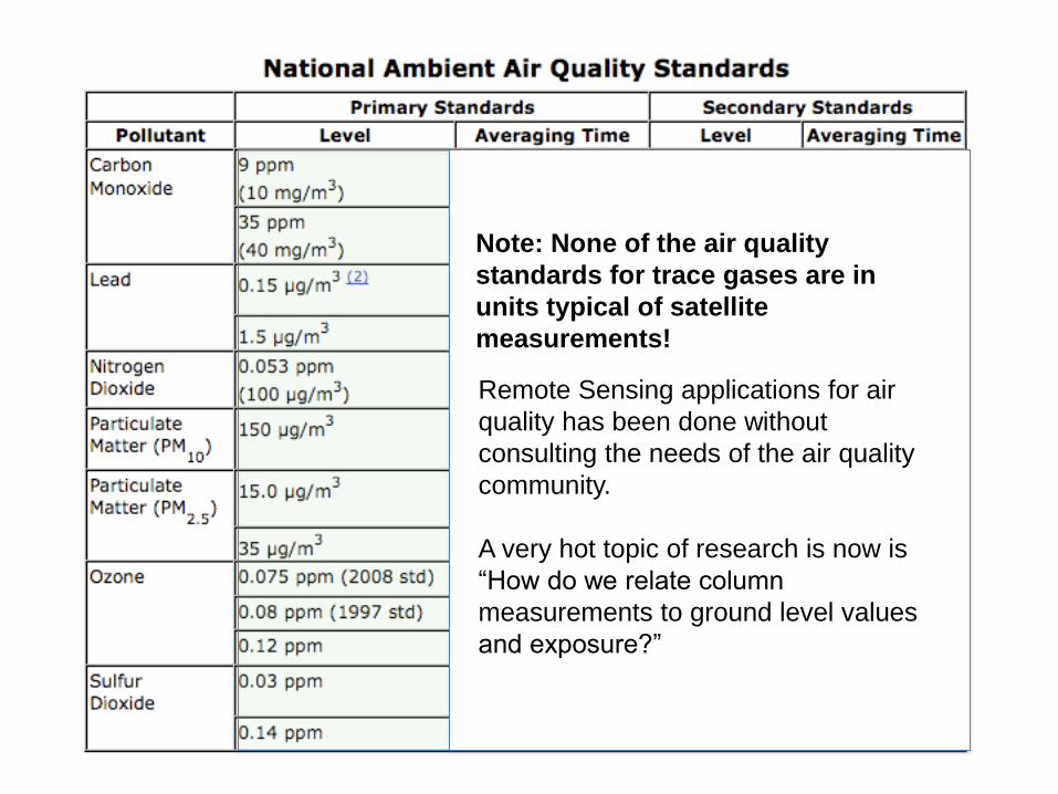
Note: None of the air quality

standards for trace gases are in

units typical of satellite

measurements!

Remote Sensing applications for air

quality has been done without

consulting the needs of the air quality

community.

A very hot topic of research is now is

“How do we relate column

measurements to ground level values

and exposure?”

National Aeronautics and Space Administration 19Applied Remote Sensing Training Program

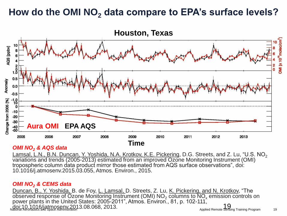
How do the OMI NO2 data compare to EPA’s surface levels?

Houston, Texas

Aura OMI EPA AQS

TimeOMI NO2 & AQS data

Lamsal, L.N., B.N. Duncan, Y. Yoshida, N.A. Krotkov, K.E. Pickering, D.G. Streets, and Z. Lu, “U.S. NO2variations and trends (2005-2013) estimated from an improved Ozone Monitoring Instrument (OMI) tropospheric column data product mirror those estimated from AQS surface observations”, doi: 10.1016/j.atmosenv.2015.03.055, Atmos. Environ., 2015.

OMI NO2 & CEMS data

Duncan, B., Y. Yoshida, B. de Foy, L. Lamsal, D. Streets, Z. Lu, K. Pickering, and N. Krotkov, “The observed response of Ozone Monitoring Instrument (OMI) NO2 columns to NOx emission controls on power plants in the United States: 2005-2011”, Atmos. Environ., 81, p. 102-111, doi:10.1016/jatmosenv.2013.08.068, 2013. 19

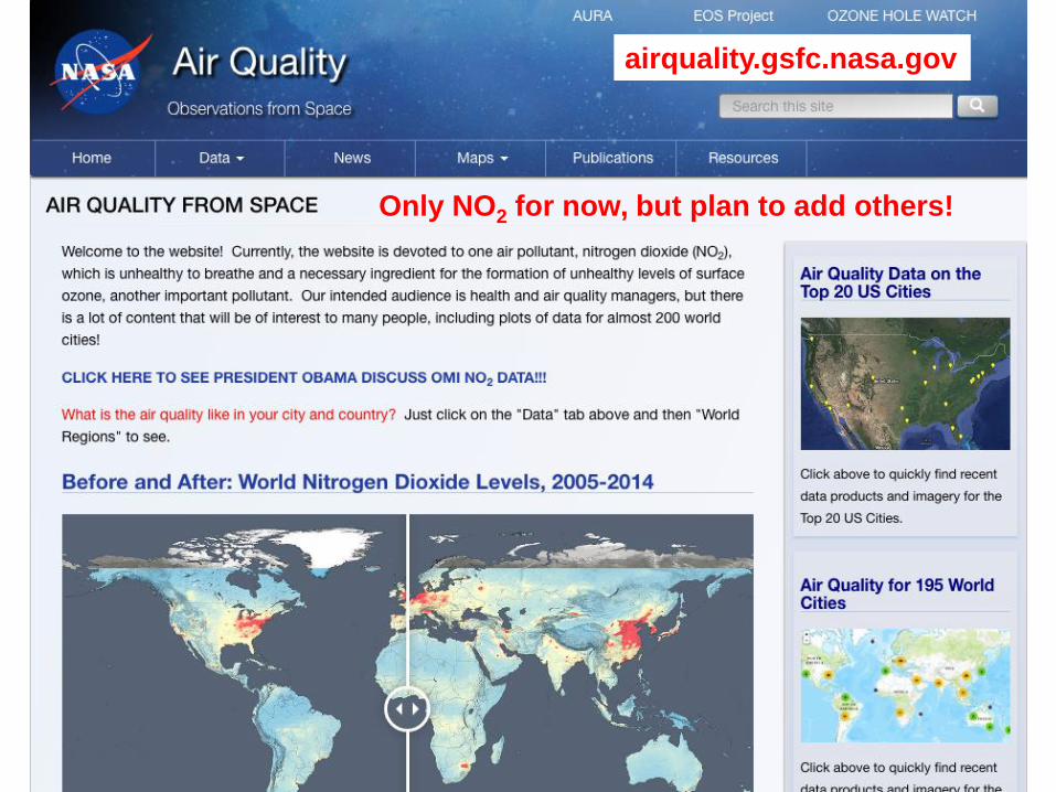
airquality.gsfc.nasa.gov

Only NO2 for now, but plan to add others!

U.S. Trace Gas Data(NO2 isn’t the only game in town!)

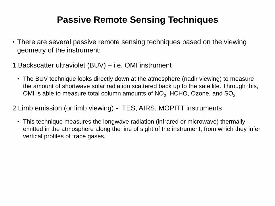
Passive Remote Sensing Techniques

• There are several passive remote sensing techniques based on the viewing

geometry of the instrument:

1.Backscatter ultraviolet (BUV) – i.e. OMI instrument

• The BUV technique looks directly down at the atmosphere (nadir viewing) to measure

the amount of shortwave solar radiation scattered back up to the satellite. Through this,

OMI is able to measure total column amounts of NO2, HCHO, Ozone, and SO2

2.Limb emission (or limb viewing) - TES, AIRS, MOPITT instruments

• This technique measures the longwave radiation (infrared or microwave) thermally

emitted in the atmosphere along the line of sight of the instrument, from which they infer

vertical profiles of trace gases.

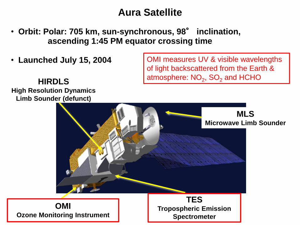
• Orbit: Polar: 705 km, sun-synchronous, 98° inclination, ascending 1:45 PM equator crossing time

• Launched July 15, 2004

Aura Satellite

OMIOzone Monitoring Instrument

TESTropospheric Emission

Spectrometer

HIRDLSHigh Resolution Dynamics

Limb Sounder (defunct)

MLSMicrowave Limb Sounder

OMI measures UV & visible wavelengths

of light backscattered from the Earth &

atmosphere: NO2, SO2 and HCHO

24

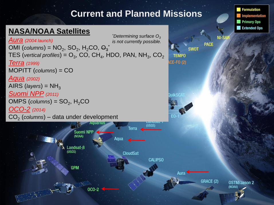
Current and Planned Missions

NASA/NOAA SatellitesAura (2004 launch)

OMI (columns) = NO2, SO2, H2CO, O3*

TES (vertical profiles) = O3, CO, CH4, HDO, PAN, NH3, CO2

Terra (1999)

MOPITT (columns) = CO

Aqua (2002)

AIRS (layers) = NH3

Suomi NPP (2011)

OMPS (columns) = SO2, H2CO

OCO-2 (2014)

CO2 (columns) – data under development

*Determining surface O3

is not currently possible.

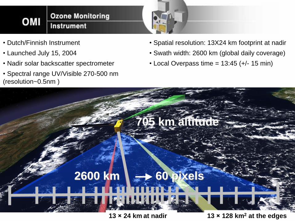
705 km altitude

2600 km 60 pixels

• Dutch/Finnish Instrument

• Launched July 15, 2004

• Nadir solar backscatter spectrometer

• Spectral range UV/Visible 270-500 nm

(resolution~0.5nm )

• Spatial resolution: 13X24 km footprint at nadir

• Swath width: 2600 km (global daily coverage)

• Local Overpass time = 13:45 (+/- 15 min)

13 × 24 km at nadir 13 × 128 km2 at the edges

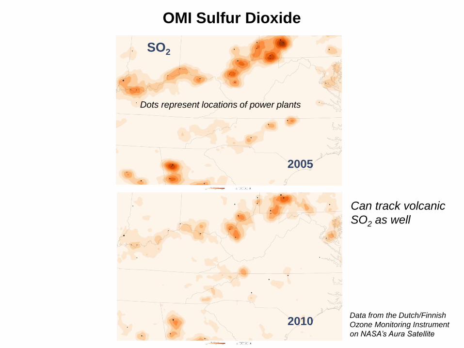
SO2

2010

2005

OMI Sulfur Dioxide

Can track volcanic

SO2 as well

Dots represent locations of power plants

Data from the Dutch/Finnish

Ozone Monitoring Instrument

on NASA’s Aura Satellite

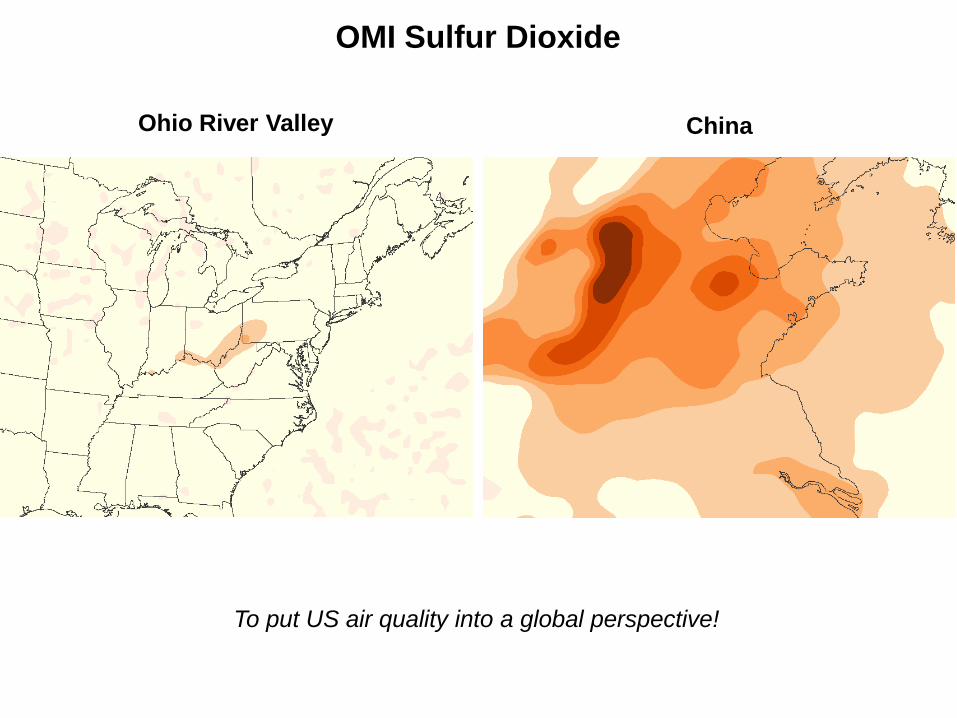
ChinaOhio River Valley

Data from NASA’s Aura Satellite

To put US air quality into a global perspective!

OMI Sulfur Dioxide


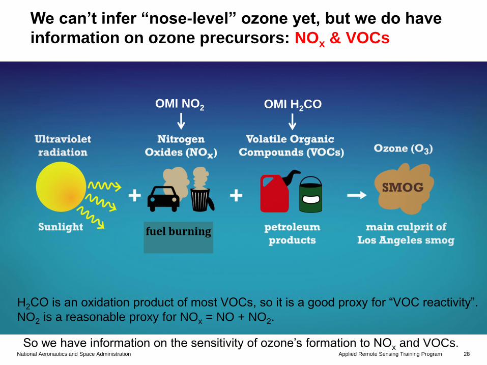
We can’t infer “nose-level” ozone yet, but we do have

information on ozone precursors: NOx & VOCs

fuel burning

OMI NO2 OMI H2CO

So we have information on the sensitivity of ozone’s formation to NOx and VOCs.

H2CO is an oxidation product of most VOCs, so it is a good proxy for “VOC reactivity”.

NO2 is a reasonable proxy for NOx = NO + NO2.

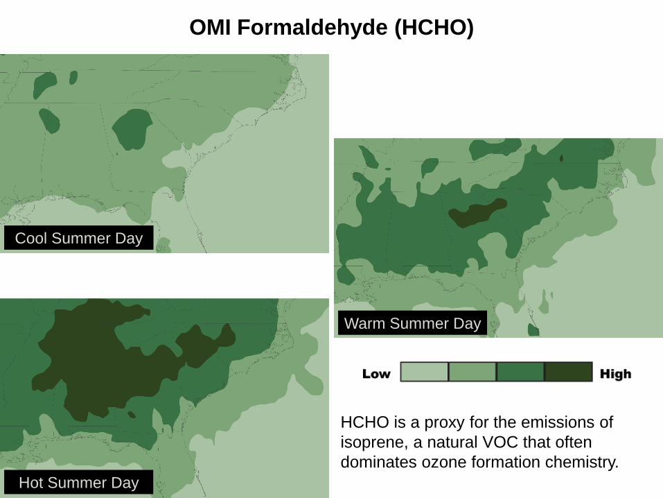
Hot Summer Day

Cool Summer Day

OMI Formaldehyde (HCHO)

Warm Summer Day

HCHO is a proxy for the emissions of

isoprene, a natural VOC that often

dominates ozone formation chemistry.


fuel burning

Reducing VOCs from Cars/Factories is Ineffective

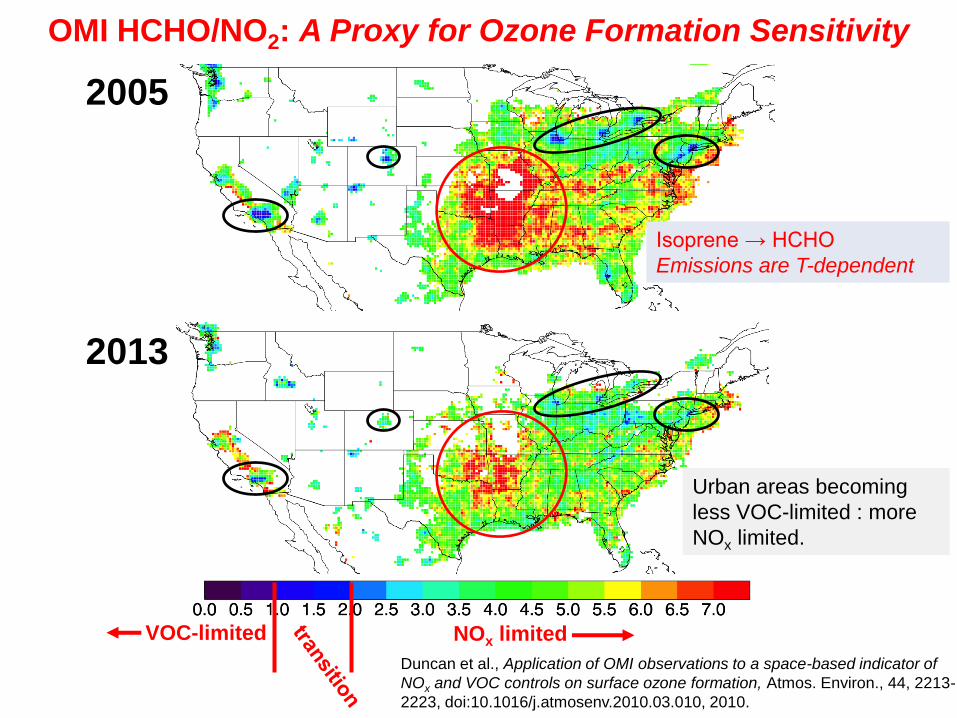
OMI HCHO/NO2: A Proxy for Ozone Formation Sensitivity

VOC-limited NOx limited

Isoprene → HCHO

Emissions are T-dependent

Urban areas becoming

less VOC-limited : more

NOx limited.

2005

2013

Duncan et al., Application of OMI observations to a space-based indicator of

NOx and VOC controls on surface ozone formation, Atmos. Environ., 44, 2213-

2223, doi:10.1016/j.atmosenv.2010.03.010, 2010.

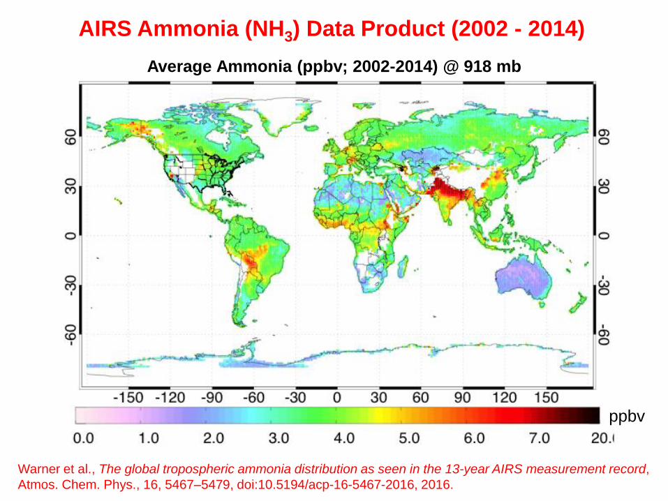
AIRS Ammonia (NH3) Data Product (2002 - 2014)

Average Ammonia (ppbv; 2002-2014) @ 918 mb

ppbv

Warner et al., The global tropospheric ammonia distribution as seen in the 13-year AIRS measurement record,

Atmos. Chem. Phys., 16, 5467–5479, doi:10.5194/acp-16-5467-2016, 2016.

National Aeronautics and Space Administration 33Applied Remote Sensing Training Program33

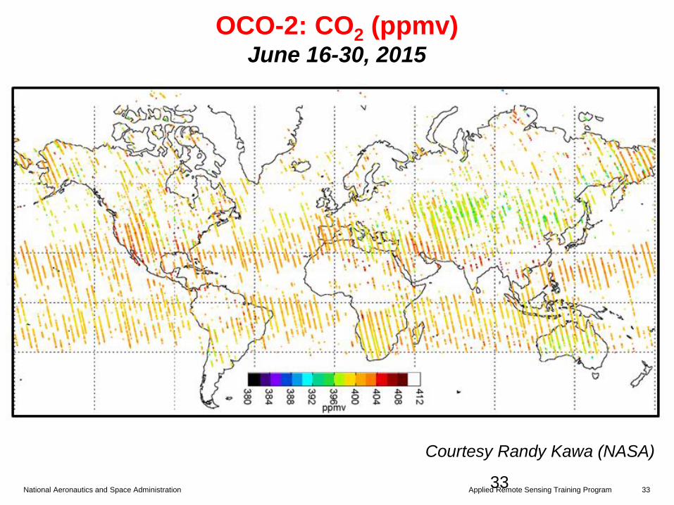
OCO-2: CO2 (ppmv)June 16-30, 2015

Courtesy Randy Kawa (NASA)

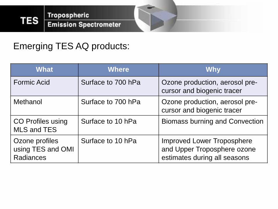
Emerging TES AQ products:

What Where Why

Formic Acid Surface to 700 hPa Ozone production, aerosol pre-

cursor and biogenic tracer

Methanol Surface to 700 hPa Ozone production, aerosol pre-

cursor and biogenic tracer

CO Profiles using

MLS and TES

Surface to 10 hPa Biomass burning and Convection

Ozone profiles

using TES and OMI

Radiances

Surface to 10 hPa Improved Lower Troposphere

and Upper Troposphere ozone

estimates during all seasons


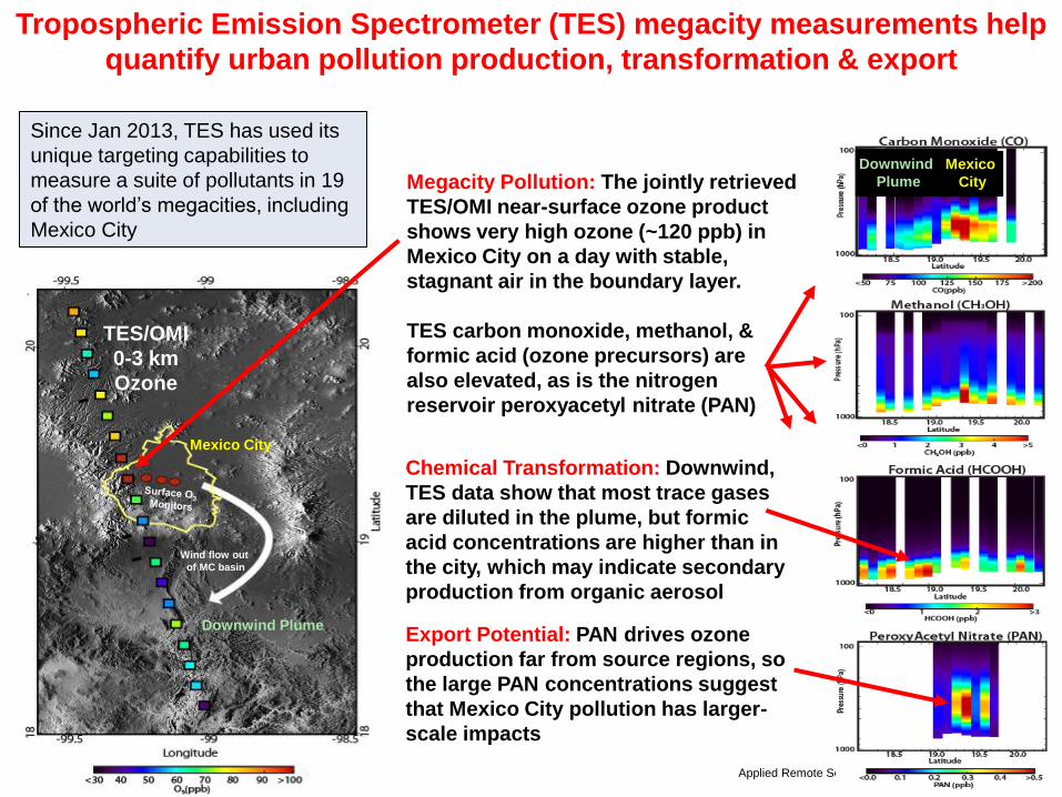
Tropospheric Emission Spectrometer (TES) megacity measurements help

quantify urban pollution production, transformation & export

Since Jan 2013, TES has used its

unique targeting capabilities to

measure a suite of pollutants in 19

of the world’s megacities, including

Mexico City

Surface O3

Monitors

Wind flow out

of MC basin

Chemical Transformation: Downwind,

TES data show that most trace gases

are diluted in the plume, but formic

acid concentrations are higher than in

the city, which may indicate secondary

production from organic aerosol

Export Potential: PAN drives ozone

production far from source regions, so

the large PAN concentrations suggest

that Mexico City pollution has larger-

scale impacts

Megacity Pollution: The jointly retrieved

TES/OMI near-surface ozone product

shows very high ozone (~120 ppb) in

Mexico City on a day with stable,

stagnant air in the boundary layer.

TES carbon monoxide, methanol, &

formic acid (ozone precursors) are

also elevated, as is the nitrogen

reservoir peroxyacetyl nitrate (PAN)

Wind flow out

of MC basin

Mexico City

Downwind Plume

TES/OMI

0-3 km

Ozone

Mexico

City

Downwind

Plume


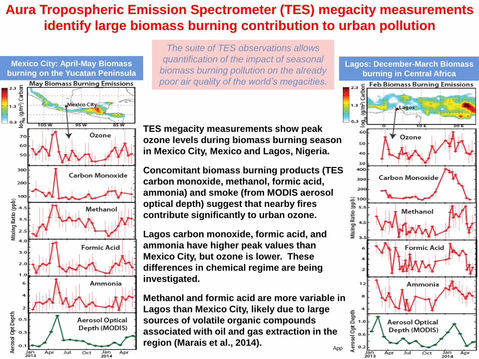
Aura Tropospheric Emission Spectrometer (TES) megacity measurements

identify large biomass burning contribution to urban pollution

Mexico City: April-May Biomass

burning on the Yucatan PeninsulaLagos: December-March Biomass

burning in Central Africa

The suite of TES observations allows

quantification of the impact of seasonal

biomass burning pollution on the already

poor air quality of the world’s megacities.

TES megacity measurements show peak

ozone levels during biomass burning season

in Mexico City, Mexico and Lagos, Nigeria.

Concomitant biomass burning products (TES

carbon monoxide, methanol, formic acid,

ammonia) and smoke (from MODIS aerosol

optical depth) suggest that nearby fires

contribute significantly to urban ozone.

Lagos carbon monoxide, formic acid, and

ammonia have higher peak values than

Mexico City, but ozone is lower. These

differences in chemical regime are being

investigated.

Methanol and formic acid are more variable in

Lagos than Mexico City, likely due to large

sources of volatile organic compounds

associated with oil and gas extraction in the

region (Marais et al., 2014).

“Foreign” Trace Gas Data(ESA, JAXA, etc.!)

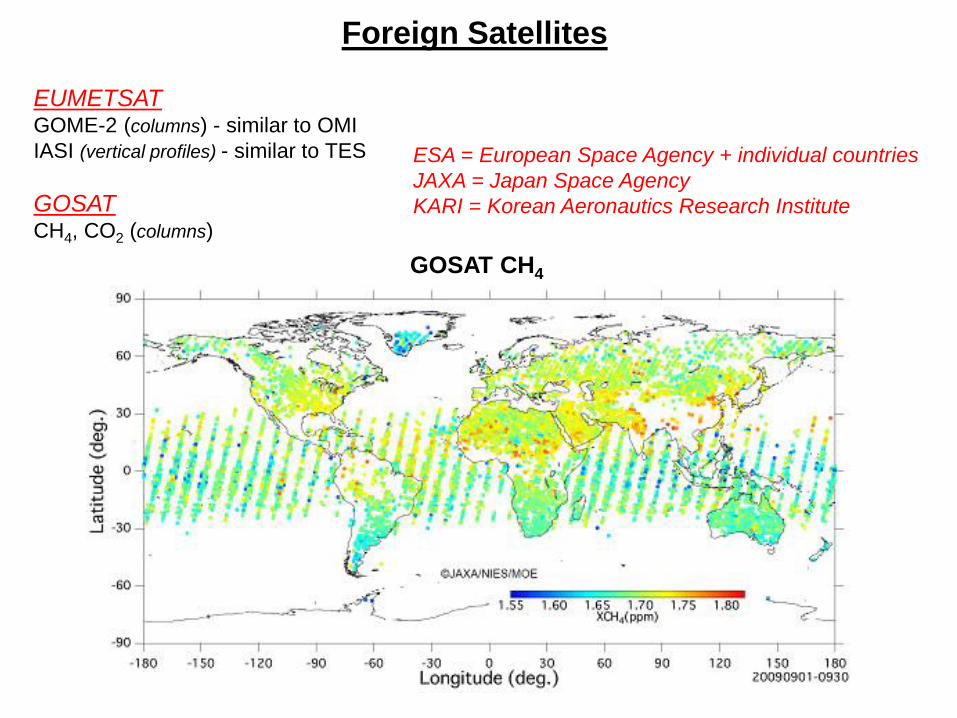
Foreign Satellites

EUMETSATGOME-2 (columns) - similar to OMI

IASI (vertical profiles) - similar to TES

GOSAT CH4, CO2 (columns)

ESA = European Space Agency + individual countries

JAXA = Japan Space Agency

KARI = Korean Aeronautics Research Institute

GOSAT CH4

Future Trace Gas Data(In the works!)


Measuring on Sub-Urban Level

European Space Agency TROPOMIUpcoming

Instruments

TROPOMI Highlights

• Launch 2016

• Observes whole globe

• Sub-urban spatial resolution (7 km x 7 km)

• 1x/day: NO2, ozone (0-2 km vertical),

aerosol, clouds, formaldehyde, glyoxal, SO2,

CO, methane

7x7 km2

13x24 km2

40

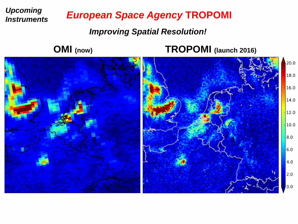
TROPOMI (launch 2016)OMI (now)

Improving Spatial Resolution!

European Space Agency TROPOMIUpcoming

Instruments

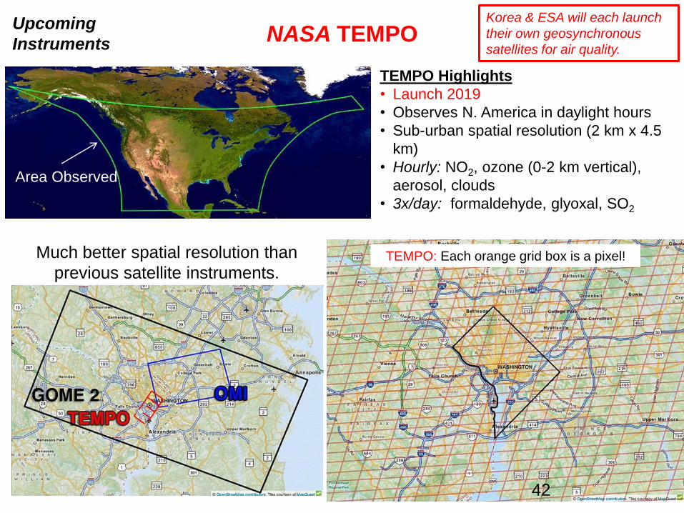
TEMPO: Each orange grid box is a pixel!

TEMPO Highlights

• Launch 2019

• Observes N. America in daylight hours

• Sub-urban spatial resolution (2 km x 4.5

km)

• Hourly: NO2, ozone (0-2 km vertical),

aerosol, clouds

• 3x/day: formaldehyde, glyoxal, SO2

Area Observed

Much better spatial resolution than

previous satellite instruments.

42

Korea & ESA will each launch

their own geosynchronous

satellites for air quality.NASA TEMPO

Upcoming

Instruments

Some Fundamentals(Things to know about satellite data!)


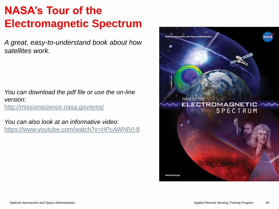
NASA’s Tour of the

Electromagnetic Spectrum

A great, easy-to-understand book about how

satellites work.

You can download the pdf file or use the on-line

version:

http://missionscience.nasa.gov/ems/

You can also look at an informative video:

https://www.youtube.com/watch?v=HPcAWNlVl-8

http://missionscience.nasa.gov/ems/

https://www.youtube.com/watch?v=HPcAWNlVl-8

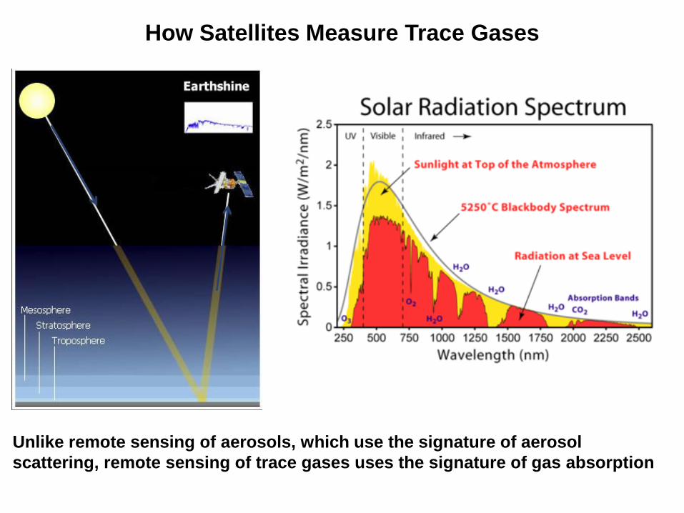
Unlike remote sensing of aerosols, which use the signature of aerosol

scattering, remote sensing of trace gases uses the signature of gas absorption

How Satellites Measure Trace Gases

Satellite Measurements Take Advantage of Distinct

Absorption Spectra

1

Ozone

2

316-340nm

1

NO2

2

405-465nm

1

SO2

2

305-330nm

UV-A VisibleUV-BUV-C

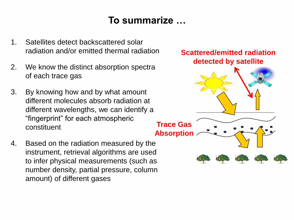
To summarize …

1. Satellites detect backscattered solar

radiation and/or emitted thermal radiation

2. We know the distinct absorption spectra

of each trace gas

3. By knowing how and by what amount

different molecules absorb radiation at

different wavelengths, we can identify a

“fingerprint” for each atmospheric

constituent

4. Based on the radiation measured by the

instrument, retrieval algorithms are used

to infer physical measurements (such as

number density, partial pressure, column

amount) of different gases

Trace Gas

Absorption

Scattered/emitted radiation

detected by satellite

http://www-as.harvard.edu/chemistry/trop/satellite/index.html


48

Trace Gas

Concentration

and

Absorption

May vary

Throughout

The column

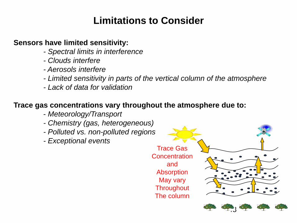
Sensors have limited sensitivity:

- Spectral limits in interference

- Clouds interfere

- Aerosols interfere

- Limited sensitivity in parts of the vertical column of the atmosphere

- Lack of data for validation

Trace gas concentrations vary throughout the atmosphere due to:

- Meteorology/Transport

- Chemistry (gas, heterogeneous)

- Polluted vs. non-polluted regions

- Exceptional events

Limitations to Consider



• Column and/or layer product

• Where in the column there is sensitivity

• If it is a layer product, what the vertical resolution of the layers is

• How the products average horizontally, vertically and temporally

• Product and pixel resolution

• Product coverage

• Measurement frequency

• Overpass time

Proper Use of Remote Sensing Products Requires

Knowledge of:

Satellite data are powerful for health and air quality applications.

However, it is very important to understand the strengths and limitations of the data

for a particular application.

Without proper knowledge, it is very easy to misuse and abuse the data!

Please do not be afraid to ask for help, information, guidance, etc.

There are many resources available to the data end-user. Make use of them!!!

Final Remarks

NO ASSIGNMENTS


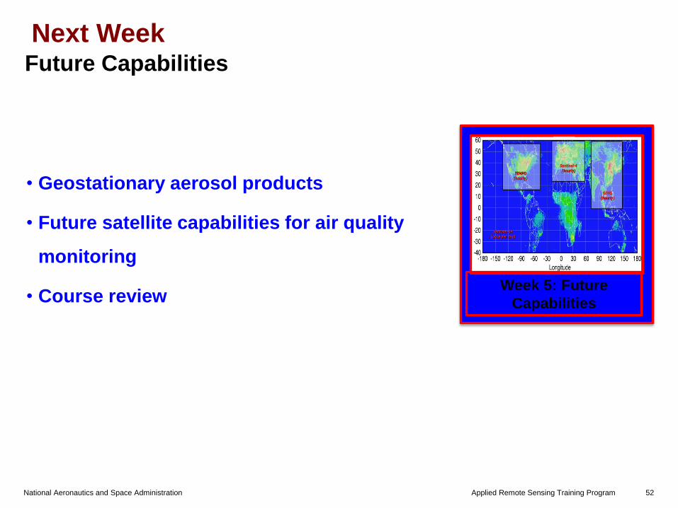
Next Week

• Geostationary aerosol products

• Future satellite capabilities for air quality

monitoring

• Course review

Future Capabilities

Week 5: Future

Capabilities

All the materials and recordings

will be available at

http://arset.gsfc.nasa.gov/airquality/webin

ars/introduction-satellite-remote-sensing-

air-quality-applications

Contact Pawan Gupta ([email protected]) for the technical questions

Brock Blevins ([email protected]) for material access, future trainings, and other logistic

http://arset.gsfc.nasa.gov/airquality/webinars/introduction-satellite-remote-sensing-air-quality-applications



introduction to satellite remote sensing for air quality

Documents