introduction to scienti c computing · 2014-12-14 · 2 contents preface this script has been...
TRANSCRIPT

Introduction to Scientific Computing
A Compact Course
Walter Gander, ETH Zurich
December 15 -19, 2014Brno University

2

Contents
Chapter 1. Finite Precision Arithmetic. Matlab, Octave, Maple 31.1 Real Numbers and Machine Numbers . . . . . . . . . . . . . . 41.2 The IEEE Standard . . . . . . . . . . . . . . . . . . . . . . . 51.3 Rounding Errors . . . . . . . . . . . . . . . . . . . . . . . . . 8
1.3.1 Standard Model of Arithmetic . . . . . . . . . . . . . 81.3.2 Cancellation . . . . . . . . . . . . . . . . . . . . . . . 9
1.4 Condition of a Problem . . . . . . . . . . . . . . . . . . . . . 111.5 Stable and Unstable Algorithms . . . . . . . . . . . . . . . . . 13
1.5.1 Forward Stability . . . . . . . . . . . . . . . . . . . . . 131.5.2 Backward Stability . . . . . . . . . . . . . . . . . . . . 15
1.6 Machine Independent Algorithms . . . . . . . . . . . . . . . . 161.6.1 Computing the square-root . . . . . . . . . . . . . . . 161.6.2 Computing the Exponential Function . . . . . . . . . 17
1.7 Problems . . . . . . . . . . . . . . . . . . . . . . . . . . . . . 20
Chapter 2. Linear Systems of Equations (direct and iterativesolver) . . . . . . . . . . . . . . . . . . . . . . . . . . . . . . . . . . . 23
2.1 Gaussian Elimination . . . . . . . . . . . . . . . . . . . . . . . 232.2 Elimination with Givens-Rotations . . . . . . . . . . . . . . . 282.3 Iterative Solver for Large Sparse Systems . . . . . . . . . . . 31
2.3.1 Fixed Point Form . . . . . . . . . . . . . . . . . . . . . 322.3.2 Residual, Error and the Difference of Iterates . . . . . 322.3.3 Convergence Criteria . . . . . . . . . . . . . . . . . . . 342.3.4 Convergence Factor and Convergence Rate . . . . . . 35
2.4 Classical Stationary Iterative Methods . . . . . . . . . . . . . 362.4.1 Jacobi . . . . . . . . . . . . . . . . . . . . . . . . . . . 372.4.2 Gauss-Seidel . . . . . . . . . . . . . . . . . . . . . . . 372.4.3 Successive Over-relaxation (SOR) . . . . . . . . . . . 382.4.4 Richardson . . . . . . . . . . . . . . . . . . . . . . . . 42
2.5 Nonstationary Iterative Methods . . . . . . . . . . . . . . . . 432.5.1 Conjugate Residuals . . . . . . . . . . . . . . . . . . . 432.5.2 Steepest Descent . . . . . . . . . . . . . . . . . . . . . 442.5.3 The Conjugate Gradient Method . . . . . . . . . . . . 45

4 CONTENTS
2.5.4 Arnoldi Process . . . . . . . . . . . . . . . . . . . . . . 512.5.5 Solving Linear Equations with Arnoldi . . . . . . . . . 55
2.6 Problems . . . . . . . . . . . . . . . . . . . . . . . . . . . . . 57
Chapter 3. Nonlinear Equations . . . . . . . . . . . . . . . . . . . 613.1 Bisection . . . . . . . . . . . . . . . . . . . . . . . . . . . . . 613.2 Fixed Point Iteration . . . . . . . . . . . . . . . . . . . . . . . 623.3 Convergence Rates . . . . . . . . . . . . . . . . . . . . . . . . 653.4 Zeros of Polynomials . . . . . . . . . . . . . . . . . . . . . . . 73
3.4.1 Condition of the Zeros . . . . . . . . . . . . . . . . . . 743.4.2 Companion Matrix . . . . . . . . . . . . . . . . . . . . 773.4.3 Newton Method for Real Simple Zeros . . . . . . . . . 783.4.4 Fractal . . . . . . . . . . . . . . . . . . . . . . . . . . . 83
3.5 Nonlinear Systems of Equations . . . . . . . . . . . . . . . . . 843.5.1 Fixed Point Iteration . . . . . . . . . . . . . . . . . . . 863.5.2 Newton’s Method . . . . . . . . . . . . . . . . . . . . . 863.5.3 Continuation Methods . . . . . . . . . . . . . . . . . . 92
3.6 Problems . . . . . . . . . . . . . . . . . . . . . . . . . . . . . 92
Chapter 4. Least Squares . . . . . . . . . . . . . . . . . . . . . . . 954.1 Linear Least Squares Problem and the Normal Equations . . 974.2 Singular Value Decomposition (SVD) . . . . . . . . . . . . . . 100
4.2.1 Pseudoinverse . . . . . . . . . . . . . . . . . . . . . . . 1034.2.2 Fundamental Subspaces . . . . . . . . . . . . . . . . . 1044.2.3 Solution of the Linear Least Squares Problem . . . . . 1064.2.4 SVD and Rank . . . . . . . . . . . . . . . . . . . . . . 107
4.3 Condition of the Linear Least Squares Problem . . . . . . . . 1094.4 Algorithms Using Orthogonal Matrices . . . . . . . . . . . . . 112
4.4.1 QR Decomposition . . . . . . . . . . . . . . . . . . . . 1124.4.2 Method of Householder . . . . . . . . . . . . . . . . . 1134.4.3 Method of Givens . . . . . . . . . . . . . . . . . . . . 116
4.5 Nonlinear Least Squares Problems . . . . . . . . . . . . . . . 1174.5.1 Notations and Definitions . . . . . . . . . . . . . . . . 1184.5.2 Newton’s Method . . . . . . . . . . . . . . . . . . . . . 1204.5.3 Gauss-Newton Method . . . . . . . . . . . . . . . . . . 1234.5.4 Levenberg-Marquardt Algorithm . . . . . . . . . . . . 124
4.6 Linear Least Squares Problems with Linear Constraints . . . 1274.6.1 Solution with SVD . . . . . . . . . . . . . . . . . . . . 1294.6.2 Classical Solution Using Lagrange Multipliers . . . . . 1334.6.3 Direct Elimination of the Constraints . . . . . . . . . 134
4.7 Problems . . . . . . . . . . . . . . . . . . . . . . . . . . . . . 137

Contents 5
Chapter 5. Numerical Ordinary Differential Equations . . . . 1395.1 Notation, Existence of Solutions . . . . . . . . . . . . . . . . 1395.2 Analytical and Numerical Solutions . . . . . . . . . . . . . . . 1415.3 Euler’s Method . . . . . . . . . . . . . . . . . . . . . . . . . . 1435.4 Reduction to First Order System . . . . . . . . . . . . . . . . 1465.5 Slope Field, Methods of Euler and Heun . . . . . . . . . . . . 1485.6 Local Truncation Error and Order of a Method . . . . . . . . 1505.7 Construction of One-step Methods of Runge Kutta Type . . . 152
5.7.1 Runge-Kutta Methods for s = 2 . . . . . . . . . . . . 1535.7.2 Order and Global Error . . . . . . . . . . . . . . . . . 1555.7.3 The classical Runge Kutta Method . . . . . . . . . . . 156
5.8 Derivation of Runge Kutta Methods using Maple . . . . . . 1565.9 Embedded Runge-Kutta Methods, Stepsize Control . . . . . . 1595.10 Adaptive Integration . . . . . . . . . . . . . . . . . . . . . . . 1625.11 Problems . . . . . . . . . . . . . . . . . . . . . . . . . . . . . 165

Contents
2 CONTENTS
Preface
This script has been compiled for an intensive winter course, given by theauthor at Masarik University in Brno, December 15 to 19, 2014. The materialfor the five mornings of four hours of lectures is taken from our book, whichrecently appeared in Springer Verlag:
Walter Gander, Martin J. Gander, Felix Kwok: Scien-tific Computing, an Introduction using Maple and Matlab, SpringerVerlag, April 2014, ISBN 978-3-319-04324-1
In the present script we have omitted many proofs which can be found inthe book. Time is too short in this intensive course to discuss them. Wetherefore concentrate on important facts and on algorithms.
Zurich, November 2014, Walter Gander

Chapter 1. Finite Precision Arithmetic.Matlab, Octave, Maple
In this lecture series we shall perform computations with floating point num-bers using the IEEE-standard. Matlab, the language of technical comput-ing is very well suited for such computations. It is a commercial productwhich emerged from the intention of Cleve Moler to simplify the use of theLINPACK and EISPACK libraries for teaching numerical linear algebra atthe University of New Mexico more than 30 years ago. Cleve Moler calledhis interface MATrix LABoratory and used the acronym MATLAB. TodayMatlab is a powerful tool used worldwide in scientific computing. There areclones in public domain, notably GNU Octave and Scilab which can serve wellfor beginners without violating software licenses. However, full compatibilitywith Matlab is not guaranteed.
Numerical computing is affected by rounding errors. For instance thenumber π truncated to an IEEE floating point number is
>> pi
ans =
3.141592653589793
>> sin(pi)
ans =
1.224646799147353e-16
In finite arithmetic we cannot expect to get sinπ = 0 as we know frommathematics. There were already some 50 years ago first developments ofcomputer algebra systems which would do computations not only in extendedprecision but also sybolically. Maple is one of those systems. These systemsknow the constant π as we can see here
sum(1/k^2, k=1..infinity);
1
6π2
sin(Pi);
0
For numerical computations we can ask such a system for an extended numberof digits:
Digits:=50;

4 FINITE PRECISION ARITHMETIC. MATLAB, OCTAVE, MAPLE
50
p:=evalf(Pi);
3.1415926535897932384626433832795028841971693993751
sin(p);
-51
5.8209749445923078164062862089986280348253421170680 10
But also with more digits we cannot avoid rounding errors!
1.1 Real Numbers and Machine Numbers
Every computer is a finite automaton. This implies that a computer can onlystore a finite set of numbers and perform only a finite number of operations.In mathematics, we are used to calculating with real numbers R covering thecontinuous interval (−∞,∞), but on the computer, we must contend with adiscrete, finite set of machine numbers M = −amin, . . . , amax. Hence eachreal number a has to be mapped onto a machine number a to be used ona computer. In fact a whole interval of real numbers is mapped onto onemachine number as shown in Figure 1.1.
Figure 1.1.Mapping of real numbers R onto machine numbers M
Nowadays, machine numbers are often represented in the binary system.In general, any base (or radix ) B could be used to represent numbers. A realmachine number or floating point number consists of two parts, a mantissam and an exponent e
a = ±m×Bem = D.D · · ·D mantissae = D · · ·D exponent
where D ∈ 0, 1, . . . , B− 1 stands for one digit. To make the representationof machine numbers unique (note that e.g. 1.2345× 103 = 0.0012345× 10⁶),we require for a machine number a 6= 0 that the first digit before the decimalpoint in the mantissa be nonzero; such numbers are called normalized. Onedefining characteristic for any finite precision arithmetic is the number ofdigits used for the mantissa and the exponent: the number of digits in theexponent defines the range of the machine numbers, whereas the numbers ofdigits in the mantissa defines the precision.
The precision of the machine is described by the real machine numbereps. Historically, eps is defined to be the smallest positive a ∈ M such that

The IEEE Standard 5
a + 1 6= 1 when the addition is carried out on the computer. Because thisdefinition involves details about the behavior of floating point addition, whichare not easily accessible, a newer definition of eps is simply the spacing ofthe floating point numbers between 1 and B (usually B = 2). The currentdefinition only relies on how the numbers are represented.
In the computer algebra system Maple, numerical computations are per-formed in base 10. The number of digits of the mantissa is defined by thevariable Digits, which can be freely chosen. The number of digits of theexponent is given by the word length of the computer — for 32-bit machines,we have a huge maximal exponent of u = 231 = 2147483648.
1.2 The IEEE Standard
Since 1985 we have for computer hardware the ANSI/IEEE Standard 754for Floating Point Numbers. It has been adopted by almost all computermanufacturers. The base is B = 2. Expressed as decimal numbers thisstandard allows to represent numbers with about 16 decimal digits and anexponent of 3-digits. More precisely the computation range is the interval
M = [−amin, amax] = [−1.797693134862316e+308, 1.797693134862316e+308]
The standard defines single and double precision floating point numbers.Matlab computes by default with double precision. We shall not discussthe single precision which uses 32 bits.
The IEEE double precision floating point standard representation uses a64-bit word with bits numbered from 0 to 63 from left to right. The first bitS is the sign bit, the next eleven bits E are the exponent bits for e and thefinal 52 bits F represent the mantissa m:
S
e︷ ︸︸ ︷EEEEEEEEEEE
m︷ ︸︸ ︷FFFFF · · ·FFFFF
0 1 11 12 63
The value a represented by the 64-bit word is defined as follows:
normal numbers: If 0 < e < 2047, then a = (−1)S × 2e−1023 × 1.m where1.m is the binary number created by prefixing m with an implicit lead-ing 1 and a binary point.
subnormal numbers: If e = 0 and m 6= 0, then a = (−1)S×2−1022×0.m ,which are denormalized numbers.
If e = 0 and m = 0 and S = 1, then a = −0
If e = 0 and m = 0 and S = 0, then a = 0
exceptions: If e = 2047 and m 6= 0, then a = NaN (Not a number) )
If e = 2047 and m = 0 and S = 1, then a = −InfIf e = 2047 and m = 0 and S = 0, then a = Inf

6 FINITE PRECISION ARITHMETIC. MATLAB, OCTAVE, MAPLE
By using the hexadecimal format in Matlab we can see the internalrepresentation. For example
>> format hex
>> 2
ans = 4000000000000000
If we expand each hexadecimal digit to 4 binary digits we obtain for thenumber 2:
0100 0000 0000 0000 0000 0000 .... 0000 0000 0000
We skipped with .... seven groups of four zero binary digits. The interpre-tation is: +1× 21024−1023 × 1.0 = 2.
>> 6.5
ans = 401a000000000000
This means
0100 0000 0001 1010 0000 0000 .... 0000 0000 0000
Again we skipped with .... seven groups of four zeros. The resulting numberis +1× 21025−1023 × (1 + 1
2 + 18 ) = 6.5.
From now on, our discussion will stick to the IEEE Standard as usedin Matlab. In other, more low-level programming languages, the behaviorof the IEEE arithmetic can be adapted, e.g. the exception handling can beexplicitly specified.
• The machine precision is eps = 2−52.
• The largest machine number amax is denoted by realmax. Note that
>> realmax
ans = 1.7977e+308
>> log2(ans)
ans = 1024
>> 2^1024
ans = Inf
This looks like a contradiction at first glance, since the largest exponentshould be 22046−1023 = 21023 according the IEEE conventions. Butrealmax is the number with the largest possible exponent and with themantissa F consisting of all ones:
>> format hex
>> realmax
ans = 7fefffffffffffff

The IEEE Standard 7
This is
V = +1× 22046−1023 × 1. 11 . . . 1︸ ︷︷ ︸52Bits
= 21023 ×
(1 +
(1
2
)1
+
(1
2
)2
+ · · ·+(
1
2
)52)
= 21023 ×1−
(12
)531−
(12
) = 21023 × (2− eps)
Even though Matlab reports log2(realmax)=1024, realmax does notequal 21024, but rather (2−eps)×21023; taking the logarithm of realmaxyields 1024 only because of rounding. Similar rounding effects wouldalso occur for machine numbers that are a bit smaller than realmax.
• The computation range is the interval [−realmax, realmax]. If an op-eration produces a result outside this interval, then it is said to overflow.Before the IEEE Standard, computation would halt with an error mes-sage in such a case. Now the result of an overflow operation is assignedthe number ±Inf.
• The smallest positive normalized number is realmin = 2−1022.
• IEEE allows computations with denormalized numbers. The positivedenormalized numbers are in the interval [realmin ∗ eps, realmin]. Ifan operation produces a strictly positive number that is smaller thanrealmin ∗ eps, then this result is said to be in the underflow range.Since such a result cannot be represented, zero is assigned instead.
• When computing with denormalized numbers, we may suffer a loss ofprecision. Consider the following Matlab program:
>> format long
>> res=pi*realmin/123456789101112
res = 5.681754927174335e-322
>> res2=res*123456789101112/realmin
res2 = 3.15248510554597
>> pi = 3.14159265358979
The first result res is a denormalized number, and thus can no longerbe represented with full accuracy. So when we reverse the operationsand compute res2, we obtain a result which only contains 2 correct dec-imal digits. We therefore recommend avoiding the use of denormalizednumbers whenever possible.

8 FINITE PRECISION ARITHMETIC. MATLAB, OCTAVE, MAPLE
1.3 Rounding Errors
1.3.1 Standard Model of Arithmetic
Let a and b be two machine numbers; then c = a× b will in general not be amachine number anymore, since the product of two numbers contains twiceas many digits. The computed result will therefore be rounded to a machinenumber c which is closest to c.
As an example, consider the 8-digit decimal numbers
a = 1.2345678 and b = 1.1111111,
whose product is
c = 1.37174198628258 and c = 1.3717420.
The absolute rounding error is the difference ra = c− c = 1.371742e−8, and
r =rac
= 1e−8
is called the relative rounding error.On today’s computers, basic arithmetic operations obey the standard
model of arithmetic: for a, b ∈M, we have
a⊕b = (a⊕ b)(1 + r), (1.1)
where r is the relative rounding error with |r| < eps, the machine precision.We denote with ⊕ ∈ +,−,×, / the exact basic operation and with ⊕ theequivalent computer operation.
Another interpretation of the standard model of arithmetic is due toWilkinson. In what follows, we will no longer use the multiplication sym-bol × for the exact operation; it is common practice in algebra to denotemultiplication without any symbol: ab⇐⇒ a× b. Consider the operations
Addition: a+b = (a+ b)(1 + r) = (a+ ar) + (b+ br) = a+ b
Subtraction: a−b = (a− b)(1 + r) = (a+ ar)− (b+ br) = a− b
Multiplication: a×b = ab(1 + r) = a(b+ br) = ab
Division: a/b = (a/b)(1 + r) = (a+ ar)/b = a/b
In each of the above, the operation satisfies
Wilkinson’s Principle
The result of a numerical computation on the computer is theexact result with slightly perturbed initial data.
For example, the numerical result of the multiplication a×b is the exactresult ab with a slightly perturbed operand b = b + br. As a consequenceof Wilkinson’s Principle, we need to study the effect that slightly perturbeddata have on the result of a computation.

Rounding Errors 9
1.3.2 Cancellation
A special rounding error is called cancellation. If we subtract two almostequal numbers, leading digits are canceled. Consider the following two num-bers with 5 decimal digits:
1.2345e0−1.2344e0
0.0001e0 = 1.0000e−4
If the two numbers were exact, the result delivered by the computer wouldalso be exact. But if the first two numbers had been obtained by previouscalculations and were affected by rounding errors, then the result would atbest be 1.XXXXe−4, where the digits denoted by X are unknown.
Example: we want to write a Matlab function which computes the realsolutions of a quadratic equation
x2 + px+ q = 0.
If the solutions turn out to be complex then an error message should bewritten.
A naive approach is to use the textbook formula
x1,2 = −p2±√(p
2
)2− q.
We obtain the function
function [x1,x2]=QuadEquationNaive(p,q)
discriminant=(p/2)^2-q;
if discriminant<0
error(’solutions are complex’)
end
d=sqrt(discriminant);
x1=-p/2+d; x2=-p/2-d;
We check this program for some test examples:
• (x− 2)(x+ 3) = x2 + x− 6 = 0
>> [x1,x2]=QuadEquationNaive(1,-6)
x1=2, x2=-3 correct
• (x− 109)(x+ 2 · 10−9) = x2 + (2 · 10−9 − 109)x+ 2
>> [x1,x2]=QuadEquationNaive(2e-9-1e9,2)
x1=1.0000e+09, x2=0 wrong

10 FINITE PRECISION ARITHMETIC. MATLAB, OCTAVE, MAPLE
• (x+ 10200)(x− 1) = x2 + (10200 − 1)x− 10200
>> [x1,x2]=QuadEquationNaive(1e200-1,-1e200)
x1=Inf, x2=-Inf wrong
Why do we get wrong answers? When looking at the textbook formulawe notice that for large |p| forming p2 may overflow. This is the case in thethird example.
On the other hand for small q the formula is
x1,2 = −p2±√(p
2
)2− q ≈ −p
2± p
2
and one solution is affected by cancellation. This is the case in the secondexample.
We can avoid the overflow by factoring out. The cancellation can beavoided by computing first the solution which has the larger absolute valueand then use the relation of Vieta:
x1x2 = q
to compute the smaller solution without cancellation. Thus instead of thetextbook formula we use
x1 = −sign(p)
(|p|/2 + |p|
√1
4− q/p/p
)x2 = q/x1 Vieta
We obtain the function
function [x1,x2]=QuadraticEq(p,q)
if abs(p/2)>1 % avoid overflow
factor=abs(p); discriminant=0.25-q/p/p; % by factoring out
else
factor=1; discriminant=(p/2)^2-q;
end
if discriminant<0
error(’Solutions are complex’)
else
x1=abs(p/2)+factor*sqrt(discriminant); % compute larger solution
if p>0, x1=-x1; end % adapt sign
if x1== 0, x(2)=0;
else
x2=q/x1; % avoid cancellation
end % for smaller solution
end

Condition of a Problem 11
This time we get
• (x− 2)(x+ 3) = x2 + x− 6 = 0
>> [x1,x2]=QuadraticEq(1,-6)
x1 = 2, x2 = -3 correct
• (x− 109)(x+ 2 · 10−9) = x2 + (2 · 10−9 − 109)x+ 2
>> [x1,x2]=QuadraticEq(2e-9-1e9,2)
x1=1.0000e+09, x2=2.0000e-09 correct!
• (x+ 10200)(x− 1) = x2 + (10200 − 1)x− 10200
>> [x1,x2]=QuadraticEq(1e200-1,-1e200)
x1=-1.0000e+200, x2=1 correct!
1.4 Condition of a Problem
Intuitively, the conditioning of a problem measures how sensitive it is tosmall changes in the data; if the problem is very sensitive, it is inherentlymore difficult to solve it using finite precision arithmetic.
Definition 1.1. (Condition Number) The condition number κ of aproblem P : Rn → Rm is the smallest number such that
|xi − xi||xi|
≤ ε for 1 ≤ i ≤ n =⇒ ‖P(x)− P(x)‖‖P(x)‖
≤ κε+ o(ε), (1.2)
where o(ε) represents terms that are asymptotically smaller than ε.
A problem is well conditioned if κ is not too large; otherwise the problemis ill conditioned. Well-conditioned means that the solution of the problemwith slightly perturbed data does not differ much from the solution of theproblem with the original data. Ill-conditioned problems are problems forwhich the solution is very sensitive to small changes in the data.
Example 1.1. We consider the problem of multiplying two real numbers,P(x1, x2) := x1x2. If we perturb the data slightly, say
x1 := x1(1 + ε1), x2 := x2(1 + ε2), |εi| ≤ ε, i = 1, 2,
we obtain
x1x2 − x1x2x1x2
= (1 + ε1)(1 + ε2)− 1 = ε1 + ε2 + ε1ε2,
12 FINITE PRECISION ARITHMETIC. MATLAB, OCTAVE, MAPLE
and since we assumed that the perturbations are small, ε 1, we can neglectthe product ε1ε2 compared to the sum ε1 + ε2, and we obtain
|x1x2 − x1x2||x1x2|
≤ 2ε.
Hence the condition number of multiplication is κ = 2, and the problem ofmultiplying two real numbers is well conditioned.
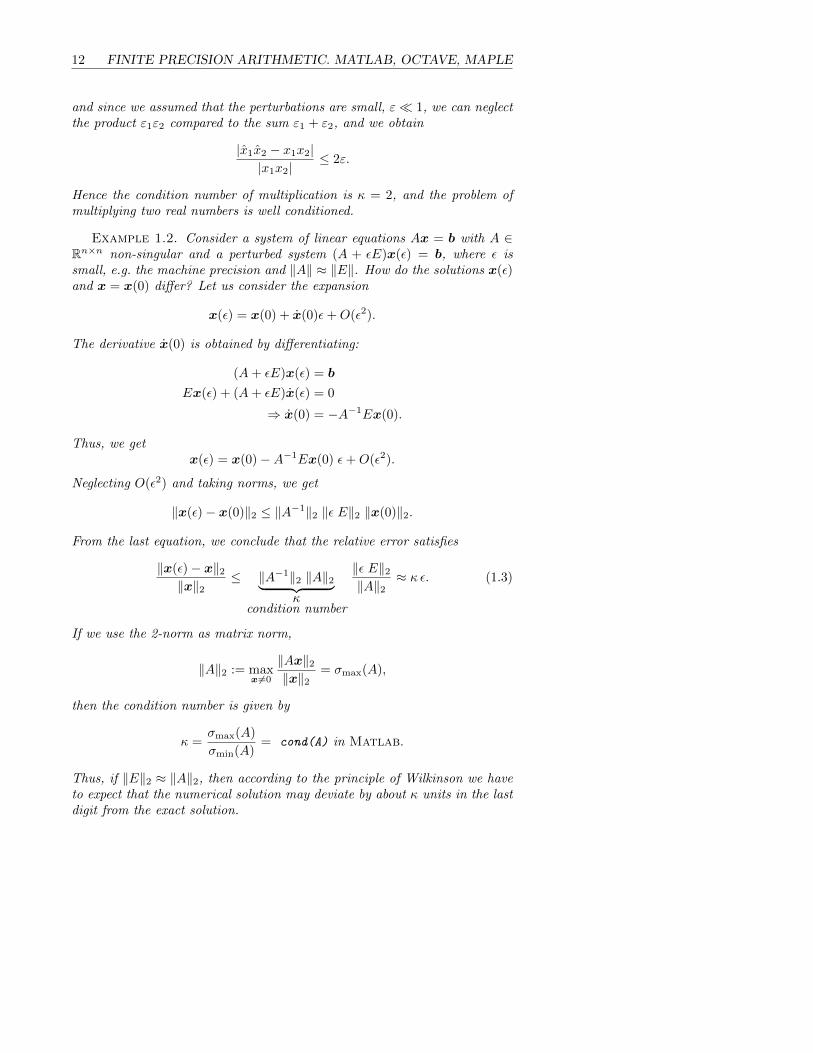
Example 1.2. Consider a system of linear equations Ax = b with A ∈Rn×n non-singular and a perturbed system (A + εE)x(ε) = b, where ε issmall, e.g. the machine precision and ‖A‖ ≈ ‖E‖. How do the solutions x(ε)and x = x(0) differ? Let us consider the expansion
x(ε) = x(0) + x(0)ε+O(ε2).
The derivative x(0) is obtained by differentiating:
(A+ εE)x(ε) = b
Ex(ε) + (A+ εE)x(ε) = 0
⇒ x(0) = −A−1Ex(0).
Thus, we getx(ε) = x(0)−A−1Ex(0) ε+O(ε2).
Neglecting O(ε2) and taking norms, we get
‖x(ε)− x(0)‖2 ≤ ‖A−1‖2 ‖ε E‖2 ‖x(0)‖2.
From the last equation, we conclude that the relative error satisfies
‖x(ε)− x‖2‖x‖2
≤ ‖A−1‖2 ‖A‖2︸ ︷︷ ︸κ
condition number
‖ε E‖2‖A‖2
≈ κ ε. (1.3)
If we use the 2-norm as matrix norm,
‖A‖2 := maxx6=0
‖Ax‖2‖x‖2
= σmax(A),
then the condition number is given by
κ =σmax(A)
σmin(A)= cond(A) in Matlab.
Thus, if ‖E‖2 ≈ ‖A‖2, then according to the principle of Wilkinson we haveto expect that the numerical solution may deviate by about κ units in the lastdigit from the exact solution.

Stable and Unstable Algorithms 13
Numerical experiment:
>> A=[21.6257 51.2930 1.5724 93.4650
5.2284 83.4314 37.6507 84.7163
68.3400 3.6422 6.4801 52.5777
67.7589 4.5447 42.3687 9.2995];
>> x=[1:4]’; b=A*x;
>> xa=A\b;
>> format long
>> [xa x]
ans =
0.999999999974085 1.000000000000000
1.999999999951056 2.000000000000000
3.000000000039628 3.000000000000000
4.000000000032189 4.000000000000000
>> cond(A)
ans =
6.014285987494785e+05
>> eps*cond(A)
ans =
1.335439755999431e-10
The condition number of A is 6.014e5 so we must expect that 5 decimal digitswill be affected by numerical errors. This is indeed the case as we can see,the relative error is about εκ(A).
1.5 Stable and Unstable Algorithms
An algorithm for solving a given problem P : Rn −→ R is a sequence ofelementary operations,
P(x) = fn(fn−1(. . . f2(f1(x)) . . .)).
In general, there exist several different algorithms for a given problem.
1.5.1 Forward Stability
If the amplification of the error in the operation fi is given by the corre-sponding condition number κ(fi), we naturally obtain
κ(P) ≤ κ(f1) · κ(f2) · . . . · κ(fn).
Definition 1.2. (Forward Stability) A numerical algorithm for agiven problem P is forward stable if
κ(f1) · κ(f2) · . . . · κ(fn) ≤ Cκ(P), (1.4)

14 FINITE PRECISION ARITHMETIC. MATLAB, OCTAVE, MAPLE
where C is a constant which is not too large, for example C = O(n).
Example 1.3. Consider the following two algorithms for the problemP(x) := 1
x(1+x) :
1. x
x
1 + x
x(1 + x)→ 1
x(1+x)
2. x
1x
1 + x→ 11+x
1x −
11+x →
1x(1+x)
In the first algorithm, all operations are well conditioned, and hence the algo-rithm is forward stable. In the second algorithm, however, the last operationis a potentially very ill-conditioned subtraction, and thus this second algo-rithm is not forward stable.
Roughly speaking, an algorithm executed in finite precision arithmetic iscalled stable if the effect of rounding errors is bounded ; if, on the other hand,an algorithm increases the condition number of a problem by a large amount,then we classify it as unstable.
As a second example, we consider the problem of calculating the values
cos(1), cos(1
2), cos(
1
4), . . . , cos(2−12),
or more generally,
zk = cos(2−k), k = 0, 1, . . . , n.
We consider two algorithms for recursively calculating zk:
1. double angle: we use the relation cos 2α = 2 cos2 α− 1 to compute
yn = cos(2−n), yk−1 = 2y2k − 1, k = n, n− 1, . . . , 1.
2. half angle: we use cos α2 =√
1+cosα2 and compute
x0 = cos(1), xk+1 =
√1 + xk
2, k = 0, 1, . . . , n− 1.
The results are given in Table 1.1. We notice that the yk computed by Algo-rithm 1 are significantly affected by rounding errors while the computationsof the xk with Algorithm 2 do not seem to be affected.

Stable and Unstable Algorithms 15
2−k yk − zk xk − zk1 -0.0000000005209282 0.0000000000000000
5.000000e-01 -0.0000000001483986 0.00000000000000002.500000e-01 -0.0000000000382899 0.00000000000000011.250000e-01 -0.0000000000096477 0.00000000000000016.250000e-02 -0.0000000000024166 0.00000000000000003.125000e-02 -0.0000000000006045 0.00000000000000001.562500e-02 -0.0000000000001511 0.00000000000000017.812500e-03 -0.0000000000000377 0.00000000000000013.906250e-03 -0.0000000000000094 0.00000000000000011.953125e-03 -0.0000000000000023 0.00000000000000019.765625e-04 -0.0000000000000006 0.00000000000000014.882812e-04 -0.0000000000000001 0.00000000000000012.441406e-04 0.0000000000000000 0.0000000000000001
Table 1.1. Stable and unstable recursions
1.5.2 Backward Stability
Because of the difficulties in verifying forward stability, Wilkinson introduceda different notion of stability, which is based on the so-called Wilkinson prin-ciple:
The result of a numerical computation on the computer is theexact result with slightly perturbed initial data.
Definition 1.3. (Backward Stability) A numerical algorithm for agiven problem P is backward stable if the result y obtained from the algorithmwith data x can be interpreted as the exact result for slightly perturbed datax, y = P(x), with
|xi − xi||xi|
≤ Ceps, (1.5)
where C is a constant which is not too large, and eps is the precision of themachine.
Note that in order to study the backward stability of an algorithm, onedoes not need to calculate the condition number of the problem itself.
Also note that a backward stable algorithm does not guarantee that theerror ‖y− y‖ is small. However, if the condition number κ of the problem isknown, then the relative forward error can be bounded by
‖y − y‖‖y‖
=‖P(x)− P(x)‖‖P(x)‖
≤ κ(P) maxi
|xi − xi||xi|
≤ κ(P) · C eps.
Thus, a backward stable algorithm is automatically forward stable, but notvice versa.

16 FINITE PRECISION ARITHMETIC. MATLAB, OCTAVE, MAPLE
1.6 Machine Independent Algorithms
A computer can in principle only perform the four elementary operations:+,−,×, /. For all computations we need to design algorithms which by usingthe four basic operations compute what we are interested in. We shall discusstwo examples in this section.
1.6.1 Computing the square-root
Given a > 0, we wish to compute
x =√a ⇐⇒ f(x) = x2 − a = 0.
Applying Newton’s iteration we obtain
x− f(x)
f ′(x)= x− x2 − a
2x=
1
2(x+
a
x)
and the quadratically convergent iteration (also known as Heron’s formula)
xk+1 = (xk + a/xk)/2. (1.6)
Consulting the web or some textbook, you will find programs for this prob-lems like for instance this one:
PROGRAM SquareRoot
IMPLICIT NONE
REAL :: Input, X, NewX, Tolerance
INTEGER :: Count
READ(*,*) Input, Tolerance
Count = 0 ! count starts with 0
X = Input ! X starts with the input value
DO ! for each iteration
Count = Count + 1 ! increase the iteration count
NewX = 0.5*(X + Input/X) ! compute a new approximation
IF (ABS(X - NewX) < Tolerance) EXIT ! if they are very close, exit
X = NewX ! otherwise, keep the new one
END DO
WRITE(*,*) ’After ’, Count, ’ iterations:’
WRITE(*,*) ’ The estimated square root is ’, NewX
WRITE(*,*) ’ The square root from SQRT() is ’, SQRT(Input)
WRITE(*,*) ’ Absolute error = ’, ABS(SQRT(Input) - NewX)
END PROGRAM SquareRoot
When should we terminate the iteration? In this program the difference ofsuccessive iterations is tested. If it is smaller than some given tolerance thenthe iteration is stopped. This criterion often works, but might also fail: whenthe tolerance is too small it might lead to an infinite loop or when convergenceis very slow it might stop prematurely.

Machine Independent Algorithms 17
We can develop a much nicer termination criterion. The geometric inter-pretation of Newton’s method shows us that if
√a < xk then
√a < xk+1 <
xk. Thus if we start the iteration with√a < x0 then the sequence xk is
monotonically decreasing toward s =√a. This monotonicity cannot hold
forever on a machine with finite precision arithmetic. So when it is lost wehave reached machine precision.
To use this criterion, we must ensure that√a < x0. This is easily
achieved, because one can see geometrically that after the first iteration start-ing with any positive number, the next iterate is always larger than
√a. If
we start for example with x0 = 1, the next iterate is (1 + a)/2 ≥√a. Thus
we obtain the algorithm
function y=Sqrt(a);
% SQRT computes the square-root of a positive number
% y=Sqrt(a); computes the square-root of the positive real
% number a using Newton’s method, up to machine precision.
xo=(1+a)/2; xn=(xo+a/xo)/2;
while xn<xo
xo=xn; xn=(xo+a/xo)/2;
end
y=(xo+xn)/2;
Notice the elegance of algorithm Sqrt: there is no tolerance needed for thetermination criterion. The algorithm computes the square root on any com-puter without knowing the machine precision by simply using the fact thatthere is always only a finite set of machine numbers. This algorithm wouldnot work on a machine with exact arithmetic — it relies on finite precisionarithmetic. Often these are the best algorithms one can design.
1.6.2 Computing the Exponential Function
The exponential function can be computed using the Taylor series:
ex =
∞∑j=0
xj
j!= 1 + x+
x2
2+x3
6+x4
24+ . . .
It is well known that the series converges for any x. A naive approach istherefore:
Algorithm 1.1. Computation of ex, Naive Version
function s=ExpUnstable(x,tol);
% EXPUNSTABLE computation of the exponential function
% s=ExpUnstable(x,tol); computes an approximation s of exp(x)
% up to a given tolerance tol.
% WARNING: cancellation for large negative x.
so=0; s=1; term=1; k=1;
while abs(so-s)>tol*abs(s)

18 FINITE PRECISION ARITHMETIC. MATLAB, OCTAVE, MAPLE
so=s; term=term*x/k;
s=so+term; k=k+1;
end
For positive x, and also small negative x, this program works quite well:
>> ExpUnstable(20,1e-8)
ans = 4.851651930670549e+08
>> exp(20)
ans = 4.851651954097903e+08
>> ExpUnstable(1,1e-8)
ans = 2.718281826198493e+00
>> exp(1)
ans = 2.718281828459045e+00
>> ExpUnstable(-1,1e-8)
ans = 3.678794413212817e-01
>> exp(-1)
ans = 3.678794411714423e-01
But for large negative x, e.g. for x = −20 and x = −50, we obtain
>> ExpUnstable(-20,1e-8)
ans = 5.621884467407823e-09
>> exp(-20)
ans = 2.061153622438558e-09
>> ExpUnstable(-50,1e-8)
ans = 1.107293340015503e+04
>> exp(-50)
ans = 1.928749847963918e-22
which are completely incorrect. The reason is that for x = −20, the terms inthe series
1− 20
1!+
202
2!− · · ·+ 2020
20!− 2021
21!+ · · ·
become large and have alternating signs. The largest terms are
2019
19!=
2020
20!= 4.3e7.
The partial sums should converge to e−20 = 2.06e−9. But because of thegrowth of the terms, the partial sums become large as well and oscillate.Table 1.2 shows that the largest partial sum has about the same size asthe largest term. Since the large partial sums have to be diminished byadditions/subtractions of terms, this cannot happen without cancellation.Neither does it help to first sum up all positive and negative parts separately,because when the two sums are subtracted at the end, the result would againsuffer from catastrophic cancellation. Indeed, since the result
e−20 ≈ 10−172020
20!

Machine Independent Algorithms 19
is about 17 orders of magnitude smaller than the largest intermediate partialsum and the IEEE Standard has only about 16 decimal digits of accuracy,we cannot expect to obtain even one correct digit!
number of partial sumterms summed
20 −2.182259377927747e+ 0740 −9.033771892137873e+ 0360 −1.042344520180466e− 0480 6.138258384586164e− 09
100 6.138259738609464e− 09120 6.138259738609464e− 09
exact value 2.061153622438558e-09
Table 1.2. Numerically Computed Partial Sums of e−20
We want now to improve the algorithm. First we consider how manyterms of the Taylor series should be added.
Using the Stirling Formula n! ∼√
2π(ne
)n, we see that for a given x, the
n-th term satisfies
tn =xn
n!∼ 1√
2π
(xen
)n→ 0, n→∞.
The largest term in the expansion is therefore around n ≈ |x|, as one cansee by differentiation. For larger n, the terms decrease and converge to zero.Numerically, the term tn becomes so small that in finite precision arithmeticwe have
sn + tn = sn, with sn =
n∑i=0
xi
i!.
This is an elegant termination criterion which does not depend on the detailsof the floating point arithmetic but makes use of the finite number of digits inthe mantissa. This way the algorithm becomes machine-independent ; again itwould not work in exact arithmetic, however, since it would never terminate.
In order to avoid cancellation when x < 0, we use a property of theexponential function, namely ex = 1/e−x: we first compute e|x|, and thenex = 1/e|x|. We thus get the following stable algorithm for computing theexponential function for all x:
function s=Exp(x);
% EXP stable computation of the exponential function
% s=Exp(x); computes an approximation s of exp(x) up to machine
% precision.
if x<0, v=-1; x=abs(x); else v=1; end
so=0; s=1; term=1; k=1;
while s~=so
so=s; term=term*x/k;

20 FINITE PRECISION ARITHMETIC. MATLAB, OCTAVE, MAPLE
s=so+term; k=k+1;
end
if v<0, s=1/s; end;
We now obtain very good results also for large negative x:
>> Exp(-20)
ans = 2.061153622438558e-09
>> exp(-20)
ans = 2.061153622438558e-09
>> Exp(-50)
ans = 1.928749847963917e-22
>> exp(-50)
ans = 1.928749847963918e-22
Note that we have to compute the terms recursively
tk = tk−1x
kand not explicitly tk =
xk
k!
in order to avoid possible overflow in the numerator or denominator.
1.7 Problems
1. Consider the following finite decimal arithmetic: 2 digits for the man-tissa and one digit for the exponent. So the machine numbers have theform ±Z.ZE±Z where Z ∈ 0, 1, . . . , 9
(a) How many normalized machine numbers are available?
(b) Which is the overflow- and the underflow range?
(c) What is the machine precision?
(d) What is the smallest and the largest distance of two consecutivemachine numbers.
2. Compute the condition number when subtracting two real numbers,P(x1, x2) := x1 − x2.
3. When computing the function
f(x) =ex − (1 + x)
x2
on a computer then a large errors occur for x ≈ 0.
(a) Explain why this happens.
(b) Give a method how to compute f(x) for |x| < 1 to machine preci-sion and write a corresponding Matlab function.

Problems 21
4. Write a Matlab function to compute the sine function in a machine-independent way using its Taylor series. Since the series is alternating,cancellation will occur for large |x|.To avoid cancellation, reduce the argument x of sin(x) to the inter-val [0, π2 ]. Then sum the Taylor series and stop the summation withthe machine-independent criterion sn + tn = sn, where sn denotesthe partial sum and tn the next term. Compare the exact values for[sin(−10+k/100)]k=0,...,2000 with the ones you obtain from your Mat-lab function and plot the relative error.

22 FINITE PRECISION ARITHMETIC. MATLAB, OCTAVE, MAPLE

Chapter 2. Linear Systems of Equations(direct and iterative solver)
2.1 Gaussian Elimination
Given an n × n linear system, the usual way to compute a solution is byGaussian elimination. In the first step the unknown x1 is eliminated fromequations two to n, leaving a reduced (n−1)×(n−1)-system containing onlythe unknowns x2, . . . , xn. Continuing the elimination steps we finally obtainan equation with the only unknown xn. The reduction process for Ax = b iscomputed by
for j=1:n
for k=j+1:n % eliminate x_j
fak=A(k,j)/A(j,j); % by subtracting a multiple
A(k,j:n)=A(k,j:n)-fak*A(j,j:n); % of eq. (j) from eq. (k)
b(k)=b(k)-fak*b(j); % change also right hand side
end
end
As example we consider
>> A=invhilb(5), b=eye(5,1)
and with the above elimination we get the transformed system
>> A
A =
25 -300 1050 -1400 630
0 1200 -6300 10080 -5040
0 0 2205 -5880 3780
0 0 0 448 -504
0 0 0 0 9
>> b
b =
1.0000
12.0000
21.0000
11.2000
1.8000

24LINEAR SYSTEMS OF EQUATIONS (DIRECT AND ITERATIVE
SOLVER)
The original system is thus transformed and reduced to a triangular systemUx = y:
u11 u12 · · · u1nu22 · · · u2n
. . ....
unn
x1x2...xn
=
y1y2...yn
Linear systems with triangular matrices are easy to solve. For an an uppertriangular matrix, the solution is computed by back-substitution. We solvefirst the last equations for xn, introduce the value in the second last equationand solve for xn−1 and so on:
function x=BackSubstitution(U,y)
% BACKSUBSTITUTION solves by backsubstitution a linear system
% x=BackSubstitution(U,y) solves Ux=b, U upper triangular by
% backsubstitution
n=length(y);
for k=n:-1:1
s=y(k);
for j=k+1:n
s=s-U(k,j)*x(j);
end
x(k)=s/U(k,k);
end
x=x(:);
One can show that by this Gaussian elimination process the matrix Ais factorized in a product of a unit lower triangular matrix L and an uppertriangular matrix U :
A = LU.
In fact by storing the factors fak instead of the zeros that are introduced byeliminating the unknowns, we get
n=5
A=invhilb(n), b=eye(n,1)
for j=1:n % Elimination
for k=j+1:n
fak=A(k,j)/A(j,j);
A(k,j)=fak; % store factors instead zeros
A(k,j+1:n)=A(k,j+1:n)-fak*A(j,j+1:n);
end
end
A
A =
1.0e+04 *
0.0025 -0.0300 0.1050 -0.1400 0.0630
-0.0012 0.1200 -0.6300 1.0080 -0.5040

Gaussian Elimination 25
0.0042 -0.0005 0.2205 -0.5880 0.3780
-0.0056 0.0008 -0.0003 0.0448 -0.0504
0.0025 -0.0004 0.0002 -0.0001 0.0009
Now by separating the upper triangle
U=triu(A)
U =
25 -300 1050 -1400 630
0 1200 -6300 10080 -5040
0 0 2205 -5880 3780
0 0 0 448 -504
0 0 0 0 9
we get back the upper-triangular matrix as before. By extracting the lowertriangular matrix with L=tril(A) and replacing the diagonal by ones weobtain:
L=tril(A)
d=diag(diag(L));
L=L-d+eye(n)
L =
1.0000 0 0 0 0
-12.0000 1.0000 0 0 0
42.0000 -5.2500 1.0000 0 0
-56.0000 8.4000 -2.6667 1.0000 0
25.2000 -4.2000 1.7143 -1.1250 1.0000
If we now multiply the matrices we get
B=L*U
B =
25 -300 1050 -1400 630
-300 4800 -18900 26880 -12600
1050 -18900 79380 -117600 56700
-1400 26880 -117600 179200 -88200
630 -12600 56700 -88200 44100
indeed the original matrix A. Thus Gaussian Elimination is an algorithm forfactorizing a matrix in a product of a lower times an upper triangular matrix.
The elimination process is mathematically equivalent with transformingthe linear system by multiplying it from the left with the nonsingular matrixL−1:
Ax = b =⇒ L−1Ax = L−1b ⇐⇒ Ux = y.
Things get a bit more complicated if the equation which should be used foreliminating xk does not contain this variable. Then one has to permute theequations to continue the elimination process. This partial pivoting strategyis used when solving equations in Matlab by the \-operator: x=A\b.

26LINEAR SYSTEMS OF EQUATIONS (DIRECT AND ITERATIVE
SOLVER)
If no equation is found which contains xk in the k-th elimination step or ifthe coefficient of xk is very small then the system is considered to be singularand a warning message is issued:
Warning: Matrix is close to singular or badly scaled. Results may be
inaccurate. RCOND = 4.800964e-18.
The Matlab-function lu computes the LU-factorization of a matrix. Weenter a 5× 5 matrix:
>> A = [12,1,2,2,10; 14 4 15 6 1
2 8 14 14 13
14 14 7 12 14
9 14 12 14 10]
A =
12 1 2 2 10
14 4 15 6 1
2 8 14 14 13
14 14 7 12 14
9 14 12 14 10
Notice that the elements on a row are separated by spaces or by a comma.A new row can either be started on the same line by inserting a semicolon orby typing it on a new line. Next we call the function lu:
>> [L,U,P]=lu(A)
L =
1.0000 0 0 0 0
0.6429 1.0000 0 0 0
0.8571 -0.2125 1.0000 0 0
0.1429 0.6500 -0.9970 1.0000 0
1.0000 0.8750 0.9716 -0.3442 1.0000
U =
14.0000 4.0000 15.0000 6.0000 1.0000
0 11.4286 2.3571 10.1429 9.3571
0 0 -10.3562 -0.9875 11.1312
0 0 0 5.5655 17.8727
0 0 0 0 0.1483
P =
0 1 0 0 0
0 0 0 0 1
1 0 0 0 0
0 0 1 0 0
0 0 0 1 0
We obtain two triangular matrices L and U and a permutation matrix Pwhich are related by
PA = LU.
Let’s check this and compute LU and PA:
>> L*U

Gaussian Elimination 27
ans =
14.0000 4.0000 15.0000 6.0000 1.0000
9.0000 14.0000 12.0000 14.0000 10.0000
12.0000 1.0000 2.0000 2.0000 10.0000
2.0000 8.0000 14.0000 14.0000 13.0000
14.0000 14.0000 7.0000 12.0000 14.0000
>> P*A
ans =
14 4 15 6 1
9 14 12 14 10
12 1 2 2 10
2 8 14 14 13
14 14 7 12 14
As expected, the product LU is equal to the permuted matrix A.Consider now a vector for the right hand side:
>> b=[1:5]’
b =
1
2
3
4
5
Notice that 1:5 is the abbreviation for the vector [1,2,3,4,5] and the apos-trophe transposes the vector to become a column vector. The solution ofAx = b is given by x=A\b.
>> x=A\b
x =
5.4751
-13.7880
-11.1287
25.9130
-8.0482
The \-operator computes in this case first a LU -decomposition and thenobtains the solution by solving Ly = Pb by forward-substitution followedby solving Ux = y with backward-substitution. We can check this with thefollowing statements.
>> y=P*b
y =
2
5
1
3
4
>> y=L\y
y =

28LINEAR SYSTEMS OF EQUATIONS (DIRECT AND ITERATIVE
SOLVER)
2.0000
3.7143
0.0750
0.3748
-1.1939
>> x=U\y
x =
5.4751
-13.7880
-11.1287
25.9130
-8.0482
2.2 Elimination with Givens-Rotations
In this section we present another elimination algorithm which is computa-tionally more expensive but simpler to program and which can be used alsofor least squares problem.
We proceed as follow to eliminate in the i-th step the unknown xi inequations i+ 1 to n. Let
(i) : aiixi + . . .+ ainxn = bi...
...(k) : akixi + . . .+ aknxn = bk
......
(n) : anixi + . . .+ annxn = bn
(2.1)
be the reduced system. To eliminate xi in equation (k) we multiply equation(i) by − sinα and equation (k) by cosα and replace equation (k) by the linearcombination
(k)new = − sinα · (i) + cosα · (k), (2.2)
where we have chosen α so, that
anewki = − sinα · aii + cosα · aki = 0. (2.3)
No elimination is necessary if aki = 0, otherwise we can use fEquation (2.3)to compute
cotα =aiiaki
(2.4)
and getcot = A(i, i)/A(k, i);si = 1/sqrt(1 + cot ∗ cot);co = si ∗ cot;
. (2.5)
In this elimination we do not only replace Equation (k) but seeminglyunnecessarily also Equation (i) by
(i)new = cosα · (i) + sinα · (k). (2.6)

Elimination with Givens-Rotations 29
Doing so we do not need to permute the equations as with Gaussian Elimina-tion. This is done automatically. We illustrate this for the case if aii = 0 andaki 6= 0. Here we obtain cotα = 0 thus sinα = 1 and cosα = 0. Computingthe two Equations (2.2) and (2.6) results in just permuting them!
The Givens Elimination algorithm is easy to program since we can useMatlab’s vector-operations. To multiply the i-th row of the matrix A by afactor co= cos(α)
cos(α)[ai1, ai,2, . . . , ain]
we use the statement
co*A(i,:)
The colon notation is an abbreviation for A(i,1:n) or more general A(i,1:end).The variable end serves as the last index in an indexing expression. Thus thenew i-th row of the matrix becomes
A(i,:)=co*A(i,:)+si*A(k,:)
By doing so we overwrite the i-th row of A with new elements. This makesit impossible to compute the new k-th row since we need the old values ofthe i-th row! We have to save the new row first in a auxiliary variable h andassign it later:
A(i,i)=A(i,i)*co+A(k,i)*si;
h=A(i,i+1:n)*co+A(k,i+1:n)*si;
A(k,i+1:n)=-A(i,i+1:n)*si+A(k,i+1:n)*co;
A(i,i+1:n)=h;
Since A(k,i) becomes zero we do not compute it. Also we do not use A(i,:)but rather A(i,i+1:n) since the elements on the row before the diagonal arezero and don’t have to be processed.
We propose here a more elegant solution without auxiliary variable. TheGivens elimination is performed by transforming the two rows with a rotationmatrix (
c s−s c
)(A(i, i) A(i, i+ 1) . . . A(i, n)A(k, i) A(k, i+ 1) . . . A(k, n)
)An assignment statement in Matlab cannot have two results. But by us-ing the expression A(i:k-i:k,i+1:n) we can change both rows of A in oneassignment with one result. Thus we get the compact assignments
A(i,i)=A(i,i)*co+A(k,i)*si;
S=[co,si;-si,co];
A(i:k-i:k,i+1:n)=S*A(i:k-i:k,i+1:n);
In the same way we also change the right hand side. Putting all together weobtain the function:
function [x,ResidualNorm]=EliminationGivens(A,b);
% ELIMINATIONGIVENS solves a linear system using Givens-rotations
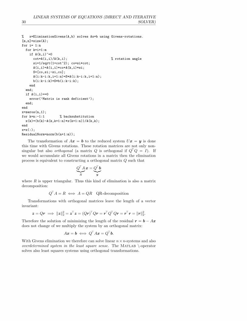
30LINEAR SYSTEMS OF EQUATIONS (DIRECT AND ITERATIVE
SOLVER)
% x=EliminationGivens(A,b) solves Ax=b using Givens-rotations.
[m,n]=size(A);
for i= 1:n
for k=i+1:m
if A(k,i)~=0
cot=A(i,i)/A(k,i); % rotation angle
si=1/sqrt(1+cot^2); co=si*cot;
A(i,i)=A(i,i)*co+A(k,i)*si;
S=[co,si;-si,co];
A(i:k-i:k,i+1:n)=S*A(i:k-i:k,i+1:n);
b(i:k-i:k)=S*b(i:k-i:k);
end
end;
if A(i,i)==0
error(’Matrix is rank deficient’);
end;
end
x=zeros(n,1);
for k=n:-1:1 % backsubstitution
x(k)=(b(k)-A(k,k+1:n)*x(k+1:n))/A(k,k);
end
x=x(:);
ResidualNorm=norm(b(n+1:m));
The transformation of Ax = b to the reduced system Ux = y is donethis time with Givens rotations. These rotation matrices are not only non-singular but also orthogonal (a matrix Q is orthogonal if Q>Q = I). Ifwe would accumulate all Givens rotations in a matrix then the eliminationprocess is equivalent to constructing a orthogonal matrix Q such that
Q>A︸ ︷︷ ︸R
x = Q>b︸︷︷︸y
where R is upper triangular. Thus this kind of elimination is also a matrixdecomposition:
Q>A = R ⇐⇒ A = QR QR-decomposition
Transformations with orthogonal matrices leave the length of a vectorinvariant:
z = Qr =⇒ ‖z‖22 = z>z = (Qr)>Qr = r>Q>Qr = r>r = ‖r‖22.
Therefore the solution of minimizing the length of the residual r = b − Axdoes not change of we multiply the system by an orthogonal matrix:
Ax = b ⇐⇒ Q>Ax = Q>b.
With Givens elimination we therefore can solve linear n×n-systems and alsooverdetermined system in the least square sense. The Matlab \-operatorsolves also least squares systems using orthogonal transformations.

Iterative Solver for Large Sparse Systems 31
We illustrate this with the following example. We wish to fit a functionof the form
y = at+b
t+ c√t
to the points
t 1 2 3 4 5y 2.1 1.6 1.9 2.5 3.1
Inserting the points we get the linear system1 1 1
2 1/2√
2
3 1/3√
3
4 1/4√
4
5 1/5√
5
abc
=
2.11.61.92.53.1
We get with GivensElimination the same result as with Matlab’s \-operator:
>> CurveFit
x =
1.0040
2.1367
-1.0424
y =
1.0040
2.1367
-1.0424
2.3 Iterative Solver for Large Sparse Systems
The solution of sparse linear systems by iterative methods has become oneof the core application and research areas of high performance computing.The size of systems that are solved routinely has increased tremendously overtime. This is because the discretization of partial differential equations canlead to systems that are arbitrarily large.
Iterative methods for solving linear systems can be divided into the olderclass of stationary iterative methods, and the more modern class of non-stationary methods. The class of stationary iterative methods, the first ofwhich was invented by Gauss, are nowadays rarely used as standalone solvers,although they remain core components of more sophisticated algorithms, suchas multi-grid or domain decomposition methods. They are also importantfor preconditioning the newer class of non-stationary iterative methods, inparticular Krylov subspace methods.

32LINEAR SYSTEMS OF EQUATIONS (DIRECT AND ITERATIVE
SOLVER)
2.3.1 Fixed Point Form
For an iterative method one has to write the linear system in a fixed pointform. This is done by a matrix splitting A = M −N . This splitting inducesan iterative method as follows. Starting with some initial approximation x0,we iterate by solving for xk+1
Mxk+1 = Nxk + b, k = 0, 1, 2, . . . , (2.7)
and hope that xk will converge to the desired solution. This is equivalent toxk+1 = F (xk) where F (x) = M−1Nx+M−1b.
An iterative method is called stationary if it can be expressed in thesimple form (2.7), where neither M nor N depends on the iteration countk. Iteration (2.7) is a single stage iteration, since xk+1 depends only on oneformer iterate xk.
Of course, to obtain an efficient method, the matrix splitting must be suchthat solving linear systems with the matrix M requires fewer operations thanfor the original system. On the other hand, we would like to minimize thenumber of iterations. In the extreme case where we chose M = A, and thusN = 0, we converge in one iteration to the solution. Therefore, the choice ofthe splitting should be such that
• M is a good approximation of A,
• Mx = y is easy and cheap to solve.
The fact that we have two generally conflicting criteria means that a com-promise is usually required.
2.3.2 Residual, Error and the Difference of Iterates
We will write iterative methods based on the splitting A = M − N in thestandard form
Mxk+1 = Nxk + b ⇐⇒ xk+1 = M−1Nxk +M−1b. (2.8)
Definition 2.1. (Iteration Matrix) For any matrix splitting A =M − N with M invertible, the matrix G := M−1N is called the iterationmatrix.
Since
M−1Nxk +M−1b = M−1(M −A)xk +M−1b = xk +M−1(b−Axk),
we can also write the iteration in the correction form
xk+1 = xk +M−1rk, (2.9)

Iterative Solver for Large Sparse Systems 33
where rk = b−Axk is called the residual. The residual is a measure of howgood the approximation xk is. The matrix M is called a preconditioner, sinceby iterating with (2.9), if xk → x∞, then x∞ is solution of the preconditionedsystem
M−1Ax = M−1b.
Subtracting the iteration from the split system,
Mx = Nx+ bMxk+1 = Nxk + b
⇒M(x− xk+1) = N(x− xk),
and introducing the error ek := x−xk, we obtain a recurrence for the error,
Mek+1 = Nek ⇐⇒ ek+1 = M−1Nek. (2.10)
From (2.9), it follows that
b−Axk+1︸ ︷︷ ︸rk+1
= b−Axk︸ ︷︷ ︸rk
−AM−1rk,
and we get a recurrence for the residual vectors,
rk+1 = (I −AM−1)rk = (I −AM−1)kr0. (2.11)
Note that M −A = N , and therefore
I −AM−1 = NM−1 = M(M−1N)M−1,
which shows that the iteration matrices I − AM−1 in (2.11) and M−1N in(2.10) are similar, and thus have the same eigenvalues.
Consider the difference of consecutive iterates,
uk = xk+1 − xk.
Using the iteration (2.8), we get
uk = xk+1 − xk = M−1Nxk +M−1b−M−1Nxk−1 −M−1b= M−1N(xk − xk−1)
= M−1Nuk−1.
Hence the differences between consecutive iterates obey the same recurrenceas the error. Furthermore, from
uk = M−1N(xk − x+ x− xk−1)
= M−1N(−ek + ek−1) = −M−1Nek + ek
= (I −M−1N)ek,

34LINEAR SYSTEMS OF EQUATIONS (DIRECT AND ITERATIVE
SOLVER)
we see that the difference between consecutive iterates and the true error arerelated by
uk = M−1Aek.
Finally, from (2.9) we have Muk = rk, a connection between the differenceof consecutive iterates and the residual. We summarize these results in thefollowing Theorem.
Theorem 2.1. (Error, Residual and Difference of Iterates)For a non-singular matrix A ∈ Rn×n and b ∈ Rn, let x ∈ Rn be the solutionof Ax = b, and let A = M −N be a splitting with M non-singular. Choosex0 and compute the sequence of iterates xk+1 = M−1Nxk + M−1b. Letek := x − xk be the error and rk := b − Axk be the residual at step k, andlet uk := xk+1 −xk be the difference of two consecutive iterates. Then thesevectors can be computed by the recurrences
ek+1 = M−1Nek, (2.12)
uk+1 = M−1Nuk, (2.13)
rk+1 = (I −AM−1)rk = NM−1rk, (2.14)
and we have the relation
Muk = rk = Aek. (2.15)
Equation (2.15) has a simple interpretation. The solution of Ax = b can be
obtained by solving Aek = rk with x = xk + ek. However, we cannot solvesystems with the matrix A directly because we assume that A is too large tobe stored and factored. Therefore we replace the problem by an easier oneand solve Muk = rk, and then iterate using xk+1 = xk + uk.
2.3.3 Convergence Criteria
We turn now to the question of when an iteration converges. From the errorrelation (2.12) we conclude
‖ek+1‖ ≤ ‖M−1N‖ ‖ek‖ ≤ . . . ≤ ‖M−1N‖k+1‖e0‖.
Thus, we have convergence if ‖M−1N‖ < 1. This is a sufficient, but not anecessary, condition for convergence: a triangular matrix R with zero diago-nal may have a norm ‖R‖ > 1, but since R is nilpotent, we have Rk → 0 fork →∞. Therefore we need another property that describes convergence.
Definition 2.2. (Spectral Radius) The spectral radius of a matrixA ∈ Rn×n is
ρ(A) := maxj=1,...,n
|λj(A)|,
where λj(A) denotes the j-th eigenvalue of A.

Iterative Solver for Large Sparse Systems 35
Lemma 2.1. For all induced matrix norms ρ(A) ≤ ‖A‖ holds.Proof. Let (λ,x) be an eigenpair of A. From the eigenvector-eigenvalue
relation Ax = λx, we conclude that
|λ|‖x‖ = ‖λx‖ = ||Ax|| ≤ ‖A‖ ‖x‖.
Now since ‖x‖ 6= 0, we obtain |λ| ≤ ‖A‖, and since this holds for anyeigenvalue λ, we also get ρ(A) := maxj=1...n |λj(A)| ≤ ‖A‖.
Theorem 2.2. (Convergence of Stationary Iterative Methods)Let A ∈ Rn×n be non-singular, A = M−N with M non-singular and b ∈ Rn.The stationary iterative method
Mxk+1 = Nxk + b
converges for any initial vector x0 to the solution x of the linear systemAx = b if and only if ρ(M−1N) < 1.
Proof: see our book.
2.3.4 Convergence Factor and Convergence Rate
Consider again the error recurrence (2.12). By induction, we get
ek = (M−1N)ke0,
and taking norms yields a bound for the error reduction over k steps,
‖ek‖‖e0‖
≤ ‖(M−1N)k‖.
We are interested in knowing how many iterations are needed for the errorreduction to reach some given tolerance ε,
‖ek‖‖e0‖
≤ ‖(M−1N)k‖ < ε,
so let us write the right-hand side as
‖(M−1N)k‖ =(∥∥(M−1N)k
∥∥ 1k
)k< ε.
Taking the logarithm, we get
k >ln(ε)
ln(‖(M−1N)k‖
1k
) . (2.16)
This equation does not seem very useful at first glance, since the number ofnecessary iterations k also appears on the right hand side. However, for largek we can get a good estimate using the following Lemma:

36LINEAR SYSTEMS OF EQUATIONS (DIRECT AND ITERATIVE
SOLVER)
Lemma 2.2. For any matrix G ∈ Rn×n with spectral radius ρ(G) and anyinduced matrix norm, we have
limk→∞
‖Gk‖ 1k = ρ(G).
Proof: see our book.
Definition 2.3. (Convergence Factor) The mean convergence factorof an iteration matrix G over k steps is the number
ρk(G) = ‖Gk‖ 1k . (2.17)
The asymptotic convergence factor is the spectral radius
ρ(G) = limk→∞
ρk(G). (2.18)
Definition 2.4. (Convergence Rate) The mean convergence rate ofan iteration matrix G over k steps is the number
Rk(G) = − ln(‖Gk‖ 1
k
)= − ln(ρk(G)). (2.19)
The asymptotic convergence rate is
R∞(G) = − ln(ρ(G)). (2.20)
We now return to the question of how many iteration steps k are neces-sary until the error reduction reaches a given tolerance ε, or until the errordecreases by a factor δ, with ε = 1/δ. The answer is
k ' − ln ε
R∞(M−1N)=
ln δ
R∞(M−1N).
As an example, suppose ρ(M−1N) = 0.8. Then, to obtain another decimaldigit of the solution, we need to take δ = 10 or ε = 0.1 to get
ln 10
− ln 0.8= 10.31.
Thus, we need about 10 iterations.
2.4 Classical Stationary Iterative Methods
In the following sections we present some classical stationary iterative meth-ods. These classical methods are defined in terms of the matrices obtainedby splitting A into the strictly lower triangular part L, the diagonal partD = diag(A), and the strictly upper triangular part U ,
A = L+D + U.

Classical Stationary Iterative Methods 37
2.4.1 Jacobi
The Jacobi method (or Point-Jacobi method) is based on solving for everyvariable locally, with the other variables frozen at their old values. Oneiteration (or sweep) corresponds to solving for every variable once:
Algorithm 2.1. Point-Jacobi Iteration Step
for i=1:n
tmp(i)=(b(i)-A(i,[1:i-1 i+1:n])*x([1:i-1 i+1:n]))/A(i,i);
end
x=tmp(:);
This corresponds to the splitting A = M −N with
M = D, N = −L− U =⇒ Dxk+1 = −(L+ U)xk + b. (2.21)
A classical convergence result for the Jacobi method is the following:
Theorem 2.3. (Convergence of Jacobi) If the matrix A ∈ Rn×n isstrictly diagonally dominant , i.e.
|aii| >∑j 6=i
|aij | for i = 1, . . . , n, (2.22)
then the Jacobi iteration (2.21) converges.Proof. The iteration matrix of the Jacobi method is GJ = −D−1(L+U),
and with Condition 2.22, we obtain that
||GJ||∞ = maxi=1,...,n
1
|aii|∑j 6=i
|aij | < 1.
Now using Lemma 2.1, we obtain
ρ(GJ) ≤ ||GJ||∞ < 1,
which together with Theorem 2.2 concludes the proof.
2.4.2 Gauss-Seidel
The Gauss-Seidel method is similar to the Jacobi method, except that it usesupdated values as soon as they are available. Thus, in Algorithm 2.1, we justreplace the variable tmp by the column vector x.
Algorithm 2.2. Gauss-Seidel Iteration Step
for i=1:n
x(i)=(b(i)-A(i,[1:i-1 i+1:n])*x([1:i-1 i+1:n]))/A(i,i);
end

38LINEAR SYSTEMS OF EQUATIONS (DIRECT AND ITERATIVE
SOLVER)
This corresponds to the splitting
M = D + L, N = −U ⇒ (D + L)xk+1 = −Uxk + b. (2.23)
Since Gauss-Seidel uses the updated values as soon as they are available, onecan expect that convergence will be faster than with Jacobi.
2.4.3 Successive Over-relaxation (SOR)
The successive over-relaxation method (SOR) is derived from the Gauss-Seidel method by introducing an “extrapolation” parameter ω. The compo-nent xi is computed as for Gauss-Seidel but then averaged with its previousvalue.
Algorithm 2.3. SOR Iteration Step
for i=1:n
x(i)=omega*(b(i)-A(i,[1:i-1 i+1:n])*x([1:i-1 i+1:n]))/...
A(i,i)+(1-omega)*x(i);
end
SOR can also be derived by considering the Gauss-Seidel iteration form
(D + L)x = −Ux+ b. (2.24)
Multiplying (2.24) by ω and adding on both sides the expression (1−ω)Dx,we obtain the SOR iteration
(D + ωL)xk+1 = (−ωU + (1− ω)D)xk + ωb. (2.25)
SOR is therefore based on the splitting
A = M −N with M =1
ωD + L and N = −U +
(1
ω− 1
)D, (2.26)
where we divided (2.25) by ω in order to remove the factor ω in front of theright hand side term b and obtain the stationary iterative method in standardform. Notice that for ω = 1 we get as special case the Gauss-Seidel method.
We first show that one cannot choose the relaxation parameter arbitrarilyif one wants to obtain a convergent method. This general, very elegant resultis due to Kahan from his PhD thesis.
Theorem 2.4. (Kahan (1958)) Let A ∈ Rn×n and A = L+D+U withD invertible. If
GSOR = (D + ωL)−1(−ωU + (1− ω)D) (2.27)

Classical Stationary Iterative Methods 39
is the SOR iteration matrix, then the inequality
ρ(GSOR) ≥ |ω − 1| (2.28)
holds for all ω ∈ R.Proof. The key idea is to insert DD−1 between the factors of GSOR,
GSOR = (D + ωL)−1DD−1(−ωU + (1− ω)D)
= (I + ωD−1L)−1(−ωD−1U + (1− ω)I).
Now the determinant of (I +ωD−1L) equals 1, since this matrix is lower tri-angular with unit diagonal, which implies that the determinant of its inversealso equals 1. Therefore
det(GSOR) = det(−ωD−1U + (1− ω)I) = (1− ω)n,
since this second factor is upper triangular with 1− ω on the diagonal. Thedeterminant of a matrix is equal to the product of its eigenvalues, which inour case yields
n∏j=1
λj(GSOR) = (1−ω)n =⇒ |1−ω|n ≤(
maxj|λj(GSOR)|
)n= ρ(GSOR)n,
and this implies the result after taking the n-th root.
From this elegant result, we can conclude that
ρ(GSOR) < 1 =⇒ 0 < ω < 2,
and thus for convergence of SOR it is necessary to choose 0 < ω < 2.The next result is a general convergence result for SOR for a restricted
class of matrices, and does not answer the question yet on how to choose ωin order to obtain a fast method.
Theorem 2.5. (Ostrowski-Reich (1954/1949)) Let A ∈ Rn×n besymmetric and invertible, with positive diagonal elements, D > 0. ThenSOR converges for all 0 < ω < 2 if and only if A is positive definite.
Proof: see our book.An important question, which remained unanswered so far, is how to
choose the parameter ω in SOR in order to obtain a fast method. Thepioneer in this area was David Young, who answered this question for a largeclass of matrices in his PhD thesis1.
Definition 2.5. (Property A) A matrix A ∈ Rn×n has Property A, ifthere exists a permutation matrix P such that
P>AP =
(D1 FE D2
), with D1 and D2 diagonal.
1An electronic version is available at http://www.ma.utexas.edu/CNA/DMY/

40LINEAR SYSTEMS OF EQUATIONS (DIRECT AND ITERATIVE
SOLVER)
Example 2.1. If we discretize the one-dimensional Laplacian ∂2
∂x2 byfinite differences on a regular grid, the discrete operator becomes
A =1
h2
−2 11 −2 1
1. . .
. . .
. . .. . . 11 −2
∈ Rn×n.
If n is even, then A can be permuted as required for Property A,
P>AP =
−2 1. . . 1
. . .
. . .. . .
. . .
−2 1 11 1 −2
. . .. . .
. . .
. . . 1. . .
1 −2
,
with P constructed by the unit vectors ej as follows:
P = [e1, e3, . . . en−1, e2, e4, . . . , en].
Theorem 2.6. (Optimal SOR Parameter (Young 1950)) Let A ∈Rn×n have Property A, and let
A = P>AP =
[D1 FE D2
]= L+D + U,
with all diagonal elements of D1 and D2 nonzero. Let
GSOR = (D + ωL)−1(−ωU + (1− ω)D)
be the SOR iteration matrix for A and
GJ = −D−1(L+ U)
the Jacobi iteration matrix. If the eigenvalues µ(GJ) are real and ρ(GJ) < 1,then the optimal SOR parameter ω for A is
ωopt =2
1 +√
1− ρ(GJ)2.

Classical Stationary Iterative Methods 41
Proof: see our book.For ωopt, the optimized convergence factor of SOR becomes
ρ(GSOR)min = ωopt − 1 =
(ρ(GJ)
1 +√
1− ρ(GJ)2
)2
=1−
√1− ρ(GJ)2
1 +√
1− ρ(GJ)2.
(2.29)In general, we do not know in advance the spectral radius ρ(GJ), so we
cannot compute ωopt for SOR and have to rely on estimates. The rule ofthumb is to try to overestimate ω, because of the steeper slope on the left.To illustrate this, we consider the function
Algorithm 2.4. SOR Spectral Radius
function r=Rho(omega,mu);
% RHO computes spectral radius for SOR
% r=Rho(omega,mu) computes the spectral radius of the iteration
% matrix for SOR, given the spectral radius mu of the Jacobi
% iteration matrix and the relaxation parameter omega
if omega<2/(1+sqrt(1-mu^2))
r=((omega*mu)^2-2*(omega-1)+sqrt((omega*mu)^2*...
((omega*mu)^2-4*(omega-1))))/2;
else
r=abs(omega-1);
end;
and plot it for various values of µ using the commands
axis([0,2,0,1])
hold on
xx=[0:0.01:2];
for mu=0.1:0.1:0.9
yy=[];
for x=xx
yy=[yy Rho(x,mu)];
end
plot(xx,yy)
end
We can see that for µ = 0.9, the choice of ω ≈ 1.4 yields a convergence factorof about 0.4. This is a drastic improvement over Jacobi, leading to about 8to 9 times fewer iterations, since µ8.5 ≈ 0.4.
The optimal choice of the relaxation parameter ω also improves the con-vergence factor asymptotically: one gains a square root, as one can see whensetting ρ(GJ) = 1 − ε, and then expanding the corresponding optimizedρ(GSOR) for small ε. Using the Maple commands
rho:=mu^2/(1+sqrt(1-mu^2))^2;

42LINEAR SYSTEMS OF EQUATIONS (DIRECT AND ITERATIVE
SOLVER)
Figure 2.1.ρ(GSOR) as function of ω for µ = 0.1 : 0.1 : 0.9
mu:=1-epsilon;
series(rho,epsilon,1);
we obtain ρ(GSOR) = 1 − 2√
2ε + O(ε), which shows that indeed the im-provement is a square root.
2.4.4 Richardson
In order to explain the Richardson iteration, we consider the correction form(2.9) of the stationary iterative method,
xk+1 = xk +M−1rk.
If we choose M−1 = αI, which corresponds to the splitting M = 1αI and
N = 1αI −A, we obtain the Method of Richardson
xk+1 = xk + α(b−Axk) = (I − αA)xk + αb. (2.30)
Theorem 2.7. (Convergence of Richardson) Let A ∈ Rn×n be sym-metric and positive definite. Then
a) Richardson converges if and only if 0 < α < 2ρ(A)
.
b) Convergence is optimal for αopt =2
λmax(A) + λmin(A).
c) The asymptotic convergence factor is
ρ(I − αoptA) =κ(A)− 1κ(A) + 1
, where κ(A) :=λmax(A)λmin(A)
.

Nonstationary Iterative Methods 43
2.5 Nonstationary Iterative Methods
In contrast to the stationary iterative methods, the increment xk+1 − xkchosen by non-stationary iterative methods varies from one iteration to thenext. We assume throughout this section that the matrix A ∈ Rn×n symmet-ric is positive definite. To start, we consider the method of Richardson in itsoriginal form, where the parameter α is allowed to change in each iteration,
xk+1 = xk + αk(b−Axk). (2.31)
We consider for µ ∈ R the norm (it is a norm since A is positive definite)
‖r‖2A−µ = r>A−µr, (2.32)
and using Ritz’s idea2, we want to determine the value of αk that minimizes
Q(αk) := ‖rk+1‖2A−µ . (2.33)
Differentiating with respect to αk and noting that iteration (2.31) can bewritten as a recurrence for residuals,
rk+1 = (I − αkA)rk, (2.34)
we get
dQ
dαk= 0 = 2r>k+1A
−µ d
dαkrk+1 = 2((I − αkA)rk)>A−µ(−Ark).
Solving for αk, we obtain
αk =r>kA
1−µrkr>kA
2−µrk. (2.35)
Useful choices for µ are 0 and 1, since otherwise we would have to solveequations with the matrix A, or perform more than one multiplication withA in order to determine αk.
2.5.1 Conjugate Residuals
For µ = 0, (2.35) gives
αk =r>kArk‖Ark‖22
, (2.36)
so in this case we are minimizing locally
‖rk+1‖22 = ‖Aek+1‖22 = ‖ek+1‖2A2 −→ min .
2It was Ritz who first proposed in 1908 to find approximate solutions to minimizationproblems by searching in a small, well chosen subspace.

44LINEAR SYSTEMS OF EQUATIONS (DIRECT AND ITERATIVE
SOLVER)
Using (2.34) for rk+1 and (2.36) for αk, a short calculation shows that
r>k+1Ark = 0,
which means that the residuals are conjugate, and therefore this method iscalled the conjugate residuals algorithm.
Algorithm 2.5. Conjugate Residuals Algorithm
k = 0; x = x0 ;r = b−Ax;while not converged
k = k + 1;ar = Ar;
α =r>ar‖ar‖2
;
x = x+ αr;
r = r − αar;end
2.5.2 Steepest Descent
Another method, called the Steepest Descent method, can be derived by choos-ing µ = 1; then (2.35) gives
αk =‖rk‖2
r>kArk. (2.37)
Theorem 2.8. (Steepest Descent Properties) Let A ∈ Rn×n besymmetric and positive definite. With the choice of αk given by (2.37), thefollowing functionals are being minimized by the method (2.31):
a) ‖rk+1‖2A−1 = r>k+1A−1rk+1.
b) Q(xk + αrk) as a function of α, where Q(x) = 12x>Ax− b>x.
c) ‖ek+1‖2A = e>k+1Aek+1.
The pairs of consecutive residuals obtained by the this method of steepestdescent are not conjugate but orthogonal, as one can see by a short calculationevaluating the scalar product r>k+1rk.
Algorithm 2.6. Steepest Descent Algorithm
k = 0; x = x0 ;r = b−Ax;

Nonstationary Iterative Methods 45
while not converged
k = k + 1;ar = Ar;
α =r>r
r>ar;
x = x+ αr;
r = r − αar;end
Theorem 2.9. (Steepest Descent Convergence) Let A ∈ Rn×n besymmetric and positive definite. Then the method of steepest descent con-verges.
2.5.3 The Conjugate Gradient Method
The Conjugate Gradient Method (CG) is a method to solve linear systems ofequations with symmetric and positive definite coefficient matrices. The pre-conditioned conjugate gradient method is today used as a standard methodin many software libraries, and CG is the starting point of Krylov methodswhich are listed among the top ten algorithms of the last century.
Let A ∈ Rn×n be a symmetric positive definite matrix. Then solving thelinear system Ax = b is equivalent to finding the minimum of the quadraticform
Q(x) =1
2x>Ax− x>b, (2.38)
as one can see by differentiation. The conjugate gradient method belongs tothe class of descent methods. Such methods compute the minimum of thequadratic form (2.38) iteratively: at step k,
1. a direction vector pk is chosen, and
2. the new vector xk+1 = xk+αkpk is computed, where αk is chosen suchthat
Q(xk + αkpk) −→ min .
An interesting class of methods is obtained if we choose conjugate directions,that is if
p>i Apj = 0, for i 6= j. (2.39)
Conjugate directions have the following properties:
Theorem 2.10. Let A ∈ Rn×n be a symmetric positive definite matrix,let x0 ∈ Rn be given, and let the direction vectors pi 6= 0, i = 0, 1, . . . , n− 1be conjugate. Then the sequence xk defined by
xk+1 = xk + αkpk, with αk =p>krkp>kApk
and rk = b−Axk

46LINEAR SYSTEMS OF EQUATIONS (DIRECT AND ITERATIVE
SOLVER)
converges in at most n steps to the solution of Ax = b.Proof. Let xk+1 = xk + αp. Then minimizing
Q(xk+1) =1
2x>k+1Axk+1 − b>xk+1
with respect to α yields the equation
∂Q
∂α= p>Axk+1 − b>p = p>A(xk + αp)− b>p = 0,
and we get the solution
α =p>rkp>Ap
.
Thus, by this choice of α, we are minimizing the quadratic form Q along theline xk + αp.
Before continuing the proof for the general case, we first look at the casewhere the matrix A is diagonal, which will be helpful later. In that case wehave
Q(x) =1
2
∑i
aiix2i − b
>x,
and as conjugate direction we can take the unit vectors ei, since e>i Aej =aij = 0 for i 6= j. In this special case, Q is minimal for xi = bi/aii. Now letx0 be some initial vector. Then
x1 = x0 + α0e1 with α0 =e>1 (b−Ax0)
e>1Ae1=b1 − a11x0,1
a11.
Thus, in the first iteration step, only the first element of the initial vector ischanged and we obtain
x1 =
b1a11x0,2
...x0,n
.
In the second iteration step, we obtain
x2 =
b1a11b2a22x0,3
...x0,n
,
and so on, so after n steps we do get the exact solution xn = x.Now let A be a general symmetric positive definite matrix, and P =
[p0, . . . ,pn−1] be the conjugate directions. Then P>AP = D with D diagonal

Nonstationary Iterative Methods 47
with dii = p>i Api > 0 (note this is not the eigenvalue decomposition, sinceP is not orthogonal!). With the change of variables, x = Py we get
Q(x) =1
2(Py)>APy − b>Py =
1
2y>Dy − (P>b)>y =: R(y).
Minimizing this quadratic form with respect to y is equivalent to solving thediagonal linear system Dy = P>b. Using the unit vectors ei as conjugatedirections, we see that the coefficients are
αk =e>k(P>b−Dyk)
e>kDek=p>k(b−Axk)
p>kApk,
and thus they are the same as for the original variable x. As shown beforein the special case, the iteration
yk+1 = yk + αkek (2.40)
converges in n steps. Multiplying (2.40) from the left by P , we see that
xk+1 = xk + αkpk
also converges in n steps, which concludes the proof.
The previous theorem shows that conjugate directions can be used toconstruct an iterative method that converges in a finite number of steps. Asa result, we are interested in finding conjugate directions for a given matrixA. One possibility is to use the eigenvectors of A: if
AQ = QD, Q>Q = I,D = diag(λ1, . . . , λn)
is the eigen-decomposition of A, then the eigenvectors Q are conjugate:
Q>AQ = D.
However, computing the eigen-decomposition is too expensive for our pur-pose, as it is more expensive than solving the linear system. Stiefel andHestenes found a much more efficient algorithm to construct such directions,now known as the conjugate gradient algorithm:
Algorithm 2.7. Conjugate Gradient Algorithm: CGHS
choose x0, p0 = r0 := b−Ax0; ;for k = 0 : n− 1
αk =r>kpkp>kApk
; (2.41)
xk+1 = xk + αkpk; (2.42)
rk+1 = rk − αkApk; (2.43)
βk =p>kArk+1
p>kApk; (2.44)
pk+1 = rk+1 + βkpk; (2.45)
end

48LINEAR SYSTEMS OF EQUATIONS (DIRECT AND ITERATIVE
SOLVER)
Theorem 2.11. Let A ∈ Rn×n be symmetric and positive definite. Thenthe direction vectors pj in Algorithm 2.7 are conjugate, and pj 6= 0 if xj isnot the exact solution. Furthermore the residual vectors rj are orthogonal:r>j ri = 0 for i 6= j and ri ⊥ pj , i > j.
Proof: see our bokk.In Algorithm 2.7, each iteration seemingly requires two matrix-vector
multiplications, Apk and Ark+1. However, it is possible to avoid the secondone as follows. Using Statements (2.43) and (2.45), we get, because of theconjugacy and the orthogonality,
r>k+1pk+1 = (rk − αkApk)>pk+1 = r>kpk+1 = r>k(rk+1 + βkpk) = βkr>kpk.
Solving for βk, and using again Statement (2.45) and that the residuals areorthogonal to the direction vectors, we get
βk =r>k+1pk+1
r>kpk=r>k+1(rk+1 + βkpk)
r>k(rk + βk−1pk−1)=‖rk+1‖2
‖rk‖2.
Because of r>kpk = ‖rk‖2 the computation of αk simplifies also to
αk =‖rk‖2
p>kApk. (2.46)
With these observations, we obtain a version of CG which uses only onematrix-vector multiplication per iteration step:
Algorithm 2.8. Conjugate Gradients
function [X,R,P,alpha,beta]=CG(A,b,x0,m);
% CG conjugate gradient method
% [X,R,P,alpha,beta]=CG(A,b,x0,n) computes an approximation for the
% solution of the linear system Ax=b performing m steps of the
% conjugate gradient method starting with x0, and returns in the
% matrix X the iterates, in the matrix R the residuals, in P the
% conjugate directions and the coefficients alpha and beta.
x=x0; r=b-A*x; p=r;
R=r; P=p; X=x;
oldrho =r’*r;
for k=1:m
Ap = A*p;
alpha(k) = oldrho/(p’*Ap);
x = x+alpha(k)*p;
r = r-alpha(k)*Ap;
rho= r’*r;
beta(k) = rho/oldrho;

Nonstationary Iterative Methods 49
oldrho=rho;
p = r+beta(k)*p;
X = [X,x];
R = [R,r];
P = [P,p];
end
Theorem 2.12. For the vectors generated by the Conjugate GradientAlgorithm 2.7, we have for i = 0, 1, 2, . . .
Api ∈ spanp0, . . . ,pi+1, (2.47)
ri ∈ spanp0, . . . ,pi = Ki+1(A,p0) = Ki+1(A, r0). (2.48)
The proof is by induction, see our book.
The convergence analysis of CG is most naturally performed in a normassociated to the system matrix: let A ∈ Rn×n be a symmetric (A> = A) andpositive definite (x>Ax > 0,∀x 6= 0) matrix. Then one can define a vectornorm associated with A, the so called A-norm or energy norm,
‖x‖A :=√x>Ax.
Theorem 2.13. (Optimality of CG) Let x be the solution of Ax =b, with A ∈ Rn×n symmetric and positive definite. Then, for each k, theapproximation xk+1 obtained by CG minimizes the A-norm of the error,
‖x− xk+1‖A = minx∈Sk
‖x− x‖A,
where the affine Krylov subspace Sk is defined by
Sk = x0 +Kk+1(A, r0).
Proof: see our book.
We are now ready to give a different interpretation of Theorem 2.13. Sincewe chose p0 = r0, the approximation xk ∈ Sk−1 is
xk = x0 +
k−1∑j=0
cjAjr0.
Hence it follows that
rk = b−Axk = r0 −k−1∑j=0
cjAj+1r0 = Rk(A)r0

50LINEAR SYSTEMS OF EQUATIONS (DIRECT AND ITERATIVE
SOLVER)
where the polynomial Rk with Rk(0) = 1 is the residual polynomial. UsingEquation (2.15), A−1rk = x− xk, we can write
‖x− xk‖2A = r>kA−1AA−1rk = r>kA
−1rk = ‖Rk(A)r0‖2A−1 .
Note that since A is symmetric and positive definite, A−1 is also symmetricand positive definite, so it can be used to define a norm as well. Theorem2.13 now becomes
Theorem 2.14. Let xk be the approximation obtained by CG at the k-thstep. Let Rk be a polynomial of degree k with Rk(0) = 1. Then
‖ek‖A = ‖x− xk‖A = minRk(0)=1
‖Rk(A)r0‖A−1 .
As an immediate corollary, we have
Corollary 2.1. If A has only m ≤ n different eigenvalues, then CGconverges in at most m steps.
Proof. This theorem follows immediately from Theorem 2.14 since theminimal polynomial for A has degree m.
The advantage of CG is that no parameters have to be estimated. Inaddition, CG finds the best polynomial for the given spectrum of A, whichexplains why in practice the CG algorithm converges better if the eigenvaluesare clustered.
Let us derive a general error estimate. Here, it is impossible to takeinto account all the various spectra possible, so we again assume that thespectrum of A is contained in an interval and use Chebyshev polynomials.Using the eigen-decomposition
A = QDQ>, Q>Q = I, D = diag(λ1, . . . , λn),
we obtain‖Rk(A)r0‖2A−1 = r>0QRk(D)2D−1Q>r0.
Let t := Q>r0, then
‖Rk(A)r0‖2A−1 = t>Rk(D)2D−1t =
n∑i=1
t2iRk(λi)
2
λi
≤ maxiRk(λi)
2n∑i=1
t2iλi.
Now with r0 = A(x− x0) we observe that
n∑i=1
t2iλi
= r>0Q>D−1Qr0 = r>0A
−1r0
= (x− x0)>A(x− x0)
= ‖x− x0‖2A = ‖e0‖2A.

Nonstationary Iterative Methods 51
Assume that 0 < a = λ1 ≤ λ2 ≤ · · · ≤ λn = b, then
maxiRk(λi)
2 ≤ maxa≤λ≤b
|Rk(λ)|2.
Using the properties of Chebychev-polynomials (see our book)
minRk(0)=1
maxa≤λ≤b
|Rk(λ)| = 1∣∣∣Ck (a+ba−b
)∣∣∣ ≤ 2
(√κ− 1√κ+ 1
)k,
together with Theorem 2.14, we get:
Theorem 2.15. (Convergence Estimate for CG) Let xk be theapproximation at the k-th step of the CG algorithm. Then the error ek :=x− xk satisfies the estimate
‖ek‖A ≤ 2
(√κ− 1√κ+ 1
)k‖e0‖A,
where κ = λn/λ1 is the condition number of the matrix A.
The Rayleigh quotient is bounded by the extremal eigenvalues, so that
λ1 ≤x>Ax
x>x=‖x‖2A‖x‖22
≤ λn =⇒√λ1‖x‖2 ≤ ‖x‖A ≤
√λn‖x‖2.
From this inequality, we get the error estimate of Theorem 2.15 in the 2-norm,
‖ek‖2 ≤ 2
(√κ− 1√κ+ 1
)k√κ‖e0‖2. (2.49)
This error estimate does not necessarily imply that the error decreases mono-tonically in each step, it is just an upper bound. However, we also have thefollowing result:
Theorem 2.16. (Monotonicity of CG) With each CG step, the errordecreases. More specifically, if xk−1 6= x, then
‖x− xk‖2 < ‖x− xk−1‖2.
2.5.4 Arnoldi Process
The conjugate gradient methods solves large linear systems with a symmetricpositive definite coefficient matrix. The Arnoldi process is used for non-symmetric matrices.
The Arnoldi process constructs an orthogonal basis of the Krylov space
Kk(A, r0) = spanr0, Ar0, A2r0, . . . , Ak−1r0

52LINEAR SYSTEMS OF EQUATIONS (DIRECT AND ITERATIVE
SOLVER)
using Gram-Schmidt orthogonalization. It computes the QR decompositionof the matrix Kk ∈ Rn×k,
Kk := [r0, Ar0, . . . , Ak−1r0] = QkRk, (2.50)
with Qk ∈ Rn×k orthogonal and Rk ∈ Rk×k upper triangular. In the j-thstep the vector Ajr0 is orthonormalized to produce qj+1. This is done usingthe Gram-Schmidt process, by first computing the projections on the vectorsq1, . . . , qj which have already been constructed,
ri,j+1 = q>i Ajr0, i = 1, . . . , j.
Then the corresponding components are subtracted,
u = Ajr0 −j∑i=1
ri,j+1qi, (2.51)
and the result is normalized
rj+1,j+1 = ‖u‖, qj+1 =1
rj+1,j+1u. (2.52)
Idea of Arnoldi: If we are only interested in the orthogonal basis definedby the matrix Qk, then we can replace the vector Ajr0 by Aqj . This isjustified because as long as the Krylov matrix Kk has full rank, it followsfrom Kk = QkRk that Qk = KkR
−1k , and thus with α = R−1k ej , we obtain
qj = α0r0 + α1Ar0 + · · ·+ αj−1Aj−1r0, with αj−1 =
1
rj,j6= 0.
So qj contains a component which points into the direction Aj−1r0, and
therefore Aqj can be used instead of Ajr0. With this modification, theorthogonalization step becomes
hj+1,jqj+1 = Aqj −j∑i=1
hijqi, (2.53)
where hij = q>i Aqj are the projections and hj+1,j is the normalizing factor.Note that we could have obtained a similar relation by inserting the rela-
tion qj+1 = u/rj+1,j+1 (cf. (2.52)) into (2.51):
rj+1,j+1qj+1 = Ajr0 −j∑i=1
ri,j+1qi, (2.54)
Comparing (2.53) with (2.54), we see that we have shifted the secondindex in hij by one relative to the rij . The reason is that we want to write(2.53) now in matrix form as
Aqj =
j+1∑i=1
hijqi, j = 1, . . . , k, (2.55)

Nonstationary Iterative Methods 53
where the first vector q1 no longer appears on the left hand side. Using thematrices Qk = [q1, . . . , qk] ∈ Rn×k and
Hk =
h11 h12 · · · h1kh21 h22 · · · h2k
. . .. . .
.... . . hk,k
hk+1,k
∈ R(k+1)×k,
(2.55) can now be written as
AQk = Qk+1Hk.
If we define the upper Hessenberg matrix Hk ∈ Rk×k to contain the firstk rows of Hk, then, after k < n steps of the Arnoldi process, we have theequation
AQk = QkHk + hk+1,kqk+1e>k . (2.56)
Since the column vectors qj of Qk are orthogonal, it follows from Equation(2.56) that also
Q>jAQj = Hj , j = 1, . . . , k. (2.57)
The matrices Hj are often called the projections of the matrix A onto theKrylov subspace. It can happen that for some k we get hk+1,kqk+1 = 0. Inthis case, AQk = QkHk holds, which means we have computed an invariantsubspace spanned by the columns of Qk; this event is therefore called a “luckybreakdown”. If λ and x is an eigenpair of Hk then λ and y = Qkx is aneigenpair of A.
Especially for k = n we have qn+1 = 0, and thus
AQn = QnHn ⇐⇒ Q>nAQn = Hn,
which means that A has been transformed by an orthogonal similarity trans-formation to upper Hessenberg form. This is usually done as shown in thebook by using elementary orthogonal matrices. The Arnoldi process is an-other way of computing this transformation, but it is less stable numericallybecause it uses a Gram-Schmidt process. Using the more stable modifiedGram-Schmidt process (see book), we get the algorithm
Algorithm 2.9.Arnoldi algorithm to compute A = QTQ>
function [H,Q,v]=Arnoldi(A,r,k);
% ARNOLDI Arnoldi process
% [H,Q,v]=Arnoldi(A,r,k) applies k<=n steps of the Arnoldi process to
% the matrix A starting with the vector r. Computes Q orthogonal and

54LINEAR SYSTEMS OF EQUATIONS (DIRECT AND ITERATIVE
SOLVER)
% H upper Hessenberg such that AQ=QH+ve_k^T, with Q(:,1)=r/norm(r).
ninf=norm(A,inf);
Q(:,1)=r/norm(r);
for j=1:k
v=A*Q(:,j);
for i = 1:j
H(i,j)=Q(:,i)’*v;
v=v-H(i,j)*Q(:,i);
end
if j<k
H(j+1,j)=norm(v);
if abs(H(j+1,j))+ninf==ninf
disp(’lucky breakdown occured!’);
H=H(1:end-1,:);
break;
end
Q(:,j+1)=v/H(j+1,j);
end
end
As an example, we consider for n = 4 the magic square matrix fromMatlab:
>> A=magic(4);
>> r=(1:4)’;
>> [H,Q,v]=Arnoldi(A,r,4)
H =
28.3333 13.2567 -4.1306 -1.3734
12.7550 3.7347 12.9021 3.9661
0 3.8955 -2.2508 1.9173
0 0 9.9142 4.1827
Q =
0.1826 0.7539 0.4895 0.3984
0.3651 0.4628 -0.2153 -0.7785
0.5477 0.0573 -0.6830 0.4798
0.7303 -0.4628 0.4975 -0.0702
v =
1.0e-15 *
-0.2220
0.8882
0.4441
-0.1110
>> norm(A*Q-Q*H)
ans =
2.0368e-15
If we start however with a vector of all ones, we obtain
>> r=ones(4,1);

Nonstationary Iterative Methods 55
>> [H,Q,v]=Arnoldi(A,r,3)
lucky breakdown occured!
H =
34
Q =
0.5000
0.5000
0.5000
0.5000
v =
0
0
0
0
and Arnoldi found that the vector of all ones is an eigenspace, as expectedfor a magic square.
2.5.5 Solving Linear Equations with Arnoldi
We consider the linear system Ax = b. Let x0 be an initial approximation tothe solution and r0 = b − Ax0 the corresponding residual. After k Arnoldisteps, we have the matrix Qk whose column vectors form an orthogonal basisof the Krylov subspace Kk(A, r0). For an approximate solution, we make theansatz
xk = x0 +Qky. (2.58)
One way to determine the vector y is to impose a Galerkin condition and torequire the residual rk = b− Axk to be orthogonal to the Krylov subspace.This method is known under the name of Full Orthogonalization Method orFOM. Requiring orthogonality means
rk ⊥ Kk(A, r0)
⇐⇒ 0 = Q>krk = Q>k(b−Axk)
= Q>k(b−Ax0 −AQky) = Q>k(r0 −AQky)
⇐⇒ Q>kAQky = Q>kr0.
Using (2.56) and Q>kr0 = ‖r0‖e1, which is true since q1 = r0
‖r0‖ and q>j q1 = 0,
j > 1, we obtainHky = ‖r0‖e1. (2.59)
Thus, we have to solve this small k × k linear system with the Hessenbergmatrix Hk to get the approximation xk = x0 +Qky.
The approximation xk may be computed after each Arnoldi step. But fora large system, one might want to do so only every once in a while. Notethat the new residual is an element of the next Krylov space, since
xk = x0 +Qky =⇒ rk = b−Axk = r0 −AQky ∈ Kk+1(A, r0). (2.60)

56LINEAR SYSTEMS OF EQUATIONS (DIRECT AND ITERATIVE
SOLVER)
Furthermore,
rk = r0 −AQky = r0 −Qk+1Hky
= r0 −QkHky − hk+1,kqk+1yk
= Qk (‖r0‖e1 −Hky)︸ ︷︷ ︸0
−hk+1,kqk+1yk,
which shows that rk and qk+1 are collinear.In the following algorithm, we compute the new solution in each iteration
step.
Algorithm 2.10. FOM for Solving Linear Systems
function [X,R,H,Q]=FOM(A,b,x0);
% FOM full orthogonalization method
% [X,R,H,Q]=FOM(A,b,x0) computes the decomposition A=QHQ’,
% Q orthogonal and H upper Hessenberg, Q(:,1)=r/norm(r),
% using Arnoldi in order to solve the system Ax=b with the
% full orthogonalization method. X contains the iterates
% and R the residuals
n=length(A); X=x0;
r=b-A*x0; R=r; r0norm=norm(r);
Q(:,1)=r/r0norm;
for k=1:n
v =A*Q(:,k);
for j=1:k
H(j,k)=Q(:,j)’*v; v=v-H(j,k)*Q(:,j);
end
e0=zeros(k,1); e0(1)=r0norm; % solve system
y=H\e0; x= x0+Q*y;
X=[X x];
R=[R b-A*x];
if k<n
H(k+1,k)=norm(v); Q(:,k+1)=v/H(k+1,k);
end
end
Example:
A=[ 0 -4 -8 -2
-4 -7 -7 -8
-9 -5 -4 -5
0 -5 -9 -6 ]
n=length(A); x=(1:n)’; b=A*x;
x0=x-5; % Starting vector
[X,R,H,Q]=FOM(A,b,x0)
Q’*A*Q % Check Q’*A*Q = H

Problems 57
>> demoFOM
A =
0 -4 -8 -2
-4 -7 -7 -8
-9 -5 -4 -5
0 -5 -9 -6
X =
-4.0000 -0.7314 0.2662 1.0638 1.0000
-3.0000 3.0703 3.1914 1.6232 2.0000
-2.0000 3.3698 1.8713 3.1228 3.0000
-1.0000 3.6694 4.6950 4.1728 4.0000
R =
-70.0000 6.5787 -2.8739 -0.1797 0.0000
-130.0000 0.5106 3.0638 -0.1411 0.0000
-115.0000 -10.4047 -1.6869 0.0451 0.0000
-100.0000 6.6965 -0.0313 0.2573 0.0000
H =
-21.4159 -0.7691 2.4745 -1.8287
1.4153 6.8119 2.7029 4.0318
0 2.1826 -1.3041 -1.6275
0 0 0.1709 -1.0919
Q =
-0.3299 0.4691 0.6349 0.5177
-0.6127 0.0364 -0.6768 0.4065
-0.5420 -0.7420 0.3726 -0.1299
-0.4713 0.4775 0.0069 -0.7415
ans =
-21.4159 -0.7691 2.4745 -1.8287
1.4153 6.8119 2.7029 4.0318
-0.0000 2.1826 -1.3041 -1.6275
-0.0000 -0.0000 0.1709 -1.0919
2.6 Problems
1. Write a function x=forwards(L,b) to solve the system Lx = b withthe lower diagonal matrix L by forward substitution using the SAXPYvariant.
2. Consider the linear system Ax = b with
A =
1 2 −2 −6−3 −1 −2 α−4 3 9 16
5 7 −6 −15
b =
1111
.
The element a24 = α has been lost. Assume, however, that before whenα was available, the solution with Matlab turned out to be
> x=A\b

58LINEAR SYSTEMS OF EQUATIONS (DIRECT AND ITERATIVE
SOLVER)
x =
1.0e+15 *
0.7993
-0.3997
1.1990
-0.3997
Can you determine with this information the missing integer matrixelement α = a24?
3. Use the function EliminationGivens to investigate if the two lines gand h intersect. If they don’t intersect, compute their distance.
g : x =
122
+ r
131
, h : x =
3−72
+ s
3−1−3
,
4. Consider the linear system of equations Ax = b with the matrix
A =
2 −1
−1 2. . .
. . .. . . −1−1 2
(2.61)
and choose b such that the exact solution is the vector [1:n].
Write an experimental program for n = 1000 using first the Jacobimethod. Perform 100 Jacobi iteration steps and estimate the spectralradius using uk+1 = M−1Nuk and ρ ≈ ‖uk+1‖/‖uk‖.Compare the estimated spectral radius to the true one.
Then compute with the estimated spectral radius according to the the-ory of David Young the optimal over-relaxation parameter ω and con-tinue for 100 more iteration steps with SOR.
Compute in each step the true error ek = x−xk and store its norm ina vector. Finally use semilogy and plot the error norm as a function ofthe iteration steps. You should notice a better convergence with SOR.
5. Solve the same system using the conjugate gradient method. Modifyour function CG such that the norm of the error is stored for every step.For this you need to add the exact solution to the input parameter list.
[x,Errors]=conjgradient(A,b,x0,xexact,m);
(a) Apply 200 steps of CG and plot the norm of the errors and compareit to SOR.

Problems 59
(b) Plot the error and the residuals for m = 1000
6. A linear system with the matrix (2.61) could be preconditioned withthe matrix
M =
1 −1
−1 2. . .
. . .. . . −1−1 2
= FF> with F =
1
−1 1. . .
. . .. . .
−1 1
Suppose you are solving the preconditioned system F−1AF−>(F>x) =F−1b with CG. How many iteration steps are at most necessary? Jus-tify your claim by applying Corollary2.1.

60LINEAR SYSTEMS OF EQUATIONS (DIRECT AND ITERATIVE
SOLVER)

Chapter 3. Nonlinear Equations
3.1 Bisection
Consider the following problem: We are given the area F = 12 of a right-angled triangle and the section p = 2 of the hypotenuse (see Figure 3.1).Compute the edges of the triangle.
SSSSSSS
F
q p
hc
Figure 3.1. Triangle Problem
Denote with q the second section of the hypotenuse so that c = p + q. Theheight theorem says h2c = pq. Replacing c and hc in the expression for thearea F = 1
2chc we get
F =p+ q
2
√pq
which is an interesting relation since it says that the area of the triangle isequal to the product of the arithmetic and the geometric mean of the twosections of the hypotenuse. Inserting the numerical values we get an equationfor x = q:
f(x) =2 + x
2
√2x− 12 = 0.
We wish to find a value x such that f(x) = 0. It is easy to see that f(0) = −12and f(8) = 8, so we conclude, since f is a continuous function in (0, 8), thatthere exists a zero in this interval.
It is obvious to try the mid-point of the interval x = 0+82 = 4. We obtain
f(4) = 3√
8 − 12 = −3.5147 and conclude that our solution must be in thesmaller interval (4, 8). Another bisection x = 4+8
2 = 6 gives f(6) = 1.8564thus the solution must be in the interval (4, 6). We can continue this process

62 NONLINEAR EQUATIONS
called bisection until the two bounds are close enough to give us the solutionto the precision we wish to have.
The following function Bisekt can be used for this:
function x=Bisekt(f,a,b)
x=(a+b)/2;
while b-a>1e-5
if f(x)<0,
a=x;
else
b=x;
end
x=(a+b)/2
end
Indeed we get the solution with
>> x=Bisekt(@(x)(2+x)/2*sqrt(2*x)-12,4,6)
x =
5.3423
Note that the function Bisekt must be improved to serve as a more generalroot-finder. We will do that in Problem 1.
3.2 Fixed Point Iteration
Consider the equationf(x) = 0, (3.1)
where f(x) is a real function defined and continuous in the interval [a, b].Assume that s ∈ [a, b] is a zero of f(x). In order to compute s, we transform(3.1) algebraically into fixed point form,
x = F (x), (3.2)
where F is chosen so that F (x) = x ⇐⇒ f(x) = 0. A simple way to do thisis, for example, x = x+f(x) =: F (x), but other choices are possible. Findinga zero of f(x) in [a, b] is then equivalent to finding a fixed point x = F (x) in[a, b]. The fixed point form suggests the fixed point iteration
x0 initial guess, xk+1 = F (xk), k = 0, 1, 2, . . . . (3.3)
The hope is that iteration (3.3) will produce a convergent sequence xk → s.For example, consider
f(x) = xex − 1 = 0. (3.4)
When trying to solve this equation in Maple, we find
solve(x*exp(x)-1,x);
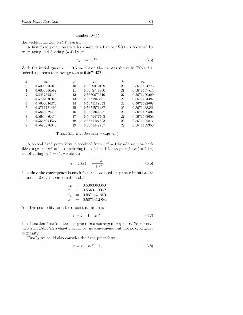
Fixed Point Iteration 63
LambertW(1)
the well-known LambertW function.A first fixed point iteration for computing LambertW(1) is obtained by
rearranging and dividing (3.4) by ex,
xk+1 = e−xk . (3.5)
With the initial guess x0 = 0.5 we obtain the iterates shown in Table 3.1.Indeed xk seems to converge to s = 0.5671432...
k xk k xk k xk0 0.5000000000 10 0.5669072129 20 0.56714247761 0.6065306597 11 0.5672771960 21 0.56714375142 0.5452392119 12 0.5670673519 22 0.56714302903 0.5797030949 13 0.5671863601 23 0.56714343874 0.5600646279 14 0.5671188643 24 0.56714320635 0.5711721490 15 0.5671571437 25 0.56714333816 0.5648629470 16 0.5671354337 26 0.56714326347 0.5684380476 17 0.5671477463 27 0.56714330588 0.5664094527 18 0.5671407633 28 0.56714328179 0.5675596343 19 0.5671447237 29 0.5671432953
Table 3.1. Iteration xk+1 = exp(−xk)
A second fixed point form is obtained from xex = 1 by adding x on bothsides to get x+xex = 1+x, factoring the left-hand side to get x(1+ex) = 1+x,and dividing by 1 + ex, we obtain
x = F (x) =1 + x
1 + ex. (3.6)
This time the convergence is much faster — we need only three iterations toobtain a 10-digit approximation of s,
x0 = 0.5000000000x1 = 0.5663110032x2 = 0.5671431650x3 = 0.5671432904.
Another possibility for a fixed point iteration is
x = x+ 1− xex. (3.7)
This iteration function does not generate a convergent sequence. We observehere from Table 3.2 a chaotic behavior: no convergence but also no divergenceto infinity.
Finally we could also consider the fixed point form
x = x+ xex − 1. (3.8)

64 NONLINEAR EQUATIONS
k xk k xk k xk0 0.5000000000 6 −0.6197642518 12 −0.18479584941 0.6756393646 7 0.7137130874 13 0.96882013022 0.3478126785 8 0.2566266491 14 −0.55842237933 0.8553214091 9 0.9249206769 15 0.76105716534 −0.1565059553 10 −0.4074224055 16 0.13198543805 0.9773264227 11 0.8636614202 17 0.9813779498
Table 3.2.Chaotic iteration with xk+1 = xk + 1− xkexk
With this iteration function the iteration diverges to minus infinity:
x0 = 0.5000000000x1 = 0.3243606353x2 = −0.2270012400x3 = −1.4079030215x4 = −2.7523543838x5 = −3.9278929674x6 = −5.0052139570
From these examples, we can see that there is an infinite number of possi-bilities in choosing an iteration function F (x). Hence the question is, whendoes the iteration converge?
The fixed point iteration has a very nice geometric interpretation: we ploty = F (x) and y = x in the same coordinate system (see Figure 3.2). The
Figure 3.2. x = F (x)
intersection points of the two functions are the solutions of x = F (x). The

Convergence Rates 65
computation of the sequence xk with
x0 choose initial valuexk+1 = F (xk), k = 0, 1, 2, . . .
can be interpreted geometrically via sequences of lines parallel to the coordi-nate axes:
x0 start with x0 on the x-axisF (x0) go parallel to the y-axis to the graph of Fx1 = F (x0) move parallel to the x-axis to the graph y = xF (x1) go parallel to the y-axis to the graph of Fetc.
One can distinguish four cases, two where |F ′(s)| < 1 and the algorithmconverges and two where |F ′(s)| > 1 and the algorithm diverges.
3.3 Convergence Rates
In the previous section, we have seen geometrically that a fixed point iterationconverges if |F ′(s)| < 1. We have also observed that in case of convergence,some iterations (like Iteration (3.6)) converge much faster than others (likeIteration (3.5)). In this section, we would like to analyze the convergencespeed.
Definition 3.1. (Iteration Error) The error at iteration step k isdefined by ek = xk − s.
Subtracting the equation s = F (s) from xk+1 = F (xk) and expanding ina Taylor series, we get
xk+1 − s = F (xk)− F (s) = F ′(s)(xk − s) +F ′′(s)
2!(xk − s)2 + · · · ,
or expressed in terms of the error,
ek+1 = F ′(s)ek +F ′′(s)
2!e2k +
F ′′′(s)
3!e3k + · · · . (3.9)
If F ′(s) 6= 0, we conclude from (3.9), assuming that the error ek goes to zero,that
limk→∞
ek+1
ek= F ′(s).
This means that asymptotically ek+1 ∼ F ′(s)ek. Thus for large k the erroris reduced in each iteration step by the factor |F ′(s)|. This is called linearconvergence because the new error is a linear function of the previous one.Similarly we speak of quadratic convergence if F ′(s) = 0 but F ′′(s) 6= 0,because ek+1 ∼ (F ′′(s)/2) e2k . More generally we define:
Definition 3.2. (Convergence Rate) The rate of convergence ofxk+1 = F (xk) is
linear: if F ′(s) 6= 0 and |F ′(s)| < 1,

66 NONLINEAR EQUATIONS
quadratic: if F ′(s) = 0 and F ′′(s) 6= 0,
cubic: if F ′(s) = 0 and F ′′(s) = 0, but F ′′′(s) 6= 0,
of order m: if F ′(s) = F ′′(s) = · · · = F (m−1)(s) = 0, but F (m)(s) 6= 0.
Example 3.1.
1. Consider Iteration (3.5): xk+1 = F (xk) = e−xk . The fixed point iss = 0.5671432904. F ′(s) = −F (s) = −s = −0.5671432904. Because0 < |F ′(s)| < 1 we have linear convergence. With linear convergence thenumber of correct digits grows linearly. For |F ′(s)| = 0.5671432904 theerror is roughly halved in each step. So in order to obtain a new decimaldigit one has to perform p iterations, where (0.5671432904)
p= 0.1.
This gives us p = 4.01. Thus after about 4 iterations we obtain anotherdecimal digit, as one can see by looking at Table 3.1.
2. If we want to solve Kepler’s equation, E − e sinE = 2πT t for E, an
obvious iteration function is
E = F (E) =2π
Tt+ e sinE.
Because |F ′(E)| = e| cosE| < 1, the fixed point iteration always gener-ates a linearly convergent sequence.
3. Iteration (3.6) xk+1 = F (xk) with F (x) =1 + x
1 + exconverges quadrati-
cally, because
F ′(x) =1− xex
(1 + ex)2 = − f(x)
(1 + ex)2 ,
and since f(s) = 0 we have F ′(s) = 0, and one can check that F ′′(s) 6=0. With quadratic convergence, the number of correct digits doubles ateach step asymptotically. If we have 3 correct digits at step k, ek =10−3, then ek+1 ≈ e2k = 10−6, and thus we have 6 correct digits in thenext step k + 1.
The doubling of digits can be seen well when computing with Maplewith extended precision (we separated the correct digits with a * ):
> Digits:=59;
> x:=0.5;
> for i from 1 by 1 to 5 do x:=(1+x)/(1+exp(x)); od;
x:= .5
x:= .56*63110031972181530416491513817372818700809520366347554108
x:= .567143*1650348622127865120966596963665134313508187085567477
x:= .56714329040978*10286995766494153472061705578660439731056279
x:= .5671432904097838729999686622*088916713037266116513649733766
x:= .56714329040978387299996866221035554975381578718651250813513*

Convergence Rates 67
Figure 3.3.Geometric Derivation of the Newton-Raphson Method
Geometric Construction
The basic idea here is to approximate the function f in the neighborhood ofa zero s by a simpler function h. The equation f(x) = 0 is then replaced byh(x) = 0 which should be easy to solve and one hopes that the zero of h isalso an approximation of the zero of f . In general h will be so simple that wecan solve h(x) = 0 analytically. If one must also solve h(x) = 0 iteratively,then we obtain a method with inner and outer iterations.
Let xk be an approximation of a zero s of f . We choose for h a linearfunction that has for x = xk the same function value and derivative as f (i.e.the Taylor polynomial of degree one),
h(x) = f(xk) + f ′(xk)(x− xk). (3.10)
The equation h(x) = 0 can be solved analytically,
h(x) = 0 ⇐⇒ x = xk −f(xk)
f ′(xk).
Now the zero of h may indeed be a better approximation of s, as we can seefrom Figure 3.3. We have obtained the iteration
xk+1 = F (xk) = xk −f(xk)
f ′(xk), (3.11)
which is called Newton’s Iteration or the Newton–Raphson Iteration1.
Example 3.2. We return to Kepler’s Equation
f(E) = E − 0.8 sinE − 2π
10= 0.
Applying Newton’s method, we obtain the iteration
Ek+1 = Ek −f(Ek)
f ′(Ek)= Ek −
Ek − 0.8 sinEk − 2π10
1− 0.8 cosEK.
1Raphson was a great admirer of Newton, and tried to understand and generalize themethod Newton originally presented on the concrete case of one polynomial.

68 NONLINEAR EQUATIONS
Starting this iteration with E = 1 we obtain the values
1.531027719719945
1.424291078234385
1.419147688353853
1.419135783894323
1.419135783830583
1.419135783830583
which clearly show quadratic convergence.
Instead of the Taylor polynomial of degree one, we can also consider thefunction
h(x) =a
x+ b+ c. (3.12)
We would like to determine the parameters a, b and c such that again h hasthe same function value and the same first, and also second derivatives as fat xk:
f(xk) = h(xk) = axk + b
+ c
f ′(xk) = h′(xk) = − a(xk + b)2
f ′′(xk) = h′′(xk) = 2a(xk + b)3
(3.13)
We use Maple to define and solve the nonlinear system (3.13):
> h:=x->a/(x+b)+c;
> solve(h(xk)=f, D(h)(xk)=fp, D(D(h))(xk)=fpp, h(xn)=0, a,b,c,xn);
xn =fpp xk f − 2 fp2xk + 2 f fp
fpp f − 2 fp2 .
Rearranging, we obtain Halley’s Iteration,
xk+1 = xk −f(xk)
f ′(xk)
1
1− 1
2
f(xk)f ′′(xk)
f ′(xk)2
. (3.14)
Algebraic Construction
If f(x) = 0, adding x on both sides gives x = F (x) = x+ f(x). However, wecannot expect for arbitrary f that |F ′| = |1 + f ′| is smaller than 1. But wecan generalize this idea by premultiplying f(x) = 0 first with some functionh(x) which has yet to be determined. Thus, we consider the fixed point form
x = F (x) = x+ h(x)f(x). (3.15)
Let us try to choose h(x) so to make |F ′(s)| < 1 or even better F ′(s) = 0.We have
F ′(x) = 1 + h′(x)f(x) + h(x)f ′(x).
Convergence Rates 69
For quadratic convergence, we need
F ′(s) = 1 + h(s)f ′(s) = 0. (3.16)
To solve (3.16) for h, the following condition must hold
f ′(s) 6= 0. (3.17)
This gives us
h(s) = − 1
f ′(s). (3.18)
Condition (3.17) signifies that s must be a simple zero of f . Furthermore, theonly condition on the choice of h is that its value at x = s must be −1/f ′(s).Since s is unknown, the simplest choice for h is
h(x) = − 1
f ′(x).
This choice leads to the iteration
x = F (x) = x− f(x)
f ′(x), (3.19)
which is again Newton’s Iteration. By the algebraic derivation, we haveproved that for simple zeros, (i.e., when f ′(s) 6= 0) Newton’s iteration gen-erates a quadratically convergent sequence.
Every fixed point iteration x = F (x) can be regarded as a Newton it-eration for some function g. In order to determine g, we need to solve thedifferential equation
x− g(x)
g′(x)= F (x). (3.20)
Rearranging (3.20), we obtain
g′(x)
g(x)=
1
x− F (x),
which we can integrate to obtain
ln |g(x)| =∫
dx
x− F (x)+ C,
and therefore
|g(x)| = C exp
(∫dx
x− F (x)
). (3.21)
Example 3.3. We consider the second fixed point form (3.6) of (3.4).Here we have
F (x) =1 + x
1 + ex,
70 NONLINEAR EQUATIONS
and using the approach above, we obtain∫dx
x− F (x)=
∫1 + ex
xex − 1dx.
Dividing the numerator and denominator by ex, and integrating gives
=
∫e−x + 1
x− e−xdx = ln |x− e−x|.
Thus the fixed point form
x =1 + x
1 + ex
is Newton’s iteration for f(x) = x− e−x = 0, where we dropped the absolutevalue, which is not important for root finding.
We can interpret Halley’s Iteration as an “improved” Newton’s iteration,since we can write
x = F (x) = x− f(x)
f ′(x)G(t(x)), (3.22)
with
G(t) =1
1− 12 t, (3.23)
and
t(x) =f(x)f ′′(x)
f ′(x)2 . (3.24)
If f has small curvature, i.e. f ′′(x) ≈ 0, then t(x) ≈ 0 which implies G(t) ≈ 1.This shows that in the case of an f with small curvature, both methods aresimilar.
Which is the corresponding function g for which we can regard Halley’smethod (applied to f(x) = 0) as a Newton iteration? Surprisingly, the dif-ferential equation
x− g(x)
g′(x)= F (x) = x+
2f ′(x)f(x)
f(x)f ′′(x)− 2f ′(x)2
has a simple solution. We have
g′(x)
g(x)= −1
2
f ′′(x)
f ′(x)+f ′(x)
f(x),
and integration yields
ln |g(x)| = −1
2ln |f ′(x)|+ ln |f(x)| = ln
∣∣∣∣∣ f(x)√f ′(x)
∣∣∣∣∣ .We have therefore proved the following theorem:

Convergence Rates 71
Theorem 3.1. Halley’s iteration (3.14) for f(x) = 0 is Newton’s itera-tion (3.11) for the nonlinear equation
f(x)√f ′(x)
= 0.
Let us now analyze Halley-like iteration forms
x = F (x) = x− f(x)
f ′(x)H(x) (3.25)
and find conditions for the function H(x) so that the iteration yields se-quences that converge quadratically or even cubically to a simple zero of f .With the abbreviation
u(x) :=f(x)
f ′(x),
we obtain for the derivatives
F = x− uH,F ′ = 1− u′H − uH ′,F ′′ = −u′′H − 2u′H ′ − uH ′′,
and
u′ = 1− ff ′′
f ′2 ,
u′′ = −f′′
f ′+ 2
ff ′′2
f ′3 −
ff ′′′
f ′2 .
Because f(s) = 0 we have
u(s) = 0, u′(s) = 1, u′′(s) = −f′′(s)
f ′(s). (3.26)
It follows for the derivatives of F that
F ′(s) = 1−H(s) (3.27)
F ′′(s) =f ′′(s)
f ′(s)H(s)− 2H ′(s). (3.28)
We conclude from (3.27) and (3.28) that for quadratic convergence, we musthave
H(s) = 1,
and for cubic convergence, we need in addition
H ′(s) =1
2
f ′′(s)
f ′(s).

72 NONLINEAR EQUATIONS
However, s is unknown; therefore, we need to choose H as a function of fand its derivatives:
H(x) = G(f(x), f ′(x), . . .).
For example, if we choose H(x) = 1 + f(x), then because of H(s) = 1, weobtain an iteration with quadratic convergence:
x = x− f(x)
f ′(x)(1 + f(x)).
If we chooseH(x) = G(t(x)), (3.29)
with
t(x) =f(x)f ′′(x)
f ′(x)2 , (3.30)
then becauset(x) = 1− u′(x),
we getH ′(x) = G′(t(x))t′(x) = −G′(t(x))u′′(x).
This implies that
H(s) = G(0),
H ′(s) = −G′(0)u′′(s) = G′(0)f ′′(s)f ′(s)
.(3.31)
We thus have derived a theorem
Theorem 3.2. (Gander) Let s be a simple zero of f , and let G be anyfunction with G(0) = 1, G′(0) = 1
2 and |G′′(0)| < ∞. Then the sequencegenerated by the fixed point form
x = F (x) = x− f(x)
f ′(x)G
(f(x)f ′′(x)
f ′(x)2
)converges at least cubically to the simple zero s of f .
Example 3.4. Many well known iteration methods are special cases ofTheorem 3.2. As we can see from the Taylor expansions of G(t), they con-verge cubically:
1. Halley’s method
G(t) =1
1− 12 t
= 1 +1
2t+
1
4t2 +
1
8t3 + · · ·
2. Euler’s Iteration
G(t) =2
1 +√
1− 2t= 1 +
1
2t+
1
2t2 +
5
8t3 + · · ·

Zeros of Polynomials 73
3. Inverse quadratic interpolation
G(t) = 1 +1
2t.
3.4 Zeros of Polynomials
Zeros of polynomials used to be important topic when calculations had tobe performed by hand. Whenever possible, one tried to transform a givenequation to a polynomial equation. For example if we wish to compute asolution of the goniomatric equation
tanα = sinα− cosα,
then using the change of variables
t = tanα
2, sinα =
2t
1 + t2, cosα =
1− t2
1 + t2, tanα =
2t
1− t2,
we obtain2t
1− t2=
2t
1 + t2− 1− t2
1 + t2,
or equivalently, the following algebraic equation of degree 4.
t4 + 4t3 − 2t2 + 1 = 0,
Surely this equation was easier to solve than the equivalent one involvingtrigonometric functions in the old days before computers were available.
The algebraic eigenvalue problem Ax = λx can be reduced to computingthe zeros of a polynomial, since the eigenvalues are the roots of the thecharacteristic polynomial :
Pn(λ) = det(A− λI).
It is, however, not an advisable to compute the coefficients of the character-istic polynomial and then compute the zeros as eigenvalues of the matrix, aswe will see soon.
Numerically it would be much better to evaluate the characteristic poly-nomial by computing for given λ the determinant by an LU-decomposition:
A− λI = LU =⇒ det(A− λI) = det(U) =
n∏k=1
ukk, since det(L) = 1.
This requires, however, many more arithmetic operations.

74 NONLINEAR EQUATIONS
3.4.1 Condition of the Zeros
Zeros of polynomials became less popular when Jim Wilkinson discoveredthat they are often very ill conditioned. As part of a test suite for a newcomputer, Wilkinson constructed from the following polynomial of degree20 (Wilkinson’s polynomial) with roots xi = 1, 2, . . . , 20 by expanding theproduct:
P20(x) =
20∏i=1
(x− i) = x20 − 210x19 + 20615x18 − · · ·+ 20!. (3.32)
Then he used a numerical method to compute the zeros and he was aston-ished to observe that his program found some complex zeros, rather thanreproducing the zeros xi = 1, 2, . . . , 20. After having checked very carefullythat there was no programming error, and that the hardware was also work-ing correctly, he then tried to understand the results by a backward erroranalysis. Let z be a simple zero of
Pn(x) = anxn + an−1x
n−1 + · · ·+ a0.
Let ε be a small parameter and let g be another polynomial of degree n.Consider the zero z(ε) (corresponding to z, i.e.,z(0) = z) of the perturbedpolynomial h,
h(x) := Pn(x) + εg(x).
We expand z(ε) in a series
z(ε) = z +
∞∑k=1
pkεk.
The coefficient p1 = z′(0) can be computed by differentiating
Pn(z(ε)) + εg(z(ε)) = 0
with respect to ε. We obtain
P ′n(z(ε))z′(ε) + g(z(ε)) + εg′(z(ε))z′(ε) = 0,
and therefore
z′(ε) = − g(z(ε))
P ′n(z(ε)) + εg′(z(ε)).
Thus, for ε = 0,
z′(0) = − g(z)
P ′n(z). (3.33)
We now apply (3.33) to Wilkinson’s polynomial (3.32). Wilkinson perturbedonly the coefficient a19 = −210 by 2−23 (which was the machine precision forsingle precision on some early computers). This modification corresponds to

Zeros of Polynomials 75
the choice of g(x) = x19 and ε = −2−23, and we obtain for the zero zr = rthe perturbation
δzr ≈ 2−23r19
|P ′20(r)|= 2−23
r19
(r − 1)! (20− r)!.
For r = 16, the perturbation is maximal and becomes
δz16 ≈ 2−231619
15! 4!≈ 287.
Thus, the zeros are ill conditioned. Wilkinson computed the exact zeros usingmultiple precision and found e.g. the zeros 16.730 ± 2.812 i. We can easilyreconfirm this calculation using Maple:
> Digits:=50;
> p:=1:
> for i from 1 by 1 to 20 do
> p:=p*(x-i)
> od:
> Z:=fsolve(p-2^(-23)*x^19,x,complex,maxsols=20);
> plot(map(z->[Re(z),Im(z)],[Z]),x=0..22,style=point,symbol=circle);
We do not actually need to work with 50 decimal digits; we obtain the sameresults even in Matlab using standard IEEE arithmetic.
We can also use Maple to simulate the experiment of Wilkinson, using7 decimal-digit arithmetic. For this simulation, it is important to representthe coefficients of the expanded polynomial as 7-digit numbers:
> Digits:=7;
> p:=1:
> for i from 1 by 1 to 20 do
> p:=p*(x-i)
> od:
> PP:=expand(p);
> PPP:=evalf(PP);
> Z:=fsolve(PPP,x,complex,maxsols=20);
> plot(map(z->[Re(z),Im(z)],[Z]),x=0..28,style=point,symbol=circle);
Figure 3.4 shows how most of the zeros become complex numbers.In Matlab, polynomials are represented by
Pn(x) = A(1)xn +A(2)xn−1 + · · ·+A(n)x+A(n+ 1),
while in usual mathematical notation one prefers
Pn(x) = a0 + a1x+ a2x2 + · · ·+ anx
n.
In order to switch between the two representations, we must keep in mindthe transformation
A(i) = an+1−i, i = 1, . . . , n+ 1 ⇐⇒ aj = A(n+ 1− j), j = 0, . . . , n.

76 NONLINEAR EQUATIONS
Figure 3.4. Zeros of Wilkinson’s Polynomial computed with 7 digits.
In the following Matlab script, we change the second coefficient of Wilkin-son’s polynomial by subtracting a small perturbation: p2 := p2 − λp2 whereλ = 0 : 1e−11 : 1e−8. Note that the perturbations are cumulative; at the lastiteration, the total perturbation gives p2 = p2(1− µ), with µ ≈ 5.0× 10⁻⁶.
Algorithm 3.1.Experiment with Wilkinson’s Polynomial
axis([-5 25 -10 10])
hold
P=poly(1:20)
for lamb=0:1e-11:1e-8
P(2)=P(2)*(1-lamb);
Z=roots(P);
plot(real(Z),imag(Z),’o’)
end
By computing the roots and plotting them in the complex plane, we canobserve in Figure 3.5 how the larger roots are rapidly moving away from thereal line.
We finally remark that multiple roots are always ill conditioned. To illus-trate that, assume that we change the constant coefficient of Pn(x) = (x−1)n
by the machine precision ε. The perturbed polynomial becomes (x− 1)n − εand its roots are solutions of
(x− 1)n = ε ⇒ x(ε) = 1 + n√ε.
The new roots are all simple and lie on the circle of radius n√ε with center 1.
For ε = 2.2204e−16 and n = 10 we get 10√ε = 0.0272 which shows that the
multiple roots “explode” quite dramatically into n simple ones.

Zeros of Polynomials 77
Figure 3.5. Roots of the perturbed Wilkinson polynomial
3.4.2 Companion Matrix
As we have seen in the previous section, zeros of polynomials may be ill con-ditioned, so one had to find new methods for computing eigenvalues. Newalgorithms that work directly on the matrix, instead of forming the character-istic polynomial, have been successfully developed. Indeed, the QR-algorithmproved to be so successful that Matlab has reversed its thinking: to computezeros of a polynomial, one should construct the companion matrix, which hasthe zeros of the polynomial as eigenvalues. Thus, instead of computing eigen-values with the help of the characteristic polynomial, one computes zeros ofpolynomials with the QR eigenvalue algorithm! This is how the Matlabfunction roots works.
Definition 3.3. (Companion Matrix) The monic polynomial Pn(x) =xn + an−1x
n−1 + · · ·+ a0 has the companion matrix
A =
−an−1 −an−2 . . . −a1 −a01 0 . . . 0 0
0 1. . . 0 0
.... . .
. . .. . .
...0 . . . 0 1 0
.
By expanding the determinant det(λI − A), we see that Pn(λ) is the char-
acteristic polynomial of A.

78 NONLINEAR EQUATIONS
Example 3.5. Consider for n = 4 the matrix C = λI − A and computeits determinant by the expanding the first column. We get
det
λ+ a3 a2 a1 a0−1 λ 0 00 −1 λ 00 0 −1 λ
= (λ+ a3) det
(λ 0 01 λ 00 −1 λ
)+ 1 · det
(a2 a1 a0−1 λ 00 −1 λ
)
= λ4 + a3λ3 + a2λ
2 + 1 · det
(a1 a0−1 λ
)= λ4 + a3λ
3 + a2λ2 + a1λ+ a0.
The Matlab function compan(a) computes this companion matrix. In
Maple we get with
> p:=z^5+2*z^4+3*z^3+4*z^2+5*z+6;
> with(LinearAlgebra);
> A:=CompanionMatrix(p);
0 0 0 0 −6
1 0 0 0 −5
0 1 0 0 −4
0 0 1 0 −3
0 0 0 1 −2
a different definition of the companion matrix, which is often used in text-books. Both definitions are equivalent, since by computing det(λI − A) weobtain the characteristic polynomial of A.
3.4.3 Newton Method for Real Simple Zeros
The Newton method we want to consider is useful when a polynomial is notrepresented by its coefficients and when it is known that the zeros are allreal and simple. Two examples are orthogonal polynomials, or the leadingprincipal minors of the matrix λI − T , where T symmetric and tridiagonal.Both the orthogonal polynomials and the minor-polynomials are computedby a three-term recurrence relation.
Let T be symmetric and tridiagonal, and consider the submatrices
Ti =
α1 β1
β1 α2. . .
. . .. . . βi−1βi−1 αi
, i = 1, . . . , n.

Zeros of Polynomials 79
Let pi(λ) = det(λI − Ti). By expanding the last row of the determinant, weobtain, using p−1 ≡ 0 and p0 ≡ 1, a three-term recurrence for the polynomi-als,
pi(λ) = (λ− αi)pi−1(λ)− β2i−1pi−2(λ), i = 1, . . . , n. (3.34)
Thus to evaluate the determinant pn for some value of λ we can use therecurrence (3.34). To compute zeros of pn using Newton’s method, we alsoneed the derivative, which is obtained by differentiating (3.34),
p′i(λ) = pi−1(λ) + (λ− αi)p′i−1(λ)− β2i−1p
′i−2(λ). (3.35)
Algorithm 3.2 below computes directly the Newton correction pn(xp′n(x)
. In order
to avoid possible over- or underflow, we scale both values if they become toolarge or too small. By this measure we do not compute the actual values ofthe functions pn and p′n, which we do not need since we are only interestedin the ratio.
Algorithm 3.2. Newton Correction for det(λI − T )
function r=NewtonCorrection(x,alpha,beta);
% NEWTONCORRECTION computes directly the Newton correction
% r=NewtonCorrection(x,alpha,beta) evaluates the ratio of the
% polynomial and its derivative given by the three-term
% recurrence p_i(x)=(x-alpha_i)p_i-1(x)-beta_i-1^2
% p_i-2(x) for the Newton correction
n=length(alpha);
p1s=0; p1=1; p2s=1; p2=x-alpha(1);
for k=1:n-1
p0s=p1s; p0=p1; p1s=p2s; p1=p2;
p2s=p1+(x-alpha(k+1))*p1s-beta(k)^2*p0s;
p2=(x-alpha(k+1))*p1-beta(k)^2*p0;
maxx=abs(p2)+abs(p2s);
if maxx>1e20; d=1e-20;
elseif maxx<1e-20; d=1e20;
else d=1;
end
p1=p1*d; p2=p2*d; p1s=p1s*d; p2s=p2s*d;
end
r=p2/p2s;
Using Newton’s method and the function NewtonCorrection, we now cancompute a zero of pn. However, deflation is not possible in the usual wayby dividing the polynomial with the linear factor, because the polynomial isnot represented by its coefficients. We have to use a new technique, calledsuppression, to avoid recomputing the same zero again. With suppression,

80 NONLINEAR EQUATIONS
we implicitly deflate a computed zero. If pn is the polynomial and x1 a firstcomputed zero then we use
pn−1(x) =pn(x)
x− x1for the the next Newton iteration. We need again the derivative which is
p′n−1(x) =p′n(x)
x− x1− pn(x)
(x− x1)2.
Thus the Newton correction becomes
−pn−1(x)
p′n−1(x)= − pn(x)
p′n(x)− pn(x)x−x1
.
Suppose now that we have already computed the zeros x1, . . . , xk. Thenconsider
pn−k(x) =pn(x)
(x− x1) · · · (x− xk).
Because of
d
dx
(k∏i=1
(x− xi)−1)
= −
(k∏i=1
(x− xi)−1)(
k∑i=1
(x− xi)−1),
the derivative becomes
p′n−k(x) =p′n(x)
(x− x1) · · · (x− xk)− pn(x)
(x− x1) · · · (x− xk)
k∑i=1
1
x− xi.
Inserting this expression we obtain for the Newton step:
xnew = x− pn(x)
p′n(x)
1
1− pn(x)
p′n(x)
k∑i=1
1
x− xi
. (3.36)
Equation (3.36) defines the Newton-Maehly iteration, which suppresses al-ready computed zeros. It can be used for any function, not only for polyno-mials.
In connection with the method of Newton-Maehly, Bulirsch and Stoer de-scribe important details of the implementation of Newton-Maehly’s methodto compute zeros of polynomials with only real and simple zeros. They no-ticed that Newton’s method for such polynomials has a bad global behavior.We have p(x) = anx
n+ · · ·+a0 and p′(x) = nanxn−1 + · · ·+a1. Now if anx
n
is the dominant term, then the Newton step is approximately
xnew = x− p(x)
p′(x)≈ x− 1
nx = x(1− 1
n).

Zeros of Polynomials 81
Thus Bulirsch and Stoer propose to initially take double steps
xnew = x− 2p(x)
p′(x)
to improve global convergence. It is shown in [?] that the following holds(see Figure 3.6 for the notation): We denote by α the next local extremum
Figure 3.6. Newton double step iteration
of p(x). For the usual Newton step starting from x we obtain z:
z = x− p(x)
p′(x).
For the double Newton step starting from x we obtain w:
w = x− 2p(x)
p′(x).
For the Newton step from w we get
y = w − p(w)
p′(w).
The following then holds:
1. α < w: with the double step iteration we arrive before the local ex-tremum at x = α.
2. ξ ≤ y ≤ z: the backward Newton step lies between the zero ξ and thesimple Newton step z.
These considerations lead to the following algorithm:
1. Start with the Newton double step iteration from the right of the firstzero and iterate
x = y; y = x− 2p(x)
p′(x)
until y ≥ x. We are then in the situation described by Figure 3.6.

82 NONLINEAR EQUATIONS
2. Continue to iterate with normal Newton steps
x = y; y = x− p(x)
p′(x)
until monotonicity is again lost and y ≥ x. This time we have computedthe zero ξ = y to machine precision.
3. Suppress the new zero and continue the iteration for the next zero withthe value x < ξ found by the Newton double step iteration as initialvalue.
We obtain the following Matlab function:
Algorithm 3.3.Newton-Maehly for Zeros of Polynomials
function xi=NewtonMaehly(alpha,beta,K,x0);
% NEWTONMAEHLY computes zeros of a three term recurrence polynomial
% xi=NewtonMaehly(alpha,beta,K,x0) computes by the Newton-Maehly
% method K zeros of the polynomial defined by the three term
% recurence with coefficients alpha and beta. The initial guess x0
% must be bigger than all real zeros. Uses NewtonCorrection.m
xi=[];
for k=1:K,
y=x0; x=x0*1.1;
while y<x % Newton double step
x=y; r=NewtonCorrection(x,alpha,beta);
s=sum(1./(x-xi(1:k-1))); % Maehly correction
y=x-2*r/(1-r*s);
end
x0=x;
y=x-r/(1-r*s); x=y+10; % single backward step
while y<x % Newton single steps
x=y; r=NewtonCorrection(x,alpha,beta);
y=x-r/(1-r*sum(1./(x-xi(1:k-1))));
end
xi(k)=y;
k,y % test output
end
xi=xi(:);
Example 3.6. We want to compute the zeros of the Legendre polynomialof degree n = 20. We define the coefficients of the corresponding tridiagonalmatrix and call the function NewtonMaehly to compute the 10 positive zeros:
n=20;

Zeros of Polynomials 83
for i=1:n,
alpha(i)=0;
beta(i)=i/sqrt(4*i^2-1);
end
xi=NewtonMaehly(alpha,beta,10,1)
We obtain the values0.9931285991850950.9639719272779140.9122344282513260.8391169718222190.7463319064601510.6360536807265150.5108670019508270.3737060887154200.2277858511416450.076526521133497
which are correct to the last digit.
3.4.4 Fractal
Consider the function f(z) = z3 − 1. It has the three roots, one is real theother two are complex:
z1 = 1, z2 = −1
2+
√3
2i, z3 = −1
2−√
3
2i.
Using Newton’s iteration
zk+1 = zk −z3k − 1
3z2k
and complex arithmetic, the sequence zk will converge to one of the rootsdepending of the starting value z0. It is interesting to determine which start-ing point leads to which root. The set of initial values that lead to convergenceto the same root is called the basin of attraction of that root. As we will seethe basins of attraction of the roots have a very complicated structure, andsimilarly for their boundaries: they are fractal.
We consider the region in the complex plane z = x+iy | −1 ≤ x, y ≤ 1.We will choose 1’000 points in each direction as starting values for Newton’siteration. Thus a million points will be used. In the following program scriptwe make use of two features of Matlab: vector-operations and meshgrid.The points are generated with the function meshgrid and stored as complexnumbers in the matrix Z. The iteration is performed in parallel with the wholematrix Z.
clf,clc,clear
n=1000; m=30;

84 NONLINEAR EQUATIONS
x=-1:2/n:1;
[X,Y]=meshgrid(x,x);
Z=X+1i*Y; % define grid for picture
for i=1:m % perform m iterations in parallel
Z=Z-(Z.^3-1)./(3*Z.^2); % for all million points
end; % if converged then
a=20; % each element of Z contains one root
image((round(imag(Z))+2)*a); % transform roots to integer values
% a,2a,3a and display image
After m = 30 iterations each element of the matrix Z has converged to one ofthe roots. To interpret Z as an image, we need to transform the elements tointeger numbers. We can distinguish the three different elements by looking
at their imaginary part which is 0,√32 , or −
√32 . By rounding and adding 2
we get the numbers 2, 3, and 1. Now to choose nice colors we multiply themby a factor a. For a = 20 we obtain the picture
3.5 Nonlinear Systems of Equations
Solving n nonlinear equations in n variables means that, for a given contin-uous function f : Rn −→ Rn, we want to find a value x ∈ Ω ⊂ Rn suchthat f(x) = 0. We use the notation x = (x1, x2, . . . , xn)> and f(x) =(f1(x), f2(x), . . . , fn(x))>.
In one dimension, the measure of distance between two numbers is theabsolute value of the difference between those numbers. In several dimensionswe have to use norms as measures of distance. We also need the generalizationof Taylor expansions from the one-dimensional case to multivariate, vector-valued functions f : Rn −→ Rm. Recall that for the function g : R −→ R, asecond-order Taylor expansion (with a third-order remainder term) is givenby
g(t) = g(0) + g′(0)t+1
2!g′′(0)t2 +
1
3!g′′′(τ)t3, (3.37)

Nonlinear Systems of Equations 85
where 0 ≤ τ ≤ t. In order to obtain the Taylor expansion for f , we consider aperturbation in the direction h = (h1, . . . , hn)> and consider each componentfi separately, i.e., we consider the scalar function
g(t) := fi(x+ th).
In order to expand this scalar function we need the derivatives of g,
g′(0) =
n∑j=1
∂fi∂xj
(x)hj
g′′(0) =
n∑j=1
n∑k=1
∂2fi∂xj∂xk
(x)hjhk
g′′′(τ) =
n∑j=1
n∑k=1
n∑l=1
∂3fi∂xj∂xk∂xl
(x+ τh)hjhkhl.
Introducing these derivatives in the Taylor expansion (3.37) of g and evaluat-ing at t = 1, we naturally arrive at the Taylor expansion of each componentfi,
fi(x+ h) = fi(x) +
n∑j=1
∂fi∂xj
(x)hj +1
2!
n∑j=1
n∑k=1
∂2fi∂xj∂xk
(x)hjhk
+1
3!
n∑j=1
n∑k=1
n∑l=1
∂3fi∂xj∂xk∂xl
(x+ τih)hjhkhl.
(3.38)Since this explicit notation with sums is quite cumbersome, one often uses thenotation of multilinear forms, and writes simultaneously for all componentsof f
f(x+ h) = f(x) + f ′(x)(h) +1
2!f ′′(x)(h,h) +R(h), (3.39)
where the remainder term can be estimated by R(h) = O(||h||3). Note thatthe first-order term can be written as a matrix-vector multiplication
f ′(x)(h) =
∂f1∂x1
∂f1∂x2
· · · ∂f1∂xn
∂f2∂x1
∂f2∂x2
· · · ∂f2∂xn
......
...∂fm∂x1
∂fm∂x2
· · · ∂fm∂xn
· h.The m × n matrix is often called the Jacobian matrix of f , which we willdenote by J(x). In the special case of a scalar function with many arguments,f : Rn −→ R, which occurs often in optimization, we obtain
f(x+ h) = f(x) + f ′(x)(h) +1
2!f ′′(x)(h,h) +O(||h||3), (3.40)

86 NONLINEAR EQUATIONS
and now in the linear term, we see the transpose of the gradient appearing,f ′(x) = (∇f(x))>. In the quadratic term, the bilinear form f ′′(x)(h,h) canalso be written in matrix notation as f ′′(x)(h,h) = h>H(x)h, where H(x)is a symmetric matrix with entries
(H(x))ij =∂2f
∂xi∂xj(x).
This matrix is known as the Hessian matrix of f . Thus, the Taylor expansionfor the function f : Rn −→ R can be written in matrix form as
f(x+ h) = f(x) + (∇f(x))>h+1
2!h>H(x)h+O(||h||3). (3.41)
3.5.1 Fixed Point Iteration
A fixed point iteration in several dimensions is very similar to one dimension.To find a zero of the function f(x) for x ∈ Ω, we need to define a continuousfunction F (x) on Ω such that
f(x) = 0 ⇐⇒ x = F (x). (3.42)
For example, one could define
F (x) := x− f(x),
but again there is an infinite number of possibilities for choosing a functionF (x) which satisfies (3.42). To find a zero of f(x) in Ω is then equivalentto finding a fixed point of F (x) in Ω. For that purpose, the following fixedpoint iteration is used:
x1=initial guess;
x2=F(x1);
while norm(x2-x1)>tol*norm(x2)
x1=x2;
x2=F(x1);
end
The question of when the above iteration converges can be answered by theTheorem of Banach: F (x) has to be a contraction. (The mapping F : A→ A.F is called a contraction if ‖F (x)−F (y)‖ ≤ L‖x−y‖ ∀x,y ∈ A with L < 1).
3.5.2 Newton’s Method
We want to find x such that f(x) = 0. Expanding f at some approximationxk, we obtain
f(x) ≈ f(xk) + J(xk)h, with h = x− xk,

Nonlinear Systems of Equations 87
where J(xk) denotes the Jacobian evaluated at xk,
J =
∂f1∂x1
∂f1∂x2
. . . ∂f1∂xn
∂f2∂x1
∂f2∂x2
. . . ∂f2∂xn
......
...
∂fn∂x1
∂fn∂x2
. . . ∂fn∂xn
.
Instead of solving f(x) = 0, we solve the linearized system
f(xk) + J(xk)h = 0
for the Newton correction h, and obtain a new, hopefully better approxima-tion
xk+1 = xk + h = xk − J(xk)−1f (xk). (3.43)
Thus, Newton’s method is the fixed point iteration
xk+1 = F (xk) = xk − J−1(xk)f(xk).
Note that this formula is a generalization of the formula derived in the one-dimensional case geometrically, see Subsection 3.3. It is important to notethat the occurrence of the inverse of the Jacobian in the formula implies thatone has to solve a linear system at each step of the Newton iteration.
Theorem 3.3. (Quadratic Convergence of Newton’s Method)Suppose that f : Rn → Rn is three times continuously differentiable, and thatJacobian f ′(x) is invertible in a neighborhood of s, where f(s) = 0. Then,for xk sufficiently close to s, the error ek := xk − s in Newton’s methodsatisfies
ek+1 =1
2(f ′(xk))−1f ′′(xk)(ek, ek) +O(||ek||3). (3.44)
Hence Newton’s method converges locally quadratically.Proof. We expand f(x) in a Taylor series, see (3.39), and obtain
f(x) = f(xk) + f ′(xk)(x−xk) +1
2f ′′(xk)(x−xk,x−xk) +O(||x−xk||3).
Setting x := s, where f(s) = 0, and subtracting the Newton iteration formula
0 = f(xk) + f ′(xk)(xx+1 − xk),
we obtain for the error ek = xk − s the relation
0 = f ′(xk)(−ex+1) +1
2f ′′(xk)(ek, ek) +O(||ek||3),
which concludes the proof.

88 NONLINEAR EQUATIONS
A short Matlab implementation of Newton’s method for an arbitrarysystem of nonlinear equations is given in Algorithm 3.4.
Algorithm 3.4.Newton’s method for a system of non-linear equations
function x=Newton(f,x0,tol,maxiter,fp);
% NEWTON solves a nonlinear system of equations
% x=Newton(f,x0,tol,maxiter,fp); solves the nonlinear system of
% equations f(x)=0 using Newtons methods, starting with the initial
% guess x0 up to a tolerance tol, doing at most maxit iterations. An
% analytical Jacobian can be given in the parameter fp
numJ=nargin<5;
if nargin<4, maxit=100; end;
if nargin<3, tol=1e6; end;
x=x0; i=0; dx=ones(size(x0));
while norm(f(x))>tol & norm(dx)>tol & i<maxiter
if numJ, J=NumericalJacobian(f,x); else J=fp(x); end;
dx=-J\f(x); x=x+dx; i=i+1;
end
if i>=maxiter
error(’Newton did not converge: maximum number of iterations exceeded’);
end;
Note that in this implementation, one has the choice of giving the Ja-cobian matrix in analytic form, or letting the procedure compute an ap-proximate Jacobian matrix numerically. For a numerical approximation, oneusually uses a finite difference, i.e.
∂fi∂xj
(x1, . . . , xn) ≈ fi(x1, . . . , xj + h, . . . , xn)− fi(x1, . . . , xn)
h, (3.45)
for some discretization parameter h. A Matlab implementation of this ap-proach is given in Algorithm 3.5.
Algorithm 3.5.Finite difference approximation for the Jacobian
function J=NumericalJacobian(f,x);
% NUMERICALJACOBIAN computes a Jacobian numerically
% J=NumericalJacobian(f,x); computes numerically a Jacobian matrix
% for the function f at x
for i=1:length(x)
xd=x; h=sqrt(eps*(1+abs(xd(i)))); xd(i)=xd(i)+h;
J(:,i)=(f(xd)-f(x))/h;
end;

Nonlinear Systems of Equations 89
In order to determine a numerically sensible choice for the discretizationparameter h, one has to consider two approximation errors in the expression:first, the smaller one chooses h, the more accurate the finite difference ap-proximation will be, since in the limit, it converges mathematically to thederivative. Numerically, however, there is a difference that needs to be com-puted in the numerator, and we have seen that differences of quantities thatare very close in size suffer from cancellation, so h should not be too small.In order to get more insight, assume that f is a scalar function. Expandingusing a Taylor series gives
f(x+ h)− f(x)
h= f ′(x) +
h
2f ′′(x) +O(h2), (3.46)
which shows clearly that h needs to be small in order to get a good approxi-mation of the derivative f ′(x). On the other hand, too small h leads to errorsbecause of cancellation when computing the difference of the function values.A good compromise is to choose
h =√
eps, or h =√
eps(1 + |x|).
Example 3.7. We would like to compute the intersection points of thecircle of radius r = 2 centered at the origin with the ellipse with centerM = (3, 1) and semi-axes (parallel to the coordinate axes) a and b = 2.
We will solve this problem using the parametric representation of the circleand the ellipse. The circle is given by (2 cos t, 2 sin t), 0 ≤ t < 2π. A pointon the ellipse has the coordinates (3 + a cos s, 1 + 2 sin s), 0 ≤ s < 2π.
To find an intersection point we must solve the following nonlinear systemof equations for s and t:
2 cos t = 3 + a cos s,2 sin t = 1 + 2 sin s,
or
f(x) =
(2 cosx1 − 3− a cosx22 sinx1 − 1− 2 sinx2
)=
(0
0
)with x =
(t
s
).
The Jacobian is
J =
(−2 sinx1 a sinx22 cosx1 −2 cosx2
.
)To draw the ellipses we use the Matlab function
Algorithm 3.6. Intersection of Circle and Ellipse
function PlotEllipse(m,a,b)
% DRAWELLIPSE plot an ellipse

90 NONLINEAR EQUATIONS
% DrawEllipse(m,a,b) plot an ellipse with center in m and
% excentricities a and b.
theta=[0:0.02:2*pi];
u=[m(1)+a*cos(theta); m(2)+b*sin(theta)];
plot(u(1,:),u(2,:));
We would like to compute the intersection points for a = 1.3 : 0.5 : 7.From the geometry it is clear that there are two points for a specific value ofa in that range. In the following Matlab script, we compute the solutionsusing Newton’s method, with two different initial guesses for the unknownparameters x = (t, s)>. We also plot the computed intersection points, thecircle and the different ellipses (see Figure 3.7).
Algorithm 3.7. Intersection of Circle and Ellipse
PlotEllipse([0 0],2,2);
axis([-4 4, -3 5]); axis square; hold;
X1=[]; X2=[];
for a= 1.3:0.5:7
f=@(x) [2*cos(x(1))-3-a*cos(x(2));2*sin(x(1))-1-2*sin(x(2))];
fp=@(x) [-2*sin(x(1)) a*sin(x(2)); 2*cos(x(1)) -2*cos(x(2))];
x=Newton(f,[0;4],1e-10,20,fp); % first intersection
X1=[X1; 2*cos(x(1)) 2*sin(x(1))];
plot(2*cos(x(1)),2*sin(x(1)),’o’);
x=Newton(f,[1;3],1e-10,20,fp); % second intersection
X2=[X2; 2*cos(x(1)) 2*sin(x(1))];
plot(2*cos(x(1)),2*sin(x(1)),’o’);
PlotEllipse([3 1],a,2);
pause
end;
hold off
Looking at Figure 3.7 and at the computed coordinates of the intersectionpoints (see Table 3.3) we see that we missed one point! The convergenceresult in Theorem 3.3 is a local result, meaning Newton’s method needs goodstarting values to converge. In this case, our initial guesses are not goodenough to ensure that we do not converge to some other point we are notinterested in.
Concerning the global convergence behavior of Newton’s method, onlyvery little is known. There are many variants of Newton’s method to addressconvergence problems or irregularities of the method, mostly developed in thecontext of optimization. We show in the next subsection a different approachthat can be useful when solving very difficult nonlinear problems.

Nonlinear Systems of Equations 91
Figure 3.7. Computing Intersection Points with Newton’s Method
First points Second points1.9845 −0.2486 1.7005 1.05281.9104 −0.5919 1.2685 1.54631.8594 −0.7367 0.8880 1.79201.8261 −0.8157 0.5217 1.93081.8038 −0.8640 0.1376 1.99531.7883 −0.8956 −0.3184 1.97451.7772 −0.9174 −1.0031 1.73021.7690 −0.9331 −1.7924 0.88731.7628 −0.9447 same! 1.7628 −0.94471.7580 −0.9536 −2.0000 −0.01361.7543 −0.9605 −1.9877 −0.22181.7512 −0.9660 −1.9662 −0.3662
Table 3.3. Coordinates of Intersection Points

92 NONLINEAR EQUATIONS
3.5.3 Continuation Methods
We have seen that Newton’s method converges quadratically once it is closeenough to a root of the equation. In practice, however, it is often difficult tofind a good starting point for Newton’s method to converge to the desiredsolution. In such cases, a Continuation method can be of great help: supposewe seek a solution to f(x) = 0 and Newton’s method failed to converge tothe desired solution. A continuation method considers the problem
h(x, t) = tf(x) + (1− t)g(x),
where g(x) = 0 has a known solution. Note that for t = 0, the solution toh(x, 0) = g(x) is known, whereas for t = 1, the solution to h(x, 1) = f(x)is difficult to get. Thus, the idea is to take small steps ∆t and considerneighboring problems for t := t + ∆t; if ∆t small enough, the neighboringproblems are close, so we can hope to use the last solution as good startingvalues for the next problem.
More systematically, we note that h(x, t) describes a curve x(t) joiningthe known solution x(0) to the hard-to-find solution x(1). We can trace thiscurve by taking derivatives,
d
dth(x(t), t) = hx(x(t), t)x(t) + ht(x(t), t) = 0
where hx denotes the Jacobian of h with respect to x and the dot denotes aderivative with respect to t. Hence the ordinary differential equation
x = −(hx(x, t))−1ht(x, t)
with the known initial value x(0), describes the path from the known solutionto x(1), the solution that is unknown and hard to get. We will see later how totrack the path using a numerical solver for this system of ordinary differentialequations.
3.6 Problems
1. Bisection-Algorithm.
(a) Improve the function Bisekt. Your [x,y]=Bisection(f,a,b,tol)should also compute a zero for functions with f(a) > 0 and f(b) <0 to a given tolerance tol. Be careful to stop the iteration in casethe user asks for a too small tolerance! If by the bisection processwe arrive at an interval (a, b) which does not contain a machinenumber anymore then it is high time to stop the iteration.
(b) Solve with bisection the equations
a) xx = 50 b) ln(x) = cos(x) c) x+ ex = 0.
Hint: a starting interval is easy to find by sketching the functionsinvolved.

Problems 93
2. Find x such that
f(x) =
x∫0
e−t2
dt− 0.5 = 0.
Hint: the integral cannot be evaluated analytically, so expand it in aseries and integrate. Write a function f(x) to evaluate the series.
Since a function evaluation is expensive (summation of the Taylor se-ries) but the derivatives are cheap to compute, a higher order methodis appropriate. Solve this equation with Newton’s or Halley’s method.
3. Compute the intersection points of an ellipsoid with a sphere and aplane. The ellipsoid has the equation(x1
3
)2+(x2
4
)2+(x3
5
)2= 3.
The plane is given by x1−2x2+x3 = 0 and the sphere has the equationx21 + x22 + x23 = 49
(a) How many solutions do you expect for this problem?
(b) Solve the problem with the solve and fsolve commands fromMaple.
(c) Write a Matlab script to solve the three equations with Newton’smethod. Vary the initial values so that you get all the solutions.
4. Modify the fractal program by replacing f(z) = z3−1 with the function
f(z) = z5 − 1.
(a) Compute the 5 zeros of f using the command roots.
(b) In order two distinguish the 5 different numbers, study the imag-inary parts of the 5 zeros. Invent a transformation such that thezeros are replaced by 5 different positive integer numbers.

94 NONLINEAR EQUATIONS

Chapter 4. Least Squares
We start this chapter with examples leading to least squares problems.
Example 4.1. Measuring a road segment
A x1 B x2 C x3 D
Assume that we have performed 5 measurements,
AD = 89m, AC= 67m, BD = 53m, AB = 35m und CD = 20m,
and we want to determine the length of the segments x1 = AB, x2 = BC undx3 = CD.
According to the observations we get a linear system with more equationsthan unknowns:
x1 + x2 + x3 = 89x1 + x2 = 67x2 + x3 = 53
x1 = 35x3 = 20
⇐⇒ Ax = b, A =
1 1 11 1 00 1 11 0 00 0 1
, b =
8967533520
.
Notice that if we use the last three equations then we get the solution x1 = 35,x2 = 33 and x3 = 20. However, if we check the first two equations by insertingthis solution we get
x1 + x2 + x3 − 89 = −1,x1 + x2 − 67 = 1.
So the equations contradict each other because of the measurement errors,and the over-determined system has no solution.
A remedy is to find an approximate solution that satisfies the equationsas well as possible. For that purpose one introduces the residual vector
r = b−Ax.
One then looks for a vector x that minimizes in some sense the residualvector.

96 LEAST SQUARES
Example 4.2. The amount f of a component in a chemical reactiondecreases with time t exponentially according to:
f(t) = a0 + a1e−bt.
If the material is weighed at different times, we obtain a table of measuredvalues:
t t1 · · · tmy y1 · · · ym
The problem now is to estimate the model parameters a0, a1 and b from theseobservations. Each measurement point (ti, yi) yields an equation:
f(ti) = a0 + a1e−bti ≈ yi, i = 1, . . .m. (4.1)
If there were no measurement error, then we could replace the approximatesymbol in (4.1) by an equality and use three equations from the set to de-termine the parameters. However, in practice, measurement errors are in-evitable. Furthermore, the model equations are often not quite correct andonly model the physical behavior approximately. The equations will there-fore in general contradict each other and we need some mechanism to balancethe measurement errors, e.g. by requiring that (4.1) be satisfied as well aspossible.
There are also least squares problems that are not connected with mea-surements like in the following example:
Example 4.3. We consider two straight lines g and h in space. Assumethey are given by a point and a direction vector:
g : X = P + λth : Y = Q+ µs
If they intersect each other, then there must exist a λ and a µ such that
P + λt = Q+ µs. (4.2)
Rearranging (4.2) yields t1 −s1t2 −s2t3 −s3
( λµ
)=
Q1 − P1
Q2 − P2
Q3 − P3
(4.3)
a system of three linear equations with two unknowns. If the equations areconsistent, then we can use two of them to determine the intersection point.If, however, we have a pair of skew lines (i.e., if (4.3) has no solution) thenwe may be interested in finding the the point X on g and Y on h which areclosest, i.e. for which the distance vector r = X − Y has minimal length‖r‖22 −→ min. Thus, we are interested in solving (4.3) as a least squaresproblem.

Linear Least Squares Problem and the Normal Equations 97
4.1 Linear Least Squares Problem and the Normal Equa-tions
Linear least squares problems occur when solving overdetermined linear sys-tems, i.e. we are given more equations than unknowns. In general, suchan overdetermined system has no solution, but we may find a meaningfulapproximate solution by minimizing some norm of the residual vector.
Given a matrix A ∈ Rm×n with m > n and a vector b ∈ Rm we are lookingfor a vector x ∈ Rn for which the norm of the residual r is minimized, i.e.
‖r‖ = ‖b−Ax‖ −→ min . (4.4)
The calculations are simplest when we choose the 2-norm. Thus we willminimize the square of the length of the residual vector
‖r‖22 = r21 + r22 + · · ·+ r2m −→ min . (4.5)
The minimization problem (4.5) gave rise to the name Least Squares Method.The theory was developed independently by Carl Friedrich Gauss in 1795and Adrien-Marie Legendre who published it first in 1805. On January 1,1801, using the least squares method, Gauss made the best prediction of theorbital positions of the planetoid Ceres based on measurements of G. Piazzi,and the method became famous because of this.
We characterize the least squares solution by the following theorem.
Theorem 4.1. (Least Squares Solution) Let
S = x ∈ Rn with ‖b−Ax‖2 −→ min
be the set of solutions and let rx = b− Ax denote the residual for a specificx. Then
x ∈ S ⇐⇒ A>rx = 0 ⇐⇒ rx ⊥ R(A), (4.6)
where R(A) denotes the subspace spanned by the columns of A.Proof. We prove the first equivalence, from which the second one follows
easily.“⇐”: Let A>rx = 0 and z ∈ Rn be an arbitrary vector. It follows that
rz = b−Az = b−Ax+A(x− z), thus rz = rx +A(x− z). Now
‖rz‖22 = ‖rx‖22 + 2(x− z)>A>rx + ‖A(x− z)‖22.
But A>rx = 0 and therefore ‖rz‖2 ≥ ‖rx‖2. Since this holds for every zthen x ∈ S.
“⇒”: We show this by contradiction: assume A>rx = z 6= 0. We consideru = x+ εz with ε > 0:
ru = b−Au = b−Ax− εAz = rx − εAz.

98 LEAST SQUARES
Now ‖ru‖22 = ‖rx‖22 − 2εz>A>rx + ε2‖Az‖22. Because A>rx = z we obtain
‖ru‖22 = ‖rx‖22 − 2ε‖z‖22 + ε2‖Az‖22.
We conclude that, for sufficient small ε, we can obtain ‖ru‖22 < ‖rx‖22. Thisis a contradiction, since x cannot be in the set of solutions in this case. Thusthe assumption was wrong, i.e., we must have A>rx = 0, which proves thefirst equivalence in (4.6).
The least squares solution has an important statistical property whichis expressed in the following Gauss-Markoff Theorem. Let the vector b ofobservations be related to an unknown parameter vector x by the linearrelation
Ax = b+ ε, (4.7)
where A ∈ Rm×n is a known matrix and ε is a vector of random errors. Inthis standard linear model it is assumed that the random variables εj areuncorrelated and all have zero mean and the same variance.
Theorem 4.2. (Gauss-Markoff) Consider the standard linear model(4.7). Then the best linear unbiased estimator of any linear function c>x isthe least square solution of ‖Ax− b‖22 −→ min.
Proof. Consult a statistics textbook.
Equation (4.6) can be used to determine the least square solution. FromA>rx = 0 it follows thatA>(b−Ax) = 0, and we obtain the Normal Equationsof Gauss:
A>Ax = A>b. (4.8)
Example 4.4. We return to Example 4.1 and solve it using the NormalEquations.
A>Ax = A>b ⇐⇒
3 2 12 3 21 2 3
x1x2x3
=
191209162
.
The solution of this 3× 3 system is
x =
35.12532.50020.625
.
The residual for this solution becomes
r = b−Ax =
0.7500−0.6250−0.1250−0.1250−0.6250
with ‖r‖2 = 1.1726.

Linear Least Squares Problem and the Normal Equations 99
Notice that for the solution x = (35, 33, 20)> obtained by solving the last threeequations we obtain a larger residual ‖r‖2 =
√2 = 1.4142.
There is also a way to understand the normal equations geometricallyfrom (4.6). We want to find a linear combination of columns of the matrix Ato approximate the vector b. The space spanned by the columns of A is therange of A, R(A), which is a hyperplane in Rm, and the vector b in generaldoes not lie in this hyperplane, as shown in Figure 4.1. Thus, minimizing
Figure 4.1. r is orthogonal to R(A)
‖b−Ax‖2 is equivalent to minimizing the length of the residual vector r, andthus the residual vector has to be orthogonal to R(A), as shown in Figure4.1.
The normal equations (4.8) concentrate data since B = A>A is a smalln × n matrix, whereas A is m × n. The matrix B is symmetric, and ifrank(A) = n, then it is also positive definite. Thus, the natural way to solvethe normal equations is by means of the Cholesky decomposition
1. Form B = A>A (we need to compute only the upper triangle since Bis symmetric) and compute c = A>b.
2. Decompose B = R>R (Cholesky) where R is an upper triangular ma-trix.
3. Compute the solution by forward- (R>y = c) and back-substitution(Rx = y).
We will see later on that there are numerically preferable methods forcomputing the least squares solution. They are all based on the use of or-thogonal matrices (i.e. matrices B for which B>B = I).
Notice that when solving linear systems Ax = b with n equations and nunknowns by Gaussian elimination, reducing the system to triangular form,we make use of the fact that equivalent systems have the same solutions:
Ax = b ⇐⇒ BAx = Bb if B is nonsingular.
For a system of equations Ax ≈ b to be solved in the least squares sense,it no longer holds that multiplying by a nonsingular matrix B leads to an

100 LEAST SQUARES
equivalent system. This is because the transformed residual Br may not havethe same norm as r itself. However, if we restrict ourselves to the class oforthogonal matrices,
Ax ≈ b ⇐⇒ BAx ≈ Bb if B is orthogonal.
then the least squares problems remain equivalent, since r = b − Ax andBr = Bb−BAx have the same length,
‖Br‖22 = (Br)>(Br) = r>B>Br = r>r = ‖r‖22.
Orthogonal matrices and the matrix decompositions containing orthogonalfactors therefore play an important role in algorithms for the solution oflinear least squares problems. Often it is possible to simplify the equationsby pre-multiplying the system by a suitable orthogonal matrix.
4.2 Singular Value Decomposition (SVD)
The singular value decomposition (SVD) of a matrix A is a very useful toolin the context of least squares problems. It is also very helpful for analyzingproperties of a matrix. With the SVD one x-rays a matrix!
Theorem 4.3. (Singular Value Decomposition, SVD) Let A ∈Rm×n with m ≥ n. Then there exist orthogonal matrices U ∈ Rm×m andV ∈ Rn×n and a diagonal matrix Σ = diag(σ1, . . . , σn) ∈ Rm×n with σ1 ≥σ2 ≥ . . . ≥ σn ≥ 0, such that
A = UΣV>
holds. The column vectors of U = [u1, . . . ,um] are called the left singularvectors and similarly V = [v1, . . . ,vn] are the right singular vectors. Thevalues σi are called the singular values of A. If σr > 0 is the smallest non-zero singular value, then the matrix A has rank r.
An efficient numerical algorithm to compute the SVD was designed byGolub and Reinsch. They first transform the matrix by orthogonal House-holder transformations to bidiagonal form. Then the bidiagonal matrix isfurther diagonalized in a iterative process by a variant of the QR Algorithm.For details see our book.
If we write the equation A = UΣV> in partitioned form, in which Σrcontains only the nonzero singular values, we get
A = [U1, U2]
(Σr 00 0
)[V1, V2]> (4.9)
= U1ΣrV>1 (4.10)
=
r∑i=1
σi uiv>i . (4.11)

Singular Value Decomposition (SVD) 101
Equation (4.9) is the full decomposition with square matrices U and V . Whenmaking use of the zeros we obtain the “economy” or “reduced” version of theSVD given in (4.10). In Matlab there are two variants to compute the SVD:
[U S V ]=svd(A) % gives the full decomposition
[U S V ]=svd(A,0) % gives an m by n matrix U
The call svd(A,0) computes a version between full and economic with a non-square matrix U ∈ Rm×n. This form is sometimes referred to as the “thinSVD”.
Example 4.5. The matrix A has rank one and its economy SVD is givenby
A =
1 1 11 1 11 1 11 1 1
=
12121212
(2√
3)(
1√3
1√3
1√3
).
With Matlab we get the thin version
>> [U,S,V]=svd(ones(4,3),0)
U =
-0.5000 0.8660 -0.0000
-0.5000 -0.2887 -0.5774
-0.5000 -0.2887 0.7887
-0.5000 -0.2887 -0.2113
S =
3.4641 0 0
0 0.0000 0
0 0 0
V =
-0.5774 0.8165 0
-0.5774 -0.4082 -0.7071
-0.5774 -0.4082 0.7071
Theorem 4.4. If A = UΣV>, then the column vectors of V are the eigen-vectors of the matrix A>A associated with the eigenvalues σ2
i , i = 1, . . . , n.The column vectors of U are the eigenvectors of the matrix AA>.
Proof.
A>A = (UΣV>)>UΣV> = V DV>, D = Σ>Σ = diag(σ21 , . . . , σ
2n). (4.12)
Thus A>AV = V D and σ2i is an eigenvalue of A>A. Similarly
AA> = UΣV>(UΣV>)> = UΣΣ>U>, (4.13)
where ΣΣ> = diag(σ21 , . . . , σ
2n, 0, . . . , 0) ∈ Rm×m.

102 LEAST SQUARES
Theorem 4.5. Let A = UΣV>. Then
‖A‖2 = σ1 and ‖A‖F =
√√√√ n∑i=1
σ2i .
Proof. Since U and V are orthogonal, we have ‖A‖2 = ‖UΣV>‖2 =‖Σ‖2. Now
‖Σ‖22 = max‖x‖2=1
‖Σx‖22 = max‖x‖2=1
(σ21x
21 + · · ·+ σ2
nx2n) ≤ σ2
1(x21 + · · ·+ x2n) = σ21 ,
and since the maximum is attained for x = e1 it follows that ‖A‖2 = σ1. Forthe Frobenius norm we have
‖A‖F =
√∑i,j
a2ij =√
tr(A>A) =
√√√√ n∑i=1
σ2i ,
since the trace of a matrix equals the sum of its eigenvalues.
In (4.11), we have decomposed the matrix A as a sum of rank-one matricesof the form uiv
>i . Now we have
‖uiv>i ‖22 = max‖x‖2=1
‖uiv>i x‖22 = max‖x‖2=1
|v>i x|2‖ui‖22 = max‖x‖2=1
|v>i x|2,
and since
max‖x‖2=1
|v>i x|2 = max‖x‖2=1
(‖vi‖2‖x‖2 cosα)2
= cos2 α,
where α is the angle between the two vectors, we obtain
max‖x‖2=1
‖v>i x‖22 = ‖v>i vi‖22 = 1.
We see from (4.11) that the matrix A is decomposed into a weighted sumof matrices which have all the same norm, and the singular values are theweights. The main contributions in the sum are the terms with the largestsingular values. Therefore we may approximate A by a lower rank matrix bydropping the smallest singular values, i.e., replacing their values by zero. Infact we have the
Theorem 4.6. Let A ∈ Rm×n have rank r and let A = UΣV>. Let Mdenote the set of m× n matrices with rank p < r. The solution of
minX∈M
‖A−X‖2
is given by Ap =∑pi=1 σiuiv
>i and we have
minX∈M
‖A−X‖2 = ‖A−Ap‖2 = σp+1.

Singular Value Decomposition (SVD) 103
4.2.1 Pseudoinverse
Definition 4.1. (Pseudoinverse) Let A = UΣV> be the singular valuedecomposition with
Σ =
(Σr0
)∈ Rm×n, Σr := diag(σ1, . . . , σr, 0, . . . , 0) ∈ Rn×n
with σ1 ≥ · · · ≥ σr > 0. Then the matrix A+ = V Σ+U> with
Σ+ = (Σ+r 0) ∈ Rn×m, Σ+
r := diag(1
σ1, . . . ,
1
σr, 0, . . . , 0) ∈ Rn×n (4.14)
is called the pseudoinverse of A.
We have discussed the SVD only for the case in which A ∈ Rm×n withm ≥ n. This was mainly for simplicity, since the SVD exists for any matrix:if A = UΣV>, then A> = V Σ>U> is the singular value decomposition ofA> ∈ Rn×m. Usually the SVD is computed such that the singular values areordered decreasingly. The representation A+ = V Σ+U> of the pseudoinverseis thus already a SVD, except that the singular values 1
σ1, · · · , 1
σrare ordered
increasingly. By simultaneously permuting rows and columns one can reorderthe decomposition and bring it into standard form with decreasing elementsin Σ+.
Theorem 4.7. (Penrose Equations) Y = A+ is the only solution ofthe matrix equations
(i) AY A = A (ii) Y AY = Y(iii) (AY )> = AY (iv) (Y A)> = Y A
Proof. It is simple to verify that A+ is a solution: inserting the SVDe.g. into (i), we get
AA+A = UΣV>V Σ+U>UΣV> = UΣΣ+ΣV> = UΣV> = A.
More challenging is to prove uniqueness. To do this, assume that Y is any

104 LEAST SQUARES
solution to (i)–(iv). Then
Y = Y AY because of (ii)
= (Y A)>Y = A>Y>Y because of (iv)
= (AA+A)>Y>Y = A>(A+)>A>Y>Y because of (i)
= A>(A+)>Y AY because of (iv)
= A>(A+)>Y = (A+A)>Y because of (ii)
= A+AY because of (iv)
= A+AA+AY because of (i)
= A+(AA+)>(AY )> = A+(A+)>A>Y>A> because of (iii)
= A+(A+)>A> because of (i)
= A+(AA+)> = A+AA+ because of (iii)
Y = A+ because of (ii)
4.2.2 Fundamental Subspaces
There are four fundamental subspaces associated with a matrix A ∈ Rm×n:
Definition 4.2. (Fundamental Subspaces of a Matrix)
1. R(A) = y|y = Ax, x ∈ Rn ⊂ Rm is the range or column space.
2. R(A)⊥ the orthogonal complement of R(A).If z ∈ R(A)⊥ then z>y = 0, ∀y ∈ R(A).
3. R(A>) = z|z = A>y, y ∈ Rm ⊂ Rn the row space.
4. N (A) = x|Ax = 0 the null space.
Theorem 4.8. The following relations hold:
1. R(A)⊥ = N (A>). Thus Rm = R(A)⊕N (A>).
2. R(A>)⊥ = N (A). Thus Rn = R(A>)⊕N (A).
In other words, Rm can be written as a direct sum of the range of A and thenull space of A>, and an analogous result holds for Rn.
Proof. Let z ∈ R(A)⊥. Then for any x ∈ Rn, we have Ax ∈ R(A), soby definition we have
0 = (Ax)>z = x>(A>z).
Since this is true for all x, it follows that A>z = 0, which means z ∈ N (A>)and therefore R(A)⊥ ⊂ N (A>).

Singular Value Decomposition (SVD) 105
On the other hand, let y ∈ R(A) and z ∈ N (A>). Then we have
y>z = (Ax)>z = x>(A>z) = x>0 = 0
which means that z ∈ R(A)⊥. Thus also N (A>) ⊂ R(A)⊥.
The second statement is verified in the same way.
One way to understand the problem of finding least squares approxima-tions is via projections onto the above subspaces. Recall that P : Rn → Rn isa projector onto a subspace V ⊂ Rn if P 2 = P and R(P ) = V . Additionally,if P is symmetric, then it is an orthogonal projector. The following lemmashows a few properties of orthogonal projectors.
Lemma 4.1. Let V 6= 0 be a non-trivial subspace of Rn. If P1 is anorthogonal projector onto V , then ‖P1‖2 = 1 and P1v = v for all v ∈ V .Moreover, if P2 is another orthogonal projector onto V , then P1 = P2.
Thanks to the above lemma, we see that the orthogonal projector onto agiven V is in fact unique; we denote this projector by PV . With the help of thepseudoinverse, we can describe orthogonal projectors onto the fundamentalsubspaces of A.
Theorem 4.9. (Projectors Onto Fundamental Subspaces)
1. PR(A) = AA+ 2. PR(A>) = A+A3. PN (A>) = I −AA+ 4. PN (A) = I −A+A
Proof. We prove only the first relation; the other proofs are similar. Be-cause of Relation (iii) in Theorem 4.7 we have (AA+)> = AA+. Thus PR(A)
is symmetric. Furthermore (AA+)(AA+) = (AA+A)A+ = AA+ because of(i). Thus PR(A) is symmetric and idempotent and is therefore an orthogonalprojector. Now let y = Ax ∈ R(A); then PR(A)y = AA+y = AA+Ax =Ax = y. So elements in R(A) are projected onto themselves. Finally takez ⊥ R(A) ⇐⇒ A>z = 0 then PR(A)z = AA+z = (AA+)>z = (A+)>A>z =0.
Note that the projectors can be computed using the SVD. Let U1 ∈ Rm×r,U2 ∈ Rm×(n−r), V1 ∈ Rn×r, V2 ∈ Rn×(n−r) and Σr ∈ Rr×r in the followingSVD
A =(U1 U2
)( Σr 00 0
)(V>1V>2
).
Then inserting this decomposition into the expressions for the projectors ofTheorem 4.9 we obtain:
1. PR(A) = U1U>1 2. PR(A>) = V1V
>1
3. PN (A>) = U2U>2 4. PN (A) = V2V
>2

106 LEAST SQUARES
4.2.3 Solution of the Linear Least Squares Problem
We are now ready to describe the general solution for the linear least squaresproblem. We are given a system of equations with more equations thanunknowns,
Ax ≈ b.
In general b will not be in R(A) and therefore the system will not have asolution. A consistent system can be obtained if we project b onto R(A) :
Ax = AA+b ⇐⇒ A(x−A+b) = 0.
We conclude that x−A+b ∈ N (A). That means
x−A+b = (I −A+A)w
where we have generated an element in N (A) by projecting an arbitraryvector w onto it. Thus we have shown
Theorem 4.10. (General Least Squares Solution) The generalsolution of the linear least squares problem Ax ≈ b is
x = A+b+ (I −A+A)w, w arbitrary. (4.15)
Using the expressions for projectors from the SVD we obtain for the general
solution
x = V1Σ−1r U>1 b+ V2c (4.16)
where we have introduced the arbitrary vector c := V>2 w. Notice that if wecalculate ‖x‖22 using e.g. (4.15), we obtain
‖x‖22 = ‖A+b‖22 +w> (I −A+A)>A+︸ ︷︷ ︸=0
b+ ‖(I −A+A)w‖22
= ‖A+b‖22 + ‖(I −A+A)w‖22 ≥ ‖A+b‖22.
This calculation shows that any solution to the least squares problem musthave norm greater than or equal to that of A+b; in other words, the pseu-doinverse produces the minimum-norm solution to the least squares problemAx ≈ b. Thus, we have obtained an algorithm for computing both the gen-eral and the minimum norm solution of the linear least squares problem with(possibly) rank deficient coefficient matrix:
Algorithm 4.1.General solution of the linear least squares problem
Ax ≈ b
1. Compute the SVD: [U,S,V]=svd(A).

Singular Value Decomposition (SVD) 107
2. Make a rank decision, i.e. choose r such that σr > 0 and σr+1 = · · · =σn = 0. This decision is necessary because rounding errors will preventthe zero singular values from being exactly zero.
3. Set V1=V(:,1:r), V2= V(:,r+1:n), Sr=S(1:r,1:r), U1=U(:,1:r).
4. The solution with minimal norm is xm=V1*(Sr\U1’*b).
5. The general solution is x=xm+V2*c with an arbitrary c ∈ Rn−r.
If A has full rank (rank(A) = n) then the solution of the linear leastsquares problem is unique:
x = A+b = V Σ+U>b.
The matrix A+ is called pseudoinverse because in the full rank case thesolution Ax ≈ b ⇒ x = A+b is the analogue of the solution x = A−1b of alinear system Ax = b with nonsingular matrix A ∈ Rn×n .
The general least squares solution presented in Theorem 4.10 is also validfor a consistent system of equations Ax = b where m ≤ n, i.e. an under-determined linear system with fewer equations than unknowns. In this casethe x = V1Σ−1r U>1 b solves the problem
min ‖x‖2 subject to Ax = b.
4.2.4 SVD and Rank
Consider the matrix
A =
−1.9781 4.4460 −0.1610 −3.8246 3.81372.7237 −2.3391 2.3753 −0.0566 −4.14721.6934 −0.1413 −1.5614 −1.5990 1.73433.1700 −7.1943 −4.5438 6.5838 −1.18870.3931 −3.1482 3.1500 3.6163 −5.9936−7.7452 2.9673 −0.1809 4.6952 1.7175−1.9305 8.9277 2.2533 −10.1744 5.2708
.
The singular values are computed by svd(A) as
σ1 = 20.672908496836218σ2 = 10.575440102610981σ3 = 8.373932796689537σ4 = 0.000052201761324σ5 = 0.000036419750608
and we can observe a gap between σ3 and σ4. The two singular values σ4and σ5 are about 105 times smaller than σ3. Clearly the matrix A has rank5. However, if the matrix elements comes from measured data and if the

108 LEAST SQUARES
measurement uncertainty is 5 · 10−5, one could reasonably suspect that A isin fact a perturbed representation of a rank-3 matrix, where the perturbationis due to measurement errors of the order of 5 · 10−5. Indeed, reconstructingthe matrix by setting σ4 = σ5 = 0 we get
[U,S,V]=svd(A);
S(4,4)=0; S(5,5)=0;
B=U*S*V’
We see no difference between A and B when using the Matlab-format shortbecause, according to Theorem 4.6, we have ‖A − B‖2 = σ4 = 5.2202 10−5.Thus, in this case, one might as well declare that the matrix has numericalrank 3.
In general, if there is a distinct gap between the singular values one candefine a threshold and remove small nonzero singular values which only occurbecause of the rounding effects of finite precision arithmetic or maybe becauseof measurement errors in the data. The default tolerance in Matlab for therank command is tol=max(size(A))*eps(norm(A)). Smaller singular valuesare considered to be zero.
There are full rank matrices whose singular values decrease to zero with nodistinct gap. It is well known that the Hilbert matrix is positive definite. TheMatlab statement eig(hilb(14)) gives us as smallest eigenvalue (which ishere equal to σ14) the negative value −3.4834 10−17! With svd(hilb(14))we get σ14 = 3.9007 10−18 which is also not correct. Using the Maplecommands
with(LinearAlgebra);
Digits:=40;
n:=14;
A:=Matrix(n,n);
for i from 1 to n do
for j from 1 to n do
A[i,j]:=1/(i+j-1);
end do;
end do;
evalm(evalf(Eigenvalues(A)));
we obtain for n = 14 the singular values
1.83064.1224 · 10−01
5.3186 · 10−02
4.9892 · 10−03
3.6315 · 10−04
2.0938 · 10−05
9.6174 · 10−07
3.5074 · 10−08
1.0041 · 10−09
2.2100 · 10−11
3.6110 · 10−13
4.1269 · 10−15
2.9449 · 10−17
9.8771 · 10−20

Condition of the Linear Least Squares Problem 109
For A=hilb(14) Matlab computes rank(A)=12 which is mathematicallynot correct but a reasonable numerical rank for such an ill-conditioned matrix.The SVD is the best tool to assign numerically a rank to a matrix.
4.3 Condition of the Linear Least Squares Problem
The principle of Wilkinson states that the result of a numerical computation isthe result of an exact computation for a slightly perturbed problem. This resultallows us to estimate the influence of finite precision arithmetic. A problemis said to be well conditioned if the results do not differ too much whensolving a perturbed problem. For an ill-conditioned problem the solution ofa perturbed problem may be very different.
Consider a system of linear equations Ax = b with A ∈ Rn×n non-singularand a perturbed system (A+ εE)x(ε) = b, where ε is small, e.g. the machineprecision. How do the solutions x(ε) and x = x(0) differ? Let us considerthe expansion
x(ε) = x(0) + x(0)ε+O(ε2).
The derivative x(0) is obtained by differentiating:
(A+ εE)x(ε) = b
Ex(ε) + (A+ εE)x(ε) = 0
⇒ x(0) = −A−1Ex(0).
Thus, we get
x(ε) = x(0)−A−1Ex(0) ε+O(ε2).
Neglecting O(ε2) and taking norms, we get
‖x(ε)− x(0)‖2 ≤ ‖A−1‖2 ‖ε E‖2 ‖x(0)‖2.
From the last equation, we conclude that the relative error satisfies
‖x(ε)− x‖2‖x‖2
≤ ‖A−1‖2 ‖A‖2︸ ︷︷ ︸κ
condition number
‖ε E‖2‖A‖2
. (4.17)
If we use the 2-norm as matrix norm,
‖A‖2 := maxx6=0
‖Ax‖2‖x‖2
= σmax(A),
then the condition number is given by
κ =σmax(A)
σmin(A)= cond(A) in Matlab.

110 LEAST SQUARES
Thus, if ‖E‖2 ≈ ‖A‖2, then according to the principle of Wilkinson we haveto expect that the numerical solution may deviate by about κ units in thelast digit from the exact solution.
We will now present an analogous result due to Golub and Pereyra forcomparing the solutions of
‖b−Ax‖2 −→ min and ‖b− (A+ εE)x(ε)‖2 −→ min .
They obtained the estimate:
Theorem 4.11. (Golub-Pereyra 1973)
‖x(ε)− x‖2‖x‖2
≤(
2κ+ κ2‖r‖2
‖A‖2 ‖x‖2
)‖ε E‖2‖A‖2
+O(ε2). (4.18)
Equation (4.18) tells us again what accuracy we can expect from the nu-merical solution. Here, we have to distinguish between good and bad models:when the model is good, the residual ‖r‖2 must be small, since it is possibleto find parameters that fit the data well. In this case, the error in the solutionmay deviate by about κ units in the last digit from the exact solution, justlike for linear equations (4.17). However, when the model is bad, i.e. when‖r‖2 is large, the condition becomes much worse, so we must expect a largererror in the computed solution.
Normal Equations and Condition
If we want to solve Ax ≈ b numerically using the normal equations, we haveto expect worse numerical results than predicted by (4.18), even for goodmodels. Indeed, if A = UΣV> has rank n then
κ(A>A) = κ(V Σ>U>UΣV>) = κ(V Σ>ΣV>) =σ21
σ2n
= κ(A)2. (4.19)
Thus, forming A>A leads to a matrix with a squared condition numbercompared to the original matrix A. Intuitively, one also sees that formingA>A may result in a loss of information, as shown by the following famousexample by P. Lauchli:
A =
1 1δ 00 δ
, A>A =
(1 + δ2 1
1 1 + δ2
).
If δ <√ε (with ε = machine precision) then numerically 1 + δ2 = 1 and the
matrix of the normal equations becomes singular, even though A numericallyhas rank 2.
Example 4.6. We illustrate the theory with the following example. Wegenerate a matrix A by taking the 6×5 segment of the inverse Hilbert-matrix

Condition of the Linear Least Squares Problem 111
divided by 35791. Next we construct a compatible right hand side y1 for thesolution
x =
(1,
1
2,
1
3,
1
4,
1
5
)>.
Then we compare the numerical solution of Ax ≈ y1 obtained by orthogo-nal transformations using Matlab’s \ operator with the solution of the thenormal equations.
In the second calculation we make the right hand side incompatible byadding a vector orthogonal to R(A). The amplification factor
2κ+ κ2‖r‖2
‖A‖2 ‖x‖2,
which is in the first case essentially equal to the condition number, grows inthe second case because of the large residual and influences the accuracy ofthe numerical solution. We get the results
Check =
-8.526512829121202e-14
-9.094947017729282e-13
1.455191522836685e-11
1.455191522836685e-11
0
O_solutions =
9.999999999129205e-01 1.000000008577035e+00
4.999999999726268e-01 5.000000028639559e-01
3.333333333220151e-01 3.333333345605716e-01
2.499999999951682e-01 2.500000005367703e-01
1.999999999983125e-01 2.000000001908185e-01
factors =
9.393571042867742e+06 1.748388455005875e+10
NE_solutions =
1.000039250650201e+00 1.000045308718515e+00
5.000131762672949e-01 5.000152068771240e-01
3.333389969395881e-01 3.333398690463054e-01
2.500024822148246e-01 2.500028642353512e-01
2.000008837044892e-01 2.000010196590261e-01
SquaredCondition =
2.205979423052303e+13
We see that the first O_solution has about 6 incorrect decimals which cor-respond well to the amplifying factor 9.3 106. The second O_solution withincompatible right hand side has about 8 decimals incorrect, the factor in thiscase is 1.7 1010 and would even predict a worse result.
The solutions with the normal equations, however, have about 12 incorrectdecimal digits, regardless of whether the right hand side is compatible or not.This illustrates the influence of the squared condition number.

112 LEAST SQUARES
4.4 Algorithms Using Orthogonal Matrices
4.4.1 QR Decomposition
Consider a matrix A ∈ Rm×n with m ≥ n and rank(A) = n. Then thereexists the Cholesky decomposition of A>A = R>R where R is an uppertriangular matrix. Since R is non- singular we can write R−>A>AR−1 = Ior
(AR−1)>(AR−1) = I.
This means that the matrix Q1 := AR−1 has orthogonal columns. Thus wehave found the QR decomposition
A = Q1R. (4.20)
Here, Q1 ∈ Rm×n and R ∈ Rn×n. We can always augment Q1 to an m×morthogonal matrix Q := [Q1, Q2] and instead consider the decomposition
A = [Q1, Q2]
(R
0
). (4.21)
The decomposition (4.21) is what Matlab computes with the command[Q,R] = qr(A). The decomposition (4.21) exists for any matrix A with fullcolumn rank.
We have shown in Section 4.1 that for an orthogonal matrix B the prob-lems
Ax ≈ b and BAx ≈ Bb
are equivalent. Now if A = Q(R0
), then B = Q> is orthogonal and Ax ≈ b
and Q>Ax ≈ Q>b are equivalent. But
Q>A =
(R
0
)and the equivalent system becomes(
R
0
)x ≈
(y1
y2
), with
(y1
y2
)= Q>b.
The square of the norm of the residual,
‖r‖22 = ‖y1 −Rx‖22 + ‖y2‖22,
is obviously minimal for x where
Rx = y1, x = R−1y1 and min ‖r‖2 = ‖y2‖2.
This approach is numerically preferable to the normal equations, since itdoes not change the condition number. This can be seen by noting that

Algorithms Using Orthogonal Matrices 113
the singular values are not affected by orthogonal transformations: If A =UΣV> = Q
(R0
)then the singular value decomposition of
(R0
)is(
R
0
)= (Q>U)ΣV>,
and thus R and A have the same singular values, which leads to
κ(A) = κ(R).
In the following section we will show how to compute the QR decomposition.
4.4.2 Method of Householder
Definition 4.3. (Elementary Householder Matrix) An elementaryHouseholder matrix is a matrix of the form P = I − uu> with ‖u‖2 =
√2.
Elementary Householder matrices have the following properties:
1. P is symmetric.
2. P is orthogonal, sinceP>P = (I − uu>)(I − uu>) = I − uu> − uu> + uu>u︸︷︷︸
2
u> = I.
3. Pu = −u and if x ⊥ u then Px = x. If y = αx + βu then Py =αx− βu. Thus P is a reflection across the hyperplane u>x = 0.
P will be used to solve the following basic problem: Given a vector x, findan orthogonal matrix P such that
Px =
σ0...0
= σe1.
Since P is orthogonal we have ‖Px‖22 = ‖x‖22 = σ2 thus σ = ±‖x‖2. Fur-thermore Px = (I − uu>)x = x − u(u>x) = σe1, thus u(u>x) = x − σe1and we obtain by normalizing
u =x− σe1‖x− σe1‖2
√2.
We can still choose the sign of σ, and we choose it such that no cancellationoccurs in computing x− σe1,
σ =
‖x‖2, x1 < 0,−‖x‖2, x1 ≥ 0.

114 LEAST SQUARES
For the denominator we get ‖x − σe1‖22 = (x − σe1)>(x − σe1) = x>x −2σe>1x+ σ2. Note that −2σe>1 = 2|x1|‖x‖2, so the calculations simplify andwe get
u =x− σe1√
‖x‖2(|x1|+ ‖x‖2).
In order to apply this basic construction for the computation of the QRdecomposition, we construct a sequence of n elementary matrices Pi:
Pi =
(I 00 I − uiu>i
).
We choose ui ∈ Rm−i+1 such that zeros are introduced in the i-th column ofA below the diagonal when multiplying PiA. We obtain after n steps
PnPn−1 · · ·P1A =
(R
0
)and, because each Pi is symmetric, Q becomes
Q = (PnPn−1 · · ·P1)> = P1P2 · · ·Pn.
If we store the new diagonal elements (which are the diagonal of R) in aseparate vector d we can store the Householder vectors ui in the same locationwhere we introduce zeros in A. This leads to the following implicit QRfactorization algorithm:
Algorithm 4.2. Householder QR Decomposition
function [A,d]=HouseholderQR(A);
% HOUSEHOLDERQR computes the QR-decomposition of a matrix
% [A,d]=HouseholderQR(A) computes an implicit QR-decomposition A=QR
% using Householder transformations. The output matrix A contains
% the Householder vectors u and the upper triangle of R. The
% diagonal of R is stored in the vector d.
[m,n]=size(A);
for j=1:n,
s=norm(A(j:m,j));
if s==0, error(’rank(A)<n’), end
if A(j,j)>=0, d(j)=-s; else d(j)=s; end
fak=sqrt(s*(s+abs(A(j,j))));
A(j,j)=A(j,j)-d(j);
A(j:m,j)=A(j:m,j)/fak;
if j<n, % transformation of the rest of the matrix G:=G-u*(u’*G)
A(j:m,j+1:n)=A(j:m,j+1:n)-A(j:m,j)*(A(j:m,j)’*A(j:m,j+1:n));
end
end

Algorithms Using Orthogonal Matrices 115
Algorithm HouseholderQR computes an upper triangular matrixRh whichis very similar to Rc obtained by the Cholesky decomposition A>A = R>cRc.The only difference is that Rh may have negative elements in the diagonal,whereas in Rc the diagonal entries are positive. Let D be a diagonal matrixwith
dii =
1 rhii > 0−1 rhii < 0
then Rc = DRh. The matrix Q is only implicitly available through theHouseholder vectors ui. This is not an issue because it is often unnecessaryto compute and store the matrix Q explicitly; in many cases, Q is onlyneeded as an operator that acts on vectors by multiplication. Using theimplicit representation we can, for instance, compute the transformed righthand side of the least square equations y = Q>b by applying the reflectionsy = PnPn−1 · · ·P1b. This procedure is numerically preferable to forming theexplicit matrix Q and then multiplying with b.
Algorithm 4.3. Transformation z = Q>y
function z=HouseholderQTy(A,y);
% HOUSEHOLDERQTY applies Householder reflections transposed
% z=HouseholderQTy(A,y); computes z=Q’y using the Householder
% reflections Q stored as vectors in the matrix A by
% A=HousholderQR(A)
[m,n]=size(A); z=y;
for j=1:n,
z(j:m)=z(j:m)-A(j:m,j)*(A(j:m,j)’*z(j:m));
end;
If we wish to compute z = Qy then because Q = P1P2 · · ·Pn it is sufficientto reverse the order in the for-loop:
Algorithm 4.4. Transformation z = Qy
function z=HouseholderQy(A,y);
% HOUSEHOLDERQY applies Householder reflections
% z=HouseholderQy(A,y); computes z=Qy using the Householder
% reflections Q stored as vectors in the matrix A by
% A=HousholderQR(A)
[m,n]=size(A); z=y;
for j=n:-1:1,
z(j:m)=z(j:m)-A(j:m,j)*(A(j:m,j)’*z(j:m));
end;

116 LEAST SQUARES
Example 4.7. We compute the QR decomposition of a section of theHilbert matrix. We also compute the explicit matrix Q by applying the House-holder transformations to the column vectors of the identity matrix:
m=8;n=6;
H=hilb(m); A=H(:,1:n);
[AA,d]=HouseholderQR(A)
Q=[];
for i=eye(m), % compute Q explicit
z=HouseholderQy(AA,i); Q=[Q z];
end
R=triu(AA);
for i=1:n, R(i,i)=d(i); end % add diagonal to R
[norm(Q’*Q-eye(m)) norm(A-Q*R)]
[q,r]=qr(A); % compare with Matlab qr
[norm(q’*q-eye(m)) norm(A-q*r)]
The resulting matrix after the statement [AA,d]=HouseholderQR(A) containsthe Householder vectors and the upper part of R. The diagonal of R is storedin the vector d:
AA =
1.3450 -0.7192 -0.5214 -0.4130 -0.3435 -0.2947
0.3008 1.1852 -0.1665 -0.1612 -0.1512 -0.1407
0.2005 0.3840 -1.0188 0.0192 0.0233 0.0254
0.1504 0.3584 0.2452 -1.3185 0.0015 0.0023
0.1203 0.3242 0.3945 -0.4332 -1.0779 0.0001
0.1003 0.2925 0.4703 -0.2515 0.0111 -1.3197
0.0859 0.2651 0.5059 -0.0801 0.3819 -0.5078
0.0752 0.2417 0.5190 0.0641 0.8319 0.0235
d =
-1.2359 -0.1499 0.0118 0.0007 0.0000 0.0000
ans =
1.0e-15 *
0.6834 0.9272
ans =
1.0e-15 *
0.5721 0.2461
We see that the results (orthogonality of Q and reproduction of A by QR)compare well with the Matlab function qr.
4.4.3 Method of Givens
This method has already been discussed in Section 2.2. The method of Givensneeds about twice as many operations as the method of Householder. How-ever, it can be efficient for sparse matrices, where only a few zeros have to beintroduced to transform the matrix into upper triangular form. Furthermore,

Nonlinear Least Squares Problems 117
the QR decomposition may be computed row-wise, which may be advanta-geous for linear least squares problems where the number of equations is notfixed and additional equations are generated by new measurements.
Example 4.8. A matrix is said to be in upper Hessenberg form if it haszero entries below the first subdiagonal,
H =
∗ ∗ ∗ ∗ ∗∗ ∗ ∗ ∗ ∗0 ∗ ∗ ∗ ∗0 0 ∗ ∗ ∗0 0 0 ∗ ∗0 0 0 0 ∗
.
Least squares problems of the type Hy = r with an upper Hessenberg ma-trix H arise naturally in the GMRES algorithm for solving linear systemsiteratively. To obtain the QR decomposition of such a matrix using Givensrotations, let us first eliminate the (2,1) entry; this is done by choosing a ro-tation S1,2 := S1,2(α1) that operates on the first two rows only, with the angleα1 chosen so that the (2,1) entry is eliminated. The transformed matrix thenbecomes
H =
∗ ∗ ∗ ∗ ∗0 ∗ ∗ ∗ ∗0 ∗ ∗ ∗ ∗0 0 ∗ ∗ ∗0 0 0 ∗ ∗0 0 0 0 ∗
.
But now the remaining matrix H2:n,2:n is also in upper Hessenberg form, sowe can continue this process and choose S23, . . . , Sn,n+1 to transform H intoan upper triangular matrix, i.e.,
Sn,n+1 · · ·S12︸ ︷︷ ︸Q>
H =
[R0
].
Note that the k-th step requires at most 2(n− k + 1) additions and the samenumber of multiplications, so the total cost is O(n2), as opposed to O(mn2)for a general dense matrix.
4.5 Nonlinear Least Squares Problems
Let us consider some (nonlinear) function f : Rn 7→ Rm with n ≤ m. Wewant to find a point x ∈ Rn such that f(x) ≈ 0, or written in components,
fi(x1, x2, . . . , xn) ≈ 0, i = 1, . . . ,m. (4.22)

118 LEAST SQUARES
Example 4.9. In Example 4.2 we have x = (a0, a1, b)> ∈ R3 and f :
R3 7→ Rm, where
fi(x) = yi − x1 − x2e−x3ti ≈ 0, i = 1, . . . ,m.
Now by f(x) ≈ 0, we mean we should make the 2-norm of f as small as
possible:
‖f(x)‖22 =
m∑i=1
fi(x)2 −→ min . (4.23)
Just like for the linear least squares case, we associate to a given vector xthe residual vector r = f(x), whose 2-norm is the residual sum of squaresthat we seek to minimize.
4.5.1 Notations and Definitions
In order to develop algorithms to solve Problem (4.23), we need to recallsome mathematical notations from calculus. Let f : Rn 7→ R be a continuousand differentiable function.
Definition 4.4. (Gradient) The gradient of f is the vector
grad f = ∇f =∂f(x)
∂x=
(∂f(x)
∂x1,∂f(x)
∂x2, . . . ,
∂f(x)
∂xn
)>.
Definition 4.5. (Hessian) The Hessian of f is the n× n matrix
hess f = ∇2f =∂2f(x)
∂x2= H = (hij) , with hij =
∂2f(x)
∂xi∂xj.
Note that the Hessian is a symmetric matrix (if the derivatives commute).
Figure 4.2. Illustration of the gradient ∇f(x).
For n = 2, we can draw the function f as a set of level curves (see Figure4.2). The gradient at a given point x is a vector that points in the direction

Nonlinear Least Squares Problems 119
along which the function f increases most rapidly. It is also orthogonal to thelevel curve, as one can see using the Taylor expansion seen earlier in (3.41):
f(x+ h) = f(x) +∇f(x)>h+1
2h>∇2f(x)h+O(‖h‖32). (4.24)
Since the a level curve is by definition a curve along which the value of fremains constant, if we choose the direction h to be along a level curve andonly move a short distance away from x, then we must have f(x + h) =f(x) + O(‖h‖22). Thus, we deduce that ∇f(x)>h = 0, i.e., the gradient isorthogonal to the level curve.
For a vector function f ∈ Rm, we expand each component and obtain
f1(x+ h) = f1(x) +∇f1(x)>h+O(‖h‖22),
......
...
fm(x+ h) = fm(x) +∇fm(x)>h+O(‖h‖22),
or in matrix notation
f(x+ h) ≈ f(x) + J(x)h,
where we have introduced the m× n Jacobian matrix
J(x) =
∇f>1
...∇f>m
=(∇f1, . . . , ∇fm
)>=
∂f1∂x1
. . . ∂f1∂xn
......
...∂fm∂x1
. . . ∂fm∂xn
.
Notice the special case that the Hessian of the scalar function f(x) is thesame as the Jacobian of ∇f(x). In this case, the Jacobian is a square n× nmatrix.
Let us now recall Newton’s method for solving a system of nonlinearequations. Let f(x) : Rn → Rn; we are looking for a solution of f(x) = 0.Expanding f at some approximation xk, we obtain
f(x) = f(xk) + J(xk)h+O(‖h‖22), with h = x− xk.
Instead of solving f(x) = 0, we solve the linearized system
f(xk) + J(xk)h = 0
for the Newton correction h and obtain a (hopefully better) approximation
xk+1 = xk + h = xk − J(xk)−1f(xk). (4.25)
Note that computationally we would not invert the Jacobian; we would in-stead solve by Gaussian Elimination the linear system
J(xk)h = −f(xk)
for the correction h.

120 LEAST SQUARES
4.5.2 Newton’s Method
Given m nonlinear equations with n unknowns (n ≤ m), we want to solvef(x) ≈ 0 in the least squares sense, that is, we want
Φ(x) =1
2‖f(x)‖22 −→ min . (4.26)
A necessary condition for minimizing Φ(x) is ∇Φ = 0. We express thiscondition in terms of f :
∂Φ(x)
∂xi=
m∑l=1
fl(x)∂fl∂xi
, i = 1, . . . , n, (4.27)
or in matrix notation∇Φ(x) = J(x)>f(x).
Thus we obtain as a necessary condition for minimizing Φ(x) a nonlinearsystem of n equations in n unknowns:
J(x)>f(x) = 0. (4.28)
We can compute a solution of (4.28) using Newton’s method (4.25). To doso, we need the Jacobian of ∇Φ(x), which is the Hessian of Φ(x). If xk isan approximation then we obtain the Newton correction by solving a linearsystem:
∇2Φ(xk)h = −J(xk)>f(xk).
Let us express the Hessian in terms of the function f . From (4.27), wecompute the second derivatives,
∂2Φ(x)
∂xi∂xj=
m∑l=1
∂fl∂xj
∂fl∂xi
+
m∑l=1
fl(x)∂2fl∂xi∂xj
. (4.29)
Now ∂2fl/∂xi∂xj is the (i, j) element of the Hessian of fl(x). Furthermore
m∑l=1
∂fl∂xj
∂fl∂xi
= J>: jJ : i
is the scalar product of columns i and j of the Jacobian matrix. Therefore,we obtain in matrix notation
∇2Φ(x) = J>J +
m∑l=1
fl(x)∇2fl(x).
The Newton iteration for the nonlinear least squares problem f(x) ≈ 0becomes
1. solve the linear system for the correction h(J(xk)>J(xk) +
m∑l=1
fl(xk)∇2fl(xk)
)h = −J(xk)>f(xk) (4.30)

Nonlinear Least Squares Problems 121
2. iterate: xk+1 = xk + h.
Example 4.10. Let us return to Example 4.2,
fl(x) = x1 + x2e−x3tl − yl.
The gradient and the Hessian are readily computed using Maple: Weobtain
∇fl =(
1 e−x3tl −x2tle−x3tl)>
and
∇2fl =
0 0 0
0 0 −tle−x3tl0 −tle−x3tl x2t
2l e−x3tl
We can now write a program for the solution in Matlab:
Algorithm 4.5.Newton Method for Nonlinear Least Squares
function [x,fv]=NewtonLSQ(x,xi,eta)
% NEWTONLSQ Curve fiting with Newton’s method
% [x,fv]=NewtonLSQ(x,xi,eta) fits the function f(t)=x1+x2*exp(-x3*t)
% to given points (xi,eta). x is the initial guess and is overwritten
% with fitted parameters x1,x2 and x3. fv contains norm(f) for
% each iteration
h=x; fv=[];
while norm(h)>100*eps*norm(x)
ee=exp(-x(3)*xi);
tee=xi.*ee;
J=[ones(size(xi)),ee,-x(2)*tee ]; % Jacobian
f=x(1)+x(2)*ee-eta; % residual
s1=f’*tee; s2=x(2)*f’*(xi.*tee);
A=J’*J+[0 0 0; 0 0 -s1; 0 -s1 s2]; % Hessian of Phi
h=-A\(J’*f);
x=x+h;
xh=[x,h]
res=norm(f)
fv=[fv norm(f)];
end
In order to test the program we generate a test example:
format compact, format long
a0=1; a1=2; b=0.15;
xi=[1:0.3:7]’; etae=a0+a1*exp(-b*xi); % compute exact values
rand(’seed’,0); % perturb to simulate

122 LEAST SQUARES
% measurements
eta=etae+0.1*(rand(size(etae))-0.5);
[x1,fv1]= NewtonLSQ([1.8 1.8 0.1]’,xi,eta); % first example
plot([1:14],fv1(1:14),’-’)
pause % second example using a
[x2,fv2]= NewtonLSQ([1.5 1.5 0.1]’,xi,eta); % different initial guess
plot([1:14], fv1(1:14),’-’,[1:14], fv2(1:14),’:’)
The results are very interesting: the iterations converge to different so-lutions. Because we print intermediate results (the matrix xh, showing thecurrent solution and the correction) we can observe quadratic convergencein both cases. In the first case with the starting values [1.8, 1.8, 0.1] weobtain the parameters x1 = [2.1366, 0.0000, 0.0000], which means that thefitted function is the constant f(t) = 2.1366. In the second case we obtainx2 = [1.1481, 1.8623, 0.1702], thus f(t) = 1.1481 + 1.8623e−0.1702 t, a muchbetter fit. Figure 4.3 shows the residual sum of squares for both cases. Wesee that in the first case (solid line) the iteration is trapped in a local mini-mum! After 6 iteration steps both sequences have reduced the residual sum ofsquares to about the final value, however, the first sequence does not convergethere but moves away to a local minimum with a higher value of the residualsum of squares.
0 2 4 6 8 10 12 140
0.5
1
1.5
2
2.5
3
3.5
4
4.5Residual Sum of Squares
Iteration Steps
Figure 4.3. Residual sum of squares
There is another derivation of Newton’s method which gives a differentinterpretation of the algorithm. Consider approximating Φ at a point xk nearthe minimum with a quadratic form Q(h) with h = x− xk by expanding ina Taylor series :
Φ(x) =1
2‖f(x)‖22 ≈ Φ(xk) +∇Φ(xk)>h+
1
2h>∇2Φ(xk)h =: Q(h).

Nonlinear Least Squares Problems 123
Then instead of minimizing Φ we minimize the quadratic form Q:
∇Q(h) = 0 ⇐⇒ ∇2Φ(xk)h+∇Φ(xk) = 0.
But this is again Newton’s method. Thus, we have shown that applyingNewton’s method to the (nonlinear) equations ∇Φ(x) = 0 is equivalent toapproximating Φ locally by a quadratic form Q and computing its minimum.
4.5.3 Gauss-Newton Method
The approximation of Φ by a quadratic form,
Φ(xk + h) ≈ Φ(xk) +∇Φ(xk)>h+1
2h>∇2Φ(xk)h,
can be written in terms of f ,
Φ(xk + h) ≈ 1
2f>f + f>Jh+
1
2h>J>Jh+
1
2h>
m∑l=1
fl(xk)∇2fl(xk)h.
Rearranging yields
Φ(xk + h) ≈ 1
2‖J(xk)h+ f(xk)‖22 +
1
2h>
m∑l=1
fl(xk)∇2fl(xk)h. (4.31)
The quadratic form approximating Φ consists therefore of two parts: the firstinvolves only the Jacobian and the second the Hessians of the functions fl. Ifwe approximate Φ only by the first part Φ(x) ≈ 1
2‖J(xk)h+ f(xk)‖22, thenthe minimum of this quadratic form can be obtained by solving a linear leastsquares problem, namely
J(xk)h+ f(xk) ≈ 0. (4.32)
Computing the correction h by solving (4.32) is one step of the Gauss-Newtonmethod. Another derivation of the Gauss-Newton method is obtained bylinearizing f(x),
f(x) ≈ f(xk) + J(xk)h ≈ 0.
Summarizing, we obtain the algorithm Gauss-Newton for solving f(x) ≈ 0:
1. Compute the Jacobian of f and solve the linear least squares problemfor h
J(xk)h ≈ −f(xk).
2. Iterate xk+1 = xk + h.
Convergence is in general quadratic for Newton’s method and only linearfor Gauss-Newton. However, as we saw in Example 4.10, often the globalbehavior of the method is more important than local quadratic convergence.We will therefore consider in the next section a method that has been devisedto prevent Newton’s method from taking excessively large steps. The goal isto avoid convergence situations as shown in Example 4.10 where the residualsum of squares increases after step six.

124 LEAST SQUARES
4.5.4 Levenberg-Marquardt Algorithm
Definition 4.6. (Descent Direction) The vector v is called a descentdirection of Φ(x) at the point x if
∇Φ(x)>v < 0.
Let us explain this definition for n = 2: the gradient points into thedirection of largest increase of Φ(x). If the scalar product of the gradientwith a direction vector v is negative, then the angle α between the twovectors must be larger than 90. Thus, v must point downhill, as shown inFigure 4.4. An algebraic explanation is based on the Taylor expansion,
Figure 4.4. Illustration of a descent direction v
Φ(x+ λv) = Φ(x) +∇Φ(x)>v︸ ︷︷ ︸<0
λ+O(λ2),
where we assumed that ‖v‖2 = 1. For sufficiently small λ > 0, we haveΦ(x+ λv) < Φ(x).
Let us now discuss whether the Newton and the Gauss-Newton correctionsuse descent directions:
1. Newton correction: ∇2Φ(xk)h = −∇Φ(xk). If∇2Φ(xk) is nonsingular,i.e. the linear system has a solution, then
∇Φ(xk)>h = −∇Φ(xk)>(∇2Φ(xk))−1∇Φ(xk).
The matrix ∇2Φ is symmetric. If in addition it is positive definite, thenthe Newton correction is a descent direction.
Now the matrix ∇2Φ must be positive semidefinite in a neighborhoodof a local minimum of Φ, as one can see as follows: if x∗ is a localminimum, then we must have
(a) Φ(x∗) ≤ Φ(x∗ + h) for all h 6= 0 in a small neighborhood of x∗.

Nonlinear Least Squares Problems 125
(b) ∇Φ(x∗) = 0.
The Taylor expansion at x∗ gives
Φ(x∗ + h) = Φ(x∗) +∇Φ(x∗)>h︸ ︷︷ ︸=0
+1
2h>∇2Φ(x∗)h+O(‖h‖32).
Because Φ(x∗ + h) ≥ Φ(x∗), it follows that h>∇2Φ(x∗)h ≥ 0, whichmeans ∇2Φ(x) must be positive semidefinite in a neighborhood of x∗.Thus we have obtained
Theorem 4.12. If ∇2Φ(xk) is nonsingular for xk in a neighborhood ofa local minimum x∗ then the Newton correction is a descent direction.
2. Gauss-Newton correction: J(xk)>J(xk)h = −J(xk)>f(xk) = −∇Φ(xk).If J(xk)>J(xk) is nonsingular, then this matrix and its inverse are pos-itive definite and therefore
∇Φ(xk)>h = −∇Φ(xk)>(J>J
)−1∇Φ(xk) (4.33)
=
< 0 if ∇Φ(xk) 6= 0
= 0 if ∇Φ(xk) = 0(4.34)
If ∇Φ(xk) = 0, then we have reached a solution. To summarize, wehave the result:
Theorem 4.13. If J(xk) is not rank deficient in a neighborhood ofa local minimum x∗, then the Gauss-Newton correction is a descentdirection.
Locally the best descent direction is of course the negative gradient,
h = −∇Φ(xk) = −J(xk)>f(xk).
However, often the locally optimal minimizing direction may not be the bestfor global optimization. The principal idea of Levenberg-Marquardt is acompromise between the negative gradient and the Gauss-Newton correction,
(J(xk)>J(xk) + λI)h = −J(xk)>f(xk). (4.35)
In (4.35), we have to choose a parameter λ. For λ = 0, we obtain the Gauss-Newton correction, whereas for λ 0, the correction is along the directionof the negative gradient. There are several interpretations of the Levenberg-Marquardt correction:
• Tikhonov-regularization: If the matrix J(xk)>J(xk) is singular, thenfor λ > 0 the matrix J(xk)>J(xk) + λI is again invertible and thecorrection can be computed.

126 LEAST SQUARES
• Approximation of the Hessian: We can regard λI as an approximationof
m∑l=1
fl(xk)∇2fl(xk).
Depending on the application on hand, one may choose to use a matrixother than λI, such as λD with D a diagonal matrix.
• Limiting the norm of h: Consider the constrained minimization prob-lem
‖Jh+ f‖22 −→ min subject to ‖h‖22 ≤ α2. (4.36)
The unconstrained problem has a unique minimizer h0 given by theGauss-Newton correction. We now have two cases:
1. if ‖h0‖2 ≤ α, then h0 also solves the constrained problem.
2. if ‖h0‖2 > α, then the solution of the constrained problem mustlie on the boundary, since there are no local minima inside thedisk ‖h‖2 ≤ α.
In the second case, the constrained problem can be solved using La-grange multipliers as follows: consider the Lagrangian
L(h, λ) =1
2‖Jh+ f‖22 + λ(‖h‖22 − α2).
Setting the partial derivatives to zero, we obtain the equations
(J(xk)>J(xk) + λI)h = −J(xk)>f (4.37)
‖h‖22 = α2. (4.38)
Solving (4.37) gives h = −R(λ)f , where
R(λ) = (J(xk)>J(xk) + λI)−1J(xk)>.
To calculate the value of α corresponding to this solution, let J(xk) =UΣV> be the SVD of J(xk). Then
R(λ) = V (Σ>Σ + λI)−1Σ>U>,
so R(λ) has singular values
µi =σi(J)
σi(J)2 + λ,
and
α2 = ‖h‖22 =
n∑i=1
µ2i f
2i ,

Linear Least Squares Problems with Linear Constraints 127
where f = U>f . Thus, we see that α = α(λ) is a strictly decreasingfunction of λ, with α(0) = ‖h0‖2 and limλ→∞ α(λ) = 0. This meansfor every λ > 0, there is an α(λ) < ‖h0‖2 such that the Levenberg-Marquardt step h solves the constrained minimization problem (4.36)with α = α(λ). In other words, the Levenberg-Marquardt methodsolves the minimization problem over a reduced set of admissible so-lutions, i.e., those that satisfy ‖h‖2 ≤ α(λ), effectively limiting thecorrection step to within a region near xk; this is known as a trustregion in optimization.
Choosing a good λ is not easy. Besides trial and error, there are variouspropositions in the literature, such as the one by Brown and Dennis:
λ = c‖f(xk)‖2, c =
10 for 10 ≤ ‖f(xk)‖21 for 1 ≤ ‖f(xk)‖2 < 10
0.01 for ‖f(xk)‖2 < 1
The computation of the Levenberg-Marquardt correction (4.35) is equivalentto solving the linear least squares problem(
J√λI
)h ≈
(−f0
), (4.39)
which is the numerically preferred way.In Matlab there exists the function nlinfit for nonlinear least squares
data fitting by the Gauss-Newton method (in newer releases like R2011ait is in the Statistics Toolbox). The Jacobian is approximated by a finitedifference and augmented by 0.01 I (i.e. λ = 10−4). Thus, the functionin fact uses Levenberg-Marquardt-adjusted Gauss-Newton steps, which arecomputed using (4.39). The step is only accepted if the new residual norm is
smaller than the previous one. Otherwise, the step is reduced by h = h/√
10until the condition is met. The function nlinfit therefore does not gettrapped for Example 4.10 in the local minimum and is able also to deliverthe correct answer for the starting values [1.8, 1.8, 0.1]. With the function
>> f=@(beta,x) beta(1)+beta(2)*exp(-beta(3)*x);
we obtain the same parameters as before with the Newton method:
>> beta=nlinfit(xi,eta,f,[1.8 1.8 0.1])
beta =
1.148055903080751 1.862263964120192 0.170154093666413
4.6 Linear Least Squares Problems with Linear Con-straints
Given the matrices Am×n, Cp×n and the vectors b and d, we are interestedin finding a vector x such that
‖Ax− b‖2 −→ min subject to Cx = d. (4.40)

128 LEAST SQUARES
We are interested in the case p ≤ n ≤ m. A solution exists only if theconstraints are consistent i.e. if d ∈ R(C).
A straightforward way is to eliminate the constraints and solve the re-duced unconstrained problem. This can be done using the general solutionof Cx = d, see Section 4.2.3,
x = C+d+ PN (C)y, y arbitrary and PN (C) = I − C+C.
Now ‖Ax − b‖22 = ‖APN (C)y − (b − AC+d)‖22 −→ min is an unconstrainedlinear least squares problem in y. The solution with minimal norm is
y = (APN (C))+(b−AC+d).
Thus x = C+d+PN (C)(APN (C))+(b−AC+d). We can simplify this expres-
sion using the following lemma:
Lemma 4.2. PN (C)(APN (C))+ = (APN (C))
+.Proof. The matrix (APN (C))
+ is the solution of the Penrose equations(see Theorem 4.7). We show that Y = PN (C)(APN (C))
+ is also a solution,therefore by uniqueness they must be the same. In the proof below, we willwrite P := PN (C) and use the relations PP = P and P> = P , which holdbecause P is an orthogonal projector. We now substitute Y into the Penroseequations:
(i) (AP )Y (AP ) = A PP︸︷︷︸P
(AP )+AP = AP (AP )+(AP ) = AP .
(ii) Y (AP )Y = P (AP )+A PP︸︷︷︸P
(AP )+ = P ((AP )+AP (AP )+) = P (AP )+ =
Y .
(iii) (AP Y )> = (A PP︸︷︷︸P
(AP )+)> = A P︸︷︷︸PP
(AP )+ = AP Y .
(iv) (Y AP )> = (P (AP )+AP )> = [(AP )+AP ]>P = (AP )+A PP︸︷︷︸P
= (AP )+AP = ((AP )+AP )> = (AP )>[(AP )+]> = P︸︷︷︸PP
A>[(AP )+]>
= P ((AP )+AP )> = P ((AP )+AP ) = Y AP .
As a consequence of the lemma, we have PN (C)y = y.
Theorem 4.14. Let d ∈ R(C) and define x = x+ y with
x = C+d, y = (APN (C))+(b−Ax),
where PN (C) = I − C+C. Then x is a solution to the problem (4.40); thissolution is unique if and only if
rank
(A
C
)= n.

Linear Least Squares Problems with Linear Constraints 129
Moreover, if (4.40) has more than one solution, then x is the minimal normsolution.
Proof. We have already shown by construction that x is a solution. Wenote that the solution x cannot be unique if rank
(AC
)< n, since there would
exist a vector w 6= 0 such that(AC
)w =
(00
)and x + w is also a solution.
Thus the condition is necessary; we will show in Section 4.6.2 that it is alsosufficient.
We now show that x has minimal norm when the solution is not unique.Let x and x be two solutions to (4.40). Since both must satisfy the constraintCx = d, they can be written as
x = C+d+ y = x+ P y,
x = C+d+ Py = x+ Py,
where we use again the abbreviation P := PN (C) and the fact that P y = y.
Since P = P> and PC+ = (I −C+C)C+ = 0 (see Theorem 4.9), we see thatx ⊥ P y, so we have
‖x‖22 = ‖x‖22 + ‖P y‖22 = ‖x‖22 + ‖y‖22.
Similarly, for x we have
‖x‖22 = ‖x‖22 + ‖Py‖22.
Now since y is the minimal norm solution, every other solution of the reducedunconstrained linear least squares problem has the form y = y + w withw ⊥ y. Also y ⊥ Pw holds since y>Pw = (P y)>w = y>w = 0. Thus
‖x‖22 = ‖x‖22 + ‖Py‖22 = ‖x‖22 + ‖y‖22 + ‖Pw‖22 ≥ ‖x‖22 + ‖y‖22 = ‖x‖22.
Therefore x = x+ y is the minimum norm solution.
4.6.1 Solution with SVD
Problem (4.40) can be solved in an elegant and even more general way usingthe SVD. We will assume that A ∈ Rm×n, C ∈ Rp×n with p < n < m, thatb /∈ R(A), that rank(C) = rc < p and d /∈ R(C). This means that Cx = dis not consistent, but that we consider the more general problem
‖Ax− b‖2 −→ min subject to ‖Cx− d‖2 −→ min . (4.41)
Since C has a nontrivial null space, the constraint ‖Cx − d‖2 −→ min hasmany solutions and we want to minimize ‖Ax − b‖2 over that set. Thealgorithm that we develop can then also be used for the special case of equalityconstraints when Cx = d is consistent.
In the first step we determine the general (least squares) solution of Cx ≈d. Let C> = TSR> be the SVD with T ∈ Rn×n and R ∈ Rp×p. Since

130 LEAST SQUARES
rank(C) = rc < p, we partition the matrices accordingly into the sub-matricesT = [T1, T2] with T1 ∈ Rn×rc , T2 ∈ Rn×(p−rc), Sr = S(1:rc, 1:rc) and R =[R1, R2] with R1 ∈ Rp×rc and R2 ∈ Rp×(p−rc). With this partition, C =R1SrT
>1 and C+ = T1S
−1r R>1 . The general solution of ‖Cx − d‖2 −→ min
then becomes
x = xm + T2z, with z ∈ Rn−rc arbitrary and xm = T1S−1r R>1d.
We now introduce this general solution into ‖Ax− b‖2 and obtain
‖AT2z − (b−Axm)‖2 −→ min, AT2 ∈ Rm×(n−rc), (4.42)
an unconstrained least squares problem for z. We compute the SVD of AT2 =UΣV> and partition again the matrices according to the rank(AT2) = ra, forwhich we will assume that ra < n − rc: U = [U1, U2], Σr = Σ(1 : ra, 1 : ra)and V = [V1, V2]. With this partition, the general solution of (4.42) is
z = zm+V2w, with w ∈ Rn−rc−ra arbitrary, and zm = V1Σ−1r U>1 (b−Axm).
Thus the solution of Problem (4.41) is
x = xm + T2z = xm + T2V1Σ−1r U>1 (b−Axm) + T2V2w, xm = T1S−1r R>1d
(4.43)with w ∈ Rn−rc−ra arbitrary.
Example 4.11. We consider A ∈ R9×6, rank(A) = 3, C ∈ R3×6,
rank(C) = 2 and rank(AC
)= 5. Furthermore b /∈ R(A) and also d /∈ R(C).
The solution (4.43) will not be unique, as we will see.
>> A=[5 -1 -1 6 4 0
-3 1 4 -7 -2 -3
1 3 -4 5 4 7
0 4 -1 1 4 5
4 2 3 1 6 -1
3 -3 -5 8 0 2
0 -1 -4 4 -1 3
-5 4 -3 -2 -1 7
3 4 -3 6 7 7];
>> [m,n]=size(A);
>> b=[-4 1 -2 3 3 0 -1 3 1]’;
>> ranksa=[rank(A) rank([A,b])]
ranksa= 3 4
>> C=[1 3 -2 3 8 0
-3 0 0 1 9 4
-2 3 -2 4 17 4];
>> [p n]=size(C);
>> d=[1 2 -3 ]’;
>> ranksc=[rank(C) rank([C,d])]
ranksc= 2 3

Linear Least Squares Problems with Linear Constraints 131
Now we compute the minimal norm solution of Cx ≈ d, its norm and thenorm of the residual r = d− Cxm:
>> [T,S,R]=svd(C’);
>> rc=rank(S); Sr=S(1:rc,1:rc);
>> T1=T(:,1:rc); T2=T(:,rc+1:n);
>> R1=R(:,1:rc); R2=R(:,rc+1:p);
>> xm=T1*(Sr\(R1’*d));
>> xm’
ans=-0.0783 -0.0778 0.0519 -0.0604 -0.0504 0.0698
>> [norm(xm) norm(d-C*xm)]
ans= 0.1611 3.4641
To obtain another solution xg of Cx ≈ d, we choose e.g. z = (1, 2, 3, 4)> andobtain
>> xg=xm+T2*[1 2 3 4]’;
>> xg’
ans= 0.1391 0.6588 -2.7590 2.0783 -1.8586 3.7665
>> [norm(xg) norm(d-C*xg)]
ans= 5.4796 3.4641
We see that xg has the same residual, but ‖xg‖2 > ‖xm‖2, as we wouldexpect. Note that the results for xg may differ depending on the version ofMatlab used; this is because the matrix T2 is not unique. We continue byeliminating the constraints and solve the unconstrained problem for z:
>> As=A*T2; c=b-A*xm;
>> nrc=n-rc
nrc= 4
>> [U Sig V]=svd(As);
>> ra=rank(Sig)
ra= 3
>> Sigr=Sig(1:ra,1:ra);
>> U1=U(:,1:ra); U2= U(:,ra+1:nrc);
>> V1=V(:,1:ra); V2= V(:,ra+1:nrc);
>> zm=V1*(Sigr\(U1’*c));
>> zm’
ans= -0.0364 -0.1657 -0.2783 0.3797
The matrix As = AT2 is rank deficient, so the reduced unconstrained problemhas infinitely many solutions and the vector zm is the minimal norm solution.Thus the minimal norm solution of Problem (4.41) is xmin = xm + T2zm :
>> xmin=xm+T2*zm;
>> xmin’
ans=0.1073 0.2230 0.2695 -0.1950 -0.0815 0.3126
We finally perform some checks; xa is a solution of Ax ≈ b computed byMatlab.
>> xa=A\b;

132 LEAST SQUARES
Warning: Rank deficient, rank=3 tol= 3.0439e-14.
>> [norm(C*xm-d) norm(C*xg-d) norm(C*xmin-d) norm(C*xa-d)]
ans= 3.4641 3.4641 3.4641 6.1413
>> [norm(A*xm-b) norm(A*xg-b) norm(A*xmin-b) norm(A*xa-b)]
ans= 6.8668 93.3010 5.3106 5.3106
>> [norm(xm) norm(xg) norm(xmin) norm(xa)]
ans= 0.1611 5.4796 0.5256 0.5035
Of course, xa does not minimize ‖Cx − d‖2 and xm does not minimize‖Ax− b‖2. However, xmin does minimize both norms as it should.
Another solution of Problem (4.41) is obtained by adding to xmin somelinear combination of the columns of the matrix T2V2: x = xmin + T2V2w.Since T2V2 ∈ R6×1 in our example, w is a scalar:
T2*V2
ans =
0.4656
-0.2993
-0.4989
-0.6319
0.1663
0.1330
The general solution of Problem (4.41) for our example is therefore (witharbitrary parameter λ)
x =
0.10730.22300.2695−0.1950−0.0815
0.3126
+ λ
0.4656−0.2993−0.4989−0.6319
0.16630.1330
.
We compute two other solutions and show that they also minimize the twonorms but their own norm is larger than ‖xmin‖2:
>> x=xmin +T2*V2;
>> x’
ans= 0.5729 -0.0763 -0.2293 -0.8269 0.0848 0.4457
>> [norm(d-C*x) norm(b-A*x) norm(x)]
ans= 3.4641 5.3106 1.1297
>> x=xmin +5*T2*V2;
>> x’
ans= 2.4355 -1.2737 -2.2249 -3.3547 0.7500 0.9778
>> [norm(d-C*x) norm(b-A*x) norm(x)]
ans= 3.4641 5.3106 5.0276
Certainly, the SVD is the best method in such cases where rank decisionshave to be made. By providing explicit expressions for the projectors and or-thogonal bases for the subspaces, this method is well suited for rank deficientmatrices and general solutions.

Linear Least Squares Problems with Linear Constraints 133
4.6.2 Classical Solution Using Lagrange Multipliers
Before the widespread use of the SVD as a computational tool, a classical ap-proach for solving Problem (4.40) uses Lagrange multipliers. The Lagrangianis
L(x,λ) =1
2‖Ax− b‖22 + λ>(Cx− d).
Setting the partial derivatives to zero, we obtain
∂L
∂x= A>(Ax− b) + C>λ = 0 and
∂L
∂λ= Cx− d = 0.
Thus, we obtain the Normal Equations(A>A C>
C 0
)(xλ
)=
(A>bd
)(4.44)
The matrix of the Normal Equations (4.44) is symmetric, but not positivedefinite; for this reason, this system is also known as saddle point equations,since they correspond geometrically to saddle points, i.e., points that are nei-ther local minima nor maxima. Because of the indefiniteness, we cannot usethe Cholesky decomposition to solve (4.44); moreover, the matrix becomessingular in the case of rank deficient matrices, like the example in Section4.6.1, or even when only C is rank deficient.
The Normal Equations (4.44) can be used to finish the proof of Theorem4.14. We need to prove that if rank
(AC
)= n, then the solution of Problem
(4.40) is unique. Assume that we have two solutions x1 and x2. Then bothare solutions of the normal equations with some λ1 and λ2. If we take thedifference of the normal equations, we obtain(
A>A C>
C 0
)(x1 − x2
λ1 − λ2
)=
(0
0
). (4.45)
Multiplying the first equation of (4.45) from the left with (x1−x2)>, we get
‖A(x1 − x2)‖22 + (C(x1 − x2)︸ ︷︷ ︸=0
)>(λ1 − λ2) = 0.
Thus A(x1−x2) = 0 and also C(x1−x2) = 0, which means, since rank(AC
)=
n, that x1 = x2, which is what we wanted to prove.If both A and C have full rank, we may make use of the block structure
of the matrix. Consider the ansatz(A>A C>
C 0
)=
(R> 0G −U>
)(R G>
0 U
).
Multiplying the right hand side and equating terms we obtain
R>R = A>A thus R = chol(A’*A)

134 LEAST SQUARES
R>G> = C> or GR = C thus G = CR−1
and
GG> − U>U = 0 thus U = chol(G*G’).
The whole algorithm becomes:
1. Compute the Cholesky decomposition R>R = A>A.
2. Solve for G> by forward substituting R>G> = C>.
3. Compute the Cholesky decomposition U>U = GG>.
4. Solve for y1 and y2 by forward substitution,(R> 0G −U>
)(y1
y2
)=
(A>bd
).
5. Solve for x and λ by backward substitution,(R G>
0 U
)(xλ
)=
(y1
y2
).
Compared to solving the Normal Equations (4.44) with Gaussian elimination,we save (n+p)3/6 multiplications using this decomposition. This saving maybe not significant for large m, because the dominant computational cost inthis case is in forming the matrix A>A, which requires mn2/2 multiplications.Just as in the unconstrained case, the above algorithm should not be used tosolve Problem (4.40) numerically, since forming A>A and GG> is numericallynot advisable.
4.6.3 Direct Elimination of the Constraints
We will assume that C ∈ Rp×n has full rank and therefore Cx = d is con-sistent. Applying Gaussian elimination with column pivoting, we obtain thedecomposition
CP = L[R, F ]
with P a permutation matrix, L a unit lower triangular matrix, and R anupper triangular matrix. The constraints become
CPP>x = L[R, F ]y = d with y = P>x.
If we partition y = [y1,y2]>, we obtain
[R, F ]
(y1
y2
)= L−1d =: w

Linear Least Squares Problems with Linear Constraints 135
with the solution y2 arbitrary and y1 = R−1(w−Fy2). Inserting x = Py in‖Ax−b‖2 and partitioning AP = [A1, A2], we get the unconstrained problem
(A2 −A1R−1F )y2 ≈ b−A1R
−1w.
A compact formulation of the algorithm is the following:
1. Form the combined system (C
A
)x
=
≈
(d
b
).
2. Eliminate p variables by Gaussian elimination with column pivoting,(R F
0 A
)(y1
y2
)=
≈
(w
b
).
3. Continue elimination of Ay2 ≈ b with orthogonal transformations (House-holder or Givens) to get R F
0 R2
0 0
(y1
y2
)=
≈
wv1v2
, with A = Q
(R2
0
)and
(v1v2
)= Q>b.
4. Solve for y by back substitution(R F0 R2
)y =
(w
v1
)and x = Py.
The algorithm is implemented in the following Matlab program
Algorithm 4.6. Linearly Constrained Least Squares
function x=LinearlyConstrainedLSQ(A,C,b,d)
% LINEARLYCONSTRAINEDLSQ solves linearly constrained least squares problem
% x=LinearlyConstrainedLSQ(A,C,b,d); solves ||Ax-b||= min s.t. Cx=d
% by direct Gaussian elimination. The reduced least squares problem
% is solved using the standard Matlab \ operator.
[p,n]=size(C); [m,n]=size(A);
CA=[C,d;A,b]; % augmented matrix
pp=[1:n]; % permutation vector
for i=1:p, % eliminate p unknowns
[h jmax]=max(abs(CA(i,i:n))); % with Gaussian elimination
jmax=i-1+jmax;
if h==0, error(’Matrix C is rank deficient’); end
if jmax~=i % exchange columns
h=CA(:,i); CA(:,i)=CA(:,jmax); CA(:,jmax)=h;

136 LEAST SQUARES
zz=pp(i); pp(i)=pp(jmax); pp(jmax)=zz;
end;
CA(i+1:p+m,i)=CA(i+1:p+m,i)/CA(i,i); % elimination
CA(i+1:p+m,i+1:n+1)=CA(i+1:p+m,i+1:n+1) ...
-CA(i+1:p+m,i)*CA(i,i+1:n+1);
end;
y2=CA(p+1:m+p,p+1:n)\CA(p+1:m+p,n+1); % solve lsq.-problem
y1=triu(CA(1:p,1:p))\(CA(1:p,n+1)-CA(1:p,p+1:n)*y2);
x(pp)=[y1;y2]; % permute solution
x=x(:);
Example 4.12. If we interpolate the following 7 points by an interpolat-ing polynomial of degree 6,
x=[1; 2.5; 3; 5; 13; 18; 20];
y=[2; 3; 4; 5; 7; 6; 3];
plot(x,y,’o’); hold;
xx=1:0.1:20;
P=polyfit(x,y,6); % fit degree 6 polynomial
plot(xx, polyval(P,xx),’:’)
pause
we obtain the dashed curve shown in Figure 4.5. The interpolation is reallynot what one would like. We can obtain a smoother interpolation for example
Figure 4.5. Polynomial Interpolation
by giving up the interpolation condition, or maybe by demanding interpolationonly for a few points and using a least squares fit for the remaining ones.
In Matlab, a polynomial of degree d with coefficients p is represented as
Pd(x) = p1xd + p2x
d−1 + · · ·+ pdx+ pd+1.
The interpolation and approximation conditions Pd(xi) = yi resp. Pd(xi) ≈ yilead to the constrained least squares problem
V p ' y,

Problems 137
with the m× (d+ 1) Vandermonde matrix V = (vij) with vij = xd−j+1i . We
now choose the degree d = 4 and interpolate p = 3 points, the first, the lastand the fifth:
m=length(x); n=5; % choose degree 4
V=vander(x); V=V(:,m-n+1:m);
p=3; % number of interpolating points
We reorder the equations so that the first 3 are the ones with the interpolationconditions:
in=[1 5 7 2 3 4 6]; % permute equations
Vp=V(in,:); yp=y(in);
C=Vp(1:p,:); A=Vp(p+1:m,:);
d=yp(1:p); b=yp(p+1:m);
P1=LinearlyConstrainedLSQ(A,C,b,d);
plot(xx, polyval(P1,xx))
As we can see from Figure 4.5, we obtain this time a much more satisfactoryrepresentation of the data. Comparing the function values V P1 with y, wespot the three interpolation points and see that the others are approximatedin the least squares sense.
>> [V*P1 y]
ans =
2.0000 2.0000
3.4758 3.0000
3.8313 4.0000
4.8122 5.0000
7.0000 7.0000
5.9036 6.0000
3.0000 3.0000
4.7 Problems
1. Determine the parameters a and b such that the function f(x) = aebx
fits the following data
x 30.0 64.5 74.5 86.7 94.5 98.9y 4 18 29 51 73 90
Hint: If you fit log f(x) the problem becomes very easy!
2. Consider the plane in R3 given by the equation
x1 + x2 + x3 = 0.
Construct a matrix P which projects a given point on this plane. Hint:consider first the orthogonal complement of the plane.

138 LEAST SQUARES
3. Given the matrix
A =
1 2 61 3 71 4 81 5 9
Compute a Householder matrix P such that
PA =
σ x x0 x x0 x x0 x x
It is sufficient to determine σ and the Householder-vector u.
4. Consider the plane in R3 given by the equation
2x1 − 2x3 = 0.
Construct a matrix P ∈ R3×3 which reflects a given point at this plane(computes the mirror image).
5. Let the measured points (tk, yk) for i = k, . . . ,m be given. We want tofit the function f(a, b) = aebt such that
m∑k=1
(aebtk − yk
)2 −→ min
using the Gauss-Newton method. Write up the system of equations forthe first iteration step.

Chapter 5. Numerical Ordinary DifferentialEquations
5.1 Notation, Existence of Solutions
The unknown in a differential equation is a function. An ordinary differentialequation (abbreviated ODE) contains the function and derivatives of variousorders. ODEs are important for modeling time dependent processes in manydisciplines, e.g. in engineering, physics, chemistry, biology, economics . . .
In classical mechanics, if the position, velocity, acceleration and variousforces acting on a body are given, Newton’s second law of motion allows usto express these variables as a differential equation and, by solving it, tocompute the position of the body as a function of time.
A first-order differential equation for an unknown function y(t) has theform
y′ = f(t, y), (5.1)
where the function f(t, y) is given. A function y(t) is a solution of (5.1) if
y′(t) = f(t, y(t))
is valid for all t.
Example 5.1. The differential equation
y′ = f(t, y) = y (5.2)
has y(t) = et as a solution.In general, (5.1) will have infinitely many solutions. For instance the
functions y(t) = C et with any C ∈ R are also solutions of (5.2). To obtaina unique solution, one has to prescribe an initial condition, for instance byrequiring that y(0) = 1.
A differential equation of order p has the form
F (t, y, y′, . . . , y(p)) = 0. (5.3)
The general solution of (5.3) will contain in general p constants of integration.By requiring p initial or boundary conditions, a particular solution is selectedfrom the family of solutions.

140 NUMERICAL ORDINARY DIFFERENTIAL EQUATIONS
We have an initial value problem if all p conditions are given for the samevalue t = t0. However, the p conditions can also be spread over differentpoints t. A frequent case is to have the conditions at two values of t; inthis case, we have a two-point boundary value problem, . A classical casestems from military: shooting a canon ball towards a target is described bya second-order differential equation with two boundary conditions
y′′ = f(t, y, y′), y(t0) = y0, y(t1) = y1.
From a theoretical point of view, the distinction between initial and boundaryvalue problems is not important. The conditions simply determine a partic-ular solution. For the numerical methods, however, there is a big difference:initial value problems are easier to solve.
Theorem 5.1. (Existence and Uniqueness) Let f(t, y) be defined andcontinuous for −∞ < a ≤ t ≤ b < ∞ and −∞ < y < ∞ and suppose thereexists a constant L > 0 such that for all t ∈ [a, b] and all y, y ∈ R, theLipschitz condition
|f(t, y)− f(t, y)| ≤ L|y − y| (5.4)
holds. Then for any given η ∈ R, there exists a unique function y(t) with
1. y is continuously differentiable for t ∈ [a, b].
2. y′ = f(t, y) ∀t ∈ [a, b].
3. y(a) = η.
Proof. See the classical books of Henrici or Hairer, Nørsett and Wanner.
Equation (5.4) holds if the partial derivative ∂f/∂y exists, but this conditionis not necessary.
Example 5.2. The function f(t, y) = |y| meets the conditions of theTheorem 5.1.
|f(t, y)− f(t, y)| = ||y| − |y‖ ≤ |y − y|, L = 1.
Thus we have a unique solution, namely
y(a) = η > 0 =⇒ y(t) = ηet−a, y′ = ηet−a = y = |y|,y(a) = η < 0 =⇒ y(t) = ηea−t, y′ = −ηea−t = |y|.
As a second example, consider f(t, y) =√|y|. This time f is still con-
tinuous but does not satisfy the Lipschitz condition (5.4). For y, y > 0, lety → y. Then ∣∣∣√|y| −√|y|∣∣∣
|y − y|→ 1
2√|y|

Analytical and Numerical Solutions 141
and the expression is not bounded for y → 0. To compute the solutions, wedistinguish three cases:
a) if y > 0, we can use the separation of variables technique to obtain
y′ =√y =⇒ 2
dy
2√y
= dt =⇒ √y =
t
2+ C =⇒ y =
(t
2+ C
)2
.
b) if y < 0, we can proceed similarly and get
y′ =√|y| =
√−y =⇒ −2
dy
2√−y
= −dt =⇒√−y = − t
2+ C
Thus y = − (t− a)2
4with a = 2C.
c) Also y(t) = 0 is a particular solution.
We now construct for the initial condition y(2) = −1 the solution
y(t) =
− (t− 4)2
42 ≤ t < 4,
0 4 ≤ t ≤ a, (a > 0)
(t− a)2
4t > a.
This solution is continuously differentiable and not unique, since it is a familyof solutions for every a.
5.2 Analytical and Numerical Solutions
Maple can solve differential equations analytically. For instance, for y′ =√|y|, y(2) = −1 we get
g(t):=rhs(dsolve(diff(y(t),t)=sqrt(abs(y(t))),y(2)=1,y(t)));
factor(g(t));
the function
g(t) = − (t− 4)2
4,
so just the part of the solution in the neighborhood of t = 2. One can verifythat this g(t) no longer satisfies the ODE for t > 4.
As with antiderivatives, it is often impossible to solve a differential equa-tion analytically, that is, by algebraic manipulations only. The equation
y′ = t2 + y2

142 NUMERICAL ORDINARY DIFFERENTIAL EQUATIONS
fulfills the condition of Theorem 5.1 and thus has a unique solution for y(0) =1. However, it took almost a century before Liouville gave a first proof thatthis differential equation cannot be solved in terms of elementary functions
It is instructive to ask Maple for a solution of this equation,
dsolve(D(y)(x)=y(x)^2+x^2,y(x));
y (x) = −x(
C1 BesselJ(−3/4, 1/2x2
)+ BesselY
(−3/4, 1/2x2
))C1 BesselJ (1/4, 1/2x2) + BesselY (1/4, 1/2x2)
.
This shows that nowadays more functions are considered to be elementarythan at the time of Liouville.
Even when an analytical solution is available, it may be of questionableusefulness. The linear differential equation
y′′ = t2y + t+ 1− 1
t
is solved in Maple with
dsolve(diff(y(t),t$2)=t^2*y(t)+t+1-1/t,y(t));
The result is a long complicated expression that may not be very informative.The two independent solutions of the homogeneous equation are constructedwith a BesselI and a BesselK function, and the particular solution also con-tains includes StruveL and hypergeometric functions, in addition to the abovementioned BesselI and BesselK functions. (Note: with Maple 15, it mightbe necessary to write
dsolve(diff(y(t),t$2)=t^2*y(t)+t+1-1/t);
to get the result!)
Another example is the linear differential equation
y′′ + 5y′ + 4y = 1− et, y(0) = y′(0) = 0.
It has the solution
de:=diff(y(t),t$2)+5*diff(y(t),t)+4*y(t)=1-exp(t);
dsolve(de,y(0)=0,D(y)(0)=0,y(t));
f:=unapply(rhs(%),t);
f := t 7→ −1
6e−t +
1
60e−4 t + 1/4− 1
10et.
We can solve this equation also using the series option
dsolve(de,y(0)=0, D(y)(0)=0,y(t),series,order=8);
g:=unapply(convert(rhs(%),polynom),t);

Euler’s Method 143
and get
g := t 7→ −1
6t3 +
1
6t4 − 17
120t5 +
17
180t6 − 13
240t7.
If we now want to evaluate the solution for small values of t, we obtain withMaple the following table.
for t from 1e-3 by 1e-3 to 1e-2 do
[t,f(t),g(t)]
od;
t f analytical g series0.001 −1.0× 10⁻¹⁰ −1.665001416× 10⁻¹⁰
0.002 −1.3× 10⁻⁹ −1.330671193× 10⁻⁹
0.003 −4.5× 10⁻⁹ −4.486534356× 10⁻⁹
0.004 −1.07× 10⁻⁸ −1.062414468× 10⁻⁸
0.005 −2.07× 10⁻⁸ −2.072960789× 10⁻⁸
0.006 −3.58× 10⁻⁸ −3.578509721× 10⁻⁸
0.007 −5.67× 10⁻⁸ −5.676886992× 10⁻⁸
0.008 −8.47× 10⁻⁸ −8.465528415× 10⁻⁸
0.009 −1.205× 10⁻⁷ −1.204148154× 10⁻⁷
0.010 −1.650× 10⁻⁷ −1.650140728× 10⁻⁷
As we can see, the analytical solution suffers from cancellation, while theapproximate series solution is correct to 8 decimal digits. Thus, we shouldbe aware that when an analytical solution is evaluated numerically, the resultis not necessarily more accurate than an approximate solution obtained by anumerical method.
5.3 Euler’s Method
Differential equations are a powerful tool for modeling. We show in the fol-lowing example how easily one can model a problem which, however, cannotbe solved analytically: suppose you are jogging along a given path describedby your position in time, (ξ(t), η(t)), and suddenly a dog in a neighbor’s gar-den sees you and starts chasing you at maximal speed w, as shown in Figure5.1.
What is the trajectory of the dog if we assume it is always running directlytoward you?
Since the speed of the dog is constant, we have
x2 + y2 = w2, (5.5)
where we denote the time derivative by a dot above the variable. The direc-tion the dog is running is always toward you, and thus it is proportional to(ξ − x, η − y)T , which implies(
x(t)y(t)
)= λ(t)
(ξ(t)− x(t)η(t)− y(t)
), (5.6)

144 NUMERICAL ORDINARY DIFFERENTIAL EQUATIONS
Figure 5.1. Dog chasing a jogger
where λ is a constant of proportionality. To find this constant, we substitute(5.6) into (5.5) to obtain
λ2(t) =w2
(ξ(t)− x(t))2 + (η(t)− y(t))2.
The trajectory of the dog is therefore described by the system of ordinarydifferential equations(
x(t)y(t)
)=
w√(ξ(t)− x(t))2 + (η(t)− y(t))2
(ξ(t)− x(t)η(t)− y(t)
)(5.7)
with the initial conditions given by the initial position of the dog, (x(0), y(0)) =(x0, y0). To find the trajectory of the dog, it remains to solve this initial valueproblem.
A very natural and simple approach to obtain a numerical solution is theForward Euler method, which was invented when Euler realized that probablynot all ODEs can be solved in closed form. Instead of trying to solve thedifferential equation (5.7) directly, we use it to determine the direction thedog will choose initially, at position (x0, y0). This direction is given by thedifferential equation to be(
x(0)y(0)
)=
w√(ξ0 − x0)2 + (η0 − y0)2
(ξ0 − x0η0 − y0
),
where we denote the position of the jogger by (ξ0, η0) := (ξ(0), η(0)). Notethat all quantities on the right hand side are known. Euler’s idea was toadvance in this direction for a short time ∆t1, as shown in Figure 5.2. Thenthe new position (x1, y1) at time t1 = ∆t1 is an approximation of the exact

Euler’s Method 145
Figure 5.2.The Forward Euler (FE) method applied to the
dog-jogger problem.
position (x(t1), y(t1)), and one can repeat the same procedure starting withposition (x1, y1) and going for a short time ∆t1 along the direction(
x(t1)y(t1)
)=
w√(ξ(t1)− x1)2 + (η(t1)− y1)2
(ξ(t1)− x1η(t1)− y1
),
where (ξ1, η1) := (ξ(t1), η(t1)) in Figure 5.2. Again the right hand side isknown, so one can advance again over a short time interval ∆t2 to finda new position (x2, y2), which approximates the exact position of the dog(x(t2), y(t2)) at t2 = t1 + ∆t2, and so on.
If one applies this procedure to a general system of ordinary differentialequations,
y′ = f(t,y), y(t0) = y0, (5.8)
one obtains the Forward Euler method
yk+1 = yk + ∆tf(tk,yk). (5.9)
A Matlab implementation of this method for a general system of ordinarydifferential equations is
Algorithm 5.1. Forward Euler ODE Solver
function [t,y]=ForwardEuler(f,tspan,y0,n);

146 NUMERICAL ORDINARY DIFFERENTIAL EQUATIONS
% FORWARDEULER solves system of ODEs using the Forward Euler method
% [t,y]=ForwardEuler(f,tspan,y0,n) solves dy/dt=f(t,y) with initial
% value y0 on the time interval tspan doing n steps of Forward Euler
dt=(tspan(2)-tspan(1))/n;
t=tspan(1):dt:tspan(2);
y(:,1)=y0(:); % colon to make column vector
for i=1:n,
y(:,i+1)=y(:,i)+dt*f(t(i),y(:,i));
end;
t=t’;y=y’; % to return results in columns
If we implement the right hand side function for the dog-and-jogger problemin the Matlab function
Algorithm 5.2. ODE for Dog Trajectory
function xp=Dog(t,x);
% DOG ODE right hand side modeling the dog hunts jogger problem
% xp=Dog(t,x); computes the right hand side of the ODE modeling the
% dog hunts the jogger problem at time t and position x.
w=10;
xi=[8*t; 0];
xp=w/norm(xi-x)*(xi-x);
we obtain with the command
[t,x]=ForwardEuler(@Dog,[0,12],[60; 70],50);
an approximate solution path in the two columns of the variable x at timevalues in the vector t. To display the results, we use the Matlab commands
plot(x(:,1),x(:,2),’-’,8*t, 0*t,’--’);
hold on
plot(x(end,1),x(end,2),’k+’,’MarkerSize’,20,’Linewidth’,3);
hold off
axis([0 100 -10 70]);
legend(’dog’,’jogger’);
xlabel(’x’);
ylabel(’y’);
We show the results in Figure 5.3
5.4 Reduction to First Order System
Numerical algorithms require as input a first-order system
y′ = f(t,y) with initial condition y(t0) = y0,

Reduction to First Order System 147
Figure 5.3.Numerically computed trajectory of the dog chasing the
jogger.
where
y =
y1(t)...
yn(t)
, f(t,y) =
f1(t,y)...
fn(t,y)
.
Differential equations of higher order are transformed to a first-order sys-tem by introducing additional functions. We show this with an example.Consider
y′′′ + 5y′′ + 8y′ + 6y = 10e−t, y(0) = 2, y′(0) = y′′(0) = 0,
a linear inhomogeneous third-order differential equation with constant coef-ficients. To transform this equation to a first order system, we perform thefollowing steps:
1. Solve the differential equation for the highest derivative,
y′′′ = −5y′′ − 8y′ − 6y + 10e−t.
2. Introduce new functions
z1 = y, z2 = y′, z3 = y′′.
3. Differentiate the new functions, replace the y-functions and write thenew system
z′1 = y′ = z2
z′2 = y′′ = z3
z′3 = y′′′ = −5z3 − 8z2 − 6z1 + 10e−t.

148 NUMERICAL ORDINARY DIFFERENTIAL EQUATIONS
Since the differential equation is linear, we can use matrix-vector nota-tion
z′ = Az +
00
10e−t
with A =
0 1 00 0 1−6 −8 −5
and z(0) =
200
Note that Maple can often solve such linear differential equations analyt-ically without requiring the user to transform it into a first-order system.Here the statement
dsolve(diff(y(t),t$3)+5*diff(y(t),t$2)+8*diff(y(t),t)+6*y(t)=10*exp(-t),y(t));
gives the explicit general solution
y (t) = 5(et)−1
+ C1 e−3 t + C2 e−t cos (t) + C3 e−t sin (t) .
5.5 Slope Field, Methods of Euler and Heun
The differential equation y′ = f(t, y) assigns to every point in the plane aslope. If we generate a grid in the field and plot a small slope y′ at everygrid-point then we obtain this way a slope field (also direction field). Asexample consider the differential equation
y′ =y
y2 + t.
The slope field is shown in Figure 5.4. A solution of the differential equation
Figure 5.4. Slope Field
is a field line that follows the slopes given by the slope field. The initialcondition selects a specific line from the family of curves.

Slope Field, Methods of Euler and Heun 149
The Method of Euler
As mentioned before, the idea of Euler is to start with the initial condition(t0, y0) and make a step h in direction of the tangent.
Euler-step: y1 = y0 + hf(t0, y0).
If the integration step h is small we expect that y1 will be an approximationfor y(t0 + h).
As example we consider y′ = y with initial condition y(0) = y0 = 1 andexact solution y(t) = et. For fixed t we partition the integration interval [0, t]in n sub-intervals of length h = t/n and compute n Euler steps:
y1 = y0 + hy0 = y0(1 + h) = 1 + h
y2 = y1 + hy1 = y1(1 + h) = (1 + h)2
...
yn = (1 + h)n =
(1 +
t
n
)n.
Thus the approximation for y(tn) = y(t0 + nh) = y(t) becomes
y(t) = et ≈(
1 +t
n
)n= yn
and we know from calculus that indeed yn → y(t) for n→∞. The questionis how good this convergence is. Using Maple we get
> asympt(exp(t)-(1+t/n)^n, n);
1/2ett2
n−et(1/3 t3 + 1/8 t4
)n2
+O(n−3
)So we have approximately
et − yn ∼1
2etth =⇒ y(t)− yn
y(t)∼ t
2h.
Thus the relative error is proportional to the step size h. If we wish to havea relative error of 10−6 for t = 1 then we would need a step size h = 2×10⁻⁶
which means n = 500′000 integration steps. The conclusion is that Euler’smethod is not very effective!
The Method of Heun
Why was the Euler method so disappointing when integrating y′ = y? If wecompute the small Euler steps then we get approximation points which arealways below the solution y(t) = et. Maybe it would pay to explore first how

150 NUMERICAL ORDINARY DIFFERENTIAL EQUATIONS
the slope field behaves after a step and then to decide about the directionwhere to go one step. This idea leads to the Method of Heun.
Heun-step:y∗ = y0 + hf(t0, y0)
y1 = y0 + hf(t0, y0) + f(t0 + h, y∗)
2
(5.10)
First y∗ is computed by an Euler step. Then the slope at the point (t0+h, y∗)is determined and the Heun step is performed with the mean value of thetwo slopes. Let’s see the effect of this method when integrating again y′ = y.
y∗ = y0 + hy0 = y0(1 + h)
y1 = y0 +h
2(y0 + y0(1 + h)) =
(1 + h+
h2
2
)y0
After n steps with h = t/n and y0 = 1 we obtain
yn =
(1 + h+
h2
2
)n.
This time we get for the error
> h:=t/n;
> yn:=(1+h+h^2/2)^n;
> asympt(exp(t)-yn, n);
1/6ett3
n2− 1/8
ett4
n3− et
(−1/20 t5 +
1
72t6)n−4 +O
(n−5
)and the relative error becomes
y(t)− yny(t)
∼ t
6h2.
To make the error for t = 1 smaller than 1e−6 we now need only n = 410steps. The method of Heun is sometimes also referred to as modified EulerMethod.
5.6 Local Truncation Error and Order of a Method
Consider the differential equation with initial condition
y′ = f(t, y), y(t0) = y0 (5.11)
and a one step method of the form
yk+1 = yk + hφf (tk, yk, h), k = 0, 1, 2, . . . (5.12)
integrating the differential equation using a step size h and thus approximat-ing the solution at yk ≈ y(tk) for tk = t0 + kh.

Local Truncation Error and Order of a Method 151
Definition 5.1. (Local Truncation Error) The local truncation er-ror τ (also called discretization error) for a one step method of the form(5.12) is defined as the difference of the numerical approximation y1 and theexact solution y(t1) = y(t0 + h) after one integration step, i.e.
τ(h) = y1 − y(t1).
If we develop τ(h) in a Taylor series then because of the initial condition we
have τ(0) = 0 and thus
τ(h) = c1hp+1 + c2h
p+2 + · · · , with p ≥ 0.
This leads to the definition of the order of a method.
Definition 5.2. (Order) The one step method approximating the so-lution of the differential equation (5.11) is of order p, if for all sufficientlydifferentiable functions f (5.11) the local truncation error satisfies
τ(h) = O(hp+1), as h→ 0 .
Example 5.3. For the Euler Method we have because of the initial con-dition y0 = y(t0)
y1 = y0 + hf(t0, y0) = y(t0) + hy′(t0)
and so the local truncation error becomes
τ(h) = y1 − y(t0 + h) = y0 + hf(t0, y0)− y(t0)− hy′(t0)− h2
2y′′(t0)− · · ·
= −h2
2y′′(t0) +O(h3)
The Euler method has therefore the order p = 1.
Example 5.4. We consider again the equation y′ = y with y(0) = 1 andthe solution with Heun’s method. As shown above after n steps with h = t/nand y0 = 1 we obtain for the relative error
> h:=t/n:
> yn:=(1+h+h^2/2)^n:
> asympt((exp(t)-yn)/exp(t), n,5);
1/6t3
n2− 1/8
t4
n3+O
(n−4
)Integrating with the half stepsize we have to perform 2n steps to compare thesame value, we get
> y2n:=(1+h/2+(h/2)^2/2)^(2*n):
> asympt((exp(t)-y2n)/exp(t), n,5);

152 NUMERICAL ORDINARY DIFFERENTIAL EQUATIONS
1/24t3
n2− 1
64
t4
n3+O
(n−4
)so the global error has been diminished by the factor 2−2 = 1/4. As we shallsee Heun’s method has the order 2.
5.7 Construction of One-step Methods of Runge KuttaType
Definition 5.3. An explicit s stage Runge-Kutta method is given by
k1 = f(t0, y0)k2 = f(t0 + hc2, y0 + ha21k1)k3 = f(t0 + hc3, y0 + h(a31k1 + a32k2))
......
...ks = f(t0 + hcs, y0 + h(as1k1 + as2k2 + . . .+ as,s−1ks−1))y1 = y0 + h(b1k1 + b2k2 + . . .+ bsks),
(5.13)
where kj are called the stage values, and the coefficients ci, aij and bj arechosen to maximize the order of the method.
John Butcher, studying high order Runge-Kutta methods, introduced thenow called Butcher Tableau to represent these coefficients,
0c2 a21c3 a31 a32...
.... . .
cs as1 as2 . . . as,s−1b1 b2 . . . bs−1 bs
To determine the coefficients for some given value of stages s one makesthe simplifying assumption that for the differential equation y′ = 1 withy(0) = 0 with solution y(t) = t all intermediate values
y0 + h
j−i∑i=1
ajiki
and also the last value y1 = y0 + h∑si=1 biki be exact. Though this assump-
tion is not necessary (it arises naturally) it is reasonable and it simplifies thecomputations. Therefore for y = t we obtain with y0 = t0 and k1 = 1
t0 + c2h = y0 + ha21k1 = t0 + ha21 =⇒ c2 = a21.
Similarly from
t0 + c3h = y0 + h(a31k1 + a32k2) = t0 + h(a31 + a32) =⇒ c3 = a31 + a32

Construction of One-step Methods of Runge Kutta Type 153
and so in general
cj =
j−1∑i=1
aj,i, j = 2, . . . , s (5.14)
and also for y1 = t1 = t0 + h = y0 + h∑si=1 biki we get
s∑i=1
bi = 1. (5.15)
5.7.1 Runge-Kutta Methods for s = 2
We now proceed to determine the remaining coefficients for s = 2. Theintegration step is
k1 = f(t0, y0)
k2 = f(t0 + c2h, y0 + ha21k1)
y1 = y0 + h(b1k1 + b2k2)
Let b := b1 then because of Equation (5.15) b2 = 1 − b. Let a := a21 thenbecause of Equation (5.14) we have c2 = a and our Butcher tableau becomes
0a a1 b 1− b
andy1 = y0 + hΦ(t0, y0, h)
withΦ(t, y, h) = bf(t, y) + (1− b)f(t+ ah, y + ahf(t, y)). (5.16)
We want to determine a and b so that the order p in
τ = y1 − y(t1) = 0(hp+1
)is maximized. To do so we have to develop Φ in a Taylor series for h andcompare terms with the exact solution. We have
f(t0+ah, y0+ahy′0) = y′0+(fta+fyay′0)h+
1
2
(ftta
2 + 2ftya2y′0 + fyya
2y′02)h2+O(h3)
Inserting this in
y1 = y0 + h (by′0 + (1− b)f(t0 + ah, y0 + ahy′0))
we obtain the series expansion for the method
y1 = y0+hy′0+(ft+fyy′0)a(1−b)h2+
1
2a2(1−b)(ftt+2ftyy
′0+fyyy
′02)h3+O(h4).

154 NUMERICAL ORDINARY DIFFERENTIAL EQUATIONS
For the Taylorseries of the solution
y(t0 + h) = y(t0) +y′(t0)
1!h+
y′′(t0)
2!h2 + . . .
we have to replace the derivatives of y by derivatives of the function f(t, y)in order to compare the coefficients of both series: We compute
y′ = f(t, y), y′′ = ft + fyy′
y′′′ = ftt + (2fyt + fyyy′)y′ + fyy
′′
and obtain
y(t0+h) = y(t0)+hy′(t0)+h2
2!(ft+fyy
′0)+
h3
3!(ftt+(2fyt+fyyy
′0)y′0+fyy
′′0 )+O(h4).
The difference becomes (note that because of the initial condition y0 = y(t0)and y′0 = y′(t0) = f(t0, y0)):
τ = y1 − y(t0 + h) =
(a(1− b)− 1
2
)h2(ft + fyy
′0) +O(h3)
The coefficients of h3 cannot cancel since the term fyy′′0 appears only in the
expansion for y(t0 + h). So we obtain a method of second order if we choosea and b so that
a(1− b) =1
2⇐⇒ b = 1− 1
2a
For every value of a 6= 0 the tableau
0
a a
1 1− 1
2a
1
2a
defines a second order Runge Kutta Method. Some special cases are given inthe following. Unfortunatly the terminology used in the literature is not thesame. The names Heun and also improved and modified Euler are used for

Construction of One-step Methods of Runge Kutta Type 155
different Butcher tableaus.
Method of Heun ormodified Euler orimproved Euler
a = 1, b =1
2
0
1 1
1 12
12
Method of Runge orimproved Euler
a =1
2, b = 0
0
12
12
1 0 1
Method of Heun
a =2
3, b =
1
4
0
23
23
1 14
34
5.7.2 Order and Global Error
Theorem 5.2. Let y(t) be the solution of (5.11) on the interval [t0, tn], andlet yj, j = 0, 1, . . . , n be the numerical approximation of y(t) by a general onestep method (5.12) at time t0, t1, . . . , tn, hj := tj − hj−1, j = 1, 2, . . . n. If
1. the local truncation error of the one step method (5.12) satisfies for allt ∈ [t0, tn−1] and h ≤ hmax := max1≤j≤n hj
|y(t+ h)− y(t)− hφf (t, y(t), h)| ≤ Chp+1, (5.17)
2. the function φf (t, y, h) of the one step method (5.12) is Lipschitz in y,
|φf (t, y, h)− φf (t, z, h)| ≤ L|y − z| (5.18)
for all h ≤ hmax and (t, y) and (t, z) in the neighborhood of the solution,
then the global truncation error satisfies for hmax small enough
|y(tn)− yn| ≤ hpmax
C
L(eL(tn−t0) − 1). (5.19)
Proof: See our book.
Thus when a method is of order p then the global truncation error isO(hp), one order lower than the local truncation error. As a consequence wecan expect that when halving the step size the global error for a method withorder p diminishes by the factor 2−p.
This can be observed in Example 5.4. The method of Heun used in thisexample has the order p = 2. Indeed, when halving the step size, the globalerror is diminished by the factor 2−p = 2−2 = 1/4.

156 NUMERICAL ORDINARY DIFFERENTIAL EQUATIONS
5.7.3 The classical Runge Kutta Method
The classical Runge-Kutta method is a fourth order integrator. It examinesalso the slope field by computing four slopes and by performing the integra-tion step with a weighted avarage. The step is computed as follows:
k1 = f(t0, y0) ya = y0 + h2k1
k2 = f(t0 + h2 , ya) yb = y0 + h
2k2
k3 = f(t0 + h2 , yb) yc = y0 + h
2k3
k4 = f(t0 + h, yc)
y1 = y0 +h
6(k1 + 2k2 + 2k3 + k4)
0
12
12
12 0 1
2
1 0 0 1
1 16
13
13
16
For a system of differential equations
y′(t) = f(t,y),y(t0) = y0
the quantities above are vectors. In Matlab a Runge-Kutta step is computedby
k1=f(t0,y0);
z=y0+h*k1/2; k2=f(t0+h/2,z);
z=y0+h*k2/2; k3=f(t0+h/2,z);
z=y0+h*k3; k4=f(t0+h,z);
y1=y0+h/6*(k1+2*(k2+k3)+k4);
t=t+h;
The intermediate vectors can all be overwritten and stored in vector z.
5.8 Derivation of Runge Kutta Methods using Maple
To expand the function Φ of Equation (5.16) in a Taylorseries we can useMaple-statements like
> diff(f(t, y(t)), t);
and get
D1(f)(t, y(t)) +D2(f)(t, y(t))
(∂
∂ty(t)
),
where D1(f)(t, y(t)) denotes the derivative of f with respect to the firstargument, i.e., ft
(t, y(t)
). In our case we need to replace y′(t) by f
(t, y(t)
)whenever it appears. This can be done elegantly by overwriting the derivativeoperator acting on y.
> D(y) := t -> f(t, y(t)):

Derivation of Runge Kutta Methods using Maple 157
Whenever D is called with the argument y, the user-defined procedure isreturned. With this definition it is possible to compute the Taylor series ofy(t+ h) by expressing it in the function f .
> taylor(y(t+h), h=0, 3);
y(t) + f(t, y(t))h+
(1
2D1(f)(t, y(t)) +
1
2D2(f)(t, y(t)) f(t, y(t))
)h2 +O(h3)
Let us now recompute Runge-Kutta formulas for s = 2.
# Runge Kutta method for s=2 and order p=2
s:=2: p:=2:
D(y):=t->f(t,y(t)):
# Taylor series of solution
TaylorPhi:=convert(taylor(y(t+dt),dt=0,p+1),polynom);
TaylorPhi:=normal((TaylorPhi-y(t))/dt);
# Taylor series of RK-method
k[1]:=f(t,y(t));
k[2]:=taylor(f(t+c[2]*dt,y(t)+a[2,1]*k[1]*dt),dt=0,p);
RungeKuttaPhi:=b[1]*k[1]+b[2]*k[2];
RungeKuttaPhi:=convert(RungeKuttaPhi, polynom);
d:=expand(TaylorPhi-RungeKuttaPhi);
vars:=c[2],b[1],b[2],a[2,1];
eqns:=coeffs(d,indets(d) minus vars);
solve(eqns,vars);
The result is a2,1 =
1
2 b2, b1 = 1− b2, b2 = b2, c2 =
1
2 b2
The variable b2 is free to choose. For a =1
2 b2we get the same tableau as we
computed earlier by hand. Note that we did not use the simplifying condition(5.14). These equations arise for s = 2 naturally by themselves.
The Maple-procedure for the general case developed by Dominik Gruntzis now straightforward:
RK:=proc(s,p)
local TaylorPhi,RungeKuttaPhi,d,vars,eqns,k,i,j,dt;
global a,b,c;
# Taylor series
D(y):=t->f(t,y(t)):
TaylorPhi:=convert(taylor(y(t+dt),dt=0,p+1),polynom):
TaylorPhi:=normal((TaylorPhi-y(t))/dt);
# RK-Ansatz:
c[1]:=0:
for i from 1 to s do
k[i]:=taylor(f(t+c[i]*dt,y(t)+sum(a[i,j]*k[j],j=1..i-1)*dt),dt=0,p):
od:

158 NUMERICAL ORDINARY DIFFERENTIAL EQUATIONS
RungeKuttaPhi:=sum(b[j]*k[j],j=1..s):
RungeKuttaPhi:=series (RungeKuttaPhi,dt,p):
RungeKuttaPhi:=convert(RungeKuttaPhi,polynom);
d:=expand(TaylorPhi-RungeKuttaPhi):
vars:=seq(c[i],i=2..s), seq(b[i],i=1..s),
seq((seq(a[i,j],j=1..i-1)),i = 2..s);
eqns:=coeffs(d,indets(d) minus vars);
# add simplifying conditions:
eqns:=eqns union seq(sum(a[i,’j’],’j’=1..i-1)-c[i],i=2..s);
solve(eqns,vars);
end;
With
> RK4:=RK(4,4);
we obtain a set with four solutions. Choosing
> RK4[3];
we geta2,1 =
1
2, a3,1 = −a3,2 +
1
2, a3,2 = a3,2, a4,1 = 0, a4,2 =
1
2
2 a3,2 − 1
a3,2, a4,3 =
1
2a3,2,
b1 =1
6, b2 =
1
6
−1 + 4 a3,2a3,2
, b3 =1
6a3,2, b4 =
1
6, c2 =
1
2, c3 =
1
2, c4 = 1
With λ = 2a3,2 this solution represents the tableau
0
1
2
1
21
2
1− λ2
λ
2
1 0λ− 1
λ
1
λ
1
6
2λ− 1
3λ
1
3λ
1
6
Note that for λ = 1 we obtain the classical Runge-Kutta algorithm.The following table of John Butcher1 shows the number of conditions, the
necessary stages and the number of unknowns for a given order p:
Order p 1 2 3 4 5 6 7 8# conditions Np 1 2 4 8 17 37 85 200# Stages s 1 2 3 4 6 7 9 11# Unknowns Ms 1 3 6 10 21 28 45 66
1http://www.scholarpedia.org/article/Runge-Kutta_methods

Embedded Runge-Kutta Methods, Stepsize Control 159
5.9 Embedded Runge-Kutta Methods, Stepsize Control
An embedded method is given by a tableau which allows to compute twoapproximations for y1 simultaneously:
0
c2 a2,1
c3 a3,1 a3,2...
.... . .
. . .
cs as,1 as,2 . . . as,s−1
1 b1 b2 . . . bs−1 bs
b1 b2 . . . bs−1 bs
y1 = y0 + h∑si=1 biki with order p
y1 = y0 + h∑si=1 biki with order q
Usually we have q = p± 1.
Examples
RKF 2(3)
0
1 1
12
14
14
y112
12 0
y116
16
46
RKF 2(3)B
0
14
14
2740 − 189
800729800
1 214891
133
650891
y1214891
133
650891 0
y15332106 0 800
1053 − 178
Fehlberg 4(5)
0
14
14
38
332
932
1213
19322197
72002197
72962197
1 439216 −8 3680
513 − 8454104
12 − 8
27 2 − 35442565
18594104 − 11
40
y125216 0 1408
256521974104 − 1
5 0
y116135 0 6656
128252856156430 − 9
50255

160 NUMERICAL ORDINARY DIFFERENTIAL EQUATIONS
Dormand-Prince 5(4)
0
15
15
310
340
940
45
4445 − 56
15329
89
193726561 − 25360
2187644486561 − 212
729
1 90173168 − 355
33467325247
49176 − 5103
18656
1 35384 0 500
1113125192 − 2187
67841184
y135384 0 500
1113125192 − 2187
67841184 0
y1517957600 0 7571
16695393640 − 92097
3392001872100
140
Consider the following situation: we have computed a step with stepsize hand we have obtained the values yk and yk as approximations for y(tk). Wewant to compute a new stepsize hnew so that the error is smaller than somegiven tolerance tol.
Assume that the approximation yk is of higher order than yk. We then have
yk − y(tk) ∼ c1hp+1
yk − y(tk) ∼ c2hp+2
Subtracting both equations we get for small h
yk − yk ∼ c1hp+1 =⇒ c1 ≈yk − ykhp+1
Similarly we obtain with the new step
yk+1 − y(tk+1) ∼ c3hp+1new .
We wish to determine hnew so that
|yk+1 − y(tk+1)| < tol (5.20)

Embedded Runge-Kutta Methods, Stepsize Control 161
Now for small stepsizes we expect that c3 ≈ c1 and y(tk+1) ≈ y(tk) ≈ yk.Then it follows
|yk+1 − y(tk+1)| ≈ |c3|hp+1new ≈
|yk − yk|hp+1
hp+1new < tol
and we can solve for hnew
hnew < h p+1
√tol
|yk − yk|. (5.21)
For the tolerance it is recommended use the sum of absolute (Atol) andrelative tolerance (Rtol):
tol = Atol + max(|yk|, |yk|) · Rtol.
If the tolerance is met the new stepsize hnew is used for the next step. Oth-erwise the step is repeated with the new stepsize. Experiences show that forODE-systems we should use the ∞-norm. Also it has proven to be good torelax the bound by a factor ∈ [0.8, 0.95] to avoid too frequent recomputations.So we recommend to use
hnew = 0.8h p+1
√tol
‖yk − yk‖∞. (5.22)
As a first example, we consider Runge’s method combined with ForwardEuler.
0
12
12
y1 0 1
y1 1 0
This leads to our first adaptive method in Matlab:
Algorithm 5.3. Simple Adaptive ODE Solver
function [t,y,H]=ode12(f,tspan,y0,tol);
% ode12 solves system of ODEs using adaptive integration
% [t,y]=ode12(f,tspan,y0,tol) solves dy/dt=f(t,y) with initial
% value y0 on the time interval tspan using adaptive integration
% with Euler and Runge’s method and error tolerance tol.
% For didactical reasons we store the used stepsizes in H.
h=(tspan(2)-tspan(1))/10; H=h;
y(:,1)=y0;
t(1)=tspan(1);

162 NUMERICAL ORDINARY DIFFERENTIAL EQUATIONS
as=0.8; amin=0.2; amax=5; % heuristic parameters
i=1;
while t(i)<tspan(2),
k1=f(t(i),y(:,i));
k2=f(t(i)+h/2,y(:,i)+h/2*k1);
yn=y(:,i)+h*k2; % Runge step
yt=y(:,i)+h*k1; % Euler step
toli=max([norm(yn,inf) norm(y(:,i),inf)]); % absolute and relative tol
toli=tol*(1+toli);
errest=norm(yn-yt);
if errest<toli, % accept the step
i=i+1;
y(:,i)=yn; % store values and
t(i)=t(i-1)+h; % increase t
end;
hopt=as*(h*sqrt(toli/errest)); % estimate the new step
if hopt<amin*h,
h=amin*h; H=[H;h];
elseif hopt>amax*h,
h=amax*h; H=[H;h];
else
h=hopt; H=[H;h];
end;
if t(i)+h>tspan(2),
h=tspan(2)-t(i); H=[H;h];
end;
end;
t=t’;
y=y’;
The program returns y1, the higher order approximation, as the result,even though the error was estimated for the lower order approximation y1,since this higher order approximation is available for free; this is usually called“local extrapolation”. The program starts with a rather arbitrary first timestep ∆t equal to one tenth of the time interval over which the integrationis performed. If this time step is too big, it is quickly reduced by the errorestimator. The last time step is adapted so that the integration does notoverrun the end of the time interval.
5.10 Adaptive Integration
We consider a problem from celestial mechanics, namely to compute theArenstorf orbit of the Restricted Three Body Problem. In this problem, asmall body (with negligible mass) is moving in the gravitational fields of twolarge bodies. As an example, imagine a satellite between the earth and themoon. We make the following assumptions:
1. The Earth, moon and satellite move in the same plane.

Adaptive Integration 163
2. The Earth and the moon revolve around the common center of gravity,which is essentially that of the earth, since the mass M of the earth is80.45 times larger than the mass m of the the moon.
3. The satellite has no influence on the earth and the moon, since its massis too small.
To solve this problem, we choose a rotating coordinate system in which thetwo large bodies are fixed at the origin (earth) and at the point (1, 0) (moon).The length unit is the distance of the moon from the earth, and the time unitis chosen such that 2π corresponds to one month.
With r = M/m = 80.45 as the mass ratio between the earth and themoon, we define
a =1
1 + r= 0.012277471 and b = 1− a = 0.987722529.
The equations describing the position (x(t), y(t)) of the satellite under thegravitation forces are derived be Szebehely. They are
x′′ = x+ 2y′ − b x+ a
D1(x, y)− a x− b
D2(x, y),
y′′ = y − 2x′ − b y
D1(x, y)− a y
D2(x, y),
(5.23)
where D1(x, y) =((x+ a)2 + y2
) 32 and D2(x, y) =
((x− b)2 + y2
) 32 . With
the initial conditions
x(0) = 0.994, x′(0) = 0, y(0) = 0 and y′(0) = −2.00158510637908,
the solution is a periodic orbit with period t = 17.06521656015796 (corre-sponding to 2.71 months), the Arenstorf orbit.
To apply a numerical integrator, we need to convert the governing equa-tions (5.23) into a system of first order equations, which is easily done byintroducing two new variables x := x′ and y := y′, see Subsection 5.4. Thisleads to the right hand side function in Matlab
Algorithm 5.4. ODE for Arenstorf orbit
function yp=Arenstorf(t,y);
% ARENSTORF ODE right hand side for the Arenstorf orbit problem
% yp=Arenstorf(t,y); describes a system of ODEs which model the
% flight of a light object between the earth and the moon.
a=0.012277471; b=1-a;
D1=((y(1)+a)^2+y(2)^2)^(3/2);
D2=((y(1)-b)^2+y(2)^2)^(3/2);
yp(1,1)=y(3);

164 NUMERICAL ORDINARY DIFFERENTIAL EQUATIONS
yp(2,1)=y(4);
yp(3,1)=y(1)+2*y(4)-b*(y(1)+a)/D1-a*(y(1)-b)/D2;
yp(4,1)=y(2)-2*y(3)-b*y(2)/D1-a*y(2)/D2;
yp=yp(:); % make a column vector
With the following program we integrate the system requiring two differ-ent tolerances τ1 = 0.005 and τ2 = τ1/10 = 0.0005.
Algorithm 5.5. Computing Arensdorf Orbit
tol1=0.005;tol2=tol1/10;
tspan=[0,17.06521656015796];
y0=[0.994;0;0;-2.00158510637908];
figure(1),clf(1)
[t1,y1,h1]=ode12(@Arenstorf,tspan,y0,tol1);
plot(y1(:,1),y1(:,2)); % plot orbit
axis([-1.5 1.5 -1.5 1.5]); hold
plot(0,0,’o’) % position of earth
plot(1,0,’o’) % position of moon
figure(2),clf(2)
axis([0,length(h1)+10,0,0.3]); hold
plot(h1) % plot stepsizes
NumberOfSteps=length(t1)
RepeatedSteps=length(h1)-length(t1)
figure(3),clf(3)
[t2,y2,h2]=ode12(@Arenstorf,tspan,y0,tol2);
plot(y2(:,1),y2(:,2));
axis([-1.5 1.5 -1.5 1.5]); hold
plot(0,0,’o’), plot(1,0,’o’)
figure(4),clf(4)
axis([0,length(h2)+10,0,0.1]); hold
plot(h2)
NumberOfSteps=length(t2)
RepeatedSteps=length(h2)-length(t2)
The results of the two computations are shown in Figure 5.5. We noticethat for τ1 = 0.005, we do not get the periodic orbit; we need to integratewith more precision, as we can see from the second plot of Figure 5.5. Forτ1, the integrator performed 244 integration steps, and 5 steps had to berepeated. For the lower tolerance τ2 = 0.0005, the integrator needed 931steps and 6 times steps had to be repeated.
In fact, these repetitions occurred at the beginning of the integration. Thestatement dt=(tspan(2)-tspan(1))/10; for the first step in Algorithm 5.3computes ∆t = 1.7065, which is much too large for the required tolerance.For the tolerance τ1, the first step has to be reduced five times to reach0.00054609. After that, the error estimates works fine without repetitions.Note in Figure 5.5 that the step sizes become larger when the small body isfar away.

Problems 165
orbit for τ1 = 0.005 using 244 steps
closed orbit for τ2 = 0.0005 using 931 stepsFigure 5.5.
Approximations of Arenstorf orbit with two tolerances
5.11 Problems
1. Transform the following system of differential equations to a first ordersystem.
r′′ − rΘ2 = − 2
r2rΘ′′ + 2r′Θ′ = 0
2. A dog would like to cross a river of width b. He starts at point (b, 0)with the goal to swim to (0, 0) where he has detected a sausage. Hisswim velocity vD is constant and his nose points always to the sausage.The river flows north in direction of the y-axis and velocity of the flowof the river vR is everywhere constant.
a) Develop the differential equation describing the orbit z(t) = (x(t), y(t))>
of the dog.
b) Program a Matlab function zp=dog(t,z) which describes the dif-ferential equation. The velocities vD and vR may be declared asglobal variables.
c) Use the program quiver and plot the slope field for b = 1, vR = 1and the following three cases for the dog velocity vD = 0.8, 1.0and 1.5.

166 NUMERICAL ORDINARY DIFFERENTIAL EQUATIONS
Note: quiver(X,Y,Xp,Yp) needs 4 matrices. X and Y contain thecoordinates of the points and Xp and Yp the two components of thevelocity at that point. To compute these you can use the functiondog e.g.
z=dog(0,[X(k,j),Y(k,j)]); Xp(k,j)=z(1); Yp(k,j)=z(2);
d) Develop a Matlab integrator for the method of Heun of order 2
function y=OdeHeun(f,y0,tend,n)
% ODEHEUN solve ODE using Heun’s method
% y=OdeHeun(f,y0,tend,n) integrates y’=f(t,y),
% y(0)=y0 with Heun from t=0 to tend using a fixed
% step size h=tend/n
which integrates a given system of differential equations y′ =f(t,y) and stores the results in the matrix Y .The i-th row ofthe matrix Y contains the values
[ti, y1(ti), . . . , yn(ti)].
Compute the and plot the orbits for the three dog velocities. Youmay want to stop the integration before executing all n steps whenthe dog arrives close to the origin or in the case when vD < vRthe dog is near the y-axis.
3. Apply the method
0
1 112
14
14
16
16
46
to the differential equation
y′(t) = Ay(t), y(0) = y0
Compute the expression F (Ah) which you get when integrating onestep with stepsize h:
y1 = F (Ah)y0.