Introduction To

SeaScape With SoundTracksTM

by James R. IllmanSoftware Engineering Associates

Copyright © 2016, All Rights Reserved

Specifications herein subject to change without notice.

Microsoft and Windows are registered trademarks of Microsoft Corporation. Teledyne-Reson is a tradmark of Teledyne-Reson. All brand and product names mentioned herein are trademarks or registered trademarks of their respective holders.

1

Table of Contents

What Is It? 3

Applications In Passive Navigation 4

Pinger-driven Long Baseline Arrays 4Vehicle Transducer-driven Long Baseline Arrays 5Passive Hydrophone Arrays w/Sound Sources 6Active/Passive Wired Transponder Arrays 7Other Possibilities 8

The Hardware: 9

System Diagram 9Computer Systems 9SeaBox Receiver 10Hydrophones 11Hydrophone Mounts 11Other Components 12

The Software: 13

SeaScape 13

LBL Setup For Passive Navigation 13SeaBox-1000 Receiver Configuration 15Signal Template Design / Editing 16

SeaBox 18

Diagnostics 18Analysis 19Navigation 23

Navigation in SeaScape 24

Calibration of Hydrophone Arrays 25

Theory: 26

Range-Range Positioning 26Hyperbolic Range-difference Positioning 27Sound Pressure Levels 28

2

What Is It?

SeaScape with SoundTracks is a new hardware/software system for passive acoustic navigation of autonomous underwater vehicles (AUV's), remotely operated vehicles (ROV's), manned-submersibles (submarines) and other sound sources on acoustic transponder or hydrophone arrays.

Most underwater navigation systems today use active ranging to fix the positions of underwater vehicles. The most common types of systems in use are "Long BaseLine" (LBL) and "UltraShort BaseLine" (USBL) systems. Other acoustic systems used to aid in navigation include "Doppler Velocity Logs" (DVL) for bottom tracking and various SONAR systems to aid in target/obstacle identification. Many vehicles now also have sophisticated Inertial Navigation Systems (INS) on board which are usually combined with some or all of the above methods to provide a better, integrated solution. Very advanced systems are also using "terrain mapping" which use accurate depth and acoustic altimeter sensors to correlate bottom depth with an accurate 3-D map of the bottom in their computer's memory.

Of course, in almost all cases, GPS is also used when vehicles (or their vessels) are on the surface. This is true of AUV's and ROV's that use any form of acoustic navigation, because, without GPS input (at some point), operators can't determine "Where on Earth?" they are to begin with! Navigator's refer to this requirement as "Geodetic input."

The technology for underwater acoustic ranging has been around since before WWII (i.e. SONAR), however active "range-range" positioning (LBL) only started seriously in the 1970's (with minicomputers) and serious USBL positioning waited until the 1990's (with microcomputers). In the commercial world, most of the systems today do not use "passive ranging" methods, and because of this, they miss out on several scenarios for navigation – and techniques - that possess definite advantages.

One of the serious differences between LBL and USBL is that LBL arrays now get well "geodetically calibrated," thanks to very accurate GPS input. USBL methods, on the other hand, depend upon both range and bearing measurements (and GPS) to produce a fix. Their precise attitude in 3-dimensional space is required for their bearing computations and this requirement is historically difficult and/or expensive to achieve. Not only do their attitude sensors need to be extremely accurate, they need to be very fast. To make a long story short, USBL systems produce increasingly large errors as a function of depth whereas array systems that don't move and are well calibrated produce increasingly large errors as a function of distance from the array. In other words, LBL arrays produce smooth, accurate snail trails of fixes at large depths within the array while the USBL system needs advanced filtering and mathematical models with attitude and velocity sensor input to do the same from the ocean's surface.

There are cases where popular USBL systems just can't do the job needed, in any case. And traditional, active LBL is also too limiting or inadequate.

Follow along below as we examine these cases and understand what motivated the creation of SeaScape with SoundTracks. Afterwards, we'll take a very brief look at the integrated hardware and software that makes this new product possible.

3

Applications In Passive Navigation

Pinger-driven Long Baseline Arrays

Ordinarily, an LBL array of bottom transponders is interrogated by a ship-mounted transducer connected to its LBL transceiver. Alternately, that transceiver and transducer can be mounted on a vehicle and regarded as a "deep-sea tranceiver." In either case, some controlling system initiates all the ranging and fixing going on. This normally means "someone is in charge" of all the acoustic navigation. That can be somewhat limiting.

There is an alternative: An independent signal that interrogates the transponder array is mounted on the seafloor, called a "Pinger." It automatically transmits every so many seconds (like 10 or 15, etc.) and each transponder in the array responds to it normally with it's own unique signal. Someone enables the Pinger by some method when navigation is desired, or, disables it when not needed. In the image below, the Pinger is shown in red:

Any underwater vehicle that knows the location of the transponders and the Pinger can navigate silently on the array. And only they know where they are. To do that, they need to be able to very accurately detect the time-of-arrival of every transponder's reply signal and be able to perform some very special hyperbolic mathematics to solve for their position. It also helps a lot to know how the Speed Of Sound (SOS) varies with depth to compensate for refraction effects in the water.

The advantages of this scenario are:

• Privacy – if people don't know the locations of the devices used, they can't navigate there.• Unlimited vehicle navigation – as many vehicles as needed can navigate there with no conflict.• Repeatability – all vehicles share the same geodetic fix basis. Fixes are very comparable.• Long lifetimes – transponders and pingers can last up to five years.• Semi-permanent installation for dedicated, long-term applications. Deploy once – use a long time.

4

The possible uses of the pinger-driven LBL array are many. For example:

• Permanent underwater sites (like undersea observatories) with multi-vehicle navigation.• Silent submersible navigation in harbor security applications.• SONAR calibration ranges.• Vehicle test ranges.• Etc. (use your imagination!)

Another scenario that is related to the Pinger-driven array, is the vehicle transducer-driven LBL array, considered next.

Vehicle Transducer-driven Long Baseline Arrays

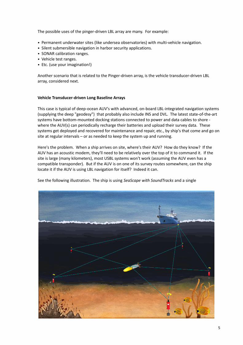
This case is typical of deep-ocean AUV's with advanced, on-board LBL-integrated navigation systems (supplying the deep "geodesy") that probably also include INS and DVL. The latest state-of-the-art systems have bottom-mounted docking stations connected to power and data cables to shore - where the AUV(s) can periodically recharge their batteries and upload their survey data. These systems get deployed and recovered for maintenance and repair, etc., by ship's that come and go on site at regular intervals – or as needed to keep the system up and running.

Here's the problem. When a ship arrives on site, where's their AUV? How do they know? If the AUV has an acoustic modem, they'll need to be relatively over the top of it to command it. If the site is large (many kilometers), most USBL systems won't work (assuming the AUV even has a compatible transponder). But if the AUV is on one of its survey routes somewhere, can the ship locate it if the AUV is using LBL navigation for itself? Indeed it can.

See the following illustration. The ship is using SeaScape with SoundTracks and a single

5

hydrophone to listen to the array's response to the AUV. The ship silently fixes the AUV's position and proceeds with it's planned activities.

Advantages:

• The same system is used during testing, deployment and recovery by anyone properly equipped.• Navigation can work for emergency "Sub down, sub sunk" if the AUV is still transmitting.• The same geodetic basis is used for ship-side location of the AUV as the AUV itself uses.

These first two examples – passive navigation on pinger-driven and vehicle-driven LBL arrays both use fully-found, off-the-shelf transponders and transceivers from different manufacturers around world. The technology is mature and reliable when applied by people who understand its proper application. SeaScape With SoundTracks extends that technology in new ways that are useful.

The next case is somewhat similar, but uses only an array of hydrophones (microphones) to listen and position just about any sound source within or near the array.

Passive Hydrophone Arrays w/Sound Sources

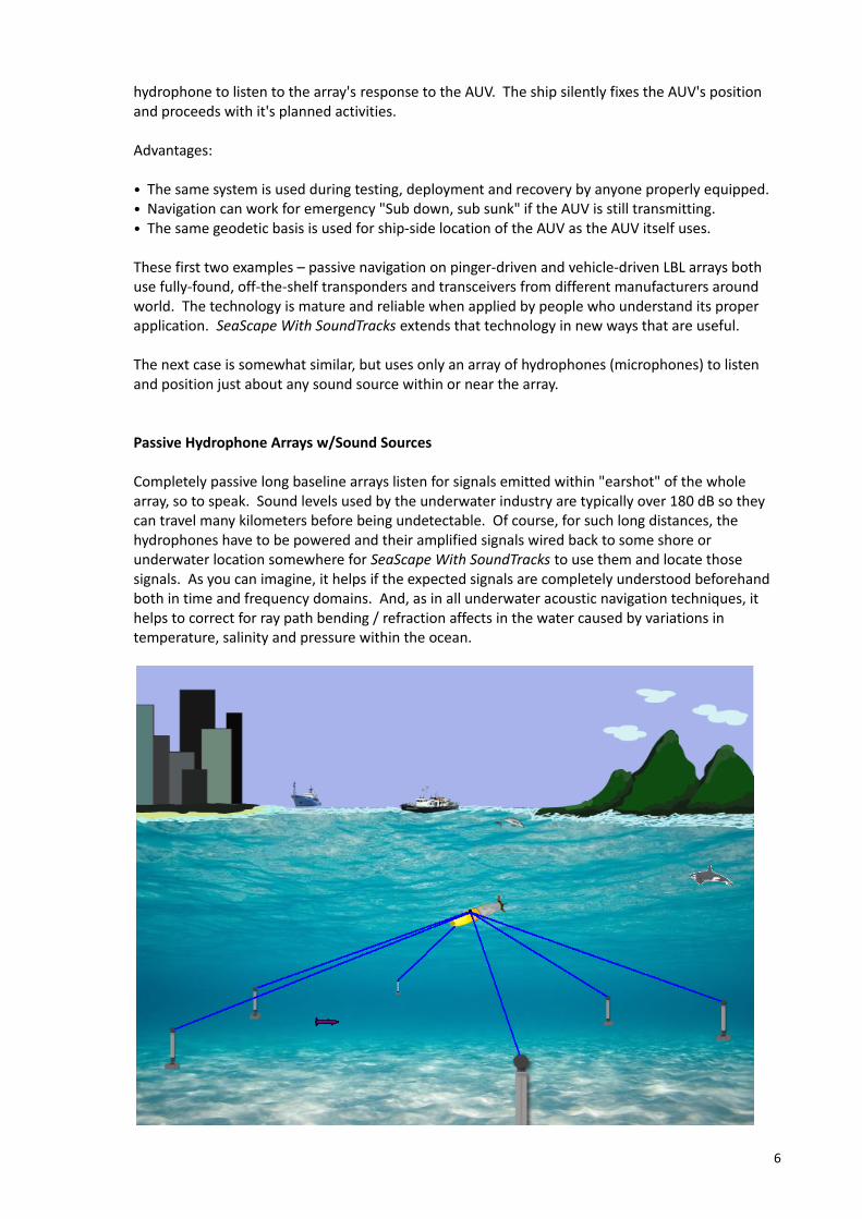
Completely passive long baseline arrays listen for signals emitted within "earshot" of the whole array, so to speak. Sound levels used by the underwater industry are typically over 180 dB so they can travel many kilometers before being undetectable. Of course, for such long distances, the hydrophones have to be powered and their amplified signals wired back to some shore or underwater location somewhere for SeaScape With SoundTracks to use them and locate those signals. As you can imagine, it helps if the expected signals are completely understood beforehand both in time and frequency domains. And, as in all underwater acoustic navigation techniques, it helps to correct for ray path bending / refraction affects in the water caused by variations in temperature, salinity and pressure within the ocean.

6

Depicted above is a hypothetical hydrophone array and an AUV with a loud pinger that transmits every so many seconds. The harbor is probably noisy. Not shown are the hydrophone's buried cables that are routed to shore where people monitor that port for intruders who shouldn't be there. The AUV has detection systems of its own and it's about to locate that red object traveling near the bottom.

The people on shore know precisely where that AUV is as it encounters and documents the intruder before surfacing (perhaps) to make its radio report, which no doubt contains information on the intruder's position for possible countermeasures.

Advantages:

• Can locate incoherent, impulse-type signals as well.• Can listen for conditions in its environment.• No active transponder array discoverable/usable by others.• Precise navigation in critical situations.

Active/Passive Wired Transponder Arrays

The best of all worlds for an "array" is a wired array with all possible modes:

• Stand alone transponder (normal LBL use)• Normal Transponder but also with differential voltage pulse to shore• Responder (strobed array transmit and passive vehicle(s) receive)• Hydrophone (listen only - passive array navigation like above)

Of course, this special type of "transponder" ("transputer?" - a different name is needed!) can't listen while it's transmitting (and for a time afterwards) similar to commercially available transponders and transceivers.

7

SeaScape With SoundTracks can navigate active acoustic objects with such wired arrays when differential voltages - OR the transponding acoustic signals themselves – OR just the passive hydrophone signals - are "brought to shore" on a pair of wires. In this first release of the system, it doesn't support "strobed transmit" of the array, however. We're hoping this will happen in the future and that, perhaps, SeaScape With SoundTracks will motivate the design and manufacture of such wired, all-modes devices!

Other Possibilities

There are more possibilities that would be a natural for SeaScape With SoundTracks but are not yet implemented.

• Vessel-mounted Short Baseline Arrays (SBL)

• Underwater structure-mounted "Small Arrays"

• Towed Arrays

We'll leave those for future discussion, perhaps.

8

The Hardware:

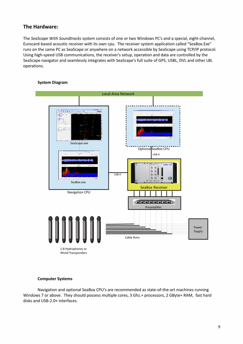
The SeaScape With Soundtracks system consists of one or two Windows PC's and a special, eight-channel, Eurocard-based acoustic receiver with its own cpu. The receiver system application called "SeaBox.Exe" runs on the same PC as SeaScape or anywhere on a network accessible by SeaScape using TCP/IP protocol. Using high-speed USB communications, the receiver's setup, operation and data are controlled by the SeaScape navigator and seamlessly integrates with SeaScape's full suite of GPS, USBL, DVL and other LBL operations.

System Diagram

Computer Systems

Navigation and optional SeaBox CPU's are recommended as state-of-the-art machines running Windows 7 or above. They should possess multiple cores, 3 Ghz.+ processors, 2 GByte+ RAM, fast hard disks and USB-2.0+ interfaces.

9

Local Area Network

SeaBox.exe

SeaScape.exe SeaBox.exe

Navigation CPU

Optional SeaBox CPU

USB-II

USB-II

Preamplifier

PowerSupply

Cable Runs

1-8 Hydrophones or Wired Transponders

SeaBox Receiver

SeaBox Receiver

The SeaBox-1000 (SB-1000) receiver is an eight-channel, high-performance, low-noise, intelligent system with it's own cpu, high-speed memory, A/D and Digital I/O hardware and extensive on-board DSP capability. The SeaBox application (SeaBox.Exe) communicates directly with the receiver using USB 2.0 communications. Further, configuration setups for SeaBox are generated by SeaScape, passed to SeaBox.Exe and downloaded to the SB-1000. The separation of SeaScape and SeaBox applications allows for SeaBox to run remotely over a network if desired for more convenient physical location.

Summary:

• 2.0 GHz Intel Celeron embedded processor• 1 Gbytes of active DDR3 memory• USB 2.0 interconnection to the host• Compatible with portable laptop systems• Eight 16-bit A/D converters• Eight configurable signal sources• 20 ns TIME resolution• 7 configurable bipolar input voltage ranges, -10V to +10V max• All channels true differential (single-ended also supported)• 1 million samples per second per converter channel• 8M samples per second aggregate• 16 bits digital inputs and 16 bits digital outputs

Physical / Electrical:

• Enclosure: 9.25" wide x 5.5" high x 12.5" deep • Power: 120 VAC• Adaptive fan cooled

Options:

• 19" rack mount version• Front Panel BNC connectors (8)• Cable options (68-pin D-Sub versus BNC)

10

Hydrophones

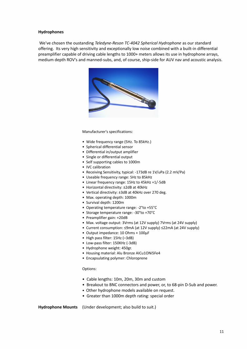
We've chosen the oustanding Teledyne-Reson TC-4042 Spherical Hydrophone as our standard offering. Its very high sensitivity and exceptionally low noise combined with a built-in differential preamplifier capable of driving cable lengths to 1000+ meters allows its use in hydrophone arrays, medium depth ROV's and manned-subs, and, of course, ship-side for AUV nav and acoustic analysis.

Manufacturer's specifications:

• Wide frequency range (5Hz. To 85kHz.)• Spherical differential sensor• Differential in/output amplifier• Single or differential output• Self supporting cables to 1000m• IVC calibration• Receiving Sensitivity, typical: -173dB re 1V/uPa (2.2 mV/Pa)• Useable frequency range: 5Hz to 85kHz• Linear frequency range: 15Hz to 45kHz +1/-5dB• Horizontal directivity: ±2dB at 40kHz• Vertical directivity: ±3dB at 40kHz over 270 deg.• Max. operating depth: 1000m• Survival depth: 1200m• Operating temperature range: -2°to +55°C• Storage temperature range: -30°to +70°C• Preamplifier gain: +20dB• Max. voltage output: 3Vrms (at 12V supply) 7Vrms (at 24V supply)• Current consumption: ≤9mA (at 12V supply) ≤22mA (at 24V supply)• Output impedance: 10 Ohms + 100μF• High pass filter: 15Hz (–3dB)• Low-pass filter: 150KHz (-3dB)• Hydrophone weight: 450gr.• Housing material: Alu Bronze AICu1ONi5Fe4• Encapsulating polymer: Chloroprene

Options:

• Cable lengths: 10m, 20m, 30m and custom • Breakout to BNC connectors and power, or, to 68-pin D-Sub and power.• Other hydrophone models available on request.• Greater than 1000m depth rating: special order

Hydrophone Mounts (Under development; also build to suit.)

11

Other Components

Preamplifier

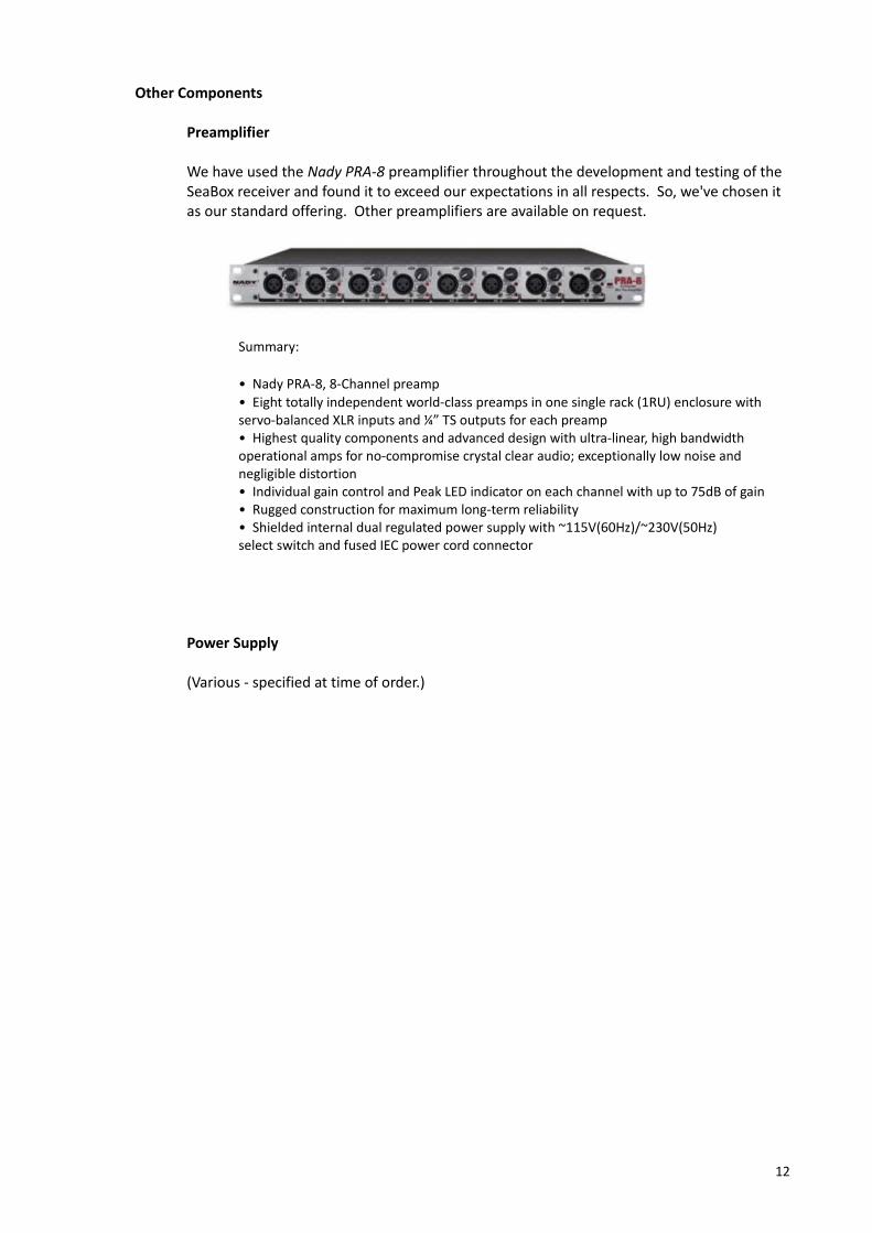
We have used the Nady PRA-8 preamplifier throughout the development and testing of the SeaBox receiver and found it to exceed our expectations in all respects. So, we've chosen it as our standard offering. Other preamplifiers are available on request.

Summary:

• Nady PRA-8, 8-Channel preamp• Eight totally independent world-class preamps in one single rack (1RU) enclosure with servo-balanced XLR inputs and ¼” TS outputs for each preamp • Highest quality components and advanced design with ultra-linear, high bandwidth operational amps for no-compromise crystal clear audio; exceptionally low noise and negligible distortion • Individual gain control and Peak LED indicator on each channel with up to 75dB of gain • Rugged construction for maximum long-term reliability • Shielded internal dual regulated power supply with ~115V(60Hz)/~230V(50Hz) select switch and fused IEC power cord connector

Power Supply

(Various - specified at time of order.)

12

The Software:

The SeaScape With Soundtracks software system consists of three parts: SeaScape.Exe, SeaBox.Exe and the SeaBox receiver's built-in program. The overall controller is SeaScape that communicates with SeaBox.Exe via direct memory transfer or by TCP/IP communications over a LAN or WAN.

SeaScape is a multi-level navigation program that has its origins decades ago in acoustic long baseline (LBL) and GPS navigation where large underwater LBL arrays are deployed, calibrated and navigated on by ROV's, manned-subs, camera tows, and so forth. As such, adding passive LBL navigation to SeaScape is a natural extension to what it already does – and in fact, is simpler to operate for the navigator than full, active LBL with all of its potential modes and complexities. Hopefully, this will become more apparent below.

The following discussion briefly illustrates the example steps necessary to produce navigation fixes typical in the various passive modes of the system, but specifically for the "Passive Ship" AUV navigation case.

SeaScape

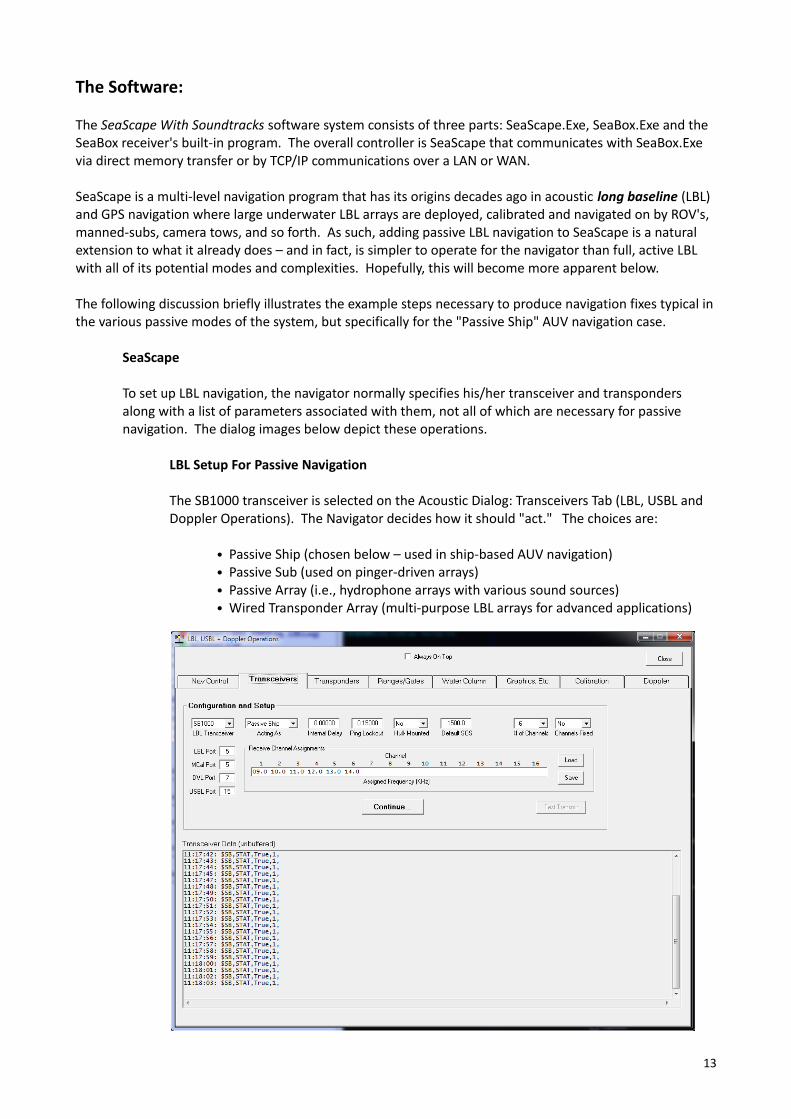
To set up LBL navigation, the navigator normally specifies his/her transceiver and transponders along with a list of parameters associated with them, not all of which are necessary for passive navigation. The dialog images below depict these operations.

LBL Setup For Passive Navigation

The SB1000 transceiver is selected on the Acoustic Dialog: Transceivers Tab (LBL, USBL and Doppler Operations). The Navigator decides how it should "act." The choices are:

• Passive Ship (chosen below – used in ship-based AUV navigation)• Passive Sub (used on pinger-driven arrays)• Passive Array (i.e., hydrophone arrays with various sound sources)• Wired Transponder Array (multi-purpose LBL arrays for advanced applications)

13

Shown above, the "Internal Delay" of the receiver is set to zero, the default Speed Of Sound (SOS) is set to 1500 m/s (as usual) and the navigator knows that five transponders and the array interrogate frequency from their AUV will be used for navigation, so he/she sets "# of Channels" to six (1-16 are possible) and then edits the "Receive Channel Assignments" frame to reflect those frequencies (here, 9.0, 10.0, 11.0, 12.0, 13.0 and 14.0 kHz).

Likewise, the pre-deployment Transponder parameters are established on the Transponders Tab shown below along with the all-important "Net Interrogate Frequency" (here, 9.0 kHz.). (Note: the transponder names shown are actually for a test setup in a small area and their UTM coordinates are near the Central Meridian of -129 degrees Longitude and the Equator!)

All of the transponder Delays ("turn around times") are set to match their manufacturer's spec's and their reply frequencies are entered along with their associated receiver channels defined previously on the Transceivers Tab (above). The post-transpond "Inhibit" (blank out) times in seconds are entered along with their "Planned" positions and depths.

There are additional settings for navigation cycle time, starting seed positions, the water column's Sound Velocity Profile, graphic symbols (etc.) but they are straight forward and not covered here. Plus, our array interrogations will come from our AUV's transducer (similar to old-fashioned "ship's 'ducer" LBL nav), so "Relay Transponder" settings are ignored.

Normally, the acoustic transponder array defined above would then be deployed and "calibrated," thus solving for the best Latitude/Longitude and Zed of each transponder. The navigator would use the Calibration Tab and Nav Control Tabs above to do that. This is a topic all in itself and beyond the scope if this brief introduction. So, consider the array above to be accurately calibrated for now.

Normally, for active LBL, the operator would return at some point (when the hardware is ready and after saving their settings) to the Transceiver Tab (above) and click the button that says "Initialize" to communicate with his/her transceiver and load key parameters for its proper operation. However, with the SB-1000 receiver, this button now says "Continue,"

14

instead, and clicking on it launches the SeaBox 1000 Configuration dialog discussed next.

SeaBox-1000 Receiver Configuration

Normally, SeaScape is configured below to "Launch SeaBox At Startup" (SeaBox.Exe). The operator could launch it now, however, and wait a few seconds for the green "Running | Reset" light before proceeding.

Next, the navigator selects the "Preset" to determine how the SeaBox Receiver program will operate. The choices are:

• Analysis• Passive Sub Receiver• Passive Ship Receiver (our case here)• Passive Array Receiver• Wired Digital Array

The "AUV nav from the ship" case under discussion is shown above. We're using one detector (hydrophone) as default "Channel 0" with a Voltage sensitivity of -167 dB and six frequencies (as defined above); we have a true differential connection and are applying a Detector Gain of 1 in the SeaBox Receiver while sampling all channels at 50,000 samples/second (which is plenty for low frequency, long baseline navigation).

We're starting out with no digital filtering selected which means all signal detection and FFT plots will be based on unfiltered data. We're polling the buffering USB hardware driver at

15

50 milisecond intervals and the Navigation Cycle Time (set on Acoustics Dialog above) is six seconds (shown in milliseconds).

In this discussion, our transponders and AUV transducer all have pulse lengths of 10 miliseconds and are treated as sine waves (even though they briefly start out as pseudo square waves) and we require a signal-to-noise ratio (SNR) of 20 to cause our hardware to trigger and attempt signal detection. Not shown above in the dropdowns are:

Signal Type: Analog or DigitalConnection Group: C0, C1, C2 (three possible slots in Receiver determining

whether D-Sub or BNC connectors are active)Detector Connection Type: Differential or Single-endedApplied Detector Gain: 1, 2, 5, 10, 20, 50, 100Digital Filtering: None; 7-17 (kHz) wide pass; 0.5 kHz band pass; 7.0 kHz high

pass, 17.0 kHz. low passPulse Type: Square wave; sine wave; differential V. pulse; user-defined

Note that had the navigator instead set up for the "Passive Array" case, he/she would have selected the frequencies for the vehicle sound sources involved ("beacons," i.e., pingers, etc) on the Acoustics Dialog above, chosen the Passive Array mode on both the Acoustic Dialog and the SeaBox 1000 Configuration dialog, and declared five or more detectors above instead of one, etc. The hydrophone positions are entered as as if they were actual transponders but the frequency assignment for them doesn't matter since the hydrophones can detect anything within their filter settings.

In any case, when done changing things on this dialog, the operator clicks the "Download Above" button and observes the commands received on SeaBox.Exe's Diagnostics Tab shown further below.

First, however, more about signal detection methods and capabilities.

Signal Template Design / Editing

The "Internal" signal ("pulse") types in SeaBox include square waves, sine waves and the differential voltages as mentioned above . For these, the assumption of an unshaped signal of full, normalized magnitude is adequate for detection of most "generic tranponders" or other sound sources. However, even more accurate and consistent signal detection is possible when the signal uses both frequency modulation and a unique "envelope." Thus the provision for "User-Defined" pulse type. SeaScape With SoundTracks provides this in two ways:

First, SeaBox.Exe allows the operator to record their signals directly, and, after proper editing in SeaScape (below), the results are a waveform file with extension ".Template" that can be passed to SeaBox during the Download process. The navigator just selects the created .Template file sources for their defined frequencies (above).

On the other hand, the desired waveform that best matches your actual device can, instead, be designed in SeaScape using the Design button on the SeaBox 1000 Configuration dialog.

16

The Template Designer result of a user-designed, MFSK-encoded ("Multiple Frequency Shift Keying") and shaped signal template is shown above. When first starting this process, the user selects the following.

Signal Type: Monotone, Up-chirp, Down-chirp, (Encoded, Sampled)Basic Waveforms: Square Wave, Sine Wave, (Variable)Pulse Length: 1 – 10 msec.

If designing a linear chirp signal, the user enters the desired beginning and ending frequencies of the chirp and finally clicks on Create. If intending to encode a basic waveform instead with a MSFK or PSK method, they first select a monotone square or sine wave signal type, click on Create, then select "Encode" as a Signal Type and then use the Encode Icon button. This results in launching the Signal Encoding dialog:

17

For MFSK encoding, after defining their unique frequencies and their cycle counts ("#Cycles") they click on Apply/Close and then the Create button on the Template Designer one last time. A typical result is shown on the first dialog image above.

PSK ("Phase Shift Keying") is performed in a similar manner except PSK encoding uses a user-supplied "Elapsed Time" and "Start Phase" number for each frequency interval desired.

For signal shaping, the provided Mouse Edit functions allow the user to zoom, shape, delete blocks of points, move points, de-noise the data, invert all values, and finally, undo their actions if they make a mistake. Loading SeaBox's .CSV recordings or existing .Template files and Saving edited signal .Template(s) are also supported - as is viewing FFT's of 2048-point buffers.

For producing signal .Template files from SeaBox's .CSV recordings, the precise number of "Points" required in the waveform is determined by your Sample Rate and Pulse Width. In the above case, the number is an easy to remember 500 points. In this particular case, when loading a .CSV file to convert to a .Template, one would delete the unwanted points with the delete block mouse tool to exactly 500 total and then save the (automatically-) normalized results to a .Template named appropriately.

Finally, note that your defined encoding methods themselves may be conveniently saved or loaded to/from file for future use.

SeaBox

SeaBox.Exe has three tabs in its user interface: Diagnostics, Analysis and Navigation. These will be discussed in order.

Diagnostics

As SeaBox.Exe starts up with the Diagnostics Tab selected, the navigator can immediately observe the results of his/her "Download" action from the SeaBox 1000 Configuration dialog (above) in the Processor Administration and SeaScape Commands text boxes, as well as in the Current Settings Frame at the bottom (see below).

Since SeaBox defaults to dynamic memory exchange between it and SeaScape, that radio button in the COMM's frame will be selected at startup. If the user desires operation over a network, the SeaScape IP address and port must be entered and then the TCP / Network radio button selected.

After initialization from SeaScape, the user may then use the Start / Stop buttons on the dialog for normal operations. Start / Stop is also available on SeaScape's SeaBox 1000 Configuration dialog (above) for remote network operation. When the navigator presses Start, whatever mode that was declared in the download (above) will start to execute with the navigation cycle time in effect, even for "Analysis" mode.

To change running modes, the user must Stop whatever mode they are running and use the Configuration dialog above to make major changes, download the new settings again and press Start again as before. This usually takes only seconds to do.

18

Whereas most of the data from the SeaBox Receiver is in binary format, the data posted in the Processor Data box is converted to ASCII for easier reading.

Buffers and communication pipes usage may also be examined using the Buffers + Pipes Stats button.

Analysis

When arriving on site, the navigator will often start out by analyzing the acoustic conditions around their ship or vehicle to determine general noise levels and anomalies that might interfere with consistent acoustic navigation. Interferring 12 kHz. fathometers, acoustic Doppler current profilers, swath sonars, etc., left on by mistake at the start of critical acoustic navigation will be apparent. Acoustic sound sources aready in the water column can also be monitored and their signal strengths and frequency spectrums observed over time. We think the ability to analyze one's acoustic environment before and during navigation is vital.

The Analysis Tab can be observed in all running modes of SeaBox.Exe. However, only in the "Analysis Mode" itself is the live Signal Plot (top) active for the detector channel selected (0-7). The FFT plot at the bottom of the tab remains active in all navigation modes, however.

19

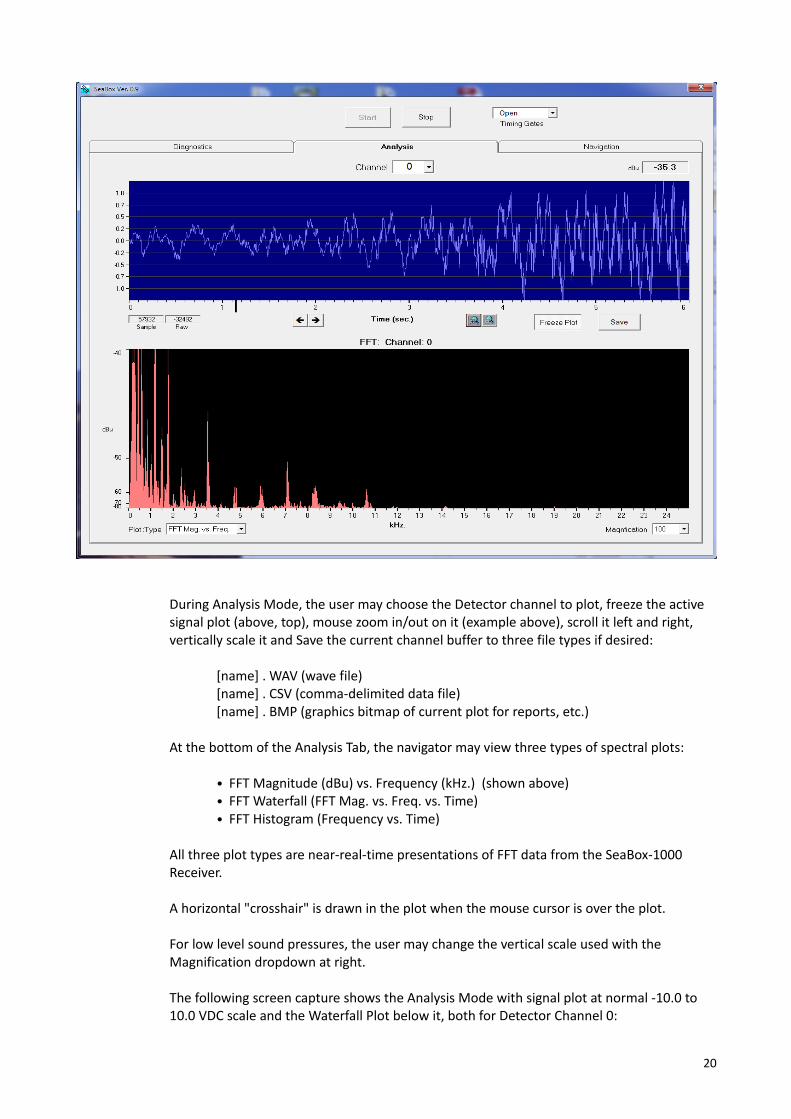
During Analysis Mode, the user may choose the Detector channel to plot, freeze the active signal plot (above, top), mouse zoom in/out on it (example above), scroll it left and right, vertically scale it and Save the current channel buffer to three file types if desired:

[name] . WAV (wave file)[name] . CSV (comma-delimited data file)[name] . BMP (graphics bitmap of current plot for reports, etc.)

At the bottom of the Analysis Tab, the navigator may view three types of spectral plots:

• FFT Magnitude (dBu) vs. Frequency (kHz.) (shown above)• FFT Waterfall (FFT Mag. vs. Freq. vs. Time)• FFT Histogram (Frequency vs. Time)

All three plot types are near-real-time presentations of FFT data from the SeaBox-1000 Receiver.

A horizontal "crosshair" is drawn in the plot when the mouse cursor is over the plot.

For low level sound pressures, the user may change the vertical scale used with the Magnification dropdown at right.

The following screen capture shows the Analysis Mode with signal plot at normal -10.0 to 10.0 VDC scale and the Waterfall Plot below it, both for Detector Channel 0:

20

The Waterfall Plot refreshes and draws continuously for every Navigation Cycle showing you the spectral components in the signal during the Navigation Cycle. This type of plot is often used to show the nature of the sound in the water (its frequencies and sound levels), often referred to "broadband noise." Of course, it will also show you whatever signal sources are present. Comparing sound levels between different ships and at different ocean sites can be very important to reduce the unknowns of underwater acoustic navigation.

The filter settings in use will affect what's observed on the Waterfall (and other plots) and the operator may select different filters (above) and observe their effect.

The Histogram plot is shown next as yet another common way of displaying spectral data over time. Once again, the operator may adjust his/her "magnification" for very quiet or noisy situations to better view the dominant frequencies being received by SeaBox.

(There is no deliberate "Save" of the FFT plots in the current release. If you need to save them, you can always use the Windows "Alt-Print Scrn" bitmap capture keys and paste the Windows clipboard into a graphics program that supports clipboard pasting.)

21

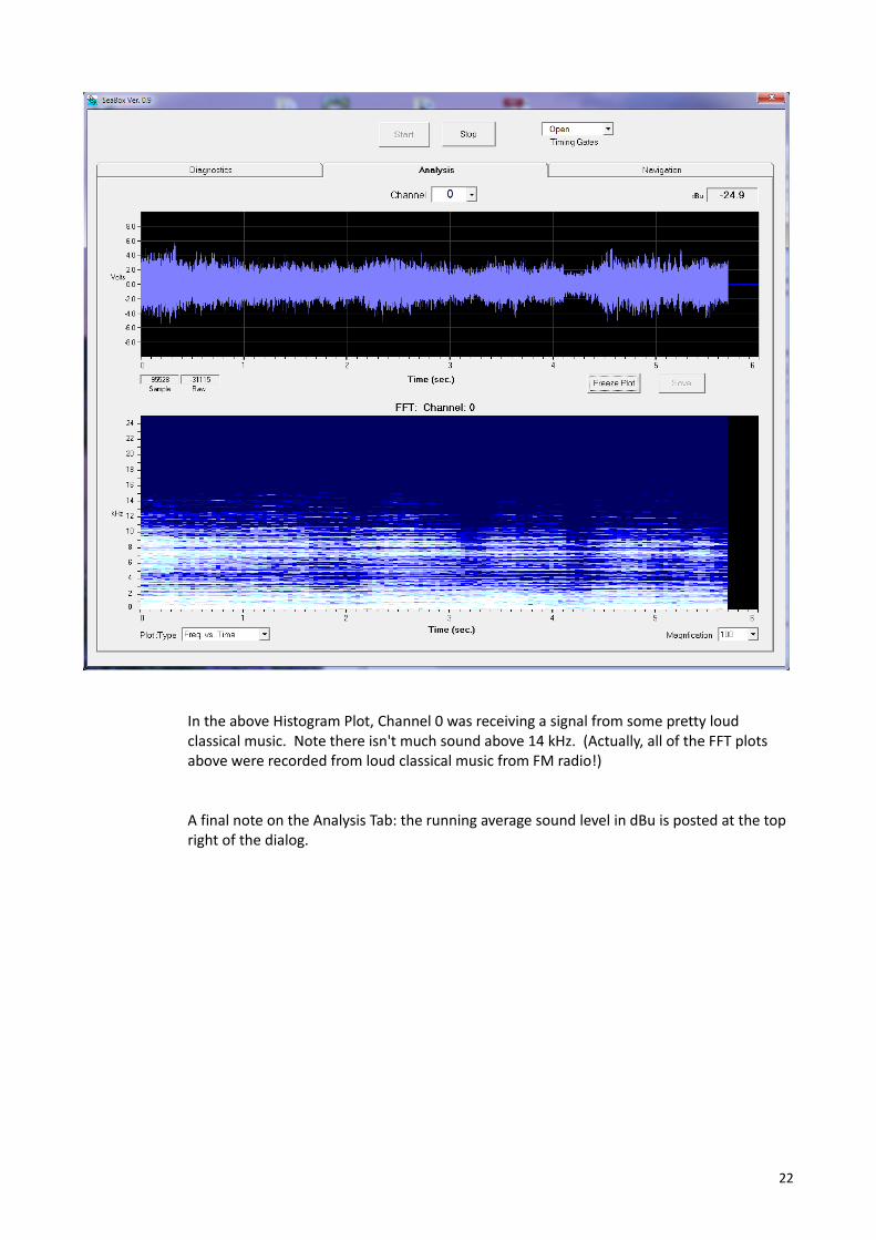
In the above Histogram Plot, Channel 0 was receiving a signal from some pretty loud classical music. Note there isn't much sound above 14 kHz. (Actually, all of the FFT plots above were recorded from loud classical music from FM radio!)

A final note on the Analysis Tab: the running average sound level in dBu is posted at the top right of the dialog.

22

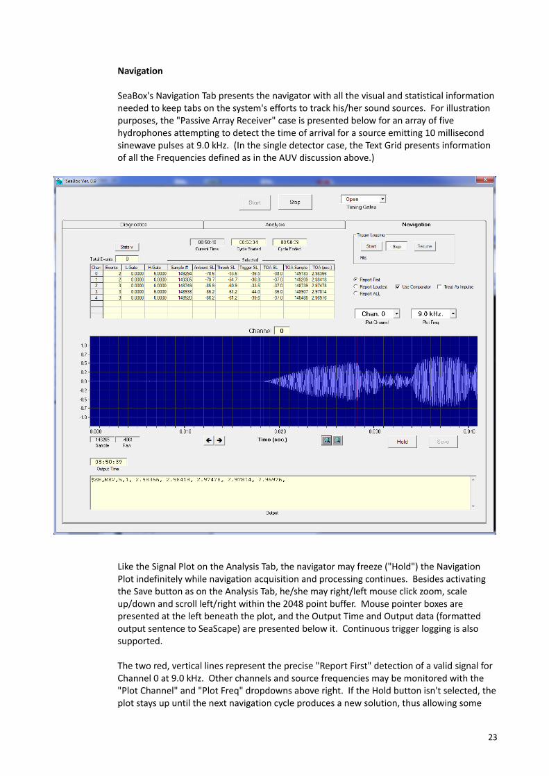
Navigation

SeaBox's Navigation Tab presents the navigator with all the visual and statistical information needed to keep tabs on the system's efforts to track his/her sound sources. For illustration purposes, the "Passive Array Receiver" case is presented below for an array of five hydrophones attempting to detect the time of arrival for a source emitting 10 millisecond sinewave pulses at 9.0 kHz. (In the single detector case, the Text Grid presents information of all the Frequencies defined as in the AUV discussion above.)

Like the Signal Plot on the Analysis Tab, the navigator may freeze ("Hold") the Navigation Plot indefinitely while navigation acquisition and processing continues. Besides activating the Save button as on the Analysis Tab, he/she may right/left mouse click zoom, scale up/down and scroll left/right within the 2048 point buffer. Mouse pointer boxes are presented at the left beneath the plot, and the Output Time and Output data (formatted output sentence to SeaScape) are presented below it. Continuous trigger logging is also supported.

The two red, vertical lines represent the precise "Report First" detection of a valid signal for Channel 0 at 9.0 kHz. Other channels and source frequencies may be monitored with the "Plot Channel" and "Plot Freq" dropdowns above right. If the Hold button isn't selected, the plot stays up until the next navigation cycle produces a new solution, thus allowing some

23

time to inspect the plots for other channels or frequencies without holding the plot.

Above the plot is a text grid displaying the stat's for the particular navigation cycle that produced the Output Data to SeaScape for its fix computations. Ambient, Threshold, Trigger and Time Of Arrival sound levels ("SL") are presented along with the sample number and its corresponding Time of Arrival in seconds since the cycle began. The number of trigger events per channel along with the low and high timing gate settings are also presented. A Total Events count for the cycle is shown above the grid. The Total Events box clears at the start of a new Navigation Cycle.

Navigation in SeaScape

Since any passive system can only detect signals and not originate them, some kind of coordination is needed to synchronize with regularly-timed sound sources in the water. In the single hydrophone case, the timed source is the transducer on the vehicle or the pinger on the bottom that transmits every N seconds, thus interrogating the bottom array. In this case, SeaScape detects the arrival time of this "Net Interrogate" signal (which should arrive first) and adjusts the SeaBox timing appropriately to always keep the tranponder replies arriving within the SeaScape/SeaBox "Navigation Cycle" (and not overlapping the cycle, as is possible).

For the Passive Hydrophone Array case, SeaScape informs SeaBox when it has a good fix based on input arrival times. SeaBox then adjusts it's cycle start timing to keep the entire group of anticipated, future detections within the Navigation Cycle.

Of course, it's very important that the navigation "Cycle Time" in SeaScape (as downloaded to SeaBox) be the same as any bottom or vehicle ping interval. And for multiple vehicles operating on a hydrophone array, it's clear that their ping intervals should be identical but best offset somewhat in their start times in case the vehicles are in close proximity.

For single hydrophone navigation (Passive Sub and Passive Ship), SeaScape uses the "Mooring Transducer" as the hydrophone position and the "LBL Transducer" fix object for the fix generated (normally associated with the vessel in active LBL navigation).

For navigation with hydrophone or wired transponder arrays, SeaScape assigns fixes to "Relay Transponder" fix objects starting with "LBL Relay #1" for as many frequencies defined.

Thus, assigning to existing SeaScape fix objects allows the navigator to treat any passive fixes as they would for active LBL, USBL or DVL navigation with all of the normal features of SeaScape available to them (Grid symbols, object-to-object relationships, logging, custom output, integration with vehicle sensors, filtering, and so forth).

Shown below is an actual test setup producing actual fixes in a lab using a very small, five-channel microphone array. Fixes of the small, green ROV shown are good to about 2 centimeters.

24

Using SeaScape's extensive pass-through and custom output features, SeaScape with SoundTracks can be part of a larger system where navigation data is routed to other mission-critical systems. Data is faithfully logged in SeaScape and available for replay.

Calibration of Hydrophone Arrays

Passive arrays of hydrophones (or wired transponders) normally need to be 'calibrated' after deployment, i.e., their positions determined as accurately as possible prior to use. Two platforms running SeaScape are used to perform this task, one on a vessel, and one on shore connected to all the hardware. An RF modem or Ethernet bridge is used to link the two systems together for acquisition of calibration data in both locations. The vessel uses a very accurate GPS, gyrocompass and vessel dimensions and offsets along with a known sound source such as an acoustic deck set with transducer to transmit signals to the hydrophones. The vessel transmits it's station coordinates to shore at the time of transmit and the shoreside SeaScape With Soundtracks records all signal arrivals along with the vesel station. That data is then processed to produce calibrated hydrophone positions in the shoreside SeaScape.

The vessel need not know where the hydrophones were actually deployed to perform its part in the calibration. In addition, the vessel position and calibration route can be observed and managed from the shoreside stations as desired.

25

Theory:

Range-Range Positioning

The traditional, spherical, least-squares method for positioning an acoustic object uses three or more corrected range legs (four for full 3-D fixing) and a system of equations that solves for the changes in position such that the error function is minimized:

E = Σ Fi [Ri - Di]²

where:

i = 1 to N = the number of transpondersFi are the valid flags for each transponder (1=good, 0=absent)Ri are the resulting, iterated slant ranges to each transponderDi are the acoustically measured range legs to each transponder

In order to carry out this solution, the error function is differentiated with respect to the variables u, v, and w, example:

δE/δu = Σ Fi (Ri - Di) (u - xi) / Ri = Σ Fi ∆Ri cos(αi)

where x, y, and z, are coordinates of the transponders and u, v, w is the presumed position or "seed" (similarly for δE/δy and δE/δz), and the results summed to form a system of equations based on the gradient of the error function:

G [δE/δu, δE/δu, δE/δu] = [ A ] [∆u ∆v ∆w ] = [δE/δu, δE/δu, δE/δu]

where ∆u, ∆v, ∆w is the solution vector and represents the change in x, y, z of the solution. The process is repeated until a specified precision is reached, i.e., ∆E is less than some value. The solution is economically executed via Cramer's rule which works fine for 3 x 3 matrices on the computer (one of the few cases where that's true). Care must be taken to take the opposite of the gradient vector for the solution to converge.

One convenient way of picturing how this method works is to imagine a quasi-bowl-shaped 4-D surface produced by the error function with an absolute minimum at some x,y,z which nearly - but not quite - matches the true position (since all measurements have error). If you start some distance away from the truth you will find yourself up on the mountain where the error between your measurements and your presumed position is large. You then travel downhill (opposite the gradient vector) to finally reach a point where your error is satisfactorily small. The error at that point is generally computed as either the standard deviation or root mean square (RMS) of the difference between the range legs of your final, computed position and your measured range legs. (We normally use "RMS.") Assuming that your transponder positions are indeed accurate, the smaller the error, the higher your confidence in the fix.

This traditional approach assumes, of course, that you and your array remain fixed during range measurements and that actual range measurements are made and not something else, like range differences or Doppler shifts, etc. If not, you will have significant errors or need another method. The traditional method is therefore static and, although powerful, is of limited usefulness. An illustration is provided below to help visualize it.

26

Hyperbolic Range-difference Positioning: HYPERINGSTM

If measured "ranges" (geometric length based on the usual notion of "rate x time") are not available but just "arrival times" are, there is a method that produces range differences that can be used to derive a solution. We call our method "HYPERINGS."

27

For any object's assumed position based on its coordinates u,v,w, there is a matrix of the differences in the range legs to the receiving array whose coordinates are defined by xi, yi, zi, and xj, yj, zj:

rdiff ij = [ (u - xi)² + (v - yi)² + (w - zi)² ]1/2 - [ (u - xj)² + (v - yj)² + (w - zj)² ] 1/2

As you can imagine, the diagonal of this matrix is all zeroes and the lower triangular half is the opposite of the upper. This matrix presumes straight lines connecting the object with the array points. Your navigation system just receives the arrival times at each array point and we compute a similar matrix to rdiff but based on actual measurements. Calling this matrix DelR ij we can construct an all-important error function:

E = Σ Σ [ rdiff ij - DelR ij ]²

This function assumes, for the time being, that all detectors received a signal and the double summation simply reflects the relevance of only the upper triangular part of each matrix. What we're using here is the squared difference of the theoretical range leg differences and the measured range leg differences. In effect, we're looking at a "difference of differences," an important insight. As usual, we want a system of equations that solves for the three unknowns so we use a similar technique:

δE/δu = Σ Σ ( rdiff ij - DeIR ij ) [ ( (u – xi) / Ri ) - ( (u – xj) /Rj ) ]

and so forth for the other two partial derivatives. The result is, that, from some reasonable starting seed assumption combined with our measurements of arrival times and computation of measured range differences, we are able to determine the x, y, z of some remote transmitting object. And of course, the object's transmitting behavior needs to correspond with the capabilities of our receiver. The beauty of this method is that it leaves open the entire question of how a signal is recognized and validated for range difference computation. All you need to do is hand HYPERINGS an accurate set of arrival times from a geometrically-known array and it will tell you where that signal came from.

Sound Pressure Levels

Absolute sound pressure level in underwater acoustics is normally defined in decibels (dB) as:

dB = 20 log10 ( p / p0 )

where p0 is the reference value of 1 μPa (one microPascal = 10-6 kg / m s2 = 10-6 Newtons / m2)

Since "full scale" is determined by variable amplification and gain settings, SeaBox computes sound pressure levels in "dBu" which is the scale associated with non-absolute pressure that depends on any measurement's relative value to the system's "full scale measurement." This is typical of modern audio systems whose highest input (or output) is "0 dBu." All other possible values are negative.

dBu = 20 log10 ( X / [full scale reference] )

where [full scale reference] = +32767. At X = +32767, dBu = 0.

Using the full 16-bits of data to represent audio, SeaBox has approximately 96 dB of "dynamic range."

28