introduction to space syntax analysis software -...

Bauhaus-Universität Weimar 1 Decoding Spaces

Depthmap Introduction to Space Syntax Analysis Software

Dipl.-Ing. Sven Schneider


Download Depthmap

https://github.com/downloads/SpaceGroupUCL/Depthmap/DepthmapSetup1014.exe

https://github.com/downloads/SpaceGroupUCL/Depthmap/DepthmapSetup1014.exe


What is Depthmap?

“It is a tool for topological analysis The analysis of layouts is achieved through the juxtaposition of graphs The graphs are analysed“ Possible Types of Analysis are: • Convex Space Analysis

• Axial Line Analysis

• Segment Analysis

• Visibility Graph Analysis (including single

Isovists & Isovist Fields)

• Agent Analysis


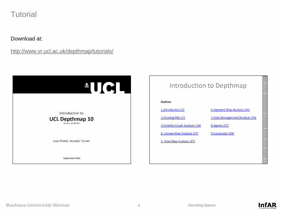
Tutorial

Download at: http://www.vr.ucl.ac.uk/depthmap/tutorials/

http://www.vr.ucl.ac.uk/depthmap/tutorials/


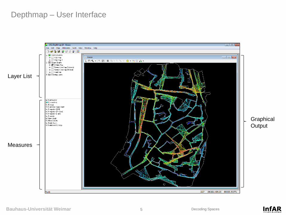
Depthmap – User Interface

Layer List

Measures

Graphical

Output


Importing Plans

Depthmap is a pure Analysis Tool, it is not possible to draw plans! Depthmap can import 2-dimensional Plans. Fileformat working best is DXF (AutoCAD 2000 Standard) After creating a new file (File New), you can import a plan (Map Import…) After importing, the plan is visible in the „Drawing Layers“ list. It is possible to import a number of plans. For each a new folder is added to the „Drawing Layers“ list. If your DXF File has different layers, these layers will be obtained in Depthmap. (This can be useful for analysing different design variants)


Representations of space: Axial Lines, Convex Spaces und Isovists


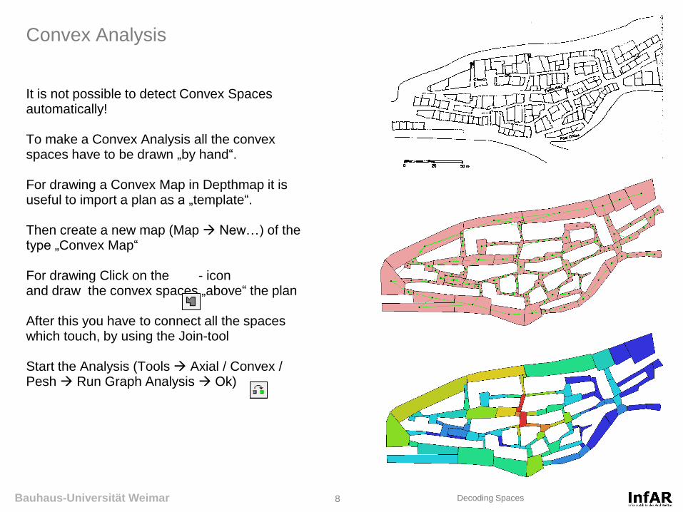
Convex Analysis

It is not possible to detect Convex Spaces automatically! To make a Convex Analysis all the convex spaces have to be drawn „by hand“. For drawing a Convex Map in Depthmap it is useful to import a plan as a „template“. Then create a new map (Map New…) of the type „Convex Map“ For drawing Click on the - icon and draw the convex spaces „above“ the plan After this you have to connect all the spaces which touch, by using the Join-tool Start the Analysis (Tools Axial / Convex / Pesh Run Graph Analysis Ok)


Exercise: Convex Map

Create new file Import the plan „InfAR_office.dxf“ Create new Map (Map Type: Convex Map) Draw Convex Spaces Connect Convex Spaces Run Graph Analysis (Tools Axial / Convex / Pesh) Check Measures (Integration, Connectivity)


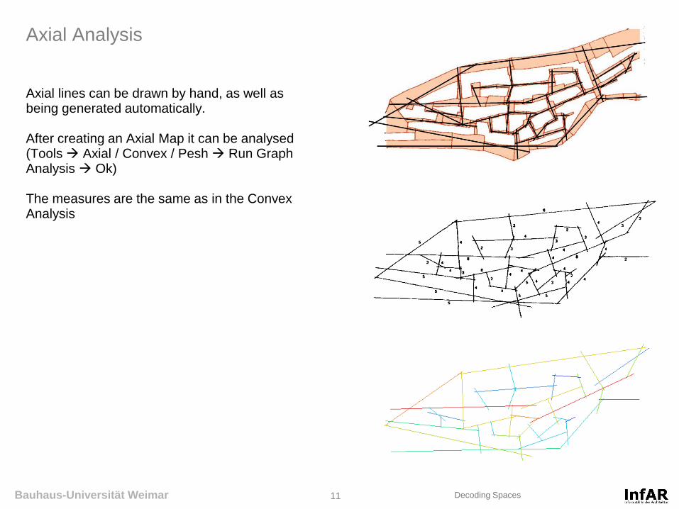
Axial Analysis

Axial lines can be drawn by hand, as well as being generated automatically. After creating an Axial Map it can be analysed (Tools Axial / Convex / Pesh Run Graph Analysis Ok) The measures are the same as in the Convex Analysis


Drawing Axial Maps

Axial Maps can be drawn by hand, as well as generated automatically. To draw an Axial Map first a new map must be created (Map New… Axial Map) After clicking on the drawing icon Axial Lines can be drawn. Before drawing the Axial Map it is useful to import a plan as a „template“. Note: You can also import a „hand-drawn“ Map as an Axial Map. This way you can use your favourite CAD-Tool.


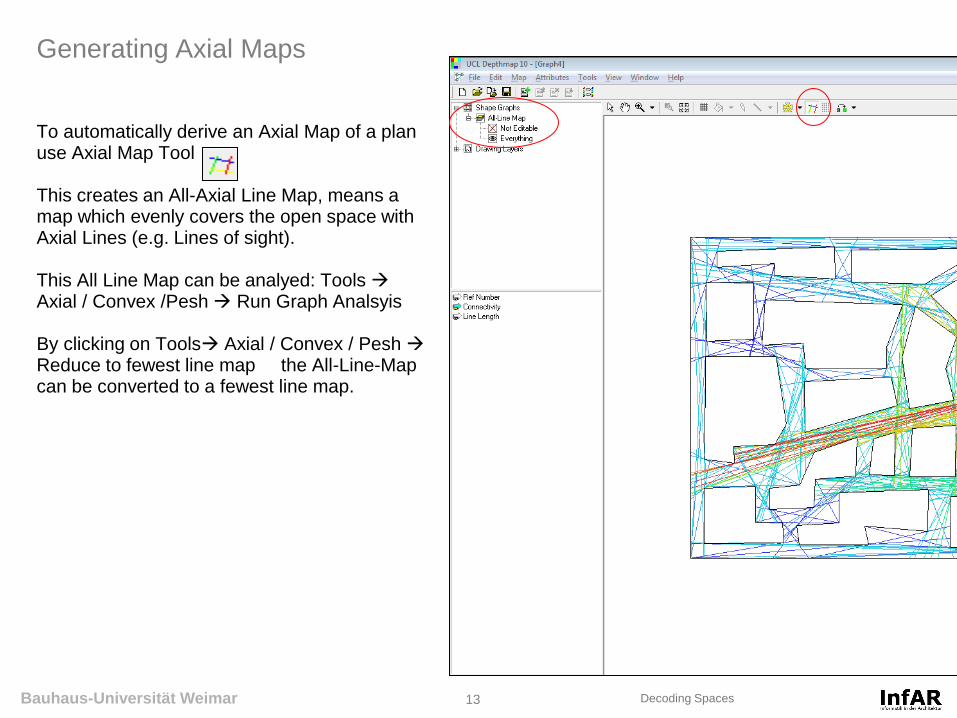
Generating Axial Maps

To automatically derive an Axial Map of a plan use Axial Map Tool This creates an All-Axial Line Map, means a map which evenly covers the open space with Axial Lines (e.g. Lines of sight). This All Line Map can be analyed: Tools Axial / Convex /Pesh Run Graph Analsyis By clicking on Tools Axial / Convex / Pesh Reduce to fewest line map the All-Line-Map can be converted to a fewest line map.


Algorithm for Generating All Line Maps

Taken from: Turner, Penn & Hillier (2005)


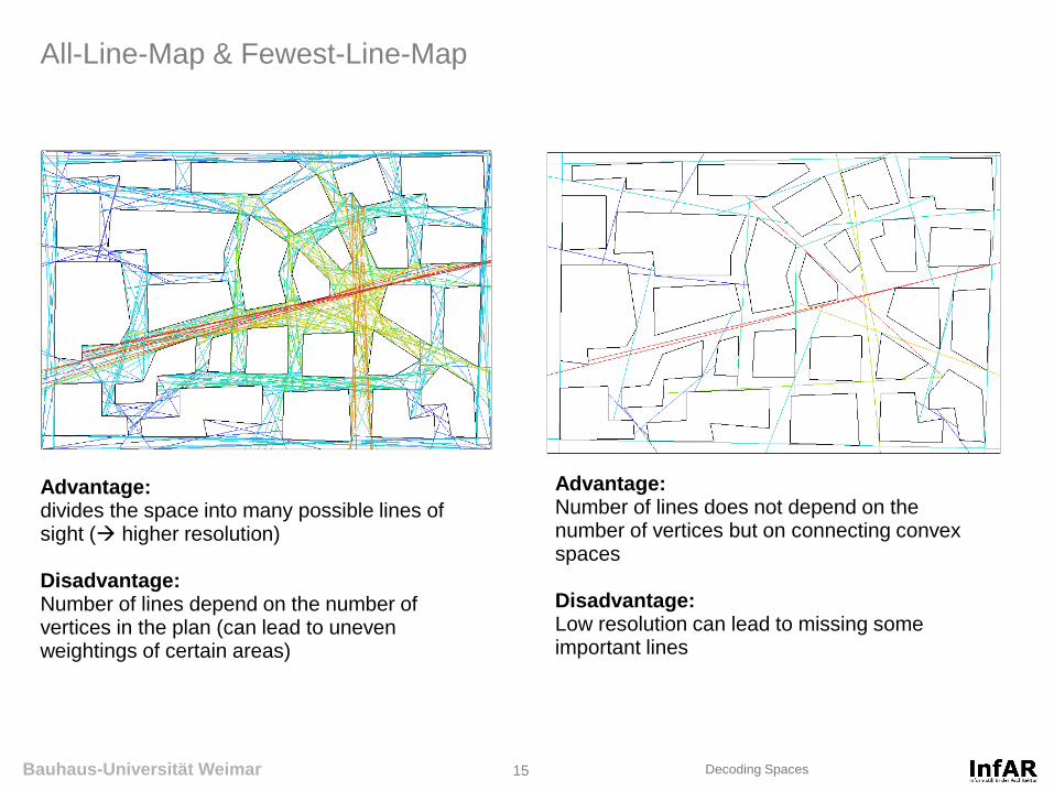
All-Line-Map & Fewest-Line-Map

Advantage: divides the space into many possible lines of sight ( higher resolution) Disadvantage: Number of lines depend on the number of vertices in the plan (can lead to uneven weightings of certain areas)

Advantage: Number of lines does not depend on the number of vertices but on connecting convex spaces Disadvantage: Low resolution can lead to missing some important lines


Overview: Graph Measures (Axial Maps, Convex Maps)

Connectivity Number of elements, which are connected to a certain element Integration Distance of an element to (all) other elements in relation to the number of elements in the complete system (To-Movement, Centrality) Choice Indicates how often a element is passed, when calculating the shortest paths between elements (Through-Movement) Control / Controllability Entropy / Relativised Entropy Intensity


Connectivity

Connectivity measures the number of elements, which are connected to a certain element. Connectivity is a local measure, means it only takes into account the direct neighbours of an element. Connectivity = 3

Connectivity in an All-Line-Map


Integration (To-Movement, Closeness)

Integration misst wie weit entfernt sich ein Element (bspw. Axial Line) in Relation zu (allen) anderen Elementen befindet. Integration is a global measure, means it only takes into account the relations of all element to an element. Der Wert wird in der Graphenanalyse auch als Zentralität bezeichnet. RRA, RA, Total Depth, Mean Depth sind Werte, die sich nur durch Umrechnung (Normalisierung, etc.) von Integration unterscheiden.

Depth = 13

Integration in an All-Line-Map


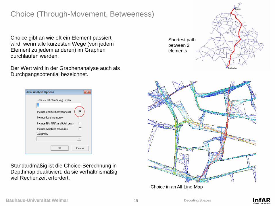
Choice (Through-Movement, Betweeness)

Choice gibt an wie oft ein Element passiert wird, wenn alle kürzesten Wege (von jedem Element zu jedem anderen) im Graphen durchlaufen werden. Der Wert wird in der Graphenanalyse auch als Durchgangspotential bezeichnet. Standardmäßig ist die Choice-Berechnung in Depthmap deaktiviert, da sie verhältnismäßig viel Rechenzeit erfordert.

Choice in an All-Line-Map

Shortest path

between 2

elements


To-Movement & Through-Movement (Integration & Choice)

Look at: http://www.slideboom.com/presentations/292558/Intro-to-Space-Syntax_Day-1

http://www.slideboom.com/presentations/292558/Intro-to-Space-Syntax_Day-1











Exercise: Axial Analysis

Create new file Import „Grasse.dxf“ Create All-Line Map Run Graph Analysis (Tools Axial / Convex / Pesh) Check Measures (Connectivity, Integration, Choice) Reduce to fewest line map and analyse it. Compare the results with the All Line Map


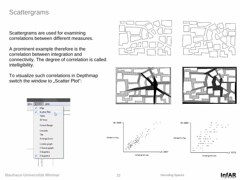
Scattergrams

Scattergrams are used for examining correlations between different measures. A prominent example therefore is the correlation between integration and connectivity. The degree of correlation is called intelligibility. To visualize such correlations in Depthmap switch the window to „Scatter Plot“:


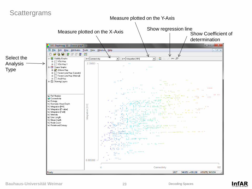
Scattergrams

Measure plotted on the X-Axis

Measure plotted on the Y-Axis

Select the

Analysis

Type

Show regression line Show Coefficient of

determination


Global and local analysis

Global analysis takes into account the relations of all elements to all elements. Local analysis takes into account relations in a certain distance / radius of each element

Global Integration Local Integration


Global and local integration

The radius defines to which depth from the original element other elements are taken into account for calculating its depth in the system. “Radius-3 integration presents a localised picture of integration, and we can therefore think of it also as local integration, while radius-n integration presents a picture of integration at the largest scale, and we can therefore call it global integration.” (Hillier, 1996) Note: Integration R1 = Connectivity

Depth, R2 = 1+1+2+2 = 6

Depth, R3 = 1+1+2+2+3+3 = 12

Depth, Rn = 1+1+2+2+3+3+4+4 = 20

1

2

3

4


Segment Analysis

In this type of Analysis not the longest lines of sight are taken into account, but the segments between intersecting lines. For calculating the graph measures not the steps from one to another element are counted, but the angles between the intersecting points of the elements. Advantages of Segment Analysis: - more detailed - better correlation with movement analysis

(Hillier & Iida, 2005)

Segment Map

Axial Map

Look at: http://www.slideboom.com/presentations/293659/Intro-to-Space-Syntax_Day-2











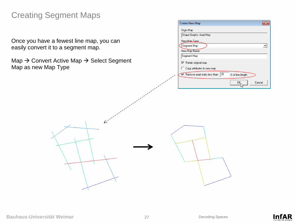
Creating Segment Maps

Once you have a fewest line map, you can easily convert it to a segment map. Map Convert Active Map Select Segment Map as new Map Type


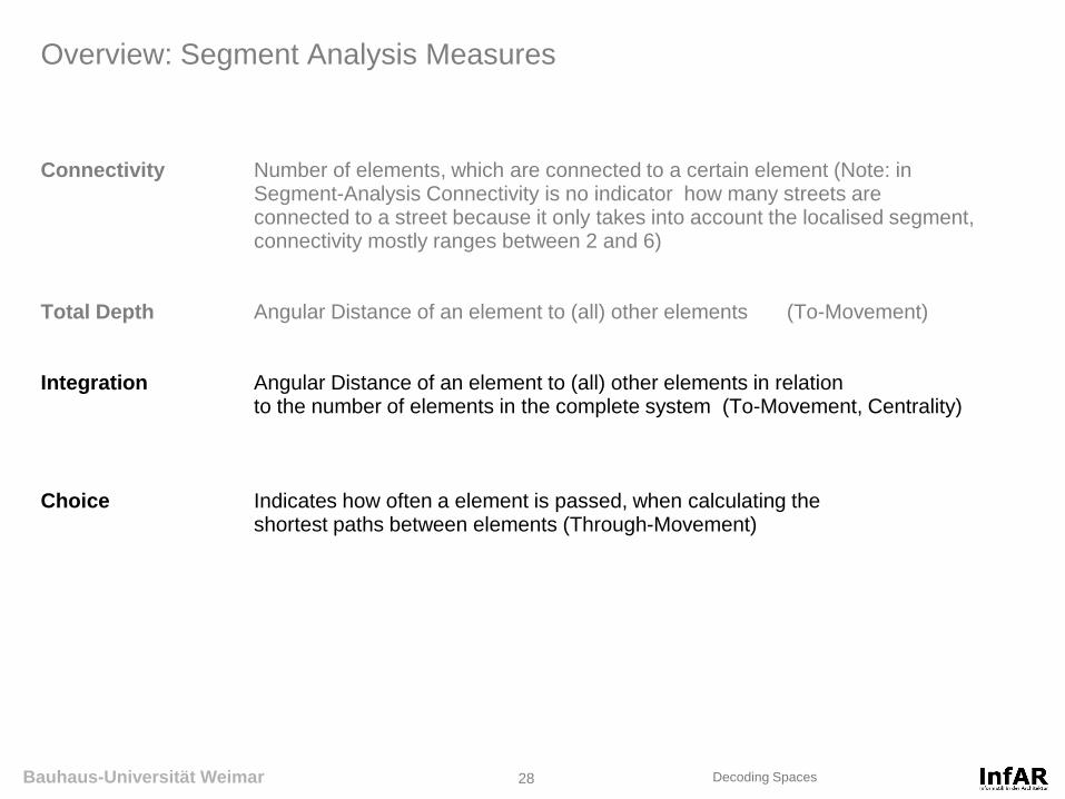
Overview: Segment Analysis Measures

Connectivity Number of elements, which are connected to a certain element (Note: in Segment-Analysis Connectivity is no indicator how many streets are connected to a street because it only takes into account the localised segment, connectivity mostly ranges between 2 and 6) Total Depth Angular Distance of an element to (all) other elements (To-Movement) Integration Angular Distance of an element to (all) other elements in relation to the number of elements in the complete system (To-Movement, Centrality) Choice Indicates how often a element is passed, when calculating the shortest paths between elements (Through-Movement)


Total Depth (Segment Analysis)

Total Depth in Segment Analysis does not take into account the steps from one segment to another, but angles between segment-intersections. 0° means a step-depth of 0.0 . . . 45° means a step-depth of 0.5 . . . 90° means a step-depth of 1.0 . . .

td = 1.07 + 0.07 + 0.05 +

1.1 + 0.06 + 0.1 + 0.47 +

0.1 = 2,85


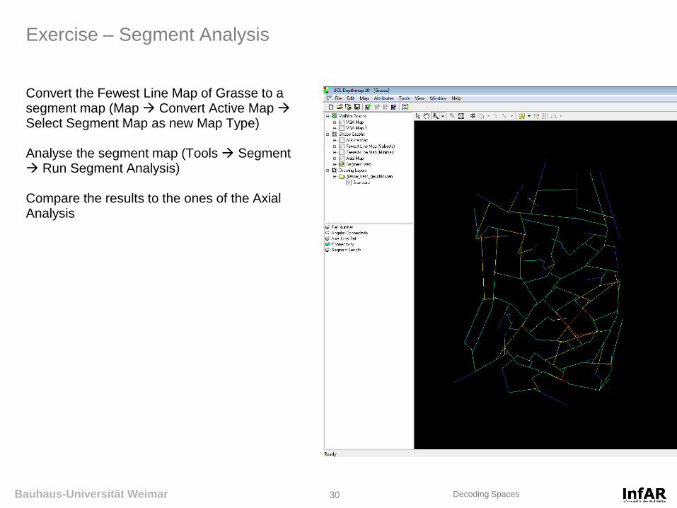
Exercise – Segment Analysis

Convert the Fewest Line Map of Grasse to a segment map (Map Convert Active Map Select Segment Map as new Map Type) Analyse the segment map (Tools Segment Run Segment Analysis) Compare the results to the ones of the Axial Analysis


Isovists

By Clicking on the Isovist Icon you can create Isovists. You can create multiple Isovists and compare their properties by clicking on the different Isovist Measures in the Measures-List. For deleting Isovists, you have to switch on the „Editibale“-Mode in the Layer-List. (Note that sometimes Depthmap is buggy and does not delete Items properly!)


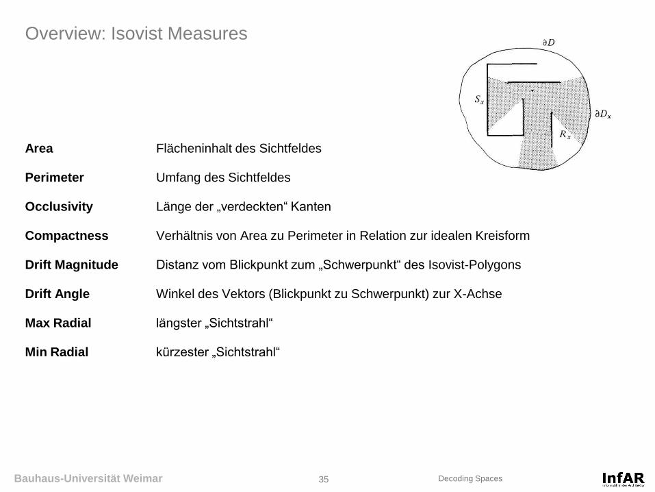
Overview: Isovist Measures

Area Flächeninhalt des Sichtfeldes Perimeter Umfang des Sichtfeldes Occlusivity Länge der „verdeckten“ Kanten Compactness Verhältnis von Area zu Perimeter in Relation zur idealen Kreisform Drift Magnitude Distanz vom Blickpunkt zum „Schwerpunkt“ des Isovist-Polygons Drift Angle Winkel des Vektors (Blickpunkt zu Schwerpunkt) zur X-Achse Max Radial längster „Sichtstrahl“ Min Radial kürzester „Sichtstrahl“


Isovist Measures - Examples

Area:

Perimeter:

Occlusivity:

Compactness:

400

70.8

0.0

1.0

400

80

0.0

0.78

298.1

486.6

416.5

0.015

circle square forest


Isovist Field

“to quantify a whole configuration, more than a single isovist is required and he suggests that the way in which we experience a space, and how we use it, is related to the interplay of isovists” “Isovist fields record a single isovist property for all locations in a configuration”


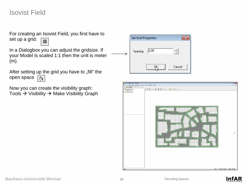
Isovist Field

For creating an Isovist Field, you first have to set up a grid: In a Dialogbox you can adjust the gridsize. If your Model is scaled 1:1 then the unit is meter (m). After setting up the grid you have to „fill“ the open space Now you can create the visibility graph: Tools Visibility Make Visibility Graph


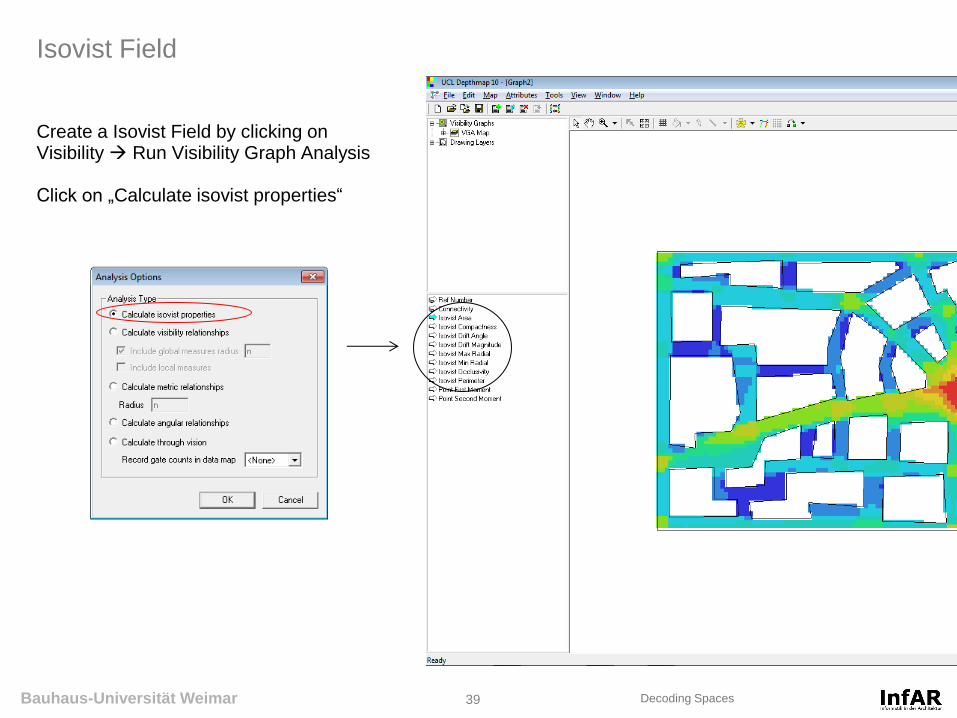
Isovist Field

Create a Isovist Field by clicking on Visibility Run Visibility Graph Analysis Click on „Calculate isovist properties“


Exercise - Isovist Field

Import „Campus.dxf“ Set Grid to 2 Fill the open space Calculate the isovist properties (Visibility Run Visibility Graph Analysis)


Visibility Graph

is a graph of mutually visible points in space In mathematical terms, a graph consists of two sets: the set of the vertices in the Graph and the set of edge connections joining pairs of vertices. The graph edges are undirected (that is, if v1 can see v2 , then v2 can see v1 ). (see Turner et al, 2001)

Schematic plan and visibility graph (from: Krämer & Kunze, 2005)


Visibility Graph

Create a Isovist Field by clicking on Visibility Run Visibility Graph Analysis Click on „Calculate visibility relationships“


Overview: Visibility Graph Measures

Connectivity gibt an wieviele Punkte im Raum mit einem Punkt verbunden sind (entspricht der Area eines Isovist) Integration gibt die durchschnittliche visuelle Distanz eines Punktes zu allen anderen Punkten an Clustering Coefficient

Control / Controllability Entropy / Relativised Entropy Intensity


Colour Range

Sometimes you have to adjust the color-range for making differences in the results visible more clearly.


Permeability / Visibility

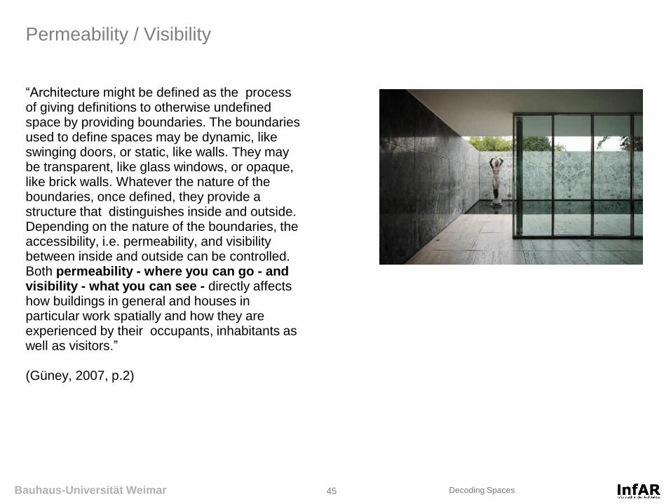
“Architecture might be defined as the process of giving definitions to otherwise undefined space by providing boundaries. The boundaries used to define spaces may be dynamic, like swinging doors, or static, like walls. They may be transparent, like glass windows, or opaque, like brick walls. Whatever the nature of the boundaries, once defined, they provide a structure that distinguishes inside and outside. Depending on the nature of the boundaries, the accessibility, i.e. permeability, and visibility between inside and outside can be controlled. Both permeability - where you can go - and visibility - what you can see - directly affects how buildings in general and houses in particular work spatially and how they are experienced by their occupants, inhabitants as well as visitors.” (Güney, 2007, p.2)


De-connecting Links in an Axial Map

When in an axial map 2 Lines intersect graphically, but are not connected in reality, as it is the case with bridges or tunnels, you have to de-connect the link(s) of the axial lines. Therefore press Unlink and click on the corresponding lines


Overview: Isovist Measures

Area Flächeninhalt des Sichtfeldes Perimeter Umfang des Sichtfeldes Occlusivity Länge der „verdeckten“ Kanten Compactness Verhältnis von Area zu Perimeter in Relation zur idealen Kreisform Drift Magnitude Distanz vom Blickpunkt zum „Schwerpunkt“ des Isovist-Polygons Drift Angle Winkel des Vektors (Blickpunkt zu Schwerpunkt) zur X-Achse Max Radial längster „Sichtstrahl“ Min Radial kürzester „Sichtstrahl“


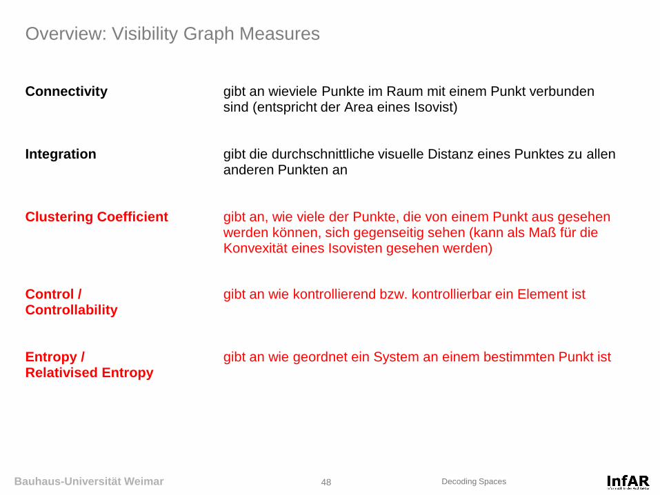
Overview: Visibility Graph Measures

Connectivity gibt an wieviele Punkte im Raum mit einem Punkt verbunden sind (entspricht der Area eines Isovist) Integration gibt die durchschnittliche visuelle Distanz eines Punktes zu allen anderen Punkten an Clustering Coefficient gibt an, wie viele der Punkte, die von einem Punkt aus gesehen werden können, sich gegenseitig sehen (kann als Maß für die Konvexität eines Isovisten gesehen werden)

Control / gibt an wie kontrollierend bzw. kontrollierbar ein Element ist Controllability Entropy / gibt an wie geordnet ein System an einem bestimmten Punkt ist Relativised Entropy


Clustering Coefficient

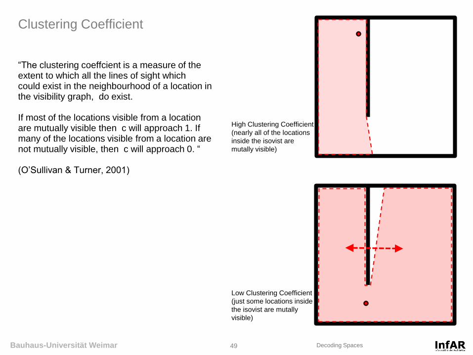
“The clustering coeffcient is a measure of the extent to which all the lines of sight which could exist in the neighbourhood of a location in the visibility graph, do exist. If most of the locations visible from a location are mutually visible then c will approach 1. If many of the locations visible from a location are not mutually visible, then c will approach 0. “ (O’Sullivan & Turner, 2001)

Low Clustering Coefficient

(just some locations inside

the isovist are mutally

visible)

High Clustering Coefficient

(nearly all of the locations

inside the isovist are

mutally visible)


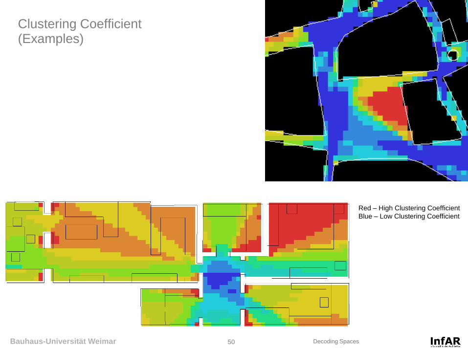
Clustering Coefficient (Examples)

Red – High Clustering Coefficient

Blue – Low Clustering Coefficient


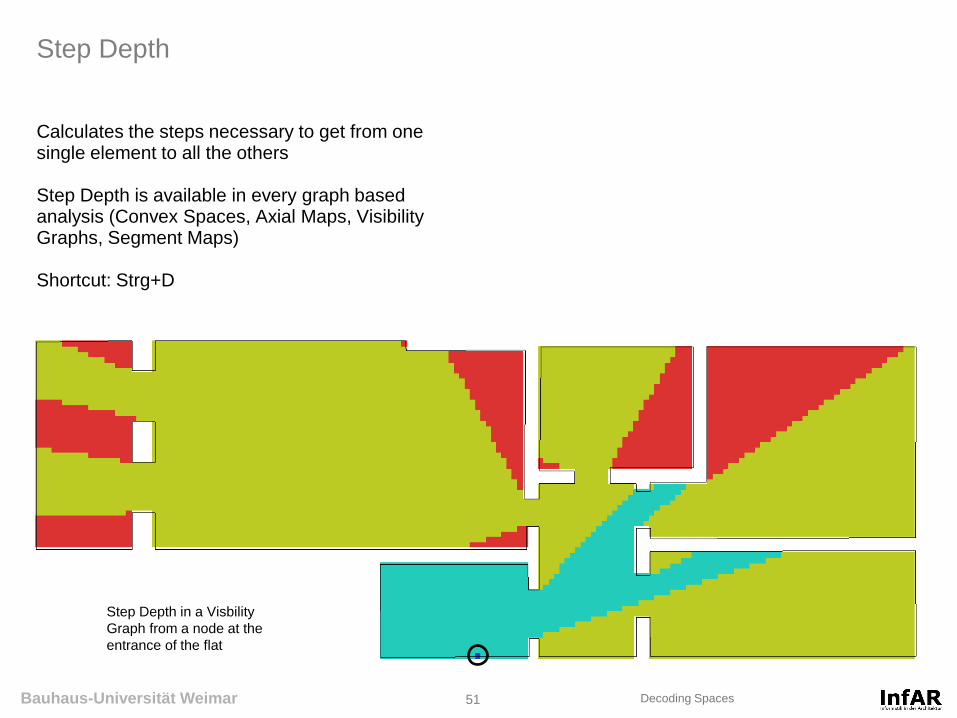
Step Depth

Calculates the steps necessary to get from one single element to all the others Step Depth is available in every graph based analysis (Convex Spaces, Axial Maps, Visibility Graphs, Segment Maps) Shortcut: Strg+D

Step Depth in a Visbility

Graph from a node at the

entrance of the flat


Control / Controllability

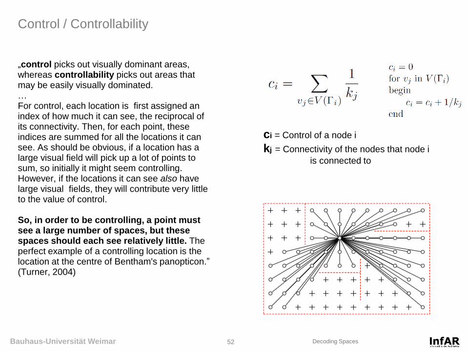
„control picks out visually dominant areas, whereas controllability picks out areas that may be easily visually dominated. … For control, each location is first assigned an index of how much it can see, the reciprocal of its connectivity. Then, for each point, these indices are summed for all the locations it can see. As should be obvious, if a location has a large visual field will pick up a lot of points to sum, so initially it might seem controlling. However, if the locations it can see also have large visual fields, they will contribute very little to the value of control. So, in order to be controlling, a point must see a large number of spaces, but these spaces should each see relatively little. The perfect example of a controlling location is the location at the centre of Bentham's panopticon.” (Turner, 2004)

ci = Control of a node i

kj = Connectivity of the nodes that node i

is connected to



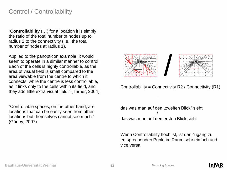
“Controllability (…) for a location it is simply the ratio of the total number of nodes up to radius 2 to the connectivity (i.e., the total number of nodes at radius 1). Applied to the panopticon example, it would seem to operate in a similar manner to control. Each of the cells is highly controllable, as the area of visual field is small compared to the area viewable from the centre to which it connects, while the centre is less controllable, as it links only to the cells within its field, and they add little extra visual field.” (Turner, 2004) “Controllable spaces, on the other hand, are locations that can be easily seen from other locations but themselves cannot see much.” (Güney, 2007)

Controllability = Connectivity R2 / Connectivity (R1)

=

das was man auf den „zweiten Blick“ sieht

/

das was man auf den ersten Blick sieht

Wenn Controllability hoch ist, ist der Zugang zu

entsprechenden Punkt im Raum sehr einfach und

vice versa.

/



„However, the panopticon is, of course, a contrived example. In reality, some spaces can be both controllable and controlling, and others uncontrollable and uncontrolling. It would seem an interesting avenue of research to see if anything further can be made from these measures, for example, to look at locations where crimes are committed, where a robber will want to control the victim, but at the same time be uncontrollable by the forces of law and order.” (Turner, 2004)

Control Controllability


Adding measures in Depthmap

Click on Attributes Add Column type in a name right-click on the new measure in the measures-list and chose edit

http://www.vr.ucl.ac.uk/depthmap/scripting/salascript.pdf

http://www.vr.ucl.ac.uk/depthmap/scripting/salascript.pdf


Integration in Segment Maps

Global Integration Local Integration (Bsp. R750) Integration-Choice Combination

(value("T1024 Node Count R750

metric")^2))/(value("T1024 Total Depth R750

metric")

value("T1024 Node Count")/value("T1024

Total Depth")

(value("T1024 Node Count")/value("T1024

Total Depth"))*(log(value("T1024

Choice")+2))


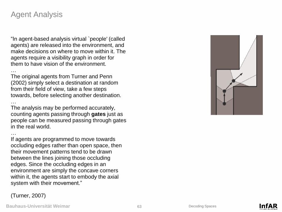
Agent Analysis

“In agent-based analysis virtual `people' (called agents) are released into the environment, and make decisions on where to move within it. The agents require a visibility graph in order for them to have vision of the environment. … The original agents from Turner and Penn (2002) simply select a destination at random from their field of view, take a few steps towards, before selecting another destination. … The analysis may be performed accurately, counting agents passing through gates just as people can be measured passing through gates in the real world. … If agents are programmed to move towards occluding edges rather than open space, then their movement patterns tend to be drawn between the lines joining those occluding edges. Since the occluding edges in an environment are simply the concave corners within it, the agents start to embody the axial system with their movement.” (Turner, 2007)


Agent Analysis in Depthmap

Tools Agent Analysis Run Agent Analysis (only available after a visibility graph is made)


New: Space Syntax in Grasshopper

See: “The parametric exploration of spatial properties – Coupling parametric geometry modeling and the graph-based spatial analysis of urban street networks” (Schneider, Bielik & König, 2012)

Figure 1. Designing is a cyclical process where artifacts are

created with the help of design tools (see Gänshirt, 2007)

Figure 2: Screenshot of Rhino, Grasshopper and the new

Spatial Analysis Components



Figure 3: Modular concept of the spatial analysis framework for Grasshopper

Figure 4. The ConvertToSegmentMap Component

converts geometric structures into segment maps Figure 5. Converting a segment map into a graph (for

details see Hillier & Iida, 2005)



Coupling Analysis & Modeling offers 2 important advantages:

1. Effectively comparing design variants

2. Using analyis results as parameters for the

parametric model

Figure 6. Three design variants deriving from a simple parametric

model, analysed in terms of betweenness (first row) and centrality

(second row)

Figure 7. Relating betweenness (choice) to

the width of streets

Figure 8. Relating centrality (integration) to the

height of buildings


Space Syntax Mailinglist

introduction to space syntax analysis software -...

Documents