Introduction to Spark

Outlines• A brief history of Spark• Programming with RDDs

Transformations Actions

A brief history

Limitations of MapReduce• MapReduce use cases showed two major limitations: 

Difficulty of programming directly in MapReduce Batch processing does not fit the use cases

Performance bottlenecks Data will be frequently loaded from and saved to hard drives

• Spark is designed to overpass the limitations of MapReduce Handles batch, interactive, and real‐time within a single framework Native integration with Java, Python, Scala Programming at a higher level of abstractionMore general: map/reduce is just one set of supported constructs

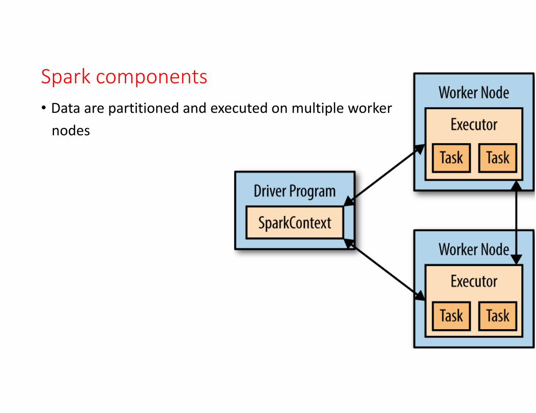
Spark components• Data are partitioned and executed on multiple workernodes

Resilient Distributed Dataset (RDD)• An RDD is simply a distributed collection of elements

An RDD is an immutable distributed collection of objects Each RDD is split into multiple partitions

• In Spark all work is expressed as one of three operations Creating new RDDs Transforming existing RDDs Calling operations on RDDs to compute a result

• Spark automatically distributes the data contained in RDDs across your cluster and parallelizes the operations you perform on them

Creation of an RDD• Users create RDDs in two ways

Loading an external dataset

Parallelizing a collection in your driver program

Transformations on RDDs• Transformations are operations on RDDs that return a new RDD

Such as map(), filter()

• Transformed RDDs are computed lazily Only when you use them in an action

• Creations of RDDs are also carried out lazily

Actions on RDDs• Operations that do something on the dataset• Operations that return a final value to the driver program or write data to an external storage system Such as count() and first()

• Actions force the evaluation of the transformations required for the RDD they were called on

Lazy evaluation• Lazy evaluation

The operation is not immediately performed when we call a transformation on an RDD

Spark internally records metadata to indicate that this operation has been requested

• Spark will not begin to execute until it sees an action• Spark will re‐compute the RDD and all of its dependencies each time we call an action on the RDD

• Result RDD will be computed twice in the above example

Persistence (caching)• Ask Spark to persist the data to avoid computing an RDD multiple times

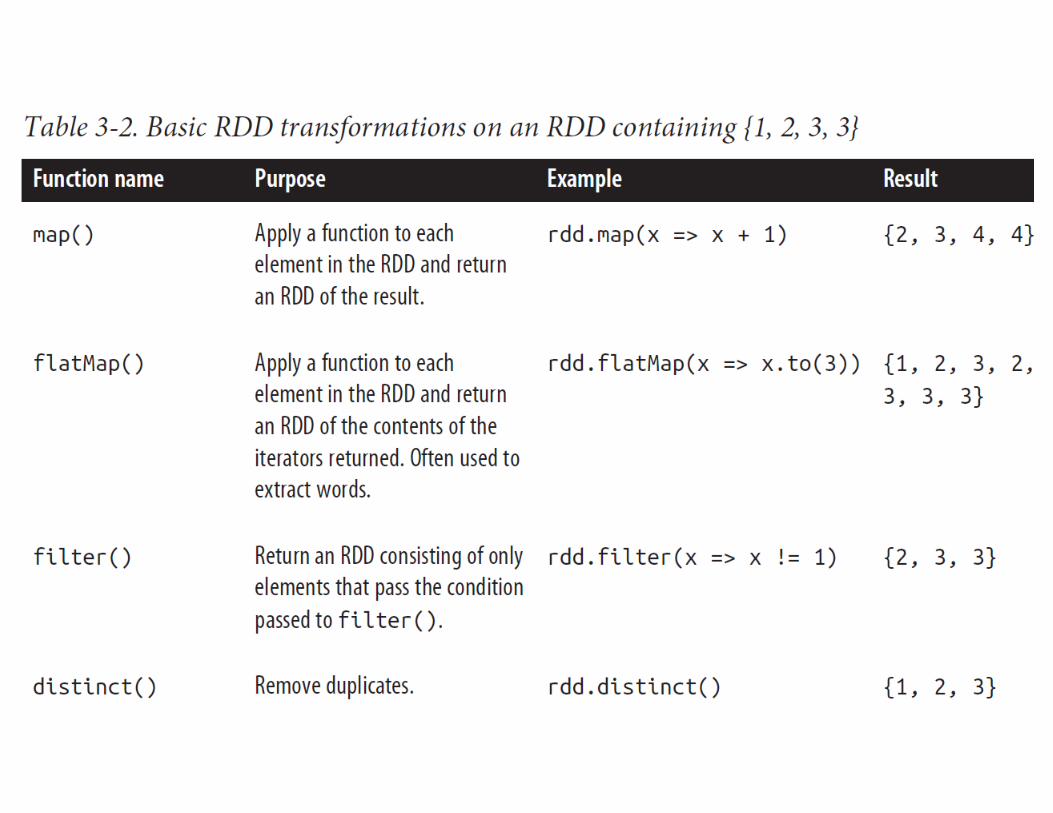
Element‐wise transformations• map()

Takes in a function and applies it to each element in the RDD with the result of the function being the new value of each element in the resulting RDD

map()’s return type does not have to be the same as its input type

• filter() Takes in a function and returns an RDD that only has elements that pass the filter() function

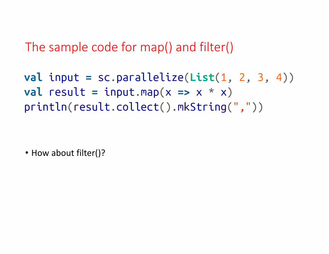
The sample code for map() and filter()

• How about filter()?

Element‐wise transformations• flatMap()

The function we provide to flatMap() is called individually for each element in our input RDD

Instead of returning a single element, we return an iterator with our return values

Rather than producing an RDD of iterators, we get back an RDD that consists of the elements from all of the iterators

flatMap() vs map()• flatMap(): “flattening” the iterators returned to it

Pseudo set operations

• union operation keeps duplicates• intersection operation removes duplicates

cartesian() transform

Actions

• countByValue() returns a map of each unique value to its count

• take(num): return the first num elements of the RDD• top() will use the default ordering on the data

• Both reduce() and fold() will reduce the input RDD to a single element of the same type fold() needs an initial value

• Each partition is processed sequentially using a single thread.• Partitions are processed in parallel using multiple executors / executor threads.• Final merge is performed sequentially using a single thread on the driver

More details on reduce() and fold()• RDD.reduce((x,y)=>x+y), RDD.fold(initial_value)((x,y)=>x+y)

x: accumulator y: item in the partition

• In reduce() The accumulator first takes the first element in a partition then updating its value by adding the next element

For example: a partition (1,2,3,4,5), RDD.reduce((x,y)=>x+y) Iteration 1: x=1, y=2 => x=(1+2)=3 Iteration 2: x=3, y=3 => x=(3+3)=6 Iteration 3: x=6, y=4 => x=(6+4)=10 Iteration 4: x=10, y=5 => x=(10+5)=15

• In fold() The accumulator first takes the initial value in a partition then updating its value by adding the next element

For example: a partition (1,2,3,4,5), RDD.fold(initial_value)((x,y)=>x+y) Iteration 1: x=0, y=1 => x=(0+1)=1

More details on reduce() and fold()• For multiple partitions of an RDD

First, the function will be applied on each partition.  Each partition will produce an accumulator

Then the function will be applied to the list of accumulators For fold(), the initial value will be used again when aggregating the accumulators

• The partitioning behavior, plus certain sources of ordering nondeterminism may bring uncertainty to fold() action when dealing with non communicative operations sc.parallelize(Seq(2.0, 3.0), 2).fold(1.0)((a, b) => pow(b, a)) What is the output?

aggregate()• The output of aggregate() can be different from the input RDD• Prototype:

def aggregate[B](z: ⇒ B)(seqop: (B, A) ⇒ B, combop: (B, B) ⇒ B): B aggregate(zeroValue) (seqOp, combOp) It traverses the elements in different partitions

Using seqOp to update the result Then applies combOp to results from different partitions

The zeroValue is used in both seqOp and combOp

• Example: how to calculate the average of an input RDD (1,2,3,3) val sum=inputRDD.aggregate(0)((x, y) => x + y, (x, y) => x + y) val count = inputRDD.aggregate(0)((x, y) => x + 1, (x, y) => x + y) val average=sum/count How about val count= inputRDD.aggregate(0)((x, y) => x + 1)?

aggregate()• Using a tuple x as the accumulator

x._1: the running total x._2: the running count