Introduction to Spectral Theory ofSchrodinger Operators

A. PankovDepartment of Mathematics

Vinnitsa State Pedagogical University21100 Vinnitsa

UkraineE-mail: pankov@e-math.ams.org

Contents

Preface 2

1 A bit of quantum mechanics 31.1 Axioms . . . . . . . . . . . . . . . . . . . . . . . . . . . . . . . 31.2 Quantization . . . . . . . . . . . . . . . . . . . . . . . . . . . 61.3 Heisenberg uncertainty principle . . . . . . . . . . . . . . . . . 81.4 Quantum oscillator . . . . . . . . . . . . . . . . . . . . . . . . 9

2 Operators in Hilbert spaces 132.1 Preliminaries . . . . . . . . . . . . . . . . . . . . . . . . . . . 132.2 Symmetric and self-adjoint operators . . . . . . . . . . . . . . 152.3 Examples . . . . . . . . . . . . . . . . . . . . . . . . . . . . . 172.4 Resolvent . . . . . . . . . . . . . . . . . . . . . . . . . . . . . 22

3 Spectral theorem of self-adjoint operators 243.1 Diagonalization of self-adjoint operators . . . . . . . . . . . . 243.2 Spectral decomposition . . . . . . . . . . . . . . . . . . . . . . 273.3 Functional calculus . . . . . . . . . . . . . . . . . . . . . . . . 313.4 Classification of spectrum . . . . . . . . . . . . . . . . . . . . 33

4 Compact operators and the Hilbert-Schmidt theorem 354.1 Preliminaries . . . . . . . . . . . . . . . . . . . . . . . . . . . 354.2 Compact operators . . . . . . . . . . . . . . . . . . . . . . . . 364.3 The Hilbert-Schmidt theorem . . . . . . . . . . . . . . . . . . 374.4 Hilbert-Schmidt operators . . . . . . . . . . . . . . . . . . . . 394.5 Nuclear operators . . . . . . . . . . . . . . . . . . . . . . . . . 424.6 A step apart: polar decomposition . . . . . . . . . . . . . . . . 444.7 Nuclear operators II . . . . . . . . . . . . . . . . . . . . . . . 454.8 Trace and kernel function . . . . . . . . . . . . . . . . . . . . 49

5 Perturbation of discrete spectrum 515.1 Introductory examples . . . . . . . . . . . . . . . . . . . . . . 515.2 The Riesz projector . . . . . . . . . . . . . . . . . . . . . . . . 525.3 The Kato lemma . . . . . . . . . . . . . . . . . . . . . . . . . 535.4 Perturbation of eigenvalues . . . . . . . . . . . . . . . . . . . . 55

6 Variational principles 596.1 The Glazman lemma . . . . . . . . . . . . . . . . . . . . . . . 596.2 The minimax principle . . . . . . . . . . . . . . . . . . . . . . 64

1

7 One-dimensional Schrodinger operator 677.1 Self-adjointness . . . . . . . . . . . . . . . . . . . . . . . . . . 677.2 Discreteness of spectrum . . . . . . . . . . . . . . . . . . . . . 727.3 Negative eigenvalues . . . . . . . . . . . . . . . . . . . . . . . 75

8 Multidimensional Schrodinger operator 818.1 Self-adjointness . . . . . . . . . . . . . . . . . . . . . . . . . . 818.2 Discrete spectrum . . . . . . . . . . . . . . . . . . . . . . . . . 888.3 Essential spectrum . . . . . . . . . . . . . . . . . . . . . . . . 908.4 Decay of eigenfunctions . . . . . . . . . . . . . . . . . . . . . . 938.5 Agmon’s metric . . . . . . . . . . . . . . . . . . . . . . . . . . 95

9 Periodic Schrodinger operators 999.1 Direct integrals and decomposable operators . . . . . . . . . . 999.2 One dimensional case . . . . . . . . . . . . . . . . . . . . . . . 1019.3 Multidimensional case . . . . . . . . . . . . . . . . . . . . . . 1049.4 Further results . . . . . . . . . . . . . . . . . . . . . . . . . . 1069.5 Decaying perturbations of periodic potentials . . . . . . . . . . 108

References 110

2

Preface

Here are lecture notes of the course delivered at the Giessen University dur-ing my visit as DFG guest professor (1999-2000 teaching year). The audi-ence consisted of graduate and PhD students, as well as young researchersin the field of nonlinear analysis, and the aim was to provide them witha starting point to read monographs on spectral theory and mathematicalphysics. According to introductory level of the course, it was required astandard knowledge of real and complex analysis, as well as basic facts fromlinear functional analysis (like the closed graph theorem). It is desired, butnot necessary, some familiarity with differential equations and distributions.The notes contain simple examples and exercises. Sometimes we omit proofs,or only sketch them. One can consider corresponding statements as prob-lems (not always simple). Remark also that the second part of Section 9 isnot elementary. Here I tried to describe (frequently, even without rigorousstatements) certain points of further development. The bibliography is veryrestricted. It contains few books and survey papers of general interest (withonly one exception: [9]).It is a pleasant duty for me to thank Thomas Bartsch who initiated my

visit and the subject of course, as well as all the members of the MathematicalInstitute of Giessen University, for many interesting and fruitful discussions.Also, I am grateful to Petra Kuhl who converted my handwritten draft intoa high quality type-setting.

3

1 A bit of quantum mechanics

1.1 Axioms

Quantum mechanics deals with microscopic objects like atoms, molecules,etc. Here, as in any physical theory, we have to consider only those quantitieswhich may be measured (at least in principle). Otherwise, we go immediatelyto a kind of scholastic. Physical quantities, values of which may be foundby means of an experiment (or measured) are called observables. It turnsout to be that in quantum mechanics it is impossible, in general, to predictexactly the result of measurement. This result is a (real) random variableand, in fact, quantum mechanics studies lows of distribution of such randomvariables.Now we discuss a system of axioms of quantum mechanics suggested by

J. von Neumann.

Axiom 1.1. States of a quantum system are nonzero vectors of a complexseparable Hilbert space H, considered up to a nonzero complex factor. Thereis a one-to-one correspondence between observable and linear self-adjoint op-erators in H. In what follows we consider states as unit vectors in H.If a is an observable, we denote by a the corresponding operator. We

say that observables a1, . . . , an are simultaneously measurable if their valuesmay be measured up to an arbitrarily given accuracy in the same experiment.This means that for an arbitrary state ψ ∈ H the random variables a1, . . . , anhave a simultaneous distribution function Pψ(λ1, . . . ,λn), i.e. Pψ(λ1, . . . ,λn)is a probability that the values of observables a1, . . . , an measured in the stateψ are less or equal to λ1, . . . ,λn, respectively.

Axiom 1.2. Observables a1, . . . , an are simultaneously measurable if and onlyif the self-adjoint operators a1, . . . , an mutually commutes. In this case

(1.1) Pψ(λ1, . . . ,λn) = E(1)λ1E(2)λ2. . . E

(n)λn

ψ 2,

where E(k)λ is the spectral decomposition of unit corresponding to the operator

ak.

It is clear that the right-hand side of (1.1) depends on the state itself, noton representing unit vector ψ (ψ is defined up to a complex factor ζ, |ζ = 1).Also this expression does not depend on the order of observables, since thespectral projectors E

(k)λ commute.

Among all observables there is one of particular importance: the energy.Denote by H the corresponding operator. This operator is called frequently

4

the (quantum) Hamiltonian, or the Schrodinger operator. It is always as-sumed that H does not depend explicitly on time.

Axiom 1.3. There exists a one parameter group Ut of unitary operators(evolution operator) that map an initial state ψ0 at the time t = 0 to thestate ψ(t) = Utψ0 at the time t. The operator Ut is of the form

(1.2) Ut = e− ihtH ,

where h is the Plank constant. If ψ0 ∈ D(H), the domain of H, then theH−valued function ψ(t) is differentiable and

(1.3) ihdψ(t)

dt= Hψ(t).

Thus, the evolution of quantum systems is completely determined by itsHamiltonian H. Equation (1.3) is called the Schrodinger equation.

Axiom 1.4. To each non-zero vector of H it corresponds a state of quantumsystem and every self-adjoint operator in H corresponds to an observable.

The last axiom is, in fact, too strong and sometimes one needs to weakenit. However, for our restricted purpose this axiom is sufficient.Now let us discuss some general consequences of the axioms. Let a be

an observable and a the corresponding self-adjoint operator with the domainD(a). We denote by aψ the mean value, or mathematical expectation, of theobservable a at the state ψ.If ψ ∈ D(a), then the mean value aψ exists and

(1.4) aψ = (aψ,ψ).

Indeed, due to the spectral theorem

(aψ,ψ) =∞

−∞λd(Eλψ,ψ)

However,(Eλψ,ψ) = (E

2λ,ψ,ψ) = (Eλψ, Eλψ) = Eλψ

2.

Using (1.1), we see that

(aψ,ψ) =∞

−∞λd Eλψ

2 =∞

−∞λdPψ(λ) = aψ.

Denote by δψa the dispersion of a at the state ψ, i.e. the mean value of(a− aψ)2.

5

The dispersion δψa exists if ψ ∈ D(a). In this case

(1.5) δψa = aψ − aψψ 2.

The first statement is a consequence of the spectral theorem (consider it asan exercise). Now consider a self-adjoint operator (a− aψI)2, where I is theidentity operator. Applying (1.4) to this operator, we have

δψa = ((a− aψI)2ψ,ψ) = ((a− aψI)ψ, (a− aψI)ψ) = aψ − aψ 2.

Now we have the following important

Claim 1.5. An observable a takes at a state ψ a definite value λ with prob-ability 1 if and only if ψ is an eigenvector of a with the eigenvalue λ.

Indeed, if a takes at ψ the value λ with probability 1, then aψ = λ andδψa = 0. Hence, by (1.5), aψ − λψ = 0, i. e. aψ = λψ. Conversely,if aψ = λψ, then (1.4) implies that aψ = (aψ,ψ) = λ(ψ,ψ) = λ. Hence,δψ = aψ − aψψ 2 = aψ − λψ 2 = 0.Consider a particular case a = H. Assume that at the time t = 0 the

state of our system is an eigenvector ψ0 of H with the eigenvalue λ0. Then

ψ(t) = e−iλ0t/hψ0

solves the Schrodinger equation. However, ψ(t), differs from ψ0 by a scalarfactor and, hence, define the same state as ψ0. Assume now that Utψ0 =c(t)ψ0. The function c(t) = (Utψ0,ψ0) is continuous, while the group lowUt+s = UtUs implies that c(t + s) = c(t)c(s). Hence, c(t) is an exponentialfunction. Therefore, it is differentiable and

Hψ0 = ihd

dtUtψ0|t=0 = λ0ψ0,

with λ0 = ihdc(t)dt|t=0.

Thus, the state of quantum system is a stationary state, i. e. it doesnot depend on time, if and only if it is represented by an eigenvector of theHamiltonian. The equation

Hψ = λψ

for stationary states is called stationary Schrodinger equation.

6

1.2 Quantization

Let us consider a classical dynamical systems, states of which are definedby means of (generalized) coordinates q1, . . . , qn and (generalized) impulsesp1, . . . , pn. Assume that the (classical) energy of our system is defined by

(1.6) Hcl =n

k=1

p2k2mk

+ v(q1, . . . , qn),

where mk are real constants, qk ∈ R, pk ∈ R. A typical example is thesystem of l particles with a potential interaction. Here n = 3l, the number ofdegrees of freedom, q3r−2, q3r−1, q3r are Cartesian coordinates of rth particle,p3r−2, p3r−1, p3r are the components of corresponding momentum, m3r−2 =m3r−1 = m3r is the mass of rth particle, and v(q1, q2, . . . , qn) is the potentialenergy.There is a heuristic rule of construction of corresponding quantum system

such that the classical system is, in a sense, a limit of the quantum one. Asthe space of states we choose the space L2(Rn) of complex valued functionsof variables q1, . . . , qn. To each coordinate qk we associate the operator qk ofmultiplication by qk

(qkψ)(q1, . . . , qn) = qkψ(q1, . . . , qn).

Exercise 1.6. Let h(q1, . . . , qn) be a real valued measurable function. Theoperator h defined by

(hψ)(q1, . . . , qn) = h(q1, . . . , qn)ψ(q1, . . . , qn),

D(h) = ψ ∈ L2(Rn) : h(q)ψ(q) ∈ L2(Rn),is self-adjoint.Thus, qk is a self-adjoint operator. We set also

pk =h

i

∂

∂qk,

with

D(pk) = ψ(q) ∈ L2(Rn) : ∂ψ∂qk∈ L2(Rn),

where ∂ψ/∂qk is considered in the sense of distributions.

Exercise 1.7. Show that pk is a self-adjoint operator.

7

Now we should define the quantum Hamiltonian as a self-adjoint operatorgenerated by the expression

(1.7) H = −h2

2

n

k=1

1

mk

∂2

∂q2k+ v(q1, . . . , qn).

However, at this point some problems of mathematical nature arise. Roughlyspeaking, what does it mean operator (1.7)? It is easy to see that operator(1.7) is well-defined on the space C∞0 (Rn) of smooth finitely supported func-tions and is symmetric. So, the first question is the following. Does thereexist a self-adjoint extension of operator (1.7) with C∞0 (Rn) as the domain?If no, there is no quantum analogue of our classical system. If yes, then howmany of self-adjoint extensions do exist? In the case when there are differentself-adjoint extensions we have different quantum versions of our classicalsystem. In good cases we may except that there exists one and only oneself-adjoint operator generated by (1.7). It is so if the closure of H definedfirst on C∞0 (Rn) is self-adjoint. In this case we say that H is essentiallyself-adjoint on C∞0 (Rn).By means of direct calculation one can verify that the operators of im-

pulses and coordinates satisfy the following Heisenberg commutation rela-tions

(1.8) [pk, qk] =h

iI, [pk, qj] = 0, k = j.

In fact, these relations are easy on C∞0 (Rn), but there are some difficultiesconnected with the rigorous sense of commutators in the case of unboundedoperators. We do not go into details here. Remark that there is essentiallyone set of operators satisfying relations (1.8). In the classical mechanicscoordinates and impulses are connected by relations similar to (1.8), butwith respect to the Poisson brackets. In our (coordinate) representationof quantum system with Hamiltonian (1.7) a state is given by a functionψ(q1, . . . , qn, z) with belongs to L

2(Rn) for every fixed time t. Moreover,

ψ(q1, . . . , qn, t) = e− ihtHψ(q1, . . . , qn, 0)

The Schrodinger equation is now of the form

ih∂ψ

∂t= −h

2

2

n

k=1

1

mk

∂2ψ

∂q2k+ v(q1, . . . , qn)ψ.

The function ψ(q1, . . . , qn, t) is called a wave function of the quantum sys-tem. (The same term is used frequently for functions ψ(q1, . . . , qn) ∈ L2(Rn)representing states of the system).

8

Let E(k)λ be a decomposition of identity for qk,

qk =∞

−∞λdE

(k)λ .

Then E(k)λ is just the operator of multiplication by the characteristic function

of the setq = (q1, . . . , qn) ∈ Rn : qk ≤ λ

Hence the simultaneous distribution of q1, . . . , qn is given by

Pψ(λ1, . . . ,λn) =λ1

−∞. . .

λn

−∞|ψ(q1, . . . , qn)|2dq1 . . . dqn.

Therefore, the square of modulus of a wave function is exactly thedensity of simultaneous distribution of q1, . . . , qn. Thus, the probabilitythat a measurement detects values of coordinates q1, . . . , qn in the intervals(a1, b1), . . . , (an, bn) respectively is equal to

b1

a1

. . .bn

an

|ψ(q1, . . . , qn)|2dq1, . . . , dqn.

We have just described the so-called coordinate representation which is, ofcourse, not unique. There are other representations, e. g. so-called impulserepresentation (see [1] for details).We have considered quantization of classical systems of the form (1.6).

For more general classical systems quantization rules are more complicated.In addition, let us point out that there exist quantum systems which cannotbe obtained from classical ones by means of quantization, e.g. particles withspin.

1.3 Heisenberg uncertainty principle

Let us consider two observables a and b, with corresponding operators a andb. Let ψ be a vector such that (ab− ba)ψ makes sense. The uncertainties ofthe results of measurement of a and b in the state ψ are just

∆a = ∆ψa = δψa = aψ − aψψ∆b = ∆ψb = δψb = bψ − bψψ .

We have

(1.9) ∆a∆b ≥ 12|((ab− ba)ψ,ψ)|

9

Indeed, let a1 = a− aψI, b1 = b− bψI. Then a1b1 − b1a1 = ab− ba. Hence,

|((ab− ba)ψ,ψ)| = |((a1b1 − b1a1)ψ,ψ)|= |(a1b1ψ,ψ)− (b1a1ψ,ψ)| = |(b1ψ, a1ψ)− (a1ψ, b1ψ)|= 2|Im(a1ψ, b1ψ)| ≤ 2|(a1ψ, b1ψ)| ≤ 2 a1ψ b1ψ

= 2 aψ − aψψ bψ − bψψ = 2∆a∆b.We say that the observables a and b are canonically conjugate if

ab− ba = h

iI

In this case the right hand part of (1.8) is independent of ψ and

(1.10) ∆a∆b ≥ h/2

It is so for the components qk and pk of coordinates and momenta, and, asconsequence, we get the famous Heisenberg uncertainly relations

(1.11) ∆pk∆qk ≥ h/2.

Due to Axiom 1.2, two observables are simultaneously measurable if thecorresponding operators commute. Relation (1.11) gives us a quantitativeversion of this principle. If an experiment permits us to measure the coordi-nate qk with a high precision, then at the same experiment we can measurethe corresponding impulse pk only very roughly: the accuracies of these twomeasurements are connected by (1.11).

1.4 Quantum oscillator

The classical (1-dimensional) oscillator is a particle with one degree of free-dom which moves in the potential field of the form

v(x) =ω2

2x2, x ∈ R.

The classical energy is of the form

Mcl =m

2(x)2 +

mω2

2x2 =

p2

2m+mω2

2x2,

where m is the mass of the particle, and p = mx is its momentum.

10

The space of states of the quantum analogue is H = L2(R), the oper-ators of coordinate and momentum were defined above, and the quantumHamiltonian H is a self-adjoint operator generated by the expression

− h

2m

d2

dx2+mω2

2x2.

For the sake of simplicity we set h = m = ω = 1. Then

H =1

2(− d

2

dx2+ x2).

Let H be a linear subspace of L2(R) (not closed!) that consists of all functionsof the form

P (x)e−x2

2 ,

where P (x) is a polynomial.

Exercise 1.8. H is dense in L2(R).

Now let us introduce the so-called operators of annihilation and birth.

A =1√2(x+ ip) , A∗ =

1√2(x− 1p)

In fact, one can show that A∗ is the adjoint operator to A, defined on H.However, we do not use this fact. So, one can consider A∗ as a single symbol.These operators, as well as p, x and H, are well-defined on the space H andmap H into itself (verify this). As consequence, on the space H products andcommutators of all these operators are also well-defined. Verify the followingidentities (on H):

(1.12) [A,A∗] = I,

(1.13) H = A∗A =1

2I = AA∗ − 1

2I,

(1.14) [H,A]−A , [H,A∗] = A∗

Exercise 1.9. Let ψ ∈ H be an eigenvector of H with the eigenvalue λ andA∗ψ = 0. Then A∗ψ is an eigenvector of H with the eigenvalues λ+ 1.

11

Now let

ψ0(x) = e−x2

2

Then

Hψ0 =1

2ψ0,

and ψ0 ∈ H is an eigenvector of H with the eigenvalue 12(verify!). Let us

define vectors ψk ∈ H by

ψk+1 =√2A∗ψk,

or

ψk = (√2A∗)kψ0.

Exercise 1.10. Hψk = (k +12)ψk.

Hence, ψk is an eigenvector of H with the eigenvalue (k + 12). Since

ψk ∈ H, we haveψk(x) = Hk(x)e

−x2

2 ,

where Hk(x) are polynomials (the so-called Hermite polynomials). The func-tions ψk are said to be Hermite functions.

Exercise 1.11. Calculate (Hψk,ψl) and verify that ψk is an orthogonalsystems in L2(R) (not normalized).

Exercise 1.12. Show that the system ψk may be obtained by means oforthogonalization of the system

xne−x2

2 .

Exercise 1.13. Verify the following identities

Hn(x) = (−1)nex2 dn

dxne−x

2

,

dnHndxn

= 2n · n! ,Hn+1(x) = 2xHn(x)− 2nHn−1(x) .

Calculate H0(x), H1(x), H2(x), H3(x) and Hn(x).

Exercise 1.14. Show that ψk is an orthogonal basis in L2(R). Moreover,ψk

2 = 2k · k!√π.

12

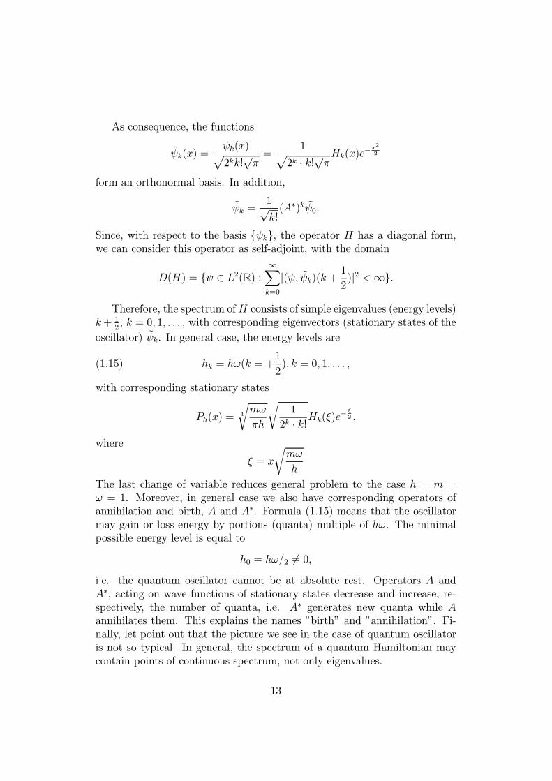
As consequence, the functions

ψk(x) =ψk(x)

2kk!√π=

1

2k · k!√πHk(x)e−x2

2

form an orthonormal basis. In addition,

ψk =1√k!(A∗)kψ0.

Since, with respect to the basis ψk, the operator H has a diagonal form,we can consider this operator as self-adjoint, with the domain

D(H) = ψ ∈ L2(R) :∞

k=0

|(ψ, ψk)(k + 12)|2 <∞.

Therefore, the spectrum ofH consists of simple eigenvalues (energy levels)k+ 1

2, k = 0, 1, . . . , with corresponding eigenvectors (stationary states of the

oscillator) ψk. In general case, the energy levels are

(1.15) hk = hω(k = +1

2), k = 0, 1, . . . ,

with corresponding stationary states

Ph(x) =4mω

πh

1

2k · k!Hk(ξ)e− ξ2 ,

where

ξ = xmω

h

The last change of variable reduces general problem to the case h = m =ω = 1. Moreover, in general case we also have corresponding operators ofannihilation and birth, A and A∗. Formula (1.15) means that the oscillatormay gain or loss energy by portions (quanta) multiple of hω. The minimalpossible energy level is equal to

h0 = hω/2 = 0,

i.e. the quantum oscillator cannot be at absolute rest. Operators A andA∗, acting on wave functions of stationary states decrease and increase, re-spectively, the number of quanta, i.e. A∗ generates new quanta while Aannihilates them. This explains the names ”birth” and ”annihilation”. Fi-nally, let point out that the picture we see in the case of quantum oscillatoris not so typical. In general, the spectrum of a quantum Hamiltonian maycontain points of continuous spectrum, not only eigenvalues.

13

2 Operators in Hilbert spaces

2.1 Preliminaries

To fix notation, we recall that a Hilbert space H is a complex linear spaceequipped with an inner product (f, g) ∈ C such that

(f, g, ) = (g, f),

(λ, f1 + λ2f2, g) = λ1(f1, g) + λ2(f2, g),

(f,λ, g1 + λ2g2) = λ1(f, g1) + λ2(f, g2),

where λ1,λ2 ∈ C and¯stands for complex conjugation,

(f, f) ≥ 0, f ∈ H,

(f, f) = 0 iff f = 0. Such inner product defines a norm

f = (f, f)1/2

and, by definition, H is complete with respect to this norm.

Exercise 2.1. Prove the following polarization identity

(f, g) =1

4[(f + g, f + g)− (f − g, f − g)

+ i(f + ig, f + ig)− i(f − ig, f − ig)]

for every f, g ∈ H.Let H1 and H2 be two Hilbert spaces. By definition, a linear operator

A : H1 → H2 is a couple of two objects:

- a linear (not necessary dense, or closed) subspace D(A) ⊂ H1 which iscalled the domain of A;

- a linear map A : D(A)→ H2.

We use the following notations

kerA = f ∈ D(A) : Af = 0,imA = g ∈ H2 : g = Af, f ∈ D(A)

for kernel and image of A respectively. (Distinguish imA and Imλ, theimaginary part of a complex number.)

14

The operator A is said to be bounded (or continuous), if there exists aconstant C > 0 such that

(2.1) Af ≤ C f , f ∈ D(A).The norm A of A is defined as the minimal possible C in (2.1), or

(2.2) A = supf∈D(A),f=0

Af

f.

In this case A can be extended by continuity to the closure D(A) of D(A).Usually, we deal with operators defined on dense domains, i.e. D(A) = H1.If such an operator is bounded, we consider it to be defined on the wholespace H1.If kerA = 0, we define the inverse operator A−1 : H2 → H1 in the

following way: D(A−1) = imA and for every g ∈ imA we set A−1g = f ,where f ∈ D(A) is a (uniquely defined) vector such that g = Af .Let A : H1 → H2 and B : H2 → H3 be linear operators. Their product

(or composition) BA : H1 → H3 is defined by

D(BA) = f ∈ D(A) : Af ∈ D(B), (BA)f = B(Af), f ∈ D(BA).Certainly, it is possible that imA∩D(B) = 0. In this case D(BA) = 0.The sum of A : H1 → H2 and A2 : H1 → H2 is an operator A1 + A2 :

H1 → H2 defined by

D(A1 +A2) = D(A1) ∩D(A2),(A1 +A2)f = A1f +A2f.

Again, the case D(A1 +A2) = 0 is possible.Let A : H1 → H2 be a linear operator. By definition the graph G(A) of A

is a linear subspace of H1⊕H2 consisting of all vectors of the form f,Af,f ∈ D(A).Exercise 2.2. A linear subspace of H1⊕H2 is the graph of a linear operatorif it does not contain vectors of the form 0, g with g = 0.A linear operator A : H1 → H2 is said to be closed if its graph G(A)

is a closed subspace of H1 × H2. A is called closable if G(A) is the graphof some operator A. In this case A is called the closure of A. Equivalently,A : H1 → H2 is closed if fn ∈ D(A), fn → f in H1 and Afn → g in Himply f ∈ D(A) and Af = g. A is closable if fn ∈ D(A), fn → 0 in H1 andAfn → g in H2 imply g = 0.Now let us list some simple properties of such operators.

15

• Every bounded operator A is closable. Such an operator is closed pro-vided D(A) is closed.

• If A is closed, then kerA is a closed subspace of H1.

• If A is closed and kerA = 0, then A−1 is a closed operator.Let A1, A2 : H1 → H2 be two linear operators. We say that A2 is an extensionof A1 (in symbols A1 ⊂ A2) if D(A1) ⊂ D(A2) and A2f = A1f , f ∈ D(A1).Obviously, the closure A of A (if it exists) is an extension of A.

2.2 Symmetric and self-adjoint operators

First, let us recall the notion of adjoint operator. Let A : H1 → H2 be alinear operator such that D(A) = H1 (important assumption!). The adjointoperator A∗ : H2 → H1 is defined as follows. The domain D(A

∗) of A∗

consists of all vectors g ∈ H2 with the following property:

there exists g∗ ∈ H∗1 such that (Af, g) = (f, g∗) ∀f ∈ D(A).Since D(A) is dense in H1, the vector g

∗ is uniquely defined, and we set

A∗g = g∗

In particular, we have

(Af, g) = (f,A∗g), f ∈ D(A), g ∈ D(A∗).

Evidently, g ∈ D(A∗) iff the linear functional l(f) = (Af, g) defined onD(A) is continuous. Indeed, in this case on can extend l to D(A) = H1 bycontinuity. Then, by the Riesz theorem, we have l(f) = (Af, g) = (f, g∗) forsome g∗ ∈ H1.Let us point out that the operation ∗ of passage to the adjoint operator

reverses arrows: if A : H1 → H2, then A∗ : H2 → H1. In the language of the

theory of categories this means that ∗ is a contravariant functor.Now we list a few simple properties of adjoint operators.

• If A1 ⊂ A2, then A∗2 ⊂ A∗1.• If A is bounded and D(A) = H1, then D(A2) = H2 and A

∗ is bounded.Moreover, A∗ = A .

• For every linear operator A, with D(A) = H1, A∗ is a closed operator.

16

If E is a linear subspace of H, we denote by E⊥ the orthogonal comple-ment of E, i.e.

E⊥ = g ∈ H : (f, g) = 0 ∀f ∈ E.Evidently,E⊥ is a closed subspace of H, and E⊥ = (E)⊥.Exercise 2.3. (i) kerA∗ = (imA)⊥.

(ii) Operators (A∗)−1 and (A−1)∗ exist iff kerA = 0 and imA is dense inH2.

(iii) In the last case, (A∗)−1 = (A−1)∗.

Proposition 2.4. D(A∗) is dense in H2 iff A is closable. In this case A =A∗∗ = (A∗)∗.

Proof. By definition of H1 ⊕H2,

(f1, g1, f2, g2) = (f1, f2) + (g1, g2).Now we have easily that g, g∗ ∈ G(A∗) iff g∗,−g ⊥ G(A) (prove!). Thismeans that the vectors A∗g,−g form the orthogonal complement of G(A).Hence, G(A) is the orthogonal complement to the space of all vectors of theform A∗g,−g.The space D(A∗) is not dense in H2 if and only if there exists a vector

h ∈ H2 such that h = 0 and h ⊥ D(A∗), or, which is the same, 0, h ⊥A∗g,−g for all g ∈ D(A∗). The last means that 0, h ∈ G(A), i.e. G(A)cannot be a graph of an operator and, hence, A is not closable.The last statement of the proposition is an exercise. (Hint: G(A∗∗) =

G(A)).

Now we will consider operators acting in the same Hilbert space H(H =H1 = H2). Let A : H → H be an operator with dense domain, D(A) = H.We say that A is symmetric if A ⊂ A∗, i.e.

(Af, g) = (f,Ag) ∀f, g ∈ D(A).First, we remark that every symmetric operator is closable. Indeed, we haveG(A) ⊂ G(A∗). Since A∗ is closed, (i.e. G(A∗) = G(A∗)), we see thatG(A) ⊂ G(A∗) = G(A∗). Hence, G(A) does not contain any vector of theform 0, h, h = 0. Therefore, G(A) is the graph of an operator. It is easyto see that the closure A of symmetric operator A is a symmetric operator.An operator A : H→ H is said to be self-adjoint if A = A∗. If A is self-

adjoint, we say that A is essentially self-adjoint. Each self-adjoint operatoris obviously closed. If A is self-adjoint and there exists A−1, then A−1 isself-adjoint. Indeed, (A−1)∗ = (A∗)−1 = A−1.

17

Proposition 2.5. A closed symmetric operator A is self-adjoint if and onlyif A∗ is symmetric.

Proof. We prove the first statement only. If A is closed, then, due to Proposi-tion 2.4, A∗∗ = A. Since A∗ is symmetric, we have A∗ ⊂ A∗∗ = A. However,A itself is symmetric: A ⊂ A∗. Hence, A ⊂ A∗ ⊂ A and we conclude.Exercise 2.6. An operatorA with the dense domain is essentially self-adjointif and only if A∗ and A∗∗ are well-defined, and A∗ = A∗∗.

Theorem 2.7. An operator A such that D(A) = H is essentially self-adjointiff there is one and only one self-adjoint extension of A.

The proof is not trivial and based on the theory of extension of symmetricoperators. It can be found, e.g., in [8].

2.3 Examples

We consider now a few examples.

Example 2.8. Let J be an interval of real line, not necessary finite and a(x)a real valued measurable function which is finite almost everywhere. Let Abe the operator of multiplication by a(x) defined by

D(A) = f ∈ L2(J) : af ∈ L2(J),(Af)(x) = a(x)f(x).

Then A is a self-adjoint operator. To verify this let us first prove thatD(A) =L2(J). Let g ∈ L2(J) be a function such that

J

fgdx = 0 ∀f ∈ D(A).

We show that g = 0. With this aim, given N > 0 we consider the set

JN = x ∈ J : |a(x)| < N.

Since a(x) is finite almost everywhere, we have

meas(J \ ∪∞N=1JN ) = 0.

Hence, it suffices to prove that g|JN = 0 for all integer N . Let χN be thecharacteristic function of JN , i.e. χN = 1 on JN and χN = 0 on J \ JN . Forevery f ∈ L2(J) we set fN = χNf .

18

Then, obviously, fN ∈ L2(J) and afN ∈ L2(J). Therefore, for all f ∈L2(J) we have

JN

fgdx =J

fNgdx = 0.

If we take here f = g, we get

JN

ggdx =JN

|g|2dx = 0,

and, hence, g = 0 on JN .Now, let g ∈ D(A∗), i.e. there exists g∗ ∈ L2(J) such that

J

afgdx =J

fg∗dx ∀f ∈ D(A).

If we take as f an arbitrary function in L2(J) vanishing outside JN , we see asabove that ag = g∗ almost everywhere, i.e. g ∈ D(A). Hence, D(A∗) = D(A)and A∗g = Ag, i.e. A = A∗.

To consider next examples we need some information on weak derivatives(see, e.g., [6], [8]). Let f ∈ L2(J). Recall that a function g ∈ L2(J) is saidto be the weak derivative of f if

(2.3)J

gϕdx = −J

fϕ dx ∀ϕ ∈ C∞0 (J).

In this case we write g = f . For any integer m we set Hm(J) = f ∈ L2(J) :f (k) ∈ L2(J), k = 1, . . . ,m. Endowed with the norm

f Hm = (m

k=0

f (k) 2L2)

1/2

this is a Hilbert space. One can prove that the expression

( f 2L2 + f (m) 2

L2)1/2

defines an equivalent norm in Hm. We have also to point out the followingproperties:

(i) f ∈ Hm(J) iff f ∈ L2(J)∩C(J), is continuously differentiable up to or-der m−1, f (m) exists almost everywhere, and f (m) ∈ L2(J). Moreover,in this case all the functions f, f , . . . , f (m−1) are absolutely continuous.

19

(ii) For f, g,∈ H1(J) the following formula (integration by parts) holdstrue:

(2.4)t2

t2

fg dx = f(t2)g(t2)−f(t1)g(t1)−t2

t2

f gdx, t1, t2 ∈ J, t1 < t2

(iii) In the case of unbounded J, if f ∈ H1(J), then limx→∞ f(x) = 0.

Let us recall that a function f(x) is said to be absolutely continuous if, forevery > 0 there exists δ > 0 such that

|f(βj)− f(αj)| < ,

whenever (α1,β1), . . . , (αk, βk) is a finite family of intervals with (βj−αj) <δ.

Example 2.9. Operator id/dx on real line. Define an operator B0 in thefollowing way:

D(B0) = C∞0 (R),

(B0f)(x) = idf

dx.

This operator is symmetric. Directly from definition of weak derivative wesee that D(B∗0) = H

1(R) and

(B∗0g)(x) = idg

dx, g ∈ D(B∗0).

Moreover, properties (ii) and (iii) above imply that B∗0 is self-adjoint. Nowwe prove that the closure B = B0 of B0 coincides with B

∗0 . To end this it

suffices to show that for any f ∈ D(B∗0) = H1(R) there exists a sequencefn ∈ C∞0 (R) such that fn → f in L2(R) and fn → f in L2(R), i.e. fn → fin H1(R). This is well-known, but let us to explain briefly the proof. Choosea function χn ∈ C∞0 (R) such that χn = 1 if |x| ≤ N , χN = 0 if |x| ≥ N + 1,and |χN (x)| ≤ C (independently of N). Then cut off f : set fN = χnf . Wehave fN → f in H1(R). So, we can assume that f = 0 outside a compactset. Now choose an even function ϕ ∈ C∞0 (R) such that ϕ(x) ≥ 0, ϕ(x) = 0,if |x| ≥ 1,

Rϕ(x)dx = 1

and set ϕ (x) = −1ϕ(x/ ). Let

f (x) =Rϕ (x− y)f(y)dy.

20

One can easily verify that f ∈ C∞0 (R) and (f ) = (f ) . From this one candeduce that f → f in H1(R), i.e. f → f in L2(R) and f → f in L2(R).Thus, B = B∗0 is a self-adjoint operator.

Remark 2.10. Let F be the Fourier transform

(Ff)(ξ) =1

(2π)1/2 Rf(x)e−ixξdx.

It is well-known that F is a bounded operator in L2(R). Moreover, F isa unitary operator, i.e. F has a bounded inverse operator F−1 defined onL2(R) and

(Ff, Fg) = (f, g), ∀f, g ∈ L2(R).In fact,

(F−1h)(x) =1

(2π)1/2 Rh(ξ)eiξxdξ.

One can verify, that

(2.5) B = F−1AF.

In particular, FD(B) = D(A). Equation (2.5) means that the operators Aand B are unitary equivalent.

Example 2.11. Operator id/dx on a half-line. Let B0 be the operator id/ixin L2(R+), where R+ = x ∈ R : x > 0, with D(B0) = C∞0 (R+). As inExample 2.9, B∗0 is id/dx, with D(B

∗0) = H

1(R+). On the other hand, B0 isid/dx, with

D(B0) = f ∈ H1(R+) : f(0) = 0 = H10 (R+).

Indeed, it is easy that D(B0) ⊂ H10 (R+). Now, a function f ∈ H1

0 (R+)can be considered as a member of H1(R): extend f to the whole R by 0.If we set f (x) = f(x − ), we see that f → f in H1(R+). Therefore, toshow that each f ∈ H1

0 (R+) belongs to D(B0), we can assume without lossof generality that f vanishes in a neighborhood of 0. Now we may repeat thesame cut-off and averaging arguments as in Example 2.9. We also see thatB0 and B0 are symmetric operators. Since B0 = B

∗∗0 = B∗0 = (B0)

∗, B0 isnot self-adjoint and B0 is not essentially self-adjoint. Moreover, B0 has noself-adjoint extension at all. Indeed, if C is an extension of B0, then

D(B0) = H10 (R+) ⊂ D(C) ⊂ D(B∗0) = H1(R+).

However,dimH1(R+)/H1

0 (R+) = 1(prove!) and, hence, D(C) = H1

0 (R+) or H1(R+). i.e. C = B0 or C = B∗0 .Both these operators are not self-adjoint.

21

Example 2.12. Operator −d2/dx2 on real line. Consider an operator H0 inL2(R) defined as −d2/dx2, with D(H0) = C∞0 (R). Then H∗

0 is −d2/dx2, withD(H∗

0 ) = H2(R). Moreover, H = H0 = H∗0 is a self-adjoint operator, and

H0 is essentially self-adjoint. This can be shown, basically, along the samelines as in Example 2.9.

Example 2.13. Operator −d2/dx2 on a half-line. Let H0,min be −d2/dx2,with D(H0,min) = C

∞0 (R+). This operator is symmetric. (H0,min)∗ = Hmax is

just −d2/dx2, with the domain H2(R+), while Hmin = H0,min is the operator−d2/dx2, with the domain

D(Hmin) = H20 (R+) = f ∈ H2(R+) : f(0) = f (0) = 0.

[We use such notation, since Hmin is the minimal closed operator gen-erated by −d2/dx2, while Hmax is the maximal one]. Hmin is a symmetricoperator. Now we define H0 as −d2/dx2, with the domain D(H0) consistingof all functions f ∈ C2(R+) such that f(0) = 0 and f(x) = 0 for x sufficientlylarge. Prove that

D(H∗0 ) = f ∈ H2(R+) : f(0) = 0

H∗f =d2f

dx2, f ∈ D(H∗

0 ).

Moreover, H∗0 is self-adjoint andH = H0 = H

∗0 . Therefore, H is a self-adjoint

operator and H0 essentially self-adjoint.Certainly, Hmin ⊂ H ⊂ Hmax, and the next problem is to find all self-

adjoint extensions of Hmin. It turns out to be (this is an exercise) that everyself-adjoint extension of Hmin is of the form H(ζ), ζ = e

iϕ ∈ C, whereD(H(ζ)) = f ∈ H2(R+) : cosϕ · f(0) + sinϕ · f (0) = 0,H(ζ)f = −d

2f

dx, f ∈ D(H(ζ)).

Hint: the domain of any such extension lies betweenH20 (R+) andH1(R+).

On the other hand, the rule f → f(0), f (0) defines an isomorphism ofH2(R+)/H2

0 (R+) onto C2. This means that all such extensions form, or areparametrized by, the unit circle in C.

Example 2.14. Let us define an operator B0 in L2(0, 1) as id/dx, with

D(B0) = H10 (0, 1) = f ∈ H1(0, 1) : f(0) = f(1) = 0.

Then B0 is symmetric and B∗0 is again id/dx with D(B

∗0) = H

1(0, 1). Everyself-adjoint extension of B0 is of the form B(ζ), ζ ∈ C, |ζ| = 1, where

D(B(ζ)) = f ∈ H1(0, 1) : f(1) = eiϕf(0),

22

and B(ζ) = id/dx on this domain. All such extensions again form the unitcircle in C.

Example 2.15. Let H be the operator −d2/dx2 in L2(0, 1), withD(H) = H2(0, 1) ∩H1

0 (0, 1) = f ∈ H2(0, 1) : f(0) = f(1) = 0.This operator is self-adjoint (prove!)

2.4 Resolvent

Let A : H → H be a linear operator. We say that z ∈ C belongs to theresolvent set of A if there exists the operator Rz = (A − zI)−1 which isbounded and D(Rz) = H. The operator function Rz is called the resolventof A. The complement of the resolvent set is called the spectrum, σ(A), ofA.If A is a closed operator, and z ∈ σ(A), then D(Rz) = H, since Rz is

closed. One can verify that the resolvent set is open. Hence, σ(A) is closed.Moreover, Rz is an analytic operator function of z on the resolvent set.

Remark 2.16. There are various equivalent definitions of analytic operatorfunctions. The simplest one is the following. An operator valued functionB(z) defined on an open subset of C is said to be analytic if each its value is abounded operator and for every f, g ∈ H a scalar valued function (B(z)f, g)is analytic.

For z, z ∈ C \ σ(A), the following Hilbert identity(2.6) Rz −Rz = (z − z )RzRzholds true.

Proof.Rz −Rz = Rz(A− z I)Rz −Rz

= Rz[(A− zI) + (z − z )I]Rz −Rz= [I + (z − z )Rz]Rz −Rz= (z − z )RzRz .

Let us introduce the following notations:

C+ = z ∈ C : Imz > 0C− = z ∈ C : Imz < 0.

We have C = C+ ∪ R ∪ C−, where R is considered as the real axis.

23

Proposition 2.17. Suppose A to be a self-adjoint operator. The σ(A) ⊂ Rand the resolvent set contains both C+ and C−. If z ∈ C+∪C−, then R∗z = Rz.Moreover,

(2.7) Rz ≤ |Imz|−1.Proof. Let us calculate (A − zI)f 2, where f ∈ D(A), z = x + iy, y = 0.We have

(A− zI)f 2 = ((A− zI)f, (A− zI)f)= ((A− xI)f − iyf, (A− xI)f − iyf)= (A− xI)f 2 + y2 f 2.

This implies that(A− zI)f 2 ≥ y2 f 2.

From the last inequality it follows that (A − zI) has a bounded inverseoperator and

(A− zI)−1 ≤ 1/|y|.Now let us prove that (A− Iz)−1 is everywhere defined. Indeed,(2.8) (A− zI)∗ = A∗ − zI = A− zI.Next,

[im(A− zI)l]⊥ = ker(A− zI) = 0.Hence, im(A − zI) = D((A − zI)−1) is dense in H. However, the operator(A− zI)−1 is bounded and closed. Therefore, D((A− zI)−1) = H.The identity R∗z = Rz follows from (2.6) and the identity (B−1)∗ =

(B∗)−1.

A self-adjoint operator A is said to be positive (resp. non-negative) ifthere is a constant α > 0 such that

(Af, f) ≥ α f 2, ∀f ∈ D(A)(resp., if (Af, f) ≥ 0 ∀f ∈ D(A)). In symbols A > 0 and A ≥ 0, respec-tively.

Exercise 2.18. If A > 0 (resp., A ≥ 0), then σ(A) ⊂ (0,+∞) (resp.,σ(A) ⊂ [0,+∞)).Exercise 2.19. (i) For the operator H defined in Example 2.4 (or in Ex-

ample 2.5), prove that H ≥ 0.(ii) Let H be the operator of Example 2.15. Prove that H > 0.

For more details we refer to [8] and [12].

24

3 Spectral theorem of self-adjoint operators

3.1 Diagonalization of self-adjoint operators

In Example 2.1 we have shown that operators of multiplication by a measur-able (almost everywhere finite) functions are self-adjoint. It was also pointedout (Remark 2.1) that the self-adjoint operator in L2(R) generated by id/dxis unitary equivalent to the operator of multiplication by the independentvariable x, i.e. it is essentially of the same form as in Example 2.1.Let us now look at an extremely simple situation, the case when H is

finite dimensional, dimH = n < ∞. We recall that in this case each linearoperator is bounded and everywhere defined, provided it is densely defined.If A is a self-adjoint operator in H, then, as it is well-known, there existsa complete orthogonal system e1, . . . , en of normalized eigenvectors, withcorresponding eigenvalues λ1, . . . ,λn ∈ R. Denote be E a linear space of allfunctions f : 1, . . . , n→ C. Endowed with the natural inner product, E isa Hilbert space. Denote by b(k) the function b(k) = λk, k = 1, . . . , n, and byB the corresponding multiplication operator:

(Bf)(k) = b(k)f(k), k = 1, . . . , n.

It is easy that B is a self-adjoint operator in E . Let us also define an operatorU : H→ E , letting

(Uej)(k) = δjk, j, k = 1, . . . , n,

where δjk is the Kronecker symbol. It is a simple exercise that U is a unitaryoperator and

A = U−1BU.

Therefore, each self-adjoint operator in an finite dimensional Hilbert spaceis unitary equivalent to an operator of multiplication.In fact, there is something similar for general self-adjoint operators. To

formulate corresponding result rigorously, let us recall some basic notionsfrom measure theory. A measure space is a triple (M,F , µ), where M is aset, F is a σ-algebra of subsets of M , and µ : F → R ∪ ∞ is a measureon M . Further, one says that a collection F of subsets is a σ-algebra if it isclosed with respect to complements and countable unions (hence, countableintersections), and, in addition, ∅ ∈ F (hence, M ∈ F). A measure on M isa nonnegative function on F , with values in R ∪ ∞, which is σ-additive,i.e.

µ(∪Xα) = µ(Xα),

25

where Xα is at most countable family of mutually disjoint members of F .Moreover, µ(∅) = 0. A real-valued function f on M is said to be measurableif it is finite almost everywhere, i.e. outside a set of measure 0, and everysublevel set

m ∈M : f(m) ≤ λ,λ ∈ R0is measurable, i.e. belongs to F . A complex valued function is measurable ifboth its real and imaginary parts are measurable. On a measurable space onedevelops integration theory, like Lebesgue’s theory. Particularly, the spaceL2(M,dµ) is well-defined. This space consists of all complex valued functionswith square integrable modulus. Any two such functions are considered tobe equal if they may differ only on a set of measure 0. Endowed with thenatural inner product

(f, g) =M

f(m)g(m)dµ(m),

L2(M,µ) becomes a Hilbert space.

Proposition 3.1. Let a(m) be a real-valued measurable function on M , Aan operator of multiplication by a(m) with

D(A) = f ∈ L2(M, dµ) : a(m)f(m) ∈ L2(M,dµ).

Then A is a self-adjoint operator.

Proof. Repeat the arguments of Example 2.1

Now we formulate, without proof, the following

Theorem 3.2. Let A be a self-adjoint operator in a Hilbert space. Then thereexist a measure space M , with measure σ, a real-valued measurable functiona(m) on M , and a unitary operator U from H onto L2(M,σ) such that

(i) f ∈ D(A) iff f ∈ H and a(m)(Uf)(m) ∈ L2(M,σ);(ii) for every f ∈ D(A) we have

(UAf)(m) = a(m)(Uf)(m).

This means thatA = U−1aU.

26

See, e.g., [1], [8] and [12] for proofs.In the case of separableH, one can chooseM , σ, and a(m) in the following

manner. The space M is a union of finite, or countable, number of straightlines lj of the form

lj = (x, y) ∈ R2 : y = j.On each such line it is given a monotone decreasing function σj having fi-nite limits at +∞ and −∞. The function σj defines the Lebesgue-Stieltjesmeasure dσj on lj. We always assume that σj is right-continuous, i.e. σj(k+0, j) = σj(x, j). [For every interval ∆ = (x, j) : α < x ≤ β ⊂ lj we havedσj(∆) = σj(β)− σj(α)]. By definition, a set B ⊂ M is measurable iff eachB ∩ lj is measurable, and in this case

dσ(B) = dσj(B ∩ lj).

The function a(m) is now

a(m) = x,m = (x, j).

We also have the following orthogonal direct decomposition

L2(M,σ) = ⊕L2(lj, dσj).

It must be pointed out that the measurable space (M, dσ) is not uniquelydetermined and, therefore, is not an invariant of a self-adjoint operator.

Example 3.3. Consider again the operator of multiplication by x in L2(R).It is not exactly of the form described after Theorem 3.1. To obtain thatone, we consider M = ∪lj and define σj by

σj(j, x) =

0 if x ≤ jx− j if x ∈ [j, j + 1]1 if x ≥ j + 1.

With respect to dσj, the sets (−∞, j] and [j + 1,+∞] in lj have measure 0.Therefore, L2(lj, dσj) L2(j, j + 1). Now we see that

L2(R) ⊕L2(lj, dσj) ⊕L2(j, j + 1),

where the isomorphism is defined by f → f |[j,j+1]j∈Z. In both these spacesour operator acts as multiplication by x.

27

3.2 Spectral decomposition

Now we describe the so-called spectral decomposition of a self-adjoint op-erator A. We start with a construction of corresponding decomposition ofidentity. By Theorem 2.1, A = U−1aU , where U : H→ L2(Mσ) is a unitaryoperator and a(m) is a real valued measurable function onM . Let us denoteby χλ = χλ(m) the characteristic function of the set

Mλ = m ∈M : a(m) ≤ λ,i.e. χλ = 1 on Mλ and χλ = 0 on M \Mλ. Define operators Eλ, λ ∈ R,acting in H by

(3.1) Eλ = U−1χλU.

Here and subsequently, we do not make notational distinction between func-tion and corresponding operators of multiplication. All the operators Eλ arebounded and Eλ ≤ 1. We collect certain properties of the family Eλ whichis called decomposition of identity. All these properties are unitary invariant,and we can (and will) assume that A = a. Certainly, every time such unitaryinvariance should be verified, but this is a simple thing.

Proposition 3.4. The operator Eλ is an orthogonal (=self-adjoint) projector

Proof. Since χλ is real valued, Eλ is self-adjoint. Since χ2λ = χλ, we haveE2λ = Eλ. Hence, Eλ is a projector. Being realized in L

2(M), Eλ projectsL2(M) onto a subspace of functions vanishing on M \Mλ along a subspaceof functions vanishing on Mλ. Each of these two subspaces is an orthogonalcomplement to another one.

The next property is a kind of monotonicity of Eλ.

Proposition 3.5.

(i) EλEµ = EµEλ = Eλ if λ ≤ µ.(ii) For every f ∈ H the function (Eλf, f) = Eλf

2 is monotone increas-ing.

Proof. It is easily seen that χλχµ = χµχλ = χλ, λ ≤ µ. This proves (i).Since Eλ = E

2λ and Eλ is self-adjoint, (Eλf, f) = (E

2λf, f) = (Eλf,Eλf) =

Eλf2. Next,

χλf2 =

Mλ

f(m)dσ(m),

and this formula trivially implies (ii).

28

Proposition 3.6. Eλ is right-continuous (Eλ+0 = Eλ) in the strong operatortopology, i.e.

(3.2) lim→0, >0

Eλ+ f − Eλf = 0.

Proof. Let us first prove (3.2) for f ∈ L, the space of bounded measurablefunctions vanishing outside a set of finite measure. For such a function f letS = m : f(m) > 0 (this set has a finite measure). Now

Eλ+ f − Eλf2 =

S

(χλ+ − χλ)2|f |2dσ(m)

=S∩(Mλ+ \Mλ)

|f |2dσ(m)

≤ Cσ((S ∩Mλ+ ) \ (S ∩Mλ)).

Since

k>0k→0

(S ∩Mλ+ k) = S ∩Mλ,

we havelimσ((S ∩Mλ+ ) \ (S ∩Mλ)) = 0.

Thus, for f ∈ L, (3.2) is proved. For f ∈ H, let us take fk ∈ L such thatδk = f − fk → 0. Then we have (recall that Eλ ≤ 1)

Eλ+ f − Eλf ≤ (Eλ+ − Eλ)fk + (Eλ+ − Eλ)(f − fk)≤ (Eλ+ − Eλ)fk + Eλ+ (f − fk) + Eλ(f − fk)≤ (Eλ+ − Eλ)fk fk + 2 f − fk = (Eλ+ − Eλ)fk + 2δk.

This is enough (let first → 0 and then k →∞).Proposition 3.7. limλ→−∞Eλ = 0, limλ→+∞Eλ = I in the strong operatortopology.

Proof. Similar to that of Proposition 3.3.

Proposition 3.8. Let ∆ = (λ1,λ2)(λ1 < λ2) and E(∆) = Eλ2 − Eλ1. ThenE(∆)H ⊂ D(A), A[E(∆)H] ⊂ E(∆)H and

(3.3) λ1(f, f) ≤ (Af, f) ≤ λ2(f, f), f ∈ E(∆)H.Moreover, for f ∈ E(∆)H(3.4) (A− λI)f ≤ |λ2 − λ1| · |f |, λ ∈ ∆.

29

Remark 3.9. The last inequality means that , for ∆ small, elements fromE(∆)H are almost eigenvectors of A, with an eigenvalue λ ∈ ∆. Certainly,it is not trivial only in the case E(∆) = 0.

Proof. χλ2−χλ1 vanishes outsideMλ2 \Mλ1. On the last set a(m) is bounded(pinched between λ1 and λ2). Hence (χλ2 − χλ1)f ∈ D(A) for every f ∈L2(M). Next, f ∈ E(∆)H iff f = 0 outside Mλ2 \Mλ1, and we have easily

λ1Mλ2

\Mλ1

|f |2dσ(m) ≤Mλ2

\Mλ1

a(m)|f |2dσ(m)

≤ λ2Mλ2

\Mλ1

|f |2dσ(m),

which implies (3.3). In a similar way one can prove (3.4).

Proposition 3.10. f ∈ D(A) if and only if∞

−∞λ2d(Eλf, f) =

∞

−∞λ2d Eλf

2 <∞

Moreover, for f ∈ D(A) the last integral coincides with Af 2 and

(3.5) Af =∞

−∞λd(Eλf),

where the last integral is the limit in H

limα→−∞β→+∞

β

α

λd(Eλf),

while the integral over a finite interval is the limit of its integral sums (in thenorm of H).Proof. First, let us recall what does it mean

β

α

ϕ(λ)dθ(λ),

where ϕ is continuous, θ is monotone increasing and right-continuous. Givena partition γ of (α, b] by points λ1 < λ2 < . . . < λn+1 = β (λ0 = α), wechoose ξi ∈ (λi,λi+1) and set

γ = maxi(λi+1 − λi).

30

Thenβ

α

ϕ(λ)dθ(λ) = lim|γ|→0

n

i=0

ϕ(ξi)[θ(λi+1)− θ(λi)].

We have

β

α

λ2d(Eλf, f) =β

α

λ2dM

xλ(m)f(m)f(m)dσ(m)

=β

α

λ2dMλ

|f(m)|2dσ(m)

= lim|γ|→0

ξ2iMλi+1

\Mλ1

|f(m)|2dσ(m)

= lim|γ|→0 Mβ\Mα

h2γ(m)|f(m)|2dσ(m),

where hγ(m) = ξi on Mλi+1 \Mλi . Since

0 ≤ h2γ(m) ≤ max(α2,β2) = C,

then h2γ(m)|f(m)|2 is bounded above by an integrable function C|f(m)2| onMβ \Mα. Obviously, hγ(m)→ a(m) almost everywhere on Mβ \Mα. By thedominated convergence theorem, we have

β

α

λ2d(Eλf, f) =Mβ\Mα

a(m)2|f(m)|2dσ(m).

Passing to the limit as α→ −∞ and β → +∞, we get∞

−∞λ2d(Eλf, f) =

M

a(m)2|f(m)|2dσ(m) = Af 2.

Now an integral sum for the right-hand part of (3.5) is

ξi[χλi+1(m)− χλi(m)]f(m) = hγ(m)f(m),m ∈Mβ \Mα,

and vanishes outside Mβ \Mα. Hence,

M

|(χβ − χα)a(m)f(m)− (χβ − χα)hγ(m)f(m)|2dσ(m)

=Mβ\Mα

|a(m)− hγ(m)|2|f(m)|2dσ(m).

31

As above, we see that the last integral tends to 0. Therefore

(χβ − χα)af =β

α

λd(Eλf).

Letting α→ −∞, β → +∞, we conclude.A family Eλ satisfying the properties listed in Propositions 3.1 - 3.6 is

called a decomposition of identity corresponding to a given self-adjoint op-erator A. We proved its existence. Remark without proof that given aself-adjoint operator there is only one decomposition of identity.

3.3 Functional calculus

Let ϕ(λ),λ ∈ R, be a function which is measurable (and almost everywherefinite) with respect to the measure d(Eλf, f) for each f ∈ H. LetM, dσ, a(m)and U diagonalize A. Then ϕ(a(m)) is measurable. By definition,

ϕ(A) = U−1ϕ(a(m))U

Proposition 3.11.

D(ϕ(A)) = f ∈ H :∞

−∞|ϕ(λ)|2d(Eλf, f) <∞).

Moreover, for every f ∈ D(ϕ(A)) and g ∈ H

(ϕ(A)f, g) =∞

−∞ϕ(λ)d(Eλf, g).

Since the proof makes use the same kind of arguments as in section 3.2,we omit it. Due to this proposition, the operator ϕ(A) is well-defined: itdoes not depend on a choice of M, dσ, a(m) and U . The following statementis easy to prove by means of diagonalization.

Proposition 3.12.

(i) If ϕ(λ) is bounded, then ϕ(A) is a bounded operator.

(ii) If ϕ(λ) is real valued, then ϕ(A) is a self-adjoint operator.

(iii) If |ϕ(λ)| = 1, then ϕ(A) is a unitary operator.

(iv) ϕ1(A)ϕ2(A) = (ϕ1ϕ2)(A).

32

Remark 3.13. If A is bounded, then (ϕ1 + ϕ2)(A) = ϕ1(A) + ϕ2(A). Forunbounded A the situation is more complicated. Take ϕ1(λ) = λ,ϕ2(λ) =−λ. Then (ϕ1+ϕ2)(A) = 0, with the domain H, while ϕ1(A) +ϕ2(A) is thesame operator, but considered only on D(A) = H.Proposition 3.14. λ0 ∈ R \ σ(A) if and only if Eλ does not depend on λ ina neighborhood of λ0. In other words, σ(A) is exactly the set of increasing ofEλ.

Proof. Let λ0 ∈ R \ σ(A). We know that the resolvent set is open andRλ depends continuously on λ. Therefore, there exists > 0 such that(λ0 − ,λ0 + ) ∩ σ(A) = ∅ and Rλ ≤ C for |λ − λ0| < . (Pass to thediagonalization M,a(m), . . .). Evidently, Rλ, if exists, must coincide withmultiplication by 1/(a(m)−λ). Recall now that the operator of multiplicationby, say, b(m) is bounded if b(m) is essentially bounded, and the norm of thisoperator is exactly ess sup|b(m)|. Hence,

ess sup1

|a(m)− λ| ≤ C,λ ∈ (λ0 − ,λ0 + ).

This implies directly that the set a−1(λ0− ,λ0+ ) is of measure 0. Therefore,due to construction of Eλ, Eλ = const for λ ∈ (λ0 − ,λ0 + ). The conversestatement is almost trivial. If Eλ = const on (λ0 − ,λ0 + ], then χλ0+ −χλ0− = 0 almost everywhere, i.e. a−1((λ0 − ,λ0 + ]) is of measure 0.Therefore, 1/[a(m)− λ0] is essentially bounded.

Exercise 3.15. Let Eλ0−0 = Eλ0. Then there exists an eigenvector of A withthe eigenvalue λ0. If, in addition, Eλ = Eλ0−0 for λ0 − λ > 0 small enough,and Eλ = Eλ0 for λ−λ0 > 0 small, then Pλ0 = Eλ0−Eλ0−0 is the orthogonalprojector onto the subspace of all eigenvectors with eigenvalue λ0.

Now let ϕ(λ) = ϕt(λ) = exp(itλ). Then, due to Proposition 3.12 Ut =exp(itA) is a unitary operator. Moreover,

Ut+s = UtUs, t, s ∈ R,U0 = I

Exercise 3.16. Prove that Ut is a strongly continuous family of operators,i.e. for every f ∈ H the function Utf of t is continuous.

In other words, operators Ut form a strongly continuous group of unitaryoperators.

33

Exercise 3.17. The derivative

d

dt(Utf)|t=0 = lim

t→01

t(Utf − f)

exists if and only if f ∈ D(A). In this case the derivative is equal to iAf .Exercise 3.18. Prove that for all t ∈ R

d

dtUtf = iAUtf, f ∈ D(A).

The last means that Ut is the so-called evolution operator for the Schro-dinger equation

du

dt= iAu,

since, for f ∈ D(A), the function u(t) = Utf is a solution of the last equationwith the Cauchy data u(0) = f .Remarkably, that the famous Stone theorem states: if Ut is a strongly

continuous group of unitary operators, then there exists a self-adjoint oper-ator A such that Ut = exp(itA). The operator A is called the generator ofUt.

Exercise 3.19. In L2(R) consider a family of operators Ut defined by

(Utf)(x) = f(x− t), f ∈ L2(R).Prove that Ut is a strongly continuous group of unitary operators and findits generator.

3.4 Classification of spectrum

Let dσ be a finite Lebesgue-Stieltjes measure generated by a bounded mono-tone increasing function σ. Then [11] it may be decomposed as

(3.6) dσ = dσac + dσsc + dσp,

where dσac is absolutely continuous with respect to the Lebesgue measure,dσsc is purely singular, i.e. its support has Lebesgue measure 0 and at thesame time dσsc has no points of positive measure, and dσp is a purely pointmeasure. The last means that there are countably many atoms (points ofpositive measure with respect to dσp) and the measure of any set is equalto the sum of measures of atoms contained in this set. On the level ofdistribution function σ, we have

σ = σac + σsc + σp.

34

Here σac is a monotone absolutely continuous function, σsc is a monotone con-tinuous function, whose derivative vanishes almost everywhere with respectto the Lebesgue measure, and σp is a function of jumps:

σp(x) =xj<x

αj,

where xj a countable set of points, αj > 0 and αj <∞.Now we introduce the following subspaces:

Hp = f ∈ H : d(Eλf, f) is a purely point measure ,Hac = f ∈ H : d(Eλf, f) is absolutely continuous ,Hsc = f ∈ H : d(Eλf, f) is purely singular .

It turns out that these subspaces are orthogonal, invariant with respect to Aand

H = Hp ⊕Hac ⊕Hsc.

The spectra of the parts of A in the spaces Hp, Hac and Hsc are called purepoint spectrum σp(A), absolutely continuous spectrum σac(A) and singularspectrum σsc(A), respectively. If, for example, Hsc = 0, we say that A hasno singular spectrum and write σsc(A) = ∅, etc. See [8], [1] for details.

35

4 Compact operators and the Hilbert-Schmidt

theorem

4.1 Preliminaries

First, let us recall several properties of bounded operators. The set L(H)of all bounded operators is a Banach space with respect to the operatornorm A . In L(H) there is an additional operation, the multiplication ofoperators, such that

AB ≤ A B .

Another way to express this is to say that L(H) is a Banach algebra (notcommutative!). Moreover, passage to the adjoint operator, A → A∗, is ananti-linear involution (A∗∗ = A) and

A∗ = A

(prove this). In other words, L(H) is a Banach algebra with involution. Evenmore, we have

AA∗ = A 2

(prove this) and this means that L(H) is a C∗-algebra. We summarize thesefacts here, since later on we will deal with particular subsets of L(H) whichare (two-side) ideals.

Proposition 4.1. Let A ∈ L(H) be a self-adjoint operator. ThenA = sup

f =1

|(Af, f)|.

Proof. Let m = sup f =1|(Af, f)|. Clearly,

|(Af, f)| ≤ Af f ≤ A f 2

and, hence, m ≤ A . To prove the opposite inequality, note that

(A(f + g), f + g)− (A(f − g), f − g) = 4Re(Af, g).Therefore,

Re(Af, g) ≤ 14m( f + g 2 + f − g 2) =

1

2m( f 2 + g 2).

Assuming that f = 1, take here g = Af/ Af . We get Af =Re(Af, g) ≤ m. Hence A ≤ m.

36

4.2 Compact operators

An operator A ∈ L(H) is said to be compact if for any bounded sequencefk ⊂ H the sequence Afk contains a convergent subsequence. The setof all such operators is denoted by S(H) (more natural would be S∞(H),as we will see later on). Obviously, the sum of two compact operators is acompact operator. Moreover, if A ∈ L(H) and B ∈ S(H), then AB ∈ S(H)and BA ∈ S(H). Thus, S(H) is a two-side ideal in L(H). If dimH < ∞,all linear operators in H are compact. It is not so if dimH = ∞. Forexample, the identity operator I is not compact. As consequence, we seethat a compact operator cannot have a bounded inverse operator.

Theorem 4.2. If A ∈ S(H), then A∗ ∈ S(H).Proof. Let B be the unit ball in H. Then its image M = A(B) is compact.Consider the set of functions F = ϕ : ϕ(x) = (x, y), y ∈ B defined on M ,i.e. here x ∈ M . F is a subset in C(M), the spaces of continuous functionson M . The set F is bounded, since

|ϕ(x)| ≤ x · y ≤ x , x ∈M,and M is bounded. Moreover, F is equicontinuous, since ϕ(x) − ϕ(x ) ≤x− x . By the Arzela theorem, F is a compact subset of C(M).Now, for any > 0 there exists a finite number of functions ϕ1(x) =

(x, y1), . . . ,ϕN(x) = (x, yN) with the following property. For any ϕ ∈ F , wehave |ϕ(x)− ϕj(x)| ≤ for some j and all x ∈ M . This means that for anyy ∈ B there exists an element yj such that

|(Ax, y − yj)| ≤ ∀x ∈ B,or

|(x,A∗y −A∗yj)| ≤ ∀x ∈ B.The last means that

A∗y −A∗yj ≤ .

Since is arbitrary, the closure of A∗(B) is compact (A∗(B) is precompact)and the proof is complete.

Theorem 4.2 means that the ideal S(H) is invariant with respect to theinvolution, or *-ideal.Now let us point out that any finite dimensional operator A, i.e. a

bounded operator whose image imA is a finite dimensional subspace of H,is obviously a compact operator. The set S0(H) of all finite dimensionaloperators is a two-side *-ideal (not closed!).

37

Exercise 4.3. Prove the last statement.

Theorem 4.4. S(H) is closed. Moreover, S(H) is the closure of S0(H).Proof. Assume that Ak ∈ S(H) and Ak → A. Let fj be a boundedsequence in H. Then A1fj contains a convergent subsequence A1f (1)j ,the sequence A2f (1)j contains a convergent subsequence A2f (2)j , etc. Letyj = f

(j)j be the diagonal sequence. Certainly, Akfj is convergent for each

k. One can prove that Ayj is convergent.Now let A ∈ S(H). For arbitrarily chosen orthogonal basis ek, denote

by Pk the orthogonal projector onto the subspace spanned on e1, . . . , ek.Then PkA is a finite dimensional operator and PkA→ A in L(H).Exercise 4.5. Complete the proof of Theorem 4.4.

4.3 The Hilbert-Schmidt theorem

Now we will clarify spectral properties of compact self-adjoint operators.

Proposition 4.6. A compact self-adjoint operator has at least one eigen-value.

Proof. Assume A = 0 (otherwise the assertion is trivial). Then

m = supf =1

|(Af, f)| = 0.

For definiteness, assume that

m = supf =1

(Af, f).

There exists a sequence fk such that fk = 1 and

(Afk, fk)→ m.

Since A is compact, we can assume that Afk → g. By Proposition 4.1,m = A and

Afk − fk = Afk2 − 2m(Afk, fk) +m2

≤ A 2 − 2m(Afk, fk) +m2 = 2(m2 −m(Afk, fk))The right-hand side here tends to 0, hence, Afk − mfk → 0. Therefore,fk → g/m = f0 and f0 = 1. Evidently, Af0 = mf0.

38

Proposition 4.7. Let A be a compact self-adjoint operator. For any r > 0there is at most a finite number of linearly independent eigenvectors, witheigenvalues outside of [−r, r]. In particular, each eigenspace with nonzeroeigenvalue is finite dimensional.

Proof. Assume there is an infinite sequence of mutually orthogonal eigenvec-tors fk, fk = 1, with eigenvalues λk, |λk| > r. The sequence gk = fk/λk isbounded and therefore the sequence Agk contains a convergent subsequence.However, the last is impossible, since Agk = fk and fk−fj =

√2, j = k.

The next result is known as the Hilbert-Schmidt theorem.

Theorem 4.8. Let A be a compact self-adjoint operator. Then there existsan orthogonal system ek of eigenvectors, with nonzero eigenvalues λk,such that each vector f ∈ H has a unique representation of the form

f =∞

k=1

ckek + f0,

where f0 ∈ kerA. Moreover,Af =

k

ckλkek

and λk → 0, provided the system ek is infinite.Proof. By proposition 4.6, there exists an eigenvector e1 with the eigenvalueλ = ±m1 = ±m (in terms of Proposition 4.6). Let X1 be the 1-dimensionalsubspace generated by e1 and H = X⊥1 . It is not difficult to see that AH1 ⊂H1. If A|H1 = 0, the proof is complete. Otherwise, there exists e2 ∈ H2 suchthat e2 = 1, Ae2 = ±m2e2, where

m2 = supf =1,f∈H1

|(Af, f)|.

And so on.

Thus, for a self-adjoint compact operator A any non-zero point λ ∈ σ(A)is an eigenvalue. Certainly, 0 ∈ σ(A) and may be not an eigenvalue. Let Pλj

be an orthogonal projector onto the eigenspace with eigenvalue λj. Then forthe corresponding decomposition of identity, we have

Eλ =λj<λ

Pλj .

Let us remark that a non self-adjoint compact operator in an infinite dimen-sional Hilbert space may have no eigenvalues. In the case of finite dimensionsany operator has an eigenvalue.

39

Exercise 4.9. Let 2 be the Hilbert space of all sequences x = xk suchthat

x = (∞

k=1

|xk|2)1/2.

The operator A is defined by Ax = y, where y1 = 0, yk = 2−kxk−1, k =2, 3, . . .. Then A is compact, but has no eigenvalues. In fact, σ(A) = 0.Example 4.10. In L2(0, 1) let us consider an operator A defined by

(Af)(x) =x

0

f(t)dt.

This operator is compact, σ(A) = 0 and there are no eigenvalues.Compact operators with σ(A) = 0 are commonly known as Volterra

operators.

4.4 Hilbert-Schmidt operators

An operator K ∈ L(H) is called a Hilbert-Schmidt operator if for someorthonormal basis ek the following norm(4.1) K 2 = ( Kek

2)1/2

is finite. The set of all Hilbert-Schmidt operators is denoted by S2(H). Cer-tainly, one has to prove that this notion is well-defined.

Proposition 4.11. If the quantity (4.1) is finite for some orthonormal basis,than same is for every orthonormal basis and K 2 is independent on thechoice of basis. If K ∈ S2(H), then K∗ ∈ S2(H) and(4.2) K∗

2 = K .

Moreover,

(4.3) K ≤ K 2

Proof. Inequality (4.3) follows immediately: if

f = fkek,

then

Kf 2 = fkKek2 ≤ ( |fk| Kek )2

≤ |fk|2 Kek2 = K 2

2 f2.

40

Now let ek be an orthonormal basis (perhaps, the same as ek). We have

Kek2 = |(Kek, ej)|2

Hence,

(4.4)k

Kek2 =

k,j

|(ek,K∗ej)| =j

K∗ej2

This implies (4.2) and independence of K 2 on the basis.

Proposition 4.12. Every Hilbert-Schmidt operator is a compact operator,i. e. S2(H) ⊂ S(H).Proof. We have

Kf = (f, ek)Kek.

Set

KNf =N

k=1

(f, ek)Kek.

Then

K −KN2 ≤ K −KN

22 ≤

∞

k=N+1

Ken2 → 0.

Proposition 4.13. Let K be a compact self-adjoint operator. K ∈ S2(H) iff

λ2k <∞,

where λk are all nonzero eigenvalues of K, counting multiplicity.Proof. Obvious.

Now we want to study Hilbert-Schmidt operators in the space L2(M,dσ)(for simplicity, one can think that M is an open subset of Rn, and dσ is theLebesgue measure, or a Lebesgue-Stieltjes measure).

Proposition 4.14. Let K be a bounded linear operator in L2(M, dσ). K isa Hilbert-Schmidt operator iff there exists a function

K(m2,m1) ∈ L2(M ×M,dσ × dσ)

41

(the kernel function of K) such that

(4.5) (Kf)(m2) =M1

K(m2,m1)f(m1)dσ(m1).

The function K is uniquely defined, up to a set of dσ × dσ-measure 0 and

(4.6) K 22 = |K(m2,m1)|2dσ(m2)dσ(m1).

Proof. Let ek be an orthonormal basis in L2(M,dσ) (for simplicity weassume that L2(M,dσ) is separable) and K ∈ S2(L2(M, dσ)). We have

(4.7) Kf = Kk

(f, ek)ek =k

(f, ek)Kek =k,j

(Kek, ej)(f, ek)ej.

By (4.4),

K 22 =

k,j

|(Kek, ej)|2.

The functions ek(m2)ej(m1) form an orthonormal basis in L2(M×M, dσ×dσ) (check this). Now we set

(4.8) K(m2,m1) = (Kek, ej)ej(m2)ek(m1).

Then K ∈ L2(M ×M,dσ × dσ) and

K 2L2(M×M) = |(Kek, fj)|2 = K 2

2.

Equation (4.5) follows directly from (4.7).Now let K is defined by (4.5), with K ∈ L2(M ×M) Then

(4.9) K(m2,m1) =k,j

ckjfj(m2)ek(m1),

where |ekj |2 <∞. By (4.4),

K 22 = |ckj|2,

since Kek = j ckjej.

Exercise 4.15. Prove uniqueness of K.Exercise 4.16. Prove that S2(H) is a two-side ideal in L(H) (not closed!).

42

4.5 Nuclear operators

First, we introduce an inner product on S2(H), so that S2(H) becomes aHilbert space. Set

(4.10) (K,L)2 = (Kek, Lek), K, L ∈ S2(H),where ek is an orthonormal basis. Certainly, this inner product inducesthe norm in S2(H) defined above.An operator A ∈ L(H) is said to be nuclear if it can be written in the

form

(4.11) A =N

i=1

BjCj, Bj, Cj ∈ S2(H),

where N depends on A. We denote the set of all such operators by S1(H).One can verify that S1(H) is a two-side ideal in L(H) (not closed), andS1(H) ⊂ S2(H). In algebraic terms, S1(H) is the square of the ideal S2(H) :S1(H) = S2(H)2.Proposition 4.17. Let A ∈ S1(H) and ek an orthonormal basis. Then(4.12) |(Aek, ek)| <∞and

(4.13) trA = (Aek, ek),

the trace of A, is independent on the choice of ek. The trace of A is alinear functional on S1(H) such that trA ≥ 0 for A ≥ 0 and(4.14) trA∗ = trA.

Moreover,

(4.15) (K,L)2 = tr(L∗K),K, L ∈ S2(H).

Proof. Using (4.11), we have

(Aek, ek) =N

j=1

(BjCjek, ek) =N

j=1

(Cjek, Bj∗ek),

which implies (4.12) and the following equation

k

(Aek, ek) =N

j=1

(Cj, B∗j )2.

Hence trA does not depend on the choice of basis. Nonnegativity of trA and(4.14), (4.15) are evident.

43

Proposition 4.18. Let A be a self-adjoint compact operator and λ1,λ2, . . .all its nonzero eigenvalues (counting multiplicity). A ∈ S1(H) iff(4.16) |λj| <∞.Moreover,

(4.17) trA = λj

Proof. Let A ∈ S1(H). Choosing as ek the eigenbasis (it exists!), we get(4.16) and (4.17). Conversely, assume (4.16). Let ek be the eigenbasis ofA, i.e. Aek = λkek. Define the operators B and C by

Bek = |λk|1/2ek,Cek = λk|λk|−1/2ek.

We have B,C ∈ S2(H) and A = BC. Hence A ∈ S1(H).The next statement is, perhaps, the most important property of trace.

Proposition 4.19. If A ∈ S1(H) and B ∈ L(H), then(4.18) tr(AB) = tr(BA).

Lemma 4.20. Every operator B ∈ L(H) is a linear combination of fourunitary operators.

Proof. We haveB = B1 + iB2,

whereB1 = B

∗1 = (B +B

∗)/2, B2 = B∗2 = (B −B∗)/2i.

Hence, we need to prove that each self-adjoint operator B is a linear combi-nation of two unitary operators. In addition, we may assume that B ≤ 1.Now

B =1

2(B + i

√I −B2) + 1

2(B − i

√I −B2).

To verify that B± i√I −B2 is a unitary operator one can use the functionalcalculus.

Proof of Proposition 4.19. Due to the Lemma, we can assume that B is aunitary operator. In this case the operators AB and BA are unitary equiv-alent:

AB = B−1(BA)B

However, unitary equivalent nuclear operators have the same trace, sincetrace does not depend on the choice of basis.

44

4.6 A step apart: polar decomposition

An operator U ∈ L(H) is said to be partially isometric if it maps isometrically(kerU)⊥ onto imU , i. e. Uf = f for f ∈ (kerU)⊥. Remark that in thiscase imU is a closed subspace of H. As consequence,(4.19) U ∗U = E, UU ∗ = F,

where E is the orthogonal projector onto (kerU)⊥ and F the orthogonalprojector onto imU . Certainly, if kerU = 0 and imU = H, then U is aunitary operator.

Exercise 4.21. Prove (4.19).

Let A ∈ L(H). If(4.20) A = US,

where S ∈ L(H), S∗ = S, S ≥ 0, and U is a partially isometric operatorwith

(4.21) kerU = kerS = (imS)⊥,

we say that (4.20) is a polar decomposition of A. In the case H = C, wehave L(H) = C and polar decomposition is exactly the representation of acomplex number in the form r exp(iθ).

Proposition 4.22. For each bounded linear operator there exists a uniquepolar decomposition.

Proof. Assume that (4.20) is a polar decomposition. Then A∗ = SU ∗. Hence

A∗A = SU ∗US = SES.

Due to (4.21), ES = S. Therefore,

(4.22) A∗A = S2

which implies

(4.23) S =√A∗A.

Due to (4.20), the operator U is uniquely determined on imS, hence, onimS. Since, by (4.21),

kerU = (imS)⊥ = (imS)⊥,

45

the operator U is unique.To prove existence, we first define S by (4.23). Here A∗A is a nonnegative

self-adjoint operator and the square root exists due to functional calculus.Now we define U letting

Uf = 0 , f ∈ (imS)⊥ = (imS)⊥Uf = Ag , f = Sg ∈ imS.

Equation (4.22) implies immediately that if Sg = 0, then Ag = 0. Therefore,U is well-defined on imS⊕(imS)⊥ which is, in general, only a dense subspaceof H (imS ⊕ (imS)⊥ = H!). However, (4.22) implies

Sg 2 = (Sg, Sg) = (S2g, g) = (A∗Ag, g) = (Ag,Ag) = Ag 2,

i.e. Uf = f for f ∈ imS. Hence, S is bounded and, by continuity, canbe extended to a (unique) partially isometric operator on whole H.For A ∈ L(H) we denote by |A| the operator S from the polar decompo-

sition of A (|A| = √A∗A).Proposition 4.23. Let J be a left ideal of L(H). Then A ∈ J if |A| ∈ J .Proof. Obvious, due to formulas A = U |A|, U ∗A = |A|.As consequence, A ∈ S(H) (resp. S1(H), S2(H)) if and only if |A| ∈ S(H)

(resp., S1(H), S2(H).

4.7 Nuclear operators II

Proposition 4.24. If A,B ∈ S2(H), thentr(AB) = tr(BA).

Proof. We have the following identities:

4AB∗ = (AB) + (AB)∗ − (A−B)(A−B)∗+ i(A+ iB)(A+ iB)∗ − i(A− iB)(A− iB)∗,

4B∗A = (AB)∗ + (AB)− (A−B)∗(A−B)+ i(A+ iB)∗(A+ iB)− i(A− iB)∗(A− iB).

This implies that we need only to prove that

tr(AA∗) = tr(A∗A), A ∈ S2(H).

46

From the polar decomposition A = US we get S = U∗A. Since A ∈ S2(H),this implies that S ∈ S2(H). However, A∗ = S2 and, by Proposition 4.9,

tr(AA∗) = tr(US2U∗) = tr(U∗US2) = tr(S2) = tr(A∗A).

(Here we have used U∗U = E and ES = S).

Now we introduce the so-called nuclear norm. Let A ∈ S2(H) and A =U |A| its polar decomposition. Set

A 1 = tr|A|

We collect main properties of nuclear norm.

Proposition 4.25. We have

A 2 ≤ A 1, A ∈ S1(H);(4.24)

BA 1 ≤ B · A1, A ∈ S1(H), B ∈ L(H);(4.25)

AB 1 ≤ A 1 B , A ∈ S1(H), B ∈ L(H);(4.26)

BA 1 ≤ B 2 A 2, A,B ∈ S2(H);(4.27)

|trA| ≤ A 1, A ∈ S1(H);(4.28)

A∗ 1 = A 1, A ∈ S1(H);(4.29)

A 1 = supB∈L(H)B ≤1

|tr(BA)|, A ∈ S1(H).(4.30)

(In (4.30) one can replace B ∈ L(H) by B ∈ S0(H), the set of finite dimen-sional operators).

Proof.

1) Prove (4.24). Let S = |A|. Then

A 1 = S 1 = trS,

A 22 = trA

∗A = trS2,

and (4.24) reduces to the inequality

trS2 ≤ (trS)2.

The last inequality becomes easy if we write down trS2 and trS bymeans of the eigenbasis of S.

47

2) To prove (4.29), remark that A∗ = SU∗, AA∗ = US2U∗ and |A∗| =USU ∗. Hence

tr|A∗| = tr(USU∗) = tr(U∗US) = trS = tr|A|.

3) Let us prove (4.28). Let ek be an orthonormal eigenbasis of S, skthe set of corresponding eigenvalues:

Sek = skek.

ThentrA =

k

(USek, ek) =k

Sk(Uek, ek).

However, |(Uek, ek)| ≤ 1 and, therefore,

|trA| ≤ sk = tr s = A 1.

4) To prove (4.25), consider the polar decomposition BA = V T of BA.We have

BA 1 = trT = tr(V∗BA) = tr(V ∗BUS).

However, V ∗BU ≤ B and we can use the argument of step 3.

5) Proof of (4.27). As on step 4, we have

BA 1 = tr(V∗BA) = tr((B∗V )∗A) = (A,B∗V )2≤ A 2 B

∗V 2 ≤ A 2 B∗2 V ≤ A 2 B 2.

6) Due to (4.29), estimate (4.26) follows from (4.25).

7) We have|tr(BA)| ≤ BA 1 ≤ B A 1.

In fact, here we have equality if B = U ∗ and this implies (4.30). Now letB = Bn = PnU

∗, wherePn = E((1/n,+∞))

is the spectral projector of S. We have

lim BnA 1 = lim tr(PnS) = trA = A 1.

48

Proposition 4.26. S1(H) is a Banach space with respect to the nuclearnorm.

Proof.

1) Let us verify the standard properties norm

A +A 1 ≤ A 1 + A 1,

λA 1 = |λ| A 1,

A 1 = 0 iff A = 0.

Only the first one is nontrivial an we consider it now. Using (4.30), weget

A +A 1 ≤ supB ≤1

|tr(B(A +A ))|

= supB ≤1

|tr(BA ) + tr(BA )|

≤ supB ≤1

(|trBA |+ |trBA |)

≤ supB ≤1

|tr(BA )|+ supB ≤1

|tr(BA )|

= A 2 + A 2.

2) Now we want to prove the completeness. Let An ∈ S1(H) andAn −Am 1 → 0

as m,n → ∞. By (4.24), An − Am 2 → 0. Hence, there existsA ∈ S2(H) such that(4.31) lim An −A 2 = 0

We prove that A ∈ S1(H). Let A = US be the polar decomposition ofA and Sn = U

∗An. It is clear that

(4.32) lim Sn − S 2 = 0,

(4.33) lim Sn − Sm 1 = 0.

Let ek be an orthonormal eigenbasis of S, with corresponding eigen-values sk. Equation (4.31) implies that

(4.34) sk = (Sek, ek) = lim(Snek, ek).

49

To verify that A ∈ S1(H), is suffices to show that

sk <∞.

However, (4.30) implies easily that

k

|(Sek, ek)| ≤ S 1, S ∈ S1(H).

Hence,

supn

k

|(Snek, ek)| <∞

and this implies the required due to (4.34).

Now it remains to show that

lim An −A 1 = 0.

Let > 0. Choose N > 0 such that

Am −An 1 ≤ , m, n ≥ Nand prove that

An − A 1 ≤ , n ≥ N.Indeed, (4.27) and (4.31) imply that for each finite dimensional B ∈L(H)

lim tr(BAm) = tr(BA)

Therefore,

|tr[B(An −A)]| = limm|tr[B(An − Am)]| ≤ , n ≥ N,

provided B ≤ 1. We conclude using the last remark of Proposition4.13.

4.8 Trace and kernel function

Now let K be a nuclear operator in L2(X). We know that K is a Hilbert-Schmidt operator and, therefore, has a kernel K(x, y):

Ku(x) = K(x, y)u(y)dy.

50

Two questions arise: how to express trK in terms of its kernel function K.And which kernel functions generate nuclear operators? The first question isanswered by the formula

(4.35) trK = K(x, x)dx.

Certainly, since K is only measurable, the meaning of the right-hand sidehere is not so clear. It may be clarified, but we will not do this here. Instead,let us explain why formula (4.35) is natural.First we have

K = K1 + iK2,

where

K1 =1

2(K +K∗),K2 =

1

2i(K −K∗)

are self-adjoint nuclear operators. Hence, we can assume that K is self-adjoint. Let ek be an eigenbasis of K and λk the set of eigenvalues.Then ek(x)e (y) is a basis in L2(X×X). Therefore, we have an expansion

K(x, y) =k

λkek(x)ek(y)

(verify it). Letting x = y and integrating, we get formally (4.35). Certainly,this is not a rigorous argument!Now let us formulate the following

Proposition 4.27. Let K be an integral operator in L2(X), where X is adomain in Rn, and K its kernel function. Assume that K(x, y) is continuousand K ≥ 0. Then K is nuclear if an only if the right-hand side of (4.35) isfinite. Moreover, trK is expressed by (4.35).

Certainly, there are various situations in which (4.35) can be justified.

51

5 Perturbation of discrete spectrum

5.1 Introductory examples

Here we discuss formally how to find eigenvalues of perturbation of a givenself-adjoint operator. We start with generic situation, the case of simpleeigenvalues.

Example 5.1. Let A0 and B be two self-adjoint operators in H. For sim-plicity we assume A0 and B to be bounded. One can even assume that thespace H is finite dimensional. Consider a perturbed operator

A = A0 + B.

Let λ0 be a simple eigenvalue of A0, with corresponding eigenvector e0,e0 = 1. We look for an eigenvalue λe of A in a neighborhood of λ0. It isnatural to use power series expansions

(5.1) λ = λ0 + λ1 +2λ2 + . . . ,

(5.2) e = e0 + e1 +2e2 + . . . .

Substituting (5.1) and (5.2) into the eigenvalue equation

(5.3) (A0 + B)e = λ e ,

and comparing equal powers of , we obtain the following sequence of equa-tions:

(5.4) A0e0 = λ0e0,

(5.5) A0e1 − λ0e1 = λ1e0 −Be0,

(5.6) A0e2 − λ0e2 = λ2e0 + λ1e1 −Be1,etc. To determine an eigenvector uniquely we have to normalize it. Thenatural normalization is (e , e0) = 1 which implies (ek, e0) = 0, k > 1.Equation (5.4) is trivially satisfied due to our choice of λ0 and e0.Now let us recall that in our situation the image im(A0 − λ0I) coincides

with with the orthogonal complement of e0. Therefore, for equation (5.5) tobe solvable it is necessary and sufficient that

(λ1e0 −Be0, e0) = 0.

52

Henceλ1 = (Be0, e0).

With this λ1, equation (5.5) has one and only one solution e1 ⊥ e0. In thesame way choosing

λ2 = (Be1, e0)

one can find a unique solution e2 ⊥ e0 of (5.6), etc.Exercise 5.2. Calculate eigenvalues and eigenvectors of

A =1 +

2

up to the second order of .

Now we consider a simplest example with degeneration.

Example 5.3. Let

A = a0 + B =1 00 1

+1 11 0

.

Here λ0 = 1 is a multiple eigenvalue of A0, with multiplicity 2, and all vectorsare eigenvectors. However, B has two simple eigenvalues. Let µ be one suchan eigenvalue, with the eigenvector e0. Then e0 is an eigenvector of A , withcorresponding eigenvalue 1 + µ.

Exercise 5.4. Find eigenvalues and eigenvectors of

A =1 + 2

1

up to second order of .

5.2 The Riesz projector

Let us introduce a powerful tool of operator theory, the so-called Riesz pro-jector. Let A be a closed linear operator in H such that its spectrum σ(A)is a union of two disjoint closed subsets σ0 and σ1 one of them, say σ0, iscompact. Then there exists an (counterclockwise) oriented piecewise smoothclosed contour Γ ⊂ C such that σ(A) ∩ Γ = ∅ and a part of σ(A) inside Γis just σ0. (Such a contour may contain more than one component). Theoperator

(5.7) P =1

2πi Γ

Rzdz,

53

where Rz = (A − zI)−1 is the resolvent of A, is called the Riesz projectorassociated with σ0. Since Rz is an analytic function outside σ(A), the oper-ator P does not depend on choice of Γ. One can prove that P is indeed aprojector. However, we do not discuss here the general situation. Instead,we consider the case of self-adjoint operators.

Proposition 5.5. Let A be a self-adjoint operator, Eλ its decomposition ofidentity. Assume that σ0 = σ(A) ∩ (a, b), a, b ∈ σ(A). Then P = E(a, b) =Eb − Ea.Proof. There exist > 0 such that a− , b+ ∈ σ(A) and σ0 = σ(A) ∩ (a−, b+ ). Choose Γ such that Γ ∩ R = a− , a+ . Now

Rz =R

dEλ

λ− z = σ(A)

dEλ

(λ− z) .

Hence

P =1

2πi Γ R

dEλ

(λ− z) dz.

It is not difficult to verify that one can change the order of integrals here.Therefore,

P =R

1

2πi Γ

dz

(λ− z) dEλ.

Due to the Cauchy integral formula, the internal integral is equal to 1 ifλ ∈ (a − , b + ), and 0 if λ ∈ [a − , b + ]. In other words, this integral isjust χ(a− ,b+ )(λ), the characteristic function of (a− , b+ ). Hence,

P =Rχ(a− ,b+ )(λ)dEλ = Eb+ − Ea− .

Since σ(A)∩ (a− , a) = σ(A)∩ (b, b+ ) = ∅, we see that P = Eb−Ea.Corollary 5.6. Let A be a self-adjoint operator and σ0 = λ0, where λ0is an isolated point of σ(A). Then the Riesz projector P is an orthogonalprojector onto the eigenspace corresponding to λ0.

5.3 The Kato lemma

Let A be a self-adjoint (in general, unbounded) operator in H, D(A) itsdomain and Rz(A) its resolvent. We want to understand which operators maybe considered as small perturbations of A. First we fix a point z0 ∈ C\σ(A).

54

Proposition 5.7. (i) There exists > 0 with the following property: IfB is a symmetric operator such that the operator R = BRz0(A) =B(A − z0I)−1 is everywhere defined, bounded and R < , then theoperator A+B, with D(A+B) = D(A), is self-adjoint.

(ii) Let K be a compact subset of C\σ(A). If is small enough ( < 0(K)),then σ(A+B) ∩K = ∅ and

Rz(A+B)−Rz(A) < δ, z ∈ K,

where δ = δ( )→ 0, as → 0.

Proof. Since R = B(A− z0I)−1 is everywhere defined, and im(A− z0I)−1 =D(A), we see that D(B) ⊃ D(A). On D(A) we have B = R(A − z0I).Therefore,

(5.8)

A+ B − zI = A+R(A− z0I)− zI= [I +R(A− z0I)(A− zI)−1](A− zI)= [I +R((A− zI) + (z − z0)I)(A− zI)−1](A− zI)= [I +R + (z − z0)R(A− zI)−1](A− zI).

Due to the spectral theorem,

(A− zI)−1 = [dist(z,K)]−1 = [ infz ∈σ(A)

|z − z |]−1

(prove it). Let K be a compactum such that K ∩ σ(A) = ∅. Then there isc > 0 such that (A− zI)−1 ≤ c, z ∈ K. Now let

< [supz∈K(1 + |z − z0| (a− zI)−1 )]−1.

Then

(5.9) R + (z − z0)R · (A− z)−1 < 1

and, hence, the operator

I +R+ (z − z0)R · (A− z0I)−1I

has a bounded inverse operator. This implies that σ(A + B) ∩ K = ∅.Moreover, the norm in (5.9) goes to 0, as → 0. Hence,

I +R+ (z − z0)R · (A− z0I)−1 → I

55

in L(H) uniformly with respect to z ∈ K. This proves statement (ii).Let us now prove (i). Due to (ii), Rz(A + B) is defined for z = ±i

provided is small enough. Since A+B is obviously symmetric, this impliesthat R−i(A+ B) = Ri(A+B)∗ (verify it). Now we have

(A+B)∗ − iI − (A+B − iI)∗ = [R−i(A+B)−1]∗= [R−i(A+B)∗]−1 = [Ri(A+B)]−1 = A−B − iI,

which implies (A+B)∗ = A+B.

5.4 Perturbation of eigenvalues

Let us consider a family of (in general, unbounded) operators A( ) parame-trized by ∈ (− 0, 0). We assume that

A( ) = A0 +G( ),

where A is a self-adjoint operator and G( ) is a symmetric operator suchthat G(0) = 0, and for some z0 ∈ σ(A0) the operator G( )(A0 − z0I)−1 iseverywhere defined, bounded and depends analytically on ∈ (− 0, 0). Thelast means that

G( )(A0 − z0I)−1 =∞

k=0

kBk,

where Bk ∈ L(H) and the series converges in L(H) for all ∈ (− 0, 0).Due to Proposition 5.7., A( ) is a self-adjoint operator provided | | is smallenough (say | | < 1).Now assume that λ0 ∈ R is an isolated eigenvalue of finite multiplicity

for the operator A0. This means that

σ(A0) ∩ (λ0 − δ,λ0 + δ) = λ0for some δ > 0 and the eigenspace

Ψ ∈ D(A0) : A0Ψ = λ0Ψis finite dimensional.

Theorem 5.8. There exist analytic vector functions Ψj( ), j = 1, 2, . . . ,m,and scalar analytic functions λj( ), j = 1, 2, . . . ,m, defined in a neighborhoodof 0 ∈ R, such that(5.10) A( )Ψj( ) = λj( )Ψj( )

and Ψj( ) is an orthonormal basis in the space E( )(λ0 − δ,λ0 + δ), where

E( )λ is the decomposition of identity for A( ).

56

Proof.

1) Let Γ ⊂ C be a contour around λ0 such that there are no points ofσ(A0) inside Γ, and

P ( ) =1

2πi Γ

Rz(A( ))dz

the Riesz projector. Proposition 5.7 (ii) implies that Γ ∩ kσ(A( )) = ∅provided | | is small enough. Now we apply (5.8) with A = A0, B =G( ) and

R = R( ) = G( )(A0 − z0I)−1.We obtain

Rz(A( )) = Rz(A0)[I +R( ) + (z − z0)R( )Rz(A0)]−1,

which implies that Rz(A( )) is analytic in uniformly with respect toz ∈ Γ. Hence, P ( ) depends analytically on , provided is close to0. P ( ) is an orthogonal projector, since it coincides with the spectralprojector E( )(λ0 − δ,λ0 + δ) of A( ), δ > 0 small enough.

Consider a subspace L = P ( )H, the image of P ( ). We want to provethat dimL does not depend on . Let Q( ) = I − P ( ),

C( ) = Q( )Q(0) + P ( )P (0),

C1( ) = Q(0)Q( ) + P (0)P ( ).

All these operators depend analytically on and, clearly, C(0) =C1(0) = I. Hence, C( ) and C1( ) are invertible operators for allclose to 0. However, C( ) maps L0 into L , while C1( ) maps L intoL0. Since C( ) and C1( ) are invertible, this implies that dimL =dimL0 = m.

Moreover, if Ψ1, . . . ,Ψm is an orthonormal basis in L0, thenC( )Ψ1, . . . , C( )Ψm is a basis in L which depends analytically on. Applying the orthogonalization procedure, we obtain an orthonor-mal basis ϕ1, ( ), . . . ,ϕm( ) in L such that ϕj( ) = Ψj and all Ψj( )depend analytically on . The space L is invariant under action ofA( ). Hence, the restriction of A( ) to L is represented in this basis byan Hermitian matrix (ajk( )) depending analytically on . Moreover,ajk(0) = λ0δjk, where δjk is the Kronecker symbol. Thus, we have re-duced the problem to the case of Hermitian (m×m)-matrix D( ) whichis analytic in and D(0) = λ0I.

57

2) Now we consider the reduced problem about the matrix D( ). Thecase m = 1 is clear. Suppose we have proved the assertion for all suchmatrices of size < m, and consider the case of (m×m)-matrix D( ).We can write

D( ) =∞

k=0

kDk,

where all Dk are Hermitian matrices, D0 = D(0) = λ0I.

If all Dk are scalar multiples of the identity matrix, Dk = λ(k)I, thenD( ) = λ( )I, where

λ( ) =∞

k=0

λ(k) k

is an analytic function. We can choose an arbitrary basis Ψ1, . . . ,Ψm(not depending on ) and the required assertion is evident.

Assume now that not all Dk are scalar matrices, and Ds is the first onewhich is not a scalar matrix, i. e. Dk = λ(k) for k < s andDs ∈ λIλ∈C.Let

C( ) = Ds + Ds+1 +2Ds+2 + . . .

Then

D( ) =s−1

k=o

λ(k) kI + sC( ).

Therefore, if Ψ( ) is an eigenvector of C( ) with the eigenvalue µ( ),i. e. C( )Ψ( ) = µ( )Ψ( ), then the same Ψ( ) is an eigenvector of D( )with the eigenvalue

λ( ) =s−1

k=0

λ(k) k + sµ(s).

Thus suffices to prove the assertion for the matrix C( ).

Now remark, that not all eigenvalues of Ds = C(0) coincide. Hence, ason step 1), we can use the Riesz projector and reduce the problem tothe case of a matrix of the size < m.

Proposition 5.9. Let Ψj( ) be a normalized analytic vector function satis-fying (5.10). Then λj( ) = dλj( )/d satisfies the following relation

(5.11) λj( ) = (A ( )Ψj( ),Ψj( )),

58

where A ( ) is understood as

A ( ) =d

d[G( )(A0 − z0I)−1] (A0 − z0I).

We present here only formal calculations which lead to (5.11), not a rig-orous proof. Differentiation of (5.10) gives

(5.12) A ( )Ψj( ) +A( )Ψj( ) = λj( )Ψj( ) + λj( )Ψj( ).

On the other hand,

(A( )Ψj( ),Ψj( )) = (Ψj( ), A( )Ψj( )) = λj( )(Ψj( ),Ψj( )).

Multiplying (5.12) by ϕj( ), we get

(A ( )Ψj( ),Ψj( )) = λj( )(Ψj( ),Ψj( ) = λj( )

which is required.

59

6 Variational principles

6.1 The Glazman lemma

In many cases so-called variational principles are useful to study perturbationof eigenvalues, as well as for numerical calculation of them. Glazman’s lemmais one of such principles.Let A be a self-adjoint operator in a Hilbert spaceH, Eλ its decomposition

of identity. Recall that Eλ+0 = Eλ in the sense of strong operator topology.Set Eλ−0 = limµ→λ−0Eµ in the strong operator topology. We introduce theso-called distribution function N(λ) of the spectrum of A by the formula

N(λ) = dim(EλH);this value may be equal to +∞. Letting

N(λ− 0) = limµ→λ−0

N(kµ),

we see thatN(λ− 0) = dim(Eλ−0H).

In general, N(λ+ 0) = limµ→λ+0N(µ) may be not equal to N(λ).

Example 6.1. Let A be the operator of multiplication by the independentvariable x in L2(0, 1). Then N(+0) = +∞, while N(0) = 0.However, let us point out that N(λ+0) = N(λ) provided N(λ+0) < +∞.Now we are able to state the Glazman lemma.

Proposition 6.2. Let D ⊂ D(A) be a linear subspace (not closed) such thatA is essentially self-adjoint on D. Then for every λ ∈ R we have(6.1) N(λ− 0) = supdimL : L ⊂ D, (Au, u) < λ(u, u) ∀u ∈ L \ 0Proof.

1) Suppose that L ⊂ D and

(6.2) (Au, u) < λ(u, u) ∀u ∈ L \ 0Then dimL ≤ N(λ− 0). Assume not, i.e.

dimL > N(λ− 0).Then

L ∩ (Eλ−0H)⊥ = 0.

60

(Indeed, if L ∩ (Eλ−0H)⊥ = 0, then the projector Eλ−0 maps L intoEλ−0H injectively, which implies that

dimL ≤ dim(Eλ−0H) = N(λ− 0)).

Now let 0 = u ∈ (Eλ−0H)⊥ ∩ L. Then, clearly,

(Au, u) ≥ λ(u, u),

which contradicts our assumption (6.2). Thus,

dimL ≤ N(λ− 0)

and we see that the right-hand side of (6.1), gλ, is not greater then theleft-hand side.

2) Let us prove that the left-hand side of inequality (6.1) is not greaterthen gλ. First, remark that Eλ−0 = limN→−∞E(N,λ) in the strongoperator topology, where E(N,λ) = Eλ−0 − EN . Hence,

N(λ− 0) = limN→−∞

dim[E(N,λ)H].

Therefore, it suffices to prove that

dimE(N,λ)H ≤ gλ ∀N < λ.

With this aim, choose in E(N,λ)H an arbitrary orthonormal basis(finite or infinite), and let e1, . . . , ep be a finite number of its elements.We prove now that p ≤ gλ, which implies the required.Since E(N,λ) ⊂ D(A), then ej ∈ D(A), j = 1, . . . , p. Hence, for every> 0, there exists e1, . . . , ep ∈ D such that

ej − ej < , Aej − Aej < , j = 1 . . . , p−

(essential self-adjointness of A implies that D is dense in D(A) withrespect to the graph norm).

Let L be a linear hull of e1, . . . , ep. Then dimL = p, provided > 0is small enough (prove this statement!). Moreover, if > 0 is smallenough, then L satisfies condition (6.2). Hence, p ≤ gλ and we con-clude.

61

Remark 6.3. In the proof above, we introduced E(N,λ), since, in general,Eλ−0H may not lie in D(A).

In the case of positive self-adjoint operator A, it is sometimes useful toassociate with A a quadratic form. Assume first that A ≥ I, i. e.

(Au, u) ≥ (u, u) u ∈ D(A).Let us introduce a semi-linear form

A(u, v) = (Au, v), u, v ∈ D(A).The form A(·, ·) is an inner product and, hence, generates a new norm

u A = A(u, u)1/2, u ∈ D(A),

on D(A). Obviously, u A ≥ u . Denote by HA the completion of D(A)with respect to the norm · A. Our claim is that there is a natural continuousembedding HA ⊂ H. Indeed, if xn ⊂ D(A) is a Cauchy sequence in thenorm · A, then it is also a Cauchy sequence in H, and, hence, has a limit inH. This limit is a member of HA. Moreover, · A is equivalent to the norm

u A = ( u2 + A1/2u 2)1/2,

since (Au, u) = (A1/2u,A1/2u). The operator A1/2 is closed and the last norm· A is just the graph norm on D(A1/2). Moreover, D(A) is dense in D(A1/2)with respect to · A (prove this!). Therefore, up to norm equivalence, HA

coincides with D(A1/2). By continuity, A(u, v) is well defined on HA anddefines there an inner product

A(u, v) = (A1/2u,A1/2v).

This construction may be extended to the case of general self-adjointoperator A which is semi-bounded from below, i. e. A ≥ −αI,α ∈ R, or

(Au, u) ≥ −α(u, u), u ∈ D(A).Set A = A+(α+1)I. Then A ≥ I and the previous construction works. Weget a new Hilbert space HA and a new form (inner product) A(·, ·) on HA.Now we set

A(u, v) = A(u, v)− (α+ 1)(u, v).on HA. In fact, A(u, v) is an extension of (Au, v) from D(A) to HA bycontinuity.Now we have the following version of Glazman’s lemma.

62

Proposition 6.4. Let A be a semi-bounded from below self-adjoint operator,D a dense linear subspace of HA. Then for every λ ∈ R

(6.3) N(λ− 0) = supdimL : L ⊂ D, A(u, u) < λ(u, u) ∀u ∈ L \ 0.

The proof is similar to that of Proposition 6.2. The only difference is thatnow one does not need to approximate ej by ej ∈ D. (Complete the details!)Another (simplified) version of Glazman’s lemma is also useful.

Proposition 6.5. For every self-adjoint A and λ ∈ R we have

(6.4) N(λ) = supdimL : L ⊂ D(A), (Au, u) ≤ λ(u, u) ∀u ∈ L.

Exercise 6.6. Prove the last statement.

Now we give some applications of previous results.

Proposition 6.7. Let A1 and A2 be self-adjoint operators. Assume thatthere is a dense linear subspace D of H such that A1 and A2 are essentiallyself-adjoint on D and

(A1u, u) ≤ (A2u, u), u ∈ D.

Then

N1(λ+ 0) ≥ N2(λ+ 0), λ ∈ R,(6.5)

N1(λ− 0) ≥ N2(λ− 0), λ ∈ R,(6.6)

where N1 and N2 are the distribution functions of spectra for A1 and A2. If,in addition, D(A1) = D(A2), then

(6.7) N1(λ) ≥ N2(λ), λ ∈ R.

Proof. Inequality (6.6) follows immediately from Proposition 6.2. Since theset of jumps of each monotone function is at most countable, (6.6) implies(6.5). To prove the last statement, we remark that, by continuity, the in-equality

(A1u, u) ≤ (A2u, u)holds true for u ∈ D(A1) = D(A2). Then, Proposition 6.5. works.Exercise 6.8. Complete the details in the last proof and show that N(λ) isnon-decreasing.

63

Corollary 6.9. Let A1, A2 be as in Proposition 6.7. Assume that A1 issemi-bounded from below and, for some λ ∈ R, σ(A1) ∩ (−∞,λ) is discrete,i. e. consists of isolated eigenvalues of finite multiplicity. Then so is for A2.Moreover,

N1(λ− 0) ≥ N2(λ− 0).Remark 6.10. In fact, N1(λ−0) and N2(λ−0) are just sums of multiplicitiesof eigenvalues in (−∞,λ) for A1 and A2, respectively.Proof. If A1 ≥ CI, then A2 ≥ CI and σ(A1), σ(A2) ⊂ [C,+∞). There-fore, for each λ ⊂ λ the set σ(A1) ∩ (−∞,λ ) = σ(A1) ∩ [C,λ ) consistsof eigenvalues of finite multiplicity or, equivalently, N1(λ − 0) < +∞. ByProposition 6.7, so is for A2, and we conclude, since λ < λ is arbitrarilychosen.

Corollary 6.11. Let A1 and A2 be as in Corollary 6.9. Denote by λ1 ≤ λ2 ≤. . . and λ1 ≤ λ2 ≤ . . . their eigenvalues in (−∞,λ), counting multiplicity(any such a sequence, or both of them, may be finite). If λk is well-definedfor some k, then so is for λk and λk ≤ λk.

Proof. If λk is defined, then λk < λ and, hence, N2(λk) ≥ k. By (6.5),N1(λk) ≥ k, which implies that λk ≤ λk.

Corollary 6.12. Let A be a semi-bounded from below self-adjoint operatorand B a bounded self-adjoint operator. Assume that σ(A) ∩ (−∞,λ) is dis-crete. Then, for λ < λ, σ(A + B) ∩ (−∞,λ ) is discrete, provided | | issmall enough. Moreover, the eigenvalues λn( ) ∈ (−∞,λ ) of A+ B, labeledin the increasing order, are continuous functions of .

Proof. Let M = B . Then, obviously,

A− MI ≤ A+ B ≤ A+ MI.

If λn ∈ (−∞,λ ) are eigenvalues of A, then the eigenvalues of A± MI areλn ± M . By Corollary 6.11.,

λn − M ≤ λn( ) ≤ λn + M.

This implies continuity of λn( ) at = 0. Replacing A by A+ 0B, we obtaincontinuity of λn( ) at the point 0.

64

6.2 The minimax principle

First we introduce more general ”eigenvalues” λn for a semi-bounded frombelow self-adjoint operator A. If σ(A) ∩ (−∞,λ) is discrete, then λ1 ≤λ2 ≤ . . . are corresponding eigenvalues (counting multiplicity). If for someλ ≤ +∞ we have infinitely many such eigenvalues, then λn is well-definedfor all natural n. In general, we set

λn = supλ : N(λ) < n.This, in fact, generalizes the previous definition. If, for example, the bottomµ0 of σ(A) is not an eigenvalue, then, clearly, λn = µ0 for all n. Moregenerally, if σ(A) consists of [α,+∞) and of a finite number of eigenvaluesbelow α, then λn = α for n ≥ n0.Now we can state the following minimax principle of Courant.

Theorem 6.13. Let A be a self-adjoint semi-bounded from below operator ,D ⊂ H a dense linear subspace on which A is essentially self-adjoint. Then

(6.8) λ1 = inff∈D\0

(Af, f)

(f, f),

(6.9) λn+1 = supL⊂D

dimL=n

inff∈D∩L⊥f=0

(Af, f)

(f, f).

Proof. Clearly, (6.8) is a particular case of (6.9). First, we prove that theright-hand side of (6.9) does not depend on D and, therefore, we can assumethat D = D(A). For each L ⊂ D, we have D = L ⊕ (D ∩ L⊥) and D(A) =L ⊕ (D(A) ∩ L⊥). This implies that A|D(A)∩L⊥ is the closure of A|D∩L⊥.Hence,

(6.10) inff∈D∩L⊥f=0

(Af, f)

(f, f)= inf

f∈D(A)∩L⊥f=0

(Af, f)

(f, f).

Recall that D is dense in D(A) with respect to the graph norm

f 2A = f 2 + Af 2.

Let L ⊂ D(A) and dimL = n. Choose an orthonormal basis e1, . . . , en ⊂L. Approximate each ej by a vector form D and then orthogonalize approxi-mating vectors. As a result, we get an orthonormal system e1, . . . , en ⊂ Dsuch that

ej − ej < δ,

65

δ is small. Let L = spane1, . . . en ⊂ D. Consider orthogonal projectors PLand PL onto L and L, respectively. They are defined by

PLf =n

j=1

(f, ej)ej,

PLf =n

j=1

(f, ej)ej.

These formulas imply that

PLf − PLf A < f A,

where = (δ)→ 0 as δ → 0. From the last inequality it follows that

PL⊥f − PL⊥f A < f A,

where PL⊥ = I − PL and PL⊥ = I − PL are orthogonal projectors onto L⊥and L

⊥, respectively. Hence, given f ∈ D(A) ∩ L⊥, letting f = P

L⊥f we

get f ∈ D(A) ∩ L⊥ and f − f A < . Therefore, replacing L by L in theright-hand part of (6.9), we change it by a value which tends to 0, as δ → 0.Thus, we can assume that D = D(A). By definition of λn, we have

m = dim(EλnH) = N(λn) = N(λn + 0) ≥ n

anddim(Eλn−0H) = N(λn − 0) < n.

(m may be finite or infinite). Hence, there exists a subspace L ⊂ EλnH suchthat dimL = n and L ⊃ Eλn−0H.First, consider the case m > n. Then it is not difficult to verify that

λn+1 = λn. Now we have

L⊥ ⊂ (Eλn−0H)⊥ = (I − Eλn−0)H = H

Obviously, σ(A|M) ⊂ [λn,+∞). Hence

(Af, f) ≥ λn(f, f) = λn+1(f, f), f ∈ L⊥.

Assume, that m = n. In this case L = EλnH. If λn+1 > λn, then L =Eλn+1−0H, and, therefore,

(6.11) (Af, f) ≥ λn+1(f, f), f ∈ L⊥.

66

The case λn+1 = λn is already considered. This implies that the right-handpart of (6.9) is not less then λn+1.Now let us prove the opposite inequality. In fact, for every L ⊂ D(A),

dimL = m, we have to prove the existence of a nonzero vector f ∈ D(A)∩L⊥such that

(Af, f) ≤ λn+1(f, f).

However, one can take as such an f any nonzero vector in Eλn+1H∩L⊥. Thelast intersection is nontrivial, since

dim(Eλn+1H) = N(λn+1) ≥ n+ 1.

67

7 One-dimensional Schrodinger operator

7.1 Self-adjointness

Consider an operator H0 defined on D(H0) = C∞0 (R) by the formula

(7.1) H0u = −u + V (x)u,

where V (x) ∈ L∞loc(R) is a real valued function. Clearly, H0 is a symmetricoperator in L2(R). Recall that H0 is said to be essentially self-adjoint if itsclosure H∗∗

0 is a self-adjoint operator. In this case H0 has one and only oneself-adjoint extension.

Theorem 7.1. Assume that

(7.2) V (x) ≥ −Q(x),where Q(x) is a nonnegative continuous even function which is nondecreasingfor x ≥ 0 and satisfies

(7.3)∞

−∞

dx

Q(2x)=∞.

Then H0 is essentially self-adjoint.

Proof. As we have already seen in previous lectures, to prove self-adjointnessof H∗∗

0 it is enough to show that H∗0 is a symmetric operator. Hence, first we

have to study the domain D(H∗0 ).

(i) If f ∈ D(H∗0 ), then f (x) is absolutely continuous and f ∈ L2loc(R).

Indeed, let g = H∗0f . For every ϕ ∈ C∞0 (R) we have

∞

−∞f(x)ϕ (x) =

∞

−∞(V (x)f(x)− g(x))ϕ(x)dx.

Denote by F (x) the second primitive function of V (x) · f(x) − g(x).Then the previous identity and integration by parts imply

∞

−∞f · ϕ dx =

∞

−∞F · ϕ dx.

Hence, (F − f) = 0 in the sense of distributions, i. e. F − f is a linearfunction of x. This implies immediately the required claim.

Now we have to examine the behavior of f ∈ D(H∗0 ) as x→∞.

68

(ii) If f ∈ D(H∗0 ), then

(7.4)∞

−∞

|f (x)|2Q(2x)

dx <∞.

To prove the last claim, consider the integral

J =w

−w(1− |x|

w)(f (x)f(x) + f(x)f (x))

=w

−w(1− |x|

w)(f · f + f · f ) dx− 2

w

−w(1− |x|

w)|f |2dx.

Integrating by parts, we obtain

J = (f · f + f · f )(1− |x|w)w

x=−w− 2

w

−w(1− |x|

w)|f |2dx

+1

w

w

−w(f · f + f · f ) sgn xdx

=1

w

w

−w(f · f + f · f ) sgn xdx− 2

w

−w(1− |x|

w)|f |2dx

=1

w

w

−w(|f |2) sgn xdx− 2

w

−w(1− |x|

w)|f |2dx

=1

w[|f(w)|2 + |f(−w)|2 − 2|f(0)|2]− 2

w

−w(1− |x|

w)|f |2dx.

Thus, we get the following identity

w

−w(1− |x|

x)|f (x)|2dx = −1

2

w

−w(f · f + f · f ) · (1− |x|

w)dx

+1

2w[|f(w)|2 + |f(−w)|2 − 2|f(0)|].

Multiplying the last identity by w, integrating over w ∈ [0, t], andtaking into account the identity

T

0

(w

−w(w − |x|)h(x)dx)dw = 1

2

T

−T(T − |x|)2h(x)dx

(prove it!), we get

T

−T(T − |x|)2|f |2dx = −1

2

T

−T(T − |x|)2(f · f + f · f )dx

+T

0

(|f(w)|2 + |f(−w)|2)dw − 2|f(0)|2T,

69

or, dividing by T 2,

T

−T(1− |x|

T)2|f |2dx = −1

2

T

−T(1− |x|

T)2(f · f + f · f )dx

+1

T 2(

T

−T|f(x)|2dx− 2|f(0)|2 · T ).

Letting g = −f + V (x)f , we obtain

T

−T(1− |x|

T)2|f |2dx

=1

2

T

−T(1− |x|

T)2(g · f + g · f)dx−

T

−T(1− |x|

T)2V (x)|f(x)|2dx

+1

T 2(

T

−T|f(x)|2dx− 2|f(0)|2T )

Now remark that f, g ∈ L2(R) and 0 ≤ 1− |x|/T ≤ 1 for x ∈ (T,−T ).Hence, estimating −V (x) by Q(x), we get

T

−T(1− |x|

T)2|f |2dx ≤

T

−T(1− |x|

T)2Q(x)|f |2dx+ c,

where c is independent of T . The last inequality implies clearly

(7.5)1

4

T/2

−T/2|f (x)|2dx ≤

T

−TQ(x)|f |2dx+ c

Let

ω(T ) =1

4

T/2

−T/2|f |2dx,

χ(T ) =T

−TQ(x)|f |2dx+ c

Consider the integral

T

0

ω (x)− χ (x)

Q(x)dx

and apply the following theorem on mean value: if f(x) is a continuousfunction and K(x) ≥ 0 is a nondecreasing continuous function, thenthere exists ξ ∈ [a, b] such that

b

a

f(x)K(x)dx = K(a)ξ

a

f(x)dx.

70

Then, due to (7.5) we obtain

T

0

ω χ

Qdx =

1

Q(0)

ξ

0

(ω − χ )dx

=1

Q(0)[ω(ξ)− χ(ξ)− ω(0) + χ(0)]

≤ 1

Q(0)[χ(0)− ω(0)] = C.

Since

ω (x) =1

2[|f (x

2)|2 + |f (−x

2)|2],

χ (x) = Q(x)[|f(x)|2 + |f(−x)|2],we get immediately

1

8

T

0

|f (x/2)|2 + |f (−x/2)|2Q(x)

dx

≤T

0

(|f(x)|2 + |f(−x)|2)dx+ C.

Since f ∈ L2(R), the last inequality implies the required claim.End of proof of Theorem 7.1. Let f1, f2 ∈ D(H∗

0 ) and

gi = −fi + V (x)fi, i = 1, 2.

We have to show that

∞

−∞f1g2dx =

∞

−∞g1f 2dx.

First we observe that

(7.6)

t

−t(f1g2 − g1f 2)dx =

t

−t(f1f2 − f1 f2)dx

=t

−t

d

dx(f1f2 − f1f2)dx

= [f1f2 − f1f2]|t−t.Let

ρ(t) =1

Q(2t), P (x) =

x

0

ρ(t)dt.

71

Multiplying (7.6) by ρ(t) and integrating over [0, T ], we obtain

(7.7)T

0

ρ(t)[t

−t(f1g2 − g1f 2)dx]dt =

T

0

ρ(t)[f1 − f 2 − f1f 2]|t−tdt.

For the left-hand part we have (changing the order of integration)

T

0

ρ(t)[t

−t(f1g2 − g1f 2)dx]dt

=T

−T[(f1g2 − g1f 2)

T

|x|ρ(t)dt]dx

=T

−T(f1g2 − g1f 2)(P (T )− P (|x|))dx.

Now we estimate the right-hand part of (7.7) (more precisely, its typicalterm):

|T

0

f1(t)f2(t)ρ(t)dt| ≤ [T

0

|f1(t)|2dtT

0

|f2(t)|2ρ2(t)dt]1/2 ≤ C,

where, due to claim 2), the constant C is independent of T . Therefore,

|T

T

(P (T )− P (|x|))[f1 · g2 − g1 · f2]dx| ≤ C.

Dividing by P (T ) and letting T → +∞ (hence, P (T )→ +∞), we get

(7.8) limt→+∞

|T

−T(1− P (|x|)

P (T ))[f1g2 − g1f2]dx| = 0.

Now we have to prove that

(7.9) limT→+∞

|T

−T[f1g2 − g1f2]dx| = 0

To end this we fix > 0. Since fi, gi ∈ L2(R),

|x|≥w(|f1||g2|+ |g1||f2|)dx ≤

for all w large enough. Then, for each T ≥ w we have

|w

−w(1− P (|x|)

P (T ))[f1g2 − g1f2]dx|

≤ |T

−T(1− P (|x|)

P (T ))[f1g2 − g1f2]dx|+ .

72

Letting T → +∞ and using (7.8), we obtain

|w

−w(f1g2 − g1f2)dx| ≤ ,

which implies (7.9).

Example 7.2. V (x) = a(1 + |x|)α. If either a ≥ 0, α ∈ R, or a < 0, α ≤ 2,then the assumptions of Theorem 7.1 are satisfied. Hence, H0 is essentiallyself-adjoint. It is known that in the case a < 0, α > 2, H0 is not an essentiallyself-adjoint operator.

7.2 Discreteness of spectrum

Consider the operator H0 defined by (7.1). Assume that V (x) ∈ L∞loc(R) is areal valued function and

(7.10) limx→∞

V (x) = +∞.

Clearly, Theorem 7.1 implies that H0 is essentially self-adjoint (take as Q(x)and appropriate constant). Denote by H the closure of H0.

Theorem 7.3. Assume (7.10). Then the spectrum σ(H) of H is discrete,i.e. there exists an orthonormal system yk(x), k = 0, 1, . . ., of eigenfunctions,with eigenvalues λk → +∞ as k →∞.Proof. Without loss of generality, one can assume that V (x) ≥ 1. Then, wehave

(Hu, u) ≥ (u, u), u ∈ D(H),which implies the existence of bounded inverse operator H−1. The conclusionof theorem is equivalent to compactness of H−1. We will prove that H−1/2 isa compact operator. (Prove that this implies compactness of H−1). To endthis, we consider the set

M = y|y ∈ D(H), (Hy, y) ≤ 1and prove that M is precompact in L2(R).Let us also consider the set

MN = y : y ∈M, y(x) = 0 if |x| ≥ N.Integration by parts implies that

(7.11) (Hy, y) =∞

−∞(|y |2 + V (x)|y|2)dx, y ∈MN .

73

Let us fix a function ϕ(x) ∈ C∞0 (R) such that 0 ≤ ϕ(x) ≤ 1, ϕ(x) = 1 if|x| ≤ 1/2, ϕ(x) = 0 if |x| ≥ 1, and |ϕ (x)| ≤ B.If y ∈M and N ≥ 2B, then

yN (x) = ϕ(x

N)y(x) ∈ 2MN ,

where2Mn = y|y(x) = 2z(x), z ∈MN.

Indeed, due to (7.11), we have

(HyN , yN) =∞

−∞[| 1N

ϕ (x

N)y(x) + ϕ(

x

N)y (x)|2

+ V (x)|ϕ( xN)y(x)|2]dx

=∞

−∞[1

N 2ϕ 2(

x

N)|y(x)|2 + ϕ2(

x

N)|y (x)|2+

+2

Nϕ(x

N)ϕ (

x

N)Re(y(x)y (x)) + V (x)ϕ2(

x

N|y(x)|2]dx.

Estimate separately the terms under the integral as follows:

1

N2ϕ 2(

x

N)|y(x)|2 ≤ B2

N2|y(x)|2 ≤ 1

4|y(x)|2 ≤ V (x)

4|y(x)|2,

ϕ2(x

N)|y (x)|2 ≤ |y (x)|2,

2

Nϕ(x

N)ϕ (

x

NRe(y(x)ϕ (x)) ≤ B

N(|y(x)|2 + |y (x)|2) ≤

≤ 12(V (x)|y(x)|2 + |y (x)|2),

V (x)ϕ2(x

N)|y(x)|2 ≤ V (x)|y(x)|2.

Putting all this together, we get

(HyN , yN ) ≤ 2,which is required.Now, for every y ∈M , we have

(HyN , yN) =∞

−∞|y(x)− ϕ(

x

N)y(x)|2dx ≤

≤|x|≥N/2

|y(x)|2dx ≤ ( min|x|≥N/2

V (x))−1,

74

since ∞

−∞V (x)|y(x)|2dx ≤ (Hy, y) ≤ 1, y ∈M.

Assumption (7.10) implies that, for each > 0 there exists N > 0 such thatM is contained in the -neighborhood of 2MN . Thus, it suffices to prove thecompactness of MN .In fact, we will prove even that MN is precompact in the space

C([−N,N ]). To do this we use the Arzela theorem. First we verify theequicontinuity of MN . This follows from the estimate

(7.12) |y(x2)− y(x1)| = |x2

x1

y (t)dt| ≤

≤ |x2 − x1|1/2(x2

x1

|y (t)|2dt) ≤ |x2 − x1|1/2.

Moreover, (7.12) implies that

|y(x)| ≤ |y(t)|+ (2N)1/2, x, t ∈ [−N,N ].Integrating the last inequality with respect to t ∈ [−N,N ] and using theCauchy inequality, we see that MN is bounded in C([−N,N ]). The proof iscomplete.

Remark 7.4. In fact, for discreteness of σ(H) the following condition isnecessary and sufficient:

(7.13)r+1

r

V (x)dx→ +∞ as r →∞.

Exercise 7.5. Prove the statement of Remark 7.4.

Now we supplement Theorem 7.3 by some additional information abouteigenvalues and corresponding eigenfunctions.

Theorem 7.6. Under the assumption of Theorem 7.3, all the eigenvaluesare simple. If λ0 < λ1 < λ2 < . . . are the eigenvalues, then any (nontrivial)eigenfunction corresponding to λk has exactly k nodes, i.e. takes the value 0exactly k times. All the eigenfunctions decay exponentially fast at infinity.

For the proof we refer to [1].Except of exponential decay, all the statements of Theorem 7.6 have

purely 1-dimensional character. In particular, multidimensional Schrodingeroperators may have multiple eigenvalues.

75

Exercise 7.7. Let V (x) ≥ > 0 for x ≥ a. Then the equation−y + v(x)y = 0

has at most one (up to a constant factor) nontrivial solution such that y(x)→0 as x→ +∞.

7.3 Negative eigenvalues

a. Dirichlet boundary condition

Consider the operator

(7.14) Hy = −y + V (x)y

on the half-axis R+ = x|x ≥ 0 with the Dirichlet boundary condition(7.15) y(0) = 0.

We assume that V ∈ L∞loc(R+) and(7.16) V (x) ≥ −C0, x ∈ R+.All the previous results hold in this case, with obvious changes. In particular,H is a self-adjoint operator in L2(R+). More precisely, due to correspondingversion of Theorem 7.1, operator (7.14) is essentially self-adjoint on the sub-space consisting of all y ∈ C∞(R+) such that y(0) = 0 and y(x) = 0 for allsufficiently large x.In addition to (7.16), we assume that

(7.17) limx→+∞

V−(x) = 0,

where V−(x) = min(V (x), 0), V+(x) = max(V (x), 0). For the sake of sim-plicity we will also assume that V− is continuous. In this case one can showthat σ(H) ∩ λ < 0 consists of isolated eigenvalues of finite multiplicity.However, in fact, we will prove more strong result.Denote by N−(H) the number of negative eigenvalues of H counting mul-

tiplicities. We set N−(H) = +∞ if either the number of negative eigenvaluesis infinite, or there is at least one non-isolated point of σ(H) in (−∞, 0). (Inour previous notation, N−(H) = N(−0)).Theorem 7.8. Under the previous assumptions

(7.18) N−(H) ≤∞

0

x|V−(x)|dx.

76

Proof. First, due to comparison results discussed in previous lectures, with-out loss of generality we can assume that V+(x) = 0 and, hence, V (x) =V−(x). Moreover, we assume that V (x) ≡ 0, since the last case is trivial.Consider a family of operators

Hτy = −y + τV (x)y, 0 ≤ τ ≤ 1.Assumption (7.17) and Exercise 7.7 imply that the negative part of σ(Hτ )consists of simple eigenvalues

λ1(τ) < λ2(τ) < . . . < λn(τ) < . . .

From the perturbation theory we know that λn(τ) is an analytic function ofτ and, moreover,

(7.19) λn(τ) =∞

0

V (x)|ϕn(τ, x)|2dx < 0,

where ϕn(τ, x) is the normalized eigenfunction of Hτ with the eigenvalueλn(τ). In fact, for any fixed τ , λn(τ) is defined only on a subinterval(τ0(n), 1] ⊂ [0, 1].Given µ0 < 0, denote by Nµ0 the number of eigenvalues of H in (−∞, µ0).

Clearly, Nµ0 → N−(H) as µ0 → 0. Fix such µ0.Varying τ from 1 to 0, we see that for each n there is τn such that λn(τn) =

µ0 provided λn(1) < µ0 (and only in this case). Thus, the eigenvalues λn =λn(1) < µ0 are in 1− 1 correspondence with values τ ∈ (0, 1] such that thereexists a non-zero y ∈ L2(R+) satisfying(7.20) −y − µ0y = −τV (x)yand boundary condition (7.15).Denote by L the differential operator

− d2

dx2− µ0

in L2(R+), with boundary condition (7.15). Since µ0 < 0, L is an invertibleoperator and

(L−1f)(x) =∞

0

K(x, ξ)f(ξ)dξ.

A direct calculation (using variation of constants, the boundary conditionand assumption y ∈ L2(R+)) gives rise to the formula

K(x, ξ) = θ(ξ − x)sinh√−µ0x√−µ0 e−

√−µ0ξ + θ(x− ξ)sinh√−µ0ξ√−µ0 e−

√−µ0x,

77

where θ(x) = 1 if x ≥ 0, and θ(x) = 0 if x < 0.Now equation (7.20) is equivalent to

y = τL−1[(−V )y].

Hence, the numbers τn are inverse eigenvalues of the integral operator K1

with the kernel function

K1(x, ξ) = −K(x, ξ)V (ξ).

Claim 7.9. K1 has at most countable number of non-zero eigenvalues λk.All they are simple, positive, and

λk =∞

0

K1(x, x)dx.

Let us postpone the proof of Claim and first finish the proof of theorem.Using an easy inequality 1− e−t ≤ t, t ≥ 0, we have

Nµ0 ≤τk≤1

τ−1k =λk≥1

λk ≤ λk

=∞

0

sinh√−µ0x√−µ0 e−

√−µ0x|V (x)|

=∞

0

1− e−2√−µ0x2√−µ0 |V (x)|dx ≤

∞

0

x|V (x)|dx.

Proof of Claim. Denote by K the integral operator with the kernel functionK(x, ξ), i.e. L−1, and by V the operator of multiplication by |V |. Obviously,K1 = KV . Now consider the operator K2 = V 1/2KV 1/2, with the kernelfunction

K2(x, ξ) = |V (x)|1/2K(x, ξ)|V (ξ)|1/2.It is easily seen that

∞

0

K1(x, x)dx =∞

0

K2(x, x)dx.

Now let λ ∈ C, λ = 0, Hλ(K1) and Hλ(K2) be eigenspaces of K1 and K2

with the eigenvalue λ. If f ∈ Hλ(K1), then V1/2f ∈ Hλ(K2) (check this).

Thus, we have a well-defined linear map

(7.21) V 1/2 : Hλ(K1)→ Hλ(K2).

78

We prove that this map is an isomorphism. Indeed, let f ∈ Hλ(K1) andV 1/2f = 0. Then V f = 0. Hence, K1f = KV f = 0, which contradicts theassumption λ = 0. Thus, (7.21) hat a trivial kernel. Now let g ∈ Hλ(K2).Then V 1/2KV 1/2g = λg. Setting f = λ−1KV 1/2g, we have V 1/2f = g andf ∈ Hλ(K1), which implies that (7.21) is onto.Since K1 ≥ 0, its eigenvalues are nonnegative. Since the equation KV f =

λf is equivalent to the equation λLf = V f , we see that all the eigenvalues aresimple. Moreover, since K2(x, ξ) ≥ 0 is continuous, K2 is a nuclear operatorand

trK2 = trK1 =∞

0

K2(x, x)dx =∞

0

K1(x, x)dx.

b. Neumann boundary condition.

First we show by a counterexample that estimate (7.18) fails in the caseof Neumann boundary condition

(7.22) y (0) = 0,

as well as in the case of operator (7.14) on the whole axis.

Example 7.10. Let V (x) = 0 if |x| ≥ a and V (x) = − , > 0, if |x| < a.We show that operator H with boundary condition (7.22) has a negativeeigenvalue for all > 0, a > 0, which implies obviously that estimate (7.18)is impossible. To do this consider the equation on eigenfunctions on R withnegative eigenvalue λ

−y − y = λy, |x| < a,−y = λy, |x| ≥ a.

At x = ±a the functions y and y have to be continuous. Obviously,for corresponding operator H we have H ≥ − I. Hence, λ ≥ − . Sincethe potential V is an even function, we see that y(−x) is an eigenfunction,provided so is y. Since all the eigenvalues are simple, we have y(−x) = ±y(x).If y(x) is odd, then y(0) = 0 and y is an eigenfunction of the Dirichletproblem with negative λ, which is impossible. Consider the case of even y.Then y (0) = 0 and

y(x) = C1 cos√+ λx, |x| < a,

y(x) = C2e−√−λ|x|, |x| > a.

79

Due to compatibility conditions at x = ±a, we have

C1 cos√+ λa− C2e−

√−λa = 0,

−C1√+ λ sin

√+ λa+ C2

√−λe−√−λa = 0.

Now λ is an eigenvalue iff there exists a nontrivial solution (C1, C2) of thelast system. Equivalently, the determinant

e−√−λ[√−λ cos(√ + λa)−√ + λ sin(

√+ λa)]

should vanish. This gives rise to the equation

tan[a√+ λ] =

−λ+ λ

.

The last equation always has a solution λ ∈ (− , 0) (draw a plot).Now we consider the operator HN in L

2(R+) generated by the differentialexpression −y + V (x)y and Neumann boundary condition y (0) = 0. Weassume that the potential is bounded below and locally bounded measurablefunction. Denote by N−(HN ) the number of negative eigenvalues of HN .Then we have

Theorem 7.11. N−(HN) ≤ 1 + ∞0x|V−(x)|dx.

Proof. Due to Theorem 7.4, it suffices to prove that

N−(HN) ≤ 1 +N−(H).

In fact, we have

N(λ− 0, HN ) ≤ 1 +N(λ− 0, H), λ ∈ R.

LetD = u ∈ C∞(R+) : u(0) = 0, suppu is bounded,DN = u ∈ C∞(R+) : u (0) = 0, supp u is bounded.

The operators H and HN are essentially self-adjoint on D and DN , respec-tively. We want to use the Glazman lemma discussed in previous lectures.For H and HN , this lemma reads

N(λ− 0, HN) = supdimL : L ⊂ DN , (Hu, u) < λ(u, u), u ∈ L \ 0.N(λ− 0, H) = supdim L : L ⊂ D, (Hu, u) < λ(u, u), u ∈ L \ 0.

80

Hence, we have to show that, given L ⊂ DN such that

(Hu, u) < λ(u, u), u ∈ L \ 0,

there exists L ⊂ D such that

(Hu, u) < λ(u, u), u ∈ L \ 0,

anddimL ≤ 1 + dim L.

But the last is evident: set

L = u ∈ L : u(0) = 0.

c. The case of whole axis.

Consider the operator

Hy = −y + V (x)y, x ∈ R,

assuming that V ∈ L∞loc(R) and V (x) ≥ −C0. Then H is a self-adjointoperator in L2(R). Let N−(H) be the number of negative eigenvalues.

Theorem 7.12. N−(H) ≤ 1 + ∞−∞|x||V−(x)|dx.

The proof is based on the Glazman lemma. We omit it here (see, e.g., [1]).

81

8 Multidimensional Schrodinger operator

8.1 Self-adjointness

Consider the operator

(8.1) H0u = −∆u+ V (x)uwith D(H0) = C

∞0 (Rn). We want to know whether H0 is an essentially self-

adjoint operator in L2(R). If this is the case, we denote by H the closureof H0, i.e. H = H∗∗

0 . We have the following result which is similar toTheorem 7.1.

Theorem 8.1. Assume that V ∈ L∞loc(Rn) andV (x) ≥ −Q(|x|),

where Q(r) is a nonnegative, nondecreasing, continuous function of r ≥ 0such that ∞

0

dr

Q(2r)=∞.

Then H0 is essentially self-adjoint.

The proof goes along the same lines as that of Theorem 7.1, but is moresophisticated. We omit it. Instead, we want to discuss another way to obtainessential self-adjointness.We start with the following criterion of self-adjointness.

Proposition 8.2. Let A be a closed, symmetric operator in a Hilbert spaceH. The following statements are equivalent:(i) A is self-adjoint;

(ii) ker(A∗ ± iI) = 0;(iii) im(A± iI) = H.Outline of Proof. 1) First, im(A± iI) is a closed subspace of H (prove it).2) Since kerA∗ ⊕ imA = H and imA is closed, (ii) and (iii) are equivalent.3) Obviously, (i) ⇒ (ii), since σ(a) ⊂ R for every self-adjoint A. Thus,we have to show that (ii) and (iii) ⇒ (i). Since D(A) ⊂ D(A∗), we haveto prove that D(A∗) ⊂ D(A). Let f ∈ D(A∗) and ϕ = (A∗ + iI)f . By(iii), there exists g ∈ D(A) such that (A+ iI)g = ϕ. Since A is symmetric,Ag = A∗g. Hence,

(A∗ + iI)f = ϕ = (A∗ + iI)g

82

or(A∗ + iI)(f − g) = 0.

By (ii), f = g and f ∈ D(A). Thus D(A) = D(A∗) and A is self-adjoint.Corollary 8.3. Let A be a symmetric operator. Then A is essentially self-adjoint if and only if ker(A∗ ± iI) = 0.We have also the following version of Proposition 8.2.

Proposition 8.4. Let A be a closed, nonnegative, symmetric operator. ThenA is self-adjoint if and only if ker(H∗ + bI) = 0 for some b > 0.Corollary 8.5. Let A be a nonnegative symmetric operator. Then H isessentially self-adjoint if and only if ker(H∗ + bI) = 0 for some b > 0.In what follows we will use the so-called Kato inequality. For any function

u, we define sgn u by

(sgnu)(x) =0, u(x) = 0,

u(x)|u(x)|−1, u(x) = 0,

and a regularized absolute value of u by

u (x) = (|u(x)|2 + 2)1/2.

Clearly, limu (x) = |u(x)| pointwise and |u(x)| = (sgnu) · u.Theorem 8.6. Let u ∈ L1loc(Rn). Suppose that the distributional Laplacian∆u ∈ L1loc(Rn). Then

(8.2) ∆|u| ≥ Re[(sgnu)∆u]

in the sense of distributions.

Proof. First, let u ∈ C∞(Rn). We want to prove that (8.2) holds pointwiseexcept where |u| is not differentiable.For such u(x) we have

(8.3) u ∇u = Reu∇u.

Since u ≥ |u|, we get

(8.4) |∇u | ≤ u−1|u||∇u| ≤ |∇u|.

83

Next, take the divergence of (8.3), to obtain

|∇u |2 + u ∇u = |∇u|2 +Reu∆u.Together with (8.4), this implies

u ∆u ≥ Reu∆u,or

(8.5) ∆u ≥ Re[(sgn u)∆u],where sgn u = uu−1. Prove that ∆u → ∆|u| pointwise (except where |u| isnot smooth) and sgn u→ sgnu pointwise.The next step is based on regularization. Let ϕ ∈ C∞0 (Rn), ϕ ≥ 0, and

ϕdx = 1. We define ϕδ(x) = δ−nϕ(x/δ) and

(Iδu)(x) = (ϕδ ∗ u)(x) =Rn

ϕδ(x− y)u(y)dy.

Iδ is called an approximate identity.We list some properties of approximate identity:

(i) if u ∈ L1loc(Rn), then IδU ∈ C∞(Rn);(ii) Iδ commutes with partial derivatives ∂|∂xi ;(iii) the map Iδ : L

p(Rn)→ Lp(Rn) is bounded, with the norm ≤ 1;(iv) for any u ∈ Lp(Rn), limδ→0 Iδu− u Lp = 0;

(v) for any u ∈ L1loc(Rn), Iδu→ u in L1loc(Rn).

Exercise 8.7. Prove (i)-(v).

Let u ∈ L1loc(Rn). Inserting Iδu into (8.5) in place of u, we obtain∆(Iδu) ≥ Re[sgn (Iδu)∆(Iδu)].

Now one can pass to the limit as δ → 0 and next as → 0, to get (8.2).

Exercise 8.8. Justify the passage to the limit in the proof of Theorem 8.6.

As an application we state the following

Theorem 8.9. Let V ∈ L2loc(Rn) and V ≥ 0. Then H0 is essentially self-adjoint.

84

Proof. Clearly, H0 is nonnegative symmetric operator. By Corollary 8.5, itis sufficient to show that ker(H∗

0 + I) = 0. Thus, let us assume that(8.6) −∆u+ V u+ u = 0for some u ∈ L2(Rn) (in the sense of distributions). We have to prove thatu = 0.We note that u ∈ L2(Rn) and V ∈ L2loc(Rn) imply that V u ∈ L1loc(Rn).

Furthermore, u ∈ L1loc(Rn). By (8.6), ∆u ∈ L1loc(Rn).Now we apply the Kato inequality to get

∆|u| ≥ Re[(sgnu)∆u] = Re[(sgn u)(V + 1)u] = |u|(V + 1) ≥ 0.As consequence,

∆Iδ|u| = Iδ∆|u| ≥ 0.Obviously, Iδ|u| ≥ 0.On the other hand Iδ|u| ∈ D(∆). Indeed, this follows from |u| ∈ L2(Rn)

and

(∂

∂xiIδf) =

∂ϕδ

∂xi(x− y)f(y)dy.

Now(∆(Iδ|u|), (Iδ|u|)) = − ∇(Iδ|u|) 2

L2 ≤ 0.Since the left side here is nonnegative, we see that ∇(Iδ|u|) = 0. Hence,Iδ|u| = c ≥ 0. Since |u| ∈ L2(Rn), we have c = 0. Therefore, Iδ|u| = 0,hence, |u| = 0.Another approach to the problem relies on the notion of relatively bounded

operators and the Kato-Rellich theorem.Let A and B be closed operators in H. One says that B is A-bounded if

D(A) ⊂ D(B). Obviously, any B ∈ L(H) is A-bounded for any A.Proposition 8.10. If σ(A) = C and B is A-bounded, then there exist a ≥ 0and b ≥ 0 and such that(8.7) Bu ≤ a Au + b u

for all u ∈ D(A).Proof. Let

u A = ( u2 + Au 2)1/2

be the graph norm on D(A). We know that A is closed if and only if D(A) iscomplete with respect to · A. Moreover, · A is induced by an inner product

u, v A = u, v + Au,Av .

85

Denote by HA the space D(A) endowed with this inner product. Then HA

is a Hilbert space.

Exercise 8.11. If z ∈ σ(A), then RA(z) = (A− zI)−1 a bounded operatorfrom H onto HA.Since B is A-bounded, we see that BRA(z) is everywhere defined on H.

Exercise 8.12. BRA(z) is closed operator on H.Now the closed graph theorem implies that BRA(z) is bounded. Hence,

there exists a ≤ 0 such that

(8.8) BRA(z)f ≤ a f , f ∈ H.

For any f ∈ H, we have u = RA(z)f ∈ D(A) and each u ∈ D(A) can bewritten in this form. Thus f = (A− z)u. Now (8.8) implies

Bu = BRA(z)f ≤ a (A− z)u ≤ a Au + b u ,

with b = |z|a.The infimum of all a in (8.7) is called the A-bound of B. Note that b in

(8.7) depends, in general, on a. If B is A-bounded, then it follows from (8.7)that there exists a constant c > 0 such that

Bu ≤ c u A, u ∈ HA,

i. e. B : HA → H is bounded. Conversely, if B is a bounded operator fromHA into H, then B is A-bounded.Now we prove the following Kato-Rellich theorem.

Theorem 8.13. Let A be self-adjoint, and let B be a closed, symmetric,A-bounded operator with A-bound less then 1. Then A+B, with D(A+B) =D(A), is a self-adjoint operator.

Proof. First, we have the following

Lemma 8.14. Let A be self-adjoint and B be A-bounded with A-bound a.Then

B(A− iλI)−1 ≤ a+ b|λ|−1for all real λ = 0 and for some b > 0. The A-bound of B is given by

a = lim|λ|→∞

BRA(iλ) .

86

Proof of Lemma 8.14. Since A is self-adjoint, we have

(A− iλI)u 2 = Au 2 + |λ|2 u 2,

hence,Au ≤ (A− iλI)u .

Setting u = RA(iλ)v yields

ARA(iλ) ≤ 1.Exercise 8.15. If A is self-adjoint, then

RA(iλ) ≤ |λ|−1.Now we have

BRA(iλ)u ≤ a ARA(iλ)u + b RA(iλ)u ≤ (a+ b|λ|−1) u ,which implies the first statement.The last inequality also shows that

lim sup|λ|→∞

BRA(iλ) ≤ a.

On the other hand,

Bu = BRA(iλ)(A− iλI)u ≤ BRA(iλ) [ Au + |λ| u ].This inequality and the definition of A-bound imply that the A-bound is notgreater then

lim inf|λ|→∞

BRA(iλ) .

Exercise 8.16. A+B is closed on D(A).

Proof of Theorem 8.13 continued. Since a < 1, we have

(8.9) BRA(iλ) < 1

for λ large enough. Now

A+B − iλI = [I +BRA(iλ)](A− iλI).Due to (8.9), I+BRA(iλ) is an invertible operator. Since A−iλI is invertible,it follows that (A+B−iλI) is invertible. In particular, im(A+B−iλI) = H,and, by Proposition 8.1, A+B is self-adjoint.

87

As an application we have

Theorem 8.17. Let V ∈ L2(R3) + L∞(R3) and real. Then the operatorH = −∆+ V , with D(H) = D(∆) = H2(R3), is self-adjoint.

Remark 8.18. Recall that

Hm(Rn) = u ∈ L2(Rn) : ∂αu ∈ L2(R3), |α| ≤ m.Remark 8.19. Suppose V ∈ Lp(Rn) + L∞(Rn), with p > 2 if n = 4 andp > n/2 if n ≥ 5. Then the conclusion of Theorem 8.17 holds.

Proof. Let V = V1 + V2, with V1 ∈ L2(R3) and V2 ∈ L∞(R3). SinceV2u L2 ≤ V2 L∞ u L2 ,

we see that multiplication by V2 is ∆-bounded with ∆-bound 0.Consider V = V1 ∈ L2(R3). Since ∆ is self-adjoint, iλ ∈ σ(∆) for all

λ ∈ R,λ = 0. We haveV R∆(iλ)f L2 ≤ V 2 R∆(iλ)f L∞ ,

provided the L∞-norm here is finite. Thus, it is enough to prove this.In fact, on R3 we have the following integral representation for R∆(iλ)

(R∆(iλ)f)(x) = (4π)−1

R3e−(iλ)

1/2|x−y||x− y|−1f(y)dy.

Using the Young inequality, this implies

R∆(iλ)f L∞ ≤ f L2 Gλ L2 ,

where Gλ(x) = (4π)−1 exp[−(iλ)1/2|x|]|x|−1 and

Gλ2L2 = (4π)

−2R3exp[−2Re(iλ)1/2|x|]|x|−2dx

is finite. Moreover, it is easy to check that limλ→∞ Gλ L2 = 0. Therefore,for any > 0 we can find λ > 0 such that

Gλ L2 ≤ V −1L2 .

Now it follows that for all λ large enough

V R∆(iλ)f L∞ ≤ f L2.

Since (8.8) implies (8.7), we have

V u ≤ ∆u + λ u , u ∈ D(A).This implies that V is ∆-bounded with ∆-bound 0.Applying the Kato-Rellich theorem, we conclude.

88

8.2 Discrete spectrum

We assume here that V ∈ L∞loc(Rn) and

(8.10) lim inf|x|→∞

V (x) = limR→∞

inf|x|≥R

V (x) ≥ a.

Theorem 8.20. Under assumption (8.10) the operator H is bounded belowand, for each a < a, σ(H) ∩ (−∞, a ) consists of a finite number of eigen-values of finite multiplicity.

Corollary 8.21. If lim|x|→∞ V (x) = +∞, then σ(H) is discrete.

Proof of Theorem 8.20. Clearly, V (x) ≥ −C for some C and, hence, H isbounded below. Remark also that the conclusion of Theorem means thatthe spectral projector Ea of H is finite dimensional for all a < a.

1) Let us consider

(Hψ,ψ) =Rn[−∆ψ + V (x)ψ]ψdx, ψ ∈ D(H).

We want to show that

(8.11) (Hψ,ψ) =RN[|∇ψ|2 + V (x)|ψ|2]dx, ψ ∈ D(H).

Identity (8.11) is obvious for ψ ∈ C∞0 (Rn). In general case we showfirst that

(8.12)Rn[|∇ψ|2 + V (x)|ψ|2]dx <∞, ψ ∈ D(H).

Local elliptic regularity implies that if ψ ∈ D(H), then ψ ∈ H2loc(Rn).

Hence, the integral in (8.12), with Rn replaced by each ball, is finite.Let b ≤ inf V (x)− 1. Since ψ ∈ L2(Rn), inequality (8.12) is equivalentto the following one:

Hb(ψ,ψ) = [|∇ψ|2 + (V (x)− b)|ψ|2]dx <∞,ψ ∈ D(H).

Finiteness of the quadratic form Hb(ψ,ψ) means that

(8.13) |∇ψ|2dx <∞, (1 + |V (x)|)|ψ|2dx <∞.

89

The form Hb(ψ,ψ) is generated by an Hermitian form

Hb(ψ1,ψ2) = [∇ψ1∇ψ2 + (V (x)− b)ψ1ψ2dx,

which is finite provided ψ1 and ψ2 satisfy (8.13).

For ψ ∈ C∞0 (Rn) one has(8.14) ((H − bI)ψ,ψ) = Hb(ψ,ψ).Here the left-hand part is continuous with respect to the graph norm

( ψ 2 + Hψ 2)1/2.

on D(H). Hence, same is for Hb(ψ,ψ) and, by continuity, Hb is well-defined on D(H).

We have an obvious inequality

ψ 21 ≤ Hb(ψ,ψ), ψ ∈ C∞0 (Rn),

where · 1 is the norm in H1(Rn). Therefore, convergence of elementsof C∞0 (Rn) with respect to the graph norm implies their convergencein · 1. Since the space H1(Rn) is complete, it follows that ψ ∈ D(H)implies ψ ∈ H1(Rn), i.e. ψ ∈ L2(Rn) and the first inequality in (8.13)holds.

Similarly, the weighted L2space

L2(Rn, 1 + |V (x)|) = ψ ∈ L2(Rn) :Rn(1 + V (x))|ψ(x)|2dx <∞

is complete, which implies that ψ ∈ L2(Rn, 1 + |V (x)|) provided ψ ∈D(H).

Thus, for every ψ ∈ D(H) satisfies (8.13) and (8.11) (which is equiva-lent to (8.14)) follows by continuity.

2) Now we recall a version of Glazman’s lemma:

N(λ) = supdimL : L < D(H), (Hu, u) ≤ λ(u, u), u ∈ L,where N(λ) = # eigenvalues below λ.

Thus, to prove the theorem we have to show that if a < a and L is asubspace of D(H) (not necessary closed) such that

(8.15) (Hψ,ψ) ≤ a (ψ,ψ), ψ ∈ L,

90

then L is finite dimensional.

Due to step 1), we can rewrite (8.15) as

(8.16)RN[|∇ψ|2 + (V (x)− a )|ψ|2]dx ≤ 0, ψ ∈ L.

Fix δ ∈ (0, a− a ) and R > 0 such that V (x) ≥ a + δ for |x| ≥ R. LetM = − inf V (x). If C > 0 and C > M + a , then (8.16) implies(8.17)

|x|≤R|∇ψ|2dx+

|x|≥R[|∇ψ|2 + δ|ψ|2]dx ≤ C

|x|≤R|ψ|2dx,ψ ∈ L.

Let us consider an operator A : L→ L2(BR), A : ψ → ψ|BR , where BRis the ball of radius R centered at 0. The space L is considered withthe topology induced form L2(Rn). Clearly, A is continuous. Inequality(8.17) implies that kerA = 0. Now it suffices to show that L = ALis a finite dimensional subspace of L2(BR). Clearly, L ⊂ H1(BR) and,due to (8.17),

ψ H1(BR) ≤ C1 ψ L2(BR), ψ ∈ L.

Therefore, the identity operator I in L can be represented as a compo-sition of the embedding L ⊂ H1(BR) which is continuous, as we alreadyseen, and the embedding H1(BR) ⊂ L2(BR) which is compact. Thus,I is a compact operator. Hence, L is finite dimensional.

Remark 8.22. There exist various estimates for N−(H), the number ofnegative eigenvalues of H. In the case n ≥ 3, the best known is the Lieb-Cwikel-Rozenblum bound

N−(H) ≤ cnRn|V−(x)|n/2dx,

where V−(x) = min[V (x), 0] and cn is a constant depending only on n.

8.3 Essential spectrum

Recall that σess(H) consists of all non-isolated points of σ(H) and eigenvaluesof infinite multiplicity. In other words, λ ∈ σess(H) if and only if the spaceE(λ − ,λ + )H is infinite dimensional for all > 0. Here E(∆) is thespectral projector associated with an interval ∆ ⊂ R.

91

Theorem 8.23. Assume that V ∈ L∞loc(Rn) and lim|x|→∞ V (x) = 0. Thenσess(H) = [0,+∞).Proof. By Theorem 8.20, σess(H)∩(−∞, 0) = ∅. Therefore, we have to provethat [0,+∞) ⊂ σ(H).Let λ ≥ 0. Then λ ∈ σ(H) if and only if there exists a sequence ϕp ∈

D(H) such that

limp→∞

(H − λI)ψpϕp

= 0.

To construct such a function we start with the following observation. Thefunction eik·x, |k| = √λ, satisfies the equation

−∆eik·x = λeik·x.

Therefore,lim|x|→∞

[−∆+ V (x)− λ]eik·x = 0.

Now let us fix a function χ ∈ C∞0 (Rn) such that χ ≥ 0, χ(x) = 1 if |x| ≤ 1/2,and χ(x) = 0 if |x| ≥ 2. We set

χp(x) = χ(|p|−1/2(x− p)), p ∈ Zn.

Obviously,suppχp ⊂ x ∈ Rn : |x− p| ≤ |p|.

Therefore,limp→∞

supx∈suppχp

|V (x)| = 0.

Now we setϕp(x) = χp(x)e

ik·x, |k| =√λ.

First, we have

ϕp2 = |χp(x)|2dx = pn/2 |χ(x)|2dx = Cpn/2,

where C > 0.Next,

Hϕp = −(∆χp) · eik·x − (∇χp)(∇eik·x) + k2χpeik·x + V (x)χpeik·x.

Therefore,

(8.18) (H − λI)ϕp = eik·x[Hχp − ik ·∇χp].

92

In addition,|∇χp| ≤ C1|p|−1/2, |∆χp| ≤ C1|p|−1.

Hence, (8.18) implies that

limp→∞

supx∈Rn

|(H − λI)ϕp(x)| = 0.

However,

(H − λI)ϕp2

ϕp 2= C−1p−n/2 (H − λI)ψ 2

≤ C2p−n/2 · [meas(suppχp)]2 sup|(H − λI)ϕp(x)|2≤ C3 sup|(H − λI)ϕp(x)|2 → 0,

and we conclude.

Under further assumptions on the potential on can prove the absence ofpositive eigenvalues (with L2-eigenfunctions). The following result is due toKato.

Theorem 8.24. Let V ∈ L∞loc(Rn) andlim|x|→∞

|x|V (x) = 0.

Then H has no positive eigenvalues, i.e. if Hψ = λψ with λ > 0 andψ ∈ D(H), then ψ = 0.

Let us point out that λ = 0 may be an eigenvalue (not isolated).

Example 8.25. Let ψ ∈ C∞(Rn) be a function such that ψ(x) = |x|2−n if|x| ≥ 1, and ψ(x) > 0 everywhere. Clearly, ψ ∈ L2(Rn) provided n ≥ 5.Set V (x) = [∆ψ(x)]/ψ(x). Then V ∈ C∞0 (Rn) and ψ is an eigenfunction ofH = −∆+ V with the eigenvalue 0.We mention now a general result on location of essential spectrum – the

so-called Persson theorem.

Theorem 8.26. Let V ∈ L∞loc(Rn) and V (x) ≥ −C. Then

inf σess(H) = sup[inf(H,ψ,ψ)ψ 2

: ψ ∈ C∞0 (Rn \K),ψ = 0],

K runs over all compact subsets of Rn.

Remark that here infimum is exactly the bottom of the spectrum of −∆+V (x) in L2(Rn \ K) with the Dirichlet boundary condition. The proof canbe found in [4].

93

8.4 Decay of eigenfunctions

As usual, we assume here that V ∈ L∞loc(Rn) and V (x) ≥ −C.Theorem 8.27. Assume that

limx→∞

inf V (x) ≥ a.

Let ψ be an eigenfunction of H with the eigenvalue λ < a. Then for every> 0 there exists C > 0 such that

(8.19) |ψ(x)| ≤ C exp[− a− λ−2

|x|].

Corollary 8.28. If V (x)→ +∞ as |x|→∞, then|ψ(x)| ≤ Cae−a|x|

for every a > 0.

Remark 8.29. Estimate (8.19) can be improved. In fact,

|ψ(x)| ≤ C2 exp[− (a− λ− )|x|].Proof of Theorem 8.27. First recall some facts about fundamental solutionof −∆+ k2, i.e. a solution of

−∆Ek + k2Ek = δ(x).

There exists such a solution with the property that Ek ∈ C∞(Rn \ 0) andthe asymptotic behavior

Ek(x) = c|x|−n−12 e−k|x|(1 +O(1)), x→∞,

where c > 0. Moreover, Ek is radially symmetric. In the case n = 3

Ek(x) = 1

4π(x)e−k|x|.

Let ψ be a real valued eigenfunction

Hψ = λψ, λ < a.

For the sake of simplicity, let us assume that V is smooth enough for large|x|. Then, due to the elliptic regularity, ψ is smooth for same x, i.e. ψ is aclassical solution. One has

∆(ψ2) = 2∆ψ · ψ + 2(∇ψ)2.

94

Therefore,−∆(ψ2) = 2(λ− V (x))ψ2 − 2(∇ψ)2.

Hence (add simply 2(b− λ)ψ2 to the both sides),

[−∆+ 2(b− λ)]ψ2 = −2(V (x)− b)ψ2 − 2(∇ψ)2.We assume here that b < a and, hence, the right hand part is nonnegativefor |x| large enough.Set

u(x) = ψ2 −MEk(x)with k = 2(b− λ) (here λ < b < a). Choose R such that Ek(x) ≥ 0,V (x) > b and ψ(x) is smooth for |x| ≥ R. Next choose M > 0 such that

u(x) < 0, |x| = R(this is possible due to continuity of E(x) and ψ(x) on the sphere |x| = R).Obviously

−∆u+ k2u = f ≤ 0, |x| ≥ R.Here

f = −2(V (x)− b)ψ2 − 2(∇ϕ)2.Set

u (x) =Rnu(x− y)ϕ (u)dy,

where ϕ (x) = −nϕ(x/ ), ϕ ∈ C∞0 (Rn), ϕ ≥ 0 and

Rnϕdx = 1.

Enlarging R, if necessary, we have

(−∆+ k2)u = f ≤ 0.Since u ∈ L1(Rn), u (x)→ 0 as |x|→∞ (check this). Let

ΩR,ρ = x : R ≤ |x| ≤ ρand

Mρ( ) = max|x|=ρ|u (x)|.

Clearly, u (x) < 0 if |x| = R and is small enough. By the maximumprinciple, we have

u (x) ≤Mρ( ), x ∈ ΩR,ρ

Letting pρ→∞, we get u (x) ≤ 0, if |x| ≥ R. Passing to the limit as → 0,we see that u(x) ≤ 0 if |x| ≥ R and this implies the required.

95

Remark 8.30. Assume that the potential has a power growth of infinity:

V (x) ≥ c|x|α − c1,where c > 0, c1 ∈ R and α > 0. Then for each eigenfunction ψ one has

|ψ(x)| ≤ C exp(−a|x|α2+1).with some C > 0 and a > 0 [1].

8.5 Agmon’s metric

Let x ∈ Rn and ξ, η ∈ Rn (more precisely, we should consider ξ, η as tangentvectors at x). For the sake of simplicity we assume that the potential V iscontinuous. Define a (degenerate) inner product

ξ, η x = (V (x)− λ)+ ξ, η ,

where ·, · is the standard Euclidean inner product on Rn and u(x)+ =maxu(x), 0. This is the Agmon metric on Rn. Certainly, the Agmon metricis degenerate and depends on V (x) and λ.Let γ : [0, 1]→ Rn be a smooth path in Rn. We define the Agmon length

of γ as

LA(γ) =1

0

γ (t) γ(t)dt,

where ξ x = ξ, ξ1/2x . More explicitly,

LA(γ) =1

0

(V (γ|t|)− λ)1/2x γ (t) dt

where ξ is the standard Euclidean norm in Rn. A path γ is a geodesic ifit minimizes the length functional LA(γ).Given a potential V and energy level λ, the distance between x, y ∈ Rn

in the Agmon metric is

ρλ(x, y) = infLA(γ) : γ ∈ Px,y,where Px,y = γ : [0, 1]→ Rn : γ(0) = x, γ(1) = y, γ ∈ C1([0, 1]).Exercise 8.31. ρλ is a distance function.

Exercise 8.32. ρλ(x, y) is locally Lipschitz continuous, hence, differentiablea. e. in x and y. At the points where it is differentiable

|∇yρλ(x, y)| ≤ (V (y)− λ)+.

96

Using Agmon metrics one can obtain an anisotropic estimate of decayof eigenfunctions. For simplicity we will prove such an estimate in L2 formonly.

Theorem 8.33. Assume that V ∈ C(Rn) and V (x) ≥ −C. Suppose λ is aneigenvalue of H and supp(λ − V (x))+ is a compact subset of Rn. Let ψ bean eigenfunction with the eigenvalue λ. Then, for any > 0 there exists aconstant c > 0 such that

(8.20)Rne2(1− )ρλ(x)|ψ(x)|2dx ≤ c

where ρλ(x) = ρλ(x, 0).

Remark 8.34. Our assumption on (λ− V )+ implies that λ < inf σess(H).Lemma 8.35. Let f(x) = (1 − )ρλ(x), fα = f(1 + αf)−1,α > 0, andϕ ∈ H1(Rn) be such that

Rn|V (x)ϕ(x)|2dx <∞

andsuppϕ ⊂ Fλ,δ = x : V (x)− λ > δ.

Then there exists δ1 > 0 such that

(8.21) ReRn[∇(efαϕ)∇(e−fαϕ) + (V − λ)|ϕ|2]dx ≥ δ1 ϕ 2.

Proof. Direct calculation shows that the left-hand part of (8.2) is

Rn[|∇ϕ|2 − |∇fα|2|ϕ|2 + (V − λ)|ϕ|2]dx ≥ (ϕ, (V − λ− |∇fα|2)ϕ2).

Next

|∇fα|2 = |∇f |2(1 + αf)−4 ≤ |∇f |2 = (1− )2|∇ρλ(x)|2≤ (1− )(V (x)− λ)+.

Since suppϕ ⊂ Fλ,δ, one has V (x)− λ > δ on suppϕ. Thus

(8.22) (ϕ, (V − λ− |∇fα|2)ϕ) ≥ (ϕ, (V − λ)ϕ− (1− )(V − λ)+ϕ)

= (ϕ, (V − λ)ϕ− (1− )(V − λ)ϕ) = (ϕ, (V − λ)ϕ) ≥ δ(ϕ,ϕ).

97

Lemma 8.36. Let η be a smooth bounded function such that |∇η| is com-pactly supported and

ϕ = ηψ exp(fα),

where Hψ = λψ. Then

(8.23) ReRn[∇(efαϕ)∇(e−fαϕ) + (V − λ)|ϕ|2]dx =

Rnξe2fα|ψ|2dx,

where ξ = |∇η|2 + 2 < ∇η,∇fα > η.

Proof. Since |fα(x)| ≤ 1, then efαϕ ∈ L2(Rn). One has

(8.24)Rn[∇(efαϕ)∇(e−fαϕ) + V |ϕ|2 − λ|ϕ|2]dx

=Rn[∇(e2fαηψ)∇(ηψ) + (V − λ)(e2fαηψ)(ηψ)]dx

=Rn[∇(e2fαη2ψ)∇ψ + (V − λ)(e2fαη2ψ)ψ]dx

+Rn[(∇(e2fαηψ)∇η)ψ − (e2fαηψ)∇η∇ψ]dx.

We used here the identity

∇(e2fαηψ)∇(ηψ = ∇(e2fαη2ψ)∇ψ + [∇(e2fαηψ)∇η]ψ − (e2fαηψ)∇η∇ψ.

Since Hψ = λψ, the first integral in the right since of (8.24) vanishes. Cal-culating ∇(e2fαηψ), we obtain from (8.24)

(8.25)Rn[∇(efαϕ)∇(e−fαϕ) + V |ϕ|2 − λ|ϕ|2]dx

=Rn[2e2fαη(∇η ·∇fα)ψψ + e2fα(∇η ·∇η)ψψ

+ e2fαη(∇ ·∇ψ) · ψ − e2fαη(∇η ·∇ψ) · ψ]dx.

Taking the real part, we obtain the required.

Proof of Theorem 8.33. We set

Fλ,2δ = x ∈ Rn : V (x)− λ > 2δ,(8.26)

Aλ,δ = x ∈ Rn : V (x)− λ < δ.(8.27)

98

Choose, η ∈ C∞ such that η(x) = 1 on Fλ,2δ and η(x) = 0 on Aλ,δ. Clearly,supp|∇η| is compact. Take f, fα and ϕ as before. By Lemmas 8.33 and 8.34,

(8.28)

δ1 ϕ 2 ≤ ReRn[∇(efαϕ)∇(e−fαϕ) + (V − λ)|ϕ|2]dx

≤ |Rn

ξe2fα|ψ|2dx| ≤ [ supx∈supp|∇η|

|ξe2fα|] ψ 2.

Since supp|∇η| = Rn \ (Fλ,2δ ∪Aλ,δ) is compact, one can pass to the limit asα→ 0 in (8.28). Thus

(8.29) efαηψ 2 ≤ c ,

where c > 0 is independent of α ≥ 0. Now we can take α = 0 in (8.29).Since supp|∇η| ∪Aλ,δ is compact, the integral

supp|∇η|∪Aλ,δ

e2f |ψ|2dx <∞.

Hence, due to (8.29)

Rne2(1− )ρλ(x)|ψ(x)|2dx ≤ [

η(x)=1=

supp|∇η|∪Aλ,δ

]e2f |ψ|2dx ≤ c ,

with new c .

Remark 8.37. In fact, one can prove the following pointwise bound

|ψ(x)| ≤ c e−(1− )ρλ(x).

99

9 Periodic Schrodinger operators

We consider now Schrodinger operators −∆ + V (x), where V is a periodicfunction. That is, we assume that for some basis ei ⊂ RN

V (x+ ei) = V (x), i = 1, . . . , N.

Such operators appear,e.g., in solid state physics. More details can be foundin [8]. For classical theory of one-dimensional periodic operators see [3].

9.1 Direct integrals and decomposable operators

Let H be a separable Hilbert space and (M,µ) a σ-finite measure space.Let H = L2(M,dµ,H ) be the Hilbert space of square integrable H -valuedfunctions. Now we rename this space by constant fiber direct integral andwrite as

H =⊕

M

H dµ.

If µ is a sum of point measures at points m1,m2, . . . ,mk, then each f ∈L2(M,dµ,H ) is completely determined by (f(m1), f(m2), . . . , f(mk)) and,in fact, H is isomorphic to the direct sum of k copies of H . In a sense,L2(M,dµ,H ) is a kind of ”continuous direct sum”.A function A(·) from M to L(H ) is called measurable if for each ϕ,ψ ∈

H the scalar valued function (ϕ, A(m)ψ) is measurable. L∞(m, dµ, L(H ))stands for the space of such functions with

A ∞ = ess sup A(m) L(H ) <∞.

A bounded linear operator A in H is said to be a decomposable operator (bymeans of direct integral) if there is an A(·) ∈ L∞(M,dµ, L(H )) such that

(Aψ)(m) = A(m)ψ(m).

We write in this case

A =⊕

M

A(m)dµ(m).

The A(m) are called the fibers of A.Notice that every A(·) ∈ L∞(M, dµ,L(H)) is associated with some de-

composable operator. Moreover,

A L(H) = A(·) ∞.

100

In fact, we have an isometric isomorphism of the algebra L∞(M,dµ,L(H ))and the algebra of all decomposable operators. L∞(M,dµ,C) is a naturalsubalgebra of L∞(M, dµ, L(H )). Its image A consists of those decomposableoperators whose fibers are all multiples of the identity.

Proposition 9.1. A ∈ L(H) is decomposable iff A commutes with eachoperator in A.A function A(·) from M to the set of all (not necessary bounded) self-

adjoint operators in H is called measurable if the function (A(·) + iI)−1 ismeasurable. Given such A(·), we define an operator A on H with domain

D(A) = ψ ∈ H : ψ(m) ∈ D(A(m)) a. e. ;M

A(m)ψ(m) 2dµ(m) <∞

by(Aψ)(m) = A(m)ψ(m)

We write

A =⊕

M

A(m)dµ

Let us summarize some properties of such operators

Theorem 9.2. LetA =⊕MA(m)dµ, where A(·) is measurable and A(m) is

self-adjoint for each m. Then:

(a) A is self-adjoint.

(b) For any bounded Borel function F on R

F (A) =⊕

M

F (A(m))dµ.

(c) λ ∈ σ(A) if and only if for all > 0

M(m : σ(A(m)) ∩ (λ− ,λ+ ) = ∅) > 0.

(d) λ is an eigenvalue of A if and only if

M(m : λ is an eigenvalue of A(m)) > 0.

(e) If each A(m) has purely absolutely continuous spectrum, then so doesA.

101

(f) Suppose that B =⊕MB(m)dµ with each B(m) self-adjoint. If B is A-

bounded with A-bound a, then B(m) is A(m) bounded with A(m)-bounda(m) ≤ a. If a < 1, then

A+B =⊕

M

(A(m) +B(m))dµ

is self-adjoint on D(A).

We explain here only some points of the theorem.(a) It is easy to verify that A is symmetric. So, by Proposition 8.2, we

need only to check that im(A± iI) = H. Let C(m) = (A(m) + iI)−1. C(m)is measurable and C(m) ≤ 1 (prove it). Hence, C = ⊕

MC(m)dµ is a well-

defined bounded operator. Let ψ = Cη, η ∈ H. Then, ψ(m) ∈ imC(m) =D(A(m)) a. e. and

A(m)ψ(m) = A(m)C(m)η(m) ≤ η(m) ∈ L2(dµ)(the last inclusion is not trivial!). So, ψ ∈ D(A). Moreover, (A + iI)ψ = η.Similarly, one checks that im(A− iI) = H.(c) Let P∆(A) be the spectral projector of A associated with an interval

∆. We know that P∆(A) = χδ(A), where χ∆(λ) is the characteristic functionof ∆. By (b), we have

P∆(A) =⊕

M

P∆(A(m))dµ.

Now we need only to remark that λ ∈ σ(A) iff P(λ− ,λ+ )(A) = 0.(d) Similar to (c).

9.2 One dimensional case

Consider the operator

H = − d

dx2+ V (x),

where V (x) is a 2π-periodic function, V ∈ L∞(R). Let H = L2(0, 2π) and

H =⊕

[0,2π)

H dθ

2π

Consider the operator U : L2(R)→ H defined by

(9.1) (Uf)θ(x) =n∈Z

e−iθnf(x+ 2πn).

102

U is well-defined for f ∈ C∞0 (R), since the sum is convergent. We have

2π

0

(2π

0

|n

e−inθf(x+ 2πn)|dx)dθ2π

=2π

0

[(n j

f(x+ 2πn)f(x+ 2πj))2π

0

e−i(j−n)θdθ

2π]dx

=2π

0

(n

|f(x+ 2πn)|2)dx =∞

−∞|f(x)|2dx.

Thus, U has a unique extension to an isometric operator.Next, we show that U is a unitary operator. By means of direct calcula-

tion we see that

(U ∗g)(x+ 2πn) =2π

0

einθgθ(x)dθ

2π

for g ∈ H. It is also not difficult to verify that U∗g 2 = g 2.The operator U is the so-called Floquet transform.Denote by L the self-adjoint operator in L2(R) generated by−d2/dx2. For

θ ∈ [0, 2π) we consider the self-adjoint operator Lθ in L2(0, 2π) generated by

−d2/dx2 with the boundary conditionsψ(2π) = eiθψ(0),ψ (2π) = eiθψ (0).

We have

(9.2) ULU−1 =⊕

[0,2π)

Lθdθ

2π.

Let A be the operator on the right-hand side of (9.2). We shall show thatif f ∈ C∞0 (R), then Uf ∈ D(A) and U(−f ) = A(Uf). Since −d2/dx2 isessentially self-adjoint on C∞0 and A is self-adjoint, (9.2) will follow.So, suppose f ∈ C∞0 (R). Then Uf is given by the convergent sum (9.1).

Hence, Uf ∈ C∞ on (0, 2π) with (Uf)θ(x) = (Uf )θ(x) (similarly for higherderivatives). Moreover,

(Uf)θ(2π) =n

e−iθnf(2π(n+ 1)) =n

e−iθ(n−1)f(2πn) = eiθ(Uf)θ(0).

Similarly, (Uf) (2π) = eiθ(Uf) (0). Thus, for each θ, (Uf) ∈ D(Lθ) and

Lθ(Uf) = U(−f )θ.Hence, Uf ∈ D(A) and A(Uf) = U(−f ).

103

Now letHθ = Lθ + V (x)

considered as an operator in L2(0, 2π)

Theorem 9.3.

UHU−1 =⊕

[0,2π)

Hθdθ

2π

Proof. In view of (9.2), it is enough to show that

UV U−1 =⊕

[0,2π)

Vθdθ

2π,

where Vθ is an operator (θ-independent) on the fiber L2(0, 2π) defined by

(Vθf)(x) = V (x)f(x), x ∈ (0, 2π).

One has

(UV f)θ(x) =n

e−inθV (x+ 2πn)f(x+ 2πn)

= V (x)n

e−inθf(x+ 2πn) = Vθ(Uf)θ(x).

Thus, we conclude.

Now we remark that the operator Lθ + I is invertible. The inverse Kθ =(Lθ + I)

−1 can be found explicitly:

(Kθu)(x) =2π

0

Gθ(x, y)u(y)dy,

where

Gθ(x, y) =1

2e−|x−y| + α(θ)ex−y + β(θ)ey−x,

α(θ) =1

2(e2π−iθ − 1)−1,

β(θ) =1

2(e2π−iθ − 1)−1.

This implies that Kθ is compact and depends analytically on θ in a neigh-borhood of [0, 2π].Since Lθ depends analytically on θ, so does Hθ. Moreover, Hθ has a

compact resolvent. Hence, the spectrum of Hθ is discrete and consists of

104

eigenvalues λ1(θ) ≤ λ2(θ) ≤ . . .. Due to Theorem 9.2(c), we see that σ(H)is a union of intervals

[inf λk(θ), supλK(θ)]

(this is the so-called band structure of spectrum). Since H is bounded below,σ(H) the complement of the union intervals (−∞, a0), (a1, b1), (a2, b2), . . .,with bi < ai+1. Finite intervals (a1, b1), i ≥ 1, are called spectral gaps.One can prove similar results in multidimensional case as well. However,

in one dimensional case one can obtain much more information.First, remark that H(θ) and H(2π − θ) are antiunitary equivalent under

complex conjugation. Therefore λk(θ) = λk(2π−θ). Next, one can prove thateigenvalues λk(θ), θ ∈ (0, π), are nondegenerate, hence, depend analyticallyon θ ∈ (0,π). In fact, λk(θ) can be analytically continued through θ = 0 andθ = π. However, such the continuation may coincide with λn+1(θ) or λn−1(θ)if λ(θ) (resp. λ(π)) is a double eigenvalue (only double degeneration mayoccur).Moreover, for k odd (resp. even) λn(θ) is strictly monotone increasing

(resp. decreasing) on (0,π). Therefore,

λ1(0) < λ1(π) ≤ λ2(π) < λ2(0) ≤ . . .≤ λ2n−1(0) < λ2n−1(π) ≤ λ2n(π) < λ2n(0) ≤ . . .

Intervals (bands) [λ2n−1(0),λ2n−1(π)] and [λ2n(π),λ2n(0)] form the spectrum.They can touch, but cannot overlap. In 1-dimensional case the following isalso known:

(a) If no gaps are present, then V = const.

(b) If precisely one gap opens up, then, V is a Weierstrass elliptic function.

(c) If all odd gaps are absent, then V is π-periodic.

(d) If only finitely many gaps are present, then V is a real analytic function.

(e) In the space of all 2π-periodic C∞ functions the set of potentials V , forwhich all gaps are open, is a massive (hence, dense) set.

9.3 Multidimensional case

Consider the operator H = −∆ + V (x) on RN . V (x) is 2π-periodic inxi, i = 1, . . . , N, V ∈ C(RN) (for the sake of simplicity), V (x) ≥ −C. In thiscase one can define the Floquet transform

(Uf)θ(x) =n∈ZN

e−iθ·nf(x+ 2πn),

105

where θ ∈ [0, 2π)N , x ∈ (0, 2π)N . The operator Lθ in L2((0, 2π)N ) is now

defined as −∆ with boundary conditions

ψ(x1, . . . , xk−1, 2π, xk+1, . . . , xN ) = eiθkψ(x1, . . . , xk−1, 0, xk+1, . . . , xN)

ψ (x1, . . . , xk−1, 2π, xk+1, . . . , xN ) = eiθkψ (x1, . . . , xk−1, 0, xk+1, . . . , xN).

Another way is to consider Lθ on the subspace of L2loc(RN) that consists of

functions satisfying Bloch condition

ψ(x+ 2πn) = eiθ·nψ(x), n ∈ ZN .The Floquet transform again decomposesH and gives rise to a band structureof the spectrum. However, Hθ may have multiple eigenvalues and the bandsmay overlap, in contrast to 1-dimensional case. Under some not so restrictiveassumptions on V it is known that, in the case N = 2, 3, a generic H can haveonly a finite number of gaps. This is also in the contrast to 1-dimensionalcase.Nevertheless, in all dimensions the spectrum of H is absolutely continu-

ous.Now let us discuss the so-called integrated density of states. First consider

the spectral function e(λ;x, y). The spectral projector Eλ turns out to be anintegral operator. Its kernel function e(λ;x, y) is just the spectral functionof H. In the case of interest e(λ; ·, ·) is a continuous function on RN × RN .Moreover, it is periodic along the diagonal, i. e.

e(λ; x+ 2πn, y + 2πn) = e(λ;x, y).

By definition, the integrated density of states N(λ) is the mean value ofe(λ;x, x), i.e.

N(λ) =1

measK K

e(λ; x, x)dx,

where K = [0, 2π]N . N(λ) is a nondecreasing function which is equal to zerofor λ < inf σ(H) and constant on each gap of the spectrum. Moreover, σ(A)coincides with the set of growth points of N(λ).One can express N(λ) in terms of band functions λk(θ):

N(λ) = (2π)−N∞

k=1

measθ ∈ K : λk(θ) ≤ λ = (2π)−NK

Nθ(λ)dθ.

Here Nθ(λ) is the ordinary distribution function for the discrete spectrum ofHθ,

Nθ(λ) = # eigenvalues of Hθ below λ.

106

If V = 0, thenN(λ) = (2π)−NvNλN/2θ(λ),

where vN is the volume of unit ball in RN and θ(λ) is the Heaviside function.One can give another description of N(λ) as follows. Let

Ωn = x ∈ RN : |xj| ≤ πn, j = 1, . . . , N.Consider the operator Hn defined on Ωn by −∆+V (x) with periodic bound-ary conditions (precisely, 2πn-periodic). The operator Hn is self-adjoint inL2(Ωn) and has discrete spectrum. Denote by Nn(λ) the ordinary distribu-tion function for eigenvalues of Hn. Then

(9.3) N(λ) = limn→∞

1

measΩnNn(λ).

Moreover, let Gn(t, x, y) be the Green function of parabolic operator ∂/∂t−Hn on (0,∞) × Ωn with periodic boundary conditions and G(t, x, y) thefundamental solution of the Cauchy problem for ∂/∂t −H. One can verifythat

G(t, x+ 2πk, y + 2πk) = G(t, x, y), k ∈ ZN .Consider the Laplace transforms of N and Nn:

N(t) =∞

−∞e−λtdN(λ), t > 0,

N(t) =∞

−∞e−λtdNn(t), t > 0.

Then

Nn(t) =1

measΩn Ωn

Gn(t, x, x)dx,

N(t) =1

measK K

G(t, x, x)dx =:Mx(G(t, x, x))

and NN (t)→ N(t).

9.4 Further results

Consider the case of almost periodic (a. p.) potential. A bounded continuousfunction f(x) is said to be almost periodic if the set of its translations f(·+y)y∈RN is precompact in the space Cb(RN ) of bounded continuous functions.The mean value of such f is defined by

M(f) = limR→∞

1

RN |xj |≤R/2f(x)dx.

107

(The existence of the limit here is a deep theorem). Denote by CAP (RN )the space of all such functions.If V ∈ CAP (RN), then −∆ + V is essentially self-adjoint operator in

L2(RN ). Let H be the corresponding self-adjoint operator.Let us consider another operator generated by −∆+ V (x). In the space

CAP (RN) we introduce an inner product (f, g)B =M(f ·g) and correspond-ing norm · B (one can show that f B = 0, f ∈ CAP (RN ), implies thatf = 0.) The space CAP (RN) is incomplete with respect to this norm. Thecompletion B2(RN) is called the space of Besicovitch a. p. functions. It turnsout to be that −∆+V (x) generates (in a unique way) a self-adjoint operatorHB in B

2(RN ). A deep theorem by M. Shubin states that σ(H) = σ(HB).Remark that the structure of these two spectra is different. For example, −∆has continuous spectrum in L2(RN ), but purely point spectrum in B2(RN):each function eiξ·x is an eigenfunction of −∆ in B2(RN ) with the eigenvalue|ξ|2.In a. p. case the structure of spectrum become much more complicated,

than in periodic case. In particular, we cannot introduce band functions. Letus discuss only few results in this direction. Recall that a perfect Cantor set(not necessary of measure 0) is a closed subset of R without isolated points,the complement of which is everywhere dense in R. A limit periodic functionis a uniform limit of periodic functions (of different periods).

Theorem 9.4. In the space of all limit periodic functions (with the standardsup-norm) on R there exists a massive (hence, dense) set consisting of po-tentials V such that the spectrum σ(H) of H = −d2/dx2 + V (x) is a perfectCantor set. The same is true in the space of potentials of the form

V (x) =∞

n=0

an cosx

2n, |an| <∞.

This theorem was obtained by Avron and Simon. Moreover, one can finda dense set of limit periodic potentials such that σ(H) is a perfect Cantorset and the spectrum is absolutely continuous of the multiplicity 2.However, the spectrum does not always have to be absolutely continu-

ous. Chulaevskii and Molchanov demonstrated that there are limit periodicpotentials with pure point Cantor spectrum of Lebesgue measure 0. Corre-sponding eigenfunctions decay faster than any power of |x| as |x|→∞, butnot exponentially! In some cases the spectrum is purely point with expo-nentially decaying eigenfunctions. The last phenomenon is called Andersonlocalization and is more typical for random operators.Let us finish our discussion with considering of integrated density of

states. Again one can consider the spectral function e(λ;x, y). This function

108

is almost periodic along the diagonal, i.e. e(λ : x+z, y+z) is a. p. in z ∈ RN ,uniformly with respect to x, y ∈ RN . Now we set

N(λ) =Mx(e(λ; , x, x)),

whereMx is the mean value of an a. p. function. One can also extend formula(9.3). Let Ωn be a sequence of smooth bounded domains which blow up ina ”regular” way, e.g., Ωn is a ball of radius n centered at the origin. LetHn be the operator generated by −∆ + V (x) on Ωn with some self-adjoint(e.g., Dirichlet or Neumann) boundary condition and Nn(λ) the distributionfunction for eigenvalues of Hn. Then

N(λ) = limn→∞

1

measΩnNn(λ).

Again, for the Laplace transform of N(λ) one has

N(t) =Mx(G(t, x, x)),

where G(t, x, x) is the fundamental solution of Cauchy problem for ∂/∂t−H.This function is now a. p. along the diagonal.For details we refer the reader to [7], [13] and references therein.

9.5 Decaying perturbations of periodic potentials

Consider the operator H = −∆+ V (x) with a potential of the formV (x) + V0(x) + V1(x),

where V0(x) is periodic and V1(x) decays at infinity (we do not specify hereprecise assumptions). The operator H can be considered as a perturbationof the operator H0 = −∆+ V0(x). As we already know, the spectrum σ(H0)is absolutely continuous (at least, for continuous potentials) and may havegaps. If the perturbation V1(x) decays sufficiently fast, the multiplication byV1(x) is a ∆-compact (hence, H0-compact) operator. This means ([8], vol. 4)that V1(−∆+1)−1 and V1(H0+α)−1, with α > 0 large enough, are compactoperators. It is known [8] that an essential spectrum is staple under relativelycompact perturbations. Therefore, σess(H) = σess(H0) = σ(H0)). However,the perturbation V1(x) may introduce eigenvalues of finite multiplicity belowthe essential spectrum and/or into spectral gaps. Typically, correspondingeigenfunctions decay exponentially fast. See a survey [2].Now we want to point out the following question. Is it possible thatH has

eigenvalues which belong to σess(H) = σ(H0)? Such eigenvalues are called

109

embedded eigenvalues. If V0(x) ≡ 0, then Theorem 8.24 shows that thereare no positive eigenvalues. The point 0 may be an eigenvalue in the caseN > 1. So, in higher dimensions we should justify our question as follows:can an interior point of the spectrum be an eigenvalue? In general case notso much is known. On the contrary, if N = 1 the situation is quite clear: if(1 + |x|)V1(x) ∈ L1(R), then embedded eigenvalues cannot appear [9], [10](this result is not trivial!). Moreover, the last works contain results on thenumber of eigenvalues introduced into spectral gaps. For instance, far gapscannot contain more than two eigenvalues.

110

References

[1] F. A. Berezin, M. A. Shubin, The Schrodinger Equation, Kluwer, Dor-drecht, 1991.

[2] M. Sh. Birman, The discrete spectrum of the periodic Schrodinger op-erator perturbed by a decreasing potential, Algebra i Analiz, 8, no 1(1996), 3—20 (in Russian).

[3] M. S. P. Eastham, The Spectral Theory of Periodic Differential Equa-tions, Scottish Acad. Press, Edinburgh-London, 1973.

[4] P. D. Hislop, I. M. Sigal, Introduction to Spectral Theory with Applica-tions to Schrodinger Operators, Springer, Berlin, 1996.

[5] P. Kuchment, Floquet Theory for Partial Differential Equations,Birkhauser, Basel, 1993.

[6] J. L. Lions, E. Magenes, Non-Homogeneous Boundary Value Problemsand Applications, Springer, Berlin, 1972.

[7] L. Pastur, A. Figotin, Spectra of Random and Almost-Periodic Opera-tors, Springer, Berlin, 1992.

[8] M. Reed, B. Simon, Methods of Modern Mathematical Physics, I—IV,Acad. Press, New York, 1980, 1975, 1979, 1978.

[9] F. S. Rofe-Beketov, A test for finiteness of the number of discrete levelsintroduced into the gaps of a continuous spectrum by perturbation of aperiodic potential, Soviet Math. Dokl., 5 (1964), 689—692.

[10] F. S. Rofe-Beketov, A. M. Khol’kin, Spectral Analysis of DifferentialOperators, Mariupol’, 2001 (in Russian).

[11] W. Rudin, Real and Complex Analysis, McGraw-Hill, New York, 1966.

[12] W. Rudin, Functional Analysis, McGraw-Hill, New York, 1973.

[13] M. A. Shubin, Spectral theory and index of elliptic operators withalmost-periodic coefficients, Russ. Math. Surveys, 34 (1979), 109—157.

[14] B. Simon, Schrodinger semigroups, Bull. Amer. Math. Soc., 7 (1982),447—526.

111