introduction to statistics for community college...
TRANSCRIPT

Introduction to Statistics for Community College Students Appendix A: Answer Keys to Odd Exercises Chapter 4
Odd Answers Problem 4A
Type of
Test
T-test stat
Sentence to explain T-test
statistic.
Critical Value
Does the T-test statistic fall in a tail determined
by a critical value?
(Yes or No)
Are the sample means from the
two groups significantly
different or not? Explain.
Does sample data significantly
disagree with 𝐻𝐻0? Explain.
1. Right Tailed
+1.383 The sample mean for group
1 was 1.383 standard errors
above the sample mean for group 2
+2.447 No. The test statistic does not fall in the
right tail.
No. The sample means are not
significantly different since the
test stat did not fall in the tail.
Sample data does not sig. disagree with 𝐻𝐻0 since the test stat did not fall in the tail.
2. Left Tailed
−2.851 −1.773
3. Two Tailed
−1.501 The sample mean for group
1 was 1.501 standard errors
below the sample mean for group 2
±2.006 No. The test statistic does
not fall in either of the tails.
No. The sample means are not
significantly different since the
test stat did not fall in the tail.
Sample data does not sig. disagree with 𝐻𝐻0 since the test stat did not fall in the tail.
4. Right Tailed
+3.561 +1.692
5. Two Tailed
+0.887 The sample mean for group
1 was 0.887 standard errors
above the sample mean for group 2
±1.943 No. The test statistic does
not fall in one of the tails.
No. The sample means are not
significantly different since the
test stat did not fall in the tail.
Sample data does not sig. disagree with 𝐻𝐻0 since the test stat did not fall in the tail.
6. Left Tailed
−1.003 −2.759
7. Two Tailed
−4.416 The sample mean for group
1 was 4.416 standard errors
below the sample mean for group 2
±1.994 Yes. The test statistic does
fall in one of the tails
Yes. The sample means are
significantly different since the test stat fell in the
tail.
Sample data significantly
disagrees with 𝐻𝐻0 since the test stat
fell in the tail.
8. Right Tailed
+0.275 +1.839
9. Left Tailed
−1.461 The sample mean for group
1 was 1.461 standard errors
below the sample mean for group 2
−1.674 No. The test statistic does not fall in the
left tail.
No. The sample means are not
significantly different since the
test stat did not fall in the tail.
Sample data does not sig. disagree with 𝐻𝐻0 since the test stat did not fall in the tail.

Introduction to Statistics for Community College Students Appendix A: Answer Keys to Odd Exercises Chapter 4
10. Two
Tailed +2.330 ±2.138
P-value Proportion
P-value % Sentence to explain the P-value
Significance Level %
Significance level
Proportion
If 𝐻𝐻0 is true, could the sample data occur by random chance or
is it unlikely?
Reject 𝐻𝐻0 or Fail to reject 𝐻𝐻0?
11. 0.0007 0.07% If the null hypothesis is true, there is a 0.07% probability of getting
the sample data or more extreme by random chance.
10% 0.10 Sample data
unlikely to occur by random chance.
Reject 𝐻𝐻0
12. 0.421 1% 13. 8.71 ×
10−5 0.00871% If the null hypothesis is
true, there is a 0.00871% probability of getting the sample data or more extreme
by random chance.
5% 0.05 Sample data
unlikely to occur by random chance.
Reject 𝐻𝐻0
14. 0.339 1% 15. 0.076 7.6% If the null hypothesis is
true, there is a 7.6% probability of getting
the sample data or more extreme by random chance.
5% 0.05 Sample data could occur by random chance.
Fail to reject 𝐻𝐻0
16. 0 10% 17. 0.528 52.8% If the null hypothesis is
true, there is a 52.8% probability of getting
the sample data or more extreme by random chance.
5% 0.05 Sample data could occur by random chance.
Fail to reject 𝐻𝐻0
18. 0.0277 10% 19. 3.04 ×
10−6 0.000304% If the null hypothesis is
true, there is a 0.000304% probability of getting the sample data or more extreme
by random chance.
1% 0.01 Sample data
unlikely to occur by random chance.
Reject 𝐻𝐻0
20. 0.178 5%

Introduction to Statistics for Community College Students Appendix A: Answer Keys to Odd Exercises Chapter 4
21.
Two quantitative data sets are considered matched pair if there is a one-to-one pairing between the data values. The first number in the first data set is directly related to the first number in the second data set. The second number in the first data set is directly related to the second number in the second data set, and so on. It is usually the same person measured twice.
Two quantitative data sets are considered independent groups if there is not a one-to-one pairing and individuals between the groups are not related. This is usually the case when we are comparing two separate groups like a random sample of adults to a random sample of children.
23.
Two-population Mean Assumptions (Not Matched Pair, Independent groups)
• The two quantitative samples should be collected randomly or be representative of the population. • Data values within each sample should be independent of each other. • Data values between the two samples should be independent of each other. • The sample sizes should be at least 30 or have a nearly normal shape.
25.
Two-population Mean Assumptions (Matched Pair for Experiments. Same people or objects measured twice.)
• Quantitative ordered pair data • Data values within the samples should be independent of each other. • There should be at least thirty ordered pairs or the differences should have a nearly normal shape.
Two-population Mean Assumptions (Independent groups for Experiment)
• The two quantitative samples should be randomly assigned from the people or objects in the experiment. • Data values within each sample should be independent of each other. • Data values between the two samples should be independent of each other. • The sample sizes should be at least 30 or have a nearly normal shape.
27.
To prove cause and effect we will need to set up a controlled experiment and control confounding variables. It must meet the assumptions for a two-population mean experiment. If the T-test statistic falls in the tail determined by the critical value and the P-value is lower than the significance level, then this would prove cause and effect.
29.
These are independent groups and not matched pair.
µ1: Population mean average weight of male German Shepherds
µ2: Population mean average weight of male Dobermans

Introduction to Statistics for Community College Students Appendix A: Answer Keys to Odd Exercises Chapter 4
𝐻𝐻0 : µ1 = µ2 (The breed of dog is not related to the weight.)
𝐻𝐻0 : µ1 > µ2 (claim) (The breed of dog is related to the weight.)
Right-tailed test
Assumptions Check
Both random samples? Yes. Both samples were collected randomly.
Individual dogs within the sample and between the samples should be independent? Yes. A small random sample out of large population will probably not have dogs that are related, owned by the same owner, or have the exact same diet.
At least 30 or normal? Both sample sizes were less than 30 (20 and 14), but since both samples were normal, it does pass the 30 or normal requirement.
T-test Statistic = 0.558
The sample mean weight for the German Shepherds was 0.558 standard errors above the sample mean weight for the Dobermans.
Since the test statistic did not fall in the right tail determined by the critical value, the sample mean for the German Shepherds was not significantly different than the sample mean for the Dobermans.
P-value = 0.2906 = 29.06%
If the null hypothesis is true, there is a 29.06% probability of getting this sample data or more extreme by random chance.
Since the p-value is higher than the significance level, this sample data could have occurred by random chance.
Conclusion
There is not significant evidence to support the claim that the population mean average weight of male German Shepherds is significantly higher than the population mean average weight of Dobermans.
Relationship
The weights were not significantly different. This indicates that being a German Shepherd or Doberman is not related to the weight.
31.
These are independent groups and not matched pair.
µ1: Population mean average gas mileage (mpg) for cars made in the U.S.
µ2: Population mean average gas mileage (mpg) for cars not made in the U.S.
𝐻𝐻0 : µ1 = µ2 (The country a car is made in is not related to the gas mileage.)
𝐻𝐻0 : µ1 < µ2 (claim) (The country a car is made in is related to the gas mileage.)
Left-tailed test
Assumptions Check

Introduction to Statistics for Community College Students Appendix A: Answer Keys to Odd Exercises Chapter 4
Both random samples? Yes. Both samples were collected randomly.
Individual cars within the sample and between the samples should be independent? Probably not. The cars may have been made by the same manufacturer. Also the sample size is not significantly smaller than the population size.
At least 30 or normal? No. Both sample sizes were below 30 and not normal. The U.S. cars looked skewed right and the cars outside the U.S. data looked bimodal.
T-test Statistic = −2.001
The sample mean mpg for U.S. cars was 2.001 standard errors below the sample mean for cars outside the U.S.
Since the test statistic did fall in the left tail determined by the critical value, the sample mean mpg for the U.S. cars was significantly lower than the sample mean mpg for cars made outside the U.S.
P-value = 0.0273 = 2.73%
If the null hypothesis is true, there is a 2.73% probability of getting this sample data or more extreme by random chance.
Since the p-value is lower than the significance level, this sample data is unlikely to have occurred by random chance.
Conclusion
There is significant evidence to support the claim that the population mean average mpg for cars made in the U.S. is significantly lower than the population mean average mpg for cars made outside the U.S. This conclusion may not be true since the data did not pass all of the assumptions for inference.
Relationship
The weights were significantly different. This indicates that the country a car is made in may be related to the gas mileage (mpg).
33.
These are independent groups and not matched pair.
µ1: Population mean average horsepower for cars made in the U.S.
µ2: Population mean average horsepower for cars not made in the U.S.
𝐻𝐻0 : µ1 = µ2 (The country a car is made in is not related to the horsepower.)
𝐻𝐻0 : µ1 > µ2 (claim) (The country a car is made in is related to the horsepower.)
Right-tailed test
Assumptions Check
Both random samples? Yes. Both samples were collected randomly.

Introduction to Statistics for Community College Students Appendix A: Answer Keys to Odd Exercises Chapter 4
Individual cars within the sample and between the samples should be independent? Probably not. The cars may have been made by the same manufacturer. Also the sample size is not significantly smaller than the population size.
At least 30 or normal? No. Both sample sizes were below 30 and skewed right.
T-test Statistic = +2.526
The sample mean average horsepower for the U.S. cars was 2.526 standard errors above the sample mean average horsepower for the cars outside the U.S.
Since the test statistic did fall in the right tail determined by the critical value, the sample mean horsepower for the U.S. cars was significantly higher than the sample mean horsepower for cars made outside the U.S.
P-value = 0.0081 = 0.81%
If the null hypothesis is true, there is a 0.81% probability of getting this sample data or more extreme by random chance.
Since the p-value is lower than the significance level, this sample data is unlikely to have occurred by random chance.
Conclusion
There is significant evidence to support the claim that the population mean average horsepower for cars made in the U.S. is significantly higher than the population mean average horsepower for cars made outside the U.S. This conclusion may not be true since the data did not pass all of the assumptions for inference.
Relationship
The amount of horsepower were significantly different. This indicates that the country a car is made in may be related to the horsepower.
35.
Since these are the same people measured twice, this data is matched pair.
Since this is a controlled experiment we can move beyond a relationship and discuss cause and effect.
µ𝑑𝑑 : The population mean average of the differences (Quiz pulse rate – Lecture pulse rate)
Population 1: Pulse rate of students taking a quiz.
Population 2: Pulse rate of students attending lecture.
𝐻𝐻0: µ𝑑𝑑 = 0 (Taking a quiz or attending lecture does not effect a persons’ heartrate.)
𝐻𝐻0: µ𝑑𝑑 > 0 (claim) (Taking a quiz or attending lecture does effect a persons’ heartrate.)
Tail determined by the simulation and significance level (tails between simulations will vary)

Introduction to Statistics for Community College Students Appendix A: Answer Keys to Odd Exercises Chapter 4
The original sample mean does not fall in the tail determined by the simulation and significance level. The sample data does not significantly disagree with the null hypothesis.
P-value (P-values will vary)
This simulation indicates that the P-value is approximately 0.191 or 19.1%.
If the null hypothesis is true, then there is a 19.1% probability of getting the sample data or more extreme by random chance.
Since the P-value is higher than the significance level, the sample data could have occurred by random chance.
Fail to reject the null hypothesis.
Conclusion
There is not significant evidence to support the claim that heart rates when taking a quiz are significantly higher than when attending a lecture.
Cause and Effect
Since there was no significant difference between the heart rates on a quiz or lecture day, this indicates that taking a quiz or attending a lecture does not effect a persons’ heart rate significantly.

Introduction to Statistics for Community College Students Appendix A: Answer Keys to Odd Exercises Chapter 4
37.
These are separate independent groups and are not matched pair.
Since the significance level was not given, we will use a 5% significance level.
𝐻𝐻0 : µ1 = µ2 (Gender is not related to heart rate.)
𝐻𝐻0 : µ1 > µ2 (claim) (Gender is related to heart rate.)
Right-tailed test
Simulation (Tail determined by the significance level.) (Simulations and tails will vary)
Notice that the difference between the sample means does fall in the right tail determined by the significance level. The sample data does significantly disagree with the null hypothesis.
P-value (P-values from simulations will vary)
In this simulation, the P-value was 0.005 or 0.5%.
If the null hypothesis is true, there is a 0.5% probability of getting the sample data or more extreme by random chance.
Since the P-value is less than the significance level (5%), the sample data was unlikely to have occurred by random chance.

Introduction to Statistics for Community College Students Appendix A: Answer Keys to Odd Exercises Chapter 4
Reject Ho.
Conclusion
There is significant evidence to support the claim that the population mean average heart rate for women is greater than the population mean average heart rate for men.
Relationship
The heart rates for the women and men were significantly different. This indicates that gender may be related to a persons’ heart rate.
--------------------------------------------------------------------------------------------------------------------------------------------------------
Answers Problems 4B
F-test stat
Sentence to explain F-test statistic.
Critical Value
Does the F-test statistic fall in a tail determined by
the critical value? (Yes or No)
Does sample data significantly
disagree with 𝐻𝐻0?
1. +5.573 The ratio of the variance between the groups to the
variance within the groups is 5.573
+2.886 Yes. In Tail Yes. Sample data significantly disagrees
with 𝐻𝐻0
2. +1.192 +3.113 3. +0.664 The ratio of the variance
between the groups to the variance within the groups is
0.664
+2.949 No. Not in tail. No Sample data does not significantly disagree with 𝐻𝐻0
4. +4.415 +3.125 5. +3.718 The ratio of the variance
between the groups to the variance within the groups is
3.718
+4.117 No. Not in tail. No Sample data does not significantly disagree with 𝐻𝐻0
6. +0.991 +2.009 7. +2.652 The ratio of the variance
between the groups to the variance within the groups is
2.652
+1.875 Yes. In Tail Yes. Sample data significantly disagrees
with 𝐻𝐻0
8. +1.585 +3.225 9. +2.447 The ratio of the variance
between the groups to the variance within the groups is
2.447
+2.798 No. Not in tail. No Sample data does not significantly disagree with 𝐻𝐻0
10. +8.133 +2.891

Introduction to Statistics for Community College Students Appendix A: Answer Keys to Odd Exercises Chapter 4
P-value
Proportion P-value % Sentence to explain the P-
value Sig
Level %
Sig level Prop
If 𝐻𝐻0 is true, could the sample
data occur by random chance or is it unlikely?
Reject 𝐻𝐻0 or Fail to reject 𝐻𝐻0?
11. 0.186 18.6% If 𝐻𝐻0 is true there is a 18.6% probability of
getting the sample data or more extreme by random
chance.
10% 0.10 Could be random chance
Fail to reject 𝐻𝐻0
12. 0.0042 1% 13. 2.59 ×
10−4 0.0259% If 𝐻𝐻0 is true there is a
0.0259% probability of getting the sample data or more extreme by random
chance.
5% 0.05 Unlikely to be random chance
Reject 𝐻𝐻0
14. 0.006 1% 15. 0.353 35.3% If 𝐻𝐻0 is true there is a
35.3% probability of getting the sample data or more extreme by random
chance.
5% 0.05 Could be random chance
Fail to reject 𝐻𝐻0
16. 0 10% 17. 0.041 4.1% If 𝐻𝐻0 is true there is a
4.1% probability of getting the sample data or more
extreme by random chance.
5% 0.05 Unlikely to be random chance
Reject 𝐻𝐻0
18. 0.274 10% 19. 1.04 ×
10−8 0.00000104% If 𝐻𝐻0 is true there is a
0.00000104% probability of getting the sample data
or more extreme by random chance.
1% 0.01 Unlikely to be random chance
Reject 𝐻𝐻0
20. 0.067 5%
21. The variance between the groups is calculated by taking the sample mean from each group and subtracting the mean of all the numbers in all the groups. They then square the differences and add up the sum of squares. The sum of squares between is then divided by the degrees of freedom between to get the variance between.
The variance within the groups takes each individual number in each data set and subtracts it from the sample mean of that group. They then square the differences and add up the sum of squares. The sum of squares within is then divided by the degrees of freedom within to get the variance within.
The F-test statistic is calculated by taking the variance between the groups and dividing by the variance within the groups.
23.
If the variance between the groups were about the same as the variance within the ratio between the variances would be close to one. This is a small F-test statistic and would indicate that the sample data does not significantly disagree with the null hypothesis.

Introduction to Statistics for Community College Students Appendix A: Answer Keys to Odd Exercises Chapter 4
25.
𝐻𝐻0 : µ1 = µ2 = µ3 (season is not related to the weight of bears)
𝐻𝐻𝐴𝐴 : at least one is ≠ (season is related to the weight of bears) CLAIM
Assumptions
Random? Yes. Given in the problem.
Individuals between the groups and within the groups are independent? Probably Yes. As long as the bears were taken from different areas and were not the same bear measured multiple times.
All sample sizes at least 30 or normal? Yes. All the sample sizes were below 30 (13,24,17) but the histograms all looked normal.
Standard Deviations close? No. The standard deviation for the summer bears (22.463) is more than twice as large as for the spring bears (48.017).
F-test statistic = 13.55345
The ratio of the variance between the groups to the variance within the groups is 13.55345. This also indicates that the variance between the groups is 13.55345 times larger than the variance within the groups.
Since the F-test statistic falls in the tail determined by the critical value 5.0472, the sample data does significantly disagree with the null hypothesis. This also implies that the variance between the groups (22769.64632) is significantly higher than the variance within the groups (1679.98954).
P-value = 0.00002 = 0.002%
If the null hypothesis is true and the season is not related to the weights of the bears, then there is a 0.002% probability of getting this sample data or more extreme by random chance.
Since the P-value is lower than the significance level, the sample data was unlikely to have occurred because of sampling variability (random chance).
Reject the null hypothesis
Conclusion: There is significant evidence to support the claim that the season is related to the weight of bears. This conclusion is in question since the sample data did not pass all of the assumptions for inference.
The sample data indicates that the categorical variable (season) is probably related to the quantitative variable (weight). However, the data did not pass all of the assumptions for inference.
27.
𝐻𝐻0 : µ1 = µ2 = µ3 = µ4 (Political viewpoint is not related to the amount of alcohol consumed) CLAIM
𝐻𝐻𝐴𝐴 : at least one is ≠ (Political viewpoint is not related to the amount of alcohol consumed)
Assumptions
Random or Representative? Yes. Even though the data was not random, a census of one semester of students may be representative of all pre-stat students from all semesters.

Introduction to Statistics for Community College Students Appendix A: Answer Keys to Odd Exercises Chapter 4
Individuals between the groups and within the groups are independent? Probably not. Students came from the same Math 075 classes and may be related.
All sample sizes at least 30 or normal? Yes. All of the histograms looked skewed right and were not normal. However, all of the sample sizes were above 30 (198, 111, 102, 90).
Standard Deviations close? Yes. None of the standard deviations were more than twice as large as any other.
F-test statistic = 0.89597
The ratio of the variance between the groups to the variance within the groups is 0.89597. This also indicates that the variance between the groups is very close to the variance within the groups.
Since the F-test statistic did NOT fall in the tail determined by the critical value 2.6228, the sample data does NOT significantly disagree with the null hypothesis. This also implies that the variance between the groups (8.48046) is NOT significantly higher than the variance within the groups (9.46512).
P-value = 0.44306 = 44.306%
If the null hypothesis is true and political views are not related to consuming alcohol, then there is a 44.306% probability of getting this sample data or more extreme by random chance.
Since the P-value is higher than the significance level, the sample data could have occurred simply because of sampling variability (random chance).
Fail to reject the null hypothesis
Conclusion: There is NOT significant evidence to reject the claim that political views are not related to consuming alcohol. This conclusion is in question since the sample data did not pass all of the assumptions for inference.
The sample data indicates that the categorical variable (political view) is probably not related to the quantitative variable (alcohol). However, the data did not pass all of the assumptions for inference.
29.
𝐻𝐻0 : µ1 = µ2 = µ3 = µ4 = µ5 = µ6 (Country is NOT related to mpg)
𝐻𝐻𝐴𝐴 : at least one is ≠ (Country is related to mpg) CLAIM
F-test Statistic = 3.406
The ratio of the variance between the groups to the variance within the groups is 3.406.

Introduction to Statistics for Community College Students Appendix A: Answer Keys to Odd Exercises Chapter 4
Critical Value Calculation
Critical Value = 3.079 (Answers were vary)
Since the test statistic 3.406 falls in the tail determined by the critical value 3.079, the sample data significantly disagrees with the null hypothesis.
P-value Calculation
P-value = 0.0058 or 0.58% (Answers will vary)

Introduction to Statistics for Community College Students Appendix A: Answer Keys to Odd Exercises Chapter 4
Since the p-value was less than our significance level, it is unlikely for our sample data to have occurred because of sampling variability.
Since the p-value was less than our significance level, we will reject the null hypothesis.
Conclusion: There is significant evidence to support the claim that the country a car is made in is related to the cars’ gas mileage.
The variance between the groups (110.19) is significantly greater than the variance within the groups (32.35). We know it is significant since our F-test statistic fell in the tail determined by the critical value.
The P-value was lower than the significance level. This indicates that the categorical variable (country) is related to the quantitative variable (mpg).
31.
𝐻𝐻0 : µ1 = µ2 = µ3 = µ4 = µ5 = µ6 (Country is NOT related to horsepower) CLAIM
𝐻𝐻𝐴𝐴 : at least one is ≠ (Country is related to horsepower)
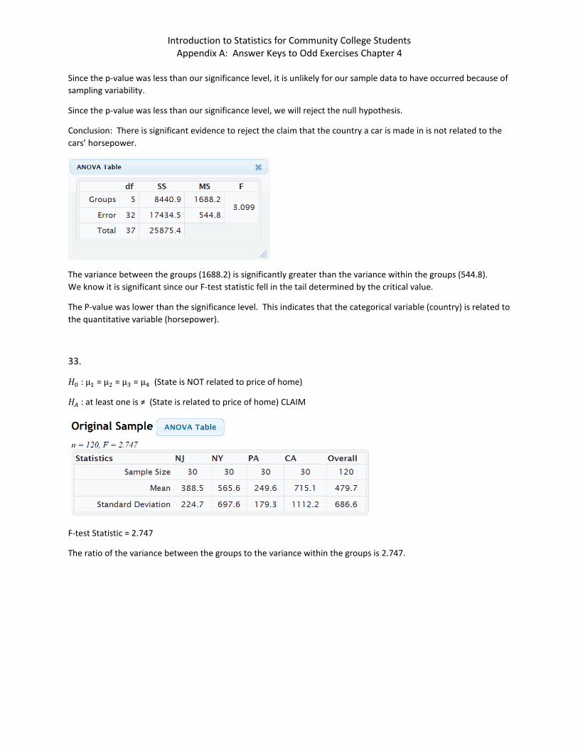
F-test Statistic = 3.099
The ratio of the variance between the groups to the variance within the groups is 3.099.

Introduction to Statistics for Community College Students Appendix A: Answer Keys to Odd Exercises Chapter 4
Critical Value Calculation
Critical Value = 1.891 (Answers were vary)
Since the test statistic 3.099 falls in the tail determined by the critical value 1.891, the sample data significantly disagrees with the null hypothesis.
P-value Calculation
P-value = 0.012 or 1.2% (Answers will vary)
Introduction to Statistics for Community College Students Appendix A: Answer Keys to Odd Exercises Chapter 4
Since the p-value was less than our significance level, it is unlikely for our sample data to have occurred because of sampling variability.
Since the p-value was less than our significance level, we will reject the null hypothesis.
Conclusion: There is significant evidence to reject the claim that the country a car is made in is not related to the cars’ horsepower.
The variance between the groups (1688.2) is significantly greater than the variance within the groups (544.8). We know it is significant since our F-test statistic fell in the tail determined by the critical value.
The P-value was lower than the significance level. This indicates that the categorical variable (country) is related to the quantitative variable (horsepower).
33.
𝐻𝐻0 : µ1 = µ2 = µ3 = µ4 (State is NOT related to price of home)
𝐻𝐻𝐴𝐴 : at least one is ≠ (State is related to price of home) CLAIM
F-test Statistic = 2.747
The ratio of the variance between the groups to the variance within the groups is 2.747.

Introduction to Statistics for Community College Students Appendix A: Answer Keys to Odd Exercises Chapter 4
Critical Value Calculation
Critical Value = 1.925 (Answers were vary)
Since the test statistic 2.747 falls in the tail determined by the critical value 1.925, the sample data significantly disagrees with the null hypothesis.
P-value Calculation
P-value = 0.023 or 2.3% (Answers will vary)

Introduction to Statistics for Community College Students Appendix A: Answer Keys to Odd Exercises Chapter 4
Since the p-value was less than our significance level, it is unlikely for our sample data to have occurred because of sampling variability.
Since the p-value was less than our significance level, we will reject the null hypothesis.
Conclusion: There is significant evidence to support the claim that the location of a home (state) is related to the price of a home.
The variance between the groups (1240611.5) is significantly greater than the variance within the groups (451576.9). We know it is significant since our F-test statistic fell in the tail determined by the critical value.
The P-value was lower than the significance level. This indicates that the categorical variable (state) is related to the quantitative variable (price).
------------------------------------------------------------------------------------------------------------------------------------------

Introduction to Statistics for Community College Students Appendix A: Answer Keys to Odd Exercises Chapter 4
Answers Problems 4C
Z-test stat
Sentence to explain Z-test statistic. Critical Value
Does the Z-test statistic fall in a tail determined by
a critical value? (Yes or No)
Does sample data
significantly disagree with
𝐻𝐻0? 1. −1.835 The sample proportion from group 1
was 1.835 standard errors below the sample proportion from group
2.
±1.645 Yes. In Tail Yes. Sig. disagree
2. +0.974 +2.576 3. −1.226 The sample proportion from group 1
was 1.226 standard errors below the sample proportion from group
2.
−1.96 No. Not in tail. No. Does not sig disagree
4. −3.177 ±1.96 5. +2.244 The sample proportion from group 1
was 2.224 standard errors above the sample proportion from group
2.
+1.645 Yes. In Tail Yes. Sig. disagree
6. +1.448 ±2.576 7. −0.883 The sample proportion from group 1
was 0.883 standard errors below the sample proportion from group
2.
−2.576 No. Not in tail. No. Does not sig disagree
8. +1.117 +1.96 9. +2.139 The sample proportion from group 1
was 2.139 standard errors above the sample proportion from group
2.
±2.576 No. Not in tail. No. Does not sig disagree
10. −0.199 −1.645

Introduction to Statistics for Community College Students Appendix A: Answer Keys to Odd Exercises Chapter 4
P-value
Proportion P-value % Sentence to explain
the P-value Significance
Level % Significance
level Proportion
If 𝐻𝐻0 is true, could the
sample data occur by random
chance or is it unlikely?
Reject 𝐻𝐻0 or Fail to reject 𝐻𝐻0?
11. 0.728 72.8% If 𝐻𝐻0 is true, there is a 72.8%
probability of getting the sample
data or more extreme because of sampling variability.
10% 0.10 Could be random chance
Fail to reject 𝐻𝐻0
12. 0.0421 1% 13. 2.11 ×
10−4 0.0211% If 𝐻𝐻0 is true, there
is a 0.0211% probability of
getting the sample data or more
extreme because of sampling variability.
5% 0.05 Unlikely to be random chance
Reject 𝐻𝐻0
14. 0.0033 1% 15. 0.176 17.6% If 𝐻𝐻0 is true, there
is a 17.6% probability of
getting the sample data or more
extreme because of sampling variability.
5% 0.05 Could be random chance
Fail to reject 𝐻𝐻0
16. 0 10% 17. 0.0628 6.28% If 𝐻𝐻0 is true, there
is a 6.28% probability of
getting the sample data or more
extreme because of sampling variability.
5% 0.05 Could be random chance
Fail to reject 𝐻𝐻0
18. 0.277 10% 19. 3.04 ×
10−6 0.000304% If 𝐻𝐻0 is true, there
is a 0.000304% probability of
getting the sample data or more
extreme because of sampling variability.
1% 0.01 Unlikely to be random chance
Reject 𝐻𝐻0
20. 0 5%

Introduction to Statistics for Community College Students Appendix A: Answer Keys to Odd Exercises Chapter 4
21. A random sample is selecting people randomly from a population. It is used to help eliminate bias and make the sample data more representative of the population. Random assignment is separating a group of people in an experiment into two or more groups randomly. This makes the groups alike, controls confounding variables and helps prove cause and effect.
23.
Two-population Proportion Assumptions (Independent groups for Experiment)
• The two categorical samples should be randomly assigned from the people or objects in the experiment. • Data values within each sample should be independent of each other. • Data values between the samples should be independent of each other. • Both samples should be at least ten successes and at least ten failures.
25.
To prove cause and effect, we would need to set up a controlled experiment. Randomly assign people in the experiment into two groups and make sure they meet the assumptions. The groups should be alike in order to control confounding variables. If the P-value is low and the groups are significantly different, this may indicate cause and effect.
27.
𝜋𝜋1: Population proportion of marijuana users that use other drugs
𝜋𝜋2: Population proportion of non-marijuana users that use other drugs
𝐻𝐻0 : 𝜋𝜋1 = 𝜋𝜋2 (Using marijuana is not related to using other drugs)
𝐻𝐻0 : 𝜋𝜋1 > 𝜋𝜋2 (Using marijuana is related to using other drugs) CLAIM
Assumptions
Random Samples? Yes both samples were collected randomly.
Individuals within and between the samples are independent? Probably yes. These were small random samples from a large population. The marijuana and non-marijuana users are unlikely to be related.
Both samples have at least 10 success and at least 10 failures? Yes. Both samples passed. Sample 1 had 87 success and 213 – 87 = 126 failures. Sample 2 had 26 success and 219 – 26 = 193 failures.
Z-test statistic = 6.850
The sample proportion for group 1 was 6.850 standard errors above the sample proportion for group 2.
The sample proportions are significantly different since the test statistic fell in the tail determined by the critical value.
P-value = 0.0000000000036839 = 0.00000000036839% ≈ 0%
If the null hypothesis is true, then there is about a 0% probability of getting the sample data or more extreme because of sampling variability.

Introduction to Statistics for Community College Students Appendix A: Answer Keys to Odd Exercises Chapter 4
The P-value is close to zero, so it is very unlikely that the sample data occurred because of sampling variability.
Since the P-value is less than the significance level, we will reject the null hypothesis.
Conclusion: There is significant evidence to support the claim that the proportion of marijuana users that use other drugs is higher than for non-marijuana users. This also indicates that using marijuana is related to using other drugs.
29.
𝜋𝜋1: Population proportion of married people that are unhappy
𝜋𝜋2: Population proportion of non-married people that are unhappy
𝐻𝐻0 : 𝜋𝜋1 = 𝜋𝜋2 (Being married is NOT related to being unhappy)
𝐻𝐻0 : 𝜋𝜋1 < 𝜋𝜋2 (Being married is related to being unhappy) CLAIM
Assumptions
Random Samples? Yes both samples were collected randomly.
Individuals within and between the samples are independent? Probably yes. These were small random samples from a large population. The married, single and divorced people are unlikely to be related.
Both samples have at least 10 success and at least 10 failures? Yes. Both samples passed. Sample 1 had 74 success and 200 – 74 = 126 failures. Sample 2 had 97 success and 200 – 97 = 103 failures.
Z-test statistic = −2.325
The sample proportion for group 1 was 2.325 standard errors below the sample proportion for group 2.
The sample proportions are significantly different since the test statistic fell in the tail determined by the critical value.
P-value = 0.0100 = 1.0%
If the null hypothesis is true, then there is about a 1.0% probability of getting the sample data or more extreme because of sampling variability.
The P-value is less than the significance level, so it is unlikely that the sample data occurred because of sampling variability.
Since the P-value is less than the significance level, we will reject the null hypothesis.
Conclusion: There is significant evidence to support the claim that married people have a lower percentage of unhappiness than non-married people. This also indicates that being married or not is related to being unhappy.

Introduction to Statistics for Community College Students Appendix A: Answer Keys to Odd Exercises Chapter 4
31.
𝜋𝜋1: Population proportion of women with a normal BMI
𝜋𝜋2: Population proportion of men with a normal BMI
𝐻𝐻0 : 𝜋𝜋1 = 𝜋𝜋2 (Gender is NOT related to having a normal BMI)
𝐻𝐻0 : 𝜋𝜋1 < 𝜋𝜋2 (Gender is related to having a normal BMI) CLAIM
The sample proportion difference is −0.106.
Tail determined by the simulation and the significance level. (Simulations and tails will vary)
Notice that the original sample difference of −0.106 does fall in the tail determined by the significance level and the simulation. This implies that the sample proportion for women was significantly lower than the sample proportion for men.
Introduction to Statistics for Community College Students Appendix A: Answer Keys to Odd Exercises Chapter 4
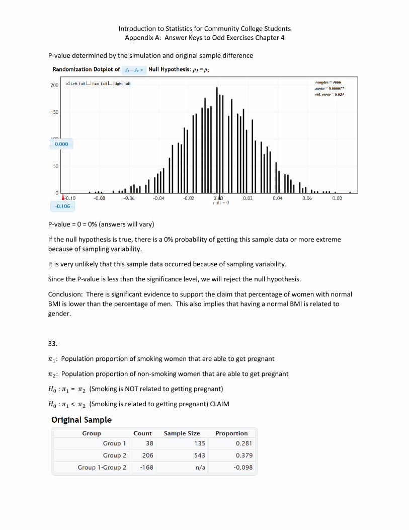
P-value determined by the simulation and original sample difference
P-value = 0 = 0% (answers will vary)
If the null hypothesis is true, there is a 0% probability of getting this sample data or more extreme because of sampling variability.
It is very unlikely that this sample data occurred because of sampling variability.
Since the P-value is less than the significance level, we will reject the null hypothesis.
Conclusion: There is significant evidence to support the claim that percentage of women with normal BMI is lower than the percentage of men. This also implies that having a normal BMI is related to gender.
33.
𝜋𝜋1: Population proportion of smoking women that are able to get pregnant
𝜋𝜋2: Population proportion of non-smoking women that are able to get pregnant
𝐻𝐻0 : 𝜋𝜋1 = 𝜋𝜋2 (Smoking is NOT related to getting pregnant)
𝐻𝐻0 : 𝜋𝜋1 < 𝜋𝜋2 (Smoking is related to getting pregnant) CLAIM

Introduction to Statistics for Community College Students Appendix A: Answer Keys to Odd Exercises Chapter 4
The sample proportion difference is −0.098.
Tail determined by the simulation and the significance level. (Simulations and tails will vary)
Notice that the original sample difference of −0.098 does fall in the tail determined by the significance level and the simulation. This implies that the sample proportion for smokers was significantly lower than the sample proportion for non-smokers.
P-value determined by the simulation and original sample difference
P-value = 0.013 = 1.3% (answers will vary)
If the null hypothesis is true, there is a 1.3% probability of getting this sample data or more extreme because of sampling variability.

Introduction to Statistics for Community College Students Appendix A: Answer Keys to Odd Exercises Chapter 4
It is very unlikely that this sample data occurred because of sampling variability.
Since the P-value is less than the significance level, we will reject the null hypothesis.
Conclusion: There is significant evidence to support the claim that percentage of smokers that are able to get pregnant is lower than the percentage of non-smokers. This also implies that getting pregnant is related to smoking or not.
------------------------------------------------------------------------------------------------------------------------------------------
Answers Problems 4D
𝜒𝜒2-test stat
Sentence to explain 𝜒𝜒2-test statistic. Critical Value
Does the 𝜒𝜒2-test statistic fall in a tail determined by the
critical value? (Yes or No)
Does sample data
significantly disagree with
𝐻𝐻0? 1. +28.573 The sum of the averages of the
squares of the differences between the observed sample values and the
expected values from the null hypothesis is 28.573.
+9.117 Yes. In tail. Yes. Significantly disagrees.
2. +1.226 +7.113 3. +2.137 The sum of the averages of the
squares of the differences between the observed sample values and the
expected values from the null hypothesis is 2.137
+5.521 No. Not in tail. No. Does not significantly
disagree.
4. +14.415 +6.114 5. +3.718 The sum of the averages of the
squares of the differences between the observed sample values and the
expected values from the null hypothesis is 3.718
+7.182 No. Not in tail. No. Does not significantly
disagree.
6. +0.891 +3.994 7. +51.652 The sum of the averages of the
squares of the differences between the observed sample values and the
expected values from the null hypothesis is 51.652
+14.881 Yes. In tail. Yes. Significantly disagrees.
8. +1.185 +4.181 9. +2.442 The sum of the averages of the
squares of the differences between the observed sample values and the
expected values from the null hypothesis is 2.442
+8.619 No. Not in tail. No. Does not significantly
disagree.
10. +14.133 +10.336

Introduction to Statistics for Community College Students Appendix A: Answer Keys to Odd Exercises Chapter 4
P-value Proportion
P-value % Sentence to explain the P-
value
Significance Level %
Significance level
Proportion
If 𝐻𝐻0 is true, could the
sample data occur by random
chance or is it unlikely?
Reject 𝐻𝐻0 or Fail to reject 𝐻𝐻0?
11. 0.0006 0.06% If 𝐻𝐻0 is true, there is a 0.06%
probability of getting the sample
data or more extreme by
sampling variability.
10% 0.1 Unlikely Reject 𝐻𝐻0
12. 0.042 1% 13. 9.16 × 10⁻⁷ 0.0000916% If 𝐻𝐻0 is true, there
is a 0.0000916% probability of
getting the sample data or more extreme by
sampling variability.
5% 0.05 Unlikely Reject 𝐻𝐻0
14. 0.739 1% 15. 0.0035 0.35% If 𝐻𝐻0 is true, there
is a 0.35% probability of
getting the sample data or more extreme by
sampling variability.
5% 0.05 Unlikely Reject 𝐻𝐻0
16. 0 10% 17. 0.419 41.9% If 𝐻𝐻0 is true, there
is a 41.9% probability of
getting the sample data or more extreme by
sampling variability.
5% 0.05 Could be Fail to reject 𝐻𝐻0
18. 0.0274 10% 19. 3.77 × 10⁻⁵ 0.00377% If 𝐻𝐻0 is true, there
is a 0.00377% probability of
getting the sample data or more extreme by
1% 0.01 Unlikely Reject 𝐻𝐻0

Introduction to Statistics for Community College Students Appendix A: Answer Keys to Odd Exercises Chapter 4
sampling
variability. 20. 0.067 5%
21.
Goodness of Fit Degrees of Freedom = K – 1
(K is the number of groups)
23.
For each group, the computer subtracts the expected count (Ho) from the observed count (Sample). It then squares the differences to get rid of negatives. It then divides each square by the expected count. Lastly, it adds up this calculation for each group to get the total chi-squared.
25.
If the observed sample counts and the expected counts from the Ho were close, the differences would be very small. That would cause the overall chi-squared to be small.
27.
𝐻𝐻0 : 𝜋𝜋𝑏𝑏𝑏𝑏𝑏𝑏𝑏𝑏 = 0.01, 𝜋𝜋𝑐𝑐𝑐𝑐𝑐𝑐𝑐𝑐𝑐𝑐𝑐𝑐𝑐𝑐 = 0.1, 𝜋𝜋𝑑𝑑𝑐𝑐𝑏𝑏𝑑𝑑𝑏𝑏 𝑐𝑐𝑐𝑐𝑐𝑐𝑎𝑎𝑏𝑏 = 0.8, 𝜋𝜋𝑑𝑑𝑐𝑐𝑐𝑐𝑐𝑐𝑐𝑐𝑏𝑏𝑑𝑑 𝑐𝑐𝑜𝑜𝑜𝑜 = 0.05, 𝜋𝜋𝑐𝑐𝑝𝑝𝑏𝑏𝑐𝑐𝑏𝑏𝑐𝑐 𝑡𝑡𝑐𝑐𝑐𝑐𝑎𝑎𝑡𝑡𝑐𝑐 = 0.02, 𝜋𝜋𝑤𝑤𝑐𝑐𝑐𝑐𝑏𝑏 = 0.02
𝐻𝐻𝐴𝐴 : At least one proportion is ≠ (CLAIM)
Degrees of freedom = 6 – 1 = 5
Chi-squared test stat = 3.816
The sum of the averages of the squares of the differences between the observed sample counts and the expected counts from the null hypothesis is 3.816.

Introduction to Statistics for Community College Students Appendix A: Answer Keys to Odd Exercises Chapter 4
Critical value and Tail calculation from simulation and significance level (answers will vary)
Critical Value = 11.523 (answers will vary)
The test statistic of 3.816 does not fall in the tail determined by the critical value. So the sample data does not significantly disagree with the null hypothesis. Also the observed sample counts are not significantly different than the expected counts from the null hypothesis.
P-value calculation from the test statistic and simulation (answers will vary)

Introduction to Statistics for Community College Students Appendix A: Answer Keys to Odd Exercises Chapter 4
P-value = 0.575 = 57.5% (answers will vary)
If the null hypothesis was true, then there is a 57.5% probability of getting the sample data or more extreme by sampling variability.
The P-value is much higher than the 5% significance level. So this sample data could have occurred simply by sampling variability.
Fail to reject the null hypothesis.
Conclusion: There is not significant evidence to support the claim that the percentages listed by the employee are wrong. They might be correct, but we do not have evidence.
This problem is the second type of goodness of fit test and is not designed to explore relationships. The P-value in this case was trying to test the accuracy of the given percentages, not tell if the variables are related. The percentages being so vastly different does indicate that type of transportation is probably related to the percentage of people that use that type.
29.
𝐻𝐻0 : 𝜋𝜋𝑐𝑐𝑐𝑐𝑝𝑝𝑐𝑐𝑐𝑐𝑡𝑡𝑏𝑏𝑐𝑐𝑎𝑎 = 0.54, 𝜋𝜋𝑐𝑐𝑜𝑜𝑐𝑐𝑏𝑏𝑐𝑐𝑐𝑐𝑎𝑎 𝑐𝑐𝑎𝑎𝑏𝑏𝑐𝑐𝑏𝑏𝑐𝑐𝑐𝑐𝑎𝑎 = 0.18, 𝜋𝜋ℎ𝑏𝑏𝑡𝑡𝑐𝑐𝑐𝑐𝑎𝑎𝑏𝑏𝑐𝑐 𝑐𝑐𝑎𝑎𝑏𝑏𝑐𝑐𝑏𝑏𝑐𝑐𝑐𝑐𝑎𝑎 = 0.12, 𝜋𝜋𝑐𝑐𝑡𝑡𝑏𝑏𝑐𝑐𝑎𝑎 𝑐𝑐𝑎𝑎𝑏𝑏𝑐𝑐𝑏𝑏𝑐𝑐𝑐𝑐𝑎𝑎 = 0.15, 𝜋𝜋𝑐𝑐𝑡𝑡ℎ𝑏𝑏𝑐𝑐 = 0.01
𝐻𝐻𝐴𝐴 : At least one proportion is ≠ (CLAIM)
Degrees of freedom = 5 – 1 = 4
Chi-squared test stat = 357.362
The sum of the averages of the squares of the differences between the observed sample counts and the expected counts from the null hypothesis is 357.362.

Introduction to Statistics for Community College Students Appendix A: Answer Keys to Odd Exercises Chapter 4
Critical value and Tail calculation from simulation and significance level (answers will vary)
Critical Value = 13.831 (answers will vary)
The test statistic of 357.362 is way out in the far tail determined by the critical value. So the sample data significantly disagrees with the null hypothesis. Also the observed sample counts are significantly different than the expected counts from the null hypothesis.
P-value calculation from the test statistic and simulation (answers will vary)

Introduction to Statistics for Community College Students Appendix A: Answer Keys to Odd Exercises Chapter 4
P-value = 0 = 0% (answers may vary)
If the null hypothesis was true, then there is a 0% probability of getting the sample data or more extreme by sampling variability.
The P-value is much lower than the 1% significance level. It is highly unlikely for this sample data to have occurred simply by sampling variability.
Reject the null hypothesis.
Conclusion: There is significant evidence to support the claim that the juries from this county are not representing the demographic.
This problem is the second type of goodness of fit test and is not designed to explore relationships. The P-value in this case was trying to test the accuracy of the given percentages, not tell if the variables are related. The percentages being so vastly different does indicate that race is most likely related to the percentages.
31.
29.
𝐻𝐻0 : 𝜋𝜋𝑎𝑎𝑐𝑐𝑎𝑎𝑑𝑑𝑐𝑐𝑚𝑚 = 𝜋𝜋𝑡𝑡𝑝𝑝𝑏𝑏𝑡𝑡𝑑𝑑𝑐𝑐𝑚𝑚 = 𝜋𝜋𝑤𝑤𝑏𝑏𝑑𝑑𝑎𝑎𝑏𝑏𝑡𝑡𝑑𝑑𝑐𝑐𝑚𝑚 = 𝜋𝜋𝑡𝑡ℎ𝑝𝑝𝑐𝑐𝑡𝑡𝑑𝑑𝑐𝑐𝑚𝑚 = 𝜋𝜋𝑜𝑜𝑐𝑐𝑏𝑏𝑑𝑑𝑐𝑐𝑚𝑚 = = 𝜋𝜋𝑡𝑡𝑐𝑐𝑡𝑡𝑝𝑝𝑐𝑐𝑑𝑑𝑐𝑐𝑚𝑚 = 𝜋𝜋𝑡𝑡𝑝𝑝𝑎𝑎𝑑𝑑𝑐𝑐𝑚𝑚
𝐻𝐻𝐴𝐴 : At least one proportion is ≠ (CLAIM)
Degrees of freedom = 7 – 1 = 6
Chi-squared test stat = 7.5478
The sum of the averages of the squares of the differences between the observed sample counts and the expected counts from the null hypothesis is 7.5478.
Critical Value = 16.8119
The test statistic of 7.5478 does not fall in the tail determined by the critical value. So the sample data does NOT significantly disagrees with the null hypothesis. Also the observed sample counts are NOT significantly different than the expected counts from the null hypothesis.
P-value = 0.2731 = 27.31% (answers may vary)
If the null hypothesis was true, then there is a 27.31% probability of getting the sample data or more extreme by sampling variability.
The P-value is higher than the 1% significance level. This sample data could have occurred simply by sampling variability.
Fail to reject the null hypothesis.

Introduction to Statistics for Community College Students Appendix A: Answer Keys to Odd Exercises Chapter 4
Conclusion: There is not significant evidence to support the claim that the probability of having a fatal car accident is different on the various days of the week. This also implies that the day of the week is probably not related to having a fatal car accident.
------------------------------------------------------------------------------------------------------------------------------------------
Answers Problems 4E
1. If conditional proportions are significantly different from one group to another, it indicates that the categorical variable that decides the groups is probably related to the categorical variable that the proportions came from.
#3-9
3. At the end of yes smoking row in the overall chart we see the answer is 0.089 or 8.9%.
5. In the overall chart where no smoking and carpool meet, we see the answer is 0.086 or 8.6%.
7. We will use the union “or” formula. These individual proportions we can get from the overall chart.
P ( no smoke OR dropped off) = P(no smoke) + P(dropped off) – P(no smoke and dropped off) = 0.911 + 0.055 – 0.052 = 0.914 or 91.4%

Introduction to Statistics for Community College Students Appendix A: Answer Keys to Odd Exercises Chapter 4
9. Since the conditions are smoking and not smoking and they are a row, we will use the row chart for conditional %.
P(carpool given smoke) = 0.069 = 6.9%
P(carpool given not smoke) = 0.094 = 9.4%
These appear significantly different. (36% increase) So smoking or not does appear to be related to carpooling.
#11-18
Rows: text and drive or not
Columns: car accident or not

Introduction to Statistics for Community College Students Appendix A: Answer Keys to Odd Exercises Chapter 4
11. At the end of yes texting and driving row in the overall chart we see the answer is 0.399 or 39.9%.
13. In the overall chart where yes text and drive and yes car accident meet, we see the answer is 0.13 or 13%.
15. We will use the union “or” formula. These individual proportions we can get from the overall chart.
P ( yes text drive OR no car accident) = P(yes text drive) + P(no car accident) – P(yes text drive AND no car accident) = 0.399 + 0.749 – 0.269 = 0.879 or 87.9%
17. Since the conditions are text & drive and not text & drive are a row, we will use the row chart.
P(car accident given text&drive) = 0.326 = 32.6%
P(car accident given not text&drive) = 0.201 = 20.1%

Introduction to Statistics for Community College Students Appendix A: Answer Keys to Odd Exercises Chapter 4
These appear significantly different. (62.2% increase) So car accidents do appear to be related to texting an driving or not.
#19-26
19. At the end of yes tattoo row in the overall chart we see the answer is 0.261 or 26.1%.
21. In the overall chart where Facebook and no tattoo meet, we see the answer is 0.172 or 17.2%.
23. We will use the union “or” formula. These individual proportions we can get from the overall chart.
P ( yes tattoo OR Instagram) = P(yes tattoo) + P(Instagram) – P(yes tattoo AND Instagram) =
= 0.261 + 0.38 – 0.126 = 0.515 or 51.5%

Introduction to Statistics for Community College Students Appendix A: Answer Keys to Odd Exercises Chapter 4
25. Since the conditions of tattoo and no tattoo are in a row, we will use the row chart for conditional %.
P(Twitter given tattoo) = 0.094 = 9.4%
P(Twitter given no tattoo) = 0.087 = 8.7%
These appear to be relatively close. (Only 8% increase) So having a tattoo or not does not appear to be related to liking Twitter.
#27-34
27. At the end of the Germany column in the overall chart we see the answer is 0.132 or 13.2%.
29. In the overall chart where Japan and four cylinders meet, we see the answer is 0.158 or 15.8%.

Introduction to Statistics for Community College Students Appendix A: Answer Keys to Odd Exercises Chapter 4
31. We will use the union “or” formula. These individual proportions we can get from the overall chart.
P ( Germany OR Six Cylinders) = P(Germany) + P(Six Cylinders) – P(Germany AND Six Cylinders) =
= 0.132 + 0.263 – 0 = 0.395 or 39.5%
33. Since the conditions of Japan and Germany are in a column, we will use the column chart for conditional %.
P(Four Cylinders given Japan) = 0.857 = 85.7%
P(Four Cylinders given Germany) = 0.8 = 80%
These appear to be relatively close. (Only 7.1% increase) So the country (Japan and Germany) is probably not related to having four cylinders.
------------------------------------------------------------------------------------------------------------------------------------------

Introduction to Statistics for Community College Students Appendix A: Answer Keys to Odd Exercises Chapter 4
Answers Problems 4F
𝜒𝜒2-test stat
Sentence to explain 𝜒𝜒2-test statistic. Critical Value
Does the 𝜒𝜒2-test statistic fall in a tail determined by the
critical value? (Yes or No)
Does sample data
significantly disagree with
𝐻𝐻0? 1. +1.573 The sum of the averages of the
squares of the differences between the observed sample values and the
expected values from the null hypothesis is 1.573.
+4.117 No. Not in tail. No. Does not significantly
disagree.
2. +6.226 +5.118 3. +2.144 The sum of the averages of the
squares of the differences between the observed sample values and the
expected values from the null hypothesis is 2.144.
+4.121 No. Not in tail. No. Does not significantly
disagree.
4. +3.415 +5.091 5. +13.718 The sum of the averages of the
squares of the differences between the observed sample values and the
expected values from the null hypothesis is 13.718.
+7.189 Yes. In tail. Yes. Significantly disagrees.
6. +0.972 +4.812 7. +31.652 The sum of the averages of the
squares of the differences between the observed sample values and the
expected values from the null hypothesis is 31.652.
+12.557 Yes. In tail. Yes. Significantly disagrees.
8. +11.185 +5.181 9. +25.443 The sum of the averages of the
squares of the differences between the observed sample values and the
expected values from the null hypothesis is 25.443.
+7.008 Yes. In tail. Yes. Significantly disagrees.
10. +1.133 +8.336

Introduction to Statistics for Community College Students Appendix A: Answer Keys to Odd Exercises Chapter 4
P-value
Proportion P-value % Sentence to
explain the P-value
Significance Level %
Significance level
Proportion
If 𝐻𝐻0 is true, could the
sample data occur by random
chance or is it unlikely?
Reject 𝐻𝐻0 or Fail to reject 𝐻𝐻0?
11. 0.263 26.3% If 𝐻𝐻0 is true, there is a 26.3%
probability of getting the sample
data or more extreme by
sampling variability
10% 0.1 Could be Fail to reject 𝐻𝐻0
12. 0.0042 1% 13. 5.22 × 10⁻⁴ 0.0522% If 𝐻𝐻0 is true, there
is a 0.0522% probability of
getting the sample data or more extreme by
sampling variability
5% 0.05 Unlikely Reject 𝐻𝐻0
14. 0.0639 1% 15. 0 0% If 𝐻𝐻0 is true, there
is a 0% probability of getting the
sample data or more extreme by
sampling variability
5% 0.05 Unlikely Reject 𝐻𝐻0
16. 0.539 10% 17. 0.0419 4.19% If 𝐻𝐻0 is true, there
is a 4.19% probability of
getting the sample data or more extreme by
sampling variability
5% 0.05 Unlikely Reject 𝐻𝐻0
18. 0.0027 10% 19. 7.73 × 10⁻⁸ 0.00000773% If 𝐻𝐻0 is true, there
is a 0.00000773% probability of
getting the sample data or more extreme by
sampling variability
1% 0.01 Unlikely Reject 𝐻𝐻0
20. 0.674 5%

Introduction to Statistics for Community College Students Appendix A: Answer Keys to Odd Exercises Chapter 4
21.
To perform a categorical association test in Statcato, follow the following steps.
If you have a contingency table, then type the contingency table in data sheet. Column titles will be in the gray where it says VAR. Click on the “statistics” menu and then click “multinomial experiments”. Then click on “chi-square contingency table”. Click on the columns that contain your counts in your contingency table and press “add to list”. Then put in the significance level and press “OK”.
If you have two raw categorical data sets, copy and paste them into the data sheet. Titles should be in the gray where it says VAR. Click on the “statistics” menu and then click “Cross Tabulation and Chi-square”. Click on the row and column, the significance level and then press “OK”.
23.
Categorical Association Test Assumptions (one random sample)
• The categorical sample or samples should be collected randomly or be representative of the population. • Data values within each sample should be independent of each other. • The expected counts from the null hypothesis should be at least five.
25.
Expected Counts = (𝑅𝑅𝑐𝑐𝑤𝑤 𝑇𝑇𝑐𝑐𝑡𝑡𝑐𝑐𝑐𝑐 𝑥𝑥 𝐶𝐶𝑐𝑐𝑐𝑐𝑝𝑝𝑎𝑎𝑎𝑎 𝑇𝑇𝑐𝑐𝑡𝑡𝑐𝑐𝑐𝑐)𝐺𝐺𝑐𝑐𝑐𝑐𝑎𝑎𝑑𝑑 𝑇𝑇𝑐𝑐𝑡𝑡𝑐𝑐𝑐𝑐
27.
If the expected counts from the null hypothesis are close to the observed sample counts, then the differences between them will be close to zero. This will make the chi-squared test statistic very small and not fall in the tail. This would indicate that the sample data (observed counts) does not significantly disagree with the null hypothesis (expected counts).
29.
𝐻𝐻0 : Blood type is not related to the Rh
𝐻𝐻𝐴𝐴 : Blood type is related to the Rh (CLAIM)
Assumptions
Random? Yes. Given
Individuals Independent? Probably. Since this was a small random sample from a very large population.
Expected Counts at least 5? No. (The expected counts were 36.03, 23.0, 16.1, 85.87, 10.97, 7.0, 4.9, and 26.13)
Notice one of the expected counts (4.9) was below 5.
𝜒𝜒2 Test Statistic = 8.5522
The sum of the averages of the squares of the differences between the observed sample counts and the expected counts from the null hypothesis is 8.5522.

Introduction to Statistics for Community College Students Appendix A: Answer Keys to Odd Exercises Chapter 4
The sample data significantly disagrees with the null hypothesis since the test statistic falls in the right tail determined by the critical value 6.2514. This also indicates that the observed sample counts were significantly different than the expected counts.
P-value = 0.0359 = 3.59%
If the null hypothesis is true, there is a 3.59% probability of getting the sample data or more extreme by sampling variability.
The P-value is lower than the 10% significance level.
It is unlikely for this data to have occurred by sampling variability.
Reject 𝐻𝐻0.
If the sample data had met the assumptions, then the conclusion would be: There is significant evidence to support the claim that a persons’ blood type is related to the Rh. However, this data did not meet all of the assumptions, so evidence is in question.
The P-value is low, indicating that blood type and Rh are likely to be related. However, our data did not meet all of the assumptions, so our evidence for this is in question.
31.
𝐻𝐻0 : Health is not related to education
𝐻𝐻𝐴𝐴 : Health is related to education (CLAIM)
Assumptions
Random? Yes. Given
Individuals Independent? Probably. Since this was a small random sample from a very large population.
Expected Counts at least 5? Yes. (The expected counts were 148.64, 249.76, 106.91, 29.70, 502.31, 844.04, 361.29, 100.36, 77.24, 129.78, 55.55, 15.43, 161.42, 271.23, 116.10, 32.25, 86.40, 145.19, 62.15, and 17.26) All were greater than 5.
𝜒𝜒2 Test Statistic = 285.0610
The sum of the averages of the squares of the differences between the observed sample counts and the expected counts from the null hypothesis is 285.0610.
The sample data significantly disagrees with the null hypothesis since the test statistic falls in the right tail determined by the critical value 21.0261. This also indicates that the observed sample counts were significantly different than the expected counts.
P-value = 0 = 0%
If the null hypothesis is true, there is a 0% probability of getting the sample data or more extreme by sampling variability.
The P-value is lower than the 5% significance level.
It is unlikely for this data to have occurred by sampling variability.

Introduction to Statistics for Community College Students Appendix A: Answer Keys to Odd Exercises Chapter 4
Reject 𝐻𝐻0.
Conclusion: There is significant evidence to support the claim that a persons’ health is related to their education.
The P-value is low, indicating that health and education are likely to be related.
33.
𝐻𝐻0 : The country a car is made in is not related to the number of cylinders.
𝐻𝐻𝐴𝐴 : The country a car is made in is related to the number of cylinders. (CLAIM)
Assumptions
Random? Yes. The car data was collected randomly.
Individuals Independent? Probably not. The population of types of cars is not that large and many types of cars are owned by the same company. The company may have similar numbers of cylinders in their cars.
Expected Counts at least 5? No. Most of the expected counts were below 5. This means this data would not be suitable for using the traditional chi-squared distribution. Notice the simulation does not look like it fits the chi-squared distribution very well. However this data may be used for simulation if the independence assumption and random had passed.

Introduction to Statistics for Community College Students Appendix A: Answer Keys to Odd Exercises Chapter 4
Degrees of freedom = (r – 1)(c – 1) = (6 – 1)(4 – 1) = (5)(3) = 15
𝜒𝜒2 Test Statistic = 22.267
The sum of the averages of the squares of the differences between the observed sample counts and the expected counts from the null hypothesis is 22.267.
Critical Value and tail Calculation determined by significance level (simulations will vary)
Approximate Critical value = 49.535 (answers may vary)
Notice that the Chi-square test statistic does not fall in the tail determined by the critical value. So the sample data does not significantly disagree with the null hypothesis. This also indicates that the observed sample counts were not significantly different than the expected counts.

Introduction to Statistics for Community College Students Appendix A: Answer Keys to Odd Exercises Chapter 4
P-value calculation with test statistic (P-values will vary)
Approximate P-value = 0.127 = 12.7% (answers will vary)
If the null hypothesis is true, there is a 12.7% probability of getting the sample data or more extreme by sampling variability.
The P-value is higher than the 1% significance level.
This sample data could have occurred by sampling variability.
Fail to reject 𝐻𝐻0.
Conclusion: There is NOT significant evidence to support the claim that the country a car is made in is related to the number of cylinders.
The P-value is high, indicating that the country and cylinders are likely to be not related. However, a high P-value is not evidence and this data did not pass all of the assumptions for randomized simulation.

Introduction to Statistics for Community College Students Appendix A: Answer Keys to Odd Exercises Chapter 4
35.
𝐻𝐻0 : Tattoos are not related to social media. (CLAIM)
𝐻𝐻𝐴𝐴 : Tattoos are related to social media.
Assumptions
Random or representative? Yes. This data was a census of all math 140 students during the fall 2015 semester. Though it is not random, it is likely to be representative of all math 140 students in all semester.
Individuals Independent? No. The individual students came from the same classes.
Expected Counts at least 5? Yes. All of the expected counts were greater than 5.
Degrees of freedom = (r – 1)(c – 1) = (5 – 1)(2 – 1) = (4)(1) = 4
𝜒𝜒2 Test Statistic = 7.531
The sum of the averages of the squares of the differences between the observed sample counts and the expected counts from the null hypothesis is 7.531.

Introduction to Statistics for Community College Students Appendix A: Answer Keys to Odd Exercises Chapter 4
Critical Value and tail Calculation determined by significance level (simulations will vary)
Approximate Critical value = 9.132 (answers may vary)
Notice that the Chi-square test statistic does not fall in the tail determined by the critical value. So the sample data does not significantly disagree with the null hypothesis. This also indicates that the observed sample counts were not significantly different than the expected counts.

Introduction to Statistics for Community College Students Appendix A: Answer Keys to Odd Exercises Chapter 4
P-value calculation with test statistic (P-values will vary)
Approximate P-value = 0.105 = 10.5% (answers will vary)
If the null hypothesis is true, there is a 10.5% probability of getting the sample data or more extreme by sampling variability.
The P-value is higher than the 5% significance level.
This sample data could have occurred by sampling variability.
Fail to reject 𝐻𝐻0.
Conclusion: There is NOT significant evidence to reject the claim that tattoos are not related to social media.
The P-value is high, indicating that tattoos are likely to be not related. However, the high P-value is not evidence and this data did not pass all of the assumptions for randomized simulation.
--------------------------------------------------------------------------------------------------------------------------------------------------------

Introduction to Statistics for Community College Students Appendix A: Answer Keys to Odd Exercises Chapter 4
Answers Problems 4G
1. The response variable (Y) is the focus of the correlation study and the variable you want to make predictions about.
3. R-squared is the percentage of variability in the response variable (Y) that can be explained by the explanatory variable (X).
5. The slope of the regression line is the amount of increase or decrease in the response variable (Y) for every 1 unit increase in the explanatory variable (x).
7. Regression line formulas are only accurate in the scope of the X-values. Extrapolation is making a prediction outside the scope of the X-value. So when a person extrapolates, they plug in a number into the formula that the formula was never designed for. Extrapolation results in predictions that are not accurate and have a lot of error.
9.
a.
The scatterplot and the correlation coefficient indicate a strong positive correlation between nicotine and carbon monoxide.
b.
𝑟𝑟2 = 0.8632 ≈ 0.745 = 74.5%
74.5% of the variability in carbon monoxide can be explained by the linear relationship with nicotine.
c.
Slope = +12.306
For every one mg increase in nicotine, the average carbon monoxide is increasing 12.306 ppm.
d.
Y-intercept = 0.795

Introduction to Statistics for Community College Students Appendix A: Answer Keys to Odd Exercises Chapter 4
If a cigarette has zero mg of nicotine, then the predicted amount of carbon monoxide would be 0.795 ppm.
Yes. The Y-intercept sentence seems to make sense. The Y-intercept is probably not very accurate since zero is not in the scope of the x values. Hence plugging in zero would be an extrapolation.
e.
The points in the scatterplot are 2.3 ppm from the regression line on average.
The average prediction error is 2.3 ppm.
f.
Regression Line: Y = 0.795 + 12.306 X
Prediction of Y (ppm) when X = 1.2 mg nicotine
Y = 0.795 + 12.306 X
Y = 0.795 + 12.306 (1.2)
Y = 0.795 + 14.7672
Y = 15.5622 ppm
If a cigarette has 1.2 mg of nicotine, we predict the carbon monoxide to be 15.5622 ppm.
(This prediction could be off by 2.3 ppm on average.)
11.
a.
The scatterplot and the correlation coefficient indicate a strong positive correlation between nicotine and carbon monoxide.

Introduction to Statistics for Community College Students Appendix A: Answer Keys to Odd Exercises Chapter 4
b.
𝑟𝑟2 = 0.9082 ≈ 0.824 = 82.4%
82.4% of the variability in weight can be explained by the linear relationship with waist size.
c.
Slope = +2.395
For every one cm increase in waist size, the average weight of the adults is increasing 2.395 pounds.
d.
Y-intercept = -51.728
If the waist size was zero cm, then the predicted weight would be -51.728 pounds.
No the Y-intercept does not make sense. It is impossible for the waist size of an adult to be zero cm. It is also impossible for the weight of an adult to be -51.728 pounds. The Y-intercept is not accurate since zero is not in the scope of the x values. Hence plugging in zero would be an extrapolation.
e.
The points in the scatterplot are 14.6809 pounds from the regression line on average.
The average prediction error is 14.6809 pounds.
f.
Regression Line: Y = -51.728 + 2.395 X
Prediction of Y (pounds) when X = 100 cm (waist)
Y = -51.728 + 2.395 X
Y = -51.728 + 2.395 (100)
Y = -51.728 + 239.5
Y = 187.772 pounds
If an adults waist size is 100 cm, we predict the weight to be 187.772 pounds.
(This prediction could be off by 14.608 pounds on average.)

Introduction to Statistics for Community College Students Appendix A: Answer Keys to Odd Exercises Chapter 4
13.
a.
The scatterplot and the correlation coefficient indicate a strong positive correlation between the age and length of bears.
b.
𝑟𝑟2 = 0.7192 ≈ 0.517 = 51.7%
51.7% of the variability in bear length can be explained by the linear relationship with the age of the bear.
c.
Slope = +0.228
For every one month older a bear gets, the average length of the bears is increasing 0.228 inch.
d.
Y-intercept = 48.69
If the age of the bear is zero months old, then the predicted length would be 48.69 inches.
The Y-intercept does make sense as the average length of a newborn bear. The Y-intercept is not accurate though since zero is not in the scope of the x values. Hence plugging in zero would be an extrapolation. It is no surprise that the predicted length is way off from what we expect in a newborn bear.
e.
The points in the scatterplot are 7.51 inches from the regression line on average.
The average prediction error is 7.51 inches.
f.

Introduction to Statistics for Community College Students Appendix A: Answer Keys to Odd Exercises Chapter 4
Regression Line: Y = 48.69 + 0.228 X
Prediction of Y (length in inches) when X = 24 months (age)
Y = 48.69 + 0.228 X
Y = 48.69 + 0.228 (24)
Y = 48.69 + 5.472
Y = 54.162 inches
If a bear is 24 months old, we predict the length to be 54.162 inches.
(This prediction could be off by 7.51 inches on average.)
15.
a.
The scatterplot and the correlation coefficient indicate a strong negative correlation between the weight of a car and the gas mileage.
b.
𝑟𝑟2 = (−0.903)2 ≈ 0.815 = 81.5%
81.5% of the variability in gas mileage can be explained by the linear relationship with the weight of the car.
c.
Slope = −8.372
For every 1 ton increase in the weight of a car, the average gas mileage decreases 8.372 mpg.
d.

Introduction to Statistics for Community College Students Appendix A: Answer Keys to Odd Exercises Chapter 4
Y-intercept = 48.741
If the weight of a car is zero tons, then the predicted gas mileage would be 48.741 mpg.
The Y-intercept does not make sense. It is impossible for the weight of a car to be zero tons. The Y-intercept is not accurate though since zero is not in the scope of the x values. Hence plugging in zero would be an extrapolation.
e.
The points in the scatterplot are 2.8516 mpg from the regression line on average.
The average prediction error is 2.8516 mpg.
f.
Regression Line: Y = 48.741 − 8.372 X
Prediction of Y (mpg) of car when weight X = 3 tons
Y = 48.741 − 8.372 X
Y = 48.741 − 8.372 (3)
Y = 48.741 – 25.116
Y = 23.625 mpg
If a car weighs 3 tons, we predict the average gas mileage to be 23.625 mpg.
(This prediction could be off by 2.8516 mpg on average.)
-----------------------------------------------------------------------------------------------------------------------------------------

Introduction to Statistics for Community College Students Appendix A: Answer Keys to Odd Exercises Chapter 4
Problems 4H Answers
T-test statistic or Correlation Coefficient (r)
Sentence to explain T-test statistic or
Correlation Coefficient (r)
Critical Value
(T or r)
Does the T-test statistic or r-value fall in a tail
determined by a critical value?
(Yes or No)
Does sample data significantly
disagree with 𝐻𝐻0?
1. T = −2.441 The slope is 2.441 standard errors below
zero.
±1.775 Yes. In tail. Significantly Disagrees with 𝐻𝐻0
2. r = 0.183 0.316 3. T = +1.166 The slope is 1.166
standard errors above zero.
+2.003 No. Not in tail. Does NOT significantly
Disagrees with 𝐻𝐻0 4. r = −0.799 ±0.286 5. T = +3.118 The slope is 3.118
standard errors above zero.
+2.714 Yes. In tail. Significantly Disagrees with 𝐻𝐻0
6. r = 0.921 0.339 7. T = −0.852 The slope is 0.852
standard errors below zero.
±2.322 No. Not in tail. Does NOT significantly
Disagrees with 𝐻𝐻0 8. r = −0.026 −0.279 9. T = +1.339 The slope is 1.339
standard errors above zero.
±1.997 No. Not in tail. Does NOT significantly
Disagrees with 𝐻𝐻0 10. r = 0.483 +0.303

Introduction to Statistics for Community College Students Appendix A: Answer Keys to Odd Exercises Chapter 4
P-value
Proportion P-value % Sentence to
explain the P-value Significance
Level % Significance
level Proportion
If 𝐻𝐻0 is true, could the
sample data occur by random
chance or is it unlikely?
Reject 𝐻𝐻0 or Fail to reject 𝐻𝐻0?
11. 0.521 52.1% If 𝐻𝐻0 is true, there is a 52.1%
probability of getting the sample
data or more extreme by
sampling variability.
10% 0.10 Could be sampling variability (random chance)
Fail to reject 𝐻𝐻0
12. 0.0426 1% 13. 3.41 ×
10−5 0.00341% If 𝐻𝐻0 is true, there
is a 0.00341% probability of
getting the sample data or more extreme by
sampling variability.
5% 0.05 Unlikely to be sampling variability (random chance)
Reject 𝐻𝐻0
14. 0.0033 1% 15. 0.768 76.8% If 𝐻𝐻0 is true, there
is a 76.8% probability of
getting the sample data or more extreme by
sampling variability.
5% 0.05 Could be sampling variability (random chance)
Fail to reject 𝐻𝐻0
16. 0 10% 17. 0.0428 4.28% If 𝐻𝐻0 is true, there
is a 4.28% probability of
getting the sample data or more extreme by
sampling variability.
5% 0.05 Unlikely to be sampling variability (random chance)
Reject 𝐻𝐻0
18. 0.277 10% 19. 6.04 ×
10−6 0.000604% If 𝐻𝐻0 is true, there
is a 0.000604% probability of
getting the sample data or more extreme by
sampling variability.
1% 0.01 Unlikely to be sampling variability (random chance)
Reject 𝐻𝐻0
20. 0.0178 5%

Introduction to Statistics for Community College Students Appendix A: Answer Keys to Odd Exercises Chapter 4
21.
Correlation Test Assumptions: Quantitative ordered pair sample data collected randomly, Data values within the sample should be independent of each other, the sample size should be at least 30, the scatterplot and correlation coefficient (r) should show some linear pattern, there should be no influential outliers in the scatterplot, the histogram of the residuals should be nearly normal, the histogram of the residuals should be centered close to zero, the residual plot verses the x variables should be evenly spread out.
23.
Look for points in the scatterplot that look very far from the regression line vertically. If the correlation coefficient is close to +1 or −1, then there is strong correlation and is is unlikely that the scatterplot has influential outliers. If the correlation coefficient gets closer to zero, then there may be influential outliers.
25.
Hold your fingers horizontally and put all of the dots in the residual plots between your fingers. As you go across the plot, if your fingers remain about the same distance apart, then the graph is probably evenly spaced. If your fingers get much closer in certain parts of the graph and farther away in others, it is probably not evenly spaced.
27.
𝐻𝐻0: Population Slope (𝛽𝛽1) = 0 (No correlation) CLAIM
𝐻𝐻𝐴𝐴: Population Slope (𝛽𝛽1) ≠ 0 (Is correlation)
Assumptions:
Quantitative ordered pair sample data collected randomly? Yes. Given
Data values within the sample should be independent of each other? Yes since it is a small random sample from a large population of all women.
The sample size should be at least 30? Yes. There are 40 women in the data.
The scatterplot and correlation coefficient (r) should show some linear pattern? Yes. The correlation coefficient and the scatterplot indicate a linear pattern. The correlation coefficient is not close to zero.
There should be no influential outliers in the scatterplot? Yes. The strong correlation coefficient and the scatterplot indicate no influential outliers.
The histogram of the residuals should be nearly normal? No. The histogram looks skewed left.
The histogram of the residuals should be centered close to zero? Maybe. The highest bar in the histogram is really close to the zero line but is a little off.
The residual plot verses the x variables should be evenly spread out? No. There is a drastic fan shape or sidewise V pattern. It is not evenly spaced.
Correlation coefficient (r) = 0.7854
There is a strong positive correlation between the systolic and diastolic blood pressure for women.

Introduction to Statistics for Community College Students Appendix A: Answer Keys to Odd Exercises Chapter 4
Slope = 0.5335
For every 1 mm of Hg increase in a woman’s systolic blood pressure, the diastolic blood pressure increases 0.5335 mm of Hg.
T-test statistic for correlation = 7.8209
The sample slope is 7.8209 standard errors above zero.
Sample data does significantly disagree with null hypothesis since the test statistic did fall in the tail determined by the critical values.
The slope of the regression line is significantly different (higher) than zero since the test statistic did fall in the tail determined by the critical values.
P-value (answer will vary) = 0.0000000019615 = 0.00000019615%
P-value is lower than 5% significance level.
Unlikely to be sampling variability.
Reject the null hypothesis.
There is significant evidence to reject the claim that there is no linear relationship (no correlation) between the systolic and diastolic blood pressures for women.
29.
𝐻𝐻0: Population Slope (𝛽𝛽1) = 0 (No correlation) CLAIM
𝐻𝐻𝐴𝐴: Population Slope (𝛽𝛽1) ≠ 0 (Is correlation)
Assumptions:
Quantitative ordered pair sample data collected randomly? Yes. Given
Data values within the sample should be independent of each other? Maybe not. If the bears came from the same area then they would not be independent.
The sample size should be at least 30? Yes. There are 54 bears in the data.
The scatterplot and correlation coefficient (r) should show some linear pattern? Yes. The correlation coefficient and the scatterplot indicate a linear pattern. The correlation coefficient is not close to zero.
There should be no influential outliers in the scatterplot? Yes. The strong correlation coefficient and the scatterplot indicate no influential outliers.
The histogram of the residuals should be nearly normal? No. The histogram looks skewed right.
The histogram of the residuals should be centered close to zero? Maybe. The highest bar in the histogram is really close to the zero line but is a little off.
The residual plot verses the x variables should be evenly spread out? No. There is a drastic fan shape or sidewise V pattern. It is not evenly spaced.

Introduction to Statistics for Community College Students Appendix A: Answer Keys to Odd Exercises Chapter 4
Correlation coefficient (r) = 0.9341
There is a strong positive correlation between the neck circumference and weight of the bears in the sample.
Slope = 20.1694
For every 1 inch increase in the bears neck circumference, the weight increases 20.1694 pounds.
T-test statistic for correlation = 18.8612
The sample slope is 18.8612 standard errors above zero.
Sample data does significantly disagree with null hypothesis since the test statistic did fall in the tail determined by the critical values.
The slope of the regression line is significantly different (higher) than zero since the test statistic did fall in the tail determined by the critical values.
P-value (answer will vary) = 0 = 0%
P-value is lower than 5% significance level.
Unlikely to be sampling variability.
Reject the null hypothesis.
There is significant evidence to reject the claim that there is no linear relationship (no correlation) between the neck circumference and weight of bears.
31.
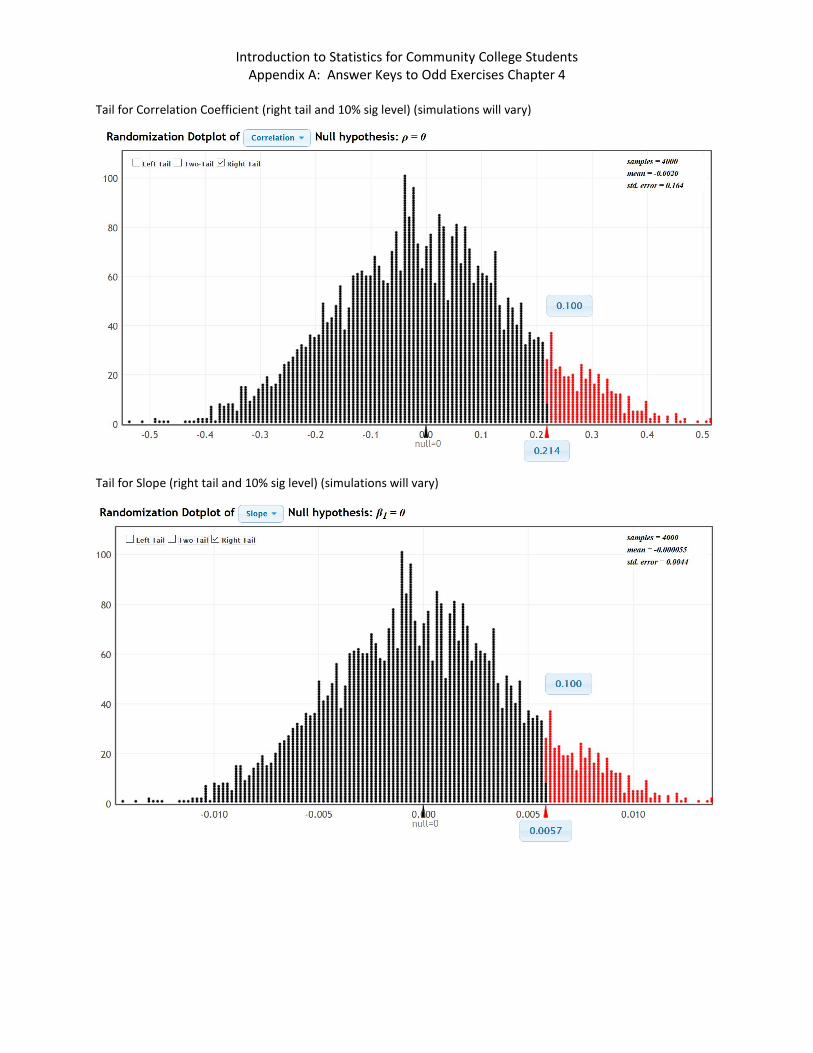
Introduction to Statistics for Community College Students Appendix A: Answer Keys to Odd Exercises Chapter 4
Tail for Correlation Coefficient (right tail and 10% sig level) (simulations will vary)
Tail for Slope (right tail and 10% sig level) (simulations will vary)

Introduction to Statistics for Community College Students Appendix A: Answer Keys to Odd Exercises Chapter 4
P-value calculation from slope simulation (answers will vary)
𝐻𝐻0: Population Slope (𝛽𝛽1) = 0 (No correlation)
𝐻𝐻𝐴𝐴: Population Slope (𝛽𝛽1) > 0 (Is positive correlation) CLAIM
The correlation coefficient (r) = 0.917
There is a strong positive correlation between the horsepower and weights of cars.
The correlation coefficient does fall in the tail determined by the correlation simulation and the 10% sig level.
The slope = 0.024
For every 1 horsepower increase in a car, the weights are increasing 0.024 tons on average.
The slope of 0.024 does fall in the tail determined by the slope simulation and the 10% sig level.
Sample data does significantly disagree with null hypothesis since the slope and correlation coefficient did fall in the tail determined by the simulations.
The slope of the regression line is significantly different (higher) than zero since the slope did fall in the tail determined by the simulation.
P-value (answer will vary) = 0 = 0%
P-value is lower than 10% significance level.
Unlikely to be sampling variability.
Reject the null hypothesis.

Introduction to Statistics for Community College Students Appendix A: Answer Keys to Odd Exercises Chapter 4
There is significant evidence to support the claim that there is a positive linear relationship (positive correlation) between the horsepower and weight of cars.
T-test statistic calculation (answers will vary) = (0.024 – 0) ÷ 0.0044 = 5.4545
The slope is 5.4545 standard errors above zero.
------------------------------------------------------------------------------------------------------------------------------------------
Chapter 4 Review Answers
1.
Correlation: Statistical analysis that determines if there is a relationship between two different quantitative variables.
Regression: Statistical analysis that involves finding the line or model that best fits a quantitative relationship, using the model to make predictions, and analyzing error in those predictions.
Explanatory Variable (𝑥𝑥): Another name for the x-variable or independent variable in a correlation study.
Response Variable (𝑦𝑦): Another name for the y-variable or dependent variable in a correlation study.
Correlation Coefficient (𝑟𝑟): A statistic between −1 and +1 that measures the strength and direction of linear relationships between two quantitative variables.
R-squared (𝑟𝑟2): Also called the coefficient of determination. This statistic measures the percent of variability in the y-variable that can be explained by the linear relationship with the x-variable.
Residual (𝑦𝑦 − 𝑦𝑦𝑦): The vertical distance between the regression line and a point in the scatterplot.
Standard Deviation of the Residual Errors (𝑠𝑠𝑏𝑏): A statistic that measures how far points in a scatterplot are from the regression line on average and measures the average amount of prediction error.
Slope (𝑏𝑏1): The amount of increase or decrease in the y-variable for every one-unit increase in the x-variable.
Y-Intercept (𝑏𝑏0): The predicted y-value when the x-value is zero.
Regression Line (𝑦𝑦� = 𝑏𝑏0 + 𝑏𝑏1𝑥𝑥): Also called the line of best fit or the line of least squares. This line minimizes the vertical distances between it and all the points in the scatterplot.
Scatterplot: A graph for visualizing the relationship between two quantitative ordered pair variables. The ordered pairs (𝑥𝑥,𝑦𝑦) are plotted on the rectangular coordinate system.
Residual Plot: A graph that pairs the residuals with the x values. This graph should be evenly spread out and not fan shaped.
Histogram of the Residuals: A graph showing the shape of the residuals. This graph should be nearly normal and centered close to zero.
Hypothesis Test: A procedure for testing a claim about a population.

Introduction to Statistics for Community College Students Appendix A: Answer Keys to Odd Exercises Chapter 4
Random Chance: Another word for sampling variability. The principle that random samples from the same population will usually be different and give very different statistics.
Critical Value: If the test statistic is higher than this number, then the sample data significantly disagrees with the null hypothesis. The z or t score critical values are also used to calculate margin of error in confidence intervals.
P-value: The probability of getting the sample data or more extreme by random chance if the null hypothesis is true. Significance Level (𝛼𝛼): Also called the Alpha Level. If the P-value is lower than this number, then the sample data significantly disagrees with the null hypothesis and is unlikely to have happened by random chance. This is also the probability of making a type 1 error. Randomized Simulation: A technique for visualizing sampling variability in a hypothesis test. The computer assumes the null hypothesis is true, and then generates random samples. If the sample data or test statistic falls in the tail, then the sample data significantly disagrees with the null hypothesis. This technique can also calculate the P-value without a formula.
Chi-square test statistic (χ²): The sum of the average of the squares of the differences between the observed sample counts and the expected counts from the null hypothesis.
F-test statistic: The ratio of the variance between the groups to the variance within the groups.
T-test statistic for correlation: The number of standard errors that the slope is above or below zero.
Z-test statistic for two-population proportion: The number of standard errors that the sample proportion from group 1 is above or below the sample proportion from group 2.
T-test statistic for two-population mean: The number of standard errors that the sample mean from group 1 is above or below the sample mean from group 2.
#2-4.
Two-population proportion test
𝐻𝐻0: 𝜋𝜋1 = 𝜋𝜋2
𝐻𝐻𝐴𝐴: 𝜋𝜋1 > 𝜋𝜋2
OR
𝐻𝐻0: 𝜋𝜋1 − 𝜋𝜋2 = 0
𝐻𝐻𝐴𝐴: 𝜋𝜋1 − 𝜋𝜋2 > 0
Z-test statistic
Assumptions: Random Samples, Individuals within and between the samples are independent, both samples have at least 10 success and at least 10 failures.
Goodness of Fit proportion test
𝐻𝐻0: 𝜋𝜋1 = 𝜋𝜋2 = 𝜋𝜋3 = 𝜋𝜋4
𝐻𝐻𝐴𝐴: at least one ≠

Introduction to Statistics for Community College Students Appendix A: Answer Keys to Odd Exercises Chapter 4
OR
𝐻𝐻0: 𝜋𝜋1 = 0.5, 𝜋𝜋2 = 0.25, 𝜋𝜋3 = 0.15, 𝜋𝜋4 = 0.1
𝐻𝐻𝐴𝐴: at least one ≠
Chi-square test statistic (χ²)
Assumptions: Random Samples, Individuals within and between the samples are independent, all expected counts are at least 5.
Categorical Association Test
𝐻𝐻0: Categorical variables are not related.
𝐻𝐻𝐴𝐴: Categorical variables are related.
Chi-square test statistic (χ²)
Assumptions: Random Sample or Random Samples, Individuals within (and between) the samples are independent, all expected counts are at least 5.
Two-population mean test
𝐻𝐻0: µ1 = µ2
𝐻𝐻𝐴𝐴: µ1 < µ2
OR
𝐻𝐻0: µ1 − µ2 = 0
𝐻𝐻𝐴𝐴: µ1 − µ2 < 0
OR
𝐻𝐻0: µ𝑑𝑑 = 0
𝐻𝐻𝐴𝐴: µ𝑑𝑑 < 0
T-test statistic for two-population mean.
Assumptions: Random Samples, Individuals within (and between) the samples are independent, both samples have a sample size of at least 30 or nearly normal.
ANOVA test
𝐻𝐻0: µ1 = µ2 = µ3 = µ4
𝐻𝐻𝐴𝐴: at least one ≠
F-test statistic
Assumptions: Random Samples, Individuals within (and between) the samples are independent, all samples have a sample size of at least 30 or nearly normal, sample standard deviations are close.
Correlation Test
𝐻𝐻0: Population Slope (𝛽𝛽1) = 0

Introduction to Statistics for Community College Students Appendix A: Answer Keys to Odd Exercises Chapter 4
𝐻𝐻𝐴𝐴: Population Slope (𝛽𝛽1) ≠ 0
OR
𝐻𝐻0: Population Correlation Coefficient (ρ) = 0
𝐻𝐻𝐴𝐴: Population Correlation Coefficient (ρ) ≠ 0
T-test statistic for correlation.
Assumptions: Quantitative ordered pair sample data collected randomly, Data values within the sample should be independent of each other, the sample size should be at least 30, the scatterplot and correlation coefficient (r) should show some linear pattern, there should be no influential outliers in the scatterplot, the histogram of the residuals should be nearly normal, the histogram of the residuals should be centered close to zero, the residual plot verses the x variables should be evenly spread out.
5.
Test Statistic Critical Value Does the sample data significantly disagree with 𝐻𝐻0? Explain why. F = 2.174 3.823 Not significantly disagree. Test stat not in tail.
T = −2.556 ± 1.96 Significantly disagree. Test stat in tail. 𝜒𝜒2 = 16.87 9.977 Significantly disagree. Test stat in tail. F = 5.339 2.742 Significantly disagree. Test stat in tail. T = 1.349 ± 2.576 Not significantly disagree. Test stat not in tail. 𝜒𝜒2 = 1.883 7.187 Not significantly disagree. Test stat not in tail.
6.
P-value P-value % Significance Level
Does the sample data significantly disagree with 𝐻𝐻0?
Could be random chance or Unlikely?
Reject 𝐻𝐻0 or fail to reject?
0.238 23.8% 5% Not Significantly disagree. Could be. Fail to reject 𝐻𝐻0
0.0003 0.03% 1% Significantly disagree. Unlikely Reject 𝐻𝐻0 5.7 x 10⁻⁶ 0.00057% 10% Significantly disagree. Unlikely Reject 𝐻𝐻0
0.441 44.1% 5% Not Significantly disagree. Could be. Fail to reject 𝐻𝐻0
0.138 13.8% 1% Not Significantly disagree. Could be. Fail to reject 𝐻𝐻0
0 0% 10% Significantly disagree. Unlikely Reject 𝐻𝐻0
7.
P-value Sig Level Claim Conclusion 0.238 5% 𝐻𝐻0 There is not significant evidence to reject the claim.
0.0003 1% 𝐻𝐻𝐴𝐴 There is significant evidence to support the claim. 5.7 x 10⁻⁶ 10% 𝐻𝐻0 There is significant evidence to reject the claim.
0.441 5% 𝐻𝐻𝐴𝐴 There is not significant evidence to support the claim. 0.138 1% 𝐻𝐻0 There is not significant evidence to reject the claim.
0 10% 𝐻𝐻𝐴𝐴 There is significant evidence to support the claim. 8.

Introduction to Statistics for Community College Students Appendix A: Answer Keys to Odd Exercises Chapter 4
Correlation Test
𝐻𝐻0: Population Slope (𝛽𝛽1) = 0
𝐻𝐻𝐴𝐴: Population Slope (𝛽𝛽1) ≠ 0
OR
𝐻𝐻0: Population Correlation Coefficient (ρ) = 0
𝐻𝐻𝐴𝐴: Population Correlation Coefficient (ρ) ≠ 0
T-test statistic for correlation.
Assumptions: Quantitative ordered pair sample data collected randomly, Data values within the sample should be independent of each other, the sample size should be at least 30, the scatterplot and correlation coefficient (r) should show some linear pattern, there should be no influential outliers in the scatterplot, the histogram of the residuals should be nearly normal, the histogram of the residuals should be centered close to zero, the residual plot verses the x variables should be evenly spread out.
9.
Categorical Association Test
𝐻𝐻0: Categorical variables are not related.
𝐻𝐻𝐴𝐴: Categorical variables are related.
Chi-square test statistic (χ²)
Assumptions: Random Sample or Random Samples, Individuals within (and between) the samples are independent, all expected counts are at least 5.
10.
ANOVA test
𝐻𝐻0: µ1 = µ2 = µ3 = µ4
𝐻𝐻𝐴𝐴: at least one ≠
F-test statistic
Assumptions: Random Samples, Individuals within (and between) the samples are independent, all samples have a sample size of at least 30 or nearly normal, sample standard deviations are close.
11.
Goodness of Fit proportion test
𝐻𝐻0: 𝜋𝜋1 = 𝜋𝜋2 = 𝜋𝜋3 = 𝜋𝜋4
𝐻𝐻𝐴𝐴: at least one ≠
OR
𝐻𝐻0: 𝜋𝜋1 = 0.5, 𝜋𝜋2 = 0.25, 𝜋𝜋3 = 0.15, 𝜋𝜋4 = 0.1
𝐻𝐻𝐴𝐴: at least one ≠

Introduction to Statistics for Community College Students Appendix A: Answer Keys to Odd Exercises Chapter 4
Chi-square test statistic (χ²)
Assumptions: Random Samples, Individuals within and between the samples are independent, all expected counts are at least 5.
12.
ANOVA since the amount of money is quantitative and the city is categorical.
13.
Goodness of Fit since we are checking a specific percentage in multiple groups.
14.
Correlation test since the amount of rainfall and number of fires are both quantitative variables.
15.
Categorical Association Test since the type of health insurance and the education level are both categorical variables with multiple responses.
16.
% of knee injuries from soccer = 31/100 = 31%
% of knee injuries from tennis = 5/100 = 5%
These percentages are significantly different indicating the sport may be related to having a knee injury.
Goodness of Fit test.
𝐻𝐻0: 𝜋𝜋1 = 𝜋𝜋2 = 𝜋𝜋3 = 𝜋𝜋4 = 𝜋𝜋5 = 𝜋𝜋6 (Claim)
𝐻𝐻𝐴𝐴: at least one ≠
Assumptions:
Random? Yes. Given
Individuals independent? Yes since it is a small random sample from a large population.
Expected counts at least 5? Yes. All expected counts are 16.7.
Chi-square test statistic = 28.16
Sample data significantly disagrees with null hypothesis since the test statistic falls in the tail determined by the critical value.
Observed sample counts significantly disagrees with expected counts in the null hypothesis since the test statistic falls in the tail determined by the critical value.
P-value = 0.0033869%
P-value is less than 1% significance level.
Unlikely to be sampling variability.
Reject the null hypothesis.

Introduction to Statistics for Community College Students Appendix A: Answer Keys to Odd Exercises Chapter 4
There is significant evidence to reject the claim that the percentage of knee injuries are the same in the various sports.
The data indicates that having a knee injury is related to the sport.
17.
% of raccoonss have rabies = 7/27 = 25.9%
% of squirrels have rabies = 17/38 = 44.7%
% of chipmunks have rabies = 8/30 = 26.7%
If these percentages are close, it would indicate that the type of animal is not related to having rabies.
If these percentages are significantly different, it would indicate that the type of animal is related to having rabies.
Categorical Association Test. (Since this data was collected from 1 random sample, it is sometimes referred to as “independence”.)
𝐻𝐻0: Rabies status is not related to the type of animal.
𝐻𝐻𝐴𝐴: Rabies status is related to the type of animal. (Claim)
Assumptions:
Random? Yes. Given
Individuals independent? It might not be independent if all the animals came from the same region.
Expected counts at least 5? Yes. The expected counts were 12.8, 10.11, 9.09, 25.2, 19.89, and 17.91.
Chi-square test statistic = 3.467
Sample data does NOT significantly disagrees with null hypothesis since the test statistic did NOT fall in the tail determined by the critical value.
Observed sample counts do NOT significantly disagree with expected counts in the null hypothesis since the test statistic did NOT fall in the tail determined by the critical value.
P-value = 17.67%
P-value is higher than 5% significance level.
Could be sampling variability.
Fail to reject the null hypothesis.
There is not significant evidence to support the claim that the type of animal is related to rabies status.
The data indicates that the type of animal may not be related to having rabies.

Introduction to Statistics for Community College Students Appendix A: Answer Keys to Odd Exercises Chapter 4
18.
Critical Value Calculations (Answers will vary.)

Introduction to Statistics for Community College Students Appendix A: Answer Keys to Odd Exercises Chapter 4
P-value Calculation (Answers will vary.)
% of males that believe in one true love = 372/1213 = 30.7%
% of females that believe in one true love = 363/1412 = 25.7%

Introduction to Statistics for Community College Students Appendix A: Answer Keys to Odd Exercises Chapter 4
If these percentages are close, it would indicate that gender is not related to believing in one true love.
If these percentages are significantly different, it would indicate that gender is related to believing in one true love.
Categorical Association Test.
𝐻𝐻0: Belief in one true love is not related to gender. (Claim)
𝐻𝐻𝐴𝐴: Belief in one true love is related to gender.
Assumptions:
Random? Unknown.
Individuals independent? If it is a random sample, then it probably is independent.
Expected counts at least 5? Yes. The expected counts were 339.6, 395.4, 837.3, 974.7, 36, and 42.
Chi-square test statistic = 7.989
Critical value (answer will vary) = 4.515
Sample data does significantly disagree with null hypothesis since the test statistic did fall in the tail determined by the critical value.
Observed sample counts do significantly disagree with expected counts in the null hypothesis since the test statistic did fall in the tail determined by the critical value.
P-value (answer will vary) = 0.015 = 1.5%
P-value is lower than 10% significance level.
Unlikely to be sampling variability.
Reject the null hypothesis.
There is significant evidence to reject the claim that gender is not related to believing in one true love.
The data indicates that gender is related to believing in one true love.
19.

Introduction to Statistics for Community College Students Appendix A: Answer Keys to Odd Exercises Chapter 4

Introduction to Statistics for Community College Students Appendix A: Answer Keys to Odd Exercises Chapter 4
𝐻𝐻0: µ1 = µ2 = µ3 = µ4 = µ5 (not related) CLAIM
𝐻𝐻𝐴𝐴: at least one ≠ (related)
Assumptions:
Random Samples? No. This data was a census. It may be representative though.
Individuals within (and between) the samples are independent? No. These students came from the same math 140 classes.
All samples have a sample size of at least 30 or nearly normal? Maybe. Shapes are unkown. All the sample sizes are above 30 except for twitter which was 29.
Sample standard deviations are close? No. One of the standard deviations (8) was more than twice as large as another (3.9).
F-test statistic = 0.437
Critical Value (answer will vary) = 2.368
Sample data does NOT significantly disagree with null hypothesis since the test statistic did NOT fall in the tail determined by the critical value.
The variance between the groups is NOT significantly higher than the variance within since the test statistic did NOT fall in the tail determined by the critical value.
P-value (answer will vary) = 0.780 = 78.0%
P-value is higher than 5% significance level.

Introduction to Statistics for Community College Students Appendix A: Answer Keys to Odd Exercises Chapter 4
Could be sampling variability.
Fail to reject the null hypothesis.
There is not significant evidence to reject the claim that the a persons favorite social media is not related to the money spent on meals.
The data indicates that social media might be NOT related to the money spent on meals. We do not have evidence and the data did not pass the assumptions.
20.
r = 0.7997
There is a strong positive correlation between the weights and BMI for the men in the sample.
𝑟𝑟2 = 0.6395 = 63.95%
63.95% of the variability in body mass index can be explained by the relationship with weight.
Slope = 0.1042
For every 1 pound increase in weight, the men’s BMI is increasing 0.1042 kg/𝑚𝑚2.
Y-intercept = 8.0169 (Does not make sense since it is impossible for a mans weight to be zero.)
If a man’s weight is zero pounds, the predicted BMI would be 8.0169 kg/𝑚𝑚2.
Standard Deviation of Residual Errors = 2.0869 kg/𝑚𝑚2.
The average prediction error is 2.0869 kg/𝑚𝑚2.
The average vertical distance from the regression line is 2.0869 kg/𝑚𝑚2.
Prediction for man weighing 185 pounds.
ŷ = 8.0169 + 0.1042X
ŷ = 8.0169 + 0.1042(185)
ŷ = 8.0169 + 19.277
ŷ = 27.2939 kg/𝑚𝑚2
(This prediction could have an average error of 2.0869 kg/𝑚𝑚2.)
Correlation Test
𝐻𝐻0: Population Slope (𝛽𝛽1) = 0 (No correlation)
𝐻𝐻𝐴𝐴: Population Slope (𝛽𝛽1) ≠ 0 (Is correlation) CLAIM
OR
𝐻𝐻0: Population Correlation Coefficient (ρ) = 0 (No correlation)
𝐻𝐻𝐴𝐴: Population Correlation Coefficient (ρ) ≠ 0 (Is correlation) CLAIM

Introduction to Statistics for Community College Students Appendix A: Answer Keys to Odd Exercises Chapter 4
Assumptions:
Quantitative ordered pair sample data collected randomly? Yes. Given
Data values within the sample should be independent of each other? Yes since it is a small random sample from a large population of all men.
The sample size should be at least 30? Yes. There are 40 men in the data.
The scatterplot and correlation coefficient (r) should show some linear pattern? Yes. The correlation coefficient and the scatterplot indicate a linear pattern. The correlation coefficient is not close to zero.
There should be no influential outliers in the scatterplot? Yes. The strong correlation coefficient and the scatterplot indicate no influential outliers.
The histogram of the residuals should be nearly normal? Yes. The histogram looks slightly skewed right, but can probably be thought of as nearly normal.
The histogram of the residuals should be centered close to zero? Yes. The highest bar in the histogram is touching the zero line.
The residual plot verses the x variables should be evenly spread out? Yes. There does not appear to be a drastic fan shape or sidewise V pattern. It is not perfectly even, but is close.
T-test statistic for correlation = 8.2095
Sample data does significantly disagree with null hypothesis since the test statistic did fall in the tail determined by the critical values.
The slope of the regression line is significantly different (higher) than zero since the test statistic did fall in the tail determined by the critical values.
P-value (answer will vary) = 0.00000000060619 = 0.000000060619%
P-value is lower than 1% significance level.
Unlikely to be sampling variability.
Reject the null hypothesis.
There is significant evidence to support the claim that there is a linear relationship (correlation) between the weight and BMI for men.
--------------------------------------------------------------------------------------------------------------------------------------------------------