Introduction to SystemC AMS

Martin Barnasconi, AMSWG chair

Outline

Introduction to SystemC AMS extensions

SystemC AMS 1.0 standard – language features

SystemC AMS 2.0 standard – language extensions

Summary and outlook

2

3

Introduction to SystemC AMS extensions

Introduction SystemC AMS extensions

Objectives of having a SystemC AMS language standard

- Unified and standardized modeling language to design and verify embedded

AMS systems

- Abstract AMS model descriptions supporting a design refinement

methodology, from functional specification to implementation

- AMS language constructs and semantics defined as C++ class library built on

top of IEEE Std 1666-2011 (SystemC LRM)

- Providing a modeling framework for development and exchange of AMS

intellectual property

- Foundation for development of AMS system level design tools

SystemC AMS extensions scope

- System-level language for analog and digital signal processing

- Integration of abstract AMS/RF subsystems in mixed-signal virtual prototypes

4

5

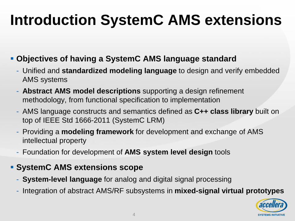
SystemC and AMS extensions

Specification

SystemC

SoC

Interface AMS D RF

missing

abstraction

SystemVerilog,

VHDL, Verilog

VHDL-AMS,

Verilog-AMS

Functional

Architecture

Implementation

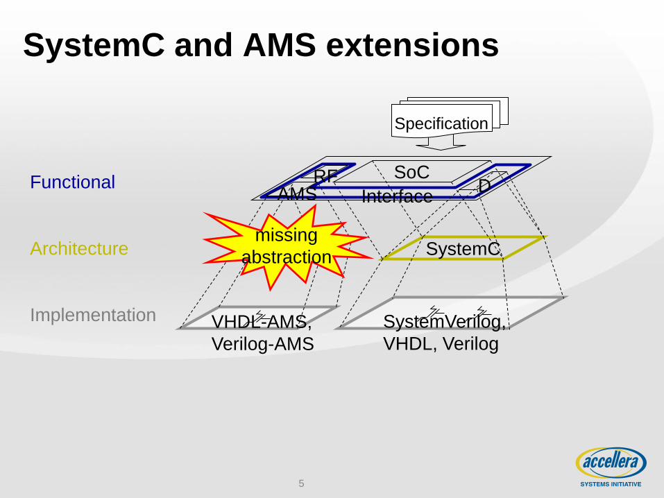
SystemC and AMS extensions

6

Specification

SystemC

SoC

Interface AMS D RF

SystemVerilog,

VHDL, Verilog

VHDL-AMS,

Verilog-AMS

SystemC

AMS extensions

Functional

Architecture

Implementation

2.0 2.3

7

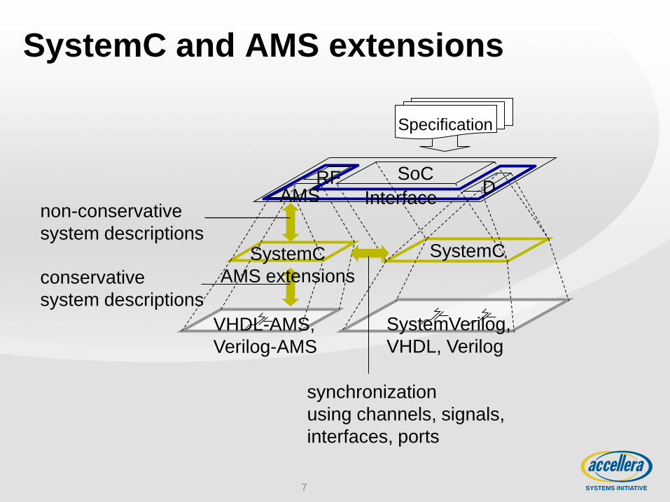
SystemC and AMS extensions

Specification

SystemC

SoC

Interface AMS D RF

VHDL-AMS,

Verilog-AMS

non-conservative

system descriptions

conservative

system descriptions

synchronization

using channels, signals,

interfaces, ports

SystemC

AMS extensions

SystemVerilog,

VHDL, Verilog

8

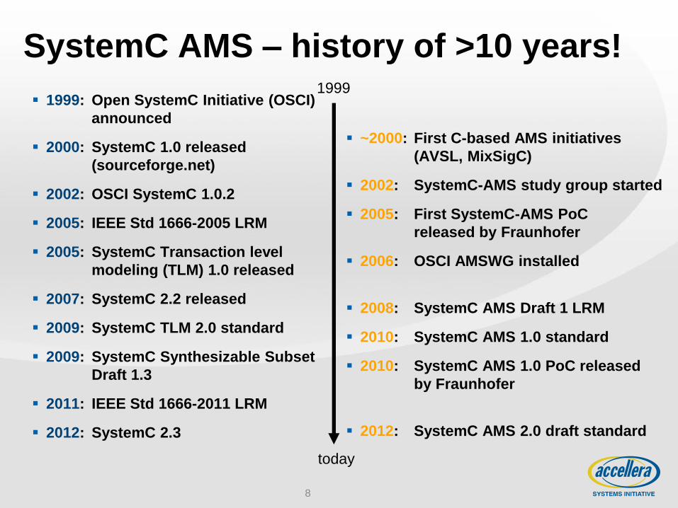
SystemC AMS – history of >10 years!

~2000: First C-based AMS initiatives

(AVSL, MixSigC)

2002: SystemC-AMS study group started

2005: First SystemC-AMS PoC

released by Fraunhofer

2006: OSCI AMSWG installed

2008: SystemC AMS Draft 1 LRM

2010: SystemC AMS 1.0 standard

2010: SystemC AMS 1.0 PoC released

by Fraunhofer

2012: SystemC AMS 2.0 draft standard

1999: Open SystemC Initiative (OSCI)

announced

2000: SystemC 1.0 released

(sourceforge.net)

2002: OSCI SystemC 1.0.2

2005: IEEE Std 1666-2005 LRM

2005: SystemC Transaction level

modeling (TLM) 1.0 released

2007: SystemC 2.2 released

2009: SystemC TLM 2.0 standard

2009: SystemC Synthesizable Subset

Draft 1.3

2011: IEEE Std 1666-2011 LRM

2012: SystemC 2.3

1999

today

SystemC AMS application focus

9

Image courtesy of STMicroelectronics

Automotive systems

Communication systems Imaging systems

10

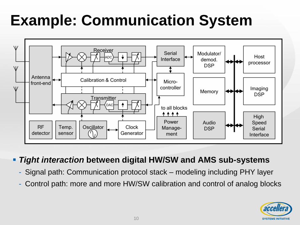
Example: Communication System

Tight interaction between digital HW/SW and AMS sub-systems

- Signal path: Communication protocol stack – modeling including PHY layer

- Control path: more and more HW/SW calibration and control of analog blocks

Receiver

Antenna

front-end

Serial

Interface Modulator/

demod.

DSP

Oscillator

Clock

Generator

Micro-

controller

Host

processor

Memory

Power

Manage-

ment

to all blocks

Audio

DSP

Imaging

DSP

ADC

Transmitter

DAC

RF

detector

Temp.

sensor

High

Speed

Serial

Interface

Calibration & Control

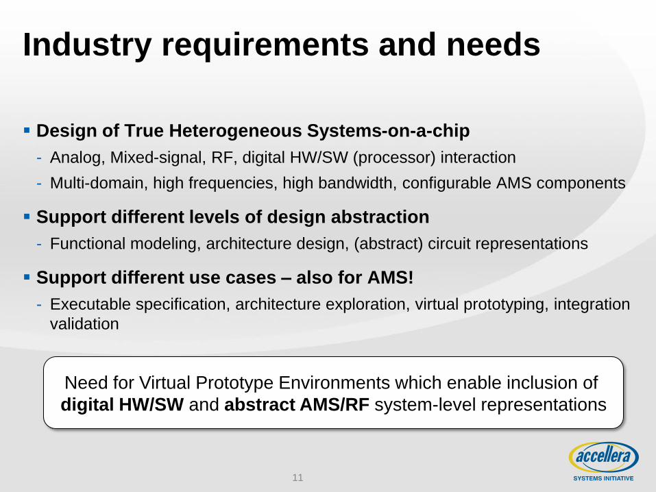
Industry requirements and needs

Design of True Heterogeneous Systems-on-a-chip

- Analog, Mixed-signal, RF, digital HW/SW (processor) interaction

- Multi-domain, high frequencies, high bandwidth, configurable AMS components

Support different levels of design abstraction

- Functional modeling, architecture design, (abstract) circuit representations

Support different use cases – also for AMS!

- Executable specification, architecture exploration, virtual prototyping, integration

validation

11

Need for Virtual Prototype Environments which enable inclusion of

digital HW/SW and abstract AMS/RF system-level representations

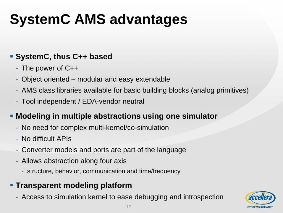
SystemC AMS advantages

SystemC, thus C++ based

- The power of C++

- Object oriented – modular and easy extendable

- AMS class libraries available for basic building blocks (analog primitives)

- Tool independent / EDA-vendor neutral

Modeling in multiple abstractions using one simulator

- No need for complex multi-kernel/co-simulation

- No difficult APIs

- Converter models and ports are part of the language

- Allows abstraction along four axis

- structure, behavior, communication and time/frequency

Transparent modeling platform

- Access to simulation kernel to ease debugging and introspection

12

13

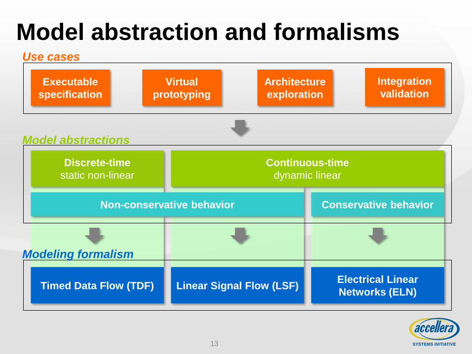
Model abstraction and formalisms

Timed Data Flow (TDF)

Modeling formalism

Use cases

Executable

specification

Architecture

exploration

Integration

validation Virtual

prototyping

Discrete-time

static non-linear

Non-conservative behavior

Model abstractions

Continuous-time

dynamic linear

Linear Signal Flow (LSF) Electrical Linear

Networks (ELN)

Conservative behavior

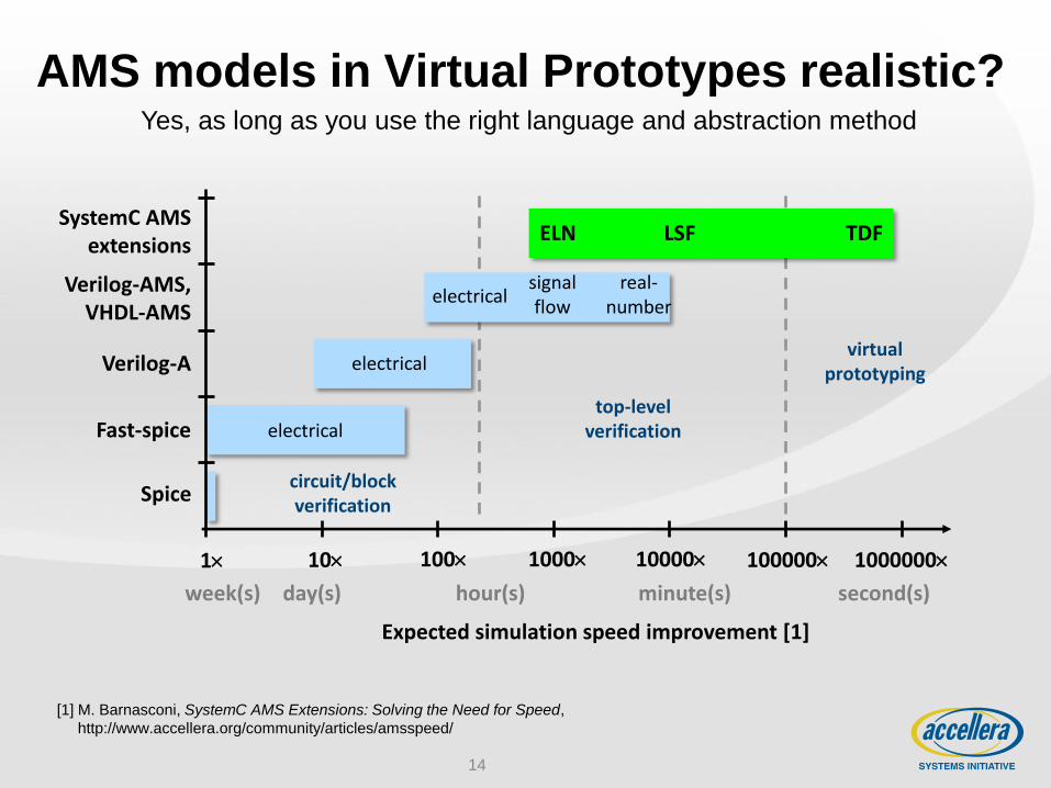
AMS models in Virtual Prototypes realistic?

14

1 10 100 1000 10000 100000

electrical

SystemC AMS extensions

Verilog-AMS, VHDL-AMS

Verilog-A

Fast-spice

Spice

real- number

electrical

electrical signal flow

ELN LSF TDF

Expected simulation speed improvement [1]

day(s) hour(s) minute(s) second(s) week(s)

1000000

circuit/block verification

virtual prototyping

top-level verification

Yes, as long as you use the right language and abstraction method

[1] M. Barnasconi, SystemC AMS Extensions: Solving the Need for Speed,

http://www.accellera.org/community/articles/amsspeed/

15

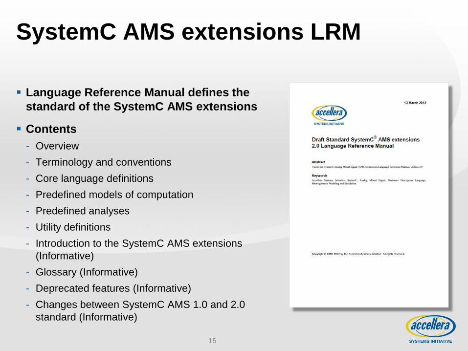
SystemC AMS extensions LRM

Language Reference Manual defines the

standard of the SystemC AMS extensions

Contents

- Overview

- Terminology and conventions

- Core language definitions

- Predefined models of computation

- Predefined analyses

- Utility definitions

- Introduction to the SystemC AMS extensions

(Informative)

- Glossary (Informative)

- Deprecated features (Informative)

- Changes between SystemC AMS 1.0 and 2.0

standard (Informative)

SystemC AMS User’s Guide

Comprehensive guide explaining the

basics of the AMS extensions

- TDF, LSF and ELN modeling

- Small-signal frequency-domain modeling

- Simulation and tracing

- Modeling strategy and refinement methodology

Many code examples

Application examples

- Binary Amplitude Shift Keying (BASK)

- Plain-Old-Telephone-System (POTS)

- Analog filters and networks

Has proven it’s value: reference guide for

many new users

16

SystemC AMS extensions User’s Guide

Abstract This is the SystemC Analog Mixed Signal (AMS) extensions User’s Guide.

Keywords Open SystemC Initiative, SystemC, Analog Mixed Signal, Heterogeneous Modeling and Simulation.

Copyright © 2009, 2010 by the Open SystemC Initiative (OSCI). All rights reserved.

March 8, 2010

17

SystemC AMS 1.0 standard

language features

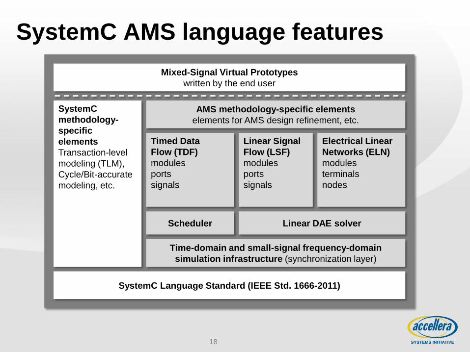
SystemC AMS language features

18

SystemC Language Standard (IEEE Std. 1666-2011)

Linear Signal

Flow (LSF)

modules

ports

signals

AMS methodology-specific elements

elements for AMS design refinement, etc.

Time-domain and small-signal frequency-domain

simulation infrastructure (synchronization layer)

Scheduler

Timed Data

Flow (TDF)

modules

ports

signals

Electrical Linear

Networks (ELN)

modules

terminals

nodes

Linear DAE solver

SystemC

methodology-

specific

elements

Transaction-level

modeling (TLM),

Cycle/Bit-accurate

modeling, etc.

Mixed-Signal Virtual Prototypes

written by the end user

19

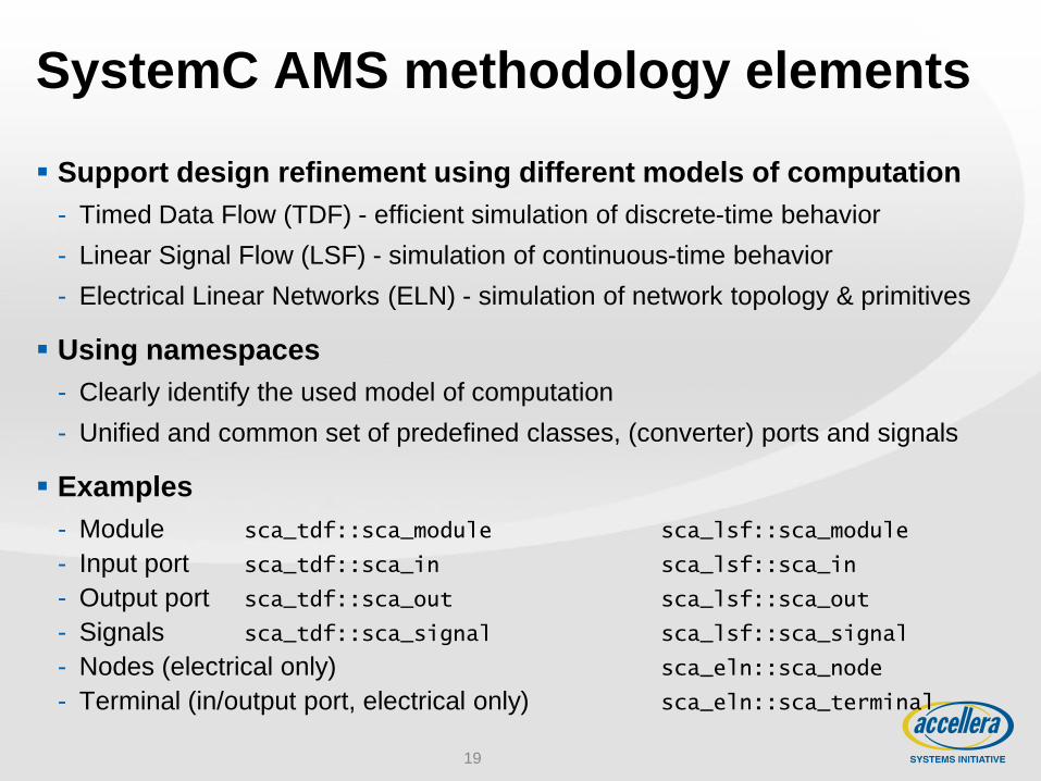
SystemC AMS methodology elements

Support design refinement using different models of computation

- Timed Data Flow (TDF) - efficient simulation of discrete-time behavior

- Linear Signal Flow (LSF) - simulation of continuous-time behavior

- Electrical Linear Networks (ELN) - simulation of network topology & primitives

Using namespaces

- Clearly identify the used model of computation

- Unified and common set of predefined classes, (converter) ports and signals

Examples

- Module sca_tdf::sca_module sca_lsf::sca_module

- Input port sca_tdf::sca_in sca_lsf::sca_in

- Output port sca_tdf::sca_out sca_lsf::sca_out

- Signals sca_tdf::sca_signal sca_lsf::sca_signal

- Nodes (electrical only) sca_eln::sca_node

- Terminal (in/output port, electrical only) sca_eln::sca_terminal

20

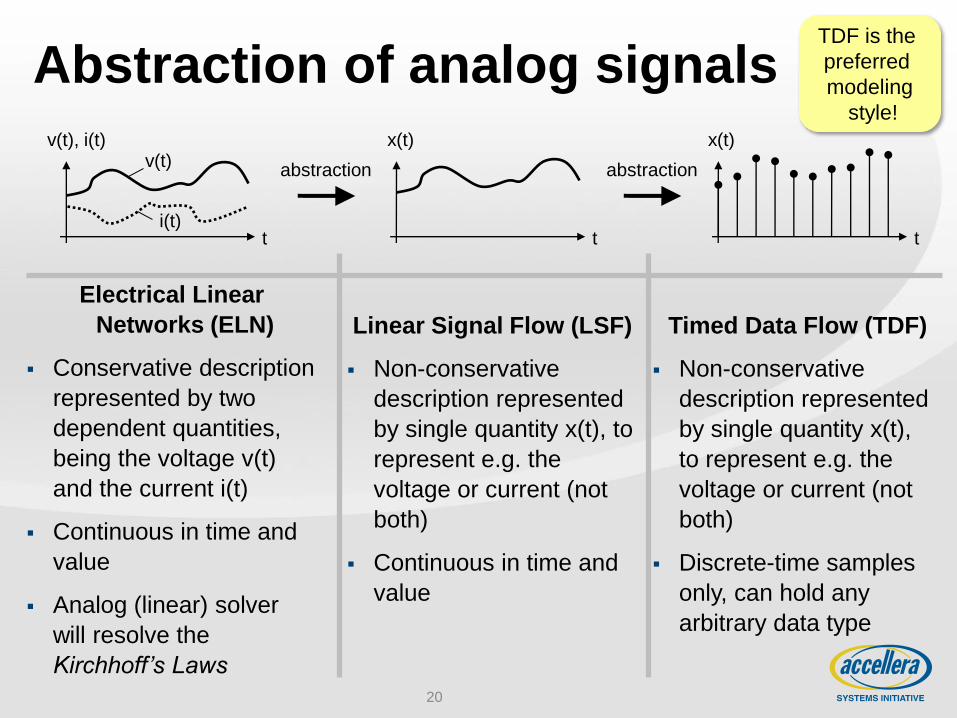
Abstraction of analog signals

t

v(t), i(t)

t

x(t)

t

x(t)

abstraction abstraction v(t)

i(t)

Linear Signal Flow (LSF)

Non-conservative

description represented

by single quantity x(t), to

represent e.g. the

voltage or current (not

both)

Continuous in time and

value

Timed Data Flow (TDF)

Non-conservative

description represented

by single quantity x(t),

to represent e.g. the

voltage or current (not

both)

Discrete-time samples

only, can hold any

arbitrary data type

Electrical Linear

Networks (ELN)

Conservative description

represented by two

dependent quantities,

being the voltage v(t)

and the current i(t)

Continuous in time and

value

Analog (linear) solver

will resolve the

Kirchhoff’s Laws

TDF is the

preferred

modeling

style!

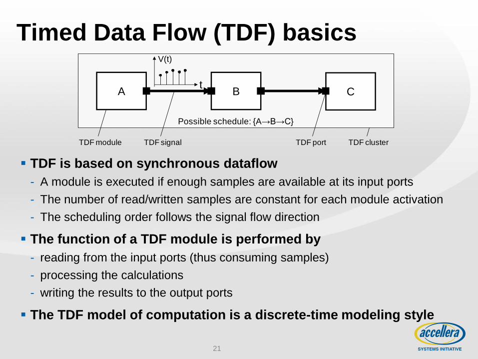
Timed Data Flow (TDF) basics

TDF is based on synchronous dataflow

- A module is executed if enough samples are available at its input ports

- The number of read/written samples are constant for each module activation

- The scheduling order follows the signal flow direction

The function of a TDF module is performed by

- reading from the input ports (thus consuming samples)

- processing the calculations

- writing the results to the output ports

The TDF model of computation is a discrete-time modeling style

21

Possible schedule: {A→B→C}

t

V(t)

outCA B

TDF module TDF portTDF signal TDF cluster

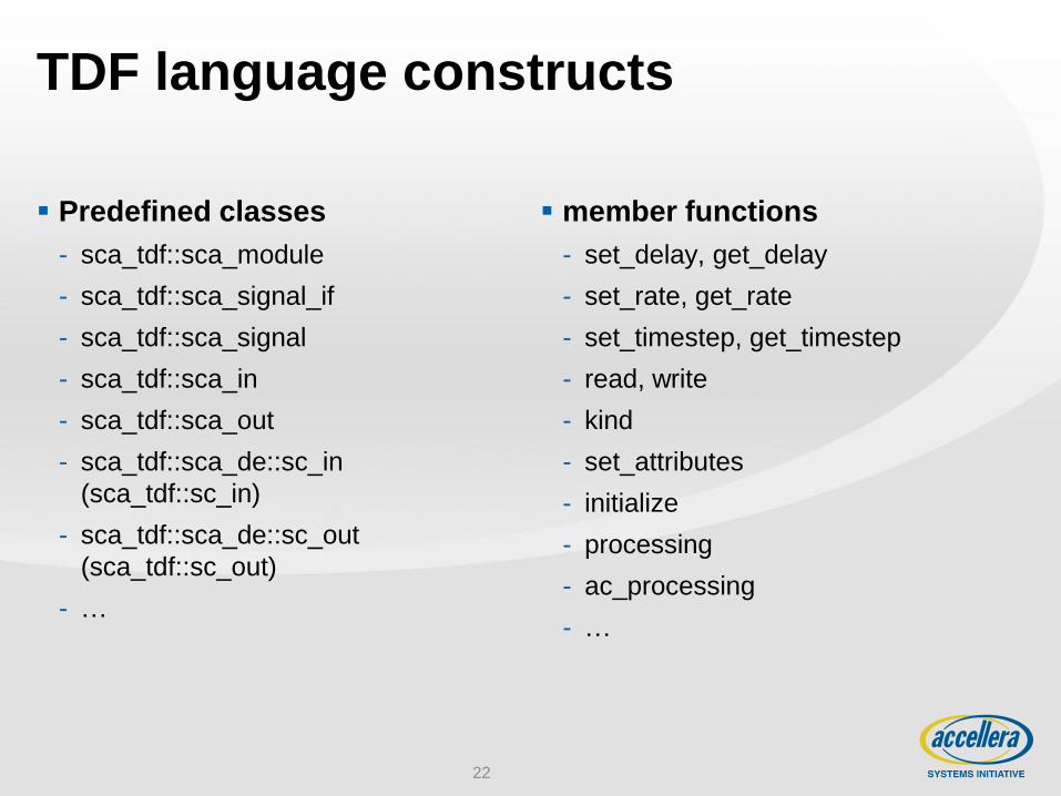
TDF language constructs

Predefined classes

- sca_tdf::sca_module

- sca_tdf::sca_signal_if

- sca_tdf::sca_signal

- sca_tdf::sca_in

- sca_tdf::sca_out

- sca_tdf::sca_de::sc_in

(sca_tdf::sc_in)

- sca_tdf::sca_de::sc_out

(sca_tdf::sc_out)

- …

member functions

- set_delay, get_delay

- set_rate, get_rate

- set_timestep, get_timestep

- read, write

- kind

- set_attributes

- initialize

- processing

- ac_processing

- …

22

23

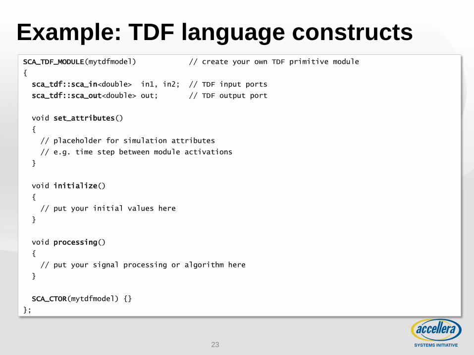
Example: TDF language constructs SCA_TDF_MODULE(mytdfmodel) // create your own TDF primitive module

{

sca_tdf::sca_in<double> in1, in2; // TDF input ports

sca_tdf::sca_out<double> out; // TDF output port

void set_attributes()

{

// placeholder for simulation attributes

// e.g. time step between module activations

}

void initialize()

{

// put your initial values here

}

void processing()

{

// put your signal processing or algorithm here

}

SCA_CTOR(mytdfmodel) {}

};

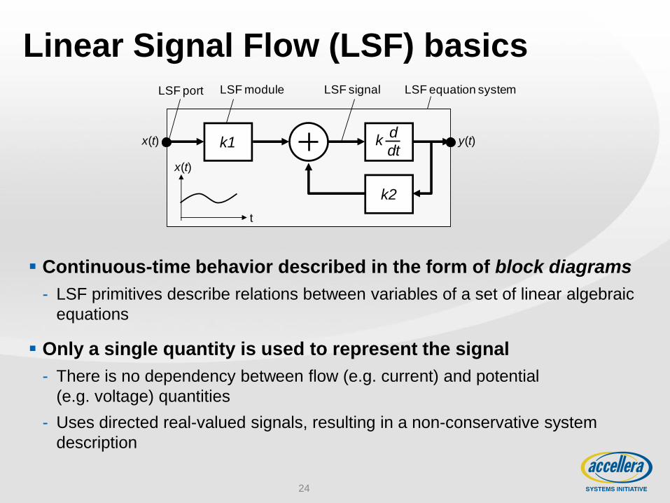
Linear Signal Flow (LSF) basics

Continuous-time behavior described in the form of block diagrams

- LSF primitives describe relations between variables of a set of linear algebraic

equations

Only a single quantity is used to represent the signal

- There is no dependency between flow (e.g. current) and potential

(e.g. voltage) quantities

- Uses directed real-valued signals, resulting in a non-conservative system

description

24

t

k1

LSF module LSF signalLSF port LSF equation system

k2

x(t) y(t)kd

dtx(t)

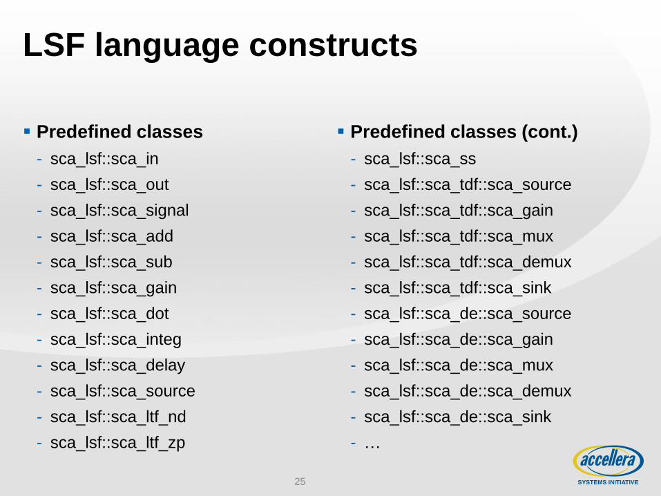
LSF language constructs

Predefined classes

- sca_lsf::sca_in

- sca_lsf::sca_out

- sca_lsf::sca_signal

- sca_lsf::sca_add

- sca_lsf::sca_sub

- sca_lsf::sca_gain

- sca_lsf::sca_dot

- sca_lsf::sca_integ

- sca_lsf::sca_delay

- sca_lsf::sca_source

- sca_lsf::sca_ltf_nd

- sca_lsf::sca_ltf_zp

Predefined classes (cont.)

- sca_lsf::sca_ss

- sca_lsf::sca_tdf::sca_source

- sca_lsf::sca_tdf::sca_gain

- sca_lsf::sca_tdf::sca_mux

- sca_lsf::sca_tdf::sca_demux

- sca_lsf::sca_tdf::sca_sink

- sca_lsf::sca_de::sca_source

- sca_lsf::sca_de::sca_gain

- sca_lsf::sca_de::sca_mux

- sca_lsf::sca_de::sca_demux

- sca_lsf::sca_de::sca_sink

- …

25

26

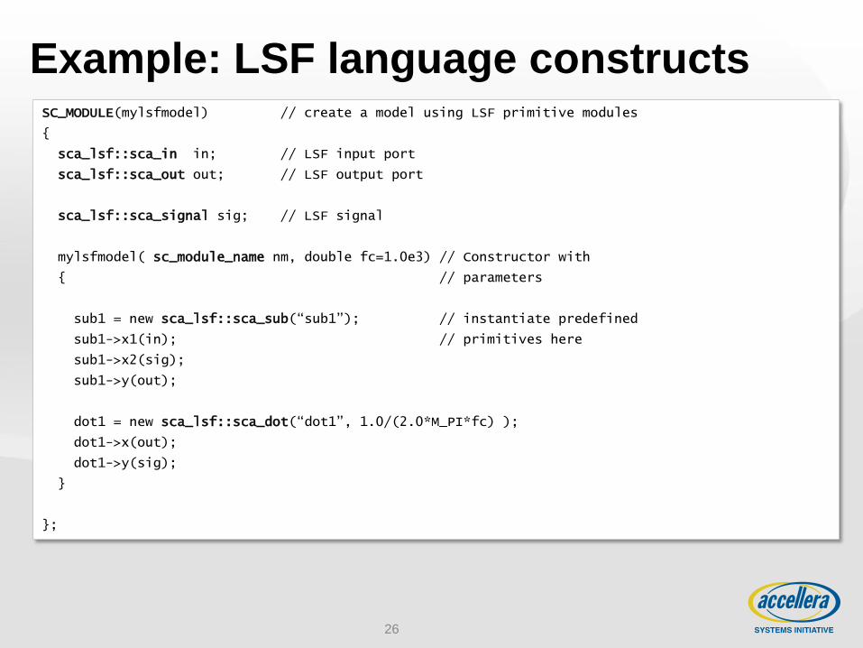
Example: LSF language constructs SC_MODULE(mylsfmodel) // create a model using LSF primitive modules

{

sca_lsf::sca_in in; // LSF input port

sca_lsf::sca_out out; // LSF output port

sca_lsf::sca_signal sig; // LSF signal

mylsfmodel( sc_module_name nm, double fc=1.0e3) // Constructor with

{ // parameters

sub1 = new sca_lsf::sca_sub(“sub1”); // instantiate predefined

sub1->x1(in); // primitives here

sub1->x2(sig);

sub1->y(out);

dot1 = new sca_lsf::sca_dot(“dot1”, 1.0/(2.0*M_PI*fc) );

dot1->x(out);

dot1->y(sig);

}

};

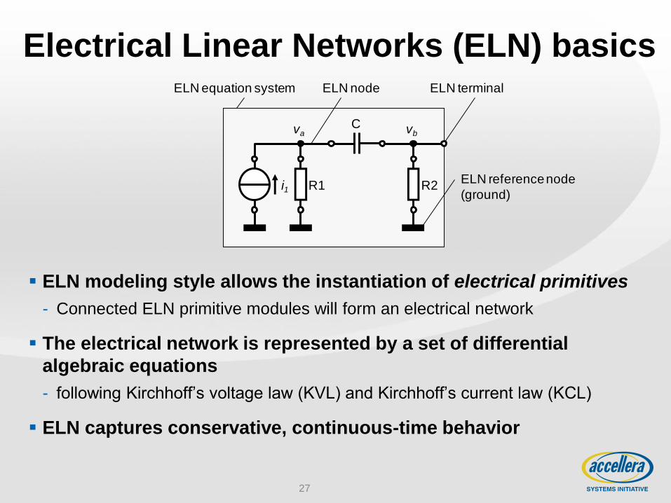
Electrical Linear Networks (ELN) basics

ELN modeling style allows the instantiation of electrical primitives

- Connected ELN primitive modules will form an electrical network

The electrical network is represented by a set of differential

algebraic equations

- following Kirchhoff’s voltage law (KVL) and Kirchhoff’s current law (KCL)

ELN captures conservative, continuous-time behavior

27

ELN node ELN terminalELN equation system

va

R1i1

C

R2

vb

ELN reference node

(ground)

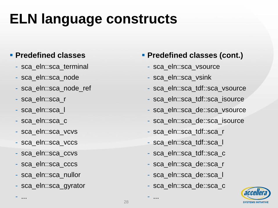
ELN language constructs

Predefined classes

- sca_eln::sca_terminal

- sca_eln::sca_node

- sca_eln::sca_node_ref

- sca_eln::sca_r

- sca_eln::sca_l

- sca_eln::sca_c

- sca_eln::sca_vcvs

- sca_eln::sca_vccs

- sca_eln::sca_ccvs

- sca_eln::sca_cccs

- sca_eln::sca_nullor

- sca_eln::sca_gyrator

- ...

Predefined classes (cont.)

- sca_eln::sca_vsource

- sca_eln::sca_vsink

- sca_eln::sca_tdf::sca_vsource

- sca_eln::sca_tdf::sca_isource

- sca_eln::sca_de::sca_vsource

- sca_eln::sca_de::sca_isource

- sca_eln::sca_tdf::sca_r

- sca_eln::sca_tdf::sca_l

- sca_eln::sca_tdf::sca_c

- sca_eln::sca_de::sca_r

- sca_eln::sca_de::sca_l

- sca_eln::sca_de::sca_c

- ... 28

29

Example: ELN language constructs SC_MODULE(myelnmodel) // model using ELN primitive modules

{

sca_eln::sca_terminal in, out; // ELN terminal (input and output)

sca_eln::sca_node_ref gnd; // ELN reference node

SC_CTOR(myelnmodel) // standard constructor

{

r1 = new sca_eln::sca_r(“r1”, 10e3); // instantiate predefined

r1->p(in); // primitive here (resistor)

r1->n(out);

c1 = new sca_eln::sca_c(“c1”, 100e-6);

c1->p(out);

c1->n(gnd);

}

};

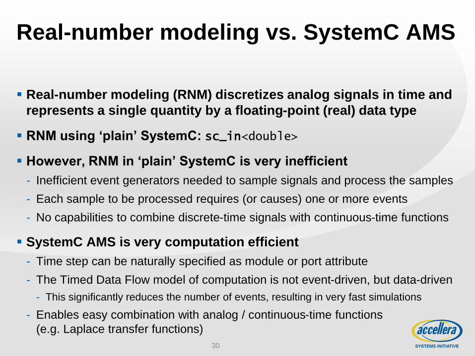
Real-number modeling vs. SystemC AMS

Real-number modeling (RNM) discretizes analog signals in time and

represents a single quantity by a floating-point (real) data type

RNM using ‘plain’ SystemC: sc_in<double>

However, RNM in ‘plain’ SystemC is very inefficient

- Inefficient event generators needed to sample signals and process the samples

- Each sample to be processed requires (or causes) one or more events

- No capabilities to combine discrete-time signals with continuous-time functions

SystemC AMS is very computation efficient

- Time step can be naturally specified as module or port attribute

- The Timed Data Flow model of computation is not event-driven, but data-driven

- This significantly reduces the number of events, resulting in very fast simulations

- Enables easy combination with analog / continuous-time functions

(e.g. Laplace transfer functions)

30

31

SystemC AMS 2.0 standard

language extensions

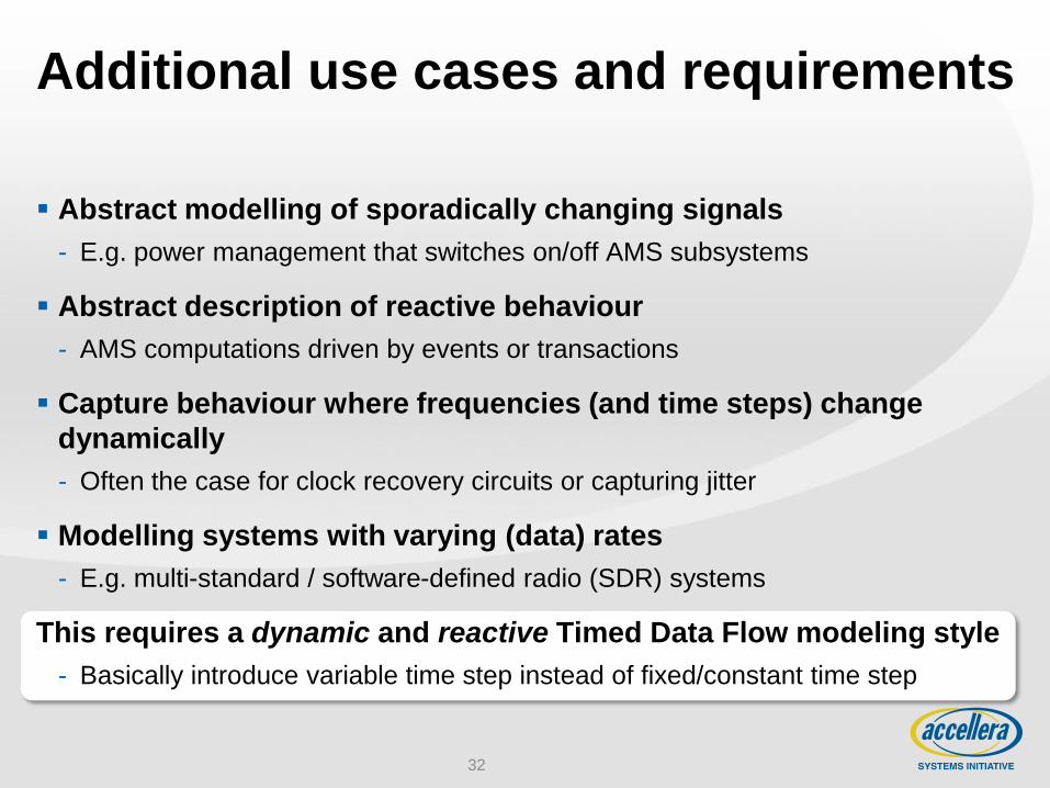
Additional use cases and requirements

Abstract modelling of sporadically changing signals

- E.g. power management that switches on/off AMS subsystems

Abstract description of reactive behaviour

- AMS computations driven by events or transactions

Capture behaviour where frequencies (and time steps) change

dynamically

- Often the case for clock recovery circuits or capturing jitter

Modelling systems with varying (data) rates

- E.g. multi-standard / software-defined radio (SDR) systems

This requires a dynamic and reactive Timed Data Flow modeling style

- Basically introduce variable time step instead of fixed/constant time step

32

Use cases and requirements overview

33

Use cases Requirements Application examples

Abstraction of sporadically changing signals

Switch on/off AMS computations

Power management unit

Abstract description of reactive behavior

Detect analog zero- or threshold crossing

Sensor circuits; alarm mode of systems

Request and response caused by digital event or

transaction

AMS embedded in digital HW/SW virtual prototype

Capture behavior where frequencies (and

time steps) change dynamically

Changeable time step of AMS computations

VCO, PLL, PWM, Clock recovery circuits

Modeling systems with varying (data) rates

Changeable time step and/or data rate

Communication systems, multi-standard radio

interfaces (e.g. cognitive radios)

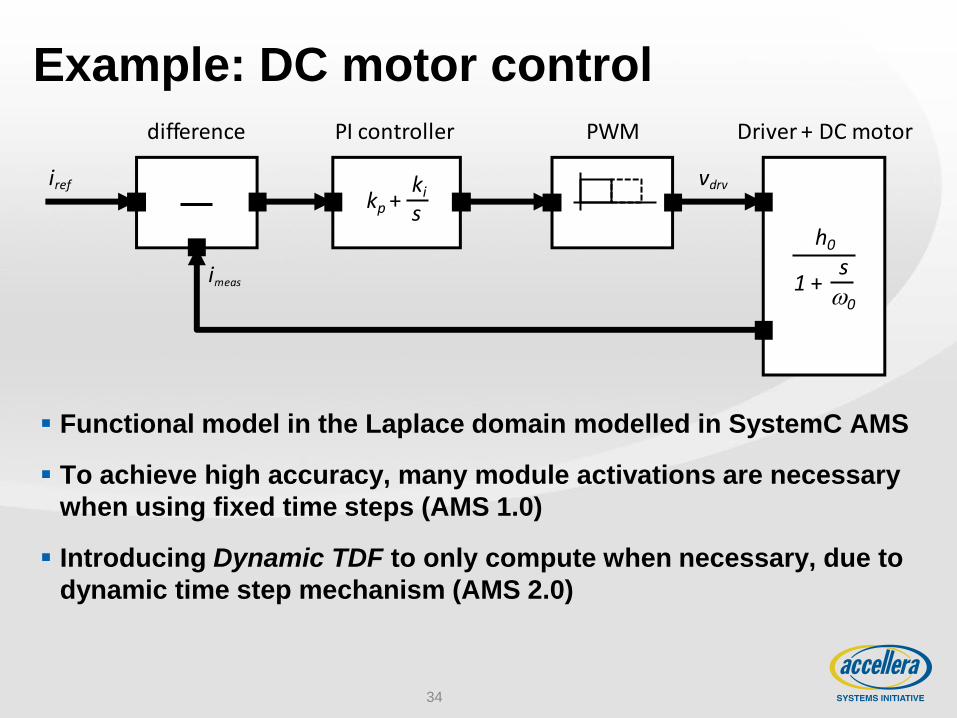
Example: DC motor control

Functional model in the Laplace domain modelled in SystemC AMS

To achieve high accuracy, many module activations are necessary

when using fixed time steps (AMS 1.0)

Introducing Dynamic TDF to only compute when necessary, due to

dynamic time step mechanism (AMS 2.0)

34

outiref

imeas

PI controllerdifference

kp +ki

s

PWM Driver + DC motor

1 +s0

h0

vdrv

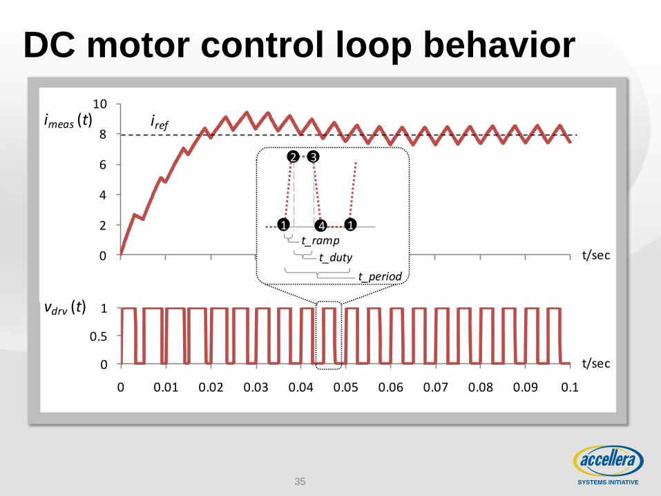
DC motor control loop behavior

35

0

2

4

6

8

10

0 0.01 0.02 0.03 0.04 0.05 0.06 0.07 0.08 0.09 0.1

0

0.5

1

0 0.01 0.02 0.03 0.04 0.05 0.06 0.07 0.08 0.09 0.1

t/sec

t/sec

imeas (t)

vdrv (t)

iref

t_ramp1

2 3

4 1

t_duty

t_period

Dynamic TDF features in AMS 2.0

New callback and member functions to support Dynamic TDF:

change_attributes()

- callback provides a context, in which the time step, rate, or delay attributes of a

TDF cluster may be changed

request_next_activation(…)

- member function to request a next cluster activation at a given time step, event,

or event-list

does_attribute_changes(), does_no_attribute_changes()

- member functions to mark a TDF module to allow or disallow making attribute

changes itself, respectively

accept_attribute_changes(), reject_attribute_changes()

- member functions to mark a TDF module to accept or reject attribute changes

caused by other TDF modules, respectively

36

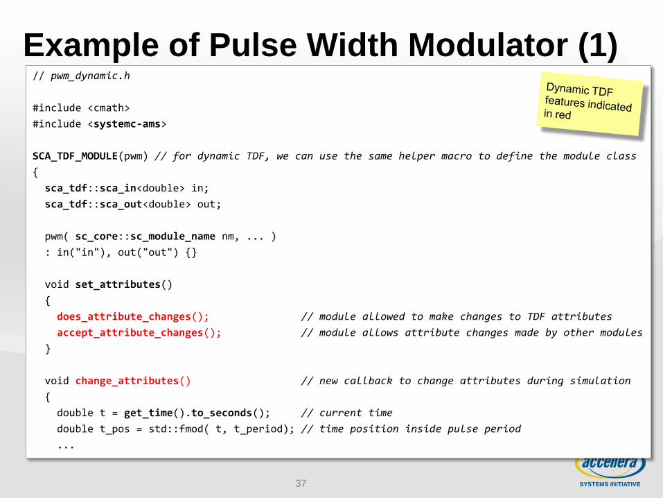
Example of Pulse Width Modulator (1)

37

// pwm_dynamic.h

#include <cmath>

#include <systemc-ams>

SCA_TDF_MODULE(pwm) // for dynamic TDF, we can use the same helper macro to define the module class

{

sca_tdf::sca_in<double> in;

sca_tdf::sca_out<double> out;

pwm( sc_core::sc_module_name nm, ... )

: in("in"), out("out") {}

void set_attributes()

{

does_attribute_changes(); // module allowed to make changes to TDF attributes

accept_attribute_changes(); // module allows attribute changes made by other modules

}

void change_attributes() // new callback to change attributes during simulation

{

double t = get_time().to_seconds(); // current time

double t_pos = std::fmod( t, t_period); // time position inside pulse period

...

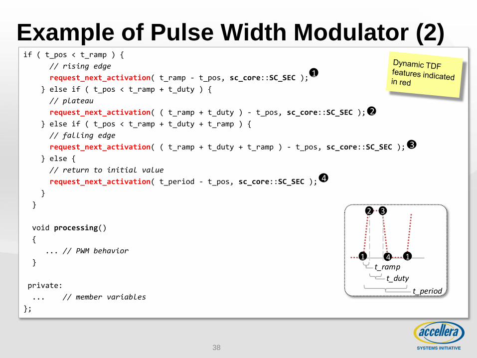
Example of Pulse Width Modulator (2)

38

if ( t_pos < t_ramp ) {

// rising edge

request_next_activation( t_ramp - t_pos, sc_core::SC_SEC );

} else if ( t_pos < t_ramp + t_duty ) {

// plateau

request_next_activation( ( t_ramp + t_duty ) - t_pos, sc_core::SC_SEC );

} else if ( t_pos < t_ramp + t_duty + t_ramp ) {

// falling edge

request_next_activation( ( t_ramp + t_duty + t_ramp ) - t_pos, sc_core::SC_SEC );

} else {

// return to initial value

request_next_activation( t_period - t_pos, sc_core::SC_SEC );

}

}

void processing()

{

... // PWM behavior

}

private:

... // member variables

};

t_ramp1

2 3

4 1

t_duty

t_period

1

2

3

4

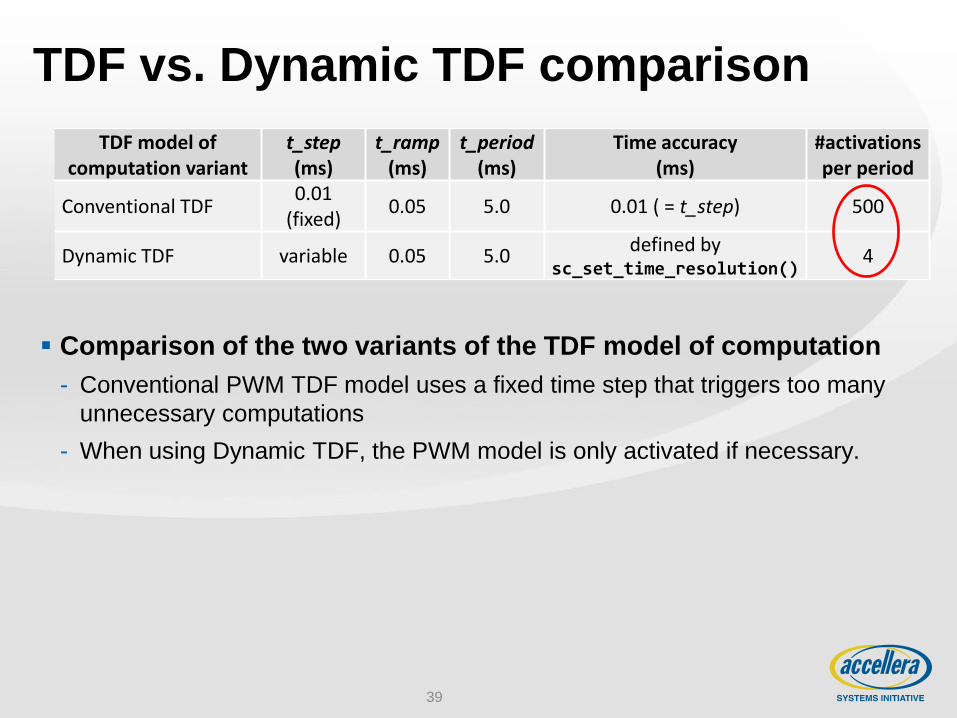
TDF vs. Dynamic TDF comparison

39

TDF model of computation variant

t_step (ms)

t_ramp (ms)

t_period (ms)

Time accuracy (ms)

#activations per period

Conventional TDF 0.01

(fixed) 0.05 5.0 0.01 ( = t_step) 500

Dynamic TDF variable 0.05 5.0 defined by

sc_set_time_resolution() 4

Comparison of the two variants of the TDF model of computation

- Conventional PWM TDF model uses a fixed time step that triggers too many

unnecessary computations

- When using Dynamic TDF, the PWM model is only activated if necessary.

Summary and outlook

SystemC AMS developments are fully driven and supported by

European industry: NXP, ST, Infineon, and Continental

SystemC AMS 1.0 standard was released in March 2010

SystemC AMS 2.0 standard released in March 2013

- Introducing Dynamic Timed Data Flow to facilitate a more reactive and dynamic

behavior for AMS computations

Third party Proof-of-Concept implementation for SystemC AMS 1.0

available under Apache 2.0 license

- Thanks to Fraunhofer IIS/EAS Dresden

Discussions ongoing with EDA vendors for commercial tool support

40

More information

www.accellera.org

www.accellera.org/downloads/standards/systemc/ams

www.accellera.org/community/articles/amsspeed

www.accellera.org/community/articles/amsdynamictdf

www.systemc-ams.org

41

Thank you

43

Back-up

Simple code example:

Top-level RF frontend module

44

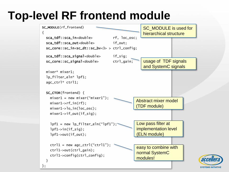
Top-level RF frontend module SC_MODULE(rf_frontend)

{

sca_tdf::sca_in<double> rf, loc_osc;

sca_tdf::sca_out<double> if_out;

sc_core::sc_in<sc_dt::sc_bv<3> > ctrl_config;

sca_tdf::sca_signal<double> if_sig;

sc_core::sc_signal<double> ctrl_gain;

mixer* mixer1;

lp_filter_eln* lpf1;

agc_ctrl* ctrl1;

SC_CTOR(frontend) {

mixer1 = new mixer(“mixer1”);

mixer1->rf_in(rf);

mixer1->lo_in(loc_osc);

mixer1->if_out(if_sig);

lpf1 = new lp_filter_eln(“lpf1”);

lpf1->in(if_sig);

lpf1->out(if_out);

ctrl1 = new agc_ctrl(“ctrl1”);

ctrl1->out(ctrl_gain);

ctrl1->config(ctrl_config);

}

};

SC_MODULE is used for

hierarchical structure

usage of TDF signals

and SystemC signals

Abstract mixer model

(TDF module)

Low pass filter at

implementation level

(ELN module)

easy to combine with

normal SystemC

modules!

45

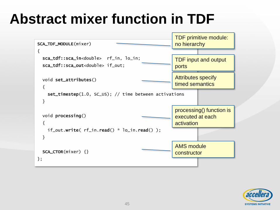
Abstract mixer function in TDF

SCA_TDF_MODULE(mixer)

{

sca_tdf::sca_in<double> rf_in, lo_in;

sca_tdf::sca_out<double> if_out;

void set_attributes()

{

set_timestep(1.0, SC_US); // time between activations

}

void processing()

{

if_out.write( rf_in.read() * lo_in.read() );

}

SCA_CTOR(mixer) {}

};

TDF primitive module:

no hierarchy

TDF input and output

ports

Attributes specify

timed semantics

processing() function is

executed at each

activation

AMS module

constructor

46

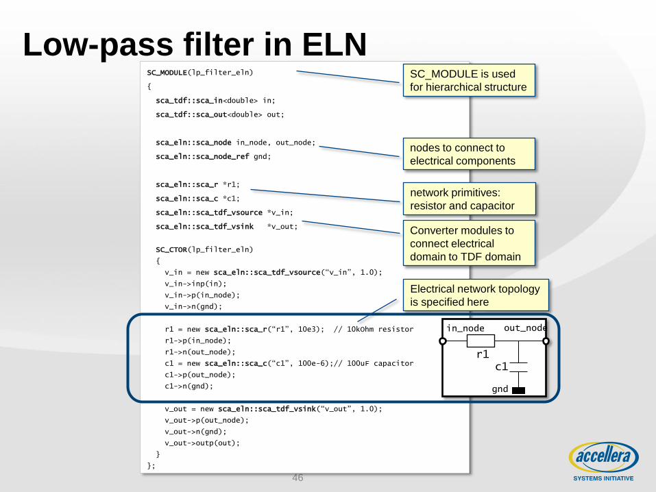
Low-pass filter in ELN SC_MODULE(lp_filter_eln)

{

sca_tdf::sca_in<double> in;

sca_tdf::sca_out<double> out;

sca_eln::sca_node in_node, out_node;

sca_eln::sca_node_ref gnd;

sca_eln::sca_r *r1;

sca_eln::sca_c *c1;

sca_eln::sca_tdf_vsource *v_in;

sca_eln::sca_tdf_vsink *v_out;

SC_CTOR(lp_filter_eln)

{

v_in = new sca_eln::sca_tdf_vsource(“v_in”, 1.0);

v_in->inp(in);

v_in->p(in_node);

v_in->n(gnd);

r1 = new sca_eln::sca_r(“r1”, 10e3); // 10kOhm resistor

r1->p(in_node);

r1->n(out_node);

c1 = new sca_eln::sca_c(“c1”, 100e-6);// 100uF capacitor

c1->p(out_node);

c1->n(gnd);

v_out = new sca_eln::sca_tdf_vsink(“v_out”, 1.0);

v_out->p(out_node);

v_out->n(gnd);

v_out->outp(out);

}

};

SC_MODULE is used

for hierarchical structure

nodes to connect to

electrical components

network primitives:

resistor and capacitor

Converter modules to

connect electrical

domain to TDF domain

actual

network

topology

r1 c1

gnd

out_node in_node

Electrical network topology

is specified here