introduction to tensor calculus - arxiv.org · introduction to tensor calculus taha sochi may 25,...
TRANSCRIPT

Introduction to Tensor Calculus
Taha Sochi∗
May 25, 2016
∗Department of Physics & Astronomy, University College London, Gower Street, London, WC1E 6BT.
Email: [email protected].
1
arX
iv:1
603.
0166
0v3
[m
ath.
HO
] 2
3 M
ay 2
016
2
Preface
These are general notes on tensor calculus originated from a collection of personal notes
which I prepared some time ago for my own use and reference when I was studying the
subject. I decided to put them in the public domain hoping they may be beneficial to some
students in their effort to learn this subject. Most of these notes were prepared in the
form of bullet points like tutorials and presentations and hence some of them may be more
concise than they should be. Moreover, some notes may not be sufficiently thorough or
general. However this should be understandable considering the level and original purpose
of these notes and the desire for conciseness. There may also be some minor repetition
in some places for the purpose of gathering similar items together, or emphasizing key
points, or having self-contained sections and units.
These notes, in my view, can be used as a short reference for an introductory course on
tensor algebra and calculus. I assume a basic knowledge of calculus and linear algebra
with some commonly used mathematical terminology. I tried to be as clear as possible and
to highlight the key issues of the subject at an introductory level in a concise form. I hope
I have achieved some success in reaching these objectives at least for some of my target
audience. The present text is supposed to be the first part of a series of documents about
tensor calculus for gradually increasing levels or tiers. I hope I will be able to finalize and
publicize the document for the next level in the near future.
CONTENTS 3
Contents
Preface 2
Contents 3
1 Notation, Nomenclature and Conventions 5
2 Preliminaries 10
2.1 Introduction . . . . . . . . . . . . . . . . . . . . . . . . . . . . . . . . . . . 10
2.2 General Rules . . . . . . . . . . . . . . . . . . . . . . . . . . . . . . . . . 12
2.3 Examples of Tensors of Different Ranks . . . . . . . . . . . . . . . . . . . . 15
2.4 Applications of Tensors . . . . . . . . . . . . . . . . . . . . . . . . . . . . . 16
2.5 Types of Tensors . . . . . . . . . . . . . . . . . . . . . . . . . . . . . . . . 17
2.5.1 Covariant and Contravariant Tensors . . . . . . . . . . . . . . . . . 17
2.5.2 True and Pseudo Tensors . . . . . . . . . . . . . . . . . . . . . . . . 22
2.5.3 Absolute and Relative Tensors . . . . . . . . . . . . . . . . . . . . . 24
2.5.4 Isotropic and Anisotropic Tensors . . . . . . . . . . . . . . . . . . . 25
2.5.5 Symmetric and Anti-symmetric Tensors . . . . . . . . . . . . . . . . 25
2.6 Tensor Operations . . . . . . . . . . . . . . . . . . . . . . . . . . . . . . . 28
2.6.1 Addition and Subtraction . . . . . . . . . . . . . . . . . . . . . . . 28
2.6.2 Multiplication by Scalar . . . . . . . . . . . . . . . . . . . . . . . . 29
2.6.3 Tensor Multiplication . . . . . . . . . . . . . . . . . . . . . . . . . 30
2.6.4 Contraction . . . . . . . . . . . . . . . . . . . . . . . . . . . . . . . 31
2.6.5 Inner Product . . . . . . . . . . . . . . . . . . . . . . . . . . . . . . 32
2.6.6 Permutation . . . . . . . . . . . . . . . . . . . . . . . . . . . . . . . 34
2.7 Tensor Test: Quotient Rule . . . . . . . . . . . . . . . . . . . . . . . . . . 34
CONTENTS 4
3 δ and ε Tensors 36
3.1 Kronecker δ . . . . . . . . . . . . . . . . . . . . . . . . . . . . . . . . . . . 36
3.2 Permutation ε . . . . . . . . . . . . . . . . . . . . . . . . . . . . . . . . . . 37
3.3 Useful Identities Involving δ or/and ε . . . . . . . . . . . . . . . . . . . . . 38
3.3.1 Identities Involving δ . . . . . . . . . . . . . . . . . . . . . . . . . . 38
3.3.2 Identities Involving ε . . . . . . . . . . . . . . . . . . . . . . . . . . 40
3.3.3 Identities Involving δ and ε . . . . . . . . . . . . . . . . . . . . . . . 42
3.4 Generalized Kronecker delta . . . . . . . . . . . . . . . . . . . . . . . . . . 44
4 Applications of Tensor Notation and Techniques 46
4.1 Common Definitions in Tensor Notation . . . . . . . . . . . . . . . . . . . 46
4.2 Scalar Invariants of Tensors . . . . . . . . . . . . . . . . . . . . . . . . . . 48
4.3 Common Differential Operations in Tensor Notation . . . . . . . . . . . . . 49
4.3.1 Cartesian System . . . . . . . . . . . . . . . . . . . . . . . . . . . . 50
4.3.2 Other Coordinate Systems . . . . . . . . . . . . . . . . . . . . . . . 53
4.4 Common Identities in Vector and Tensor Notation . . . . . . . . . . . . . . 56
4.5 Integral Theorems in Tensor Notation . . . . . . . . . . . . . . . . . . . . . 62
4.6 Examples of Using Tensor Techniques to Prove Identities . . . . . . . . . . 63
5 Metric Tensor 76
6 Covariant Differentiation 79
References 83
1 NOTATION, NOMENCLATURE AND CONVENTIONS 5
1 Notation, Nomenclature and Conventions
• In the present notes we largely follow certain conventions and general notations; most of
which are commonly used in the mathematical literature although they may not be univer-
sally adopted. In the following bullet points we outline these conventions and notations.
We also give initial definitions of the most basic terms and concepts in tensor calculus;
more thorough technical definitions will follow, if needed, in the forthcoming sections.
• Scalars are algebraic objects which are uniquely identified by their magnitude (abso-
lute value) and sign (±), while vectors are broadly geometric objects which are uniquely
identified by their magnitude (length) and direction in a presumed underlying space.
• At this early stage in these notes, we generically define “tensor” as an organized array
of mathematical objects such as numbers or functions.
• In generic terms, the rank of a tensor signifies the complexity of its structure. Rank-0
tensors are called scalars while rank-1 tensors are called vectors. Rank-2 tensors may be
called dyads although this, in common use, may be restricted to the outer product of two
vectors and hence is a special case of rank-2 tensors assuming it meets the requirements
of a tensor and hence transforms as a tensor. Like rank-2 tensors, rank-3 tensors may
be called triads. Similar labels, which are much less common in use, may be attached to
higher rank tensors; however, none will be used in the present notes. More generic names
for higher rank tensors, such as polyad, are also in use.
• In these notes we may use “tensor” to mean tensors of all ranks including scalars (rank-0)
and vectors (rank-1). We may also use it as opposite to scalar and vector (i.e. tensor of
rank-n where n > 1). In almost all cases, the meaning should be obvious from the context.
• Non-indexed lower case light face Latin letters (e.g. f and h) are used for scalars.
• Non-indexed (lower or upper case) bold face Latin letters (e.g. a and A) are used for
vectors. The exception to this is the basis vectors where indexed bold face lower or upper
case symbols are used. However, there should be no confusion or ambiguity about the

1 NOTATION, NOMENCLATURE AND CONVENTIONS 6
meaning of any one of these symbols.
• Non-indexed upper case bold face Latin letters (e.g. A and B) are used for tensors (i.e.
of rank > 1).
• Indexed light face italic symbols (e.g. ai and Bjki ) are used to denote tensors of rank > 0
in their explicit tensor form (index notation). Such symbols may also be used to denote
the components of these tensors. The meaning is usually transparent and can be identified
from the context if not explicitly declared.
• Tensor indices in this document are lower case Latin letters usually taken from the
middle of the Latin alphabet like (i, j, k). We also use numbered indices like (i1, i2, . . . , ik)
when the number of tensor indices is variable.
• The present notes are largely based on assuming an underlying orthonormal Cartesian
coordinate system. However, parts of which are based on more general coordinate systems;
in these cases this is stated explicitly or made clear by the content and context.
• Mathematical identities and definitions may be denoted by using the symbol ‘≡’. How-
ever, for simplicity we will use in the present notes the equality sign “=” to mark identities
and mathematical definitions as well as normal equalities.
•We use 2D, 3D and nD for two-, three- and n-dimensional spaces. We also use Eq./Eqs.
to abbreviate Equation/Equations.
• Vertical bars are used to symbolize determinants while square brackets are used for
matrices.
• All tensors in the present notes are assumed to be real quantities (i.e. have real rather
than complex components).
• Partial derivative symbol with a subscript index (e.g. i) is frequently used to denote the
ith component of the Cartesian gradient operator ∇:
∂i = ∇i =∂
∂xi(1)

1 NOTATION, NOMENCLATURE AND CONVENTIONS 7
• A comma preceding a subscript index (e.g. , i) is also used to denote partial differentia-
tion with respect to the ith spatial coordinate in Cartesian systems, e.g.
A,i =∂A
∂xi(2)
• Partial derivative symbol with a spatial subscript, rather than an index, are used to
denote partial differentiation with respect to that spatial variable. For instance
∂r = ∇r =∂
∂r(3)
is used for the partial derivative with respect to the radial coordinate in spherical coordi-
nate systems identified by (r, θ, φ) spatial variables.
• Partial derivative symbol with repeated double index is used to denote the Laplacian
operator:
∂ii = ∂i∂i = ∇2 = ∆ (4)
The notation is not affected by using repeated double index other than i (e.g. ∂jj or ∂kk).
The following notations:
∂2ii ∂2 ∂i∂
i (5)
are also used in the literature of tensor calculus to symbolize the Laplacian operator.
However, these notations will not be used in the present notes.
• We follow the common convention of using a subscript semicolon preceding a subscript
index (e.g. Akl;i) to symbolize covariant differentiation with respect to the ith coordinate
(see § 6). The semicolon notation may also be attached to the normal differential operators
to indicate covariant differentiation (e.g. ∇;i or ∂;i to indicate covariant differentiation with
respect to the index i).
• All transformation equations in these notes are assumed continuous and real, and all
1 NOTATION, NOMENCLATURE AND CONVENTIONS 8
derivatives are continuous in their domain of variables.
• Based on the continuity condition of the differentiable quantities, the individual differ-
ential operators in the mixed partial derivatives are commutative, that is
∂i∂j = ∂j∂i (6)
• A permutation of a set of objects, which are normally numbers like (1, 2, . . . , n) or
symbols like (i, j, k), is a particular ordering or arrangement of these objects. An even
permutation is a permutation resulting from an even number of single-step exchanges
(also known as transpositions) of neighboring objects starting from a presumed original
permutation of these objects. Similarly, an odd permutation is a permutation resulting
from an odd number of such exchanges. It has been shown that when a transformation
from one permutation to another can be done in different ways, possibly with different
numbers of exchanges, the parity of all these possible transformations is the same, i.e. all
even or all odd, and hence there is no ambiguity in characterizing the transformation from
one permutation to another by the parity alone.
•We normally use indexed square brackets (e.g. [A]i and [∇f ]i) to denote the ith compo-
nent of vectors, tensors and operators in their symbolic or vector notation.
• In general terms, a transformation from an nD space to another nD space is a corre-
lation that maps a point from the first space (original) to a point in the second space
(transformed) where each point in the original and transformed spaces is identified by n
independent variables or coordinates. To distinguish between the two sets of coordinates
in the two spaces, the coordinates of the points in the transformed space may be notated
with barred symbols, e.g. (x1, x2, . . . , xn) or (x1, x2, . . . , xn) where the superscripts and
subscripts are indices, while the coordinates of the points in the original space are notated
with unbarred symbols, e.g. (x1, x2, . . . , xn) or (x1, x2, . . . , xn). Under certain conditions,
1 NOTATION, NOMENCLATURE AND CONVENTIONS 9
such a transformation is unique and hence an inverse transformation from the transformed
to the original space is also defined. Mathematically, each one of the direct and inverse
transformation can be regarded as a mathematical correlation expressed by a set of equa-
tions in which each coordinate in one space is considered as a function of the coordinates
in the other space. Hence the transformations between the two sets of coordinates in
the two spaces can by expressed mathematically by the following two sets of independent
relations:
xi = xi(x1, x2, . . . , xn) & xi = xi(x1, x2, . . . , xn) (7)
where i = 1, 2, . . . , n. An alternative to viewing the transformation as a mapping between
two different spaces is to view it as being correlating the same point in the same space but
observed from two different coordinate frames of reference which are subject to a similar
transformation.
• Coordinate transformations are described as “proper” when they preserve the handed-
ness (right- or left-handed) of the coordinate system and “improper” when they reverse
the handedness. Improper transformations involve an odd number of coordinate axes
inversions through the origin.
• Inversion of axes may be called improper rotation while ordinary rotation is described
as proper rotation.
• Transformations can be active, when they change the state of the observed object (e.g.
translating the object in space), or passive when they are based on keeping the state of the
object and changing the state of the coordinate system from which the object is observed.
Such distinction is based on an implicit assumption of a more general frame of reference
in the background.
• Finally, tensor calculus is riddled with conflicting conventions and terminology. In this
text we will try to use what we believe to be the most common, clear or useful of all of
these.

2 PRELIMINARIES 10
2 Preliminaries
2.1 Introduction
• A tensor is an array of mathematical objects (usually numbers or functions) which
transforms according to certain rules under coordinates change. In a d-dimensional space,
a tensor of rank-n has dn components which may be specified with reference to a given
coordinate system. Accordingly, a scalar, such as temperature, is a rank-0 tensor with
(assuming 3D space) 30 = 1 component, a vector, such as force, is a rank-1 tensor with
31 = 3 components, and stress is a rank-2 tensor with 32 = 9 components.
• The term “tensor” was originally derived from the Latin word “tensus” which means
tension or stress since one of the first uses of tensors was related to the mathematical
description of mechanical stress.
• The dn components of a tensor are identified by n distinct integer indices (e.g. i, j, k)
which are attached, according to the commonly-employed tensor notation, as superscripts
or subscripts or a mix of these to the right side of the symbol utilized to label the tensor
(e.g. Aijk, Aijk and Ajki ). Each tensor index takes all the values over a predefined range
of dimensions such as 1 to d in the above example of a d-dimensional space. In general,
all tensor indices have the same range, i.e. they are uniformly dimensioned.
• When the range of tensor indices is not stated explicitly, it is usually assumed to have
the values (1, 2, 3). However, the range must be stated explicitly or implicitly to avoid
ambiguity.
• The characteristic property of tensors is that they satisfy the principle of invariance un-
der certain coordinate transformations. Therefore, formulating the fundamental physical
laws in a tensor form ensures that they are form-invariant; hence they are objectively-
representing the physical reality and do not depend on the observer. Having the same
form in different coordinate systems may be labeled as being “covariant” but this word is

2.1 Introduction 11
also used for a different meaning in tensor calculus as explained in § 2.5.1.
• “Tensor term” is a product of tensors including scalars and vectors.
• “Tensor expression” is an algebraic sum (or more generally a linear combination) of
tensor terms which may be a trivial sum in the case of a single term.
• “Tensor equality” (symbolized by ‘=’) is an equality of two tensor terms and/or expres-
sions. A special case of this is tensor identity which is an equality of general validity (the
symbol ‘≡’ may be used for identity as well as for definition).
• The order of a tensor is identified by the number of its indices (e.g. Aijk is a tensor of
order 3) which normally identifies the tensor rank as well. However, when contraction (see
§ 2.6.4) takes place once or more, the order of the tensor is not affected but its rank is
reduced by two for each contraction operation.1
• “Zero tensor” is a tensor whose all components are zero.
• “Unit tensor” or “unity tensor”, which is usually defined for rank-2 tensors, is a tensor
whose all elements are zero except the ones with identical values of all indices which are
assigned the value 1.
• While tensors of rank-0 are generally represented in a common form of light face non-
indexed symbols, tensors of rank ≥ 1 are represented in several forms and notations,
the main ones are the index-free notation, which may also be called direct or symbolic or
Gibbs notation, and the indicial notation which is also called index or component or tensor
notation. The first is a geometrically oriented notation with no reference to a particular
reference frame and hence it is intrinsically invariant to the choice of coordinate systems,
whereas the second takes an algebraic form based on components identified by indices
and hence the notation is suggestive of an underlying coordinate system, although being
a tensor makes it form-invariant under certain coordinate transformations and therefore
1In the literature of tensor calculus, rank and order of tensors are generally used interchangeably;however some authors differentiate between the two as they assign order to the total number of indices,including repetitive indices, while they keep rank to the number of free indices. We think the latter isbetter and hence we follow this convention in the present text.
2.2 General Rules 12
it possesses certain invariant properties. The index-free notation is usually identified by
using bold face symbols, like a and B, while the indicial notation is identified by using
light face indexed symbols such as ai and Bij.
2.2 General Rules
• An index that occurs once in a tensor term is a “free index”.
• An index that occurs twice in a tensor term is a “dummy” or “bound” index.
• No index is allowed to occur more than twice in a legitimate tensor term.2
• A free index should be understood to vary over its range (e.g. 1, . . . , n) and hence it
can be interpreted as saying “for all components represented by the index”. Therefore a
free index represents a number of terms or expressions or equalities equal to the number
of allowed values of its range. For example, when i and j can vary over the range 1, . . . , n
the following expression
Ai +Bi (8)
represents n separate expressions while the following equation
Aji = Bji (9)
represents n× n separate equations.
• According to the “summation convention”, which is widely used in the literature of
tensor calculus including in the present notes, dummy indices imply summation over their
2We adopt this assertion, which is common in the literature of tensor calculus, as we think it is suitablefor this level. However, there are many instances in the literature of tensor calculus where indices arerepeated more than twice in a single term. The bottom line is that as long as the tensor expression makessense and the intention is clear, such repetitions should be allowed with no need in our view to take specialprecaution like using parentheses. In particular, the summation convention will not apply automaticallyin such cases although summation on such indices can be carried out explicitly, by using the summationsymbol
∑, or by special declaration of such intention similar to the summation convention. Anyway, in
the present text we will not use indices repeated more than twice in a single term.
2.2 General Rules 13
range, e.g. for an nD space
AiBi ≡n∑i=1
AiBi = A1B1 + A2B2 + . . .+ AnBn (10)
δijAij ≡
n∑i=1
n∑j=1
δijAij (11)
εijkAijBk ≡
n∑i=1
n∑j=1
n∑k=1
εijkAijBk (12)
• When dummy indices do not imply summation, the situation must be clarified by en-
closing such indices in parentheses or by underscoring or by using upper case letters (with
declaration of these conventions) or by adding a clarifying comment like “no summation
on repeated indices”.
• Tensors with subscript indices, like Aij, are called covariant, while tensors with super-
script indices, like Ak, are called contravariant. Tensors with both types of indices, like
Almnlk , are called mixed type. More details about this will follow in § 2.5.1.
• Subscript indices, rather than subscripted tensors, are also dubbed “covariant” and
superscript indices are dubbed “contravariant”.
• Each tensor index should conform to one of the variance transformation rules as given
by Eqs. 20 and 21, i.e. it is either covariant or contravariant.
• For orthonormal Cartesian coordinate systems, the two variance types (i.e. covariant
and contravariant) do not differ because the metric tensor is given by the Kronecker delta
(refer to § 5 and 3.1) and hence any index can be upper or lower although it is common
to use lower indices in such cases.
• For tensor invariance, a pair of dummy indices should in general be complementary
in their variance type, i.e. one covariant and the other contravariant. However, for or-
2.2 General Rules 14
thonormal Cartesian systems the two are the same and hence when both dummy indices
are covariant or both are contravariant it should be understood as an indication that the
underlying coordinate system is orthonormal Cartesian if the possibility of an error is
excluded.
• As indicated earlier, tensor order is equal to the number of its indices while tensor rank is
equal to the number of its free indices; hence vectors (terms, expressions and equalities) are
represented by a single free index and rank-2 tensors are represented by two free indices.
The dimension of a tensor is determined by the range taken by its indices.
• The rank of all terms in legitimate tensor expressions and equalities must be the same.
• Each term in valid tensor expressions and equalities must have the same set of free
indices (e.g. i, j, k).
• A free index should keep its variance type in every term in valid tensor expressions and
equations, i.e. it must be covariant in all terms or contravariant in all terms.
• While free indices should be named uniformly in all terms of tensor expressions and
equalities, dummy indices can be named in each term independently, e.g.
Aiik +Bjjk + C lm
lmk (13)
• A free index in an expression or equality can be renamed uniformly using a different
symbol, as long as this symbol is not already in use, assuming that both symbols vary
over the same range, i.e. have the same dimension.
• Examples of legitimate tensor terms, expressions and equalities:
Aijij, Aimm +Binknk , Cij = Aij −Bij, a = Bj
j (14)
2.3 Examples of Tensors of Different Ranks 15
• Examples of illegitimate tensor terms, expressions and equalities:
Biii , Ai +Bij, Ai +Bj, Ai −Bi, Aii = Bi, (15)
• Indexing is generally distributive over the terms of tensor expressions and equalities, e.g.
[A + B]i = [A]i + [B]i (16)
and
[A = B]i ⇐⇒ [A]i = [B]i (17)
• Unlike scalars and tensor components, which are essentially scalars in a generic sense,
operators cannot in general be freely reordered in tensor terms, therefore
fh = hf & AiBi = BiAi (18)
but
∂iAi 6= Ai∂i (19)
• Almost all the identities in the present notes which are given in a covariant or a con-
travariant or a mixed form are similarly valid for the other forms unless it is stated other-
wise. The objective of reporting in only one form is conciseness and to avoid unnecessary
repetition.
2.3 Examples of Tensors of Different Ranks
• Examples of rank-0 tensors (scalars) are energy, mass, temperature, volume and density.
These are totally identified by a single number regardless of any coordinate system and
hence they are invariant under coordinate transformations.
2.4 Applications of Tensors 16
• Examples of rank-1 tensors (vectors) are displacement, force, electric field, velocity and
acceleration. These need for their complete identification a number, representing their
magnitude, and a direction representing their geometric orientation within their space.
Alternatively, they can be uniquely identified by a set of numbers, equal to the number
of dimensions of the underlying space, in reference to a particular coordinate system and
hence this identification is system-dependent although they still have system-invariant
properties such as length.
• Examples of rank-2 tensors are Kronecker delta (see § 3.1), stress, strain, rate of strain
and inertia tensors. These require for their full identification a set of numbers each of
which is associated with two directions.
• Examples of rank-3 tensors are the Levi-Civita tensor (see § 3.2) and the tensor of
piezoelectric moduli.
• Examples of rank-4 tensors are the elasticity or stiffness tensor, the compliance tensor
and the fourth-order moment of inertia tensor.
• Tensors of high ranks are relatively rare in science and engineering.
• Although rank-0 and rank-1 tensors are, respectively, scalars and vectors, not all scalars
and vectors (in their generic sense) are tensors of these ranks. Similarly, rank-2 tensors
are normally represented by matrices but not all matrices represent tensors.
2.4 Applications of Tensors
• Tensor calculus is very powerful mathematical tool. Tensor notation and techniques
are used in many branches of science and engineering such as fluid mechanics, contin-
uum mechanics, general relativity and structural engineering. Tensor calculus is used for
elegant and compact formulation and presentation of equations and identities in mathe-
matics, science and engineering. It is also used for algebraic manipulation of mathematical
expressions and proving identities in a neat and succinct way (refer to § 4.6).
2.5 Types of Tensors 17
• As indicated earlier, the invariance of tensor forms serves a theoretically and practically
important role by allowing the formulation of physical laws in coordinate-free forms.
2.5 Types of Tensors
• In the following subsections we introduce a number of tensor types and categories and
highlight their main characteristics and differences. These types and categories are not
mutually exclusive and hence they overlap in general; moreover they may not be exhaustive
in their classes as some tensors may not instantiate any one of a complementary set of
types such as being symmetric or anti-symmetric.
2.5.1 Covariant and Contravariant Tensors
• These are the main types of tensor with regard to the rules of their transformation
between different coordinate systems.
• Covariant tensors are notated with subscript indices (e.g. Ai) while contravariant tensors
are notated with superscript indices (e.g. Aij).
• A covariant tensor is transformed according to the following rule
Ai =∂xj
∂xiAj (20)
while a contravariant tensor is transformed according to the following rule
Ai =∂xi
∂xjAj (21)
where the barred and unbarred symbols represent the same mathematical object (tensor
or coordinate) in the transformed and original coordinate systems respectively.
• An example of covariant tensors is the gradient of a scalar field.
• An example of contravariant tensors is the displacement vector.

2.5.1 Covariant and Contravariant Tensors 18
• Some tensors have mixed variance type, i.e. they are covariant in some indices and
contravariant in others. In this case the covariant variables are indexed with subscripts
while the contravariant variables are indexed with superscripts, e.g. Aji which is covariant
in i and contravariant in j.
• A mixed type tensor transforms covariantly in its covariant indices and contravariantly
in its contravariant indices, e.g.
Al nm =∂xl
∂xi∂xj
∂xm∂xn
∂xkAi kj (22)
• To clarify the pattern of mathematical transformation of tensors, we explain step-by-
step the practical rules to follow in writing tensor transformation equations between two
coordinate systems, unbarred and barred, where for clarity we color the symbols of the
tensor and the coordinates belonging to the unbarred system with blue while we use
red to mark the symbols belonging to the barred system. Since there are three types
of tensors: covariant, contravariant and mixed, we use three equations in each step. In
this demonstration we use rank-4 tensors as examples since this is sufficiently general
and hence adequate to elucidate the rules for tensors of any rank. The demonstration
is based on the assumption that the transformation is taking place from the unbarred
system to the barred system; the same rules should apply for the opposite transformation
from the barred system to the unbarred system. We use the sign ‘$’ for the equality in
the transitional steps to indicate that the equalities are under construction and are not
complete.
We start by the very generic equations between the barred tensor A and the unbarred
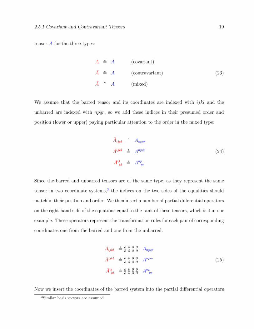
2.5.1 Covariant and Contravariant Tensors 19
tensor A for the three types:
A $ A (covariant)
A $ A (contravariant) (23)
A $ A (mixed)
We assume that the barred tensor and its coordinates are indexed with ijkl and the
unbarred are indexed with npqr, so we add these indices in their presumed order and
position (lower or upper) paying particular attention to the order in the mixed type:
Aijkl $ Anpqr
Aijkl $ Anpqr (24)
Aijkl $ Anpqr
Since the barred and unbarred tensors are of the same type, as they represent the same
tensor in two coordinate systems,3 the indices on the two sides of the equalities should
match in their position and order. We then insert a number of partial differential operators
on the right hand side of the equations equal to the rank of these tensors, which is 4 in our
example. These operators represent the transformation rules for each pair of corresponding
coordinates one from the barred and one from the unbarred:
Aijkl $ ∂∂∂∂∂∂∂∂
Anpqr
Aijkl $ ∂∂∂∂∂∂∂∂
Anpqr (25)
Aijkl $ ∂∂∂∂∂∂∂∂
Anpqr
Now we insert the coordinates of the barred system into the partial differential operators
3Similar basis vectors are assumed.
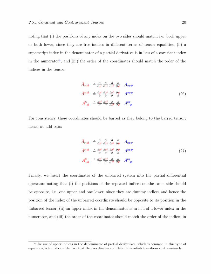
2.5.1 Covariant and Contravariant Tensors 20
noting that (i) the positions of any index on the two sides should match, i.e. both upper
or both lower, since they are free indices in different terms of tensor equalities, (ii) a
superscript index in the denominator of a partial derivative is in lieu of a covariant index
in the numerator4, and (iii) the order of the coordinates should match the order of the
indices in the tensor:
Aijkl $ ∂∂xi
∂∂xj
∂∂xk
∂∂xl
Anpqr
Aijkl $ ∂xi
∂∂xj
∂∂xk
∂∂xl
∂Anpqr (26)
Aijkl $ ∂xi
∂∂xj
∂∂∂xk
∂∂xl
Anpqr
For consistency, these coordinates should be barred as they belong to the barred tensor;
hence we add bars:
Aijkl $ ∂∂xi
∂∂xj
∂∂xk
∂∂xl
Anpqr
Aijkl $ ∂xi
∂∂xj
∂∂xk
∂∂xl
∂Anpqr (27)
Aijkl $ ∂xi
∂∂xj
∂∂∂xk
∂∂xl
Anpqr
Finally, we insert the coordinates of the unbarred system into the partial differential
operators noting that (i) the positions of the repeated indices on the same side should
be opposite, i.e. one upper and one lower, since they are dummy indices and hence the
position of the index of the unbarred coordinate should be opposite to its position in the
unbarred tensor, (ii) an upper index in the denominator is in lieu of a lower index in the
numerator, and (iii) the order of the coordinates should match the order of the indices in
4The use of upper indices in the denominator of partial derivatives, which is common in this type ofequations, is to indicate the fact that the coordinates and their differentials transform contravariantly.
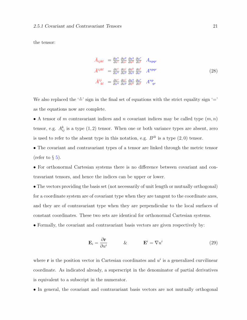
2.5.1 Covariant and Contravariant Tensors 21
the tensor:
Aijkl = ∂xn
∂xi∂xp
∂xj∂xq
∂xk∂xr
∂xlAnpqr
Aijkl = ∂xi
∂xn∂xj
∂xp∂xk
∂xq∂xl
∂xrAnpqr (28)
Aijkl = ∂xi
∂xn∂xj
∂xp∂xq
∂xk∂xr
∂xlAnpqr
We also replaced the ‘$’ sign in the final set of equations with the strict equality sign ‘=’
as the equations now are complete.
• A tensor of m contravariant indices and n covariant indices may be called type (m,n)
tensor, e.g. Akij is a type (1, 2) tensor. When one or both variance types are absent, zero
is used to refer to the absent type in this notation, e.g. Bik is a type (2, 0) tensor.
• The covariant and contravariant types of a tensor are linked through the metric tensor
(refer to § 5).
• For orthonormal Cartesian systems there is no difference between covariant and con-
travariant tensors, and hence the indices can be upper or lower.
• The vectors providing the basis set (not necessarily of unit length or mutually orthogonal)
for a coordinate system are of covariant type when they are tangent to the coordinate axes,
and they are of contravariant type when they are perpendicular to the local surfaces of
constant coordinates. These two sets are identical for orthonormal Cartesian systems.
• Formally, the covariant and contravariant basis vectors are given respectively by:
Ei =∂r
∂ui& Ei = ∇ui (29)
where r is the position vector in Cartesian coordinates and ui is a generalized curvilinear
coordinate. As indicated already, a superscript in the denominator of partial derivatives
is equivalent to a subscript in the numerator.
• In general, the covariant and contravariant basis vectors are not mutually orthogonal
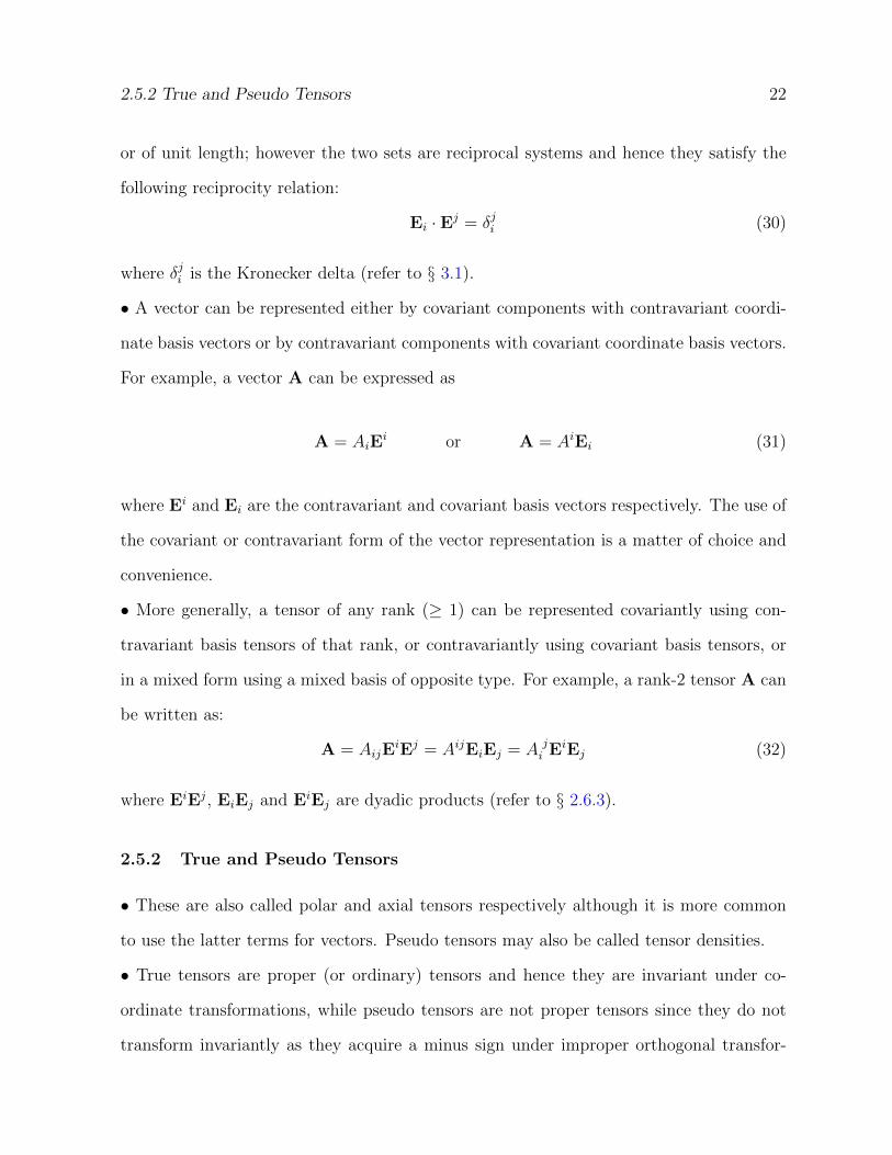
2.5.2 True and Pseudo Tensors 22
or of unit length; however the two sets are reciprocal systems and hence they satisfy the
following reciprocity relation:
Ei · Ej = δji (30)
where δji is the Kronecker delta (refer to § 3.1).
• A vector can be represented either by covariant components with contravariant coordi-
nate basis vectors or by contravariant components with covariant coordinate basis vectors.
For example, a vector A can be expressed as
A = AiEi or A = AiEi (31)
where Ei and Ei are the contravariant and covariant basis vectors respectively. The use of
the covariant or contravariant form of the vector representation is a matter of choice and
convenience.
• More generally, a tensor of any rank (≥ 1) can be represented covariantly using con-
travariant basis tensors of that rank, or contravariantly using covariant basis tensors, or
in a mixed form using a mixed basis of opposite type. For example, a rank-2 tensor A can
be written as:
A = AijEiEj = AijEiEj = A j
i EiEj (32)
where EiEj, EiEj and EiEj are dyadic products (refer to § 2.6.3).
2.5.2 True and Pseudo Tensors
• These are also called polar and axial tensors respectively although it is more common
to use the latter terms for vectors. Pseudo tensors may also be called tensor densities.
• True tensors are proper (or ordinary) tensors and hence they are invariant under co-
ordinate transformations, while pseudo tensors are not proper tensors since they do not
transform invariantly as they acquire a minus sign under improper orthogonal transfor-
2.5.2 True and Pseudo Tensors 23
mations which involve inversion of coordinate axes through the origin with a change of
system handedness.
• Because true and pseudo tensors have different mathematical properties and represent
different types of physical entities, the terms of consistent tensor expressions and equations
should be uniform in their true and pseudo type, i.e. all terms are true or all are pseudo.
• The direct product (refer to § 2.6.3) of even number of pseudo tensors is a proper tensor,
while the direct product of odd number of pseudo tensors is a pseudo tensor. The direct
product of true tensors is obviously a true tensor.
• The direct product of a mix of true and pseudo tensors is a true or pseudo tensor
depending on the number of pseudo tensors involved in the product as being even or odd
respectively.
• Similar rules to those of direct product apply to cross products (including curl operations)
involving tensors (usually of rank-1) with the addition of a pseudo factor for each cross
product operation. This factor is contributed by the permutation tensor (see § 3.2) which
is implicit in the definition of the cross product (see Eqs. 121 and 146).
• In summary, what determines the tensor type (true or pseudo) of the tensor terms in-
volving direct5 and cross products is the parity of the multiplicative factors of pseudo type
plus the number of cross product operations involved since each cross product contributes
an ε factor.
• Examples of true scalars are temperature, mass and the dot product of two polar or two
axial vectors, while examples of pseudo scalars are the dot product of an axial vector and
a polar vector and the scalar triple product of polar vectors.
• Examples of polar vectors are displacement and acceleration, while examples of axial
vectors are angular velocity and cross product of polar vectors in general (including curl
operation on polar vectors) due to the involvement of the permutation symbol which is
5Inner product (see § 2.6.5) is the result of a direct product operation followed by a contraction (see§ 2.6.4) and hence it is a direct product in this context.
2.5.3 Absolute and Relative Tensors 24
a pseudo tensor (refer to § 3.2). The essence of this distinction is that the direction of a
pseudo vector depends on the observer choice of the handedness of the coordinate system
whereas the direction of a proper vector is independent of such choice.
• Examples of proper tensors of rank-2 are stress and rate of strain tensors, while examples
of pseudo tensors of rank-2 are direct products of two vectors: one polar and one axial.
• Examples of proper tensors of higher ranks are piezoelectric moduli tensor (rank-3)
and elasticity tensor (rank-4), while examples of pseudo tensors of higher ranks are the
permutation tensor of these ranks.
2.5.3 Absolute and Relative Tensors
• Considering an arbitrary transformation from a general coordinate system to another, a
relative tensor of weight w is defined by the following tensor transformation:
Aij...klm...n =
∣∣∣∣∂x∂x∣∣∣∣w ∂xi∂xa
∂xj
∂xb· · · ∂x
k
∂xc∂xd
∂xl∂xe
∂xm· · · ∂x
f
∂xnAab...cde...f (33)
where∣∣∂x∂x
∣∣ is the Jacobian of the transformation between the two systems. When w = 0
the tensor is described as an absolute or true tensor, while when w = −1 the tensor is
described as a pseudo tensor. When w = 1 the tensor may be described as a tensor
density.6
• As indicated earlier, a tensor of m contravariant indices and n covariant indices may be
called type (m,n). This may be generalized to include the weight as a third entry and
hence the type of the tensor is identified by (m,n,w).
• Relative tensors can be added and subtracted if they are of the same variance type and
have the same weight; the result is a tensor of the same type and weight. Also, relative
tensors can be equated if they are of the same type and weight.
• Multiplication of relative tensors produces a relative tensor whose weight is the sum of
6Some of these labels are used differently by different authors.
2.5.4 Isotropic and Anisotropic Tensors 25
the weights of the original tensors. Hence, if the weights are added up to a non-zero value
the result is a relative tensor of that weight; otherwise it is an absolute tensor.
2.5.4 Isotropic and Anisotropic Tensors
• Isotropic tensors are characterized by the property that the values of their components
are invariant under coordinate transformation by proper rotation of axes. In contrast, the
values of the components of anisotropic tensors are dependent on the orientation of the
coordinate axes. Notable examples of isotropic tensors are scalars (rank-0), the vector 0
(rank-1), Kronecker delta δij (rank-2) and Levi-Civita tensor εijk (rank-3). Many tensors
describing physical properties of materials, such as stress and magnetic susceptibility, are
anisotropic.
• Direct and inner products of isotropic tensors are isotropic tensors.
• The zero tensor of any rank is isotropic; therefore if the components of a tensor vanish
in a particular coordinate system they will vanish in all properly and improperly rotated
coordinate systems.7 Consequently, if the components of two tensors are identical in a
particular coordinate system they are identical in all transformed coordinate systems.
• As indicated, all rank-0 tensors (scalars) are isotropic. Also, the zero vector, 0, of any
dimension is isotropic; in fact it is the only rank-1 isotropic tensor.
2.5.5 Symmetric and Anti-symmetric Tensors
• These types of tensor apply to high ranks only (rank ≥ 2). Moreover, these types are
not exhaustive, even for tensors of ranks ≥ 2, as there are high-rank tensors which are
neither symmetric nor anti-symmetric.
7For improper rotation, this is more general than being isotropic.
2.5.5 Symmetric and Anti-symmetric Tensors 26
• A rank-2 tensor Aij is symmetric iff for all i and j
Aji = Aij (34)
and anti-symmetric or skew-symmetric iff
Aji = −Aij (35)
Similar conditions apply to contravariant type tensors (refer also to the following).
• A rank-n tensor Ai1...in is symmetric in its two indices ij and il iff
Ai1...il...ij ...in = Ai1...ij ...il...in (36)
and anti-symmetric or skew-symmetric in its two indices ij and il iff
Ai1...il...ij ...in = −Ai1...ij ...il...in (37)
• Any rank-2 tensor Aij can be synthesized from (or decomposed into) a symmetric part
A(ij) (marked with round brackets enclosing the indices) and an anti-symmetric part A[ij]
(marked with square brackets) where
Aij = A(ij) + A[ij], A(ij) =1
2(Aij + Aji) & A[ij] =
1
2(Aij − Aji) (38)
• A rank-3 tensor Aijk can be symmetrized by
A(ijk) =1
3!(Aijk + Akij + Ajki + Aikj + Ajik + Akji) (39)
2.5.5 Symmetric and Anti-symmetric Tensors 27
and anti-symmetrized by
A[ijk] =1
3!(Aijk + Akij + Ajki − Aikj − Ajik − Akji) (40)
• A rank-n tensor Ai1...in can be symmetrized by
A(i1...in) =1
n!(sum of all even & odd permutations of indices i’s) (41)
and anti-symmetrized by
A[i1...in] =1
n!(sum of all even permutations minus sum of all odd permutations) (42)
• For a symmetric tensor Aij and an anti-symmetric tensor Bij (or the other way around)
we have
AijBij = 0 (43)
• The indices whose exchange defines the symmetry and anti-symmetry relations should
be of the same variance type, i.e. both upper or both lower.
• The symmetry and anti-symmetry characteristic of a tensor is invariant under coordinate
transformation.
• A tensor of high rank (> 2) may be symmetrized or anti-symmetrized with respect to
only some of its indices instead of all of its indices, e.g.
A(ij)k =1
2(Aijk + Ajik) & A[ij]k =
1
2(Aijk − Ajik) (44)
• A tensor is totally symmetric iff
Ai1...in = A(i1...in) (45)
2.6 Tensor Operations 28
and totally anti-symmetric iff
Ai1...in = A[i1...in] (46)
• For a totally skew-symmetric tensor (i.e. anti-symmetric in all of its indices), nonzero
entries can occur only when all the indices are different.
2.6 Tensor Operations
• There are many operations that can be performed on tensors to produce other tensors
in general. Some examples of these operations are addition/subtraction, multiplication
by a scalar (rank-0 tensor), multiplication of tensors (each of rank > 0), contraction and
permutation. Some of these operations, such as addition and multiplication, involve more
than one tensor while others are performed on a single tensor, such as contraction and
permutation.
• In tensor algebra, division is allowed only for scalars, hence if the components of an
indexed tensor should appear in a denominator, the tensor should be redefined to avoid
this, e.g. Bi = 1Ai
.
2.6.1 Addition and Subtraction
• Tensors of the same rank and type (covariant/contravariant/mixed and true/pseudo)
can be added algebraically to produce a tensor of the same rank and type, e.g.
a = b+ c (47)
Ai = Bi − Ci (48)
2.6.2 Multiplication by Scalar 29
Aij = Bij + Ci
j (49)
• The added/subtracted terms should have the same indicial structure with regard to
their free indices, as explained in § 2.2, hence Aijk and Bjik cannot be added or subtracted
although they are of the same rank and type, but Amimjk and Bijk can be added and sub-
tracted.
• Addition of tensors is associative and commutative:
(A + B) + C = A + (B + C) (50)
A + B = B + A (51)
2.6.2 Multiplication by Scalar
• A tensor can be multiplied by a scalar, which generally should not be zero, to produce
a tensor of the same variance type and rank, e.g.
Ajik = aBjik (52)
where a is a non-zero scalar.
• As indicated above, multiplying a tensor by a scalar means multiplying each component
of the tensor by that scalar.
• Multiplication by a scalar is commutative, and associative when more than two factors
are involved.
2.6.3 Tensor Multiplication 30
2.6.3 Tensor Multiplication
• This may also be called outer or exterior or direct or dyadic multiplication, although
some of these names may be reserved for operations on vectors.
• On multiplying each component of a tensor of rank r by each component of a tensor of
rank k, both of dimension m, a tensor of rank (r + k) with mr+k components is obtained
where the variance type of each index (covariant or contravariant) is preserved, e.g.
AiBj = Cij (53)
AijBkl = Cijkl (54)
• The outer product of a tensor of type (m,n) by a tensor of type (p, q) results in a tensor
of type (m+ p, n+ q).
• Direct multiplication of tensors may be marked by the symbol �, mostly when using
symbolic notation for tensors, e.g. A � B. However, in the present text no symbol will be
used for the operation of direct multiplication.
• Direct multiplication of tensors is not commutative.
• The outer product operation is distributive with respect to the algebraic sum of tensors:
A (B±C) = AB±AC & (B±C) A = BA±CA (55)
• Multiplication of a tensor by a scalar (refer to § 2.6.2) may be regarded as a special case
of direct multiplication.
• The rank-2 tensor constructed as a result of the direct multiplication of two vectors is
commonly called dyad.
• Tensors may be expressed as an outer product of vectors where the rank of the resultant
2.6.4 Contraction 31
product is equal to the number of the vectors involved (e.g. 2 for dyads and 3 for triads).
• Not every tensor can be synthesized as a product of lower rank tensors.
• In the outer product, it is understood that all the indices of the involved tensors have
the same range.
• The outer product of tensors yields a tensor.
2.6.4 Contraction
• Contraction of a tensor of rank > 1 is to make two free indices identical, by unifying
their symbols, and perform summation over these repeated indices, e.g.
Aji contraction−−−−−−−−→ Aii (56)
Ajkil contraction on jl−−−−−−−−−−−−→ Amkim (57)
• Contraction results in a reduction of the rank by 2 since it implies the annihilation of
two free indices. Therefore, the contraction of a rank-2 tensor is a scalar, the contraction
of a rank-3 tensor is a vector, the contraction of a rank-4 tensor is a rank-2 tensor, and so
on.
• For general non-Cartesian coordinate systems, the pair of contracted indices should be
different in their variance type, i.e. one upper and one lower. Hence, contraction of a
mixed tensor of type (m,n) will, in general, produce a tensor of type (m− 1, n− 1).
• A tensor of type (p, q) can have p× q possible contractions, i.e. one contraction for each
pair of lower and upper indices.
• A common example of contraction is the dot product operation on vectors which can be
regarded as a direct multiplication (refer to § 2.6.3) of the two vectors, which results in a
rank-2 tensor, followed by a contraction.

2.6.5 Inner Product 32
• In matrix algebra, taking the trace (summing the diagonal elements) can also be consid-
ered as contraction of the matrix, which under certain conditions can represent a rank-2
tensor, and hence it yields the trace which is a scalar.
• Applying the index contraction operation on a tensor results into a tensor.
• Application of contraction of indices operation on a relative tensor (see § 2.5.3) produces
a relative tensor of the same weight as the original tensor.
2.6.5 Inner Product
• On taking the outer product (refer to § 2.6.3) of two tensors of rank ≥ 1 followed by a
contraction on two indices of the product, an inner product of the two tensors is formed.
Hence if one of the original tensors is of rank-m and the other is of rank-n, the inner
product will be of rank-(m+ n− 2).
• The inner product operation is usually symbolized by a single dot between the two
tensors, e.g. A ·B, to indicate contraction following outer multiplication.
• In general, the inner product is not commutative. When one or both of the tensors
involved in the inner product are of rank > 1 the order of the multiplicands does matter.
• The inner product operation is distributive with respect to the algebraic sum of tensors:
A · (B±C) = A ·B±A ·C & (B±C) ·A = B ·A±C ·A (58)
• As indicated before (see § 2.6.4), the dot product of two vectors is an example of the
inner product of tensors, i.e. it is an inner product of two rank-1 tensors to produce a
rank-0 tensor:
[ab] ji = aibj contraction−−−−−−−−→ a · b = aib
i (59)
• Another common example (from linear algebra) of inner product is the multiplication of
a matrix (representing a rank-2 tensor assuming certain conditions) by a vector (rank-1
2.6.5 Inner Product 33
tensor) to produce a vector, e.g.
[Ab] kij = Aijbk contraction on jk−−−−−−−−−−−−−→ [A · b]i = Aijb
j (60)
The multiplication of two n × n matrices is another example of inner product (see Eq.
119).
• For tensors whose outer product produces a tensor of rank > 2, various contraction
operations between different sets of indices can occur and hence more than one inner
product, which are different in general, can be defined. Moreover, when the outer product
produces a tensor of rank > 3 more than one contraction can take place simultaneously.
• There are more specialized types of inner product; some of which may be defined dif-
ferently by different authors. For example, a double inner product of two rank-2 tensors,
A and B, may be defined and denoted by double vertically- or horizontally-aligned dots
(e.g. A : B or A · ·B) to indicate double contraction taking place between different pairs
of indices. An instance of these types is the inner product with double contraction of two
dyads which is commonly defined by8
ab : cd = (a · c) (b · d) (61)
and the result is a scalar. The single dots in the right hand side of the last equation
symbolize the conventional dot product of two vectors. Some authors may define a different
type of double-contraction inner product of two dyads, symbolized by two horizontally-
aligned dots, which may be called a “transposed contraction”, and is given by
ab · ·cd = ab : dc = (a · d) (b · c) (62)
8It is also defined differently by some authors.
2.6.6 Permutation 34
where the result is also a scalar. However, different authors may have different conventions
and hence one should be vigilant about such differences.
• For two rank-2 tensors, the aforementioned double-contraction inner products are simi-
larly defined as in the case of two dyads:
A : B = AijBij & A · ·B = AijBji (63)
• Inner products with higher multiplicity of contractions are similarly defined, and hence
can be regarded as trivial extensions of the inner products with lower contraction multi-
plicities.
• The inner product of tensors produces a tensor because the inner product is an outer
product operation followed by an index contraction operation and both of these operations
on tensors produce tensors.
2.6.6 Permutation
• A tensor may be obtained by exchanging the indices of another tensor, e.g. transposition
of rank-2 tensors.
• Tensor permutation applies only to tensors of rank ≥ 2.
• The collection of tensors obtained by permuting the indices of a basic tensor may be
called isomers.
2.7 Tensor Test: Quotient Rule
• Sometimes a tensor-like object may be suspected for being a tensor; in such cases a test
based on the “quotient rule” can be used to clarify the situation. According to this rule, if
the inner product of a suspected tensor with a known tensor is a tensor then the suspect
is a tensor. In more formal terms, if it is not known if A is a tensor but it is known that
2.7 Tensor Test: Quotient Rule 35
B and C are tensors; moreover it is known that the following relation holds true in all
rotated (properly-transformed) coordinate frames:
Apq...k...mBij...k...n = Cpq...mij...n (64)
then A is a tensor. Here, A, B and C are respectively of ranks m, n and (m+n− 2), due
to the contraction on k which can be any index of A and B independently.
• Testing for being a tensor can also be done by applying first principles through direct
substitution in the transformation equations. However, using the quotient rule is generally
more convenient and requires less work.
• The quotient rule may be considered as a replacement for the division operation which
is not defined for tensors.
3 δ AND ε TENSORS 36
3 δ and ε Tensors
• These tensors are of particular importance in tensor calculus due to their distinctive
properties and unique transformation attributes. They are numerical tensors with fixed
components in all coordinate systems. The first is called Kronecker delta or unit ten-
sor, while the second is called Levi-Civita9, permutation, anti-symmetric and alternating
tensor.
• The δ and ε tensors are conserved under coordinate transformations and hence they are
the same for all systems of coordinate.10
3.1 Kronecker δ
• This is a rank-2 symmetric tensor in all dimensions, i.e.
δij = δji (i, j = 1, 2, . . . , n) (65)
Similar identities apply to the contravariant and mixed types of this tensor.
• It is invariant in all coordinate systems, and hence it is an isotropic tensor.11
• It is defined as:
δij =
1 (i = j)
0 (i 6= j)
(66)
9This name is usually used for the rank-3 tensor. Also some authors distinguish between the permuta-tion tensor and Levi-Civita tensor even for rank-3. Moreover, some of the common labels and descriptionsof ε are more specific to rank-3.
10For the permutation tensor, the statement applies to proper coordinate transformations.11In fact it is more general than isotropic as it is invariant even under improper coordinate transfor-
mations.
3.2 Permutation ε 37
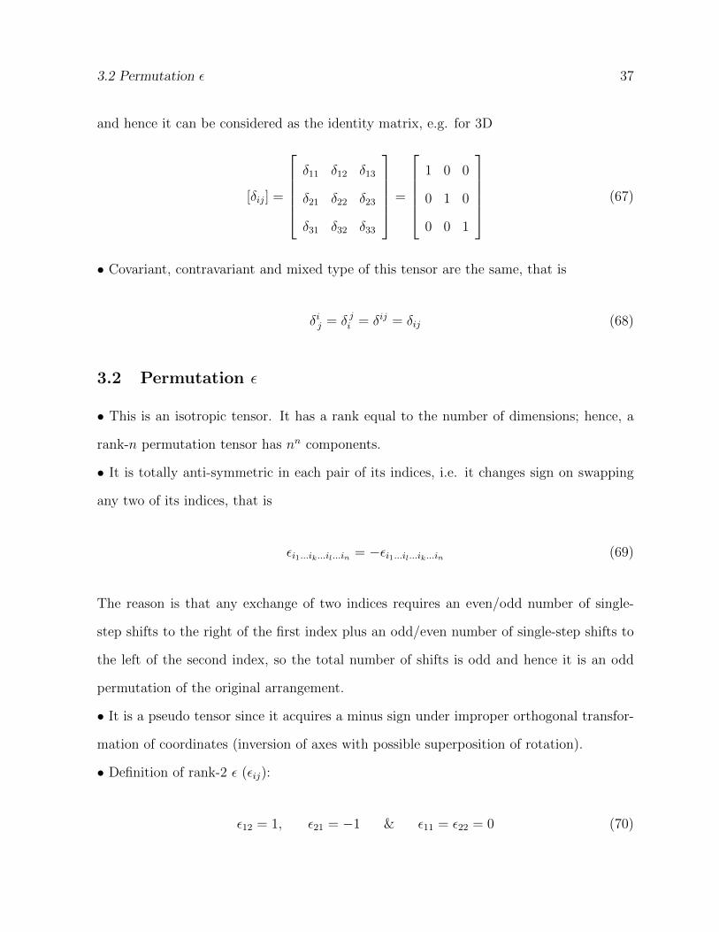
and hence it can be considered as the identity matrix, e.g. for 3D
[δij] =
δ11 δ12 δ13
δ21 δ22 δ23
δ31 δ32 δ33
=
1 0 0
0 1 0
0 0 1
(67)
• Covariant, contravariant and mixed type of this tensor are the same, that is
δij = δ ji = δij = δij (68)
3.2 Permutation ε
• This is an isotropic tensor. It has a rank equal to the number of dimensions; hence, a
rank-n permutation tensor has nn components.
• It is totally anti-symmetric in each pair of its indices, i.e. it changes sign on swapping
any two of its indices, that is
εi1...ik...il...in = −εi1...il...ik...in (69)
The reason is that any exchange of two indices requires an even/odd number of single-
step shifts to the right of the first index plus an odd/even number of single-step shifts to
the left of the second index, so the total number of shifts is odd and hence it is an odd
permutation of the original arrangement.
• It is a pseudo tensor since it acquires a minus sign under improper orthogonal transfor-
mation of coordinates (inversion of axes with possible superposition of rotation).
• Definition of rank-2 ε (εij):
ε12 = 1, ε21 = −1 & ε11 = ε22 = 0 (70)
3.3 Useful Identities Involving δ or/and ε 38
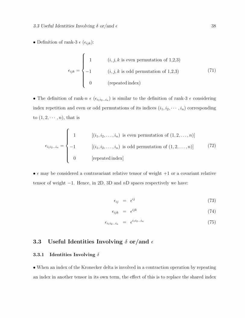
• Definition of rank-3 ε (εijk):
εijk =
1 (i, j, k is even permutation of 1,2,3)
−1 (i, j, k is odd permutation of 1,2,3)
0 (repeated index)
(71)
• The definition of rank-n ε (εi1i2...in) is similar to the definition of rank-3 ε considering
index repetition and even or odd permutations of its indices (i1, i2, · · · , in) corresponding
to (1, 2, · · · , n), that is
εi1i2...in =
1 [(i1, i2, . . . , in) is even permutation of (1, 2, . . . , n)]
−1 [(i1, i2, . . . , in) is odd permutation of (1, 2, . . . , n)]
0 [repeated index]
(72)
• ε may be considered a contravariant relative tensor of weight +1 or a covariant relative
tensor of weight −1. Hence, in 2D, 3D and nD spaces respectively we have:
εij = εij (73)
εijk = εijk (74)
εi1i2...in = εi1i2...in (75)
3.3 Useful Identities Involving δ or/and ε
3.3.1 Identities Involving δ
•When an index of the Kronecker delta is involved in a contraction operation by repeating
an index in another tensor in its own term, the effect of this is to replace the shared index
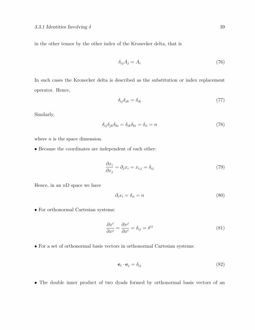
3.3.1 Identities Involving δ 39
in the other tensor by the other index of the Kronecker delta, that is
δijAj = Ai (76)
In such cases the Kronecker delta is described as the substitution or index replacement
operator. Hence,
δijδjk = δik (77)
Similarly,
δijδjkδki = δikδki = δii = n (78)
where n is the space dimension.
• Because the coordinates are independent of each other:
∂xi∂xj
= ∂jxi = xi,j = δij (79)
Hence, in an nD space we have
∂ixi = δii = n (80)
• For orthonormal Cartesian systems:
∂xi
∂xj=∂xj
∂xi= δij = δij (81)
• For a set of orthonormal basis vectors in orthonormal Cartesian systems:
ei · ej = δij (82)
• The double inner product of two dyads formed by orthonormal basis vectors of an
3.3.2 Identities Involving ε 40
orthonormal Cartesian system is given by:
eiej : ekel = δikδjl (83)
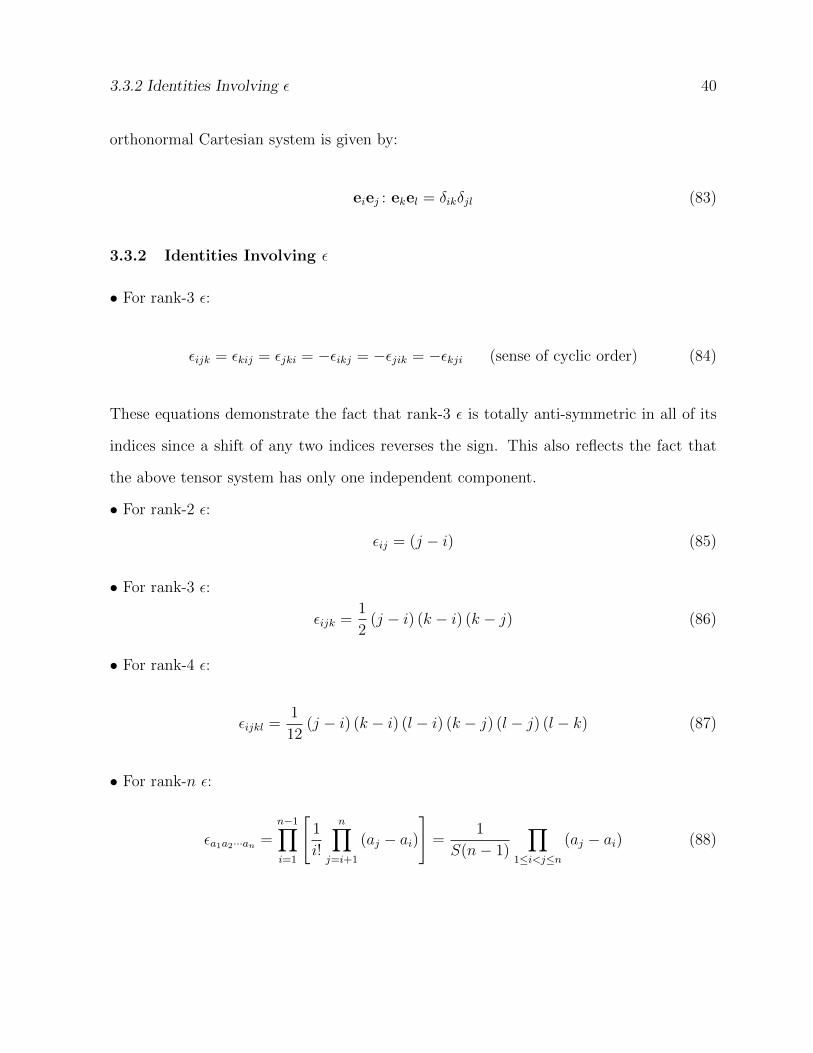
3.3.2 Identities Involving ε
• For rank-3 ε:
εijk = εkij = εjki = −εikj = −εjik = −εkji (sense of cyclic order) (84)
These equations demonstrate the fact that rank-3 ε is totally anti-symmetric in all of its
indices since a shift of any two indices reverses the sign. This also reflects the fact that
the above tensor system has only one independent component.
• For rank-2 ε:
εij = (j − i) (85)
• For rank-3 ε:
εijk =1
2(j − i) (k − i) (k − j) (86)
• For rank-4 ε:
εijkl =1
12(j − i) (k − i) (l − i) (k − j) (l − j) (l − k) (87)
• For rank-n ε:
εa1a2···an =n−1∏i=1
[1
i!
n∏j=i+1
(aj − ai)
]=
1
S(n− 1)
∏1≤i<j≤n
(aj − ai) (88)
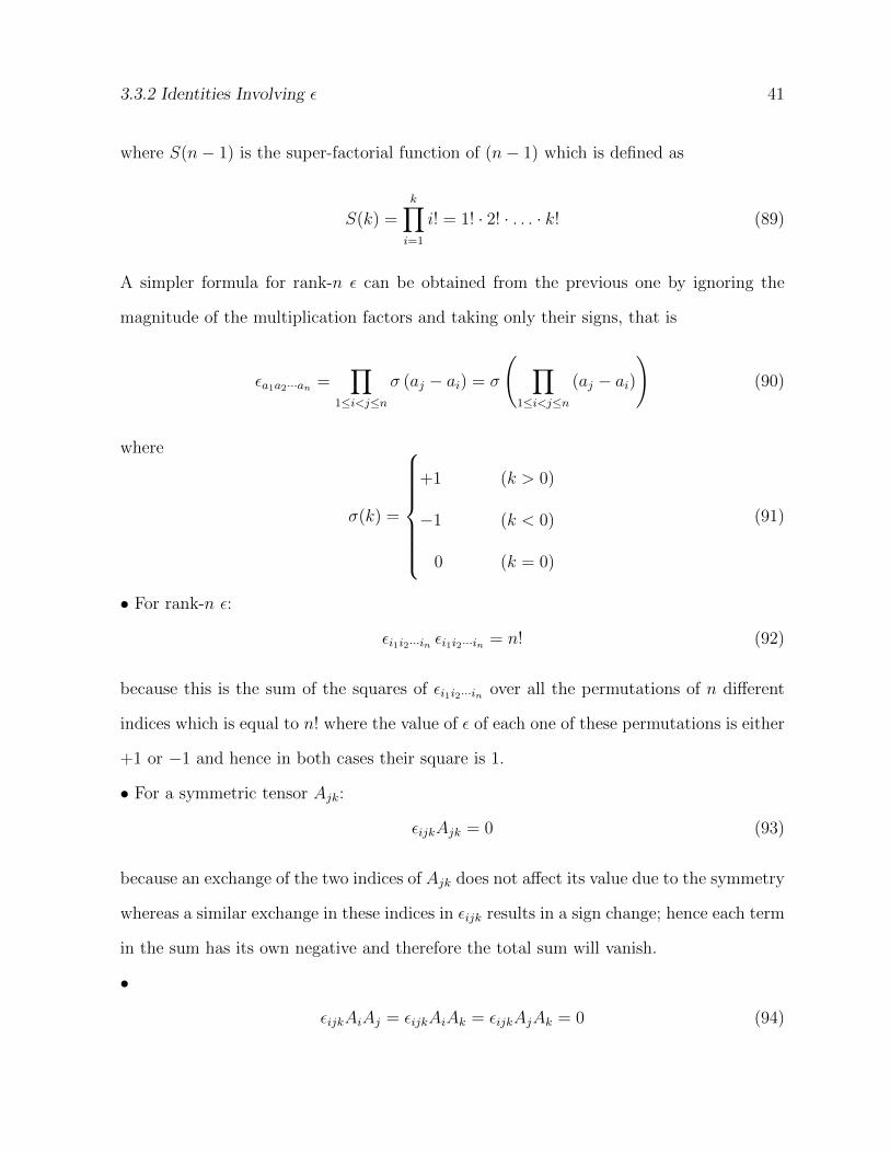
3.3.2 Identities Involving ε 41
where S(n− 1) is the super-factorial function of (n− 1) which is defined as
S(k) =k∏i=1
i! = 1! · 2! · . . . · k! (89)
A simpler formula for rank-n ε can be obtained from the previous one by ignoring the
magnitude of the multiplication factors and taking only their signs, that is
εa1a2···an =∏
1≤i<j≤n
σ (aj − ai) = σ
( ∏1≤i<j≤n
(aj − ai)
)(90)
where
σ(k) =
+1 (k > 0)
−1 (k < 0)
0 (k = 0)
(91)
• For rank-n ε:
εi1i2···in εi1i2···in = n! (92)
because this is the sum of the squares of εi1i2···in over all the permutations of n different
indices which is equal to n! where the value of ε of each one of these permutations is either
+1 or −1 and hence in both cases their square is 1.
• For a symmetric tensor Ajk:
εijkAjk = 0 (93)
because an exchange of the two indices of Ajk does not affect its value due to the symmetry
whereas a similar exchange in these indices in εijk results in a sign change; hence each term
in the sum has its own negative and therefore the total sum will vanish.
•
εijkAiAj = εijkAiAk = εijkAjAk = 0 (94)

3.3.3 Identities Involving δ and ε 42
because, due to the commutativity of multiplication, an exchange of the indices in A’s will
not affect the value but a similar exchange in the corresponding indices of εijk will cause
a change in sign; hence each term in the sum has its own negative and therefore the total
sum will be zero.
• For a set of orthonormal basis vectors in a 3D space with a right-handed orthonormal
Cartesian coordinate system:
ei × ej = εijkek (95)
ei · (ej × ek) = εijk (96)
3.3.3 Identities Involving δ and ε
•
εijkδ1iδ2jδ3k = ε123 = 1 (97)
• For rank-2 ε:
εijεkl =
∣∣∣∣∣∣∣δik δil
δjk δjl
∣∣∣∣∣∣∣ = δikδjl − δilδjk (98)
εilεkl = δik (99)
εijεij = 2 (100)
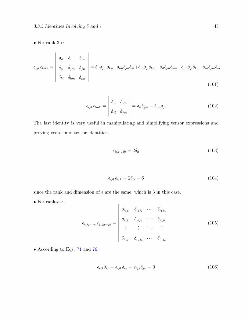
3.3.3 Identities Involving δ and ε 43
• For rank-3 ε:
εijkεlmn =
∣∣∣∣∣∣∣∣∣∣δil δim δin
δjl δjm δjn
δkl δkm δkn
∣∣∣∣∣∣∣∣∣∣= δilδjmδkn+δimδjnδkl+δinδjlδkm−δilδjnδkm−δimδjlδkn−δinδjmδkl
(101)
εijkεlmk =
∣∣∣∣∣∣∣δil δim
δjl δjm
∣∣∣∣∣∣∣ = δilδjm − δimδjl (102)
The last identity is very useful in manipulating and simplifying tensor expressions and
proving vector and tensor identities.
εijkεljk = 2δil (103)
εijkεijk = 2δii = 6 (104)
since the rank and dimension of ε are the same, which is 3 in this case.
• For rank-n ε:
εi1i2···in εj1j2···jn =
∣∣∣∣∣∣∣∣∣∣∣∣∣
δi1j1 δi1j2 · · · δi1jn
δi2j1 δi2j2 · · · δi2jn...
.... . .
...
δinj1 δinj2 · · · δinjn
∣∣∣∣∣∣∣∣∣∣∣∣∣(105)
• According to Eqs. 71 and 76:
εijkδij = εijkδik = εijkδjk = 0 (106)
3.4 Generalized Kronecker delta 44
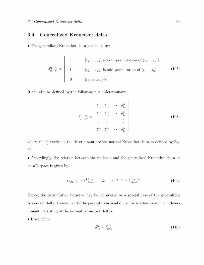
3.4 Generalized Kronecker delta
• The generalized Kronecker delta is defined by:
δi1...inj1...jn=
1 [(j1 . . . jn) is even permutation of (i1 . . . in)]
−1 [(j1 . . . jn) is odd permutation of (i1 . . . in)]
0 [repeated j’s]
(107)
It can also be defined by the following n× n determinant:
δi1...inj1...jn=
∣∣∣∣∣∣∣∣∣∣∣∣∣
δi1j1 δi1j2 · · · δi1jn
δi2j1 δi2j2 · · · δi2jn...
.... . .
...
δinj1 δinj2 · · · δinjn
∣∣∣∣∣∣∣∣∣∣∣∣∣(108)
where the δij entries in the determinant are the normal Kronecker delta as defined by Eq.
66.
• Accordingly, the relation between the rank-n ε and the generalized Kronecker delta in
an nD space is given by:
εi1i2...in = δ1 2...ni1i2...in
& εi1i2...in = δi1i2...in1 2...n (109)
Hence, the permutation tensor ε may be considered as a special case of the generalized
Kronecker delta. Consequently the permutation symbol can be written as an n× n deter-
minant consisting of the normal Kronecker deltas.
• If we define
δijlm = δijklmk (110)
3.4 Generalized Kronecker delta 45
then Eq. 102 will take the following form:
δijlm = δilδjm − δimδ
jl (111)
Other identities involving δ and ε can also be formulated in terms of the generalized
Kronecker delta.
• On comparing Eq. 105 with Eq. 108 we conclude
δi1...inj1...jn= εi1...in εj1...jn (112)
4 APPLICATIONS OF TENSOR NOTATION AND TECHNIQUES 46
4 Applications of Tensor Notation and Techniques
4.1 Common Definitions in Tensor Notation
• The trace of a matrix A representing a rank-2 tensor is:
tr (A) = Aii (113)
• For a 3× 3 matrix representing a rank-2 tensor in a 3D space, the determinant is:
det (A) =
∣∣∣∣∣∣∣∣∣∣A11 A12 A13
A21 A22 A23
A31 A32 A33
∣∣∣∣∣∣∣∣∣∣= εijkA1iA2jA3k = εijkAi1Aj2Ak3 (114)
where the last two equalities represent the expansion of the determinant by row and by
column. Alternatively
det (A) =1
3!εijkεlmnAilAjmAkn (115)
• For an n× n matrix representing a rank-2 tensor in an nD space, the determinant is:
det (A) = εi1···inA1i1 . . . Anin = εi1···inAi11 . . . Ainn =1
n!εi1···in εj1···jnAi1j1 . . . Ainjn (116)
• The inverse of a matrix A representing a rank-2 tensor is:
[A−1
]ij
=1
2 det (A)εjmn εipqAmpAnq (117)
• The multiplication of a matrix A by a vector b as defined in linear algebra is:
[Ab]i = Aijbj (118)
4.1 Common Definitions in Tensor Notation 47
It should be noticed that here we are using matrix notation. The multiplication operation,
according to the symbolic notation of tensors, should be denoted by a dot between the
tensor and the vector, i.e. A·b.12
• The multiplication of two n× n matrices A and B as defined in linear algebra is:
[AB]ik = AijBjk (119)
Again, here we are using matrix notation; otherwise a dot should be inserted between the
two matrices.
• The dot product of two vectors is:
A ·B =δijAiBj = AiBi (120)
The readers are referred to § 2.6.5 for a more general definition of this type of product
that includes higher rank tensors.
• The cross product of two vectors is:
[A×B]i = εijkAjBk (121)
• The scalar triple product of three vectors is:
A · (B×C) =
∣∣∣∣∣∣∣∣∣∣A1 A2 A3
B1 B2 B3
C1 C2 C3
∣∣∣∣∣∣∣∣∣∣= εijkAiBjCk (122)
12The matrix multiplication in matrix notation is equivalent to a dot product operation in tensornotation.
4.2 Scalar Invariants of Tensors 48
• The vector triple product of three vectors is:
[A× (B×C)]i = εijkεklmAjBlCm (123)
4.2 Scalar Invariants of Tensors
• In the following we list and write in tensor notation a number of invariants of low rank
tensors which have special importance due to their widespread applications in vector and
tensor calculus. All These invariants are scalars.
• The value of a scalar (rank-0 tensor), which consists of a magnitude and a sign, is
invariant under coordinate transformation.
• An invariant of a vector (rank-1 tensor) under coordinate transformations is its magni-
tude, i.e. length (the direction is also invariant but it is not scalar!).13
• The main three independent scalar invariants of a rank-2 tensor A under change of basis
are:
I = tr (A) = Aii (124)
II = tr(A2)
= AijAji (125)
III = tr(A3)
= AijAjkAki (126)
• Different forms of the three invariants of a rank-2 tensor A, which are also widely used,
are:
I1 = I = Aii (127)
13In fact the magnitude alone is invariant under coordinate transformations even for pseudo vectorsbecause it is a scalar.
4.3 Common Differential Operations in Tensor Notation 49
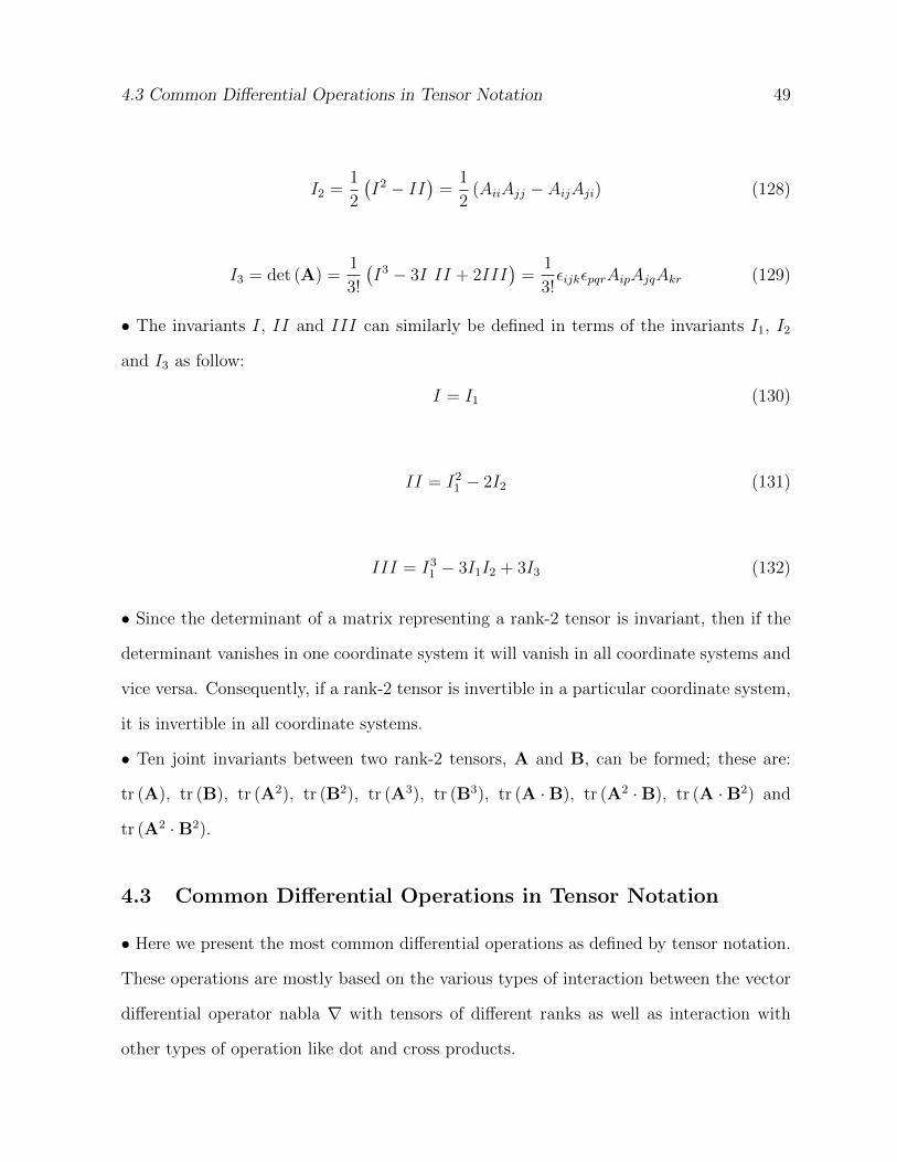
I2 =1
2
(I2 − II
)=
1
2(AiiAjj − AijAji) (128)
I3 = det (A) =1
3!
(I3 − 3I II + 2III
)=
1
3!εijkεpqrAipAjqAkr (129)
• The invariants I, II and III can similarly be defined in terms of the invariants I1, I2
and I3 as follow:
I = I1 (130)
II = I21 − 2I2 (131)
III = I31 − 3I1I2 + 3I3 (132)
• Since the determinant of a matrix representing a rank-2 tensor is invariant, then if the
determinant vanishes in one coordinate system it will vanish in all coordinate systems and
vice versa. Consequently, if a rank-2 tensor is invertible in a particular coordinate system,
it is invertible in all coordinate systems.
• Ten joint invariants between two rank-2 tensors, A and B, can be formed; these are:
tr (A), tr (B), tr (A2), tr (B2), tr (A3), tr (B3), tr (A ·B), tr (A2 ·B), tr (A ·B2) and
tr (A2 ·B2).
4.3 Common Differential Operations in Tensor Notation
• Here we present the most common differential operations as defined by tensor notation.
These operations are mostly based on the various types of interaction between the vector
differential operator nabla ∇ with tensors of different ranks as well as interaction with
other types of operation like dot and cross products.
4.3.1 Cartesian System 50
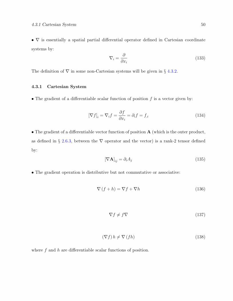
• ∇ is essentially a spatial partial differential operator defined in Cartesian coordinate
systems by:
∇i =∂
∂xi(133)
The definition of ∇ in some non-Cartesian systems will be given in § 4.3.2.
4.3.1 Cartesian System
• The gradient of a differentiable scalar function of position f is a vector given by:
[∇f ]i = ∇if =∂f
∂xi= ∂if = f,i (134)
• The gradient of a differentiable vector function of position A (which is the outer product,
as defined in § 2.6.3, between the ∇ operator and the vector) is a rank-2 tensor defined
by:
[∇A]ij = ∂iAj (135)
• The gradient operation is distributive but not commutative or associative:
∇ (f + h) = ∇f +∇h (136)
∇f 6= f∇ (137)
(∇f)h 6= ∇ (fh) (138)
where f and h are differentiable scalar functions of position.
4.3.1 Cartesian System 51
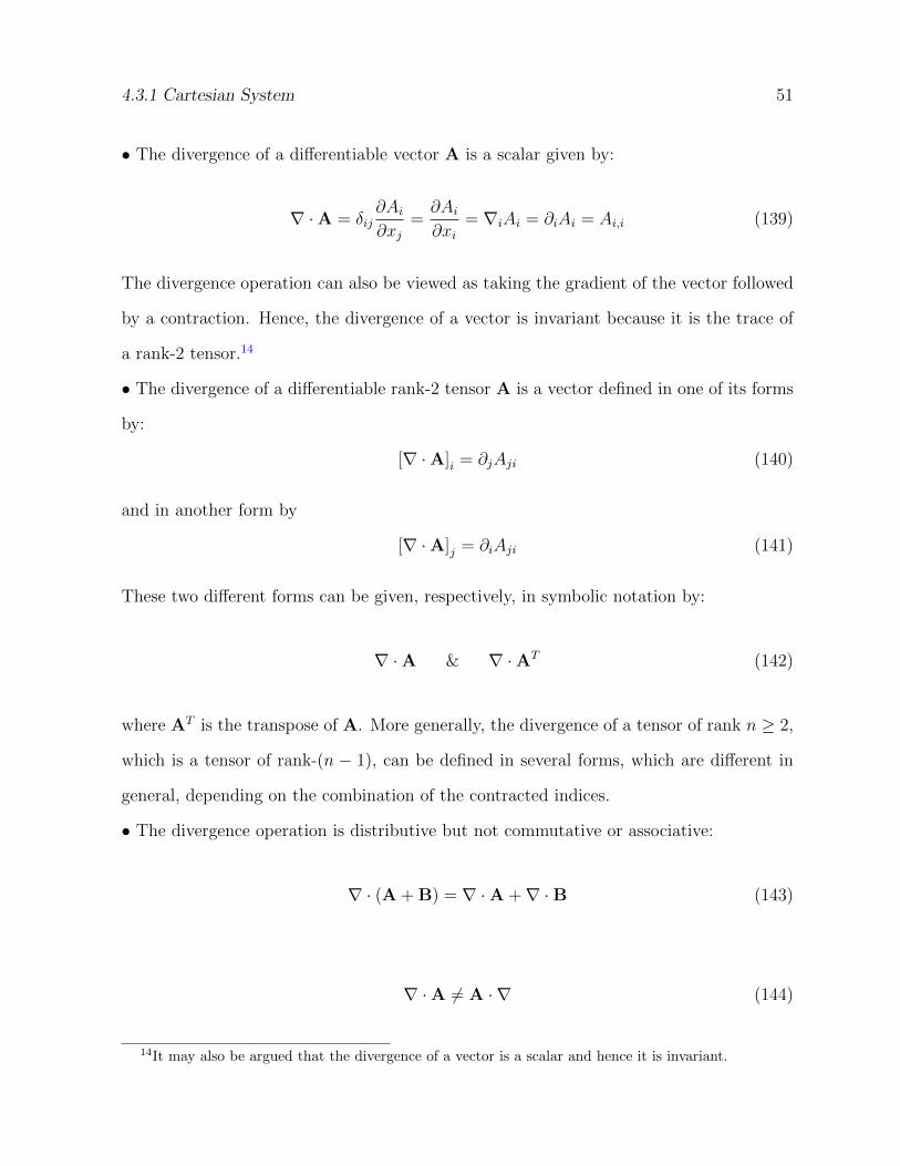
• The divergence of a differentiable vector A is a scalar given by:
∇ ·A = δij∂Ai∂xj
=∂Ai∂xi
= ∇iAi = ∂iAi = Ai,i (139)
The divergence operation can also be viewed as taking the gradient of the vector followed
by a contraction. Hence, the divergence of a vector is invariant because it is the trace of
a rank-2 tensor.14
• The divergence of a differentiable rank-2 tensor A is a vector defined in one of its forms
by:
[∇ ·A]i = ∂jAji (140)
and in another form by
[∇ ·A]j = ∂iAji (141)
These two different forms can be given, respectively, in symbolic notation by:
∇ ·A & ∇ ·AT (142)
where AT is the transpose of A. More generally, the divergence of a tensor of rank n ≥ 2,
which is a tensor of rank-(n − 1), can be defined in several forms, which are different in
general, depending on the combination of the contracted indices.
• The divergence operation is distributive but not commutative or associative:
∇ · (A + B) = ∇ ·A +∇ ·B (143)
∇ ·A 6= A · ∇ (144)
14It may also be argued that the divergence of a vector is a scalar and hence it is invariant.
4.3.1 Cartesian System 52
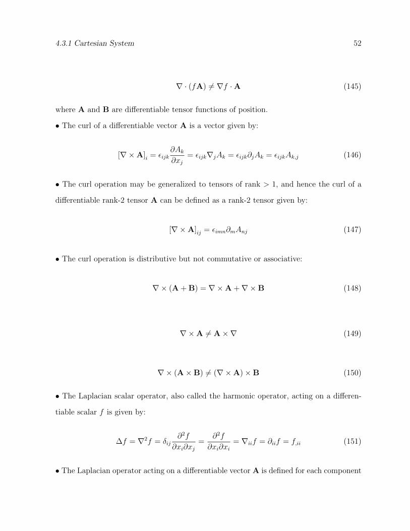
∇ · (fA) 6= ∇f ·A (145)
where A and B are differentiable tensor functions of position.
• The curl of a differentiable vector A is a vector given by:
[∇×A]i = εijk∂Ak∂xj
= εijk∇jAk = εijk∂jAk = εijkAk,j (146)
• The curl operation may be generalized to tensors of rank > 1, and hence the curl of a
differentiable rank-2 tensor A can be defined as a rank-2 tensor given by:
[∇×A]ij = εimn∂mAnj (147)
• The curl operation is distributive but not commutative or associative:
∇× (A + B) = ∇×A +∇×B (148)
∇×A 6= A×∇ (149)
∇× (A×B) 6= (∇×A)×B (150)
• The Laplacian scalar operator, also called the harmonic operator, acting on a differen-
tiable scalar f is given by:
∆f = ∇2f = δij∂2f
∂xi∂xj=
∂2f
∂xi∂xi= ∇iif = ∂iif = f,ii (151)
• The Laplacian operator acting on a differentiable vector A is defined for each component
4.3.2 Other Coordinate Systems 53
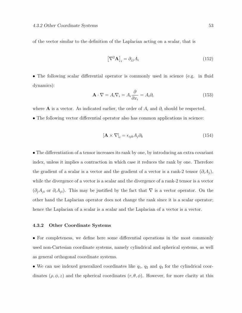
of the vector similar to the definition of the Laplacian acting on a scalar, that is
[∇2A
]i
= ∂jjAi (152)
• The following scalar differential operator is commonly used in science (e.g. in fluid
dynamics):
A · ∇ = Ai∇i = Ai∂
∂xi= Ai∂i (153)
where A is a vector. As indicated earlier, the order of Ai and ∂i should be respected.
• The following vector differential operator also has common applications in science:
[A×∇]i = εijkAj∂k (154)
• The differentiation of a tensor increases its rank by one, by introducing an extra covariant
index, unless it implies a contraction in which case it reduces the rank by one. Therefore
the gradient of a scalar is a vector and the gradient of a vector is a rank-2 tensor (∂iAj),
while the divergence of a vector is a scalar and the divergence of a rank-2 tensor is a vector
(∂jAji or ∂iAji). This may be justified by the fact that ∇ is a vector operator. On the
other hand the Laplacian operator does not change the rank since it is a scalar operator;
hence the Laplacian of a scalar is a scalar and the Laplacian of a vector is a vector.
4.3.2 Other Coordinate Systems
• For completeness, we define here some differential operations in the most commonly
used non-Cartesian coordinate systems, namely cylindrical and spherical systems, as well
as general orthogonal coordinate systems.
• We can use indexed generalized coordinates like q1, q2 and q3 for the cylindrical coor-
dinates (ρ, φ, z) and the spherical coordinates (r, θ, φ). However, for more clarity at this
4.3.2 Other Coordinate Systems 54
level and to follow the more conventional practice, we use the coordinates of these systems
as suffixes in place of the indices used in the tensor notation.15
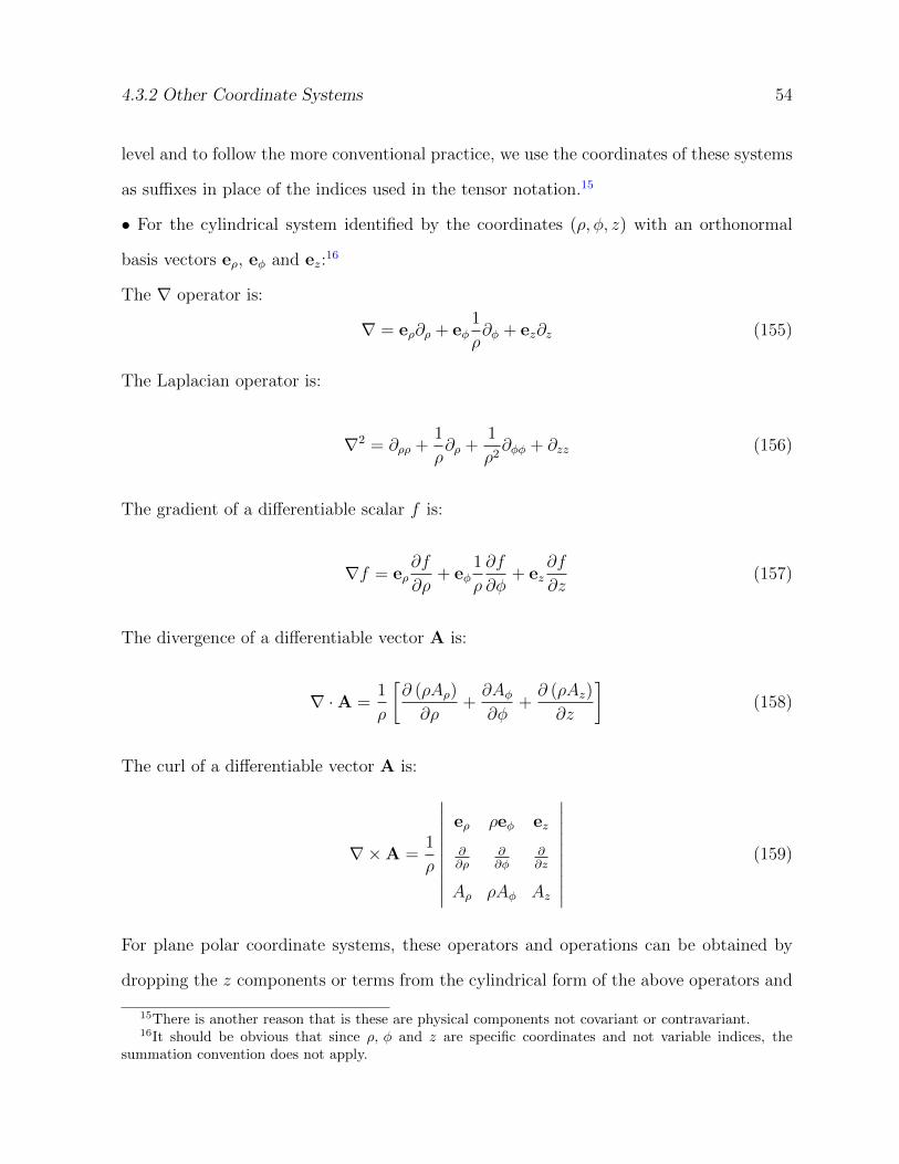
• For the cylindrical system identified by the coordinates (ρ, φ, z) with an orthonormal
basis vectors eρ, eφ and ez:16
The ∇ operator is:
∇ = eρ∂ρ + eφ1
ρ∂φ + ez∂z (155)
The Laplacian operator is:
∇2 = ∂ρρ +1
ρ∂ρ +
1
ρ2∂φφ + ∂zz (156)
The gradient of a differentiable scalar f is:
∇f = eρ∂f
∂ρ+ eφ
1
ρ
∂f
∂φ+ ez
∂f
∂z(157)
The divergence of a differentiable vector A is:
∇ ·A =1
ρ
[∂ (ρAρ)
∂ρ+∂Aφ∂φ
+∂ (ρAz)
∂z
](158)
The curl of a differentiable vector A is:
∇×A =1
ρ
∣∣∣∣∣∣∣∣∣∣eρ ρeφ ez
∂∂ρ
∂∂φ
∂∂z
Aρ ρAφ Az
∣∣∣∣∣∣∣∣∣∣(159)
For plane polar coordinate systems, these operators and operations can be obtained by
dropping the z components or terms from the cylindrical form of the above operators and
15There is another reason that is these are physical components not covariant or contravariant.16It should be obvious that since ρ, φ and z are specific coordinates and not variable indices, the
summation convention does not apply.
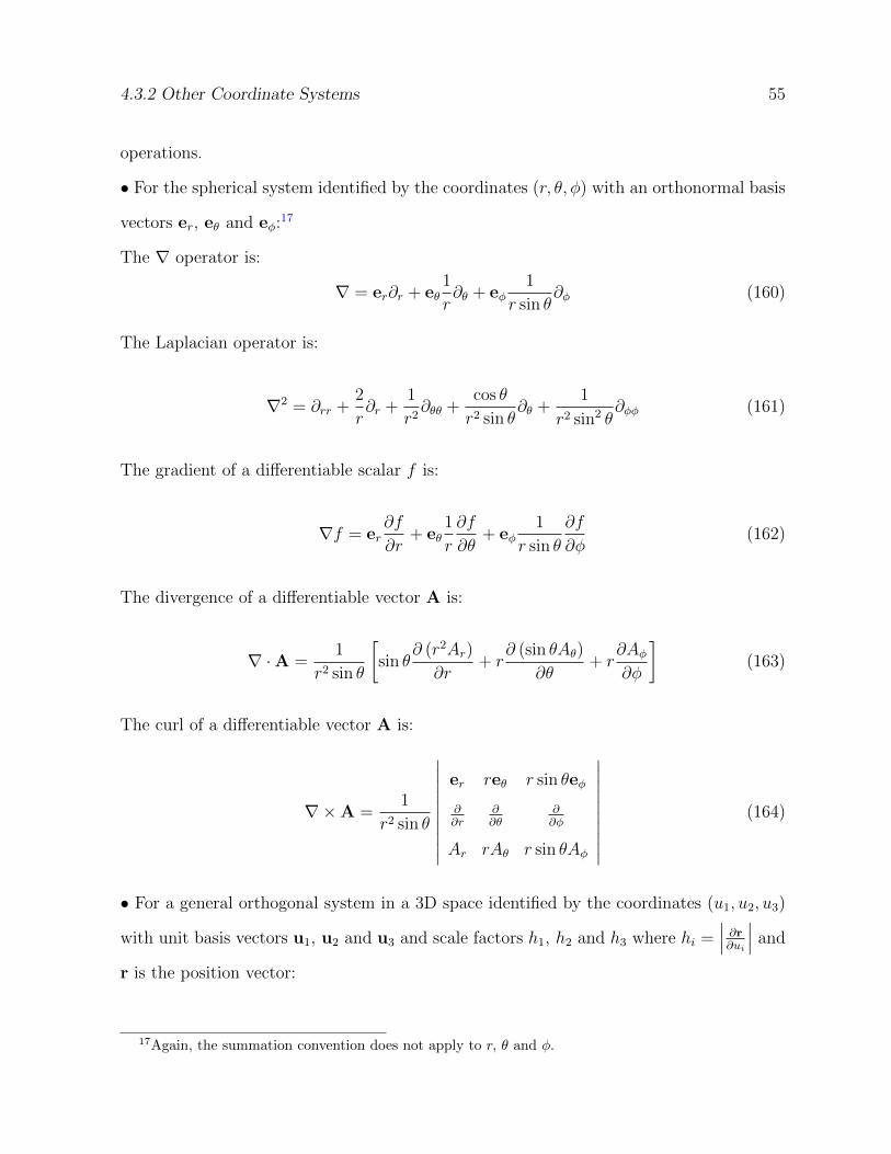
4.3.2 Other Coordinate Systems 55
operations.
• For the spherical system identified by the coordinates (r, θ, φ) with an orthonormal basis
vectors er, eθ and eφ:17
The ∇ operator is:
∇ = er∂r + eθ1
r∂θ + eφ
1
r sin θ∂φ (160)
The Laplacian operator is:
∇2 = ∂rr +2
r∂r +
1
r2∂θθ +
cos θ
r2 sin θ∂θ +
1
r2 sin2 θ∂φφ (161)
The gradient of a differentiable scalar f is:
∇f = er∂f
∂r+ eθ
1
r
∂f
∂θ+ eφ
1
r sin θ
∂f
∂φ(162)
The divergence of a differentiable vector A is:
∇ ·A =1
r2 sin θ
[sin θ
∂ (r2Ar)
∂r+ r
∂ (sin θAθ)
∂θ+ r
∂Aφ∂φ
](163)
The curl of a differentiable vector A is:
∇×A =1
r2 sin θ
∣∣∣∣∣∣∣∣∣∣er reθ r sin θeφ
∂∂r
∂∂θ
∂∂φ
Ar rAθ r sin θAφ
∣∣∣∣∣∣∣∣∣∣(164)
• For a general orthogonal system in a 3D space identified by the coordinates (u1, u2, u3)
with unit basis vectors u1, u2 and u3 and scale factors h1, h2 and h3 where hi =∣∣∣ ∂r∂ui ∣∣∣ and
r is the position vector:
17Again, the summation convention does not apply to r, θ and φ.
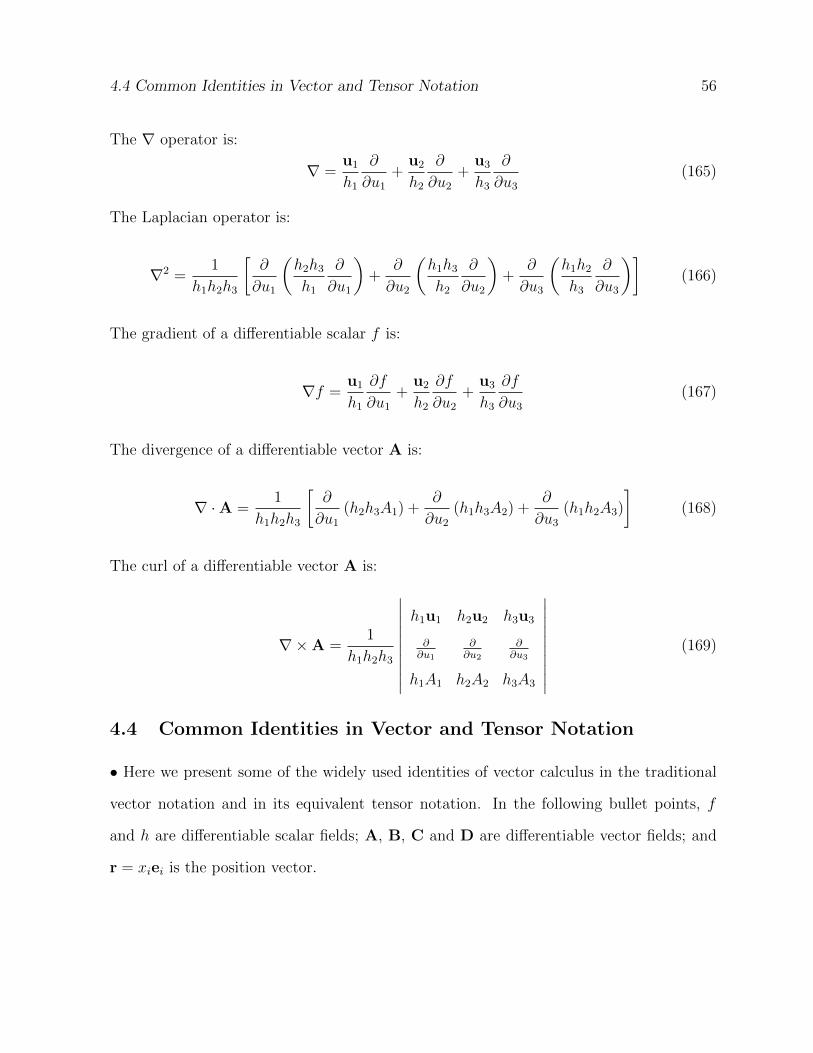
4.4 Common Identities in Vector and Tensor Notation 56
The ∇ operator is:
∇ =u1
h1
∂
∂u1
+u2
h2
∂
∂u2
+u3
h3
∂
∂u3
(165)
The Laplacian operator is:
∇2 =1
h1h2h3
[∂
∂u1
(h2h3
h1
∂
∂u1
)+
∂
∂u2
(h1h3
h2
∂
∂u2
)+
∂
∂u3
(h1h2
h3
∂
∂u3
)](166)
The gradient of a differentiable scalar f is:
∇f =u1
h1
∂f
∂u1
+u2
h2
∂f
∂u2
+u3
h3
∂f
∂u3
(167)
The divergence of a differentiable vector A is:
∇ ·A =1
h1h2h3
[∂
∂u1
(h2h3A1) +∂
∂u2
(h1h3A2) +∂
∂u3
(h1h2A3)
](168)
The curl of a differentiable vector A is:
∇×A =1
h1h2h3
∣∣∣∣∣∣∣∣∣∣h1u1 h2u2 h3u3
∂∂u1
∂∂u2
∂∂u3
h1A1 h2A2 h3A3
∣∣∣∣∣∣∣∣∣∣(169)
4.4 Common Identities in Vector and Tensor Notation
• Here we present some of the widely used identities of vector calculus in the traditional
vector notation and in its equivalent tensor notation. In the following bullet points, f
and h are differentiable scalar fields; A, B, C and D are differentiable vector fields; and
r = xiei is the position vector.
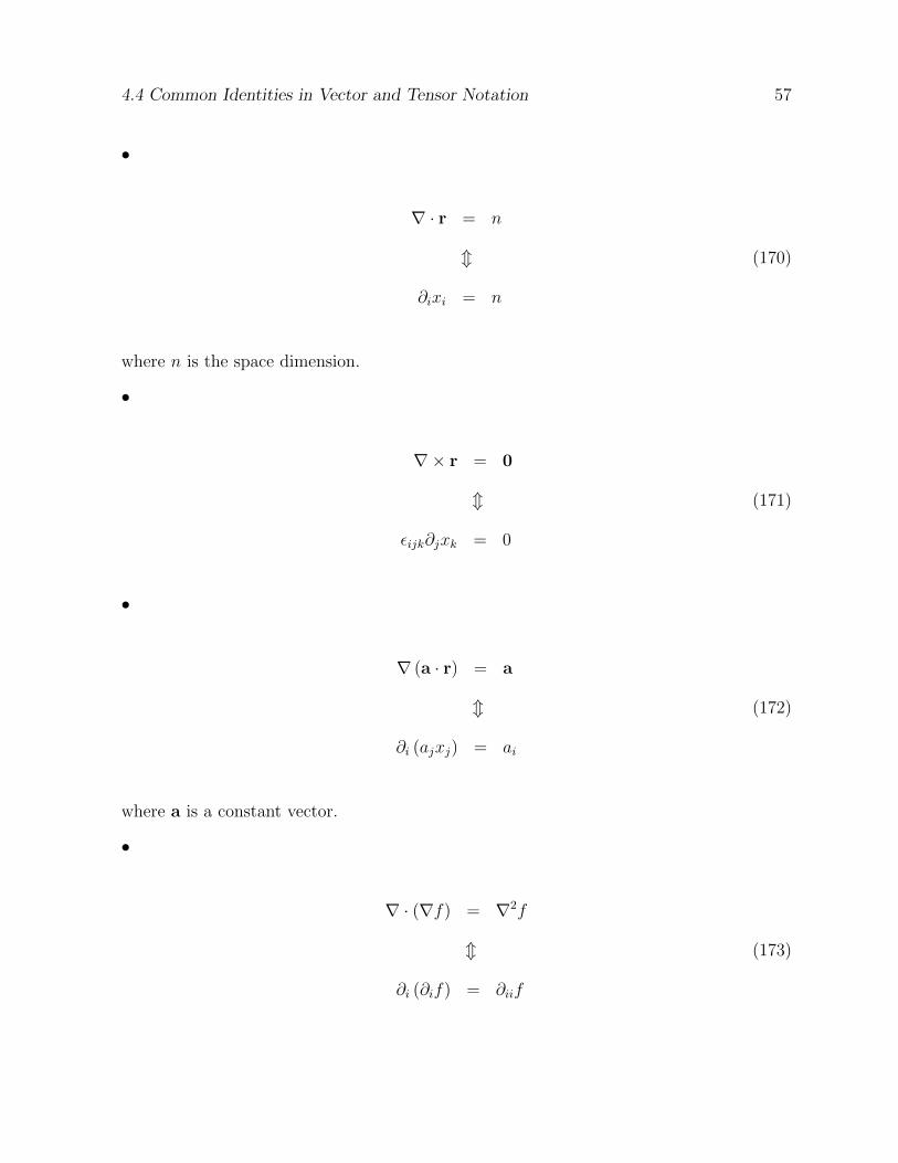
4.4 Common Identities in Vector and Tensor Notation 57
•
∇ · r = n
m (170)
∂ixi = n
where n is the space dimension.
•
∇ × r = 0
m (171)
εijk∂jxk = 0
•
∇ (a · r) = a
m (172)
∂i (ajxj) = ai
where a is a constant vector.
•
∇ · (∇f) = ∇2f
m (173)
∂i (∂if) = ∂iif
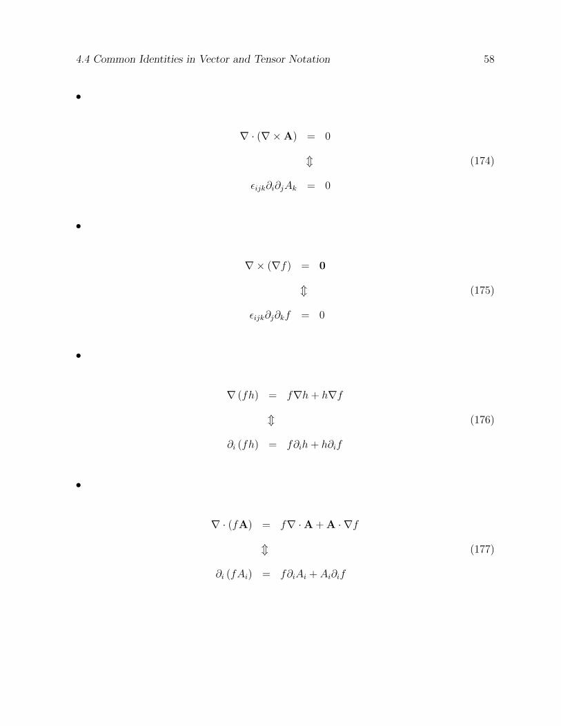
4.4 Common Identities in Vector and Tensor Notation 58
•
∇ · (∇×A) = 0
m (174)
εijk∂i∂jAk = 0
•
∇ × (∇f) = 0
m (175)
εijk∂j∂kf = 0
•
∇ (fh) = f∇h+ h∇f
m (176)
∂i (fh) = f∂ih+ h∂if
•
∇ · (fA) = f∇ ·A + A · ∇f
m (177)
∂i (fAi) = f∂iAi + Ai∂if
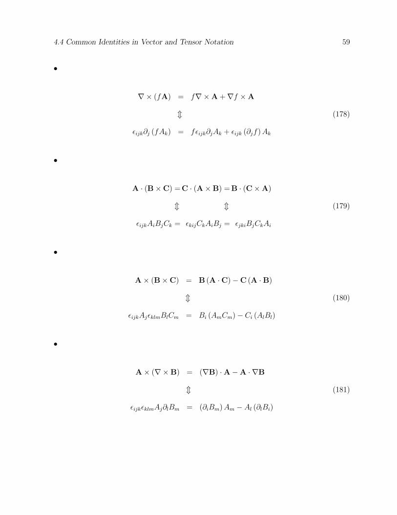
4.4 Common Identities in Vector and Tensor Notation 59
•
∇ × (fA) = f∇×A +∇f ×A
m (178)
εijk∂j (fAk) = fεijk∂jAk + εijk (∂jf)Ak
•
A · (B×C) = C · (A×B) = B · (C×A)
m m (179)
εijkAiBjCk = εkijCkAiBj = εjkiBjCkAi
•
A× (B×C) = B (A ·C)−C (A ·B)
m (180)
εijkAjεklmBlCm = Bi (AmCm)− Ci (AlBl)
•
A× (∇×B) = (∇B) ·A−A · ∇B
m (181)
εijkεklmAj∂lBm = (∂iBm)Am − Al (∂lBi)
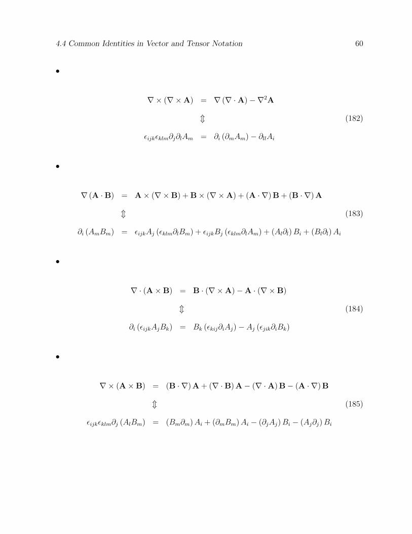
4.4 Common Identities in Vector and Tensor Notation 60
•
∇ × (∇×A) = ∇ (∇ ·A)−∇2A
m (182)
εijkεklm∂j∂lAm = ∂i (∂mAm)− ∂llAi
•
∇ (A ·B) = A× (∇×B) + B× (∇×A) + (A · ∇) B + (B · ∇) A
m (183)
∂i (AmBm) = εijkAj (εklm∂lBm) + εijkBj (εklm∂lAm) + (Al∂l)Bi + (Bl∂l)Ai
•
∇ · (A×B) = B · (∇×A)−A · (∇×B)
m (184)
∂i (εijkAjBk) = Bk (εkij∂iAj)− Aj (εjik∂iBk)
•
∇ × (A×B) = (B · ∇) A + (∇ ·B) A− (∇ ·A) B− (A · ∇) B
m (185)
εijkεklm∂j (AlBm) = (Bm∂m)Ai + (∂mBm)Ai − (∂jAj)Bi − (Aj∂j)Bi
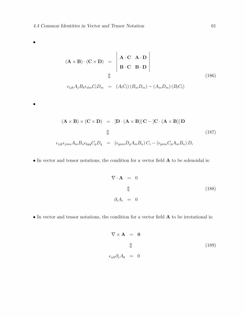
4.4 Common Identities in Vector and Tensor Notation 61
•
(A×B) · (C×D) =
∣∣∣∣∣∣∣A ·C A ·D
B ·C B ·D
∣∣∣∣∣∣∣m (186)
εijkAjBkεilmClDm = (AlCl) (BmDm)− (AmDm) (BlCl)
•
(A×B)× (C×D) = [D · (A×B)] C− [C · (A×B)] D
m (187)
εijkεjmnAmBnεkpqCpDq = (εqmnDqAmBn)Ci − (εpmnCpAmBn)Di
• In vector and tensor notations, the condition for a vector field A to be solenoidal is:
∇ ·A = 0
m (188)
∂iAi = 0
• In vector and tensor notations, the condition for a vector field A to be irrotational is:
∇×A = 0
m (189)
εijk∂jAk = 0
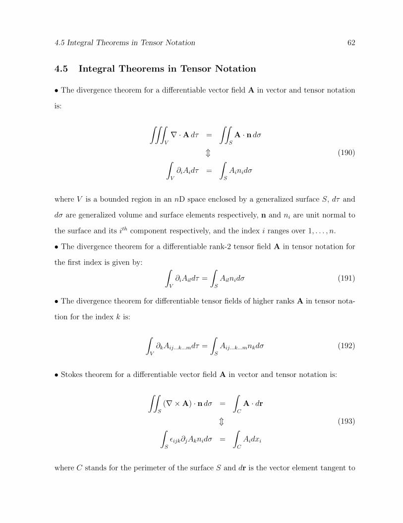
4.5 Integral Theorems in Tensor Notation 62
4.5 Integral Theorems in Tensor Notation
• The divergence theorem for a differentiable vector field A in vector and tensor notation
is:
∫∫∫V
∇ ·A dτ =
∫∫S
A · n dσ
m (190)∫V
∂iAidτ =
∫S
Ainidσ
where V is a bounded region in an nD space enclosed by a generalized surface S, dτ and
dσ are generalized volume and surface elements respectively, n and ni are unit normal to
the surface and its ith component respectively, and the index i ranges over 1, . . . , n.
• The divergence theorem for a differentiable rank-2 tensor field A in tensor notation for
the first index is given by: ∫V
∂iAildτ =
∫S
Ailnidσ (191)
• The divergence theorem for differentiable tensor fields of higher ranks A in tensor nota-
tion for the index k is:
∫V
∂kAij...k...mdτ =
∫S
Aij...k...mnkdσ (192)
• Stokes theorem for a differentiable vector field A in vector and tensor notation is:
∫∫S
(∇×A) · n dσ =
∫C
A · dr
m (193)∫S
εijk∂jAknidσ =
∫C
Aidxi
where C stands for the perimeter of the surface S and dr is the vector element tangent to
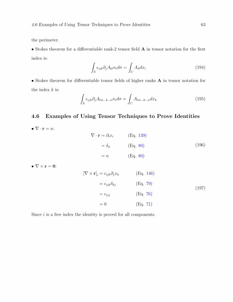
4.6 Examples of Using Tensor Techniques to Prove Identities 63
the perimeter.
• Stokes theorem for a differentiable rank-2 tensor field A in tensor notation for the first
index is: ∫S
εijk∂jAklnidσ =
∫C
Aildxi (194)
• Stokes theorem for differentiable tensor fields of higher ranks A in tensor notation for
the index k is: ∫S
εijk∂jAlm...k...nnidσ =
∫C
Alm...k...ndxk (195)
4.6 Examples of Using Tensor Techniques to Prove Identities
• ∇ · r = n:
∇ · r = ∂ixi (Eq. 139)
= δii (Eq. 80)
= n (Eq. 80)
(196)
• ∇ × r = 0:
[∇× r]i = εijk∂jxk (Eq. 146)
= εijkδkj (Eq. 79)
= εijj (Eq. 76)
= 0 (Eq. 71)
(197)
Since i is a free index the identity is proved for all components.
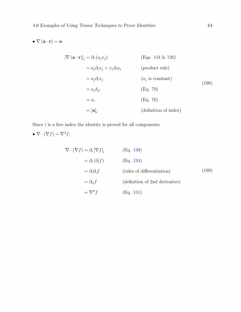
4.6 Examples of Using Tensor Techniques to Prove Identities 64
• ∇ (a · r) = a:
[∇ (a · r)]i = ∂i (ajxj) (Eqs. 134 & 120)
= aj∂ixj + xj∂iaj (product rule)
= aj∂ixj (aj is constant)
= ajδji (Eq. 79)
= ai (Eq. 76)
= [a]i (definition of index)
(198)
Since i is a free index the identity is proved for all components.
• ∇ · (∇f) = ∇2f :
∇ · (∇f) = ∂i [∇f ]i (Eq. 139)
= ∂i (∂if) (Eq. 134)
= ∂i∂if (rules of differentiation)
= ∂iif (definition of 2nd derivative)
= ∇2f (Eq. 151)
(199)
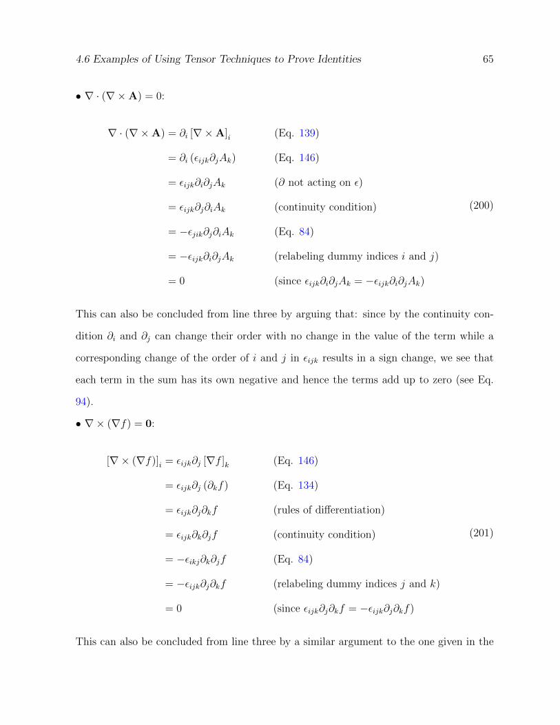
4.6 Examples of Using Tensor Techniques to Prove Identities 65
• ∇ · (∇×A) = 0:
∇ · (∇×A) = ∂i [∇×A]i (Eq. 139)
= ∂i (εijk∂jAk) (Eq. 146)
= εijk∂i∂jAk (∂ not acting on ε)
= εijk∂j∂iAk (continuity condition)
= −εjik∂j∂iAk (Eq. 84)
= −εijk∂i∂jAk (relabeling dummy indices i and j)
= 0 (since εijk∂i∂jAk = −εijk∂i∂jAk)
(200)
This can also be concluded from line three by arguing that: since by the continuity con-
dition ∂i and ∂j can change their order with no change in the value of the term while a
corresponding change of the order of i and j in εijk results in a sign change, we see that
each term in the sum has its own negative and hence the terms add up to zero (see Eq.
94).
• ∇ × (∇f) = 0:
[∇× (∇f)]i = εijk∂j [∇f ]k (Eq. 146)
= εijk∂j (∂kf) (Eq. 134)
= εijk∂j∂kf (rules of differentiation)
= εijk∂k∂jf (continuity condition)
= −εikj∂k∂jf (Eq. 84)
= −εijk∂j∂kf (relabeling dummy indices j and k)
= 0 (since εijk∂j∂kf = −εijk∂j∂kf)
(201)
This can also be concluded from line three by a similar argument to the one given in the
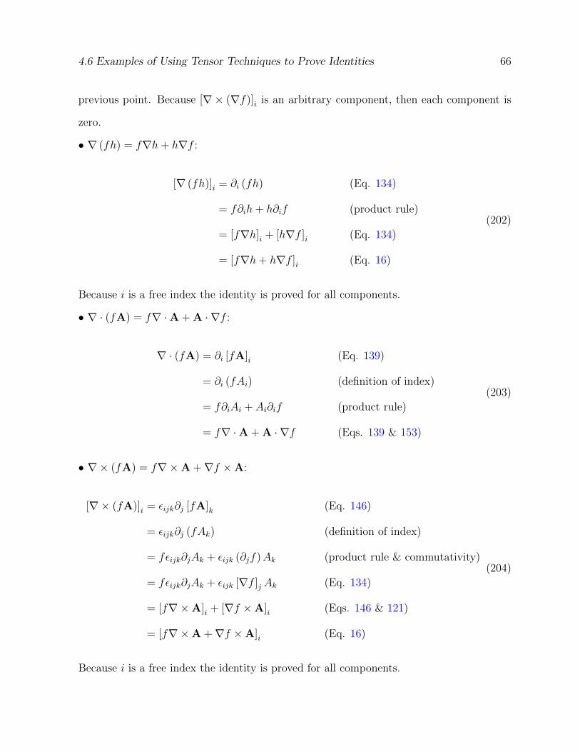
4.6 Examples of Using Tensor Techniques to Prove Identities 66
previous point. Because [∇× (∇f)]i is an arbitrary component, then each component is
zero.
• ∇ (fh) = f∇h+ h∇f :
[∇ (fh)]i = ∂i (fh) (Eq. 134)
= f∂ih+ h∂if (product rule)
= [f∇h]i + [h∇f ]i (Eq. 134)
= [f∇h+ h∇f ]i (Eq. 16)
(202)
Because i is a free index the identity is proved for all components.
• ∇ · (fA) = f∇ ·A + A · ∇f :
∇ · (fA) = ∂i [fA]i (Eq. 139)
= ∂i (fAi) (definition of index)
= f∂iAi + Ai∂if (product rule)
= f∇ ·A + A · ∇f (Eqs. 139 & 153)
(203)
• ∇ × (fA) = f∇×A +∇f ×A:
[∇× (fA)]i = εijk∂j [fA]k (Eq. 146)
= εijk∂j (fAk) (definition of index)
= fεijk∂jAk + εijk (∂jf)Ak (product rule & commutativity)
= fεijk∂jAk + εijk [∇f ]j Ak (Eq. 134)
= [f∇×A]i + [∇f ×A]i (Eqs. 146 & 121)
= [f∇×A +∇f ×A]i (Eq. 16)
(204)
Because i is a free index the identity is proved for all components.
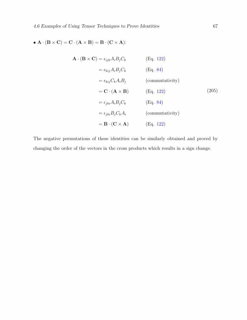
4.6 Examples of Using Tensor Techniques to Prove Identities 67
• A · (B×C) = C · (A×B) = B · (C×A):
A · (B×C) = εijkAiBjCk (Eq. 122)
= εkijAiBjCk (Eq. 84)
= εkijCkAiBj (commutativity)
= C · (A×B) (Eq. 122)
= εjkiAiBjCk (Eq. 84)
= εjkiBjCkAi (commutativity)
= B · (C×A) (Eq. 122)
(205)
The negative permutations of these identities can be similarly obtained and proved by
changing the order of the vectors in the cross products which results in a sign change.

4.6 Examples of Using Tensor Techniques to Prove Identities 68
• A× (B×C) = B (A ·C)−C (A ·B):
[A× (B×C)]i = εijkAj [B×C]k (Eq. 121)
= εijkAjεklmBlCm (Eq. 121)
= εijkεklmAjBlCm (commutativity)
= εijkεlmkAjBlCm (Eq. 84)
= (δilδjm − δimδjl)AjBlCm (Eq. 102)
= δilδjmAjBlCm − δimδjlAjBlCm (distributivity)
= (δilBl) (δjmAjCm)− (δimCm) (δjlAjBl) (commutativity and grouping)
= Bi (AmCm)− Ci (AlBl) (Eq. 76)
= Bi (A ·C)− Ci (A ·B) (Eq. 120)
= [B (A ·C)]i − [C (A ·B)]i (definition of index)
= [B (A ·C)−C (A ·B)]i (Eq. 16)
(206)
Because i is a free index the identity is proved for all components. Other variants of this
identity [e.g. (A×B) × C] can be obtained and proved similarly by changing the order
of the factors in the external cross product with adding a minus sign.
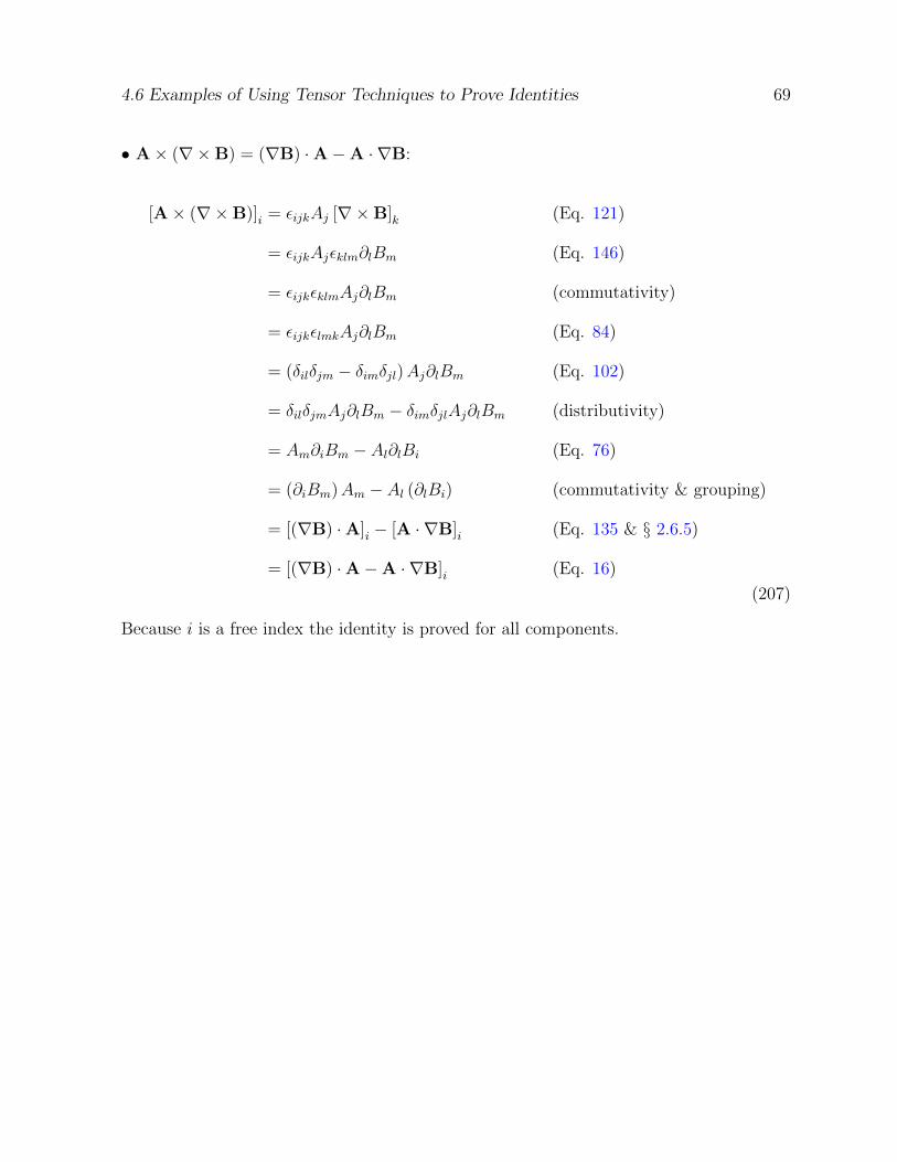
4.6 Examples of Using Tensor Techniques to Prove Identities 69
• A× (∇×B) = (∇B) ·A−A · ∇B:
[A× (∇×B)]i = εijkAj [∇×B]k (Eq. 121)
= εijkAjεklm∂lBm (Eq. 146)
= εijkεklmAj∂lBm (commutativity)
= εijkεlmkAj∂lBm (Eq. 84)
= (δilδjm − δimδjl)Aj∂lBm (Eq. 102)
= δilδjmAj∂lBm − δimδjlAj∂lBm (distributivity)
= Am∂iBm − Al∂lBi (Eq. 76)
= (∂iBm)Am − Al (∂lBi) (commutativity & grouping)
= [(∇B) ·A]i − [A · ∇B]i (Eq. 135 & § 2.6.5)
= [(∇B) ·A−A · ∇B]i (Eq. 16)
(207)
Because i is a free index the identity is proved for all components.
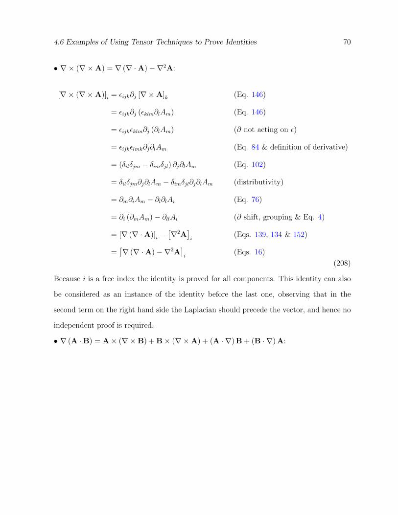
4.6 Examples of Using Tensor Techniques to Prove Identities 70
• ∇ × (∇×A) = ∇ (∇ ·A)−∇2A:
[∇× (∇×A)]i = εijk∂j [∇×A]k (Eq. 146)
= εijk∂j (εklm∂lAm) (Eq. 146)
= εijkεklm∂j (∂lAm) (∂ not acting on ε)
= εijkεlmk∂j∂lAm (Eq. 84 & definition of derivative)
= (δilδjm − δimδjl) ∂j∂lAm (Eq. 102)
= δilδjm∂j∂lAm − δimδjl∂j∂lAm (distributivity)
= ∂m∂iAm − ∂l∂lAi (Eq. 76)
= ∂i (∂mAm)− ∂llAi (∂ shift, grouping & Eq. 4)
= [∇ (∇ ·A)]i −[∇2A
]i
(Eqs. 139, 134 & 152)
=[∇ (∇ ·A)−∇2A
]i
(Eqs. 16)
(208)
Because i is a free index the identity is proved for all components. This identity can also
be considered as an instance of the identity before the last one, observing that in the
second term on the right hand side the Laplacian should precede the vector, and hence no
independent proof is required.
• ∇ (A ·B) = A× (∇×B) + B× (∇×A) + (A · ∇) B + (B · ∇) A:
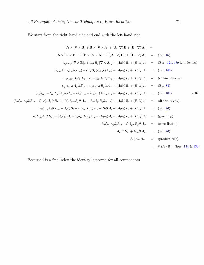
4.6 Examples of Using Tensor Techniques to Prove Identities 71
We start from the right hand side and end with the left hand side
[A× (∇×B) + B× (∇×A) + (A · ∇)B + (B · ∇)A]i =
[A× (∇×B)]i + [B× (∇×A)]i + [(A · ∇)B]i + [(B · ∇)A]i = (Eq. 16)
εijkAj [∇×B]k + εijkBj [∇×A]k + (Al∂l)Bi + (Bl∂l)Ai = (Eqs. 121, 139 & indexing)
εijkAj (εklm∂lBm) + εijkBj (εklm∂lAm) + (Al∂l)Bi + (Bl∂l)Ai = (Eq. 146)
εijkεklmAj∂lBm + εijkεklmBj∂lAm + (Al∂l)Bi + (Bl∂l)Ai = (commutativity)
εijkεlmkAj∂lBm + εijkεlmkBj∂lAm + (Al∂l)Bi + (Bl∂l)Ai = (Eq. 84)
(δilδjm − δimδjl)Aj∂lBm + (δilδjm − δimδjl)Bj∂lAm + (Al∂l)Bi + (Bl∂l)Ai = (Eq. 102) (209)
(δilδjmAj∂lBm − δimδjlAj∂lBm) + (δilδjmBj∂lAm − δimδjlBj∂lAm) + (Al∂l)Bi + (Bl∂l)Ai = (distributivity)
δilδjmAj∂lBm −Al∂lBi + δilδjmBj∂lAm −Bl∂lAi + (Al∂l)Bi + (Bl∂l)Ai = (Eq. 76)
δilδjmAj∂lBm − (Al∂l)Bi + δilδjmBj∂lAm − (Bl∂l)Ai + (Al∂l)Bi + (Bl∂l)Ai = (grouping)
δilδjmAj∂lBm + δilδjmBj∂lAm = (cancellation)
Am∂iBm +Bm∂iAm = (Eq. 76)
∂i (AmBm) = (product rule)
= [∇ (A ·B)]i (Eqs. 134 & 139)
Because i is a free index the identity is proved for all components.
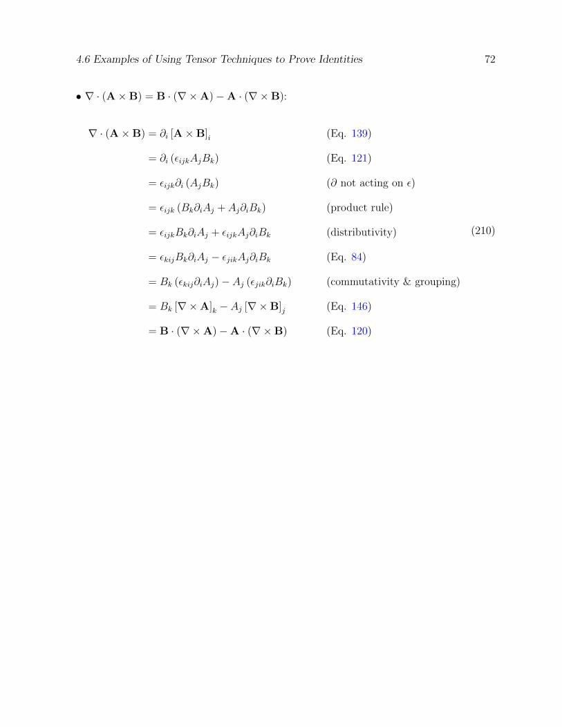
4.6 Examples of Using Tensor Techniques to Prove Identities 72
• ∇ · (A×B) = B · (∇×A)−A · (∇×B):
∇ · (A×B) = ∂i [A×B]i (Eq. 139)
= ∂i (εijkAjBk) (Eq. 121)
= εijk∂i (AjBk) (∂ not acting on ε)
= εijk (Bk∂iAj + Aj∂iBk) (product rule)
= εijkBk∂iAj + εijkAj∂iBk (distributivity)
= εkijBk∂iAj − εjikAj∂iBk (Eq. 84)
= Bk (εkij∂iAj)− Aj (εjik∂iBk) (commutativity & grouping)
= Bk [∇×A]k − Aj [∇×B]j (Eq. 146)
= B · (∇×A)−A · (∇×B) (Eq. 120)
(210)

4.6 Examples of Using Tensor Techniques to Prove Identities 73
• ∇ × (A×B) = (B · ∇) A + (∇ ·B) A− (∇ ·A) B− (A · ∇) B:
[∇× (A×B)]i = εijk∂j [A×B]k (Eq. 146)
= εijk∂j (εklmAlBm) (Eq. 121)
= εijkεklm∂j (AlBm) (∂ not acting on ε)
= εijkεklm (Bm∂jAl + Al∂jBm) (product rule)
= εijkεlmk (Bm∂jAl + Al∂jBm) (Eq. 84)
= (δilδjm − δimδjl) (Bm∂jAl + Al∂jBm) (Eq. 102)
= δilδjmBm∂jAl + δilδjmAl∂jBm − δimδjlBm∂jAl − δimδjlAl∂jBm (distributivity)
= Bm∂mAi + Ai∂mBm −Bi∂jAj − Aj∂jBi (Eq. 76)
= (Bm∂m)Ai + (∂mBm)Ai − (∂jAj)Bi − (Aj∂j)Bi (grouping)
= [(B · ∇) A]i + [(∇ ·B) A]i − [(∇ ·A) B]i − [(A · ∇) B]i (Eqs. 153 & 139)
= [(B · ∇) A + (∇ ·B) A− (∇ ·A) B− (A · ∇) B]i (Eq. 16)
(211)
Because i is a free index the identity is proved for all components.
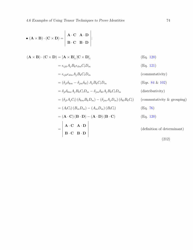
4.6 Examples of Using Tensor Techniques to Prove Identities 74
• (A×B) · (C×D) =
∣∣∣∣∣∣∣A ·C A ·D
B ·C B ·D
∣∣∣∣∣∣∣:
(A×B) · (C×D) = [A×B]i [C×D]i (Eq. 120)
= εijkAjBkεilmClDm (Eq. 121)
= εijkεilmAjBkClDm (commutativity)
= (δjlδkm − δjmδkl)AjBkClDm (Eqs. 84 & 102)
= δjlδkmAjBkClDm − δjmδklAjBkClDm (distributivity)
= (δjlAjCl) (δkmBkDm)− (δjmAjDm) (δklBkCl) (commutativity & grouping)
= (AlCl) (BmDm)− (AmDm) (BlCl) (Eq. 76)
= (A ·C) (B ·D)− (A ·D) (B ·C) (Eq. 120)
=
∣∣∣∣∣∣∣A ·C A ·D
B ·C B ·D
∣∣∣∣∣∣∣ (definition of determinant)
(212)
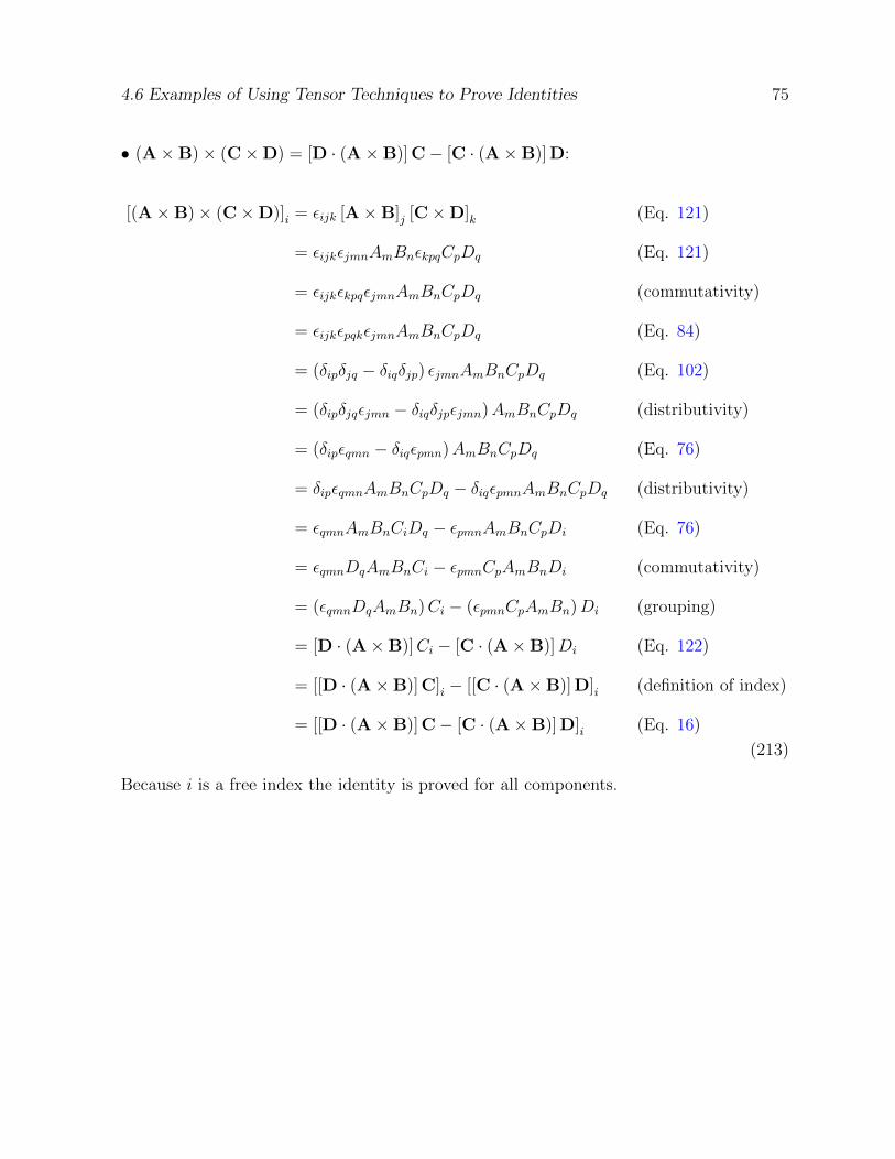
4.6 Examples of Using Tensor Techniques to Prove Identities 75
• (A×B)× (C×D) = [D · (A×B)] C− [C · (A×B)] D:
[(A×B)× (C×D)]i = εijk [A×B]j [C×D]k (Eq. 121)
= εijkεjmnAmBnεkpqCpDq (Eq. 121)
= εijkεkpqεjmnAmBnCpDq (commutativity)
= εijkεpqkεjmnAmBnCpDq (Eq. 84)
= (δipδjq − δiqδjp) εjmnAmBnCpDq (Eq. 102)
= (δipδjqεjmn − δiqδjpεjmn)AmBnCpDq (distributivity)
= (δipεqmn − δiqεpmn)AmBnCpDq (Eq. 76)
= δipεqmnAmBnCpDq − δiqεpmnAmBnCpDq (distributivity)
= εqmnAmBnCiDq − εpmnAmBnCpDi (Eq. 76)
= εqmnDqAmBnCi − εpmnCpAmBnDi (commutativity)
= (εqmnDqAmBn)Ci − (εpmnCpAmBn)Di (grouping)
= [D · (A×B)]Ci − [C · (A×B)]Di (Eq. 122)
= [[D · (A×B)] C]i − [[C · (A×B)] D]i (definition of index)
= [[D · (A×B)] C− [C · (A×B)] D]i (Eq. 16)
(213)
Because i is a free index the identity is proved for all components.
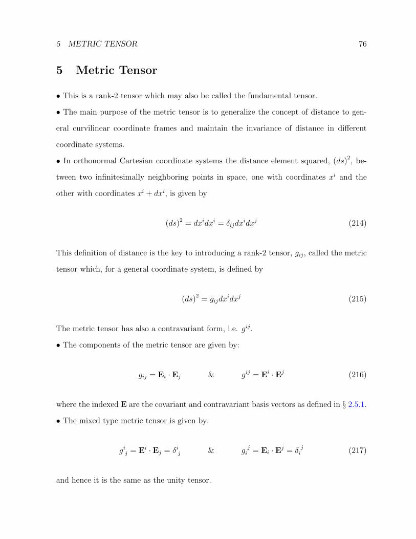
5 METRIC TENSOR 76
5 Metric Tensor
• This is a rank-2 tensor which may also be called the fundamental tensor.
• The main purpose of the metric tensor is to generalize the concept of distance to gen-
eral curvilinear coordinate frames and maintain the invariance of distance in different
coordinate systems.
• In orthonormal Cartesian coordinate systems the distance element squared, (ds)2, be-
tween two infinitesimally neighboring points in space, one with coordinates xi and the
other with coordinates xi + dxi, is given by
(ds)2 = dxidxi = δijdxidxj (214)
This definition of distance is the key to introducing a rank-2 tensor, gij, called the metric
tensor which, for a general coordinate system, is defined by
(ds)2 = gijdxidxj (215)
The metric tensor has also a contravariant form, i.e. gij.
• The components of the metric tensor are given by:
gij = Ei · Ej & gij = Ei · Ej (216)
where the indexed E are the covariant and contravariant basis vectors as defined in § 2.5.1.
• The mixed type metric tensor is given by:
gij = Ei · Ej = δij & g ji = Ei · Ej = δ ji (217)
and hence it is the same as the unity tensor.
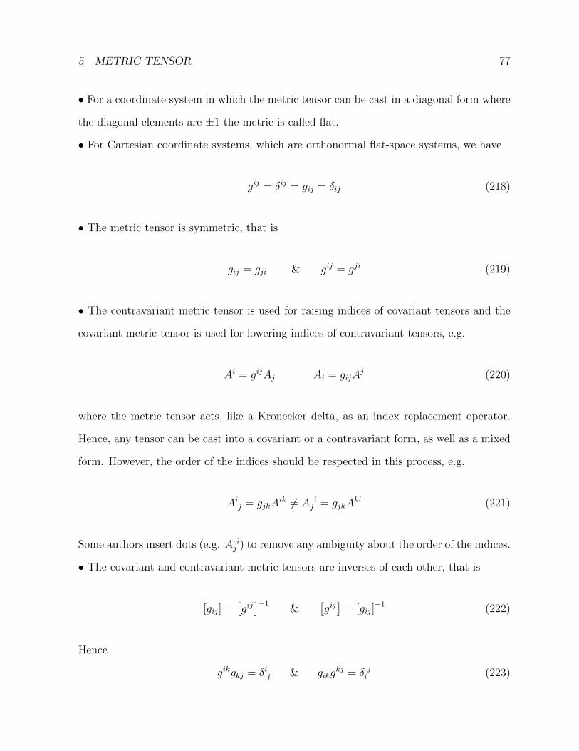
5 METRIC TENSOR 77
• For a coordinate system in which the metric tensor can be cast in a diagonal form where
the diagonal elements are ±1 the metric is called flat.
• For Cartesian coordinate systems, which are orthonormal flat-space systems, we have
gij = δij = gij = δij (218)
• The metric tensor is symmetric, that is
gij = gji & gij = gji (219)
• The contravariant metric tensor is used for raising indices of covariant tensors and the
covariant metric tensor is used for lowering indices of contravariant tensors, e.g.
Ai = gijAj Ai = gijAj (220)
where the metric tensor acts, like a Kronecker delta, as an index replacement operator.
Hence, any tensor can be cast into a covariant or a contravariant form, as well as a mixed
form. However, the order of the indices should be respected in this process, e.g.
Aij = gjkAik 6= A i
j = gjkAki (221)
Some authors insert dots (e.g. A· ij ) to remove any ambiguity about the order of the indices.
• The covariant and contravariant metric tensors are inverses of each other, that is
[gij] =[gij]−1
&[gij]
= [gij]−1 (222)
Hence
gikgkj = δij & gikgkj = δ ji (223)
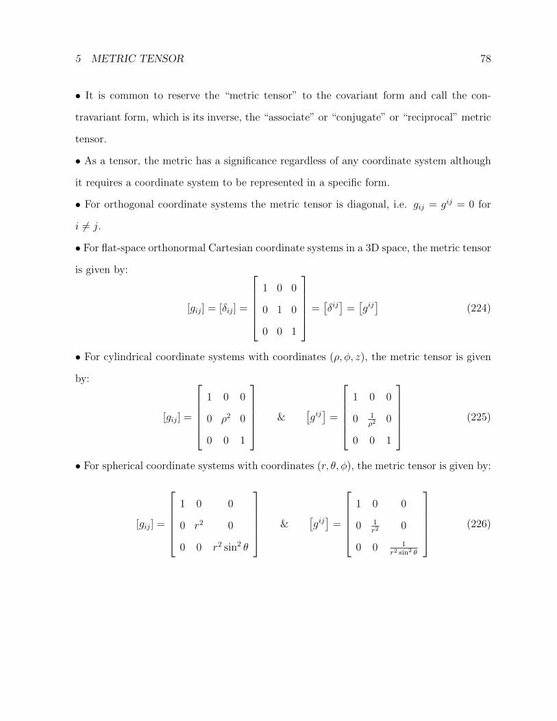
5 METRIC TENSOR 78
• It is common to reserve the “metric tensor” to the covariant form and call the con-
travariant form, which is its inverse, the “associate” or “conjugate” or “reciprocal” metric
tensor.
• As a tensor, the metric has a significance regardless of any coordinate system although
it requires a coordinate system to be represented in a specific form.
• For orthogonal coordinate systems the metric tensor is diagonal, i.e. gij = gij = 0 for
i 6= j.
• For flat-space orthonormal Cartesian coordinate systems in a 3D space, the metric tensor
is given by:
[gij] = [δij] =
1 0 0
0 1 0
0 0 1
=[δij]
=[gij]
(224)
• For cylindrical coordinate systems with coordinates (ρ, φ, z), the metric tensor is given
by:
[gij] =
1 0 0
0 ρ2 0
0 0 1
&[gij]
=
1 0 0
0 1ρ2
0
0 0 1
(225)
• For spherical coordinate systems with coordinates (r, θ, φ), the metric tensor is given by:
[gij] =
1 0 0
0 r2 0
0 0 r2 sin2 θ
&[gij]
=
1 0 0
0 1r2
0
0 0 1r2 sin2 θ
(226)
6 COVARIANT DIFFERENTIATION 79
6 Covariant Differentiation
• The ordinary derivative of a tensor is not a tensor in general. The objective of covariant
differentiation is to ensure the invariance of derivative (i.e. being a tensor) in general
coordinate systems, and this results in applying more sophisticated rules using Christof-
fel symbols where different differentiation rules for covariant and contravariant indices
apply. The resulting covariant derivative is a tensor which is one rank higher than the
differentiated tensor.
• Christoffel symbol of the second kind is defined by:
{kij
}=gkl
2
(∂gil∂xj
+∂gjl∂xi− ∂gij∂xl
)(227)
where the indexed g is the metric tensor in its contravariant and covariant forms with
implied summation over l. It is noteworthy that Christoffel symbols are not tensors.
• The Christoffel symbols of the second kind are symmetric in their two lower indices:
{kij
}={kji
}(228)
• For Cartesian coordinate systems, the Christoffel symbols are zero for all the values of
indices.
• For cylindrical coordinate systems (ρ, φ, z), the Christoffel symbols are zero for all the
values of indices except:
{122
}= −ρ (229){
212
}=
{221
}=
1
ρ
where (1, 2, 3) stand for (ρ, φ, z).
6 COVARIANT DIFFERENTIATION 80
• For spherical coordinate systems (r, θ, φ), the Christoffel symbols are zero for all the
values of indices except:
{122
}= −r (230){
133
}= −r sin2 θ{
212
}=
{221
}=
1
r{233
}= − sin θ cos θ{
313
}=
{331
}=
1
r{323
}=
{332
}= cot θ
where (1, 2, 3) stand for (r, θ, φ).
• For a differentiable scalar f the covariant derivative is the same as the normal partial
derivative, that is:
f;i = f,i = ∂if (231)
This is justified by the fact that the covariant derivative is different from the normal partial
derivative because the basis vectors in general coordinate systems are dependent on their
spatial position, and since a scalar is independent of the basis vectors the covariant and
partial derivatives are identical.
• For a differentiable vector A the covariant derivative is:
Aj;i = ∂iAj −{kji
}Ak (covariant)
Aj;i = ∂iAj +{jki
}Ak (contravariant)
(232)
6 COVARIANT DIFFERENTIATION 81
• For a differentiable rank-2 tensor A the covariant derivative is:
Ajk;i = ∂iAjk −{lji
}Alk −
{lki
}Ajl (covariant)
Ajk;i = ∂iAjk +
{jli
}Alk +
{kli
}Ajl (contravariant)
Akj;i = ∂iAkj +
{kli
}Alj −
{lji
}Akl (mixed)
(233)
• For a differentiable rank-n tensor A the covariant derivative is:
Aij...klm...p;q = ∂qAij...klm...p +
{iaq
}Aaj...klm...p +
{jaq
}Aia...klm...p + · · ·+
{kaq
}Aij...alm...p (234)
−{alq
}Aij...kam...p −
{amq
}Aij...kla...p − · · · −
{apq
}Aij...klm...a
• From the last three points a pattern for covariant differentiation emerges, that is it starts
with a partial derivative term then for each tensor index an extra Christoffel symbol term
is added, positive for superscripts and negative for subscripts, where the differentiation
index is the second of the lower indices in the Christoffel symbol.
• Since the Christoffel symbols are identically zero in Cartesian coordinate systems, the
covariant derivative is the same as the normal partial derivative for all tensor ranks.
• The covariant derivative of the metric tensor is zero in all coordinate systems.
• Several rules of normal differentiation similarly apply to covariant differentiation. For
example, covariant differentiation is a linear operation with respect to algebraic sums of
tensor terms:
∂;i (aA± bB) = a∂;iA± b∂;iB (235)
where a and b are scalar constants and A and B are differentiable tensor fields. The
product rule of normal differentiation also applies to covariant differentiation of tensor
multiplication:
∂;i (AB) = (∂;iA) B + A∂;iB (236)
6 COVARIANT DIFFERENTIATION 82
This rule is also valid for the inner product of tensors because the inner product is an
outer product operation followed by a contraction of indices, and covariant differentiation
and contraction of indices commute.
• The covariant derivative operator can bypass the raising/lowering index operator:
Ai = gijAj =⇒ ∂;mAi = gij∂;mA
j (237)
and hence the metric behaves like a constant with respect to the covariant operator.
• A principal difference between normal partial differentiation and covariant differentiation
is that for successive differential operations the partial derivative operators do commute
with each other (assuming certain continuity conditions) but the covariant operators do
not commute, that is
∂i∂j = ∂j∂i but ∂;i∂;j 6= ∂;j∂;i (238)
• Higher order covariant derivatives are similarly defined as derivatives of derivatives;
however the order of differentiation should be respected (refer to the previous point).
REFERENCES 83
References
[1] G.B. Arfken; H.J. Weber; F.E. Harris. Mathematical Methods for Physicists A Com-
prehensive Guide. Elsevier Academic Press, seventh edition, 2013.
[2] R.B. Bird; R.C. Armstrong; O. Hassager. Dynamics of Polymeric Liquids, volume 1.
John Wiley & Sons, second edition, 1987.
[3] R.B. Bird; W.E. Stewart; E.N. Lightfoot. Transport Phenomena. John Wiley & Sons,
second edition, 2002.
[4] M.L. Boas. Mathematical Methods in the Physical Sciences. John Wiley & Sons Inc.,
third edition, 2006.
[5] C.F. Chan Man Fong; D. De Kee; P.N. Kaloni. Advanced Mathematics for Engineering
and Science. World Scientific Publishing Co. Pte. Ltd., first edition, 2003.
[6] T.L. Chow. Mathematical Methods for Physicists: A concise introduction. Cambridge
University Press, first edition, 2003.
[7] J.H. Heinbockel. Introduction to Tensor Calculus and Continuum Mechanics. 1996.
[8] D.C. Kay. Schaum’s Outline of Theory and Problems of Tensor Calculus. McGraw-
Hill, first edition, 1988.
[9] K.F. Riley; M.P. Hobson; S.J. Bence. Mathematical Methods for Physics and Engi-
neering. Cambridge University Press, third edition, 2006.
[10] D. Zwillinger, editor. CRC Standard Mathematical Tables and Formulae. CRC Press,
32nd edition, 2012.
Note: As well as the references cited above, I benefited during the writing of these notes
from many sources such as tutorials, presentations, and articles which I found on the
REFERENCES 84
Internet authored or composed by other people. As it is difficult or impossible to retrace
and state all these sources, I make a general acknowledgment to all those who made their
documents available to the public.