introduction to theoretical elementary particle physics
TRANSCRIPT
Introduction to Theoretical Elementary Particle
Physics:
Relativistic Quantum Field Theory
Part I
Stefan Weinzierl
July 6, 2020
1
Contents
1 Overview 4
1.1 Literature . . . . . . . . . . . . . . . . . . . . . . . . . . . . . . . . . . . . . . 4
1.2 Units . . . . . . . . . . . . . . . . . . . . . . . . . . . . . . . . . . . . . . . . . 4
1.3 The fundamental forces . . . . . . . . . . . . . . . . . . . . . . . . . . . . . . . 5
1.4 The elementary particles . . . . . . . . . . . . . . . . . . . . . . . . . . . . . . 6
1.4.1 Spin 1/2 particles . . . . . . . . . . . . . . . . . . . . . . . . . . . . . . 6
1.4.2 Spin 1 particles . . . . . . . . . . . . . . . . . . . . . . . . . . . . . . . 7
1.4.3 Spin 0 particles . . . . . . . . . . . . . . . . . . . . . . . . . . . . . . . 8
1.5 Experiments . . . . . . . . . . . . . . . . . . . . . . . . . . . . . . . . . . . . . 8
1.6 Observed, but not elementary particles . . . . . . . . . . . . . . . . . . . . . . . 9
2 Review of quantum mechanics 10
2.1 The harmonic oscillator in classical mechanics . . . . . . . . . . . . . . . . . . . 10
2.2 The harmonic oscillator in quantum mechanics . . . . . . . . . . . . . . . . . . 10
2.2.1 Operator formalism . . . . . . . . . . . . . . . . . . . . . . . . . . . . . 11
2.2.2 Path integrals . . . . . . . . . . . . . . . . . . . . . . . . . . . . . . . . 14
2.2.3 Summary . . . . . . . . . . . . . . . . . . . . . . . . . . . . . . . . . . 16
3 Review of special relativity 17
3.1 Four-vectors and the metric . . . . . . . . . . . . . . . . . . . . . . . . . . . . . 17
3.2 The Lorentz group . . . . . . . . . . . . . . . . . . . . . . . . . . . . . . . . . 18
3.3 The Poincaré group . . . . . . . . . . . . . . . . . . . . . . . . . . . . . . . . . 21
4 Review of classical field theory 22
4.1 The action principle . . . . . . . . . . . . . . . . . . . . . . . . . . . . . . . . . 22
4.2 Examples of classical fields . . . . . . . . . . . . . . . . . . . . . . . . . . . . . 24
4.2.1 The Klein-Gordon field . . . . . . . . . . . . . . . . . . . . . . . . . . . 24
4.2.2 The Dirac field . . . . . . . . . . . . . . . . . . . . . . . . . . . . . . . 25
4.2.3 The Maxwell field . . . . . . . . . . . . . . . . . . . . . . . . . . . . . 26
5 Quantum field theory: The canonical formalism 28
5.1 The Klein-Gordon field as harmonic oscillators . . . . . . . . . . . . . . . . . . 28
5.2 The Schrödinger picture . . . . . . . . . . . . . . . . . . . . . . . . . . . . . . 30
5.3 The Fock space . . . . . . . . . . . . . . . . . . . . . . . . . . . . . . . . . . . 35
5.4 The Heisenberg picture . . . . . . . . . . . . . . . . . . . . . . . . . . . . . . . 36
5.4.1 Causality . . . . . . . . . . . . . . . . . . . . . . . . . . . . . . . . . . 38
5.4.2 The Klein-Gordon propagator . . . . . . . . . . . . . . . . . . . . . . . 39
5.5 Wick’s theorem . . . . . . . . . . . . . . . . . . . . . . . . . . . . . . . . . . . 42
5.6 Interacting fields . . . . . . . . . . . . . . . . . . . . . . . . . . . . . . . . . . 44
5.7 Feynman diagrams . . . . . . . . . . . . . . . . . . . . . . . . . . . . . . . . . 50
5.8 Summary: Feynman rules for φ4-theory in momentum space . . . . . . . . . . . 55
2
6 Cross sections and decay rates 56
6.1 The S-matrix . . . . . . . . . . . . . . . . . . . . . . . . . . . . . . . . . . . . 58
6.2 Properties of the S-matrix . . . . . . . . . . . . . . . . . . . . . . . . . . . . . . 63
6.3 Relation between invariant matrix elements and Feynman diagrams . . . . . . . . 64
6.4 Final formula . . . . . . . . . . . . . . . . . . . . . . . . . . . . . . . . . . . . 65
7 Fermions 67
7.1 The Dirac equation . . . . . . . . . . . . . . . . . . . . . . . . . . . . . . . . . 67
7.2 Massless spinors . . . . . . . . . . . . . . . . . . . . . . . . . . . . . . . . . . 68
7.3 Spinorproducts . . . . . . . . . . . . . . . . . . . . . . . . . . . . . . . . . . . 71
7.4 Massive spinors . . . . . . . . . . . . . . . . . . . . . . . . . . . . . . . . . . . 72
7.5 Quantisation of fermions . . . . . . . . . . . . . . . . . . . . . . . . . . . . . . 73
7.6 Feynman rules for fermions . . . . . . . . . . . . . . . . . . . . . . . . . . . . . 75
7.7 Rules for traces over Dirac matrices . . . . . . . . . . . . . . . . . . . . . . . . 76
8 Quantum field theory via path integrals 78
8.1 Trouble with the canonical quantisation of gauge bosons . . . . . . . . . . . . . 79
8.2 Path integrals . . . . . . . . . . . . . . . . . . . . . . . . . . . . . . . . . . . . 80
8.3 Transition amplitudes as path integrals . . . . . . . . . . . . . . . . . . . . . . . 82
8.4 Correlation functions . . . . . . . . . . . . . . . . . . . . . . . . . . . . . . . . 85
8.5 Fermions in the path integral formalism . . . . . . . . . . . . . . . . . . . . . . 87
8.5.1 Grassmann numbers . . . . . . . . . . . . . . . . . . . . . . . . . . . . 87
8.5.2 Path integrals with fermions . . . . . . . . . . . . . . . . . . . . . . . . 89
8.6 The reduction formula of Lehmann, Symanzik and Zimmermann . . . . . . . . . 89
9 Gauge theories 94
9.1 Lie groups und Lie algebras . . . . . . . . . . . . . . . . . . . . . . . . . . . . 94
9.2 Special unitary Lie groups . . . . . . . . . . . . . . . . . . . . . . . . . . . . . 96
9.3 Yang-Mills theory . . . . . . . . . . . . . . . . . . . . . . . . . . . . . . . . . . 97
9.4 Quantisation of gauge theories . . . . . . . . . . . . . . . . . . . . . . . . . . . 98
9.5 The Lagrange density for the fermion sector . . . . . . . . . . . . . . . . . . . . 103
9.6 Feynman rules for QED and QCD . . . . . . . . . . . . . . . . . . . . . . . . . 104
9.6.1 Propagators . . . . . . . . . . . . . . . . . . . . . . . . . . . . . . . . . 104
9.6.2 Vertices . . . . . . . . . . . . . . . . . . . . . . . . . . . . . . . . . . . 106
9.6.3 List of Feynman rules . . . . . . . . . . . . . . . . . . . . . . . . . . . 107
9.7 Colour decomposition . . . . . . . . . . . . . . . . . . . . . . . . . . . . . . . . 110
10 Example calculations for scattering amplitudes 115
10.1 Examples from QED: Bhabha, Møller and annihilation . . . . . . . . . . . . . . 115
10.2 Calculation of helicity amplitudes . . . . . . . . . . . . . . . . . . . . . . . . . 118
3
1 Overview
1.1 Literature
There is no shortage of text books on quantum field theory. I will list a few of them here:
- M. Peskin und D. Schroeder, An Introduction to Quantum Field Theory, Perseus Books, 1995.
- M. Schwartz, Quantum Field Theory and the Standard Model, Cambridge University Press,
2014.
- M. Srednicki, Quantum Field Theory, Cambridge University Press, 2007.
- D. Bailin und A. Love, Introduction to Gauge Field Theory, A. Hilger, 1986.
- T. Muta, Foundations of Quantum Chromodynamics, World Scientific, 1987.
- M. Böhm, A. Denner and H. Joos, Gauge Theories of the Strong and Electroweak Interactions,
Teubner, 2001.
- C. Itzykson and J.-B. Zuber, Quantum Field Theory, McGraw-Hill, 1980.
- J.D. Bjorken and S.D. Drell, Relativistic Quantum Mechanics, McGraw-Hill, 1964.
- J.D. Bjorken and S.D. Drell, Relativistic Quantum Fields, McGraw-Hill, 1965.
1.2 Units
It is common practice in quantum field theory and elementary particle physics to use natural
units. Thus, by convention we set
~= c = 1.
For example, the equation
E2− c2~p2 = m2c4
simplifies to
E2−~p2 = m2.
We will use this convention in these lectures. To facilitate the transition to this convention, we
will still write in the very beginning of this course the quantities ~ and c explicitly, but soon set
them equal to one as we proceed.
Energy is measured in eV:
1 eV = 1.6021764 ·10−19J.
4
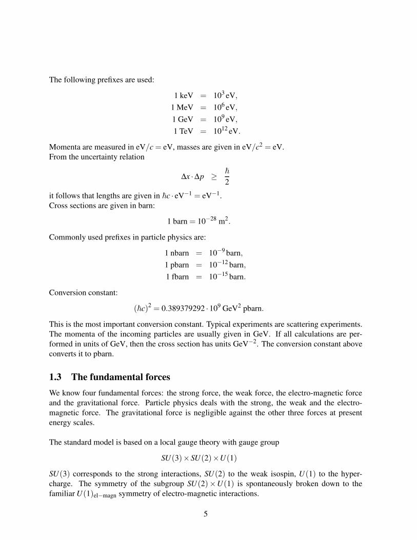
The following prefixes are used:
1 keV = 103 eV,
1 MeV = 106 eV,
1 GeV = 109 eV,
1 TeV = 1012 eV.
Momenta are measured in eV/c = eV, masses are given in eV/c2 = eV.
From the uncertainty relation
∆x ·∆p ≥ ~
2
it follows that lengths are given in ~c · eV−1 = eV−1.
Cross sections are given in barn:
1 barn = 10−28 m2.
Commonly used prefixes in particle physics are:
1 nbarn = 10−9 barn,
1 pbarn = 10−12 barn,
1 fbarn = 10−15 barn.
Conversion constant:
(~c)2 = 0.389379292 ·109 GeV2 pbarn.
This is the most important conversion constant. Typical experiments are scattering experiments.
The momenta of the incoming particles are usually given in GeV. If all calculations are per-
formed in units of GeV, then the cross section has units GeV−2. The conversion constant above
converts it to pbarn.
1.3 The fundamental forces
We know four fundamental forces: the strong force, the weak force, the electro-magnetic force
and the gravitational force. Particle physics deals with the strong, the weak and the electro-
magnetic force. The gravitational force is negligible against the other three forces at present
energy scales.
The standard model is based on a local gauge theory with gauge group
SU(3)×SU(2)×U(1)
SU(3) corresponds to the strong interactions, SU(2) to the weak isospin, U(1) to the hyper-
charge. The symmetry of the subgroup SU(2)×U(1) is spontaneously broken down to the
familiar U(1)el−magn symmetry of electro-magnetic interactions.
5
1.4 The elementary particles
The spin of the particles:
- Fermions have half-integer spin. In the standard model all fermions have spin 1/2. In exten-
sions of the standard model higher spins may occur, e.g. the gravitino with spin 3/2.
- Bosons have integer spin. In the standard model all bosons have either spin 1 (gauge bosons)
or spin 0 (Higgs boson). In extensions of the standard model there might be particles of
higher spin, e.g. a graviton of spin 2.
1.4.1 Spin 1/2 particles
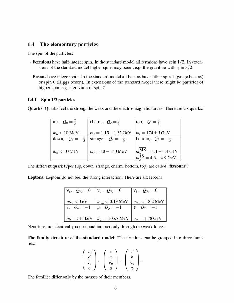
Quarks: Quarks feel the strong, the weak and the electro-magnetic forces. There are six quarks:
up, Qu =23
charm, Qc =23
top, Qt =23
mu < 10 MeV mc = 1.15−1.35 GeV mt = 174±5 GeV
down, Qd =−13
strange, Qs =−13
bottom, Qb =−13
md < 10 MeV ms = 80−130 MeV mMSb = 4.1−4.4 GeV
m1Sb = 4.6−4.9 GeV
The different quark types (up, down, strange, charm, bottom, top) are called “flavours”.
Leptons: Leptons do not feel the strong interaction. There are six leptons:
νe, Qνe= 0 νµ, Qνµ
= 0 ντ, Qντ = 0
mνe< 3 eV mνµ
< 0.19 MeV mντ < 18.2 MeV
e, Qe =−1 µ, Qµ =−1 τ, Qτ =−1
me = 511 keV mµ = 105.7 MeV mτ = 1.78 GeV
Neutrinos are electrically neutral and interact only through the weak force.
The family structure of the standard model: The fermions can be grouped into three fami-
lies:
u
d
νe
e
,
c
s
νµ
µ
,
t
b
ντ
τ
.
The families differ only by the masses of their members.
6
1.4.2 Spin 1 particles
Within the standard model the mediators of the interactions are spin 1 particles.
The strong interaction: SU(3): The gauge group SU(3) describes the strong interaction. The
number of generators for a group SU(N) is N2− 1, therefore there are 8 generators for SU(3),and hence 8 gauge bosons for the strong interactions. The gauge bosons of the strong interaction
are called gluons. The fields are denoted by
Aaµ,
where a runs from 1 to 8.
The weak isospin: SU(2): The weak interaction is described by the gauge group SU(2). There
are three generators
W 1µ ,W
2µ ,W
3µ ,
each with two polarisation states. After electro-weak symmetry breaking we use the fields
W+µ ,W−µ ,Zµ,
with three polarisation states. We have the following relations:
W±µ =1√2
(W 1
µ ∓ iW 2µ
),
Zµ = −sinθW Bµ + cosθwW 3µ .
The third spin degree of freedom comes from the Higgs mechanism.
The hypercharge: U(1): The last piece of gauge-symmetries within the standard model is given
by an abelian U(1) gauge symmetry, the hypercharge. The field is denoted by
Bµ
After electro-weak symmetry breaking the photon field Aµ is given as a linear combination of Bµ
and W 3µ :
Aµ = cosθW Bµ + sinθwW 3µ .
Note that(
Aµ
Zµ
)
=
(cosθW sinθW
−sinθW cosθW
)(Bµ
W 3µ
)
and that Aµ remains a massless field with two polarisation states.
7
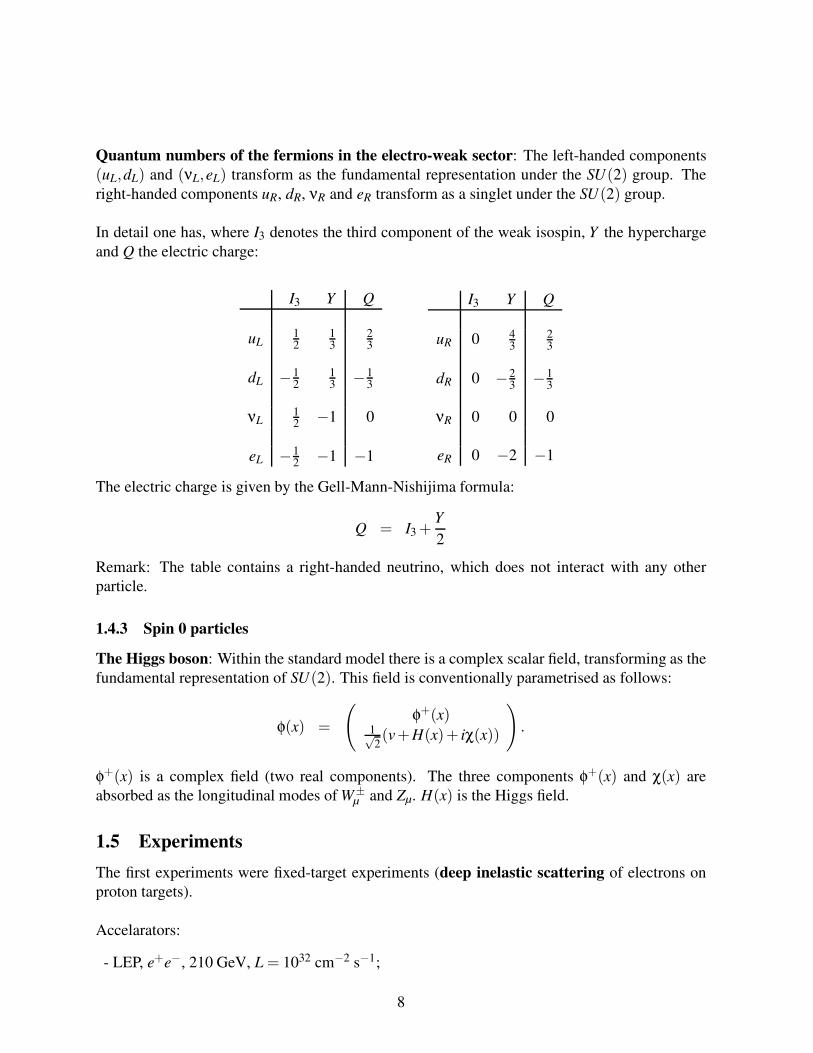
Quantum numbers of the fermions in the electro-weak sector: The left-handed components
(uL,dL) and (νL,eL) transform as the fundamental representation under the SU(2) group. The
right-handed components uR, dR, νR and eR transform as a singlet under the SU(2) group.
In detail one has, where I3 denotes the third component of the weak isospin, Y the hypercharge
and Q the electric charge:
I3 Y Q
uL12
13
23
dL −12
13−1
3
νL12−1 0
eL −12−1 −1
I3 Y Q
uR 0 43
23
dR 0 −23−1
3
νR 0 0 0
eR 0 −2 −1
The electric charge is given by the Gell-Mann-Nishijima formula:
Q = I3 +Y
2
Remark: The table contains a right-handed neutrino, which does not interact with any other
particle.
1.4.3 Spin 0 particles
The Higgs boson: Within the standard model there is a complex scalar field, transforming as the
fundamental representation of SU(2). This field is conventionally parametrised as follows:
φ(x) =
(
φ+(x)1√2(v+H(x)+ iχ(x))
)
.
φ+(x) is a complex field (two real components). The three components φ+(x) and χ(x) are
absorbed as the longitudinal modes of W±µ and Zµ. H(x) is the Higgs field.
1.5 Experiments
The first experiments were fixed-target experiments (deep inelastic scattering of electrons on
proton targets).
Accelarators:
- LEP, e+e−, 210 GeV, L = 1032 cm−2 s−1;
8

- TEVATRON, pp, 1.96 TeV, L = 5 ·1030 cm−2 s−1;
- HERA, e−p, e− : 30 GeV, p : 960 GeV, L = 75 ·1030 cm−2 s−1;
- LHC, pp, 14 TeV, L = 1034 cm−2 s−1;
- Linear Collider (planned), e+e−, 500 GeV, L = 5 ·1034 cm−2 s−1;
Quarks and gluons are not directly observed in these experiments. Instead one observes hadronic
jets. A jet is a bunch of particles moving in the same direction. Particles in a jet are not neces-
sarily elementary.
1.6 Observed, but not elementary particles
Due to confinement, quarks and gluons cannot be observed as free particles. In experiments
we observe particles which are colour-singlets like mesons and baryons. Within the quark
model, mesons are qq-states and baryons qqq-states. Mesons and baryons are called collec-
tively hadrons.
Examples are:
Mesons: Pions, kaons, η’s, D-mesons, J/ψ, ...
Baryons: protons, neutrons, Σ, Ξ, ...
9
2 Review of quantum mechanics
2.1 The harmonic oscillator in classical mechanics
Let us start with classical mechanics and recall the Lagrange and Hamilton description of the
non-relativistic harmonic oscillator in classical mechanics. The Lagrange function for the har-
monic oscillator reads
L =1
2mx2− 1
2mω2x2.
From the Euler-Lagrange equation
d
dt
δL
δx− δL
δx= 0
follows the equation of motion
x+ω2x2 = 0,
which has the solution
x(t) = Aeiωt +Be−iωt .
Remark: The conjugate momentum is given by
p =δL
δx= mx,
and the Hamilton function reads
H = px−L =1
2mx2 +
1
2mω2x2 =
p2
2m+
1
2mω2x2.
2.2 The harmonic oscillator in quantum mechanics
In quantum mechanics the harmonic oscillator is described by a wave function ψ(x, t). This wave
function can be expanded into an orthonormal basis. We denote by |x; t0〉H a wave function in the
Heisenberg picture, which is at the time t = t0 an eigenvector of the Heisenberg position operator
xH(t) with eigenvalue x:
xH(t0) |x; t0〉H = x |x; t0〉H .
In general, the position operator does not commute with the Hamilton operator, therefore for
t 6= t0 the state will in general not be an eigenstate of xH(t). Furthermore we remark that a state
in the Heisenberg picture is time-independent. The label t0 refers to the time, where the state
|x; t0〉 is an eigenvector of the time-dependent position operator xH(t). The relation between the
states in the Heisenberg picture and in the Schrödinger picture is
|x; t0〉H = eiHt |x, t; t0〉S .
10
At time t = t0 the Schrödinger state |x, t0; t0〉 is an eigenstate of the Schrödinger position operator
xS:
xS |x, t0; t0〉S = x |x, t0; t0〉S.
We are interested in the transition amplitude
H〈x f ; t f |xi; ti〉H ,
which gives us the probability that the system which was in the eigenstate |xi; ti〉H at time ti will
be found in the state |x f ; t f 〉H at time t f . We discuss the transition amplitude for pedagocical pur-
poses: On the one hand, the transition amplitude can be worked out in non-relativistic quantum
mechanics. On the other hand, the transition amplitude is already close to objects (scattering
amplitudes), which we will study in quantum field theory. We will discuss two methods for
the calculation of the transition amplitude: one method based on operators, the other on path
integrals. Both methods have a generalisation to quantum field theory.
2.2.1 Operator formalism
Let us first compute the transition amplitude with the operator formalism. This is the standard
method treated in most textbooks of quantum mechanics. Here, we present only the main formu-
lae, but do not give any derivations.
The time evolution of the wave function in the Schrödinger picture is given by the Schrödinger
equation
i~∂
∂tψ(x, t) = Hψ(x, t),
where the Hamilton operator is given by
H =p2
2m+
1
2mω2x2.
We make the ansatz
ψ(x, t) = U(t, ti)|x, ti; ti〉S
The evolution operator satisfies the equation
i~∂
∂tU(t, ti) = HU(t, ti).
If the Hamilton operator is time-independent (as it is for the harmonic oscillator), the solution
for U(t, ti) is given by
U(t, ti) = exp
(
− i
~(t− ti) · H
)
.
11
Remark: If the Hamilton operator H depends on the time t, a formal solution for U(t, ti) is given
by
U(t, ti) = T exp
− i
~
t∫
ti
dt ′H(t ′)
.
Here, T denotes the time-ordering operator, which orders operators from right to left in non-
decreasing time. Expanding the exponential one obtains
U(t, ti) = 1− i
~
t∫
ti
dt1H(t1)+
(i
~
)2 t∫
ti
dt1H(t1)
t1∫
ti
dt2H(t2)
−(
i
~
)3 t∫
ti
dt1H(t1)
t1∫
ti
dt2H(t2)
t2∫
ti
dt3H(t3)+ ....
Note that the factor 1/n! disappears.
To determine U(t, ti)|x, ti; ti〉S we expand |x, ti; ti〉S into eigenstates of the Hamilton operator.
These eigenstates will be labelled |n〉 and we have
H|n〉 = En|n〉.
Therefore
U(t, ti)|x, ti; ti〉S = exp
(
− i
~(t− ti) · H
)
|x, ti; ti〉S = ∑n
e−i~(t−ti)En|n〉〈n|x, ti; ti〉S.
To find these eigenstates we define two operators
a =ωmx+ ip√
2ωm~, a† =
ωmx− ip√2ωm~
.
If we introduce the characteristic length
x0 =
√
~
ωm,
we can equally write them as
a =1√2
(x
x0+ x0
d
dx
)
, a† =1√2
(x
x0− x0
d
dx
)
.
a is called lowering operator or annihilation operator, a† is called raising operator or creation
operator. From
[x, p] =
[
x,h
i
d
dx
]
= i~
12
it follows that[
a, a†]
= 1.
The Hamilton operator can be rewritten as
H =1
2~ω(
a†a+ aa†)
= ~ω
(
a†a+1
2
)
.
We call
N = a†a
the number operator and the problem of finding the energy eigenstates is reduced to the problem
of finding the eigenstates of the number operator. We have
n〈n|n〉= 〈n|N|n〉= 〈n|a†an〉= 〈an|an〉 ≥ 0.
Therefore n ≥ 0 and the lowest energy state corresponds to n = 0. Since the norm of a|0〉 van-
ishes, we have
a|0〉 = 0,(
d
dx+
x
x20
)
|0〉 = 0.
A solution is given by
|0〉 =(√
πx0
)− 12 exp
(
−1
2
(x
x0
)2)
.
One easily shows that
• a†|n〉 is an eigenstate with eigenvalue n+1.
• a|n〉 is an eigenstate with eigenvalue n−1.
Therefore one finds
|n〉 =1√n!
(
a†)n
|0〉=(2nn!√
πx0
)− 12 exp
(
−1
2
(x
x0
)2)
Hn
(x
x0
)
,
where Hn(t) are the Hermite polynomials.
The corresponding energies are given by
En = ~ω
(
n+1
2
)
.
Finally, we get
H〈x f ; t f |xi; ti〉H = ∑n
S〈x f , t f ; t f |n〉e−i~(t f−ti)En〈n|x, ti; ti〉S.
13
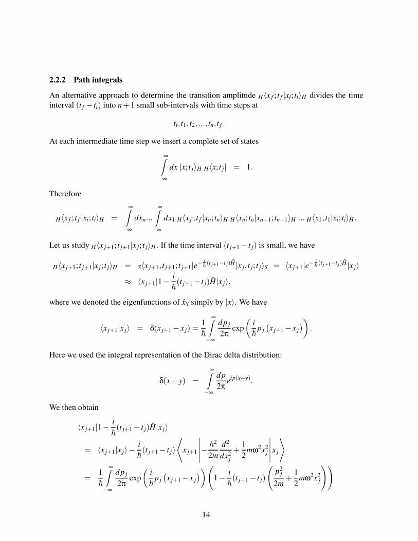
2.2.2 Path integrals
An alternative approach to determine the transition amplitude H〈x f ; t f |xi; ti〉H divides the time
interval (t f − ti) into n+1 small sub-intervals with time steps at
ti, t1, t2, ..., tn, t f .
At each intermediate time step we insert a complete set of states
∞∫
−∞
dx |x; t j〉H H〈x; t j| = 1.
Therefore
H〈x f ; t f |xi; ti〉H =
∞∫
−∞
dxn...
∞∫
−∞
dx1 H〈x f ; t f |xn; tn〉H H〈xn; tn|xn−1; tn−1〉H ... H〈x1; t1|xi; ti〉H .
Let us study H〈x j+1; t j+1|x j; t j〉H . If the time interval (t j+1− t j) is small, we have
H〈x j+1; t j+1|x j; t j〉H = S〈x j+1, t j+1; t j+1|e−i~(t j+1−t j)H |x j, t j; t j〉S = 〈x j+1|e−
i~(t j+1−t j)H |x j〉
≈ 〈x j+1|1−i
~(t j+1− t j)H|x j〉,
where we denoted the eigenfunctions of xS simply by |x〉. We have
〈x j+1|x j〉 = δ(x j+1− x j) =1
~
∞∫
−∞
dp j
2πexp
(i
~p j
(x j+1− x j
))
.
Here we used the integral representation of the Dirac delta distribution:
δ(x− y) =
∞∫
−∞
dp
2πeip(x−y).
We then obtain
〈x j+1|1−i
~(t j+1− t j)H|x j〉
= 〈x j+1|x j〉−i
~(t j+1− t j)
⟨
x j+1
∣∣∣∣∣− ~2
2m
d2
dx2j
+1
2mω2x2
j
∣∣∣∣∣x j
⟩
=1
~
∞∫
−∞
dp j
2πexp
(i
~p j
(x j+1− x j
))(
1− i
~(t j+1− t j)
(
p2j
2m+
1
2mω2x2
j
))
14
=1
~
∞∫
−∞
dp j
2πexp
(i
~p j
(x j+1− x j
))(
1− i
~(t j+1− t j)H(x j, p j)
)
≈ 1
~
∞∫
−∞
dp j
2πexp
(i
~p j
(x j+1− x j
)− i
~(t j+1− t j)H(x j, p j)
)
≈ 1
~
∞∫
−∞
dp j
2πexp
(i
~(t j+1− t j)
(p jx j−H(x j, p j)
))
.
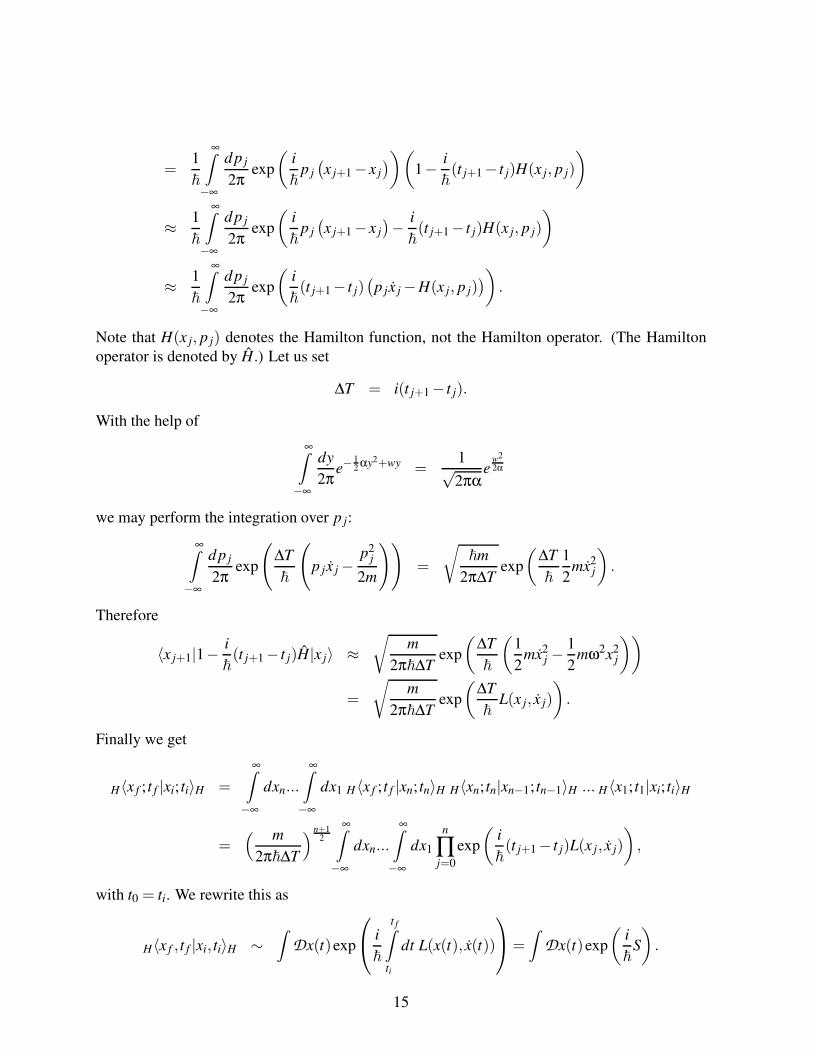
Note that H(x j, p j) denotes the Hamilton function, not the Hamilton operator. (The Hamilton
operator is denoted by H.) Let us set
∆T = i(t j+1− t j).
With the help of
∞∫
−∞
dy
2πe−
12 αy2+wy =
1√2πα
ew2
2α
we may perform the integration over p j:
∞∫
−∞
dp j
2πexp
(
∆T
~
(
p j x j−p2
j
2m
))
=
√
~m
2π∆Texp
(∆T
~
1
2mx2
j
)
.
Therefore
〈x j+1|1−i
~(t j+1− t j)H|x j〉 ≈
√m
2π~∆Texp
(∆T
~
(1
2mx2
j −1
2mω2x2
j
))
=
√m
2π~∆Texp
(∆T
~L(x j, x j)
)
.
Finally we get
H〈x f ; t f |xi; ti〉H =
∞∫
−∞
dxn...
∞∫
−∞
dx1 H〈x f ; t f |xn; tn〉H H〈xn; tn|xn−1; tn−1〉H ... H〈x1; t1|xi; ti〉H
=( m
2π~∆T
) n+12
∞∫
−∞
dxn...
∞∫
−∞
dx1
n
∏j=0
exp
(i
~(t j+1− t j)L(x j, x j)
)
,
with t0 = ti. We rewrite this as
H〈x f , t f |xi, ti〉H ∼∫
Dx(t)exp
i
~
t f∫
ti
dt L(x(t), x(t))
=∫
Dx(t)exp
(i
~S
)
.
15
Note the appearance of the Lagrange function L(x(t), x(t)) and the action
S =
t f∫
ti
dt L(x(t), x(t)).
2.2.3 Summary
The quantum mechanical harmonic oscillator shows already several concepts, which will reap-
pear later in quantum field theory. These are:
• Annihilation and creation operators.
• Transition amplitudes can be expressed as path integrals.
• The appearance of the Lagrange function and the action in the path integral.
16
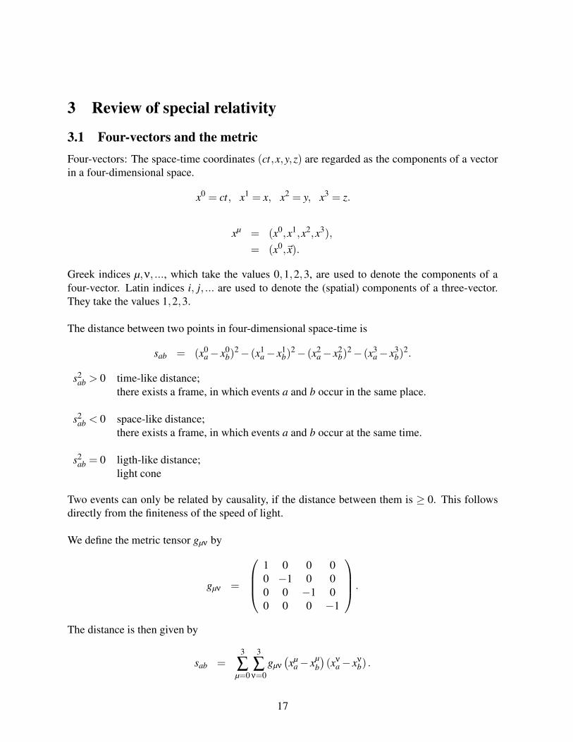
3 Review of special relativity
3.1 Four-vectors and the metric
Four-vectors: The space-time coordinates (ct,x,y,z) are regarded as the components of a vector
in a four-dimensional space.
x0 = ct, x1 = x, x2 = y, x3 = z.
xµ = (x0,x1,x2,x3),
= (x0,~x).
Greek indices µ,ν, ..., which take the values 0,1,2,3, are used to denote the components of a
four-vector. Latin indices i, j, ... are used to denote the (spatial) components of a three-vector.
They take the values 1,2,3.
The distance between two points in four-dimensional space-time is
sab = (x0a− x0
b)2− (x1
a− x1b)
2− (x2a− x2
b)2− (x3
a− x3b)
2.
s2ab > 0 time-like distance;
there exists a frame, in which events a and b occur in the same place.
s2ab < 0 space-like distance;
there exists a frame, in which events a and b occur at the same time.
s2ab = 0 ligth-like distance;
light cone
Two events can only be related by causality, if the distance between them is ≥ 0. This follows
directly from the finiteness of the speed of light.
We define the metric tensor gµν by
gµν =
1 0 0 0
0 −1 0 0
0 0 −1 0
0 0 0 −1
.
The distance is then given by
sab =3
∑µ=0
3
∑ν=0
gµν
(xµ
a− xµb
)(xν
a− xνb) .
17
Summation convention of Einstein: The symbol of the sum is dropped and it is understood, that
there is an implicit summation over any pair of indices, which occurs twice. Within a pait, one
index has to be an upper index, the other one a lower index. Therefore:
sab = gµν (xa− xb)µ (xa− xb)
ν .
We call a four-vector xµ with an upper index a contravariant four-vector, and we call a four-vector
xµ with a lower index a covariant four-vector. The relation between the two is given by
xµ = gµνxν.
Therefore we can write the distance equally as
sab = (xa− xb)µ (xa− xb)µ = (xa− xb)
µ (xa− xb)µ .
Remark: The geometry defined by the quadratic form gµν = diag(1,−1,−1,−1) is non-Euclidean.
The special case of a four-dimensional space with metric diag(1,−1,−1,−1) is often called
Minkowski space.
3.2 The Lorentz group
Axioms for a group: Let G be a non-empty set with a binary operation. G is called a group, if it
satisfies the axioms
• Associativity: a · (b · c) = (a ·b) · c.
• Existence of a neutral element: e ·a = a.
• Existence of an inverse: a−1 ·a = e.
Definition of the Lorentz group: Matrix group, which leaves the metric tensor gµν = diag(1,−1,−1,−1)invariant:
ΛT gΛ = g,
The same equation with indices:
ΛµσgµνΛν
τ = gστ.
This group is denoted O(1,3). It is easy to show that
(det Λ)2 = 1,
and therefore
det Λ = ±1.
18
If we have in addition det Λ = 1 the corresponding group is called the “proper” Lorentz group
and denoted SO(1,3).One further distinguishes the cases whether the time direction is conserved or reversed. If
Λ00 ≥ 1,
the time direction is conserved and the corresponding group is called the orthochronous Lorentz
group. If on the other hand
Λ00 ≤ −1,
then the time direction is reversed. Remark:∣∣Λ0
0
∣∣ ≥ 1
follows from ΛµσgµνΛν
τ = gστ for σ = τ = 0:
(Λ0
0
)2−3
∑j=1
(
Λj0
)2
= 1.
To summarise: The Lorentz group consists of four components, depending on which values the
quantities
det Λ and Λ00
take. The “proper orthochronous Lorentz group” is defined by
ΛµσgµνΛν
τ = gστ, det Λ = 1, Λ00 ≥ 1,
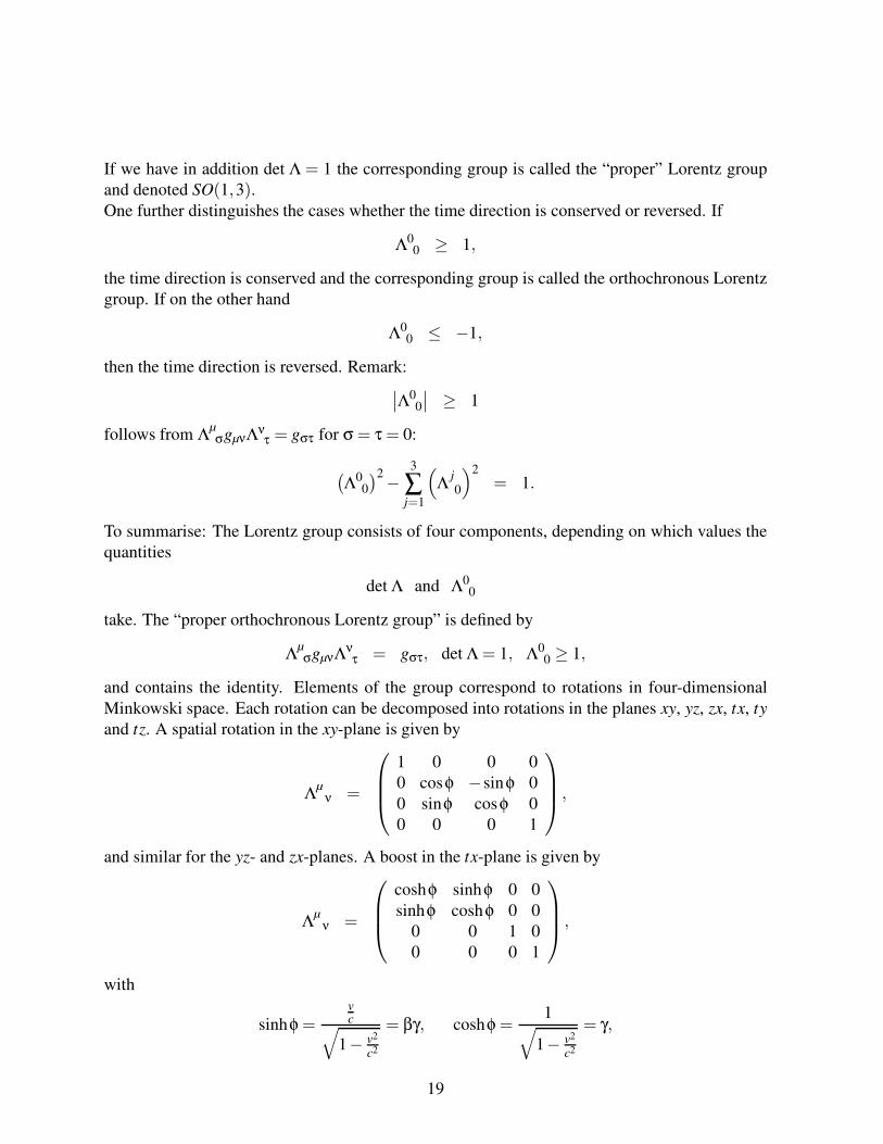
and contains the identity. Elements of the group correspond to rotations in four-dimensional
Minkowski space. Each rotation can be decomposed into rotations in the planes xy, yz, zx, tx, ty
and tz. A spatial rotation in the xy-plane is given by
Λµ
ν =
1 0 0 0
0 cosφ −sinφ 0
0 sinφ cosφ 0
0 0 0 1
,
and similar for the yz- and zx-planes. A boost in the tx-plane is given by
Λµ
ν =
coshφ sinhφ 0 0
sinhφ coshφ 0 0
0 0 1 0
0 0 0 1
,
with
sinhφ =vc
√
1− v2
c2
= βγ, coshφ =1
√
1− v2
c2
= γ,
19
where we used the standard abreviations
β =v
c, γ =
1√
1− v2
c2
.
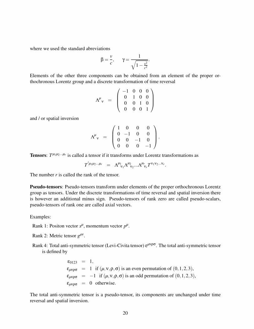
Elements of the other three components can be obtained from an element of the proper or-
thochronous Lorentz group and a discrete transformation of time reversal
Λµ
ν =
−1 0 0 0
0 1 0 0
0 0 1 0
0 0 0 1
and / or spatial inversion
Λµ
ν =
1 0 0 0
0 −1 0 0
0 0 −1 0
0 0 0 −1
.
Tensors: T µ1µ2...µr is called a tensor if it transforms under Lorentz transformations as
T′µ1µ2...µr = Λ
µ1ν1
Λµ2
ν2...Λ
µrνr
T ν1ν2...νr .
The number r is called the rank of the tensor.
Pseudo-tensors: Pseudo-tensors transform under elements of the proper orthochronous Lorentz
group as tensors. Under the discrete transformations of time reversal and spatial inversion there
is however an additional minus sign. Pseudo-tensors of rank zero are called pseudo-scalars,
pseudo-tensors of rank one are called axial vectors.
Examples:
Rank 1: Positon vector xµ, momentum vector pµ.
Rank 2: Metric tensor gµν.
Rank 4: Total anti-symmetric tensor (Levi-Civita tensor) εµνρσ. The total anti-symmetric tensor
is defined by
ε0123 = 1,
εµνρσ = 1 if (µ,ν,ρ,σ) is an even permutation of (0,1,2,3),
εµνρσ = −1 if (µ,ν,ρ,σ) is an odd permutation of (0,1,2,3),
εµνρσ = 0 otherwise.
The total anti-symmetric tensor is a pseudo-tensor, its components are unchanged under time
reversal and spatial inversion.
20
3.3 The Poincaré group
The Poincaré group consists of elements of the Lorentz group and translations. The group ele-
ments act on four vectors according to the following transformation law :
x′µ = Λ
µν xν +aµ.
Λ describes rotations in four dimensional space-time (e.g. ordinary rotations on the spacial
components plus boosts) whereas a describes translations.
The group multiplication law is given by
a1,Λ1a2,Λ2 = a1 +Λ1a2,Λ1Λ2.
The generators of the Poincaré group can be realised as differential operators :
Pµ = i∂µ,
Mµν = i(xµ∂ν− xν∂µ
).
The algebra of the Poincaré group is given by
[Mµν,Mρσ
]= −i
(gµρMνσ−gνρMµσ +gµσMρν−gνσMρµ
),
[Mµν,Pσ
]= i
(gνσPµ−gµσPν
),
[Pµ,Pν
]= 0.
The Poincaré algebra is a Lie algebra, but it is not semi-simple, since it has an Abelian non-trivial
ideal (Pµ).Casimir operators are M2 and W 2 where
M2 = PµPµ, W µ =1
2εµνρσPνMρσ.
W µ is called the Lubanski-Pauli vector.
21
4 Review of classical field theory
4.1 The action principle
From classical mechanics we are familiar with Hamilton’s principle of the least action for sys-
tems with a finite number of degrees of freedom. This principle generalises to systems with
infinite many degrees of freedom:
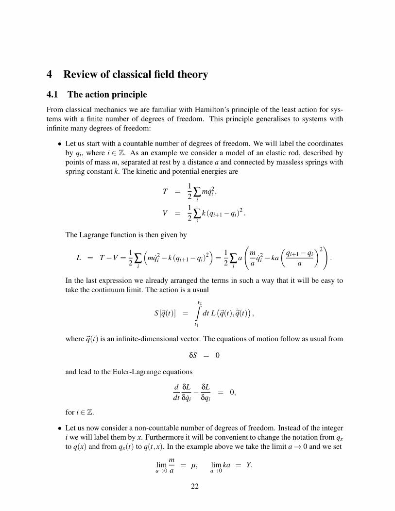
• Let us start with a countable number of degrees of freedom. We will label the coordinates
by qi, where i ∈ Z. As an example we consider a model of an elastic rod, described by
points of mass m, separated at rest by a distance a and connected by massless springs with
spring constant k. The kinetic and potential energies are
T =1
2∑
i
mq2i ,
V =1
2∑
i
k (qi+1−qi)2 .
The Lagrange function is then given by
L = T −V =1
2∑
i
(
mq2i − k (qi+1−qi)
2)
=1
2∑
i
a
(
m
aq2
i − ka
(qi+1−qi
a
)2)
.
In the last expression we already arranged the terms in such a way that it will be easy to
take the continuum limit. The action is a usual
S [~q(t)] =
t2∫
t1
dt L(~q(t),~q(t)
),
where~q(t) is an infinite-dimensional vector. The equations of motion follow as usual from
δS = 0
and lead to the Euler-Lagrange equations
d
dt
δL
δqi
− δL
δqi
= 0,
for i ∈ Z.
• Let us now consider a non-countable number of degrees of freedom. Instead of the integer
i we will label them by x. Furthermore it will be convenient to change the notation from qx
to q(x) and from qx(t) to q(t,x). In the example above we take the limit a→ 0 and we set
lima→0
m
a= µ, lim
a→0ka = Y.
22

Furthermore the expression (qi+1−qi)/a becomes in the continuum limit
lima→0
q(t,x+a)−q(t,x)
a=
∂q(t,x)
∂x.
We obtain for the Lagrange function
L =1
2
∞∫
−∞
dx
[
µ
(∂q(t,x)
∂t
)2
−Y
(∂q(t,x)
∂x
)2]
.
The expression
L =1
2
[
µ
(∂q(t,x)
∂t
)2
−Y
(∂q(t,x)
∂x
)2]
is called the Lagrange density or Lagrangian. The action is given by
S =
t2∫
t1
dt
∞∫
−∞
dx L .
We may view q(t,x) as a classical field in a (1+ 1)-dimensional space-time. Note that
the Lagrange density is a function of the time derivative ∂q/∂t and the spatial derivative
∂q/∂x.
We now consider the generalisation to four-dimensional space-time. We assume that the La-
grange density is a function of the field ψ(x) and its first derivative ∂µψ(x):
L(ψ(x),∂µψ(x)
).
The motivation is as follows: Classical mechanics suggests to include a dependence on ψ(x) and
the time derivative ∂0ψ(x). Lorentz invariance instructs us not to single out a specific direction
in space-time. We therefore allow a dependence on all first derivatives ∂µψ(x). In principle we
could include also second or higher derivatives, however for our purpose it will be sufficient to
restrict us to first derivatives. The action is given by
S =
t2∫
t1
dt
∫d3x L =
1
c
∫d4x L .
From the principle of least action
δS = 0,
23
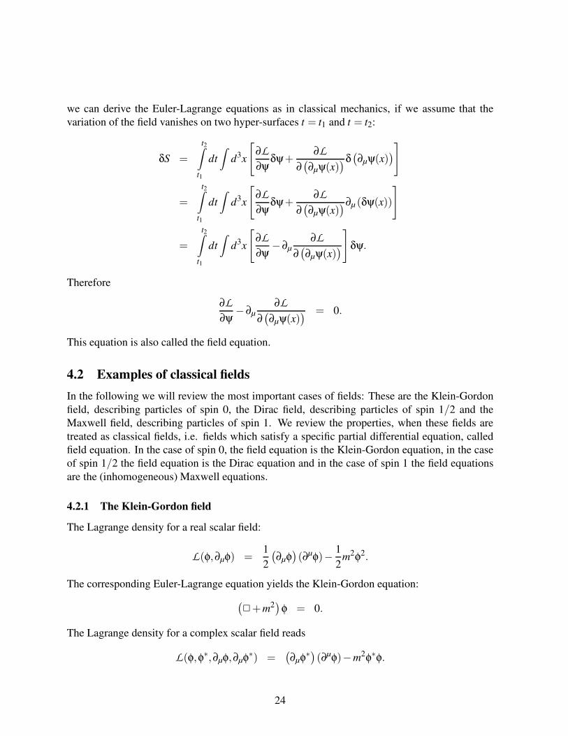
we can derive the Euler-Lagrange equations as in classical mechanics, if we assume that the
variation of the field vanishes on two hyper-surfaces t = t1 and t = t2:
δS =
t2∫
t1
dt
∫d3x
[
∂L
∂ψδψ+
∂L
∂(∂µψ(x)
)δ(∂µψ(x)
)
]
=
t2∫
t1
dt
∫d3x
[
∂L
∂ψδψ+
∂L
∂(∂µψ(x)
)∂µ (δψ(x))
]
=
t2∫
t1
dt
∫d3x
[
∂L
∂ψ−∂µ
∂L
∂(∂µψ(x)
)
]
δψ.
Therefore
∂L
∂ψ−∂µ
∂L
∂(∂µψ(x)
) = 0.
This equation is also called the field equation.
4.2 Examples of classical fields
In the following we will review the most important cases of fields: These are the Klein-Gordon
field, describing particles of spin 0, the Dirac field, describing particles of spin 1/2 and the
Maxwell field, describing particles of spin 1. We review the properties, when these fields are
treated as classical fields, i.e. fields which satisfy a specific partial differential equation, called
field equation. In the case of spin 0, the field equation is the Klein-Gordon equation, in the case
of spin 1/2 the field equation is the Dirac equation and in the case of spin 1 the field equations
are the (inhomogeneous) Maxwell equations.
4.2.1 The Klein-Gordon field
The Lagrange density for a real scalar field:
L(φ,∂µφ) =1
2
(∂µφ)(∂µφ)− 1
2m2φ2.
The corresponding Euler-Lagrange equation yields the Klein-Gordon equation:
(+m2
)φ = 0.
The Lagrange density for a complex scalar field reads
L(φ,φ∗,∂µφ,∂µφ∗) =(∂µφ∗
)(∂µφ)−m2φ∗φ.
24

In the complex case we treat φ and φ∗ as two independent fields. Variation with respect to φ∗
yields(+m2
)φ = 0,
variation with respect to φ gives(+m2
)φ∗ = 0.
4.2.2 The Dirac field
Although Dirac spinors are associated with the quantum mechanical description of spin, we may
ignore this fact for the moment and simply take a Dirac spinor as a four-component vector with
complex entries. A Dirac field associates to every space-time point x a four-component spinor
ψα(x), where α takes the values α ∈ 1,2,3,4. Note that α is not a Lorentz index, it is a Dirac
index. (We use greek letters from the beginning of the greek alphabet for spinor indices and
greek letters from the middle of the greek alphabet for Lorentz indices.)
Let us define the Dirac matrices. These are (4×4)-matrices, which satisfy the anti-commutation
rules
γµ,γν = 2gµν1.
(The anti-commutator of two matrices is A,B= AB+BA.) In addition, there is a fifth matrix
γ5, defined by
γ5 = iγ0γ1γ2γ3 =i
24εµνρσγµγνγργσ,
which satisfies
γµ,γ5= 0.
There are various representations for the Dirac matrices, a convenient choice is the Weyl repre-
sentation. In order to define the Weyl representation we first recall the Pauli matrices. These are
2×2-matrices, given by
σx =
(0 1
1 0
)
, σy =
(0 −i
i 0
)
, σz =
(1 0
0 −1
)
.
We write~σ = (σx,σy,σz). Next, we define the 4-dimensional σµ-matrices (and σµ-matrices):
σµ
AB= (1,−~σ) , σµAB = (1,~σ) .
Here 1 denotes the 2×2-identity matrix. There are four 2×2-matrices σ0AB
, σ1AB
, σ2AB
and σ3AB
.
The indices A and B take values A, B ∈ 1,2. Analog statements hold for σµAB. We are now in
a position to give the Weyl representation for the Dirac matrices:
γµ =
(0 σµ
σµ 0
)
, γ5 = iγ0γ1γ2γ3 =
(1 0
0 −1
)
.
25
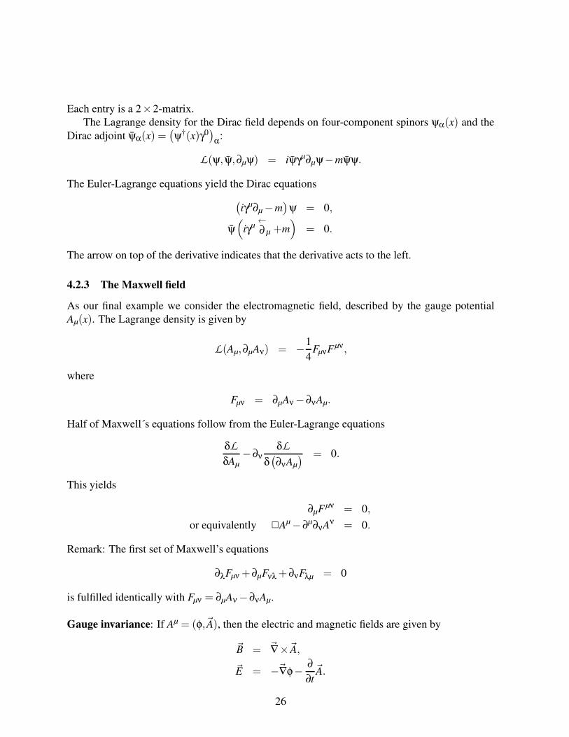
Each entry is a 2×2-matrix.
The Lagrange density for the Dirac field depends on four-component spinors ψα(x) and the
Dirac adjoint ψα(x) =(ψ†(x)γ0
)
α:
L(ψ, ψ,∂µψ) = iψγµ∂µψ−mψψ.
The Euler-Lagrange equations yield the Dirac equations
(iγµ∂µ−m
)ψ = 0,
ψ(
iγµ←∂ µ +m
)
= 0.
The arrow on top of the derivative indicates that the derivative acts to the left.
4.2.3 The Maxwell field
As our final example we consider the electromagnetic field, described by the gauge potential
Aµ(x). The Lagrange density is given by
L(Aµ,∂µAν) = −1
4FµνFµν,
where
Fµν = ∂µAν−∂νAµ.
Half of Maxwell´s equations follow from the Euler-Lagrange equations
δL
δAµ
−∂νδL
δ(∂νAµ
) = 0.
This yields
∂µFµν = 0,
or equivalently Aµ−∂µ∂νAν = 0.
Remark: The first set of Maxwell’s equations
∂λFµν +∂µFνλ +∂νFλµ = 0
is fulfilled identically with Fµν = ∂µAν−∂νAµ.
Gauge invariance: If Aµ = (φ,~A), then the electric and magnetic fields are given by
~B = ~∇×~A,~E = −~∇φ− ∂
∂t~A.
26
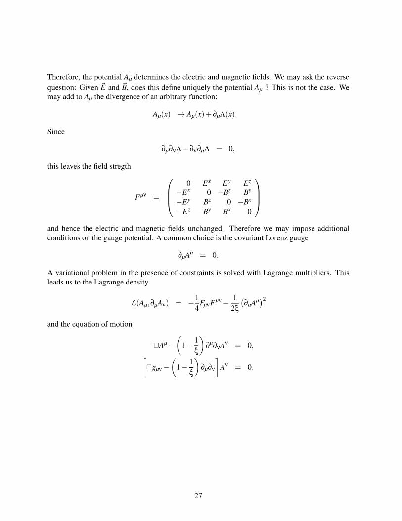
Therefore, the potential Aµ determines the electric and magnetic fields. We may ask the reverse
question: Given ~E and ~B, does this define uniquely the potential Aµ ? This is not the case. We
may add to Aµ the divergence of an arbitrary function:
Aµ(x) → Aµ(x)+∂µΛ(x).
Since
∂µ∂νΛ−∂ν∂µΛ = 0,
this leaves the field stregth
Fµν =
0 Ex Ey Ez
−Ex 0 −Bz By
−Ey Bz 0 −Bx
−Ez −By Bx 0
and hence the electric and magnetic fields unchanged. Therefore we may impose additional
conditions on the gauge potential. A common choice is the covariant Lorenz gauge
∂µAµ = 0.
A variational problem in the presence of constraints is solved with Lagrange multipliers. This
leads us to the Lagrange density
L(Aµ,∂µAν) = −1
4FµνFµν− 1
2ξ
(∂µAµ
)2
and the equation of motion
Aµ−(
1− 1
ξ
)
∂µ∂νAν = 0,
[
gµν−(
1− 1
ξ
)
∂µ∂ν
]
Aν = 0.
27
5 Quantum field theory: The canonical formalism
There are several approaches to quantum field theory. In this course we will focus on two of
them: The canonical formalism and the path integral formalism. We start with the canonical
formalism.
Within the canonical approach a system is described by a state vector and operators acting
on the state vectors. An important operator will be the Hamilton operator (or Hamiltonian).
The Hamilton operator can be obtained by analogy with classical field theory. In classical field
theory we have a Hamilton density, consisting of the fields and derivatives of the fields. Promot-
ing the fields to operators gives us the Hamilton operator of quantum field theory.
Within the Schrödinger picture, the time evolution of a state is governed by the Hamilton
operator. We will also consider the Heisenberg picture, where the time-dependence is carried
by the operators, while the states are time-independent. Finally, a third picture will be useful for
practical calculations: the interaction picture.
Remark: Classical physics is concerned with classical point-like particles and classical fields.
In quantum mechanics we describe particles by a wave function. This is often called “first quan-
tisation”. If fields are present, they are treated classically. We would like to treat (matter) par-
ticles and (force) fields, which also have a particle nature, on equal footing. This is achieved
in quantum field theory, where fields are described by operators. This is often called “second
quantisation”. However we should add a warning here: The expression “second quantisation”
might give wrong allusions. Also in quantum field theory we quantise only once. In fact we will
soon see that we may treat a quantum field as a collection of infinite many harmonic oscillators.
Each harmonic oscillator is quantised as in quantum mechanics.
5.1 The Klein-Gordon field as harmonic oscillators
We start with the simplest example, a real scalar field as a classical field with Lagrange density
L(φ,∂µφ) =1
2
(∂µφ)(∂µφ)− 1
2m2φ2.
We define the canonical conjugated momentum field by
π(x) =∂L
∂φ(x).
For the Klein-Gordon field we find
π(x) = φ(x).
The Hamilton function is given by
H =
∫d3x[π(x)φ(x)−L
]=
∫d3x
[1
2π2 +
1
2
(~∇φ)2
+1
2m2φ2
]
.
28
We write
H =
∫d3x H , H = π(x)φ(x)−L =
1
2π2 +
1
2
(~∇φ)2
+1
2m2φ2.
H is called the Hamiltonian. The energy-momentum tensor is given by
T µν =∂L
∂(∂µφ)∂νφ−gµνL = (∂µφ)(∂νφ)− 1
2gµν(∂ρφ)(∂ρφ)+
1
2gµνm2φ2
If the Lagrange density does not depend explicitly on x, i.e. the x-dependence is only through
φ(x), then Noether’s theorem implies
∂µT µν = 0.
The four “conserved charges” are
H =
∫d3x T 00 =
∫d3x H
and
Pi =∫
d3x T 0i =−∫
d3x π∂iφ.
The quantity
−π~∇φ
is called the momentum density and
~P = −∫
d3x π~∇φ
the total momentum of the classical field.
Please note the difference between the canonical conjugated momentum field π(x) and the mo-
mentum density [−π(x)~∇φ(x)]. These are not equal. This can already be seen by the fact that the
former is a scalar quantity, wheras the latter is vector-valued.
Let us write the classical Klein-Gordon field as a Fourier integral with respect to~x:
φ(t,~x) =∫
d3p
(2π)3ei~p·~xφ(t,~p).
Then the Klein-Gordon equation becomes
[∂2
∂t2+(
|~p|2 +m2)]
φ(t,~p) = 0.
29
This is the same as the equation of a harmonic oscillator with frequency
ω~p =
√
|~p|2 +m2.
For a harmonic oscillator we know how to make the transition from the classical picture to the
quantum world. The Hamilton operator for a quantum-mechanical harmonic osciallator with this
frequency is given by
H =1
2π2~p +
1
2ω2~pφ2
~p.
The corresponding creation and annihilation operators are
a~p =
√ω~p
2φ~p +
i√
2ω~pπ~p, a
†~p =
√ω~p
2φ~p−
i√
2ω~pπ~p.
We may solve these equations for φ~p and π~p and obtain
φ~p =1
√2ω~p
(
a~p + a†~p
)
, π~p =−i
√ω~p
2
(
a~p− a†~p
)
.
Note that the operators φ~p and π~p correspond to a single momentum mode ~p.
5.2 The Schrödinger picture
We are now in a position to present a quantum field as an operator. The basic idea is to take a
linear superposition of momentum modes, where each individual momentum mode behaves like
a quantum mechanical harmonic oscillator.
We start with the Schrödinger picture, where the operators do not depend on time. In the
Schrödinger picture we denote operators by O(~x), or OS(~x), if we want to emphasize that an
operator refers to the Schrödinger picture. In the Schrödinger picture, operators may depend on
the spatial coordinates~x, but not on the time coordinate t.
In the Schrödinger picture the time dependence is carried by the states. States are denoted by
|X〉. If we want to emphasize that the states carry the time-dependence we will write |X , t〉. If we
further want to emphasize that a state refers to the Schrödinger picture we will put a subscript S
and write |X , t〉S.
We start from
[qi, p j
]= iδi j,
[qi, q j
]=
[pi, p j
]= 0,
which for a continous system becomes
[φ(~x), π(~y)
]= iδ3(~x−~y),
[φ(~x), φ(~y)
]= [π(~x), π(~y)] = 0.
30
These are called the canonical commutation relations. We write a Fourier representation for
the fields:
φ(~x) =∫
d3 p
(2π)3
1√
2ω~p
(
a~pei~p·~x + a†~pe−i~p·~x
)
,
π(~x) =∫
d3 p
(2π)3(−i)
√ω~p
2
(
a~pei~p·~x− a†~pe−i~p·~x
)
.
Note that we are considering a real field. Therefore we would like to have that φ(~x) is self-adjoint:
(φ(~x)
)†= φ(~x).
In addition we would like to have
(
a†)†
= a.
These two conditions explain the sign in the exponent e−i~p·~x in the term proportional to a†~p in the
Fourier representation of φ(~x). The inverse formulae read
a~p =∫
d3x
(√ω~p
2φ(~x)+
i√
2ω~pπ(~x)
)
e−i~p·~x,
a†~p =
∫d3x
(√ω~p
2φ(~x)− i
√2ω~p
π(~x)
)
ei~p·~x.
The commutation relation becomes[
a~p, a†~q
]
= (2π)3δ3(~p−~q).
In detail:
[
a~p, a†~q
]
=
[∫d3x
(√ω~p
2φ(~x)+
i√
2ω~pπ(~x)
)
e−i~p·~x,∫
d3y
(√ω~q
2φ(~y)− i
√2ω~q
π(~y)
)
ei~q·~y]
=
∫d3x
∫d3ye−i~p·~xei~q·~y
(
− i
2
√
ω~p
ω~q
[φ(~x), π(~y)
]+
i
2
√
ω~q
ω~p
[π(~x), φ(~y)
]
)
=
∫d3x
∫d3ye−i~p·~xei~q·~y
(
1
2
√
ω~p
ω~q+
1
2
√
ω~q
ω~p
)
δ3(~x−~y)
=1
2
(√
ω~p
ω~q+
√
ω~q
ω~p
)∫d3xe−i(~p−~q)·~x
=1
2
(√
ω~p
ω~q+
√
ω~q
ω~p
)
(2π)3δ3(~p−~q) = (2π)3δ3(~p−~q).
31

The remaining commutation relations for the creation and annihilation operators are
[a~p, a~q
]=[
a†~p, a
†~q
]
= 0.
Let us summarise: The equivalence of the canonical commutation relations
[φ(~x), π(~y)
]= iδ3(~x−~y),
[φ(~x), φ(~y)
]= [π(~x), π(~y)] = 0
in momentum space are the relations
[
a~p, a†~q
]
= (2π)3δ3(~p−~q),[a~p, a~q
]=[
a†~p, a
†~q
]
= 0.
The Hamiltonian becomes
H =
∫d3x
[1
2π2 +
1
2
(~∇φ)2
+1
2m2φ2
]
=
∫d3p
(2π)3ω~p
(
a†~pa~p +
1
2
[
a~p, a†~p
])
The second term is proportional to δ3(~0) and gives an infinite constant. Such a term can be
expected: A single harmonic oscillator has the ground state energy 12ω, summing over an infinite
number of harmonic oscillators yields an infinite ground state energy. As experiments can only
measure energy differences from the ground state, we will ignore this term. Expressing the
Hamiltonian in terms of annihilation and creation operators we will encounter at intermediate
stages expressions proportional to a~pa~p and a†~pa
†~p. These expressions are in addition proportional
to ω2~p−|~p|2−m2 = 0 and vanish therefore.
The commutation relations of the Hamiltonian with the annihilation and creation operators
are[
H, a†~q
]
= ω~qa†~q,
[H, a~q
]= −ω~qa~q.
Let us look at the total momentum operator
~P = −∫
d3x π(~x)~∇φ(~x) =∫
d3 p
(2π)3~p
(
a†~pa~p +
1
2
[
a~p, a†~p
])
.
Again, the second term will give a contribution proportional to δ3(~0), which we will ignore. In
order to show the equality for the last equal sign in the equation above, we will encounter the
following integrals:
∫d3p
(2π)3~p a~p a−~p and
∫d3 p
(2π)3~p a
†~p a
†−~p.
The integrands of these integrals are anti-symmetric under ~p→−~p. Therefore these integrals
vanish. With the same reasoning one can argue that ~pδ3(~0) is anti-symmetric under ~p→−~p and
therefore the infinite constant has to vanish after integration over d3 p.
32

Let us look at the commutation relations of ~P with a†~q and a~q. We have
[
~P, a†~q
]
=∫
d3p
(2π)3~p(
a†~pa~pa
†~q− a
†~qa
†~pa~p
)
=∫
d3 p
(2π)3~pa
†~p
[
a~p, a†~q
]
=∫
d3p
(2π)3~pa
†~p (2π)3 δ3 (~p−~q) = ~qa
†~q.
A similar relation (with an additional minus sign) holds for a~q. Thus we have
[
~P, a†~q
]
= ~qa†~q,
[
~P, a~q
]
= −~qa~q.
We may combine the Hamilton operator H and the three-momentum operator ~P into a four-
momentum operator Pµ:
Pµ =(
H, ~P)
=∫
d3 p
(2π)3pµ
(
a†~pa~p +
1
2
[
a~p, a†~p
])
,
with pµ = (ω~p,~p) and ω~p =√
|~p|2 +m2. From now on we will write
E~p = ω~p =+
√
|~p|2 +m2
Note that the energy is always positive. We have
[
Pµ, a†~q
]
= qµa†~q,
[Pµ, a~q
]= −qµa~q.
Let us now discuss the states. The ground state is defined as the state, which is annihilated by
all annihilation operators. We denote the ground state by |0〉. Thus
a~p |0〉 = 0 for all a~p.
If we drop the infinite constant above, the ground state has energy E = 0 and momentum ~p = 0.
All other states can be obtained by acting on |0〉 with creation operators. As a first example let
us consider the state a†~p|0〉. We have
Pµ(
a†~q |0〉
)
=(
a†~qPµ +
[
Pµ, a†~q
])
|0〉 = qµ(
a†~q |0〉
)
.
Thus, a†~p|0〉 is an eigenstate of Pµ with momentum ~p and energy E~p =
√
|~p|2 +m2. The state
a†~p|0〉 is called a one-particle state.
Next, consider the state
a†~p1
a†~p2|0〉.
33
This state is again an eigenstate of Pµ with momentum ~p1 +~p2 and energy E~p1+E~p2
. The state
a†~p1
a†~p2|0〉 is called a two-particle state. Further note that
a†~p1
a†~p2|0〉 = a
†~p2
a†~p1|0〉,
since a†~p1
and a†~p2
commute.
Following this pattern we can construct n-particle states as
a†~p1
a†~p2...a†
~pn|0〉
and therefore the full spectrum of the Hamilton operator.
Summary: The spectrum of the Hamilton operator
H = =
∫d3x
[1
2π2 +
1
2
(~∇φ)2
+1
2m2φ2
]
is obtained from the ground state |0〉 by successively applying creation operators a†~p. All states
are reached this way.
Normalisation: For the ground state we choose the normalisation
〈0|0〉 = 1.
For one-particle state we choose the normalisation
〈~p|~q〉 = 2E~p(2π)3δ3 (~p−~q) .
Therefore
|~p〉 =√
2E~pa†~p |0〉 .
Remark: This normalisation is Lorentz invariant. Consider the boost
E ′ = γE−βγp3,
p′3 = −βγE + γp3.
From
δ( f (x)− f (x0)) =1
| f ′(x0)|δ(x− x0)
it follows that
δ3(~p−~q) = δ3(~p′−~q′) · dp′3dp3
= δ3(~p′−~q′)γ(
1−βdE
dp3
)
= δ3(~p′−~q′)γ(
1−βp3
E
)
= δ3(~p′−~q′)E ′
E.
34
Remark: ∫d3p
(2π)3
1
2E~p=
∫d4 p
(2π)4(2π)δ(p2−m2)θ(p0)
is a Lorentz-invariant 3-momentum integral. Therefore, if f (p) is Lorentz-invariant, so is∫
d3p
(2π)3
1
2E~pf (p).
The normalisation of the n-particle state is
|~p1,~p2, ...,~pn〉 =√
2E~p1·2E~p2
· ... ·2E~pna
†~p1
a†~p2...a†
~pn|0〉 .
Since a creation operator commutes with any other creation operator, it does not matter in which
order we write the creation operators. In order to have a manifest symmetric expressions we can
equally well write
|~p1,~p2, ...,~pn〉 =√
2E~p1·2E~p2
· ... ·2E~pn
1
n!∑
σ∈Sn
a†~pσ1
a†~pσ2
...a†~pσn|0〉 ,
where the sum is over n! permutations of the set 1,2, ...,n.
5.3 The Fock space
We have already mentioned, that all states of the system can be reached by succesively applying
creation operators a†~p to the ground state |0〉. We can formalise this situation. From quantum
mechanics we are familiar with the concept of a Hilbert space. We recall that a Hilbert space is
a vectorspace, which has an inner product and which is complete. As base field we will always
taks the complex numbers C. Let us denote by V1 the Hilbert space of the one-particle states
V1 =|~p〉 | ~p ∈ R
3.
For convenience we denote
V0 = C.
We further set
Vn = Sym (V1)⊗n ,
i.e. Vn is the symmetrised n-fold tensor product of V1. Symmetrisation means for example that
|~p1〉⊗ |~p2〉 and |~p2〉⊗ |~p1〉 are identified in V2 and we simply write
|~p1,~p2〉 = |~p1〉⊗sym |~p2〉 = |~p2〉⊗sym |~p1〉 ∈ V2.
The Fock space of the system is the direct sum of all Vn, where n ∈ N0.
V =∞⊕
n=0
Vn
= V0⊕V1⊕V2⊕ ...
The Fock space is a Hilbert space. V0 contains the zero-particle states, V1 the one-particles state,
V2 the two-particle states, etc.. Thus the states of our system form a Fock space.
35
5.4 The Heisenberg picture
We now turn to the Heisenberg picture. In this section we will denote for clarity operators in the
Heisenberg picture by OH(x) and operators in the Schrödinger picture by OS(~x). In later section
we will drop the subscripts H and S and denote the operators in the Heisenberg picture simply
by O(x) and the operators in the Schrödinger picture by O(~x). Note that the operators in the
Heisenberg picture depend on the four-vector x, while the operators in the Schrödinger picture
depend only on the spatial vector~x, therefore it is clear what operator is meant.
In the Heisenberg picture, the operators φH(x) and πH(x) are now time-dependent:
φH(x) = eiHt φS(~x)e−iHt ,
πH(x) = eiHt πS(~x)e−iHt .
If the Hamilton operator is time-independent we have HH = HS = H. Furthermore we have
T exp
−i
t∫
0
dt ′H
= e−iHt .
The states in the Heisenberg picture are given by
|X〉H = eiHt |X , t〉S .
At t = 0 the states in the Heisenberg picture and the Schrödinger picture agree: |X〉H = |X ,0〉S.
Sometimes it is useful to generalise this slightly , such that the states in the Heisenberg picture
and the Schrödinger picture agree at t0. The transformation formulae in this case read
OH (x) = eiH(t−t0)OS(~x)e−iH(t−t0), |X〉H = eiH(t−t0) |X , t〉S .
Note that the Heisenberg operator OH depends in this case on t and t0 (to be concrete: OH
depends on the difference t− t0) and that the Heisenberg state |X〉H is always independent of t:
i∂
∂t|X〉H = 0.
From the Heisenberg equation of motion
i∂
∂tOH =
[OH , H
],
we find
i∂
∂tφH(x) = iπH(x),
i∂
∂tπH(x) = i
(~∇2−m2
)
φH(x).
36
Combining these two results yields
∂2
∂t2φH(x) =
(~∇2−m2
)
φH(x),
or(+m2
)φH(x) = 0.
Thus, the operator φH(x) fulfills the Klein-Gordon equation.
For a better understanding we express φH(x) and πH(x) in terms of creation and annihilation
operators. From[
H, a†~p
]
= E~p a†~p,
[H, a~p
]= −E~p a~p,
we have
Ha†~p = a
†~p
(H +E~p
), Ha~p = a~p
(H−E~p
),
and therefore
Hna†~p = a
†~p
(H +E~p
)n, Hna~p = a~p
(H−E~p
)n.
Therefore
eiHt a†~pe−iHt = a
†~peiE~pt , eiHt a~pe−iHt = a~pe−iE~pt .
From
φS(~x) =∫
d3 p
(2π)3
1√
2E~p
(
a~pei~p·~x + a†~pe−i~p·~x
)
,
πS(~x) =∫
d3 p
(2π)3(−i)
√
E~p
2
(
a~pei~p·~x− a†~pe−i~p·~x
)
we then obtain
φH(x) =∫
d3 p
(2π)3
1√
2E~p
(
a~pe−ip·x + a†~peip·x
)∣∣∣
p0=E~p
,
πH(x) =∂
∂tφH(x).
Remark: a~p and a†~p denote always the time-independent Schrödinger-picture ladder operators.
The time-dependent ladder operators in the Heisenberg picture are
a†~p,H(t) = eiHt a
†~pe−iHt = a
†~peiE~pt , a~p,H(t) = eiHt a~pe−iHt = a~pe−iE~pt .
The subscript H indicates Heisenberg operators.
Remark 2: The above equation makes the duality between particle and wave interpretations of
the quantum field explicit: On the one hand, φH(x) is written as a Hilbert space operator, which
creates and destroys the particles that are the quanta of the field excitations. On the other hand,
φH(x) is written as a linear combination of plane-wave solutions of the Klein-Gordon equation.
37
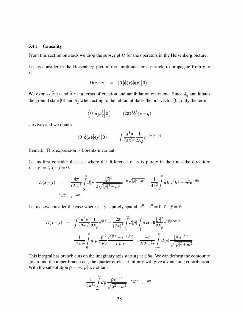
5.4.1 Causality
From this section onwards we drop the subscript H for the operators in the Heisenberg picture.
Let us consider in the Heisenberg picture the amplitude for a particle to propagate from y to
x:
D(x− y) =⟨0∣∣φ(x)φ(y)
∣∣0⟩.
We express φ(x) and φ(y) in terms of creation and annihilation operators. Since a~q annihilates
the ground state |0〉 and a†~p when acting to the left annihilates the bra-vector 〈0|, only the term
⟨
0
∣∣∣a~pa
†~q
∣∣∣0⟩
= (2π)3δ3(~p−~q)
survives and we obtain
⟨0∣∣φ(x)φ(y)
∣∣0⟩
=
∫d3p
(2π)3
1
2E~pe−ip·(x−y)
Remark: This expression is Lorentz-invariant.
Let us first consider the case where the difference x− y is purely in the time-like direction:
x0− y0 = t,~x−~y = 0:
D(x− y) =4π
(2π)3
∞∫
0
d|~p| |~p|2
2√
|~p|2 +m2e−it√|~p|2+m2
=1
4π2
∞∫
m
dE√
E2−m2e−iEt
t→∞∼ e−imt .
Let us now consider the case where x− y is purely spatial: x0− y0 = 0,~x−~y =~r:
D(x− y) =∫
d3 p
(2π)3
1
2E~pei~p·~r =
2π
(2π)3
∞∫
0
d|~p|1∫
−1
d cosθ|~p|22E~p
ei|~p|r cosθ
=1
(2π)2
∞∫
0
d|~p| |~p|2
2E~p
ei|~p|r− e−i|~p|r
i|~p|r =−i
2(2π)2r
∞∫
−∞
d|~p| |~p|ei|~p|r
√
|~p|2 +m2
This integral has branch cuts on the imaginary axis starting at±im. We can deform the contour to
go around the upper branch cut, the quarter circles at infinity will give a vanishing contribution.
With the substitution ρ =−i|~p| we obtain
1
4π2r
∞∫
m
dρρe−ρr
√
ρ2−m2
r→∞∼ e−mr.
38
We find that the propagation amplitude for space-like distances is exponentially vanishing, but
non-zero. Is this a problem with causality ? No, to discuss causality we should not ask whether
particles can propagate over space-like distances, but whether a measurement performed at one
point can affect a measurement at another point whose separation from the first is space-like. The
simplest thing to measure is the field φ(x), so let’s have a look at the commutator [φ(x), φ(y)], if
this commutator vanishes for space-like distances, one measurement cannot affect another one
separated at a space-like distance.
[φ(x), φ(y)
]=
∫d3 p
(2π)3
1√
2E~p
∫d3q
(2π)3
1√
2E~q
[(
a~pe−ip·x + a†~peip·x
)
,(
a~qe−iq·y + a†~qeiq·y
)]
=
∫d3 p
(2π)3
1
2E~p
(
e−ip·(x−y)− eip·(x−y))
= D(x− y)−D(y− x).
When (x− y)2 < 0, we can perform a Lorentz-transformation on the second term (since each
term is separately Lorentz-invariant), taking
(x− y)→−(x− y).
The two terms are therefore equal and cancel in the sum. Therefore causality is preserved.
Remark: If (x− y)2 > 0 there is no continuous Lorentz-transformation, which takes (x− y)→−(x− y).
5.4.2 The Klein-Gordon propagator
Let us study the commutator [φ(x), φ(y)] a little bit further. Since it is a c-number, we have
[φ(x), φ(y)
]=
⟨0∣∣[φ(x), φ(y)
]∣∣0⟩.
Let us assume that x0 > y0. Then we have
⟨0∣∣[φ(x), φ(y)
]∣∣0⟩
=
∫d3p
(2π)3
1
2E~p
(
e−ip·(x−y)− eip·(x−y))
=∫
d3p
(2π)3
1
2E~pe−ip·(x−y)
∣∣∣∣
p0=E~p
+1
−2E~pe−ip·(x−y)
∣∣∣∣
p0=−E~p
=∫
d3p
(2π)3
∫dp0
2πi
−1
p2−m2e−ip·(x−y).
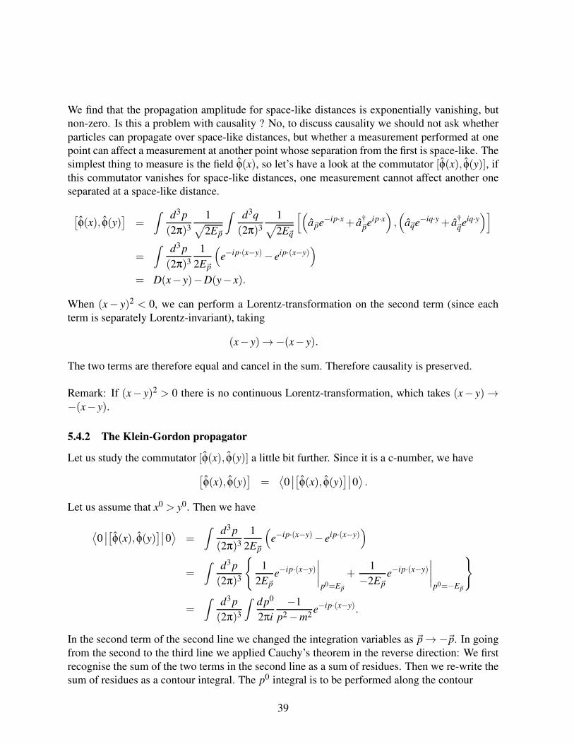
In the second term of the second line we changed the integration variables as ~p→−~p. In going
from the second to the third line we applied Cauchy’s theorem in the reverse direction: We first
recognise the sum of the two terms in the second line as a sum of residues. Then we re-write the
sum of residues as a contour integral. The p0 integral is to be performed along the contour
39
Re(p0)
Im(p0)
−E~p E~p
The condition x0 > y0 ensures that the half-circle at infinity in the lower complex plane gives a
vanishing contribution. To keep track of the contour we also write
⟨0∣∣[φ(x), φ(y)
]∣∣0⟩
=
∫d3 p
(2π)3
∫dp0
2π
i
(p0 + iε)2−|~p|2−m2
e−ip·(x−y),
where ε is an infinitessimal quantity with ε > 0. We define
DR(x− y) = θ(x0− y0)⟨0∣∣[φ(x), φ(y)
]∣∣0⟩=
∫d4p
(2π)4
i
(p0 + iε)2−|~p|2−m2
e−ip·(x−y).
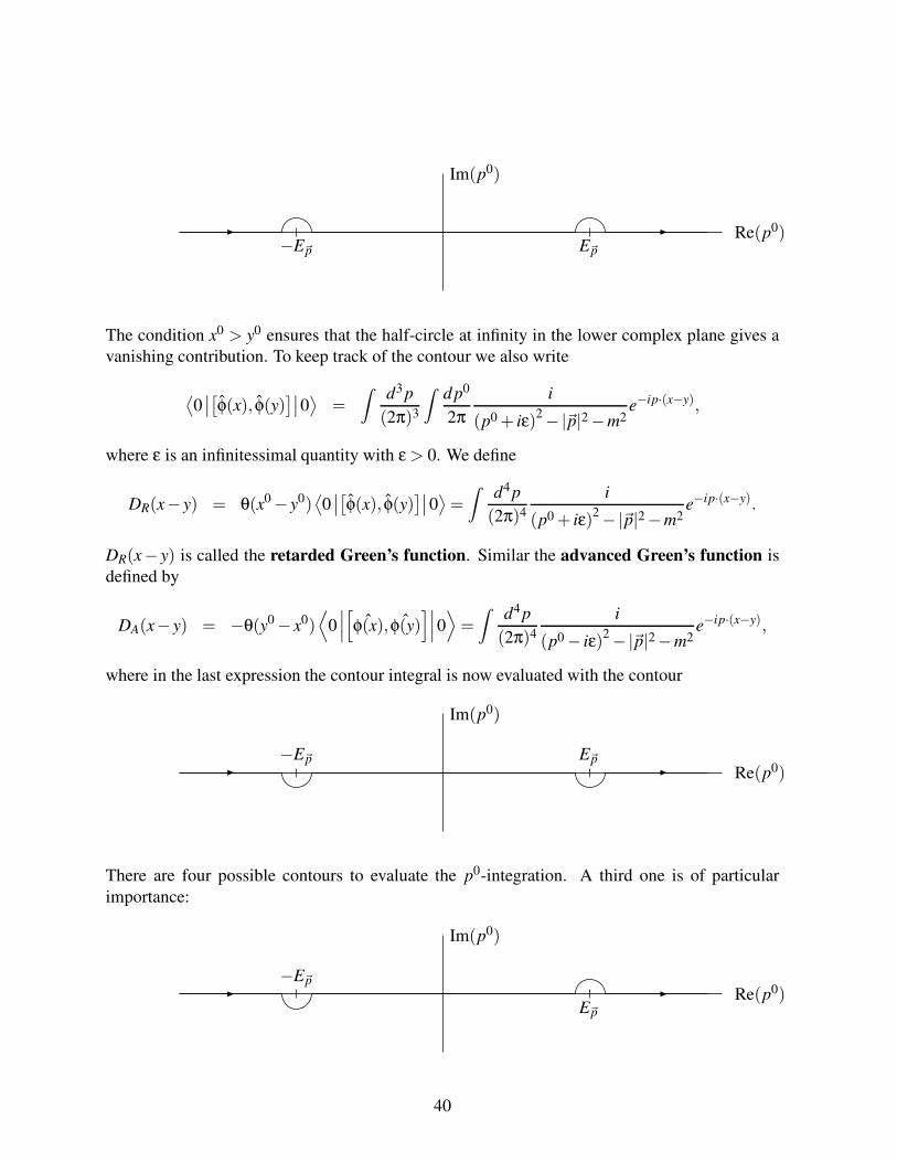
DR(x− y) is called the retarded Green’s function. Similar the advanced Green’s function is
defined by
DA(x− y) = −θ(y0− x0)⟨
0
∣∣∣
[ˆφ(x), ˆφ(y)
]∣∣∣0⟩
=
∫d4p
(2π)4
i
(p0− iε)2−|~p|2−m2
e−ip·(x−y),
where in the last expression the contour integral is now evaluated with the contour
Re(p0)
Im(p0)
−E~p E~p
There are four possible contours to evaluate the p0-integration. A third one is of particular
importance:
Re(p0)
Im(p0)
−E~p
E~p
40
This corresponds to the integral
DF(x− y) =
∫d4 p
(2π)4
i
p2−m2 + iεe−ip·(x−y),
Again, the +iε-prescription ensures that the poles are avoided as shown in the figure above.
If x0 > y0 we can close the contour below and obtain D(x− y). If x0 < y0 we close the con-
tour above and obtain D(y− x). Therefore
DF(x− y) =
D(x− y) for x0 > y0
D(y− x) for x0 < y0
= θ(x0− y0)⟨0∣∣φ(x)φ(y)
∣∣0⟩+θ(y0− x0)
⟨0∣∣φ(y)φ(x)
∣∣0⟩
=⟨0∣∣T φ(x)φ(y)
∣∣0⟩
In the last expression the time-ordering symbol T occurs, which orders operators from right to
left in non-decreasing time. Thus
T φ(x)φ(y) =
φ(x)φ(y) for x0 > y0,
φ(y)φ(x) for x0 < y0.
The quantity DF(x− y) is called the Feynman propagator. Let’s have a look at
(+m2
)DF(x− y) =
(+m2
)∫
d4p
(2π)4
i
p2−m2e−ip·(x−y)
=∫
d4p
(2π)4
i
p2−m2(−p2 +m2)e−ip·(x−y)
= −iδ4(x− y).
Therefore, if we look at the Fourier transform DF(p)
DF(x− y) =∫
d4p
(2π)4e−ip·(x−y)DF(p),
we obtain an algebraic equation for DF(p):
(p2−m2)DF(p) = i.
Summary: The Feynman propagator in momentum space is obtained from an algebraic equation.
The integration contour in the p0-plane is given by the iε-prescription. For the Klein-Gordon
propagator we have
DF(p) =i
p2−m2 + iε.
41
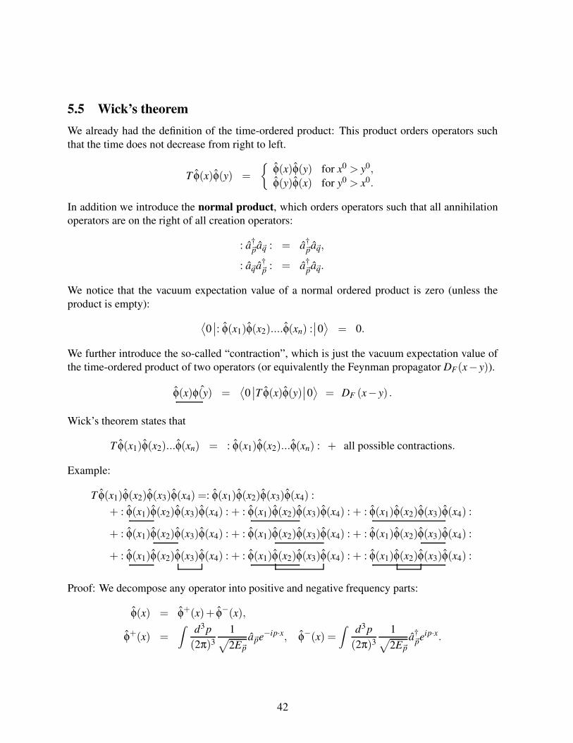
5.5 Wick’s theorem
We already had the definition of the time-ordered product: This product orders operators such
that the time does not decrease from right to left.
T φ(x)φ(y) =
φ(x)φ(y) for x0 > y0,
φ(y)φ(x) for y0 > x0.
In addition we introduce the normal product, which orders operators such that all annihilation
operators are on the right of all creation operators:
: a†~pa~q : = a
†~pa~q,
: a~qa†~p : = a
†~pa~q.
We notice that the vacuum expectation value of a normal ordered product is zero (unless the
product is empty):
⟨0∣∣: φ(x1)φ(x2)....φ(xn) :
∣∣0⟩
= 0.
We further introduce the so-called “contraction”, which is just the vacuum expectation value of
the time-ordered product of two operators (or equivalently the Feynman propagator DF(x− y)).
φ(x) ˆφ(y) =⟨0∣∣T φ(x)φ(y)
∣∣0⟩
= DF (x− y) .
Wick’s theorem states that
T φ(x1)φ(x2)...φ(xn) = : φ(x1)φ(x2)...φ(xn) : + all possible contractions.
Example:
T φ(x1)φ(x2)φ(x3)φ(x4) =: φ(x1)φ(x2)φ(x3)φ(x4) :
+ : φ(x1)φ(x2)φ(x3)φ(x4) : + : φ(x1)φ(x2)φ(x3)φ(x4) : + : φ(x1)φ(x2)φ(x3)φ(x4) :
+ : φ(x1)φ(x2)φ(x3)φ(x4) : + : φ(x1)φ(x2)φ(x3)φ(x4) : + : φ(x1)φ(x2)φ(x3)φ(x4) :
+ : φ(x1)φ(x2)φ(x3)φ(x4) : + : φ(x1)φ(x2)φ(x3)φ(x4) : + : φ(x1)φ(x2)φ(x3)φ(x4) :
Proof: We decompose any operator into positive and negative frequency parts:
φ(x) = φ+(x)+ φ−(x),
φ+(x) =∫
d3p
(2π)3
1√
2E~pa~pe−ip·x, φ−(x) =
∫d3p
(2π)3
1√
2E~pa
†~peip·x.
42
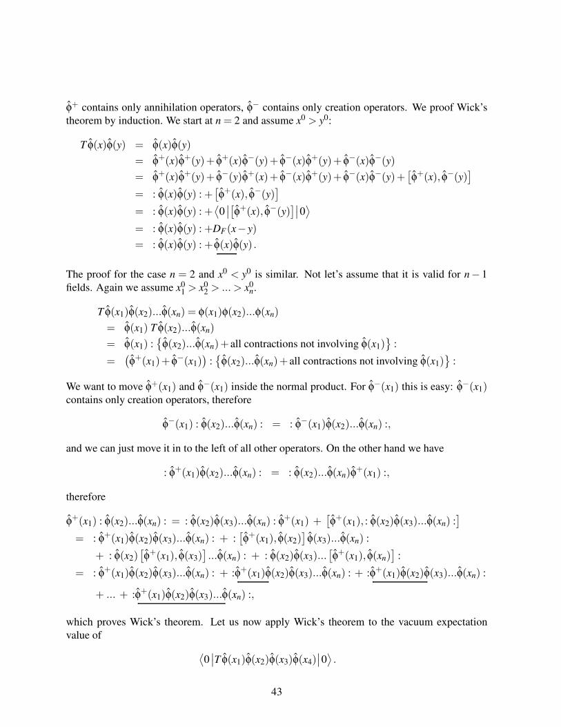
φ+ contains only annihilation operators, φ− contains only creation operators. We proof Wick’s
theorem by induction. We start at n = 2 and assume x0 > y0:
T φ(x)φ(y) = φ(x)φ(y)
= φ+(x)φ+(y)+ φ+(x)φ−(y)+ φ−(x)φ+(y)+ φ−(x)φ−(y)
= φ+(x)φ+(y)+ φ−(y)φ+(x)+ φ−(x)φ+(y)+ φ−(x)φ−(y)+[φ+(x), φ−(y)
]
= : φ(x)φ(y) : +[φ+(x), φ−(y)
]
= : φ(x)φ(y) : +⟨0∣∣[φ+(x), φ−(y)
]∣∣0⟩
= : φ(x)φ(y) : +DF(x− y)
= : φ(x)φ(y) : + φ(x)φ(y) .
The proof for the case n = 2 and x0 < y0 is similar. Not let’s assume that it is valid for n− 1
fields. Again we assume x01 > x0
2 > ... > x0n.
T φ(x1)φ(x2)...φ(xn) = φ(x1)φ(x2)...φ(xn)
= φ(x1) T φ(x2)...φ(xn)
= φ(x1) :
φ(x2)...φ(xn)+ all contractions not involving φ(x1)
:
=(φ+(x1)+ φ−(x1)
):
φ(x2)...φ(xn)+ all contractions not involving φ(x1)
:
We want to move φ+(x1) and φ−(x1) inside the normal product. For φ−(x1) this is easy: φ−(x1)contains only creation operators, therefore
φ−(x1) : φ(x2)...φ(xn) : = : φ−(x1)φ(x2)...φ(xn) :,
and we can just move it in to the left of all other operators. On the other hand we have
: φ+(x1)φ(x2)...φ(xn) : = : φ(x2)...φ(xn)φ+(x1) :,
therefore
φ+(x1) : φ(x2)...φ(xn) : = : φ(x2)φ(x3)...φ(xn) : φ+(x1) +[φ+(x1), : φ(x2)φ(x3)...φ(xn) :
]
= : φ+(x1)φ(x2)φ(x3)...φ(xn) : + :[φ+(x1), φ(x2)
]φ(x3)...φ(xn) :
+ : φ(x2)[φ+(x1), φ(x3)
]...φ(xn) : + : φ(x2)φ(x3)...
[φ+(x1), φ(xn)
]:
= : φ+(x1)φ(x2)φ(x3)...φ(xn) : + :φ+(x1)φ(x2)φ(x3)...φ(xn) : + :φ+(x1)φ(x2)φ(x3)...φ(xn) :
+ ... + :φ+(x1)φ(x2)φ(x3)...φ(xn) :,
which proves Wick’s theorem. Let us now apply Wick’s theorem to the vacuum expectation
value of
⟨0∣∣T φ(x1)φ(x2)φ(x3)φ(x4)
∣∣0⟩.
43

By construction, the vacuum expectation value of a non-empty normal product vanishes, there-
fore
⟨0∣∣T φ(x1)φ(x2)φ(x3)φ(x4)
∣∣0⟩=
=
⟨
0
∣∣∣∣∣: φ(x1)φ(x2)φ(x3)φ(x4) :
∣∣∣∣∣0
⟩
+
⟨
0
∣∣∣∣∣: φ(x1)φ(x2)φ(x3)φ(x4) :
∣∣∣∣∣0
⟩
+
⟨
0
∣∣∣∣∣: φ(x1)φ(x2)φ(x3)φ(x4) :
∣∣∣∣∣0
⟩
=⟨0∣∣T φ(x1)φ(x2)
∣∣0⟩⟨
0∣∣T φ(x3)φ(x4)
∣∣0⟩+⟨0∣∣T φ(x1)φ(x3)
∣∣0⟩⟨
0∣∣T φ(x2)φ(x4)
∣∣0⟩
+⟨0∣∣T φ(x1)φ(x4)
∣∣0⟩⟨
0∣∣T φ(x2)φ(x3)
∣∣0⟩
= DF(x1− x2)DF(x3− x4)+DF(x1− x3)DF(x2− x4)+DF(x1− x4)DF(x2− x3).
Graphically,
⟨0∣∣T φ(x1)φ(x2)φ(x3)φ(x4)
∣∣0⟩
=
1 2
34
+
1 2
34
+
1 2
34
.
5.6 Interacting fields
Up to now we considered “free” fields, e.g. fields without any interactions. For the free Klein-
Gordon field we had the Lagrange density
L0 =1
2
(∂µφ)(∂µφ)− 1
2m2φ2.
In this theory, no interactions and no scattering occurs. Let us start to look at more interesting
theories with interactions:
L =1
2
(∂µφ)(∂µφ)− 1
2m2φ2− λ
4!φ4,
where λ is a dimensionless coupling constant. This theory is often called “phi-fourth” theory and
one of the simplest theories with interactions. Obviously,
L = L0 +Lint, Lint =−λ
4!φ4.
The “classical” equation of motion for the φ4 theory is
(+m2
)φ = − λ
3!φ3,
which cannot be solved by Fourier analysis as the free Klein-Gordon equation. For λ = 0 we
recover the Klein-Gordon equation. If λ is small we may treat the interacting theory by pertur-
bation theory.
44
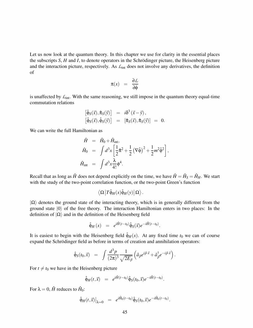
Let us now look at the quantum theory. In this chapter we use for clarity in the essential places
the subscripts S, H and I, to denote operators in the Schrödinger picture, the Heisenberg picture
and the interaction picture, respectively. As Lint does not involve any derivatives, the definition
of
π(x) =∂L
∂φ
is unaffected by Lint. With the same reasoning, we still impose in the quantum theory equal-time
commutation relations
[φS(~x), πS(~y)
]= iδ3 (~x−~y) ,
[φS(~x), φS(~y)
]= [πS(~x), πS(~y)] = 0.
We can write the full Hamiltonian as
H = H0 + Hint,
H0 =
∫d3x
[1
2π2 +
1
2
(∇φ)2
+1
2m2φ2
]
,
Hint =∫
d3xλ
4!φ4.
Recall that as long as H does not depend explicitly on the time, we have H = HS = HH . We start
with the study of the two-point correlation function, or the two-point Green’s function
⟨Ω∣∣T φH(x)φH(y)
∣∣Ω⟩.
|Ω〉 denotes the ground state of the interacting theory, which is in generally different from the
ground state |0〉 of the free theory. The interaction Hamiltonian enters in two places: In the
definition of |Ω〉 and in the definition of the Heisenberg field
φH (x) = eiH(t−t0)φS(~x)e−iH(t−t0).
It is easiest to begin with the Heisenberg field φH(x). At any fixed time t0 we can of course
expand the Schrödinger field as before in terms of creation and annihilation operators:
φS(t0,~x) =∫
d3p
(2π)3
1√
2E~p
(
a~pei~p·~x + a†~pe−i~p·~x
)
.
For t 6= t0 we have in the Heisenberg picture
φH(t,~x) = eiH(t−t0)φS(t0,~x)e−iH(t−t0).
For λ = 0, H reduces to H0:
φH(t,~x)∣∣λ=0
= eiH0(t−t0)φS(t0,~x)e−iH0(t−t0).
45
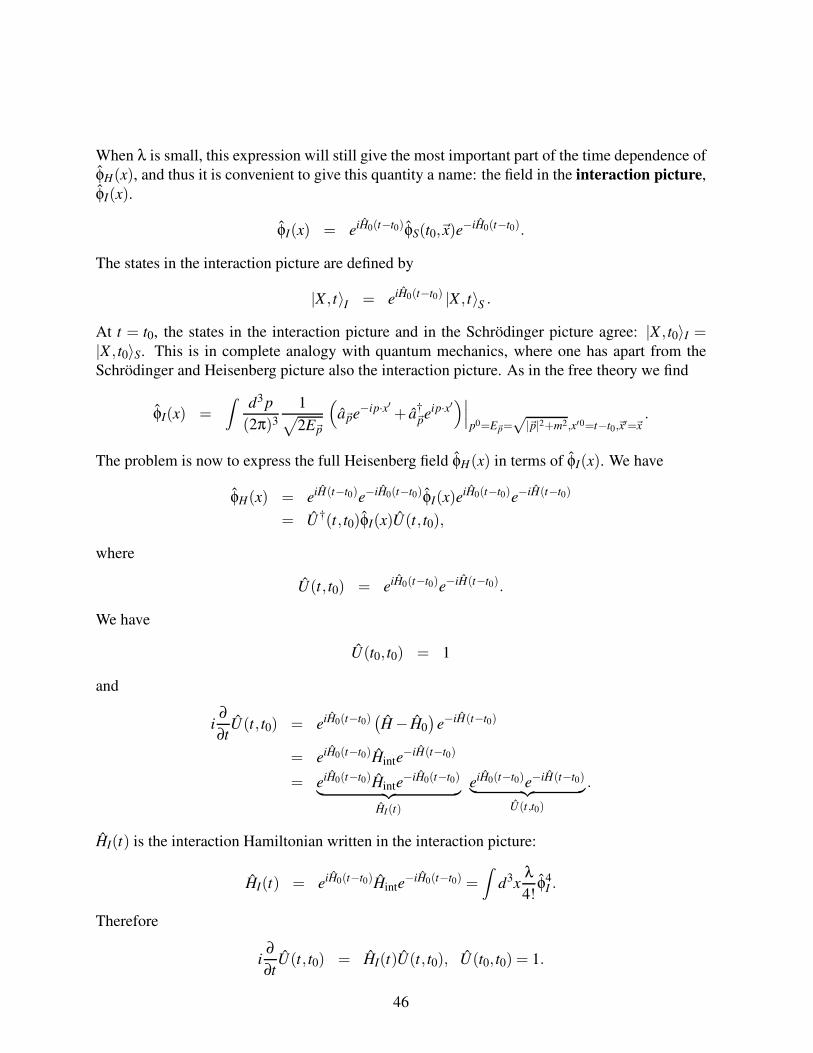
When λ is small, this expression will still give the most important part of the time dependence of
φH(x), and thus it is convenient to give this quantity a name: the field in the interaction picture,
φI(x).
φI(x) = eiH0(t−t0)φS(t0,~x)e−iH0(t−t0).
The states in the interaction picture are defined by
|X , t〉I = eiH0(t−t0) |X , t〉S .
At t = t0, the states in the interaction picture and in the Schrödinger picture agree: |X , t0〉I =|X , t0〉S. This is in complete analogy with quantum mechanics, where one has apart from the
Schrödinger and Heisenberg picture also the interaction picture. As in the free theory we find
φI(x) =
∫d3 p
(2π)3
1√
2E~p
(
a~pe−ip·x′+ a†~peip·x′
)∣∣∣
p0=E~p=√|~p|2+m2,x′0=t−t0,~x′=~x
.
The problem is now to express the full Heisenberg field φH(x) in terms of φI(x). We have
φH(x) = eiH(t−t0)e−iH0(t−t0)φI(x)eiH0(t−t0)e−iH(t−t0)
= U†(t, t0)φI(x)U(t, t0),
where
U(t, t0) = eiH0(t−t0)e−iH(t−t0).
We have
U(t0, t0) = 1
and
i∂
∂tU(t, t0) = eiH0(t−t0)
(H− H0
)e−iH(t−t0)
= eiH0(t−t0)Hinte−iH(t−t0)
= eiH0(t−t0)Hinte−iH0(t−t0)
︸ ︷︷ ︸
HI(t)
eiH0(t−t0)e−iH(t−t0)︸ ︷︷ ︸
U(t,t0)
.
HI(t) is the interaction Hamiltonian written in the interaction picture:
HI(t) = eiH0(t−t0)Hinte−iH0(t−t0) =
∫d3x
λ
4!φ4
I .
Therefore
i∂
∂tU(t, t0) = HI(t)U(t, t0), U(t0, t0) = 1.
46
A solution is given by
U(t, t0) = 1+(−i)
t∫
t0
dt1 HI(t1)+(−i)2
t∫
t0
dt1
t1∫
t0
dt2 HI(t1)HI(t2)
+(−i)3
t∫
t0
dt1
t1∫
t0
dt2
t2∫
t0
dt3 HI(t1)HI(t2)HI(t3)+ ...
This solution can be verified by differentiation. The initial condition U(t0, t0) = 1 is obviously
satisfied. Note that the various factors of HI stand in time order, later on the left. Note that
t∫
t0
dt1
t1∫
t0
dt2 HI(t1)HI(t2) =1
2
t∫
t0
dt1
t∫
t0
dt2 T(HI(t1)HI(t2)
).
Similar
t∫
t0
dt1
t1∫
t0
dt2...
tn−1∫
t0
dtn HI(t1)HI(t2)...HI(tn) =1
n!
t∫
t0
dt1
t∫
t0
dt2...
t∫
t0
dtn T(HI(t1)HI(t2)...HI(tn)
).
Therefore
U(t, t0) = 1+(−i)
t∫
t0
dt1 HI(t1)+(−i)2
2!
t∫
t0
dt1
t∫
t0
dt2 T(HI(t1)HI(t2)
)
+(−i)3
3!
t∫
t0
dt1
t∫
t0
dt2
t∫
t0
dt3 T(HI(t1)HI(t2)HI(t3)
)+ ...
= T
exp
−i
t∫
t0
dt ′ HI(t′)
.
Therefore we have expressed the full field φH in terms of φI;
φH(x) = U†(t, t0)φI(x)U(t, t0),
We can generalise the evolution operator to take as the second argument values other than our
reference time t0:
U(t, t ′) = T
exp
−i
t∫
t ′
dt ′′ HI(t′′)
.
47
U(t, t ′) satisfies
i∂
∂tU(t, t ′) = HI(t)U(t, t ′), U(t, t) = 1,
and the identities
U(t1, t2)U(t2, t3) = U(t1, t3),
U(t1, t3)U†(t2, t3) = U(t1, t2).
U(t, t ′) is unitary:
U(t, t ′)U†(t, t ′) = U(t, t) = 1.
We further have
U(t, t ′) = U(t, t0)U†(t ′, t0)
= eiH0(t−t0)e−iH(t−t ′)e−iH0(t′−t0),
In particular we have
U(t0,−T ) = e−iH(t0−(−T ))e−iH0((−T )−t0).
Let us now discuss the ground state |Ω〉. Imagine starting with |0〉, the ground state of H0 and
evolving through time with H:
e−iHT |0〉 = ∑n
e−iEfulln T |nfull〉〈nfull|0〉.
Here we inserted a complete set of states. Efulln and |nfull〉 are the eigenvalues and eigenstates of
the full Hamiltonian H. The eigenvalues and eigenstates of the free Hamiltonian will be denoted
by En and |n〉. We define the zero of the energy by
H0|0〉 = 0.
We single out the ground state |Ω〉= |0full〉:
e−iHT |0〉 = e−iEfull0 T |Ω〉〈Ω|0〉+ ∑
n6=0
e−iEfulln T |nfull〉〈nfull|0〉,
where Efull0 = 〈Ω|H|Ω〉. Since Efull
n > Efull0 for n > 0 the additional terms disappear, if we send
T → ∞(1− iε). Therefore
|Ω〉 = limT→∞(1−iε)
(
e−iEfull0 T 〈Ω|0〉
)−1
e−iHT |0〉.
48
Since T is now very large, we can shift it by a small constant:
|Ω〉 = limT→∞(1−iε)
(
e−iEfull0 (T+t0)〈Ω|0〉
)−1
e−iH(T+t0)|0〉
= limT→∞(1−iε)
(
e−iEfull0 (t0−(−T ))〈Ω|0〉
)−1
e−iH(t0−(−T ))e−iH0((−T )−t0)|0〉
= limT→∞(1−iε)
(
e−iEfull0 (t0−(−T ))〈Ω|0〉
)−1
U(t0,−T )|0〉
In the second line we have used H0|0〉= 0. Similar, we can express 〈Ω| as
〈Ω| = limT→∞(1−iε)
〈0|U(T, t0)(
e−iEfull0 (T−t0)〈0|Ω〉
)−1
.
Therefore we have for x0 > y0 > t0 (we drop the subscript H for φ(x) = φH(x)):⟨Ω∣∣T φ(x)φ(y)
∣∣Ω⟩=
= limT→∞(1−iε)
〈0|U(T, t0)U†(x0, t0)φI(x)U(x0, t0)U
†(y0, t0)φI(x)U(y0, t0)U(t0,−T )|0〉e−2iEfull
0 T 〈Ω|0〉〈0|Ω〉
= limT→∞(1−iε)
〈0|U(T,x0)φI(x)U(x0,y0)φI(x)U(y0,−T )|0〉e−2iEfull
0 T |〈0|Ω〉|2Now
1 = 〈Ω|Ω〉= 〈0|U(T, t0)U(t0,−T )|0〉e−2iEfull
0 T |〈0|Ω〉|2=〈0|U(T,−T )|0〉
e−2iEfull0 T |〈0|Ω〉|2
.
Therefore we have for x0 > y0
⟨Ω∣∣T φ(x)φ(y)
∣∣Ω⟩
= limT→∞(1−iε)
〈0|U(T,x0)φI(x)U(x0,y0)φI(x)U(y0,−T )|0〉〈0|U(T,−T )|0〉
.
We notice that all fields are in time-order. The final formula, valid for any x0 and y0 reads
⟨Ω∣∣T φ(x)φ(y)
∣∣Ω⟩
= limT→∞(1−iε)
⟨0∣∣T
φI(x)φI(y)U(T,−T )∣∣0⟩
⟨0∣∣U(T,−T )
∣∣0⟩
= limT→∞(1−iε)
⟨
0
∣∣∣∣T
φI(x)φI(y)exp
[
−iT∫−T
dt HI(t)
]∣∣∣∣0
⟩
⟨
0
∣∣∣∣T
exp
[
−iT∫−T
dt HI(t)
]∣∣∣∣0
⟩ .
There is an obvious generalisation to more than two fields:⟨Ω∣∣T φ(x1)φ(x2)...φ(xn)
∣∣Ω⟩=
= limT→∞(1−iε)
⟨
0
∣∣∣∣T
φI(x1)φI(x2)...φI(xn)exp
[
−iT∫−T
dt HI(t)
]∣∣∣∣0
⟩
⟨
0
∣∣∣∣T
exp
[
−iT∫−T
dt HI(t)
]∣∣∣∣0
⟩ .
49
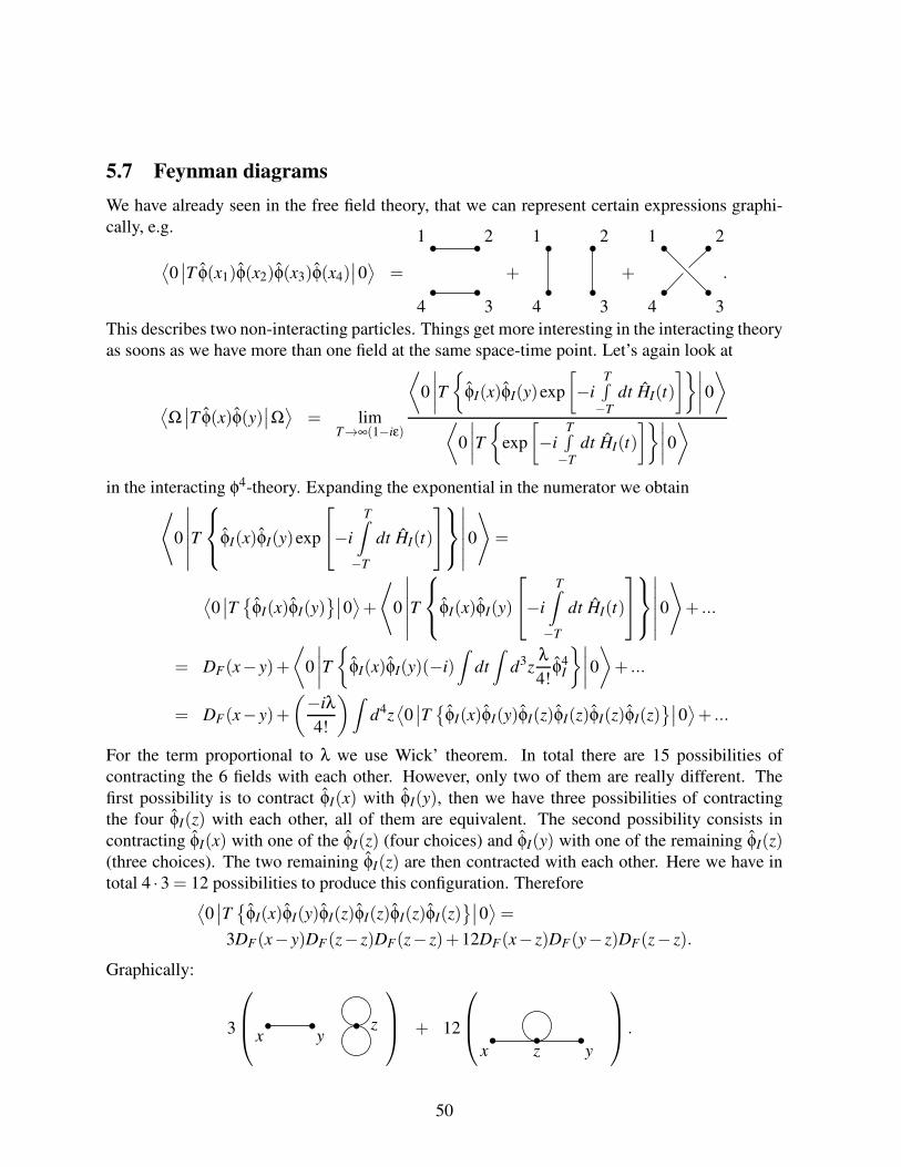
5.7 Feynman diagrams
We have already seen in the free field theory, that we can represent certain expressions graphi-
cally, e.g.
⟨0∣∣T φ(x1)φ(x2)φ(x3)φ(x4)
∣∣0⟩
=
1 2
34
+
1 2
34
+
1 2
34
.
This describes two non-interacting particles. Things get more interesting in the interacting theory
as soons as we have more than one field at the same space-time point. Let’s again look at
⟨Ω∣∣T φ(x)φ(y)
∣∣Ω⟩
= limT→∞(1−iε)
⟨
0
∣∣∣∣T
φI(x)φI(y)exp
[
−iT∫−T
dt HI(t)
]∣∣∣∣0
⟩
⟨
0
∣∣∣∣T
exp
[
−iT∫−T
dt HI(t)
]∣∣∣∣0
⟩
in the interacting φ4-theory. Expanding the exponential in the numerator we obtain
⟨
0
∣∣∣∣∣∣
T
φI(x)φI(y)exp
−i
T∫
−T
dt HI(t)
∣∣∣∣∣∣
0
⟩
=
⟨0∣∣T
φI(x)φI(y)∣∣0⟩+
⟨
0
∣∣∣∣∣∣
T
φI(x)φI(y)
−i
T∫
−T
dt HI(t)
∣∣∣∣∣∣
0
⟩
+ ...
= DF(x− y)+
⟨
0
∣∣∣∣T
φI(x)φI(y)(−i)∫
dt
∫d3z
λ
4!φ4
I
∣∣∣∣0
⟩
+ ...
= DF(x− y)+
(−iλ
4!
)∫d4z⟨0∣∣T
φI(x)φI(y)φI(z)φI(z)φI(z)φI(z)∣∣0⟩+ ...
For the term proportional to λ we use Wick’ theorem. In total there are 15 possibilities of
contracting the 6 fields with each other. However, only two of them are really different. The
first possibility is to contract φI(x) with φI(y), then we have three possibilities of contracting
the four φI(z) with each other, all of them are equivalent. The second possibility consists in
contracting φI(x) with one of the φI(z) (four choices) and φI(y) with one of the remaining φI(z)(three choices). The two remaining φI(z) are then contracted with each other. Here we have in
total 4 ·3 = 12 possibilities to produce this configuration. Therefore⟨0∣∣T
φI(x)φI(y)φI(z)φI(z)φI(z)φI(z)∣∣0⟩=
3DF(x− y)DF(z− z)DF(z− z)+12DF(x− z)DF(y− z)DF(z− z).
Graphically:
3
x y
z
+ 12
x z y
.
50
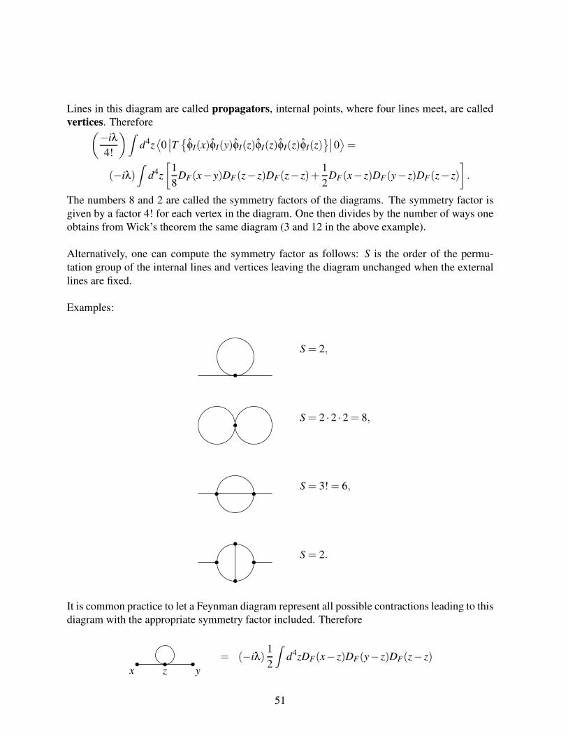
Lines in this diagram are called propagators, internal points, where four lines meet, are called
vertices. Therefore(−iλ
4!
)∫d4z⟨0∣∣T
φI(x)φI(y)φI(z)φI(z)φI(z)φI(z)∣∣0⟩=
(−iλ)
∫d4z
[1
8DF(x− y)DF(z− z)DF(z− z)+
1
2DF(x− z)DF(y− z)DF(z− z)
]
.
The numbers 8 and 2 are called the symmetry factors of the diagrams. The symmetry factor is
given by a factor 4! for each vertex in the diagram. One then divides by the number of ways one
obtains from Wick’s theorem the same diagram (3 and 12 in the above example).
Alternatively, one can compute the symmetry factor as follows: S is the order of the permu-
tation group of the internal lines and vertices leaving the diagram unchanged when the external
lines are fixed.
Examples:
S = 2,
S = 2 ·2 ·2 = 8,
S = 3! = 6,
S = 2.
It is common practice to let a Feynman diagram represent all possible contractions leading to this
diagram with the appropriate symmetry factor included. Therefore
x z y
= (−iλ)1
2
∫d4zDF(x− z)DF(y− z)DF(z− z)
51
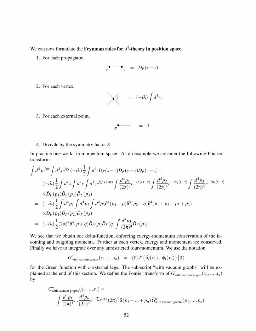
We can now formulate the Feynman rules for φ4-theory in position space:
1. For each propagator,
x y = DF(x− y).
2. For each vertex,
z = (−iλ)∫
d4z.
3. For each external point,
x = 1.
4. Divivde by the symmetry factor S.
In practice one works in momentum space. As an example we consider the following Fourier
transform∫d4xeipx
∫d4yeiqy (−iλ)
1
2
∫d4zDF(x− z)DF(y− z)DF(z− z) =
(−iλ)1
2
∫d4x
∫d4y
∫d4zei(px+qy)
∫d4p1
(2π)4e−ip1(x−z)
∫d4 p2
(2π)4e−ip2(y−z)
∫d4 p3
(2π)4e−ip3(z−z)
×DF(p1)DF(p2)DF(p3)
= (−iλ)1
2
∫d4 p1
∫d4p2
∫d4 p3δ4(p1− p)δ4(p2−q)δ4(p1 + p2− p3 + p3)
×DF(p1)DF(p2)DF(p3)
= (−iλ)1
2(2π)4δ4(p+q)DF(p)DF(q)
∫d4p3
(2π)4DF(p3)
We see that we obtain one delta-function, enforcing energy-momentum conservation of the in-
coming and outgoing momenta. Further at each vertex, energy and momentum are conserved.
Finally we have to integrate over any unrestricted four-momentum. We use the notation
Gnwith vacuum graphs(x1, ...,xn) =
⟨0∣∣T
φI(x1)...φI(xn)∣∣0⟩
for the Green function with n external legs. The sub-script “with vacuum graphs” will be ex-
plained at the end of this section. We define the Fourier transform of Gnwith vacuum graphs(x1, ...,xn)
by
Gnwith vacuum graphs(x1, ...,xn) =∫
d4p1
(2π)4...
d4pn
(2π)4e−i∑ p jx j (2π)4 δ(p1 + ...+ pn) Gn
with vacuum graphs(p1, ..., pn)
52
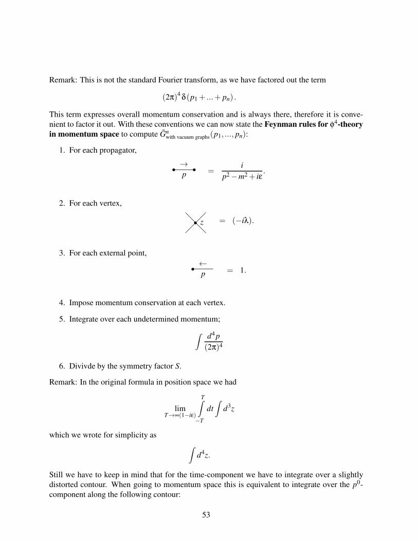
Remark: This is not the standard Fourier transform, as we have factored out the term
(2π)4 δ(p1 + ...+ pn) .
This term expresses overall momentum conservation and is always there, therefore it is conve-
nient to factor it out. With these conventions we can now state the Feynman rules for φ4-theory
in momentum space to compute Gnwith vacuum graphs(p1, ..., pn):
1. For each propagator,
p
→=
i
p2−m2 + iε.
2. For each vertex,
z = (−iλ).
3. For each external point,
p
←= 1.
4. Impose momentum conservation at each vertex.
5. Integrate over each undetermined momentum;
∫d4 p
(2π)4
6. Divivde by the symmetry factor S.
Remark: In the original formula in position space we had
limT→∞(1−iε)
T∫
−T
dt
∫d3z
which we wrote for simplicity as
∫d4z.
Still we have to keep in mind that for the time-component we have to integrate over a slightly
distorted contour. When going to momentum space this is equivalent to integrate over the p0-
component along the following contour:
53
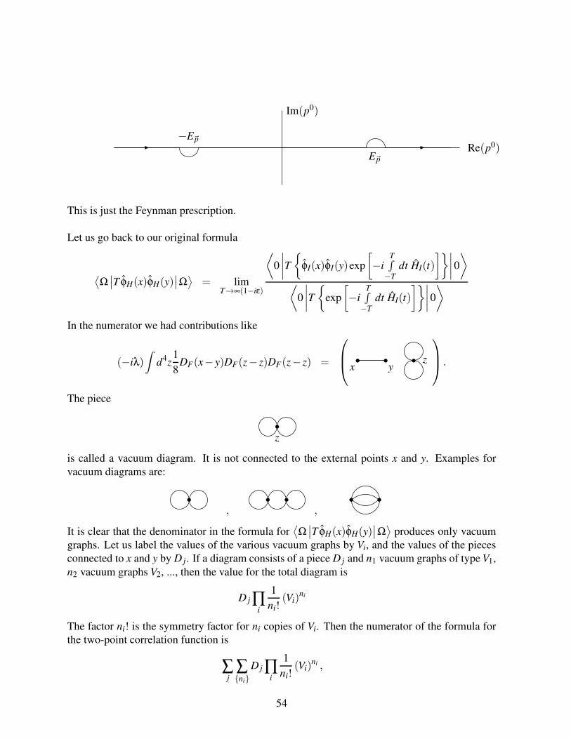
Re(p0)
Im(p0)
−E~p
E~p
This is just the Feynman prescription.
Let us go back to our original formula
⟨Ω∣∣T φH(x)φH(y)
∣∣Ω⟩
= limT→∞(1−iε)
⟨
0
∣∣∣∣T
φI(x)φI(y)exp
[
−iT∫−T
dt HI(t)
]∣∣∣∣0
⟩
⟨
0
∣∣∣∣T
exp
[
−iT∫−T
dt HI(t)
]∣∣∣∣0
⟩
In the numerator we had contributions like
(−iλ)
∫d4z
1
8DF(x− y)DF(z− z)DF(z− z) =
x y
z
.
The piece
z
is called a vacuum diagram. It is not connected to the external points x and y. Examples for
vacuum diagrams are:
, ,
It is clear that the denominator in the formula for⟨Ω∣∣T φH(x)φH(y)
∣∣Ω⟩
produces only vacuum
graphs. Let us label the values of the various vacuum graphs by Vi, and the values of the pieces
connected to x and y by D j. If a diagram consists of a piece D j and n1 vacuum graphs of type V1,
n2 vacuum graphs V2, ..., then the value for the total diagram is
D j ∏i
1
ni!(Vi)
ni
The factor ni! is the symmetry factor for ni copies of Vi. Then the numerator of the formula for
the two-point correlation function is
∑j
∑ni
D j ∏i
1
ni!(Vi)
ni ,
54
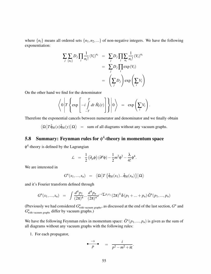
where ni means all ordered sets n1,n2, ... of non-negative integers. We have the following
exponentiation:
∑j
∑ni
D j ∏i
1
ni!(Vi)
ni = ∑j
D j ∏i
∑ni
1
ni!(Vi)
ni
= ∑j
D j ∏i
exp(Vi)
=
(
∑j
D j
)
exp
(
∑i
Vi
)
On the other hand we find for the denominator
⟨
0
∣∣∣∣∣∣
T
exp
−i
T∫
−T
dt HI(t)
∣∣∣∣∣∣
0
⟩
= exp
(
∑i
Vi
)
.
Therefore the exponential cancels between numerator and denominator and we finally obtain
⟨Ω∣∣T φH(x)φH(y)
∣∣Ω⟩
= sum of all diagrams without any vacuum graphs.
5.8 Summary: Feynman rules for φ4-theory in momentum space
φ4-theory is defined by the Lagrangian
L =1
2
(∂µφ)(∂µφ)− 1
2m2φ2− λ
4!φ4.
We are interested in
Gn(x1, ...,xn) =⟨Ω∣∣T
φH(x1)...φH(xn)∣∣Ω⟩
and it’s Fourier transform defined through
Gn(x1, ...,xn) =∫
d4p1
(2π)4...
d4pn
(2π)4e−i∑ p jx j (2π)4 δ(p1 + ...+ pn) Gn(p1, ..., pn)
(Previously we had considered Gnwith vacuum graphs, as discussed at the end of the last section, Gn and
Gnwith vacuum graphs differ by vacuum graphs.)
We have the following Feynman rules in momentum space: Gn(p1, ..., pn) is given as the sum of
all diagrams without any vacuum graphs with the following rules:
1. For each propagator,
p
→=
i
p2−m2 + iε.
55
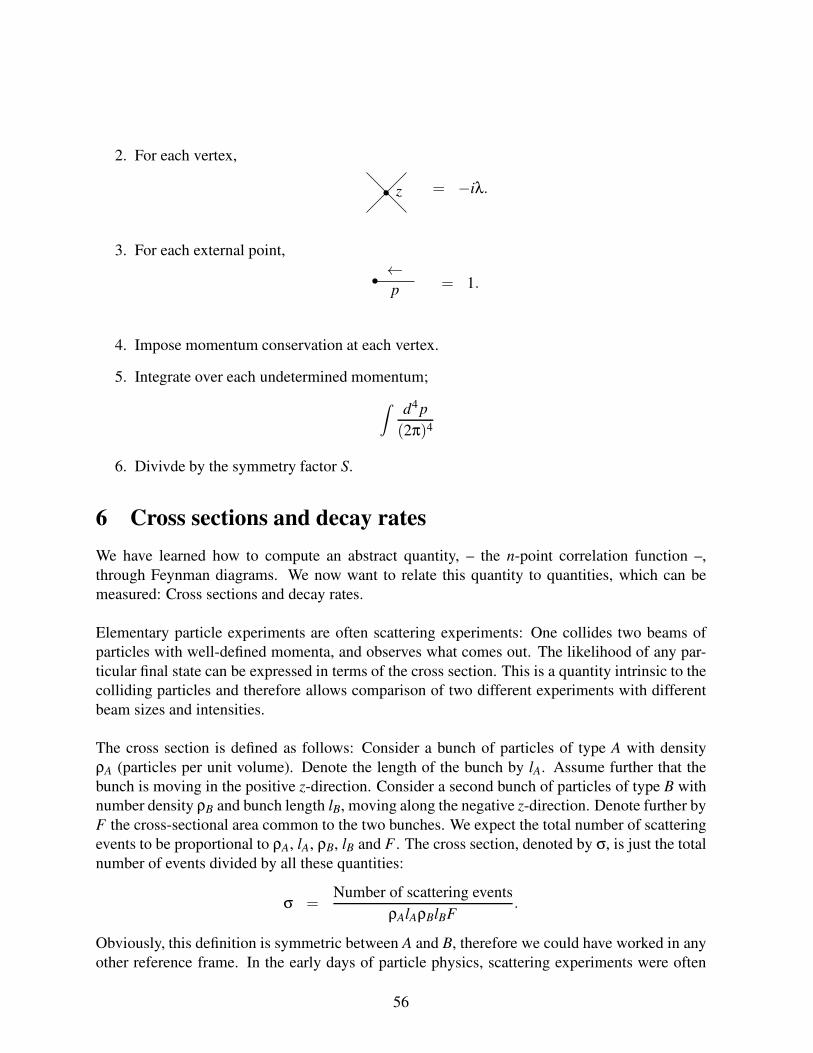
2. For each vertex,
z = −iλ.
3. For each external point,
p
←= 1.
4. Impose momentum conservation at each vertex.
5. Integrate over each undetermined momentum;
∫d4 p
(2π)4
6. Divivde by the symmetry factor S.
6 Cross sections and decay rates
We have learned how to compute an abstract quantity, – the n-point correlation function –,
through Feynman diagrams. We now want to relate this quantity to quantities, which can be
measured: Cross sections and decay rates.
Elementary particle experiments are often scattering experiments: One collides two beams of
particles with well-defined momenta, and observes what comes out. The likelihood of any par-
ticular final state can be expressed in terms of the cross section. This is a quantity intrinsic to the
colliding particles and therefore allows comparison of two different experiments with different
beam sizes and intensities.
The cross section is defined as follows: Consider a bunch of particles of type A with density
ρA (particles per unit volume). Denote the length of the bunch by lA. Assume further that the
bunch is moving in the positive z-direction. Consider a second bunch of particles of type B with
number density ρB and bunch length lB, moving along the negative z-direction. Denote further by
F the cross-sectional area common to the two bunches. We expect the total number of scattering
events to be proportional to ρA, lA, ρB, lB and F . The cross section, denoted by σ, is just the total
number of events divided by all these quantities:
σ =Number of scattering events
ρAlAρBlBF.
Obviously, this definition is symmetric between A and B, therefore we could have worked in any
other reference frame. In the early days of particle physics, scattering experiments were often
56
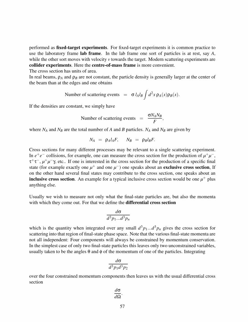
performed as fixed-target experiments. For fixed-target experiments it is common practice to
use the laboratory frame lab frame. In the lab frame one sort of particles is at rest, say A,
while the other sort moves with velocity v towards the target. Modern scattering experiments are
collider experiments. Here the centre-of-mass frame is more convenient.
The cross section has units of area.
In real beams, ρA and ρB are not constant, the particle density is generally larger at the center of
the beam than at the edges and one obtains
Number of scattering events = σ lAlB
∫d2x ρA(x)ρB(x).
If the densities are constant, we simply have
Number of scattering events =σNANB
F,
where NA and NB are the total number of A and B particles. NA and NB are given by
NA = ρAlAF, NB = ρBlBF.
Cross sections for many different processes may be relevant to a single scattering experiment.
In e+e− collisions, for example, one can measure the cross section for the production of µ+µ−,
τ+τ−, µ+µ−γ, etc.. If one is interested in the cross section for the production of a specific final
state (for example exactly one µ+ and one µ−) one speaks about an exclusive cross section, If
on the other hand several final states may contribute to the cross section, one speaks about an
inclusive cross section. An example for a typical inclusive cross section would be one µ+ plus
anything else.
Usually we wish to measure not only what the final-state particles are, but also the momenta
with which they come out. For that we define the differential cross section
dσ
d3p1...d3pn
which is the quantity when integrated over any small d3p1...d3pn gives the cross section for
scattering into that region of final-state phase space. Note that the various final-state momenta are
not all independent: Four components will always be constrained by momentum conservation.
In the simplest case of only two final-state particles this leaves only two unconstrained variables,
usually taken to be the angles θ and φ of the momentum of one of the particles. Integrating
dσ
d3 p1d3 p2
over the four constrained momentum components then leaves us with the usual differential cross
section
dσ
dΩ.
57
A second measurable quantity is the decay rate of an unstable particle. The decay rate Γ of an
unstable particle A, which is assumed to be at rest, is defined as follows:
Γ =Number of decays per unit time
Number of A particles present.
The lifetime τ is the reciprocal of the sum of the decay widths into all possible final states. The
particle’s half-life time is τ · ln2.
In non-relativistic quantum mechanics, an unstable atomic state shows up in scattering exper-
iments as a resonance. Near the resonance energy E0, the scattering amplitude is given by the
Breit-Wigner-formula
f (E) ∼ 1
E−E0 + iΓ/2
The cross section therefore has a peak of the form
σ ∼ 1
(E−E0)2 +Γ2/4
The width of the resonance peak is equal to the decay rate of the unstable state. The Breit-Wigner
formula also applies to relativistic quantum mechanics. In an amplitude involving an unstable
particle of momentum p and mass m we have
1
p2−m2 + imΓ≈ 1
2E~p
(p0−E~p + i
(m/E~p
)Γ/2
) .
Remark: A correct treatment of unstable particles in higher orders in perturbation theory is a
topic of current interest.
6.1 The S-matrix
To calculate the cross section we set up wavepackets representing the initial-state particles,
evolve this initial state for a very long time with the time-evolution operator exp(−iHt) of the
full interacting field theory and overlap the resulting final state with wavepackets representing
some desired set of final-state particles.
A wavepacket is given by
|φ〉 =∫
d3k
(2π)3
1√
2E~kφ(~k)
∣∣∣~k⟩
,
where |~k〉 is a one-particle state of momentum~k in the full interacting theory and the weight
function φ(~k) is peaked around ~p.
58
We recall that we chose as normalisation for the one-particle states
〈~p|~q〉 = 2E~p(2π)3δ3 (~p−~q) .
If we further require that
∫d3k
(2π)3
∣∣∣φ(
~k)∣∣∣
2
= 1,
then we have
〈φ|φ〉 = 1.
In a typical scattering experiment one scatters two initial-state particles and one observes, say,
n final-state particles. This leads us to the definition of in- and out-states. The in-state |φAφB〉consists of the two particles A and B in the initial state, the out-state |φ1φ2...φn〉 of the n parti-
cles in the final state. In the far past (t →−∞), the in-state is described by two wave-packets,
corresponding to two well-sepatated single particle states and we may describe the in-state in
the far past as a free state. As time proceeds, the two particles start to interact and scatter. The
situation for the out-state is analogous: In the far future (t → ∞), the out-state is described by
n wave-packets, corresponding to n well-sepatated single particle states and we may describe in
the far future the out-state as a free state. States which are described in the far past or far future
as free states are called asymptotic states. We will denote a state, which corresponds at t→−∞to a free n-particle state as an in-state
|φ1φ2...φn〉in = |φ1φ2...φn; t0 =−∞〉Hand a state, which corresponds at t→ ∞ to a free n-particle state as an out-state
|φ1φ2...φn〉out = |φ1φ2...φn; t0 = ∞〉H .
The notation on the right-hand-side indicates that the Heisenberg state |φ1φ2...φn; t0〉H coincides
at t0 ∈ ±∞ with a free n-particle state. The probability we wish to compute is
P = |out 〈φ1φ2...φn |φAφB 〉in|2
The in-state |φAφB〉in has a nice interpretation as two localised wavepackets in the far past, but
due to the evolution with the full interacting Hamiltonian in e−iHt , the wave packets will in
general not stay intact as time proceeds. In a similar way, the out-state out〈φ1φ2...φn| has a nice
interpretation as n localised wavepackets in the far future, however evolving this state backwards
in time with the full interacting Hamiltonian will in general not leave the wavepackets intact.
What is important is that the in- and out-states may have a non-zero overlap, which we wish to
compute.
Let us first consider the in-states: Consider particle A at rest and particle B along the z-axis.
It is important to take the transverse displacement into account. If the wave packet of particle B
59
is not centered at x = y = 0 in the transverse plane, but at~b, this yields a factor exp(−i~b ·~kB). |~b|is called the impact parameter.
|φAφB〉in =∫
d3kA
(2π)3
∫d3kB
(2π)3
φA(~kA)φB(~kB)√
(2E~kA)(2E~kB
)e−i~b·~kB
∣∣∣~kA
~kB
⟩
in.
The wave packet of particle A is centered around pA in momentum space, the one of particle B is
centered around pB. In a similar way we could write for the out-states
out 〈φ1φ2...φn| =
(
∏f
∫d3q f
(2π)3
φ f (~q f )√
2E~q f
)
out 〈~q1~q2...~qn| .
Again, the wave packet for particle f is centered around p f in momentum space. However, in or-
der to avoid some technical difficulties it is simpler to work for the out-state not with wavepackets
but to use a state with definite momenta
out 〈~p1~p2...~pn|
and to put in various normalisation factors (essentially a factor 1/(2E~p f) for every final-state
particle) by hand.
Let us recall the connection with the Schrödinger picture:
|φ〉H = eiHt |φ, t〉S .
If we would like to indicate that a state has specific properties at a particular time t0 (e.g. for the
case at hand, if a state corresponds at t = t0 to a n-particle state with momenta ~p1, ~p2, ..., ~pn) we
will put an extra argument and write
|φ; t0〉H = eiHt |φ, t; t0〉S .
We have
out〈~p1~p2...~pn|~kA~kB〉in = lim
T→∞H〈~p1~p2...~pn;T |~kA
~kB;−T 〉H
= limT→∞ S
⟨
~p1~p2...~pn,T ;T
∣∣∣e−iH(2T )
∣∣∣~kA
~kB,−T ;−T⟩
S
The state |~p1~p2...~pn, t0; t0〉S corresponds at t = t0 to a n-particle state with momenta ~p1, ~p2, ...,
~pn and we will simply write |~p1~p2...~pn〉. Thus
out〈~p1~p2...~pn|~kA~kB〉in = lim
T→∞
⟨
~p1~p2...~pn
∣∣∣e−iH(2T )
∣∣∣~kA
~kB
⟩
.
We define the S-matrix by
out〈~p1~p2...~pn|~kA~kB〉in =
⟨
~p1~p2...~pn
∣∣S∣∣~kA
~kB
⟩
.
60
If the particles do not interact at all, S is the identity operator. Even if the theory contains
interactions, the particles have some probability of missing each other. To isolate the interesting
part of the S-matrix – that is, the part due to interactions – we define the T -matrix by
S = 1+ i(2π)4δ4
(
kA + kB−∑f
p f
)
T .
Of special interest are the matrix elements of T :
iA (kAkB→ p1 p2...pn) = 〈~p1~p2...~pn|iT |~kA~kB〉
The probability we want to compute is now
P =
(
∏f
∫d3p f
(2π)3
1
2E~p f
)
|out〈~p1~p2...~pn|φAφB〉in|2 .
The bracket in front gives the correct normalisation factor for the out-state. The in-state still
depends on the impact parameter ~b. To obtain the cross section we have to integrate over all
impact parameters:
σ =
∫d2b P(~b).
Therefore
dσd3 p1
(2π)3
d3 p2
(2π)3 ...=
(
∏f
1
2E~p f
)∫d2b
∏i=A,B
∫d3ki
(2π)3
φi(~ki)√
2E~ki
∫d3k′i(2π)3
φ∗i (~k′i)
√
2E~k′i
e−i~b·(~kB−~k′B)out〈~p1~p2...~pn|kAkB〉in out〈~p1~p2...~pn|k′Ak′B〉∗in.If we are not interested in the trivial case where no scattering case takes place, we can drop the
identity from the S-matrix and write
out〈~p1~p2...~pn|kAkB〉in = (2π)4δ4(kA + kB−∑f
p f )iA (kAkB→ p1 p2...pn) ,
out〈~p1~p2...~pn|k′Ak′B〉in = (2π)4δ4(k′A + k′B−∑f
p f )iA(k′Ak′B→ p1 p2...pn
).
We can use the second of these delta functions, together with the δ2(k⊥B − k⊥B′) to perform all six
k′ integrals. We have∫
d3k′A(2π)3
∫d3k′B(2π)3
(2π)2δ2(k⊥B − k⊥B′)(2π)4δ4(k′A + k′B− kA− kB) =
=
∫dkz
A′∫
dkzB′δ(E ′A +E ′B−EA−EB)δ(k
zA′+ kz
B′− kz
A− kzB)
=∫
dkzA′ δ(E ′A +E ′B−EA−EB)
∣∣kz
B′=kz
A+kzB−kz
A′
=1
∣∣∣
∂EA
∂kzA− ∂EB
∂kzB
∣∣∣
=1
|vA− vB|.
61
The difference |vA− vB| is the relative velocity of the beams in the lab frame. The initial wave
packets are localised in momentum space, centered around pA and pB. We evaluate all factors,
which are smooth functions of kA and kB at pA and pB. We obtain
dσd3 p1
(2π)3
d3 p2
(2π)3 ...=
(
∏f
1
2E~p f
)
|A (pA pB→ p1p2...pn)|22EA2EB |vA− vB|
∫d3kA
(2π)3
∫d3kB
(2π)3
∣∣∣φA(~kA)
∣∣∣
2 ∣∣∣φB(~kB)
∣∣∣
2
(2π)4δ4(kA + kB−∑f
p f ).
We can simplify this formula further by noting that real detectors cannot resolve small variations
of the incoming and outcoming momenta. Therefore we can approximate δ(kA + kB−∑ p f ) by
δ(pA + pB−∑ p f ) and we obtain
dσd3 p1
(2π)3
d3 p2
(2π)3 ...=
(
∏f
1
2E~p f
)
|A (pA pB→ p1 p2...pn)|22EA2EB |vA− vB|
(2π)4δ4(pA + pB−∑f
p f ).
Note that all dependence on the shape of the wave packets has disappeared.
By a similar reasoning we find for the decay rate
dΓd3 p1
(2π)3
d3 p2
(2π)3 ...=
(
∏f
1
2E~p f
)
|A (pA→ p1 p2...pn)|22mA
(2π)4δ4(pA−∑ p f ).
To obtain the total cross section or the total decay rate we integrate over all final states. If the
final state contains n identical particles, we have to be careful not to count the same final state
more then once. One possibility is to impose a strict ordering on the energies of the final state
particles
E1 > E2 > ... > En,
a different (and in practice the preferred option) is to integrate without any restriction and to
divide the result by a factor of 1/n!. Therefore
σ =1
2EA2EB |vA− vB|1
n!
∫ (∏
f
d3 p f
(2π)32E~p f
)
(2π)4δ4(pA + pB−∑ p f ) |A (pA pB→ p1 p2...pn)|2 ,
Γ =1
2mA
1
n!
∫ (∏
f
d3p f
(2π)32E~p f
)
(2π)4δ4(pA−∑ p f ) |A (pA→ p1p2...pn)|2 .
62

We denote the Lorentz-invariant phase-space element by
dφ(Q; p1, p2, ..., pn) =1
n!
(
∏f
d3p f
(2π)32E~p f
)
(2π)4δ4(Q−∑ p f )
=1
n!
(
∏f
d4 p f
(2π)4(2π)δ(p2
f −m2)θ(E~p f)
)
(2π)4δ4(Q−∑ p f ).
The flux factor 1/(4EAEB|va− vB|) is not Lorentz invariant. For beams along the z-axis the flux
factor is invariant under boosts along the z-axis and we have for beams along the z-axis
1
2EA2EB |vA− vB|=
1
2K(Q2),
where
2K(Q2) = 2
√(
Q2− (m1 +m2)2)(
Q2− (m1−m2)2)
= 2Q2 for massless particles,
and Q2 = (pA + pB)2.
6.2 Properties of the S-matrix
In this paragraph we will denote a generic in-state by
|i〉in =∣∣∣~k1~k2...~km
⟩
in,
and a generic out-state by
| f 〉out = |~p1~p2...~pn〉out .
We defined the S-matrix by
out〈 f |i〉in =⟨
f∣∣S∣∣ i⟩
= limT→∞
⟨
f
∣∣∣e−iH(2T )
∣∣∣ i⟩
,
and therefore
S = limT→∞
e−iH(2T ).
Since H is hermitian, the S-matrix is unitary:
S−1 = S†.
Let us further denote
S f i =⟨
f∣∣S∣∣ i⟩.
The Hilbert spaces of the in- and out-states are isomorphic Fock spaces. Thus we may express
any in-state |i〉in as a linear combination of out-states | f 〉out and vice versa. The relation is
provided by the S-matrix:
|i〉in = ∑f
S f i | f 〉out , | f 〉out = ∑i
(S f i
)† |i〉in .
63
6.3 Relation between invariant matrix elements and Feynman diagrams
Here we sketch only a heuristic argument for the relation of the S-matrix to Feynman diagrams
and postpone the proof to later. The proof is based on the reduction formula of Lehmann,
Symanzik and Zimmermann. The S-matrix was defined by
out〈~p1~p2...~pn|~pA~pB〉in =⟨~p1~p2...~pn
∣∣S∣∣~pA~pB
⟩= lim
T→∞
⟨
~p1~p2...~pn
∣∣∣e−iH(2T )
∣∣∣~pA~pB
⟩
To compute this quantity we would like to replace the states |~pA~pB〉 and |~p1~p2...~pn〉, which are
states in the full interacting theory, with their counterparts in the free theory with Hamiltonian
H0. We will denote the corresponding states in the free theory by |~pA~pB〉0 and |~p1~p2...~pn〉0. For
the vacuum state we already found such a formula
|Ω〉 = limT→∞(1−iε)
(
e−iEfull0 T 〈Ω|0〉
)−1
e−iHT |0〉.
Now we look for a relation of the form
|~pA~pB〉 ∼ limT→∞(1−iε)
e−iHT |~pA~pB〉0 ,
where we have omitted the prefactor. We change to the interaction picture:
|~pA~pB〉in = eiH(−T−t0) |~pA~pB,−T 〉S = eiH(−T−t0)e−iH0(−T−t0) |~pA~pB,−T 〉I= U† (−T, t0) |~pA~pB,−T 〉I ,
|~p1~p2...~pn〉out = eiH(T−t0) |~p1~p2...~pn,T 〉S = eiH(T−t0)e−iH0(T−t0) |~p1~p2...~pn,T 〉I= U† (T, t0) |~p1~p2...~pn,T 〉I ,
and therefore
out〈~p1~p2...~pn,T |~pA~pB〉in = limT→∞(1−iε) I
⟨
~p1~p2...~pn
∣∣∣U (T, t0)U† (−T, t0)
∣∣∣~pA~pB,−T
⟩
I
We have
U (T, t0)U† (−T, t0) = U (T,−T ) = T
exp
−i
T∫
−T
dt HI(t)
.
The T in front of the curly brackets denotes the time-ordered product. Following the same
arguments we used to derive the relation between |Ω〉 and |0〉, one arrives at
out〈~p1~p2...~pn|~pA~pB〉in ∼ limT→∞(1−iε)
0〈~p1~p2...~pn|T exp
−i
T∫
−T
dtHI(t)
|~pA~pB〉0.
64
Here we neglected all proportionality factors. We will do a more careful derivation later on,
including the proportionality factors.
It can be shown that the non-trivial part of the S-matrix can be computed as follows
⟨~p1~p2...~pn
∣∣iT∣∣~pA~pB
⟩= lim
T→∞(1−iε)
0〈~p1~p2...|T exp
−i
T∫
−T
dtHI(t)
|~pA~pB〉0
∣∣∣∣∣∣ connected,
amputated
A Feynman diagram is called connected, if it does not have disjoint pieces.
A Feynman diagram is called amputated, if for all external lines, the corresponding propagator
is removed.
6.4 Final formula
Let us now summarise and present the final “master”-formula for the computation of cross sec-
tions and decay rates. Up to now we only considered scalar particles. There are a few minor
modifications if the involved particles have additional degrees of freedom, like spin or colour
degrees of freedom. We haven’t treated spin and other degrees of freedom in detail yet, but later
we will see that
|A |2
involves a sum over all spins and other degrees of freedom. This is fine for final-state particles,
but for initial-state particles we have to average over these degrees of freedom. If the initial-state
particles have spin, this brings an additional factor of
1
nspin(A)nspin(B)
for scattering reactions and a factor
1
nspin(A)
for the decay rate. The quantity nspin(A) denotes the number of spin degrees of freedom of
particle A. Similar, if the initial-state particles have colour charges (i.e. are quarks or gluons),
this brings an additional factor of
1
ncolour(A)ncolour(B)
for scattering reactions, where ncolour(A) denotes the number of colour degrees of freedom of
particle A.
65
To calculate the cross section at an collider with no initial-state hadrons (e.g. an electron-
positron collider):
σ =1
2K(Q2)
1
nspin(A)nspin(B)
∫dφ(pA + pB; p1, ..., pn) |A (pA pB→ p1 p2...)|2 ,
where 2K(Q2) is the flux factor and we have 2K(Q2) = 2Q2 for massless incoming particles.
Q =√
(pA + pB)2 is the centre-of-mass energy. For a decay rate we have
Γ =1
2mA
1
nspin(A)
∫dφ(pA; p1, ..., pn) |A (pA→ p1 p2...)|2 .
The phase-space measure is given by
dφ(Q; p1, p2, ..., pn) =1
∏ j n j!
(
∏f
d3p f
(2π)32E~p f
)
(2π)4δ4(Q−∑ p f ),
if the final state contains n j identical particles of type j. If the colliding particles are not elemen-
tary (like protons or antiprotons), we have to include the probability of finding the elementary
particle A inside the proton or antiproton. If the proton has momentum pp one usually specifies
the probability of finding a parton with momentum fraction x by the parton distirbution function
f (x).
The parton has then the momentum
pA = xpp.
For the cross section we have to integrate over all possible momentum fractions and the formula
for a hadron-hadron collider becomes
σ =
∫dxA f (xA)
∫dxB f (xB)
1
2K(s)
1
nspin(A)nspin(B)
1
ncolour(A)ncolour(B)∫dφ(pA + pB; p1, ..., pn) |A (pA pB→ p1 p2...)|2 .
ncolour(A) and ncolour(B) are the number of colour degrees of the initial state particles. We further
have
s = (pa + pB)2 = (xA ppA
+ xB ppB)2 = xAxB (ppA
+ ppB)2 .
The last equality holds if p2pA
= p2pB
= 0. At high energies, like the LHC experiments, masses of
the order of 1GeV do not play an essential role and the proton can be treated approximately as
massless.
66
7 Fermions
Up to now we considered only spin zero particles. In this section we study quantum field theories
with spin 1/2 particles. But before we embark on quantisation of these theories, we first discuss
solutions of the classical theory.
7.1 The Dirac equation
The Lagrange density for a (classical) Dirac field depends on four-component spinors ψα(x)(α = 1,2,3,4) and ψα(x) =
(ψ†(x)γ0
)
α:
L(ψ, ψ,∂µψ) = iψ(x)γµ∂µψ(x)−mψ(x)ψ(x)
Here, the (4×4)-Dirac matrices satisfy the anti-commutation rules
γµ,γν= 2gµν1, γµ,γ5= 0, γ5 = iγ0γ1γ2γ3 =i
24εµνρσγµγνγργσ.
The Euler-Lagrange equations yield the Dirac equations
(iγµ∂µ−m
)ψ(x) = 0, ψ(x)
(
iγµ←∂ µ +m
)
= 0.
For computations it is useful to have an explicit representation of the Dirac matrices. There are
several widely used representations. A particular useful one is the Weyl representation of the
Dirac matrices:
γµ =
(0 σµ
σµ 0
)
γ5 = iγ0γ1γ2γ3 =
(1 0
0 −1
)
Here, the 4-dimensional σµ-matrices are defined by
σµ
AB= (1,−~σ) σµAB = (1,~σ)
and~σ = (σx,σy,σz) are the standard Pauli matrices:
σx =
(0 1
1 0
)
σy =
(0 −i
i 0
)
σz =
(1 0
0 −1
)
Let us now look for plane wave solutions of the Dirac equation. We make the Ansatz
ψ(x) =
u(p)e−ipx, p0 > 0, p2 = m2, incoming fermion,v(p)e+ipx, p0 > 0, p2 = m2, outgoing anti-fermion.
u(p) describes incoming particles, v(p) describes outgoing anti-particles. Similar,
ψ(x) =
u(p)e+ipx, p0 > 0, p2 = m2, outgoing fermion,v(p)e−ipx, p0 > 0, p2 = m2, incoming anti-fermion,
67
where
u(p) = u†(p)γ0, v(p) = v†(p)γ0.
u(p) describes outgoing particles, v(p) describes incoming anti-particles. Then
(p/−m)u(p) = 0, (p/+m)v(p) = 0,
u(p)(p/−m) = 0, v(p)(p/+m) = 0,
We will find that there is more then one solution for u(p) (and the other spinors u(p), v(p), v(p)).We will label the various solutions with λ. The degeneracy is related to the additional spin degree
of freedom and we find for a spin 1/2 particles 2 solutions. We require that the two solutions
satisfy the orthogonality relations
u(p, λ)u(p,λ) = 2mδλλ,
v(p, λ)v(p,λ) = −2mδλλ,
u(p, λ)v(p,λ) = v(λ)u(λ) = 0,
and the completeness relation
∑λ
u(p,λ)u(p,λ) = p/+m, ∑λ
v(p,λ)v(p,λ) = p/−m.
7.2 Massless spinors
Let us now try to find explicit solutions for the spinors u(p), v(p), u(p) and v(p). The simplest
case is the one of a massless fermion:
m = 0.
In this case the Dirac equation for the u- and the v-spinors are identical and it is sufficient to
consider
p/u(p) = 0, u(p)p/= 0.
In the Weyl representation p/ is given by
p/ =
(0 pµσµ
pµσµ 0
)
,
therefore the 4×4-matrix equation for u(p) (or u(p)) decouples into two 2×2-matrix equations.
We introduce the following notation: Four-component Dirac spinors are constructed out of two
Weyl spinors as follows:
u(p) =
(|p+〉|p−〉
)
=
(|p〉|p]
)
=
(pA
pB
)
=
(u+(p)u−(p)
)
.
68
Bra-spinors are given by
u(p) = ( 〈p−| , 〈p+| ) = ( 〈p| , [p| ) =(
pA, pB
)
= ( u−(p), u+(p) ) .
In the literature there exists various notations for Weyl spinors. Eq. (1) and eq. (1) show four of
them and the way how to translate from one notation to another notation. By a slight abuse of
notation we will in the following not distinguish between a two-component Weyl spinor and a
Dirac spinor, where either the upper two components or the lower two components are zero. If
we define the chiral projection operators
P+ =1
2(1+ γ5) =
(1 0
0 0
)
, P− =1
2(1− γ5) =
(0 0
0 1
)
,
then (with the slight abuse of notation mentioned above)
u±(p) = P±u(p), u±(p) = u(p)P∓.
The two solutions of the Dirac equation
p/u(p,λ) = 0
are then
u(p,+) = u+(p), u(p,−) = u−(p).
We now have to solve
pµσµ |p+〉= 0, pµσµ |p−〉 = 0,
〈p+| pµσµ = 0, 〈p−| pµσµ = 0.
It it convenient to express the four-vector pµ = (p0, p1, p2, p3) in terms of light-cone coordinates:
p+ =1√2
(p0 + p3
), p− =
1√2
(p0− p3
), p⊥ =
1√2
(p1 + ip2
), p⊥∗ =
1√2
(p1− ip2
).
Note that p⊥∗ does not involve a complex conjugation of p1 or p2. For null-vectors one has
p⊥∗p⊥ = p+p−.
Then the equation for the ket-spinors becomes
(p− −p⊥∗
−p⊥ p+
)
|p+〉 = 0,
(p+ p⊥∗
p⊥ p−
)
|p−〉= 0,
and similar equations can be written down for the bra-spinors. This is a problem of linear algebra.
Solutions for ket-spinors are
|p+〉= pA = c1
(p⊥∗
p−
)
, |p−〉 = pA = c2
(p−
−p⊥
)
,
69
with some yet unspecified multiplicative constants c1 and c2. Solutions for bra-spinors are
〈p+| = pA = c3
(
p⊥, p−)
, 〈p−|= pA = c4
(
p−,−p⊥∗)
,
with some further constants c3 and c4. Let us now introduce the 2-dimensional antisymmetric
tensor:
εAB =
(0 1
−1 0
)
, εBA =−εAB
Furthermore we set
εAB = εAB = εAB = εAB.
Note that these definitions imply
εACεBC = δAB, εACεBC = δA
B.
We would like to have the following relations for raising and lowering a spinor index A or B:
pA = εABpB, pA = εAB pB,
pB = pAεAB, pB = pAεAB.
Note that raising an index is done by left-multiplication, whereas lowering is performed by right-
multiplication. Postulating these relations implies
c1 = c4, c2 = c3.
In addition we normalise the spinors according to
〈p±|γµ|p±〉= 2pµ.
This implies
c1c3 =
√2
p−, c2c4 =
√2
p−.
These equations determine the spinors only up to a scaling
pA→ λpA, pA→1
λpA.
This scaling freedom is referred to as little group scaling. Keeping the scaling freedom, we
define the spinors as
|p+〉= pA =λp2
14
√
p−
(p⊥∗
p−
)
, |p−〉= pA =2
14
λp
√
p−
(p−
−p⊥
)
,
〈p+|= pA =2
14
λp
√
p−
(
p⊥, p−)
, 〈p−|= pA =λp2
14
√
p−
(
p−,−p⊥∗)
.
70
Popular choices for λp are
λp = 1 : symmetric,
λp = 214
√
p− : pA linear in pµ,
λp =1
214
√
p−: pA linear in pµ.
Note that all formulæ in this sub-section work not only for real momenta pµ but also for com-
plex momenta pµ. This will be useful later on, where we encounter situations with complex
momenta. However there is one exception: The relations p†A = pA and pA† = pA (or equiv-
alently u(p) = u(p)†γ0) encountered in previous sub-sections are valid only for real momenta
pµ = (p0, p1, p2, p3) (and p− > 0). If on the other hand the components (p0, p1, p2, p3) are com-
plex, these relations will in general not hold. In the latter case pA and pA are considered to be
independent quantities. The reason, why the relations p†A = pA and pA† = pA do not hold in the
complex case lies in the definition of p⊥∗: We defined p⊥∗ as p⊥∗ = (p1− ip2)/√
2, and not as
(p1− i(p2)∗)/√
2. With the former definition p⊥∗ is a holomorphic function of p1 and p2. There
are applications where holomorphicity is more important than nice properties under hermitian
conjugation.
For pµ = (p0, p1, p2, p3) real and p0 > 0 we have the relations
〈p−|= pA
|p−〉 = pA
|p+〉= pA
〈p+ |= pA
εAB
εAB
hermitian conj. hermitian conj.
7.3 Spinorproducts
Let us now make the symmetric choice λp = 1. Spinor products are defined by
〈pq〉 = 〈p−|q+〉= pAqA =
√2
√
p−√
q−
(
p−q⊥∗−q−p⊥∗)
,
[qp] = 〈q+ |p−〉= qApA =
√2
√
p−√
q−
(
p−q⊥−q−p⊥)
,
where the last expression in each line used the choice λp = λq = 1. We have
〈pq〉 [qp] = 2p ·q.
If pµ and qµ are real we have
[qp] = 〈pq〉∗ sign(p0) sign(q0).
71
The spinorproducts are anti-symmetric:
〈qp〉 = −〈pq〉 ,[pq] = − [qp] .
From the Schouten identity for the 2-dimensional antisymmetric tensor
εABεCD+ εACεDB + εADεBC = 0
one derives
〈p1p2〉〈p3p4〉 = 〈p1p4〉〈p3p2〉+ 〈p1p3〉〈p2p4〉[p1 p2] [p3 p4] = [p1 p4] [p3 p2]+ [p1 p3] [p2 p4]
Fierz identity:
〈p1 + |γµ|p2+〉〈p3−|γµ|p4−〉 = 2[p1p4]〈p3p2〉
Useful formulas in the bra-ket notation:
〈p±|γµ1...γµ2n+1
|q±〉 = 〈q∓|γµ2n+1...γµ1|p∓〉
〈p±|γµ1...γµ2n
|q∓〉 = −〈q±|γµ2n...γµ1|p∓〉
7.4 Massive spinors
As in the massless case, a massive spinor satisfying the Dirac equation has a two-fold degeneracy.
We will label the two different eigenvectors by “+” and “-”. Let p be a massive four-vector with
p2 =m2, and let q be an arbitrary light-like vector. With the help of q we can construct a light-like
vector p associated to p:
p = p− p2
2p ·qq.
We define
u(p,+) =1
〈p+ |q−〉 (p/+m) |q−〉, v(p,−) = 1
〈p+ |q−〉 (p/−m) |q−〉,
u(p,−) = 1
〈p−|q+〉 (p/+m) |q+〉, v(p,+) =1
〈p−|q+〉 (p/−m) |q+〉.
For the conjugate spinors we have
u(p,+) =1
〈q−|p+〉〈q−|(p/+m) , v(p,−) = 1
〈q−|p+〉〈q−|(p/−m) ,
u(p,−) = 1
〈q+ |p−〉〈q+ |(p/+m) , v(p,+) =1
〈q+ |p−〉〈q+ |(p/−m) .
72
These spinors satisfy the Dirac equations
(p/−m)u(λ) = 0, (p/+m)v(λ) = 0,
u(λ)(p/−m) = 0, v(λ)(p/+m) = 0,
the orthogonality relations
u(λ)u(λ) = 2mδλλ,
v(λ)v(λ) = −2mδλλ,
u(λ)v(λ) = v(λ)u(λ) = 0,
and the completeness relation
∑λ
u(p,λ)u(p,λ) = p/+m, ∑λ
v(p,λ)v(p,λ) = p/−m.
We further have
u(p, λ)γµu(p,λ) = 2pµδλλ, v(p, λ)γµv(p,λ) = 2pµδλλ.
In the massless limit the definition reduces to
u(p,+) = v(p,−) = |p+〉, u(p,+) = v(p,−) = 〈p+ |,u(p,−) = v(p,+) = |p−〉, u(p,−) = v(p,+) = 〈p−|,
and the spinors are independent of the reference spinors |q+〉 and 〈q+ |.
7.5 Quantisation of fermions
We start from the Lagrangian
L(ψ, ψ,∂µψ) = iψ(x)γµ∂µψ(x)−mψ(x)ψ(x)
The canonical momentum conjugate to ψ is
∂L
∂∂0ψ= iψγ0 = iψ†.
Thus the Hamilton function is
H =∫
d3x[
iψ†∂0ψ−L]
=∫
d3x ψ[
−i~γ ·~∇+m]
ψ =∫
d3x ψ†[
−iγ0~γ ·~∇+mγ0]
ψ.
Here
~γ =(γ1,γ2,γ3
), ~∇ = (∂1,∂2,∂3) .
73
If we define
~α = γ0~γ, β = γ0,
we obtain
H =∫
d3x ψ†[
−i~α ·~∇+mβ]
ψ.
Let us expand the field ψ(x) in a set of eigenfunctions of
hD = −i~α ·~∇+mβ
From the solution of the free Dirac equation we already know that
[
−i~α ·~∇+mβ]
u(p,λ)e−ip·x = 0.
Therefore u(p,λ)ei~p·~x are eigenfunctions of hD with eigenvalues E~p. Similarly, the functions
v(p,λ)e−i~p·~x are eigenfunctions of hD with eigenvalues −E~p. These form a complete set of
eigenfunctions, since for any ~p there are two u’s and two v’s, giving us four eigenvectors of the
4×4 matrix hD. We write for the field operators in the Heisenberg picture
ψH(x) =∫
d3 p
(2π)3
1√
2E~p∑λ
(
a~p,λu(p,λ)e−ip·x+ b†~p,λv(p,λ)eip·x
)
,
ˆψH(x) =∫
d3 p
(2π)3
1√
2E~p∑λ
(
b~p,λv(p,λ)e−ip·x+ a†~p,λu(p,λ)eip·x
)
.
The creation and annihilation operators obey the anticommutation rules
a~p,λ, a†~q,λ′
=
b~p,λ, b†~q,λ′
= (2π)3δ3(~p−~q)δλλ′.
All other anti-commutators vanish:
a~p,λ, a~q,λ′
=
a†~p,λ, a
†~q,λ′
=
b~p,λ, b~q,λ′=
b†~p,λ, b
†~q,λ′
= 0,
a~p,λ, b~q,λ′
=
a~p,λ, b†~q,λ′
=
a†~p,λ, b~q,λ′
=
a†~p,λ, b
†~q,λ′
= 0.
The anticommutation relations for ψS and ψ†S in the Schrödinger picture (or equal-time anticom-
mutation relations in the Heisenberg picture) are then
ψS(~x), ψ†S(~y)
= δ3(~x−~y),
ψS(~x), ψS(~y) =
ψ†S(~x), ψ
†S(~y)
= 0.
The vacuum |0〉 is defined to be the state such
a~p,λ|0〉 = b~p,λ|0〉= 0.
74
The Hamiltonian can be written as
H =
∫d3p
(2π)3 ∑λ
E~p
(
a†~p,λa~p,λ+ b
†~p,λb~p,λ
)
,
where an infinite constant has been dropped. The momentum operator is
~P =
∫d3x ψ†
S
(
−i~∇)
ψS =
∫d3p
(2π)3 ∑λ
~p(
a†~p,λa~p,λ+ b
†~p,λb~p,λ
)
Thus both a†~p,λ and b
†~p,λ create particles with energy +E~p and momentum ~p. We will refer to the
particles created by a†~p,λ as fermions and to those created by b
†~p,λ as antifermions.
The one-particle states
|~p,λ〉 =√
2E~pa†~p,λ |0〉
are defined so that their inner product
⟨~p,λ|~q,λ′
⟩= 2E~p(2π)3δ3(~p−~q)δλλ′
is Lorentz invariant.
7.6 Feynman rules for fermions
To apply Wick’s theorem we have to generalise the definitions of the time-ordered product and
the normal product towards anticommuting operators. We make the following defintions:
T ψ(x) ˆψ(y) =
ψ(x) ˆψ(y) for x0 > y0
− ˆψ(y)ψ(x) for y0 > x0
For the normal product we define
: a†~pa~q : = a
†~pa~q,
: a~qa†~p : = −a
†~pa~q,
where a†~p and a~q are creation and annihilation operators for fermions. Therefore a minus sign
occurs everytime we have to exchange two fermionic operators.
The Lagrange density for the Yukawa theory:
LYukawa = LDirac +LKlein−Gordon−gψψφ,
LDirac = iψγµ∂µψ−mψψ,
LKlein−Gordon =1
2
(∂µφ)(∂µφ)− 1
2m2φ2.
We obtain the following Feynman rules in momentum space:
75
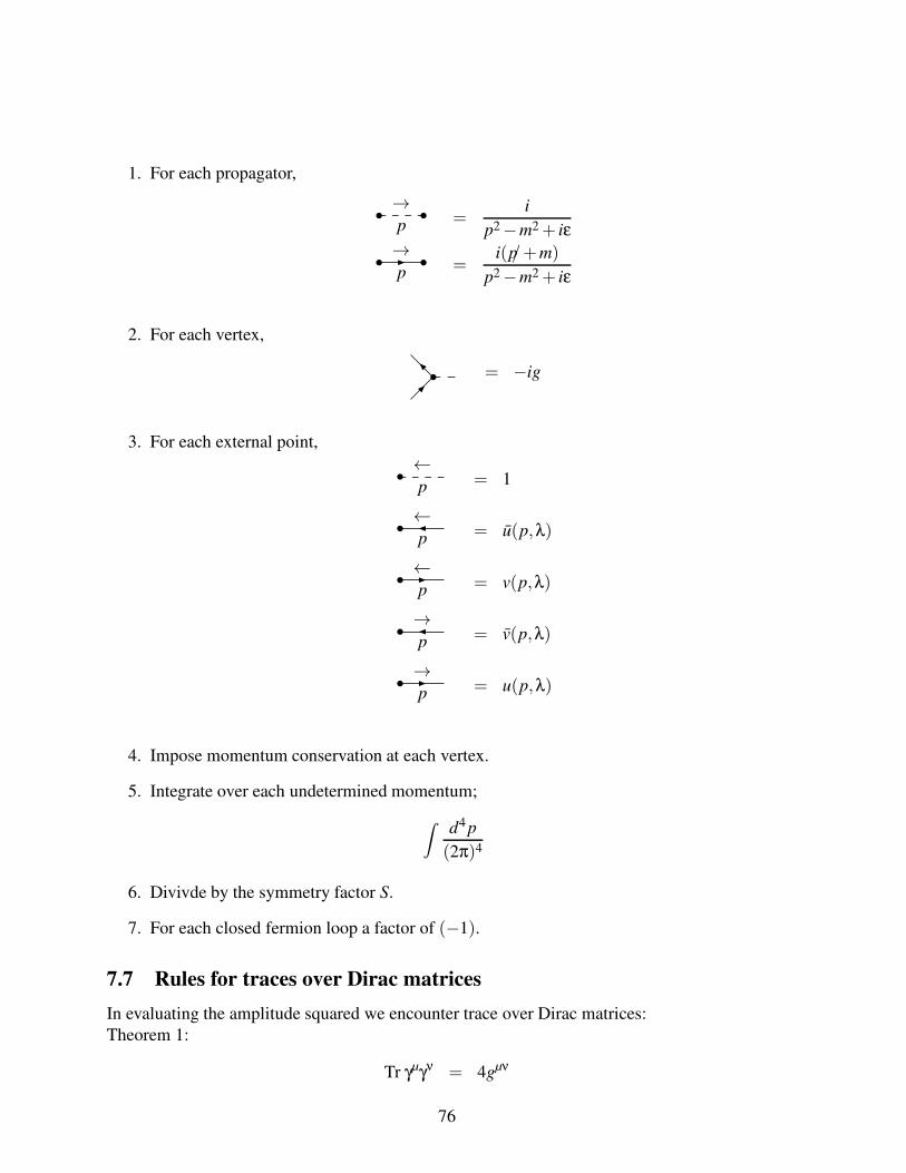
1. For each propagator,
p
→=
i
p2−m2 + iε
p
→=
i(p/+m)
p2−m2 + iε
2. For each vertex,
= −ig
3. For each external point,
p
←= 1
p
←= u(p,λ)
p
←= v(p,λ)
p
→= v(p,λ)
p
→= u(p,λ)
4. Impose momentum conservation at each vertex.
5. Integrate over each undetermined momentum;
∫d4 p
(2π)4
6. Divivde by the symmetry factor S.
7. For each closed fermion loop a factor of (−1).
7.7 Rules for traces over Dirac matrices
In evaluating the amplitude squared we encounter trace over Dirac matrices:
Theorem 1:
Tr γµγν = 4gµν
76
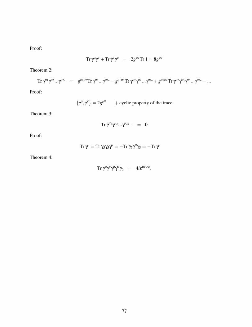
Proof:
Tr γµγν +Tr γνγµ = 2gµνTr 1 = 8gµν
Theorem 2:
Tr γµ1γµ2 ...γµ2n = gµ1µ2Tr γµ3...γµ2n−gµ1µ3Tr γµ2γµ4...γµ2n +gµ1µ4Tr γµ2γµ3γµ5 ...γµ2n− ...
Proof:
γµ,γν= 2gµν + cyclic property of the trace
Theorem 3:
Tr γµ1γµ2 ...γµ2n−1 = 0
Proof:
Tr γµ = Tr γ5γ5γµ =−Tr γ5γµγ5 =−Tr γµ
Theorem 4:
Tr γµγνγργσγ5 = 4iεµνρσ.
77
8 Quantum field theory via path integrals
Review of the canonical formalism for the quantisation of field theories: We are given a Lagrange
density
L(φ,∂µφ) = L0(φ,∂µφ)+Lint(φ,∂µφ),
which can be split into a “free” part L0 (bilinear in the fields) and a part Lint describing the inter-
actions. Each term in Lint contains at least three fields.
The momentum density conjugate to φ(x) is given by
π(x) =∂L
∂φ(x).
The Hamilton function H and the Hamiltonian H are given by
H =
∫d3x[π(x)φ(x)−L
]=
∫d3x H .
In the canonical formalism the field φ(x) and the conjugate momentum π(x) become operators.
In the Schrödinger picture the operators are time-independent. We postulate canonical (anti)-
commutation relations. For bosons we require
[φS(t0,~x), πS(t0,~y)
]= iδ3(~x−~y),
[φS(t0,~x), φS(t0,~y)
]= [πS(t0,~x), πS(t0,~y)] = 0.
For fermions we have (recall that the conjugate momentum is ∂L/∂(∂0ψ) = iψ† ):
ψS(t0,~x), iψ†S(t0,~y)
= iδ3(~x−~y),
ψS(t0,~x), ψS(t0,~y) =
iψ†S(t0,~x), iψ
†S(t0,~y)
= 0.
To change from the Schrödinger picture to the Heisenberg picture we have the formulae
φH(t,~x) = eiH(t−t0)φS(t0,~x)e−iH(t−t0),
πH(t,~x) = eiH(t−t0)πS(t0,~x)e−iH(t−t0).
We can also split the Hamiltonian into a “free” part and a piece describing the interactions:
H = H0+ Hint.
We define the field operator in the interaction picture as
φI(t,~x) = eiH0(t−t0)φS(t0,~x)e−iH0(t−t0).
78
We have the following relation between the field operators in the Heisenberg picture and the
interaction picture:
φH(x) = U†(t, t0)φI(x)U(t, t0),
where
U(t1, t0) = T
exp
−i
t1∫
t0
dt HI(t)
.
8.1 Trouble with the canonical quantisation of gauge bosons
The canonical formalism worked fine for the quantisation of spin 0 and spin 1/2 particles. Let
us now consider spin 1 particles. As a first example we consider the photon field without any
interactions with fermions. The Lagrange density is
L(Aµ,∂µAν) = −1
4FµνFµν,
where
Fµν = ∂µAν−∂νAµ.
The canonical momentum conjugate to Aµ is given by
Πµ =∂L
∂Aµ=−F0µ.
The canonical commutation relation would be given by
[Aµ(t0,~x),Πν(t0,~y)
]= igµνδ3(~x−~y).
If we set µ = ν = 0 we obtain
[A0(t0,~x),Π0(t0,~y)
]= iδ3(~x−~y).
On the other hand, we have
Π0(t0,~y) = −F00 = 0.
Thus the simple-minded application of the canonical quantisation fails. The problem is related
to the invariance of the Lagrange density under the gauge transformation
Aµ(x) → Aµ(x)+∂µΛ(x).
One possibility to circumvent the problem is to eliminate the freedom of gauge transformations
by putting constraints on the field Aµ. One adds a gauge-fixing term to the Lagrange density:
L(Aµ,∂µAν) = −1
4FµνFµν− 1
2ξ
(∂µAµ
)2
79
Remark: The Lagrange density is no longer gauge-invariant. The canonical momentum is now
given by
Πµ = −F0µ−1
ξg0µ (∂
νAν) .
The above ad-hoc recipe works fine for abelian gauge theories like QED, but fails for non-abelian
gauge theories, which are needed for the strong and weak interactions.
For a deeper understanding of the problem and its solution it is simpler to switch to a second
method for the quantisation of field theories: quantisation in the path-integral formalism.
It should be noted that with an elaborate mathematical formalism it is possible to quantise non-
abelian gauge fields also in the canonical formalism.
8.2 Path integrals
We start from the well-known Gaussian integral:
(2π)−1/2
∞∫
−∞
dy exp
(
−1
2ay2
)
= a−1/2.
This is a one-dimensional integral. We may generalise this formula to a n-dimensional integral
as follows: Let A be a real symmetric positive definite matrix. Then
(2π)−n/2
∞∫
−∞
dy1...dyn exp
(
−1
2~yT A~y
)
= (det A)−1/2 .
We recall that the exponential of a matrix A is defined by the Taylor series
exp(A) =∞
∑n=0
1
n!An
and that the logarithm of matrix A is defined is defined as a matrix such that
exp(lnA) = A.
We have the formula
ln det A = Tr lnA.
This formula is most easily proved by diagonalising the matrix A. Therefore we may re-write
our n-fold Gaussian integral as
(2π)−n/2
∞∫
−∞
dy1...dyn exp
(
−1
2~yT A~y
)
= exp
(
−1
2Tr lnA
)
.
80
We now generalise this formula in two steps: In the first step we go from a finite number of
variables y j with j ∈ 1, ...,n to an infinite countable number of variables φ j with j ∈ N. In
the second step we go from a countable number of variables φ j to an over-countable number of
variables φ(x) with x ∈ R. In this way we arrive at a path integral:∫
Dφexp
(
−1
2
∫dx
∫dy φ(x)A(x,y)φ(y)
)
= [detA(x,y)]−12
= exp
(
−1
2Tr lnA
)
The factors of (2π) on the left-hand side have been absorbed into the path integral measure Dφ.
Let us look at a simple example:
∫Dη(t) exp
−1
2
t f∫
ti
η(t)
(
− d2
dt2+ω2
)
η(t)
=
[
det
(
− d2
dt2+ω2
)]− 12
To calculate the determinant we solve the eigenvalue problem(
− d2
dt2+ω2
)
ψn(t) = λnψn(t).
One finds
λn =(
nπt f−ti
)2
+ω2,
and therefore
det
(
− d2
dt2+ω2
)
=∞
∏n=1
λn = Bsinhω
(t f − ti
)
ω(t f − ti
) ,
where B is an (infinite) constant.
Note: In practice, path integrals are never calculated explicitly !
Up to now we only considered integrals, where the argument of the exponential function was
quadratic in the integration variables. We consider now Gaussian integrals with a linear term.
For a finite number of variables one finds
(2π)−n/2
∞∫
−∞
dy1...dyn exp
(
−1
2~yT A~y+~wT~y
)
= exp
(
−1
2Tr lnA
)
exp
(1
2~wT A−1~w
)
.
Remark: A−1 exists because we assumed A to be positive definite.
Generalisation to an infinite number of components:∫
Dφexp
(
−1
2
∫dx
∫dy φ(x)A(x,y)φ(y)+
∫dx J(x)φ(x)
)
=
exp
(
−1
2Tr lnA
)
exp
(1
2
∫dx
∫dy J(x)A−1(x,y)J(y)
)
81
Let us now discuss what happens if we differentiate these formulae with respect to wi or J(x).We start with the case of a finite number of variables. Differentiation with respect to wi at ~w =~0gives:
∂
∂wi1
...∂
∂win
(2π)−n/2
∞∫
−∞
dy1...dyn exp
(
−1
2~yT A~y+~wT~y
)∣∣∣∣∣∣~w=0
=
= (2π)−n/2
∞∫
−∞
dy1...dyn yi1 ...yin exp
(
−1
2~yT A~y
)
=∂
∂wi1
...∂
∂win
exp
(
−1
2Tr lnA
)
exp
(1
2~wT A−1~w
)∣∣∣∣~w=0
In the second line we applied the differentiation under the integral, in the third line we only
substituted the result for the Gaussian integral. The main point of this formula is the equality of
the second and third line: A Gaussian integral without a term ~wT~y in the exponent, but with an
extra factor yi1...yin in front of the exponent is equal to the derivative of a Gaussian integral with
a linear term with respect to the quantities wi j.
Let us now generalise this to path integrals. We first have to generalise the ordinary derivative
to a functional derivative:
δ
δJ(y)Z [J(x)] = lim
ε→0
Z [J(x)+ εδ(x− y)]−Z [J(x)]
ε
With this definition we have the following generalisation:
∂
∂J(x1)...
∂
∂J(xn)
∫Dφexp
(
−1
2
∫dx
∫dy φ(x)A(x,y)φ(y)+
∫dx J(x)φ(x)
)∣∣∣∣J=0
=
=∫
Dφ φ(x1)...φ(xn)exp
(
−1
2
∫dx
∫dy φ(x)A(x,y)φ(y)
)
=∂
∂J(x1)...
∂
∂J(xn)exp
(
−1
2Tr lnA
)
exp
(1
2
∫dx
∫dy J(x)A−1(x,y)J(y)
)∣∣∣∣J=0
.
8.3 Transition amplitudes as path integrals
We start from the relation between Schrödinger and Heisenberg operators:
φH(t,~x) = eiH(t−t0)φS(t0,~x)e−iH(t−t0)
Here, t0 is a reference time, where φH(t0,~x) = φS(t0,~x). Let |φ(t j,~x), t〉S be a Schrödinger state,
which for t = t j is an eigenstate of the Schrödinger field operator φS(t0,~x) with eigenvalue φ(t j,~x):
φS(t0,~x)|φ(t j,~x), t j〉S = φ(t j,~x)|φ(t j,~x), t j〉S
82
Denote the corresponding Heisenberg state by
|φ(t j,~x)〉H = eiH(t−t0)|φ(t j,~x), t〉S.
|φ(t j,~x)〉H is an eigenstate of φH(t j,~x) with eigenvalue φ(t j,~x):
φH(t j,~x)|φ(t j,~x)〉H = φ(t j,~x)|φ(t j,~x)〉H .
Proof:
φH(t j,~x)|φ(t j,~x)〉H =(
eiH(t j−t0)φS(t0,~x)e−iH(t j−t0)
)(
eiH(t j−t0)|φ(t j,~x), t j〉S)
= eiH(t j−t0)φS(t0,~x)|φ(t j,~x), t j〉S = eiH(t j−t0)φ(t j,~x)|φ(t j,~x), t j〉S= φ(t j,~x)|φ(t j,~x)〉H
As a short-hand notation we write
|φk, t j〉 = |φk(t j,~x)〉H,|φk〉 = |φk(t j,~x), t j〉S.
We are interested in the transition amplitude
〈φ f , t f |φi, ti〉.
|φi, ti〉 is a state with eigenvalue φi(ti,~x) at t = ti and similar for |φ f , t f 〉. We divide the time
interval (t f − ti) into n+1 small sub-intervals with time steps at
ti, t1, t2, ..., tn, t f .
At each intermediate time step we insert a complete set of states
∫Dφ j(~x) |φ j, t j〉〈φ j, t j| = 1.
Therefore
〈φ f , t f |φi, ti〉 =∫
Dφn(~x)...∫
Dφ1(~x) 〈φ f , t f |φn, tn〉〈φn, tn|φn−1, tn−1〉...〈φ1, t1|φi, ti〉.
Let us study 〈φ j+1, t j+1|φ j, t j〉. If the time interval (t j+1− t j) is small, we have
〈φ j+1, t j+1|φ j, t j〉 =(
〈φ j+1|e−iH(t j+1−t0))(
eiH(t j−t0)|φ j, t j〉)
= 〈φ j+1|e−iH(t j+1−t j)|φ j〉≈ 〈φ j+1|1− i(t j+1− t j)H|φ j〉
Let us first consider a simple case where H is replaced by a function f (φ), which depends only
on φ, but not on π. Then
〈φ j+1| f (φ)|φ j〉 = f (φ j)〈φ j+1|φ j〉= f (φ j)δ(φ j+1−φ j)
83
We rewrite this as
〈φ j+1| f (φ)|φ j〉 = f (φ j)∫
Dπ j(~x) exp
[
i
∫d3x π j(φ j+1−φ j)
]
Note that factors of 2π are absorbed into the integral measure. Next we consider the case where
the Hamiltonian is replaced by a function g(π), which depends only on π. We introduce a com-
plete set of momentum eigenstates and obtain
〈φ j+1|g(π)|φ j〉 =
∫Dπ j(~x) g(π j)exp
[
i
∫d3x π j(φ j+1−φ j)
]
Thus if H contains only terms of the form f (φ) and g(π), its matrix element can be written as
〈φ j+1|H(φ, π)|φ j〉 =∫
Dπ j(~x) H(φ j,π j)exp
[
i
∫d3x π j(φ j+1−φ j)
]
In general this formula will not hold for arbitrary H, since the order of a product φπ matters on
the left side (where φ and π appear as operators), but not on the right side.
If this formula holds, the Hamiltonian is said to be in Weyl order. Any Hamiltonian can be
put into a Weyl order by commuting φ’s and π’s.
Assuming now Weyl order, we find
〈φ j+1|1− i(t j+1− t j)H|φ j〉 =
∫Dπ j(~x)
(1− i(t j+1− t j)H(φ j,π j)
)exp
[
i
∫d3x π j(φ j+1−φ j)
]
≈∫
Dπ j(~x) exp
[
i
(∫d3x π j(φ j+1−φ j)
)
− i(t j+1− t j)H(φ j,π j)
]
=∫
Dπ j(~x) exp
[
i(t j+1− t j)∫
d3x(π jφ j−H (φ j,π j)
)]
.
Therefore
〈φ f , t f |φi, ti〉 =
∫Dφn(~x)...
∫Dφ1(~x) 〈φ f , t f |φn, tn〉〈φn, tn|φn−1, tn−1〉...〈φ1, t1|φi, ti〉
=∫
Dφ(t,~x)∫
Dπ(t,~x) exp
[
i
∫dt
∫d3x πφ−H (φ,π)
]
.
In most cases H (φ,π) will be quadratic in π. We can then complete the square, perform a Wick
rotation and integrate over Dπ(t,~x). For example, for
H =1
2π2 +
1
2
(~∇φ)2
+V (φ) , L =1
2
(∂µφ)(∂µφ)−V (φ)
84
we have
∫Dπ(t,~x) exp
[
i
∫d4xπφ− 1
2π2− 1
2
(~∇φ)2
−V (φ)
]
=∫
Dπ(t,~x) exp
[
i
∫d4x
(
−1
2
(π− φ
)2+
1
2φ2− 1
2
(~∇φ)2
−V (φ)
)]
= N exp
[
i
∫d4x
1
2φ2− 1
2
(~∇φ)2
−V (φ)
]
= N exp
[
i
∫d4x
1
2
(∂µφ)(∂µφ)−V (φ)
]
.
One obtains
〈φ f , t f |φi, ti〉 =∫
Dφ(t,~x)∫
Dπ(t,~x) exp
[
i
∫dt
∫d3x πφ−H (φ,π)
]
=∫
Dφ(x) exp
[
i
∫d4x L
]
.
8.4 Correlation functions
In the previous section we found
〈φ f , t f |φi, ti〉 =
∫Dφ(x) exp
[
i
∫d4x L
]
.
The time interval goes from ti to t f , in all other respects this formula is manifestly Lorentz in-
variant. Any other symmetries that the Lagrangian may have are preserved by the functional
integral as long as the path integral measure is also invariant under these symmetries. This will
be important for internal symmetries related to gauge groups.
We now would like to make the next step and define quantum field theory through path inte-
grals. We have to find a functional formula to compute correlation functions like
〈Ω|T φ(x1)φ(x2)|Ω〉,
and to show its equivalence with the canonical operator formalism. Let us consider
∫Dφ(x)φ(x1)φ(x2)exp
i
T∫
−T
dt
∫d3x L(φ)
,
where the boundary conditions on the path integral are
φ(−T,~x) = φa(~x), φ(T,~x) = φb(~x).
85
We break up the functional integral as follows:∫Dφ(x) =
∫Dφ1(~x)
∫Dφ2(~x)
∫
φ(x01,~x)=φ1(~x),φ(x
02,~x)=φ2(~x)
Dφ(x)
The main functional integral∫
Dφ(x) is now constrained at times x01 and x0
2 in addition to the
endpoints −T and T . With this decomposition the extra factors φ(x1) and φ(x2) in the original
path integral become φ1(~x) and φ2(~x). If x01 < x0
2:
∫Dφ(x)φ(x1)φ(x2)exp
i
T∫
−T
dt
∫d3x L(φ)
=
=
∫Dφ1(~x)
∫Dφ2(~x)
∫
φ(x01,~x)=φ1(~x),φ(x
02,~x)=φ2(~x)
Dφ(x) φ(x1)φ(x2)exp
i
T∫
−T
dt
∫d3x L(φ)
=
∫Dφ1(~x) φ1(~x)
∫Dφ2(~x) φ2(~x)
∫
φ(x01,~x)=φ1(~x),φ(x
02,~x)=φ2(~x)
Dφ(x) exp
i
T∫
−T
dt
∫d3x L(φ)
=∫
Dφ1(~x) φ1(~x)∫
Dφ2(~x) φ2(~x) 〈φb,T |φ2,x02〉〈φ2,x
02|φ1,x
01〉〈φ1,x
01|φa,−T 〉.
Since
φH(t,~x)|φ(~x), t〉 = φ(~x)|φ(~x), t〉,we can turn the fields φi(~x) into Heisenberg operators φi(~x). Using in addition the completeness
relation ∫Dφ(~x) |φ, t〉〈φ, t| = 1,
we obtain∫Dφ1(~x) φ1(~x)
∫Dφ2(~x) φ2(~x) 〈φb,T |φ2,x
02〉〈φ2,x
02|φ1,x
01〉〈φ1,x
01|φa,−T 〉=
=∫
Dφ1(~x)∫
Dφ2(~x) 〈φb,T |φ(x2)|φ2,x02〉〈φ2,x
02|φ(x1)|φ1,x
01〉〈φ1,x
01|φa,−T 〉
=⟨φb,T
∣∣φ(x2)φ(x1)
∣∣φa,−T
⟩.
If we had the order x01 > x0
2 we would have found⟨φb,T
∣∣φ(x1)φ(x2)
∣∣φa,−T
⟩.
In summary we have shown that
∫
φ(−T,~x) = φa(~x),φ(T,~x) = φb(~x)
Dφ(x) φ(x1)φ(x2)exp
i
T∫
−T
dt
∫d3x L(φ)
=⟨φb,T
∣∣T φ(x1)φ(x2)
∣∣φa,−T
⟩.
86
If we replace the Heisenberg states by Schrödinger states
|φ(~x), t〉 = eiHt |φ(t,~x), t〉S = eiHt |φ(~x)〉,
we have⟨
φb
∣∣∣e−iHT T φ(x1)φ(x2) eiH(−T )
∣∣∣φa
⟩
.
As in the canonical operator formalism we can now send T →∞(1− iε) to project out the ground
state
e−iHT |φa〉 = ∑n
e−iEnT |n〉〈n|φa〉 → 〈Ω|φa〉 limT→∞(1−iε)
e−iE0T |Ω〉.
The phase and the overlap factor drop out if we divide by the same quantity without the field
insertions and we obtain the final formula
⟨Ω∣∣T φ(x1)φ(x2)
∣∣Ω⟩
= limT→∞(1−iε)
∫Dφ(x) φ(x1)φ(x2)exp
[i∫
d4x L(φ)]
∫Dφ(x) exp [i
∫d4x L(φ)]
.
This expresses the two-point correlation function in terms of path integrals. For higher correla-
tion functions one obtains
⟨Ω∣∣T φ(x1)...φ(xn)
∣∣Ω⟩
= limT→∞(1−iε)
∫Dφ(x) φ(x1)...φ(xn)exp
[i∫
d4x L(φ)]
∫Dφ(x) exp [i
∫d4x L(φ)]
.
Let us now introduce the “generating functional”
Z[J(x)] = N
∫Dφ(x) exp
[
i
∫d4x L(φ)+ J(x)φ(x)
]
.
We have
⟨Ω∣∣T φ(x1)...φ(xn)
∣∣Ω⟩
=(−i)n
Z[0]
δnZ[J(x)]
δJ(x1)...δJ(xn)
∣∣∣∣J=0
.
The functional Z[J] generates all Green functions:
Z[J] = Z[0]∑n
in
n!
∫d4x1...d
4xn
⟨Ω∣∣T φ(x1)...φ(xn)
∣∣Ω⟩
J(x1)...J(xn).
8.5 Fermions in the path integral formalism
8.5.1 Grassmann numbers
Ordinary number commute:
[xi,x j
]= 0.
87
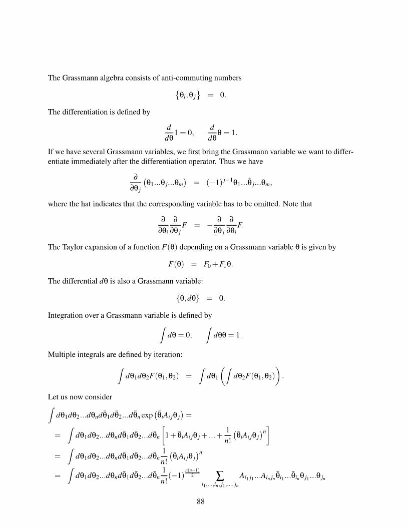
The Grassmann algebra consists of anti-commuting numbers
θi,θ j
= 0.
The differentiation is defined by
d
dθ1 = 0,
d
dθθ = 1.
If we have several Grassmann variables, we first bring the Grassmann variable we want to differ-
entiate immediately after the differentiation operator. Thus we have
∂
∂θ j
(θ1...θ j...θm
)= (−1) j−1θ1...θ j...θm,
where the hat indicates that the corresponding variable has to be omitted. Note that
∂
∂θi
∂
∂θ jF = − ∂
∂θ j
∂
∂θiF.
The Taylor expansion of a function F(θ) depending on a Grassmann variable θ is given by
F(θ) = F0 +F1θ.
The differential dθ is also a Grassmann variable:
θ,dθ = 0.
Integration over a Grassmann variable is defined by
∫dθ = 0,
∫dθθ = 1.
Multiple integrals are defined by iteration:
∫dθ1dθ2F(θ1,θ2) =
∫dθ1
(∫dθ2F(θ1,θ2)
)
.
Let us now consider∫
dθ1dθ2...dθndθ1dθ2...dθn exp(θiAi jθ j
)=
=∫
dθ1dθ2...dθndθ1dθ2...dθn
[
1+ θiAi jθ j + ...+1
n!
(θiAi jθ j
)n
]
=∫
dθ1dθ2...dθndθ1dθ2...dθn1
n!
(θiAi jθ j
)n
=∫
dθ1dθ2...dθndθ1dθ2...dθn1
n!(−1)
n(n−1)2 ∑
i1,...,in, j1,..., jn
Ai1 j1 ...Ain jn θi1...θinθ j1...θ jn
88
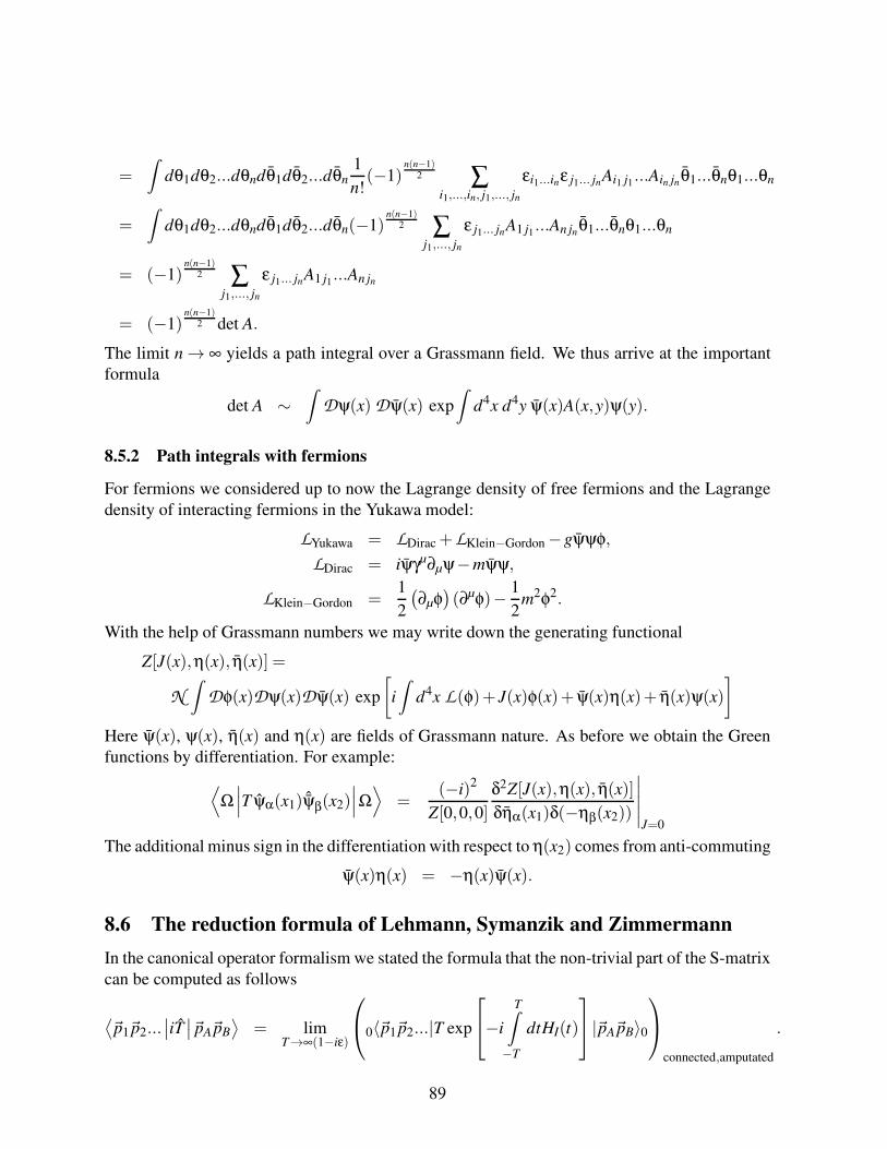
=∫
dθ1dθ2...dθndθ1dθ2...dθn1
n!(−1)
n(n−1)2 ∑
i1,...,in, j1,..., jn
εi1...inε j1... jnAi1 j1...Ain jn θ1...θnθ1...θn
=∫
dθ1dθ2...dθndθ1dθ2...dθn(−1)n(n−1)
2 ∑j1,..., jn
ε j1... jnA1 j1...An jn θ1...θnθ1...θn
= (−1)n(n−1)
2 ∑j1,..., jn
ε j1... jnA1 j1...An jn
= (−1)n(n−1)
2 det A.
The limit n→ ∞ yields a path integral over a Grassmann field. We thus arrive at the important
formula
det A ∼∫
Dψ(x) Dψ(x) exp
∫d4x d4y ψ(x)A(x,y)ψ(y).
8.5.2 Path integrals with fermions
For fermions we considered up to now the Lagrange density of free fermions and the Lagrange
density of interacting fermions in the Yukawa model:
LYukawa = LDirac +LKlein−Gordon−gψψφ,
LDirac = iψγµ∂µψ−mψψ,
LKlein−Gordon =1
2
(∂µφ)(∂µφ)− 1
2m2φ2.
With the help of Grassmann numbers we may write down the generating functional
Z[J(x),η(x), η(x)] =
N
∫Dφ(x)Dψ(x)Dψ(x) exp
[
i
∫d4x L(φ)+ J(x)φ(x)+ ψ(x)η(x)+ η(x)ψ(x)
]
Here ψ(x), ψ(x), η(x) and η(x) are fields of Grassmann nature. As before we obtain the Green
functions by differentiation. For example:
⟨
Ω∣∣∣T ψα(x1) ˆψβ(x2)
∣∣∣Ω⟩
=(−i)2
Z[0,0,0]
δ2Z[J(x),η(x), η(x)]
δηα(x1)δ(−ηβ(x2))
∣∣∣∣∣J=0
The additional minus sign in the differentiation with respect to η(x2) comes from anti-commuting
ψ(x)η(x) = −η(x)ψ(x).
8.6 The reduction formula of Lehmann, Symanzik and Zimmermann
In the canonical operator formalism we stated the formula that the non-trivial part of the S-matrix
can be computed as follows
⟨~p1~p2...
∣∣iT∣∣~pA~pB
⟩= lim
T→∞(1−iε)
0〈~p1~p2...|T exp
−i
T∫
−T
dtHI(t)
|~pA~pB〉0
connected,amputated
.
89
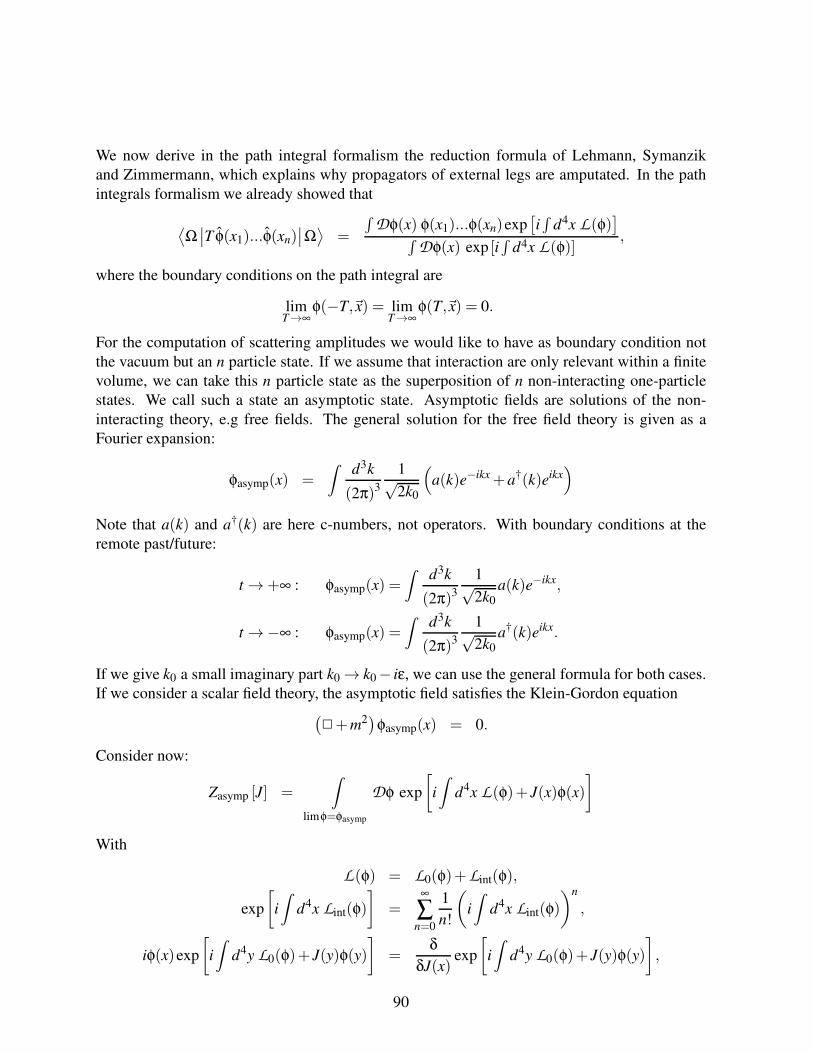
We now derive in the path integral formalism the reduction formula of Lehmann, Symanzik
and Zimmermann, which explains why propagators of external legs are amputated. In the path
integrals formalism we already showed that
⟨Ω∣∣T φ(x1)...φ(xn)
∣∣Ω⟩
=
∫Dφ(x) φ(x1)...φ(xn)exp
[i∫
d4x L(φ)]
∫Dφ(x) exp [i
∫d4x L(φ)]
,
where the boundary conditions on the path integral are
limT→∞
φ(−T,~x) = limT→∞
φ(T,~x) = 0.
For the computation of scattering amplitudes we would like to have as boundary condition not
the vacuum but an n particle state. If we assume that interaction are only relevant within a finite
volume, we can take this n particle state as the superposition of n non-interacting one-particle
states. We call such a state an asymptotic state. Asymptotic fields are solutions of the non-
interacting theory, e.g free fields. The general solution for the free field theory is given as a
Fourier expansion:
φasymp(x) =
∫d3k
(2π)3
1√2k0
(
a(k)e−ikx +a†(k)eikx)
Note that a(k) and a†(k) are here c-numbers, not operators. With boundary conditions at the
remote past/future:
t→+∞ : φasymp(x) =∫
d3k
(2π)3
1√2k0
a(k)e−ikx,
t→−∞ : φasymp(x) =∫
d3k
(2π)3
1√2k0
a†(k)eikx.
If we give k0 a small imaginary part k0→ k0− iε, we can use the general formula for both cases.
If we consider a scalar field theory, the asymptotic field satisfies the Klein-Gordon equation
(+m2
)φasymp(x) = 0.
Consider now:
Zasymp [J] =∫
limφ=φasymp
Dφ exp
[
i
∫d4x L(φ)+ J(x)φ(x)
]
With
L(φ) = L0(φ)+Lint(φ),
exp
[
i
∫d4x Lint(φ)
]
=∞
∑n=0
1
n!
(
i
∫d4x Lint(φ)
)n
,
iφ(x)exp
[
i
∫d4y L0(φ)+ J(y)φ(y)
]
=δ
δJ(x)exp
[
i
∫d4y L0(φ)+ J(y)φ(y)
]
,
90
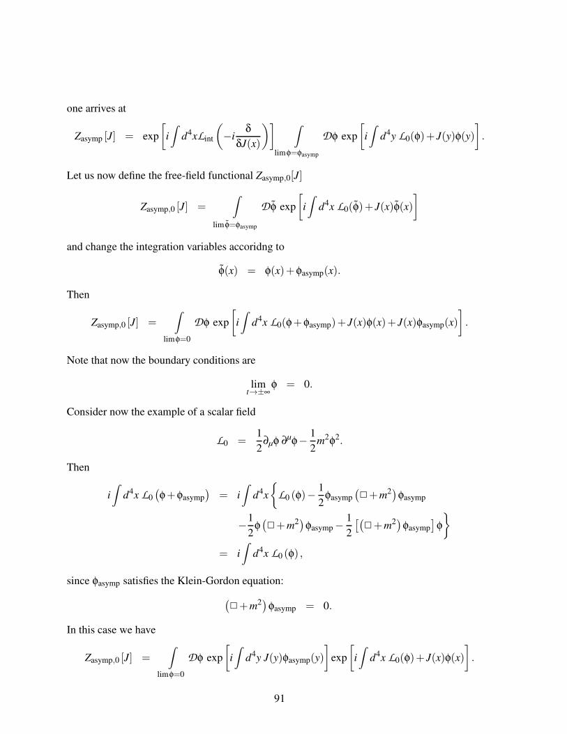
one arrives at
Zasymp [J] = exp
[
i
∫d4xLint
(
−iδ
δJ(x)
)] ∫
limφ=φasymp
Dφ exp
[
i
∫d4y L0(φ)+ J(y)φ(y)
]
.
Let us now define the free-field functional Zasymp,0[J]
Zasymp,0 [J] =
∫
lim φ=φasymp
Dφ exp
[
i
∫d4x L0(φ)+ J(x)φ(x)
]
and change the integration variables accoridng to
φ(x) = φ(x)+φasymp(x).
Then
Zasymp,0 [J] =∫
limφ=0
Dφ exp
[
i
∫d4x L0(φ+φasymp)+ J(x)φ(x)+ J(x)φasymp(x)
]
.
Note that now the boundary conditions are
limt→±∞
φ = 0.
Consider now the example of a scalar field
L0 =1
2∂µφ ∂µφ− 1
2m2φ2.
Then
i
∫d4x L0
(φ+φasymp
)= i
∫d4x
L0 (φ)−1
2φasymp
(+m2
)φasymp
−1
2φ(+m2
)φasymp−
1
2
[(+m2
)φasymp
]φ
= i
∫d4x L0 (φ) ,
since φasymp satisfies the Klein-Gordon equation:
(+m2
)φasymp = 0.
In this case we have
Zasymp,0 [J] =
∫
limφ=0
Dφ exp
[
i
∫d4y J(y)φasymp(y)
]
exp
[
i
∫d4x L0(φ)+ J(x)φ(x)
]
.
91
We now write
∫
limφ=0
Dφ exp
[
i
∫d4x L0(φ)+ J(x)φ(x)
]
= exp
[
− i
2
∫d4y d4z J(y)∆(y,z)J(z)
]
.
For the example discussed above (scalar field theory) we have
∆(x− y) =∫
d4p
(2π)4e−ip(x−y) 1
p2−m2 + iε.
Since
(x +m2
)∆(x− y) = −δ(x− y)
and
δ
δJ(x)exp
[
− i
2
∫d4y d4z J(y)∆(y,z)J(z)
]
=
−i
∫d4w ∆(x−w)J(w)exp
[
− i
2
∫d4y d4z J(y)∆(y,z)J(z)
]
,
we have
(x +m2
) δ
δJ(x)exp
[
− i
2
∫d4y d4z J(y)∆(y,z)J(z)
]
= iJ(x)exp
[
− i
2
∫d4y d4z J(y)∆(y,z)J(z)
]
.
Therefore
Zasymp [J] = exp
[∫d4x φasymp(x) ·
(x +m2
) δ
δJ(x)
]
×exp
[
i
∫d4yLint
(
−iδ
δJ(y)
)]
×∫
limφ=0
Dφ exp
[
i
∫d4z(L0(φ)+ J(z)φ(z))
]
.
Let us now define
Z [J] =
∫
limφ=0
Dφ exp
[
i
∫d4z L(φ)+ J(z)φ(z)
]
.
Define the Green functions as functional derivatives of Z[J]:
Gn(x1, ...,xn) =⟨0∣∣T φ(x1)...φ(xn)
∣∣0⟩
=(−i)n
Z[0]
δnZ [J]
δJ(x1)...δJ(xn)
∣∣∣∣J=0
92
Then
Zasymp [0] = ∑in
n!
∫d4x1...d
4xnφasymp(x1)...φasymp(xn)(x1
+m2)...(xn
+m2)
Gn(x1, ...,xn).
Define now the Fourier transform of the Green functions by
Gn(x1, ...,xn) =∫
d4p1
(2π)4...
d4pn
(2π)4e−i∑ p jx j (2π)4 δ4 (p1 + ...+ pn) Gn(p1, ..., pn)
and the truncated (amputated) Green function in momentum space by
Gntrunc(p1, ..., pn) =
(i
p21−m2
)−1
...
(i
p2n−m2
)−1
Gn(p1, ..., pn).
Then
Zasymp [0] = ∑1
n!
∫d4 p j
(2π)4(2π)4 δ4
(
∑ pk
)Gn
trunc(p1, ..., pn)
∫d4x1...d
4xne−i∑ p jx jφasymp(x1)...φasymp(xn).
Consider
∫d4x e−ipxφasymp(x) =
∫d4x e−ipx
∫d3k
(2π)3
1√2k0
[
a(k)e−ikx +a†(k)eikx]
=
∫d3k
2π√2k0
[
a(k)δ4(p+ k)+a†(k)δ4(p− k)]
For k0 > 0 and p0 > 0 only the second term contributes. For k0 > 0 and p0 < 0 only the first term
contributes. One obtains
Zasymp [0] = ∑1
n!
∫d3 p j
(2π)3
1√
|2p0|(2π)4 δ4
(
∑ pk
)Gn
trunc(p1, ..., pn)∏a(−pi)∏a†(p j).
93
9 Gauge theories
We have seen that electrodynamics can be described by a gauge potential Aµ(x).
L(Aµ,∂µAν) = −1
4FµνFµν,
where
Fµν = ∂µAν−∂νAµ.
This Lagrange density is invariant under the gauge transformation
Aµ(x) → Aµ(x)−∂µΛ(x).
We can write this gauge transformation also as
Aµ(x) →U(x)(Aµ(x)+ i∂µ
)U†(x),
with
U(x) = e−iΛ(x).
The gauge symmetry is given by a U(1) group: This is an abelian group, whose elements can be
parameterised with a coordinate ϕ as follows:
e−iϕ, 0≤ ϕ < 2π.
This is obviously a group:
e−iϕ1 · e−iϕ2 = e−i(ϕ1+ϕ2),(e−iϕ
)−1= eiϕ.
It is also a one-dimensional compact manifold (e.g. the circle line).
9.1 Lie groups und Lie algebras
A Lie group is a group G which is also an analytic manifold such that the mapping (a,b)→ ab−1
of the product manifold G×G into G is analytic.
A Lie algebra over a commutative ring K is a K-module A together with a mapping x⊗y→ [x,y]such that for x,y,z ∈ A:
[x,x] = 0,
[x, [y,z]]+ [y, [z,x]]+ [z, [x,y]] = 0.
Elements of a Lie group are written in terms of the generators as
g = exp(−iT aαa) .
94
The generators T a satisfy a Lie algebra, e.g. the commutators of generators are linear combina-
tions of the generators, i.e.
[T a,T b] = i f abcT c.
Note that in the mathematical literature the convention for the definition of the generators is usu-
ally such that no explicit factors of i appear in the formulae above. The convention used in the
physical literature (which is adopted here) ensures that the generators for the unitary groups are
hermitian matrices.
Examples of Lie groups:
- GL(n,R), GL(n,C): group of non-singular n×n matrices with n2 real parameters (GL(n,R)),respectively 2n2 real parameters (GL(n,C)).
- SL(n,R), SL(n,C): detA = 1; SL(n,R) has n2−1 real parameters; SL(n,C) has 2(n2−1) real
parameters.
- O(n) : RRT = 1.
- SO(n): RRT = 1 and detR = 1.
- U(n): UU† = 1; n2 real parameters.
- SU(n): UU† = 1 and detU = 1; n2−1 real parameters.
- Sp(n): Invariance group of
n
∑j=1
(x jy j+n− x j+ny j
).
A Lie algebra is simple if it is non-Abelian and has no non-trivial ideals.
A Lie algebra is called semi-simple if it has no non-trivial Abelian ideals.
A simple Lie algebra is also semi-simple.
Semi-simple groups are a direct product of simple groups. The compact simple Lie algebras are
An = SU(n+1),
Bn = SO(2n+1),
Cn = Sp(n),
Dn = SO(2n).
The exceptional groups are
E6,E7,E8,F4,G2.
95
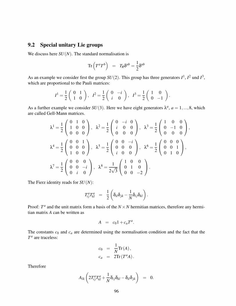
9.2 Special unitary Lie groups
We discuss here SU(N). The standard normalisation is
Tr(
T aT b)
= TRδab =1
2δab
As an example we consider first the group SU(2). This group has three generators I1, I2 und I3,
which are proportional to the Pauli matrices:
I1 =1
2
(0 1
1 0
)
, I2 =1
2
(0 −i
i 0
)
, I3 =1
2
(1 0
0 −1
)
.
As a further example we consider SU(3). Here we have eight generators λa, a = 1, ...,8, which
are called Gell-Mann matrices.
λ1 =1
2
0 1 0
1 0 0
0 0 0
, λ2 =1
2
0 −i 0
i 0 0
0 0 0
, λ3 =1
2
1 0 0
0 −1 0
0 0 0
,
λ4 =1
2
0 0 1
0 0 0
1 0 0
, λ5 =1
2
0 0 −i
0 0 0
i 0 0
, λ6 =1
2
0 0 0
0 0 1
0 1 0
,
λ7 =1
2
0 0 0
0 0 −i
0 i 0
, λ8 =1
2√
3
1 0 0
0 1 0
0 0 −2
.
The Fierz identity reads for SU(N):
T ai jT
akl =
1
2
(
δilδ jk−1
Nδi jδkl
)
.
Proof: T a and the unit matrix form a basis of the N×N hermitian matrices, therefore any hermi-
tian matrix A can be written as
A = c01+ caT a.
The constants c0 and ca are determined using the normalisation condition and the fact that the
T a are traceless:
c0 =1
NTr(A) ,
ca = 2Tr(T aA) .
Therefore
Alk
(
2T ai jT
akl +
1
Nδi jδkl−δilδ jk
)
= 0.
96
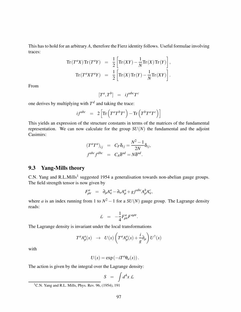
This has to hold for an arbitrary A, therefore the Fierz identity follows. Useful formulae involving
traces:
Tr(T aX)Tr(T aY ) =1
2
[
Tr(XY )− 1
NTr(X)Tr(Y )
]
,
Tr(T aXT aY ) =1
2
[
Tr(X)Tr(Y )− 1
NTr(XY )
]
.
From
[T a,T b] = i f abcT c
one derives by multiplying with T d and taking the trace:
i f abc = 2[
Tr(
T aT bT c)
−Tr(
T bT aT c)]
This yields an expression of the structure constants in terms of the matrices of the fundamental
representation. We can now calculate for the group SU(N) the fundamental and the adjoint
Casimirs:
(T aT a)i j = CFδi j =N2−1
2Nδi j,
f abc f dbc = CAδad = Nδad .
9.3 Yang-Mills theory
C.N. Yang and R.L.Mills1 suggested 1954 a generalisation towards non-abelian gauge groups.
The field strength tensor is now given by
Faµν = ∂µAa
ν−∂νAaµ +g f abcAb
µAcν,
where a is an index running from 1 to N2−1 for a SU(N) gauge group. The Lagrange density
reads:
L = −1
4Fa
µνFaµν.
The Lagrange density is invariant under the local transformations
T aAaµ(x) → U(x)
(
T aAaµ(x)+
i
g∂µ
)
U†(x)
with
U(x) = exp(−iT aθa(x)) .
The action is given by the integral over the Lagrange density:
S =∫
d4x L
1C.N. Yang and R.L. Mills, Phys. Rev. 96, (1954), 191
97

9.4 Quantisation of gauge theories
Let us examine closer the quantisation of gauge theories. The Lagrange density is given by
LQCD = −1
4Fa
µνFaµν,
with
Faµν = ∂µAa
ν−∂νAaµ +g f abcAb
µAcν.
This Lagrange density is nicely invariant under local gauge transformations
T aAaµ(x) → U(x)
(
T aAaµ(x)+
i
g∂µ
)
U†(x),
but we are not yet happy: If we try to calculate the gluon propagator we have to invert a certain
matrix and it turns out that this matrix is singular. Something is going wrong. Let´s look again
at the generating functional:
Z[J] =
∫DAa
µ(x) exp
[
i
∫d4x L +Aa
µ(x)Jµa(x)
]
The path integral is over all possible gauge field configurations, even the ones which are just
related by a gauge transformation. These configuration describe the same physics and it is suf-
ficient to count them only ones. Technically this is done as follows: Let us denote a gauge
transformation by
U(x) = exp(
−iT bθb(x))
.
The gauge transformation is therefore completely specified by the functions θb(x). We denote
by Aaµ(x,θb) the gauge field configuration obtained from Aa
µ(x) through the gauge transforamtion
U(x):
T aAaµ(x,θb) = U(x)
(
T aAaµ(x)+
i
g∂µ
)
U†(x),
Aaµ(x,θb) and Aa
µ(x) are therefore gauge-equivalent configurations. From all gauge-equivalent
configurations we are going to pick the one, which satisfies for a given Gµ and Ba(x) the equation
GµAaµ(x,θb) = Ba(x).
Let us assume that this equation gives a unique solution θb for a given Aaµ. (This is not necessarily
always fulfilled, cases where a unique solution may not exist are known as the Gribov ambiguity.)
Let~α = (α1, ...,αn) a n-dimensional vector and let the
gi = gi(α1, ..,αn), i = 1, ...,n,
98
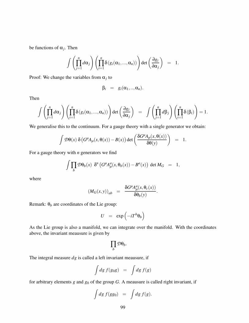
be functions of α j. Then
∫ ( n
∏j=1
dα j
)(n
∏i=1
δ(gi(α1, ...,αn))
)
det
(∂gi
∂α j
)
= 1.
Proof: We change the variables from α j to
βi = gi(α1, ..,αn).
Then
∫ ( n
∏j=1
dα j
)(n
∏i=1
δ(gi(α1, ...,αn))
)
det
(∂gi
∂α j
)
=∫ ( n
∏j=1
dβ j
)(n
∏i=1
δ(βi)
)
= 1.
We generalise this to the continuum. For a gauge theory with a single generator we obtain:
∫Dθ(x) δ
(GµAµ(x,θ(x))−B(x)
)det
(δGµAµ(x,θ(x))
δθ(y)
)
= 1.
For a gauge theory with n generators we find
∫∏
b
Dθb(x) δn(GµAa
µ(x,θb(x))−Ba(x))
det MG = 1,
where
(MG(x,y))ab =δGµAa
µ(x,θc(x))
δθb(y).
Remark: θb are coordinates of the Lie group:
U = exp(
−iT bθb
)
As the Lie group is also a manifold, we can integrate over the manifold. With the coordinates
above, the invariant meausure is given by
∏b
Dθb.
The integral measure dg is called a left invariant meausure, if
∫dg f (g0g) =
∫dg f (g)
for arbitrary elements g and g0 of the group G. A meausure is called right invariant, if
∫dg f (gg0) =
∫dg f (g).
99
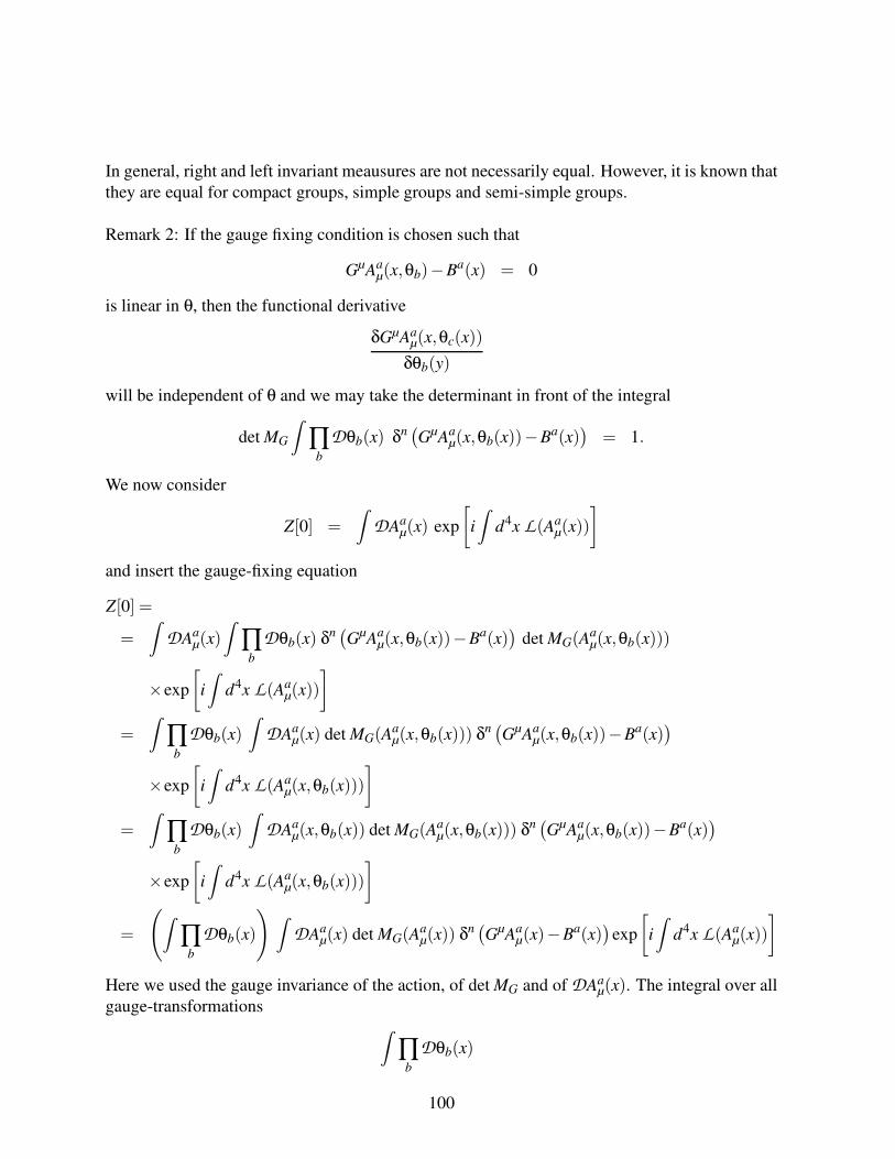
In general, right and left invariant meausures are not necessarily equal. However, it is known that
they are equal for compact groups, simple groups and semi-simple groups.
Remark 2: If the gauge fixing condition is chosen such that
GµAaµ(x,θb)−Ba(x) = 0
is linear in θ, then the functional derivative
δGµAaµ(x,θc(x))
δθb(y)
will be independent of θ and we may take the determinant in front of the integral
det MG
∫∏
b
Dθb(x) δn(GµAa
µ(x,θb(x))−Ba(x))
= 1.
We now consider
Z[0] =
∫DAa
µ(x) exp
[
i
∫d4x L(Aa
µ(x))
]
and insert the gauge-fixing equation
Z[0] =
=
∫DAa
µ(x)
∫∏
b
Dθb(x) δn(GµAa
µ(x,θb(x))−Ba(x))
det MG(Aaµ(x,θb(x)))
×exp
[
i
∫d4x L(Aa
µ(x))
]
=
∫∏
b
Dθb(x)
∫DAa
µ(x) det MG(Aaµ(x,θb(x))) δn
(GµAa
µ(x,θb(x))−Ba(x))
×exp
[
i
∫d4x L(Aa
µ(x,θb(x)))
]
=∫
∏b
Dθb(x)∫
DAaµ(x,θb(x)) det MG(A
aµ(x,θb(x))) δn
(GµAa
µ(x,θb(x))−Ba(x))
×exp
[
i
∫d4x L(Aa
µ(x,θb(x)))
]
=
(∫∏
b
Dθb(x)
) ∫DAa
µ(x) det MG(Aaµ(x)) δn
(GµAa
µ(x)−Ba(x))
exp
[
i
∫d4x L(Aa
µ(x))
]
Here we used the gauge invariance of the action, of det MG and of DAaµ(x). The integral over all
gauge-transformations∫
∏b
Dθb(x)
100
is the just an irrelevant prefactor, which we neglect in the following. We then obtain
Z[0] =
∫DAa
µ(x) det MG(Aaµ(x)) δn
(GµAa
µ(x)−Ba(x))
exp
[
i
∫d4x L(Aa
µ(x))
]
This functional still depends on Ba(x). As we are not interested in any particular choice of Ba(x),we average over Ba(x) with weight
exp
(
− i
2ξ
∫d4x(Ba(x)Ba(x))
)
and obtain
∫DBa(x) Z[0]exp
(
− i
2ξ
∫d4x(Ba(x)Ba(x))
)
=
=∫
DBa(x)∫
DAaµ(x) det MG δn
(GµAa
µ(x)−Ba(x))
exp
[
i
∫d4x L(Aa
µ(x))−1
2ξBa(x)Ba(x)
]
=∫
DAaµ(x) det MG exp
[
i
∫d4x L(Aa
µ(x))−1
2ξ
(GµAa
µ(x))(GνAν a(x))
]
.
We now consider as new generating functional
Z[J] =∫
DAaµ(x) det MG exp
[
i
∫d4x L(Aa
µ(x))−1
2ξ
(GµAa
µ(x))(GνAν a(x))+Aa
µ(x)Jµa(x)
]
.
We observe that Z[J] contains a term we could expect from a naive fixing of the gauge
− 1
2ξ
(GµAa
µ(x))(GνAν a(x)) .
In addition, the determinant
det MG
appears in front of the exponent.
Various gauges are:
• Lorenz gauge or covariant gauge: Gµ = ∂µ.
(MG(x,y))ab =
(
δab−g f abc∂µAc
µ
)
δ4(x− y)
• Coulomb gauge: Gµ = (0,~∇).
(MG(x,y))ab =
(
δab∇2−g f abc~Ac~∇)
δ4(x− y)
101
• Axial gauge: Gµ = nµ, where nµ is a constant four-vector.
(MG(x,y))ab =
(
δabn ·∂−g f abcn ·Ac)
δ4(x− y)
We would like to exponentiate the determinant. In the treatment of fermions within the path-
integral formalism we had the formula
det A ∼∫
Dψ(x) Dψ(x) exp
∫d4x d4y ψ(x)A(x,y)ψ(y).
We write this as
det A =
∫Dψ(x) Dψ(x) exp−i
∫d4x d4y ψ(x)A(x,y)ψ(y).
Applying this to det MG:
det MG =
∫Dcb(x) D ca(x) exp
(
i
∫d4x ca(x)
(
−MabG
)
cb(x)
)
.
Specialising to the covariant gauge Gµ = ∂µ one obtains
det MG =
∫Dcb(x) D ca(x) exp
(
i
∫d4x ca(x)
(
−δab+g f abc∂µAc
µ
)
cb(x)
)
=
∫Dcb(x) D ca(x) exp
(
i
∫d4x ca(x)
(
−∂µDabµ
)
cb(x)
)
,
where
Dabµ = δab∂µ−g f abcAc
µ
is the covariant derivative. In the Lorenz gauge we obtain finally
Z[J,ξ, ξ] =
∫DAa
µ(x)
∫Dcb(x) D ca(x)
exp
[
i
∫d4x L(Aa
µ(x))−1
2ξ
(∂µAa
µ(x))(∂νAa
ν(x))+ ca(x)(
−∂µDabµ
)
cb(x)
+Aaµ(x)J
µa(x)+ ca(x)ξa(x)+ ξa(x)c
b(x)]
.
The quantity
LGF = − 1
2ξ
(∂µAa
µ
)(∂νAa
ν)
is called the gauge-fixing term, the quantity
LFP = −ca∂µDabµ cb
the Faddeev-Popov term.
102
9.5 The Lagrange density for the fermion sector
Example: The Lagrange density for a free electron (e.g. no interactions) is given by
LF = ψ(iγµ∂µ−me)ψ.
We are now looking for a Lagrange density for the fermionic sector, which remains invariant
under gauge transformations. Recall that under a gauge transformation a fermion field ψi(x)transforms as
ψi(x)→Ui j(x)ψ j(x), Ui j(x) = exp(−iT aθa(x)) ,
ψi(x)→ ψ j(x)U†ji(x).
θa(x) depends on the space-time coordinates x. For an infinitessimal gauge transformation we
have
ψi(x) → (1− iT aθa(x))ψ j(x).
We immediately see that a fermion mass term
−mψ(x)ψ(x)
is invariant under gauge transformations. (Note however that in the standard model the fermion
masses are generated through the Yukawa couplings to the Higgs field.) But the term involving
derivatives is not gauge invariant:
iψ(x)γµ∂µψ(x) → iψ(x)U†(x)γµ∂µ (U(x)ψ(x)) = iψ(x)γµ∂µψ(x)+ iψ(x)γµ(
U†(x)∂µU(x))
ψ(x)︸ ︷︷ ︸
extra
.
The solution comes in the form of the covariant derivative
Dµ = ∂µ− igT aAaµ(x),
where the gauge field transforms as
T aAaµ(x) → U(x)
(
T aAaµ(x)+
i
g∂µ
)
U†(x).
Then the combination
iψ(x)γµDµψ(x) = iψ(x)γµ(∂µ− igT aAa
µ(x))
ψ(x)
→ iψ(x)U†(x)γµ
[
∂µ− igU(x)
(
T aAaµ(x)+
i
g∂µ
)
U†(x)
]
U(x)ψ(x)
= iψ(x)γµ∂µψ(x)+ iψ(x)γµ(
U†(x)∂µU(x))
ψ(x)
+gψ(x)γµT aAaµ(x)ψ(x)+ iψ(x)γµ
[(
∂µU†(x))
U(x)]
ψ(x)
is invariant.
The Lagrange density for the fermion sector:
Lfermions = ∑fermions
ψ(x)(iγµDµ−m
)ψ(x).
103
9.6 Feynman rules for QED and QCD
Expanding the Lagrange density into terms bilinear in the fields and interaction terms. As an
example consider the gluonic part of the Lagrange density:
LQCD = −1
4Fa
µνFaµν− 1
2ξ(∂µAa
µ)2 +LFP +Lfermions
where
Faµν = ∂µAa
ν−∂νAaµ +g f abcAb
µAcν.
This yields
LQCD = −1
4
(∂µAa
ν−∂νAaµ
)2− 1
2ξ(∂µAa
µ)2
−g f abc(∂µAa
ν
)AbµAcν− 1
4g2(
f eabAaµAb
ν
)(
f ecdAcµAdν)
+LFP +Lfermions.
Terms bilinear in the fields define the propagators. Terms with three or more fields define inter-
action vertices.
For QED (photons and electrons) the Lagrange density is given by
LQED = ψ(i∂/−me)ψ−1
4
(∂µAν−∂νAµ
)2− 1
2ξ(∂µAµ)
2 + eψγµAµψ.
In the QED case, the Faddeey-Popov ghosts have no interactions and behave as non-interacting
free particles. We may ignore them in the QED case.
9.6.1 Propagators
Terms bilinear in the fields yield propagators. Consider
Lbilinear(x) =
1
2φi(x)P
boson,reali j (x)φ j(x)+χ∗i (x)P
boson,complexi j (x)χ j(x)+ ψi(x)P
fermioni j (x)ψ j(x),
where φi denotes a set of real boson fields (one degree of freedom), χi denotes a set of complex
boson fields (two degrees of freedom), and ψi denotes a set of fermion fields. The boson fields
may be scalar or vector fields. P is a matrix operator that may contain derivatives and must have
an inverse. P is taken to be a hermitian operator (real symmetric operator in the case of real
boson fields):
P† = P
104
Define the inverse of P by
∑j
Pi j(x)P−1jl (x− y) = δilδ
4(x− y),
and its Fourier transform by
P−1i j (x) =
∫d4k
(2π)4e−ik·xP−1
i j (k).
Then the propagator is given by
∆F(k)i j =
∫d4xeik·x〈0|T (φi(x)φ j(0)|0〉= i
(P−1(k)
)
i j.
The propagator of a scalar particle:
From
P(x) = −−m2
we found already
P−1(k) =1
k2−m2
and therefore
∆F(k) =i
k2−m2.
The propagator of a fermion: We start from
P(x) = i∂/−m.
Then
(i∂/x−m)
∫d4k
(2π)4e−ik·(x−y)P−1(k) =
∫d4k
(2π)4(k/−m)e−ik·(x−y)P−1(k) =
∫d4k
(2π)4e−ik·(x−y).
Therefore
(k/−m) P−1(k) = 1
and
∆F(k) = ik/+m
k2−m2.
105
The propagator of a gauge boson:
In Lorentz gauge the gauge-fixing term is given by
LGF = − 1
2ξ(∂µAµ)
2
and therefore
P(x) = gµν−(
1− 1
ξ
)
∂µ∂ν.
Then
P(x)∫
d4k
(2π)4e−ik·(x−y)P−1(k) =
∫d4k
(2π)4k2
(
−gµν +
(
1− 1
ξ
)kµkν
k2
)
e−ik·(x−y)P−1(k).
We have for
Mµν =−gµν +
(
1− 1
ξ
)kµkν
k2and Nµν =−gµν +(1−ξ)
kµkν
k2
the following relation:
MµλNλν = g νµ .
Therefore
∆F(k) =i
k2
(
−gµν +(1−ξ)kµkν
k2
)
.
9.6.2 Vertices
A general term in Lint(x) has the form
Lint(x) =∫
d4x1...d4xnαi1...in(x,x1, ...,xn)φi1(x1)...φin(xn).
For the vertex we define
αi1...in(x,x1, ...,xn) =∫
d4k1
(2π)4...
d4kn
(2π)4e−ik1(x−x1)−...−ikn(x−xn)αi1...in(k1, ...,kn).
α contains a factor ik jµ for every derivative ∂/∂x jµ acting on a field with argument x j. The vertex
is then given by
I(k1, ...,kn) = i ∑permutations
(−1)Pαi1...in(k1, ...,kn).
106
The summations are over all permutations of indices and momenta. The momenta are taken to
flow inward.
Example: The quark-gluon vertex
Lint = gψiγµ(T a)i jAaµψ j =
∫d4x1
∫d4x2
∫d4x3δ4(x− x1)δ
4(x− x2)δ4(x− x3)
×[gγµ(T a)i j
]ψi(x1)ψ
j(x2)Aaµ(x3).
Then
α(k1,k2,k3) = gγµ(T a)i j
and
I = igγµ(T a)i j.
Example 2: The three-gluon vertex
Lint =−g f abc(∂µAa
ν
)AbµAcν
=∫
d4x1
∫d4x2
∫d4x3δ4(x− x1)δ
4(x− x2)δ4(x− x3)
(
−g f abc)
∂νx1
gµλAaµ(x1)A
bν(x2)A
cλ(x3)
=∫
d4x1
∫d4x2
∫d4x3Aa
µ(x1)Abν(x2)A
cλ(x3)g f abcgµλ∂ν
x1δ4(x− x1)δ
4(x− x2)δ4(x− x3).
Therefore
α(x,x1,x2,x3) = g f abcgµλ∂νx1
δ4(x− x1)δ4(x− x2)δ
4(x− x3)
= g f abcgµλ∂νx1
∫d4k1
(2π)4
∫d4k2
(2π)4
∫d4k3
(2π)4e−ik1(x−x1)e−ik2(x−x2)e−ik3(x−x3)
=
∫d4k1
(2π)4
∫d4k2
(2π)4
∫d4k3
(2π)4g f abcgµλikν
1e−ik1(x−x1)e−ik2(x−x2)e−ik3(x−x3)
and
α(k1,k2,k3) = g f abcgµλikν1.
Then
I = i ∑permutations
α(k1,k2,k3) = g f abc[(k2− k3)µgνλ+(k3− k1)νgλµ +(k1− k2)λgµν
].
9.6.3 List of Feynman rules
Propagators:
107

The propagators for the gauge bosons are in the Feynman gauge (ξ = 1).
gauge bosons gluon Aaµ−igµν
k2 δab
photon Aµ−igµν
k2
fermions quarks ψi ip/+m
p2−m2 δi j
leptons ψ ip/+m
p2−m2
ghosts ca ik2 δab
Vertices:
Quark-gluon-vertex:
igγµT ai j
3-gluon-vertex:
k1,µ,a
k2,ν,bk3,λ,c
g f abc[(k2− k3)µgνλ +(k3− k1)νgλµ +(k1− k2)λgµν
]
4-gluon-vertex:
µ,a
ν,bλ,c
ρ,d
108
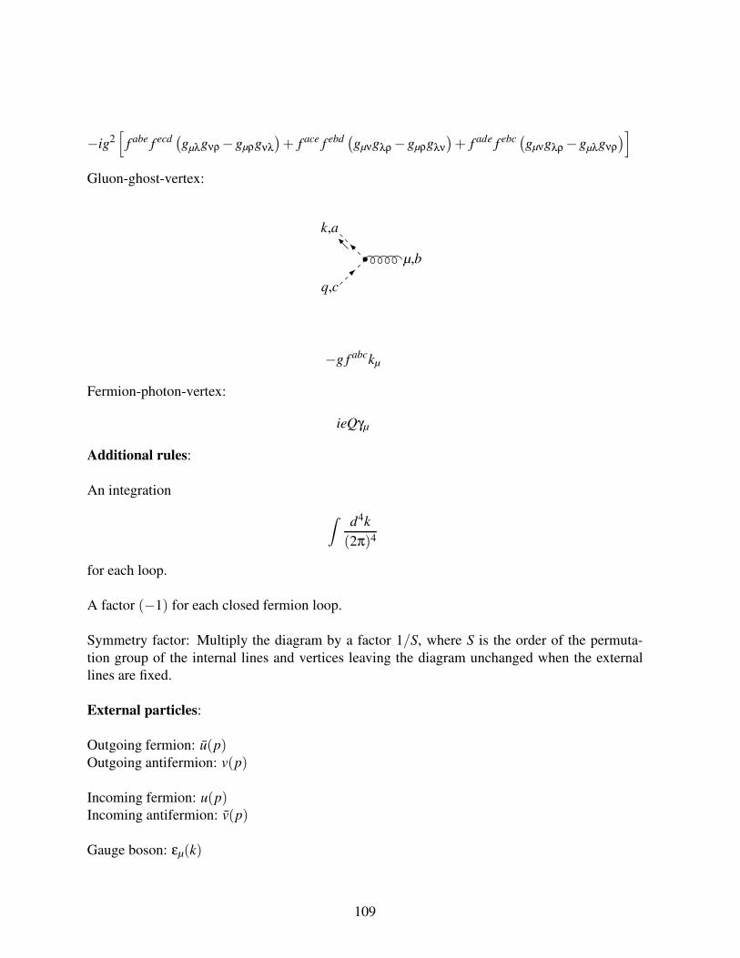
−ig2[
f abe f ecd(gµλgνρ−gµρgνλ
)+ f ace f ebd
(gµνgλρ−gµρgλν
)+ f ade f ebc
(gµνgλρ−gµλgνρ
)]
Gluon-ghost-vertex:
µ,b
q,c
k,a
−g f abckµ
Fermion-photon-vertex:
ieQγµ
Additional rules:
An integration
∫d4k
(2π)4
for each loop.
A factor (−1) for each closed fermion loop.
Symmetry factor: Multiply the diagram by a factor 1/S, where S is the order of the permuta-
tion group of the internal lines and vertices leaving the diagram unchanged when the external
lines are fixed.
External particles:
Outgoing fermion: u(p)Outgoing antifermion: v(p)
Incoming fermion: u(p)Incoming antifermion: v(p)
Gauge boson: εµ(k)
109
Polarisation sums:
∑λ
u(p,λ)u(p,λ) = p/+m,
∑λ
v(p,λ)v(p,λ) = p/−m,
∑λ
ε∗µ(k,λ)εν(k,λ) = −gµν +kµnν +nµkν
kn−n2 kµkν
(kn)2.
Here nµ is an arbitrary four vector. The dependence on nµ cancels in gauge-invariant quantities.
Using Weyl spinors, a convenient choice of polarisation vectors for the gauge bosons is given by
ε+µ (k,q) =〈q−|γµ|k−〉√
2〈qk〉,
ε−µ (k,q) =〈q+ |γµ|k+〉√
2 [kq],
where qµ is an arbitrary light-like reference momentum. The dependence on qµ cancels in gauge-
invariant quantities. The polarisation vectors satisfy:
ε±µ (k,q)kµ = 0,
ε±µ (k,q)qµ = 0.
ε+ ·(ε+)∗
= ε− ·(ε−)∗
=−1,
ε+ ·(ε−)∗
= 0.
(ε+µ)∗
= ε−µ .
9.7 Colour decomposition
Amplitudes in QCD may be decomposed into group-theoretical factors (carrying the colour struc-
tures) multiplied by kinematic functions called partial amplitudes. These partial amplitudes do
not contain any colour information and are gauge-invariant objects. Partial amplitudes may be
decomposed further into primitive amplitudes.
The colour decomposition is obtained by replacing the structure constants f abc by
i f abc = 2[
Tr(
T aT bT c)
−Tr(
T bT aT c)]
110
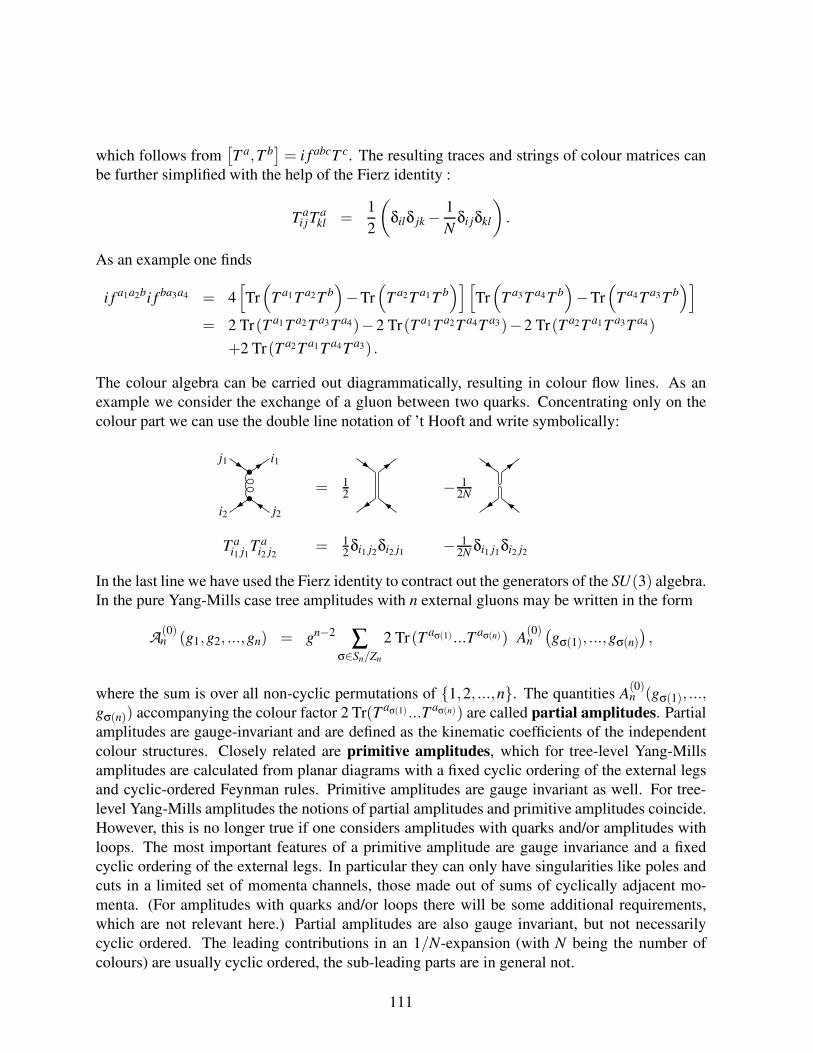
which follows from[T a,T b
]= i f abcT c. The resulting traces and strings of colour matrices can
be further simplified with the help of the Fierz identity :
T ai jT
akl =
1
2
(
δilδ jk−1
Nδi jδkl
)
.
As an example one finds
i f a1a2bi f ba3a4 = 4[
Tr(
T a1T a2T b)
−Tr(
T a2T a1T b)][
Tr(
T a3T a4T b)
−Tr(
T a4T a3T b)]
= 2 Tr(T a1T a2T a3T a4)−2 Tr(T a1T a2T a4T a3)−2 Tr(T a2T a1T a3T a4)
+2 Tr(T a2T a1T a4T a3) .
The colour algebra can be carried out diagrammatically, resulting in colour flow lines. As an
example we consider the exchange of a gluon between two quarks. Concentrating only on the
colour part we can use the double line notation of ’t Hooft and write symbolically:
j1
i2
i1
j2
= 12
− 12N
T ai1 j1
T ai2 j2
= 12δi1 j2δi2 j1 − 1
2Nδi1 j1δi2 j2
In the last line we have used the Fierz identity to contract out the generators of the SU(3) algebra.
In the pure Yang-Mills case tree amplitudes with n external gluons may be written in the form
A(0)n (g1,g2, ...,gn) = gn−2 ∑
σ∈Sn/Zn
2 Tr(T aσ(1) ...T aσ(n)) A(0)n
(gσ(1), ...,gσ(n)
),
where the sum is over all non-cyclic permutations of 1,2, ...,n. The quantities A(0)n (gσ(1), ...,
gσ(n)) accompanying the colour factor 2 Tr(T aσ(1) ...T aσ(n)) are called partial amplitudes. Partial
amplitudes are gauge-invariant and are defined as the kinematic coefficients of the independent
colour structures. Closely related are primitive amplitudes, which for tree-level Yang-Mills
amplitudes are calculated from planar diagrams with a fixed cyclic ordering of the external legs
and cyclic-ordered Feynman rules. Primitive amplitudes are gauge invariant as well. For tree-
level Yang-Mills amplitudes the notions of partial amplitudes and primitive amplitudes coincide.
However, this is no longer true if one considers amplitudes with quarks and/or amplitudes with
loops. The most important features of a primitive amplitude are gauge invariance and a fixed
cyclic ordering of the external legs. In particular they can only have singularities like poles and
cuts in a limited set of momenta channels, those made out of sums of cyclically adjacent mo-
menta. (For amplitudes with quarks and/or loops there will be some additional requirements,
which are not relevant here.) Partial amplitudes are also gauge invariant, but not necessarily
cyclic ordered. The leading contributions in an 1/N-expansion (with N being the number of
colours) are usually cyclic ordered, the sub-leading parts are in general not.
111
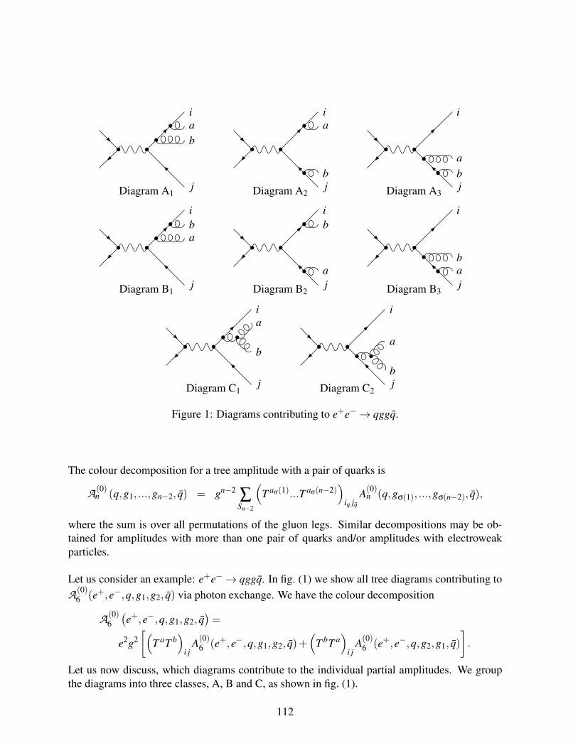
Diagram A1
i
a
b
j Diagram A2
i
a
b
j Diagram A3
i
a
b
j
Diagram B1
i
b
a
j Diagram B2
i
b
a
j Diagram B3
i
b
a
j
Diagram C1
i
a
b
j Diagram C2
i
a
b
j
Figure 1: Diagrams contributing to e+e−→ qggq.
The colour decomposition for a tree amplitude with a pair of quarks is
A(0)n (q,g1, ...,gn−2, q) = gn−2 ∑
Sn−2
(
T aσ(1)...T aσ(n−2))
iq jqA(0)n (q,gσ(1), ...,gσ(n−2), q),
where the sum is over all permutations of the gluon legs. Similar decompositions may be ob-
tained for amplitudes with more than one pair of quarks and/or amplitudes with electroweak
particles.
Let us consider an example: e+e−→ qggq. In fig. (1) we show all tree diagrams contributing to
A(0)6 (e+,e−,q,g1,g2, q) via photon exchange. We have the colour decomposition
A(0)6
(e+,e−,q,g1,g2, q
)=
e2g2
[(
T aT b)
i jA(0)6 (e+,e−,q,g1,g2, q)+
(
T bT a)
i jA(0)6 (e+,e−,q,g2,g1, q)
]
.
Let us now discuss, which diagrams contribute to the individual partial amplitudes. We group
the diagrams into three classes, A, B and C, as shown in fig. (1).
112

Colour factor of diagrams of class A j:(
T aT b)
i j
Colour factor of diagrams of class B j:(
T bT a)
i j
Colour factor of diagrams of class C j:
T ci ji f abc = 2T c
i j
(
Tr T aT bT c− Tr T bT aT c)
=(
T aT b)
i j−(
T bT a)
i j
Note that the third colour structure is a linear combination of the first two and diagrams from
class C contribute to both partial amplitudes.
The two colour factors (T aT b)i j and (T bT a)i j are orthogonal to leading order in 1/N:
(
T aikT b
k j
)†(
T aikT b
k j
)
= Tr T aT aT bT b =
(1
2
)2 (N2−1)2
N=
1
4N3 +O(N)
(
T aikT b
k j
)†(
T bikT a
k j
)
= Tr T aT bT aT b =−(
1
2
)2N2−1
N= O(N)
Orthogonality to leading order in 1/N can be used to prove that the partial amplitudes are indi-
vidually gauge invariant: The full amplitude A(0)n is gauge invariant and the partial amplitudes
A(0)n do not depend on N, therefore multiplying the colour decomposition by an appropriate string
of colour matrices and taking the N → ∞-limit shows that the individual partial amplitudes are
gauge invariant.
We already mentioned that for tree-level amplitudes with zero or one quark-antiquark pair the
notions of partial amplitudes and primitive amplitudes coincide. Primitive amplitudes are calcu-
lated from planar diagrams with a fixed cyclic ordering of the external legs and cyclic-ordered
Feynman rules. The cyclic-ordered Feynman rules are obtained from the standard Feynman
rules by extracting from each formula the coupling constant and by taking the coefficient of the
cyclic-ordered colour part. Let us now list the cyclic-ordered Feynman rules. The propagators
for quark, gluon and ghost particles are given by
= ip/+m
p2−m2,
=−igµν
p2,
=i
p2.
113
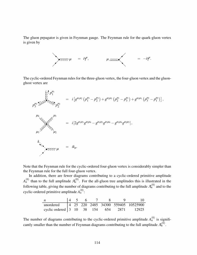
The gluon prpagator is given in Feynman gauge. The Feynman rule for the quark-gluon vertex
is given by
µ = iγµ, µ = −iγµ.
The cyclic-ordered Feynman rules for the three-gluon vertex, the four-gluon vertex and the gluon-
ghost vertex are
pµ1
1
pµ2
2pµ3
3
= i[gµ1µ2
(p
µ3
1 − pµ3
2
)+gµ2µ3
(p
µ1
2 − pµ1
3
)+gµ3µ1
(p
µ2
3 − pµ2
1
)],
µ1
µ2µ3
µ4
= i [2gµ1µ3gµ2µ4−gµ1µ2gµ3µ4−gµ1µ4gµ2µ3 ] ,
µ
k
= ikµ.
Note that the Feynman rule for the cyclic-ordered four-gluon vertex is considerably simpler than
the Feynman rule for the full four-gluon vertex.
In addition, there are fewer diagrams contributing to a cyclic-ordered primitive amplitude
A(0)n than to the full amplitude A
(0)n . For the all-gluon tree amplitudes this is illustrated in the
following table, giving the number of diagrams contributing to the full amplitude A(0)n and to the
cyclic-ordered primitive amplitude A(0)n :
n 4 5 6 7 8 9 10
unordered 4 25 220 2485 34300 559405 10525900
cyclic ordered 3 10 38 154 654 2871 12925
The number of diagrams contributing to the cyclic-ordered primitive amplitude A(0)n is signifi-
cantly smaller than the number of Feynman diagrams contributing to the full amplitude A(0)n .
114
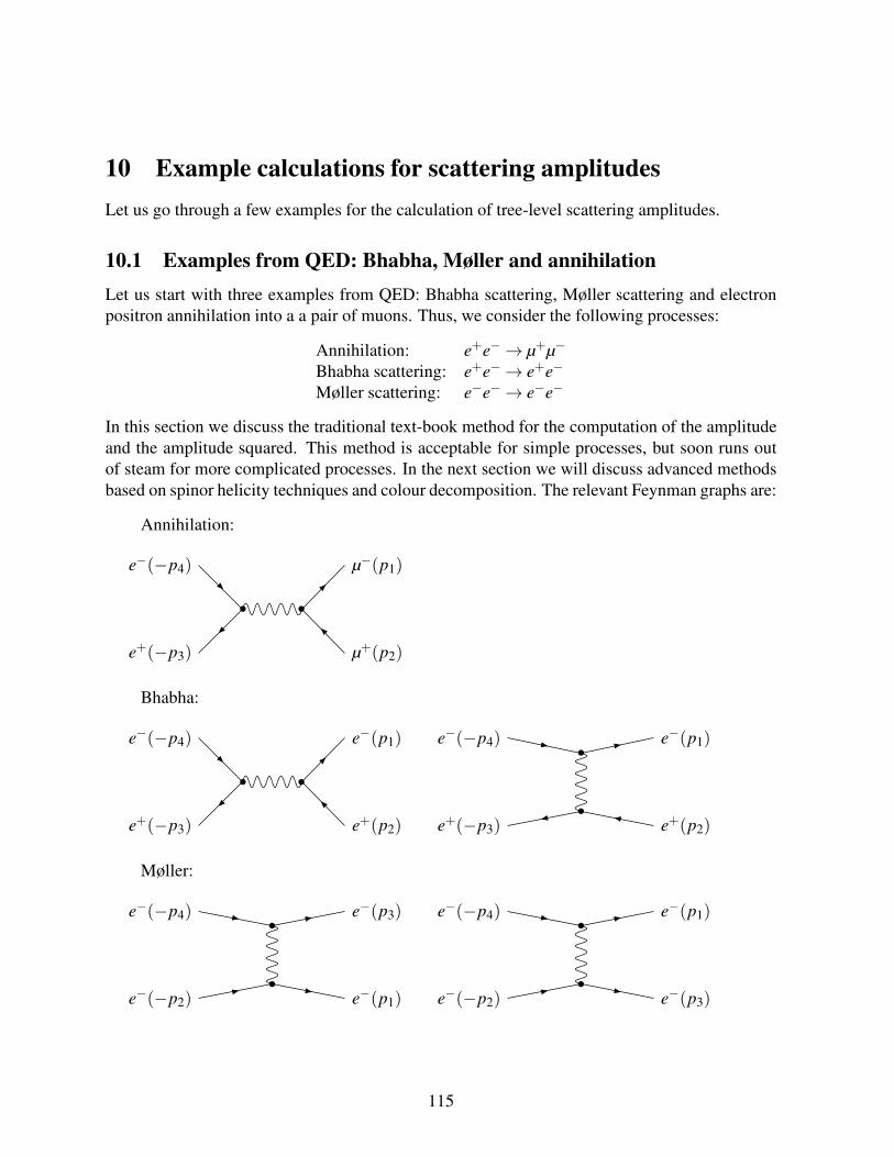
10 Example calculations for scattering amplitudes
Let us go through a few examples for the calculation of tree-level scattering amplitudes.
10.1 Examples from QED: Bhabha, Møller and annihilation
Let us start with three examples from QED: Bhabha scattering, Møller scattering and electron
positron annihilation into a a pair of muons. Thus, we consider the following processes:
Annihilation: e+e−→ µ+µ−
Bhabha scattering: e+e−→ e+e−
Møller scattering: e−e−→ e−e−
In this section we discuss the traditional text-book method for the computation of the amplitude
and the amplitude squared. This method is acceptable for simple processes, but soon runs out
of steam for more complicated processes. In the next section we will discuss advanced methods
based on spinor helicity techniques and colour decomposition. The relevant Feynman graphs are:
Annihilation:
e+(−p3)
e−(−p4)
µ+(p2)
µ−(p1)
Bhabha:
e+(−p3)
e−(−p4)
e+(p2)
e−(p1)
e+(−p3)
e−(−p4)
e+(p2)
e−(p1)
Møller:
e−(−p2)
e−(−p4)
e−(p1)
e−(p3)
e−(−p2)
e−(−p4)
e−(p3)
e−(p1)
115
Let us start with the lowest order amplitude for the annihilation process. We denote this ampli-
tude by
A(p1, p2, p3, p4).
It is convenient to take all momenta as outgoing, e.g. to consider the process
/0 → p1 + p2 + p3 + p4.
Energy-momentum conservation reads then
p1 + p2 + p3 + p4 = 0.
At high energies we may neglect the fermion masses. Then there is no difference between the
diagram for the annihilation process and the first diagram for Bhabha scattering. The second
diagram for Bhabha scattering is obtained by exchanging 2↔ 4. Therefore we have
ABhabha = A(p1, p2, p3, p4)−A(p1, p4, p3, p1)
The minus sign comes from the exchange of two fermions. p1 and p2 are the momenta of the final
state particles, −p3 and −p4 are the momenta of the initial state particles. For Møller scattering
one has the same formula:
AMoller = A(p1, p2, p3, p4)−A(p1, p4, p3, p1),
the difference corresponds only to the assignment of initial and final state momenta: For Møller
scattering p1 and p3 denote the final state momenta, −p2 and −p4 denote the initial state mo-
menta.
Let us now calculate the amplitude for the annihilation process. Using the Feynman rules we
obtain
A(p1, p2, p3, p4) = u(p1)(−ieγµ)v(p2)−igµν
(p1 + p2)2
u(p3)(−ieγν)v(p4)
=ie2
(p1 + p2)2[u(p1)γ
µv(p2)][u(p3)γµv(p4)
]
What we actually need is the amplitude squared, summed over all spins:
∑spin
|A |2 =
= ∑λ1,λ2,λ3,λ4
∣∣∣∣∣
ie2
(p1 + p2)2
∣∣∣∣∣
2([u(p1)γ
µv(p2)][u(p3)γµv(p4)
])([u(p1)γ
νv(p2)] [u(p3)γνv(p4)])∗
=e4
s212
∑λ1,λ2,λ3,λ4
[u(p1)γµv(p2)]
[u(p3)γµv(p4)
][v(p2)γ
νu(p1)] [v(p4)γνu(p3)]
=e4
s212
∑λ1,λ2,λ3,λ4
[u(p1)γµv(p2)] [v(p2)γ
νu(p1)][u(p3)γµv(p4)
][v(p4)γνu(p3)]
116
We can now use the polarisation sums
∑λ
u(p)u(p) = ∑λ
u(p)u(p) = p/
and obtain
∑spin
|A |2 =e4
s212
(Tr p/1γµp/2γν)(Tr p/3γµp/4γν
)
We now have to work out the traces over the Dirac matrices. We recall
Tr γµγν = 4gµν,
Tr γµ1γµ2 ...γµ2n = gµ1µ2Tr γµ3...γµ2n−gµ1µ3Tr γµ2γµ4 ...γµ2n +gµ1µ4Tr γµ2γµ3γµ5...γµ2n− ...,
Tr γµ1γµ2 ...γµ2n−1 = 0,
Tr γµγνγργσγ5 = 4iεµνρσ.
With the help of these theorems we find
Tr p/1γµ p/2γν = 2s12
(
−gµν +p
µ1 pν
2 + pµ2 pν
1
p1 · p2
)
and therefore
∑spin
|A |2 = 4e4
(
−gµν +p
µ1 pν
2 + pµ2 pν
1
p1 · p2
)(
−gµν +p3 µ p4 ν + p4 µ p3 ν
p3 · p4
)
=16e4
s212
(p
µ1 pν
2 + pµ2 pν
1
)(p3 µ p4 ν + p4 µ p3 ν
)
= 8e4 s13s24 + s14s23
s212
,
with si j = (pi + p j)2. Let us introduce the Mandelstam variables
s = (p1 + p2)2 = (p3 + p4)
2 ,
t = (p2 + p3)2 = (p1 + p4)
2 ,
u = (p1 + p3)2 = (p2 + p4)
2 .
For massless external particles we have
s+ t +u = 0.
Our final result for the annihilation process reads
∑spin
|A |2 = 8e4 t2 +u2
s2.
117
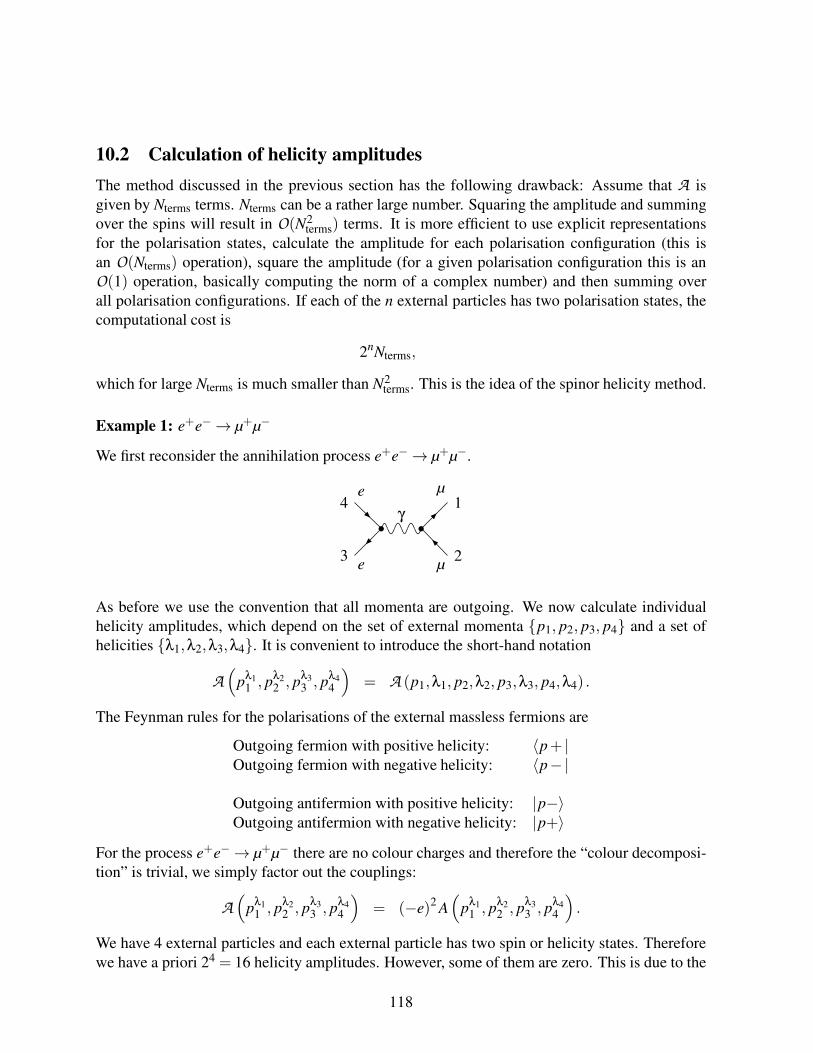
10.2 Calculation of helicity amplitudes
The method discussed in the previous section has the following drawback: Assume that A is
given by Nterms terms. Nterms can be a rather large number. Squaring the amplitude and summing
over the spins will result in O(N2terms) terms. It is more efficient to use explicit representations
for the polarisation states, calculate the amplitude for each polarisation configuration (this is
an O(Nterms) operation), square the amplitude (for a given polarisation configuration this is an
O(1) operation, basically computing the norm of a complex number) and then summing over
all polarisation configurations. If each of the n external particles has two polarisation states, the
computational cost is
2nNterms,
which for large Nterms is much smaller than N2terms. This is the idea of the spinor helicity method.
Example 1: e+e−→ µ+µ−
We first reconsider the annihilation process e+e−→ µ+µ−.
1
23
4µ
µe
e
γ
As before we use the convention that all momenta are outgoing. We now calculate individual
helicity amplitudes, which depend on the set of external momenta p1, p2, p3, p4 and a set of
helicities λ1,λ2,λ3,λ4. It is convenient to introduce the short-hand notation
A(
pλ11 , p
λ22 , p
λ3
3 , pλ44
)
= A (p1,λ1, p2,λ2, p3,λ3, p4,λ4) .
The Feynman rules for the polarisations of the external massless fermions are
Outgoing fermion with positive helicity: 〈p+ |Outgoing fermion with negative helicity: 〈p−|
Outgoing antifermion with positive helicity: |p−〉Outgoing antifermion with negative helicity: |p+〉
For the process e+e−→ µ+µ− there are no colour charges and therefore the “colour decomposi-
tion” is trivial, we simply factor out the couplings:
A(
pλ1
1 , pλ2
2 , pλ3
3 , pλ4
4
)
= (−e)2A(
pλ1
1 , pλ2
2 , pλ3
3 , pλ4
4
)
.
We have 4 external particles and each external particle has two spin or helicity states. Therefore
we have a priori 24 = 16 helicity amplitudes. However, some of them are zero. This is due to the
118
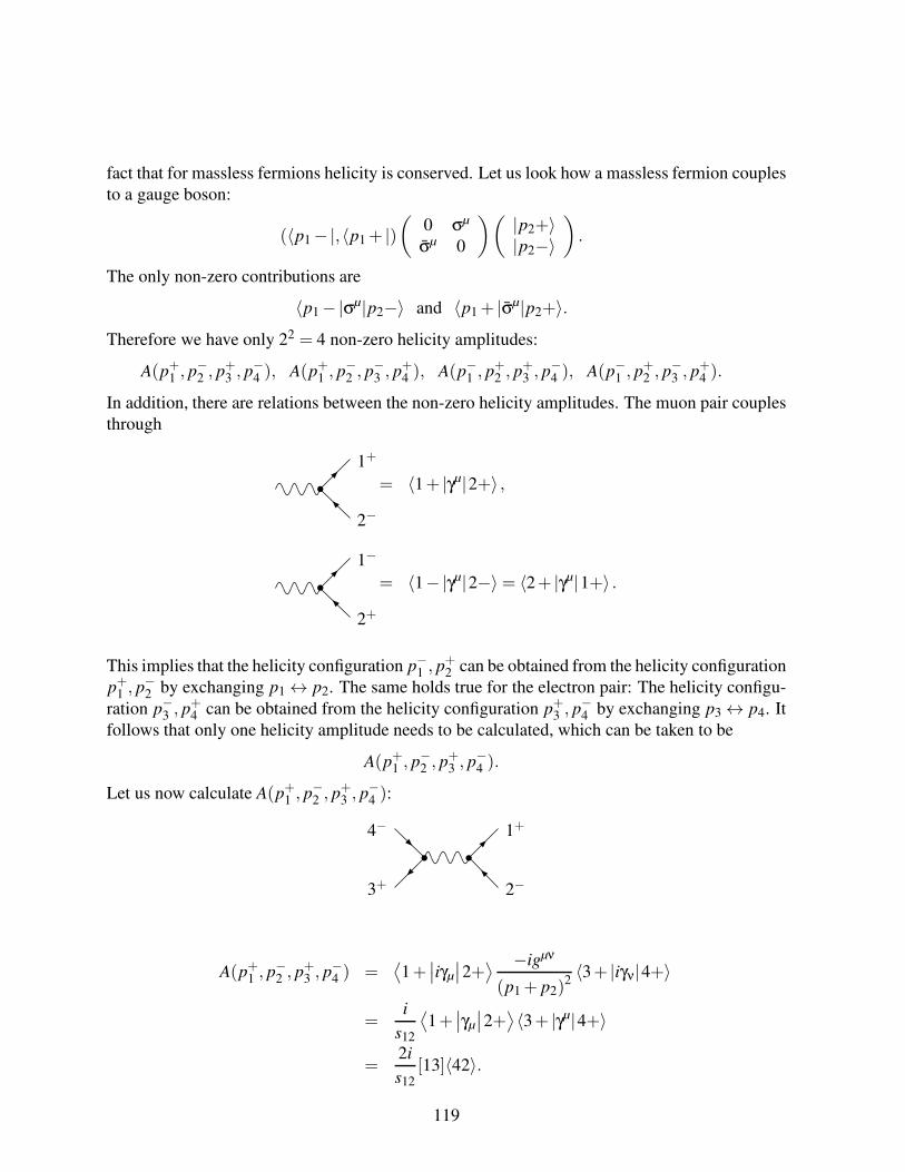
fact that for massless fermions helicity is conserved. Let us look how a massless fermion couples
to a gauge boson:
(〈p1−|,〈p1 + |)(
0 σµ
σµ 0
)(|p2+〉|p2−〉
)
.
The only non-zero contributions are
〈p1−|σµ|p2−〉 and 〈p1 + |σµ|p2+〉.Therefore we have only 22 = 4 non-zero helicity amplitudes:
A(p+1 , p−2 , p+3 , p−4 ), A(p+1 , p−2 , p−3 , p+4 ), A(p−1 , p+2 , p+3 , p−4 ), A(p−1 , p+2 , p−3 , p+4 ).
In addition, there are relations between the non-zero helicity amplitudes. The muon pair couples
through
1+
2−
= 〈1+ |γµ|2+〉 ,
1−
2+
= 〈1−|γµ|2−〉= 〈2+ |γµ|1+〉 .
This implies that the helicity configuration p−1 , p+2 can be obtained from the helicity configuration
p+1 , p−2 by exchanging p1↔ p2. The same holds true for the electron pair: The helicity configu-
ration p−3 , p+4 can be obtained from the helicity configuration p+3 , p−4 by exchanging p3↔ p4. It
follows that only one helicity amplitude needs to be calculated, which can be taken to be
A(p+1 , p−2 , p+3 , p−4 ).
Let us now calculate A(p+1 , p−2 , p+3 , p−4 ):
1+
2−3+
4−
A(p+1 , p−2 , p+3 , p−4 ) =⟨1+∣∣iγµ
∣∣2+
⟩ −igµν
(p1 + p2)2〈3+ |iγν|4+〉
=i
s12
⟨1+∣∣γµ
∣∣2+
⟩〈3+ |γµ|4+〉
=2i
s12[13]〈42〉.
119
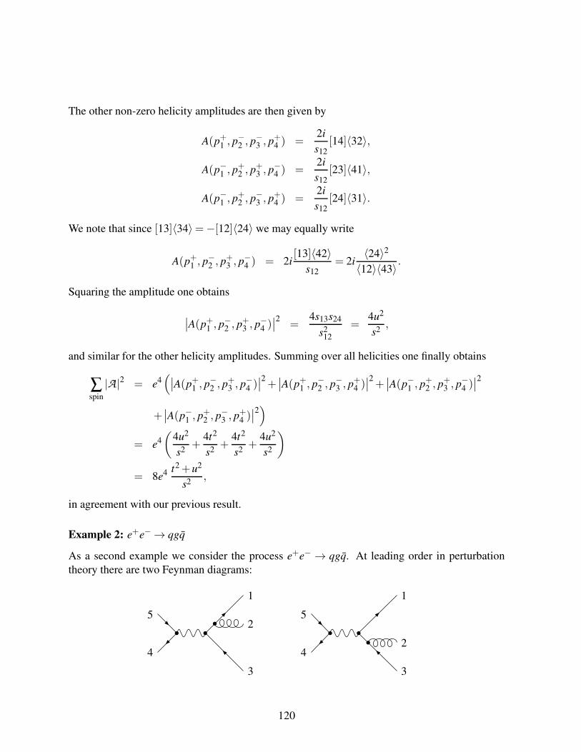
The other non-zero helicity amplitudes are then given by
A(p+1 , p−2 , p−3 , p+4 ) =2i
s12[14]〈32〉,
A(p−1 , p+2 , p+3 , p−4 ) =2i
s12[23]〈41〉,
A(p−1 , p+2 , p−3 , p+4 ) =2i
s12[24]〈31〉.
We note that since [13]〈34〉=−[12]〈24〉 we may equally write
A(p+1 , p−2 , p+3 , p−4 ) = 2i[13]〈42〉
s12= 2i
〈24〉2〈12〉〈43〉 .
Squaring the amplitude one obtains
∣∣A(p+1 , p−2 , p+3 , p−4 )
∣∣2 =
4s13s24
s212
=4u2
s2,
and similar for the other helicity amplitudes. Summing over all helicities one finally obtains
∑spin
|A |2 = e4(∣∣A(p+1 , p−2 , p+3 , p−4 )
∣∣2 +
∣∣A(p+1 , p−2 , p−3 , p+4 )
∣∣2 +
∣∣A(p−1 , p+2 , p+3 , p−4 )
∣∣2
+∣∣A(p−1 , p+2 , p−3 , p+4 )
∣∣2)
= e4
(4u2
s2+
4t2
s2+
4t2
s2+
4u2
s2
)
= 8e4 t2 +u2
s2,
in agreement with our previous result.
Example 2: e+e−→ qgq
As a second example we consider the process e+e− → qgq. At leading order in perturbation
theory there are two Feynman diagrams:
1
2
3
4
5
1
2
3
4
5
120
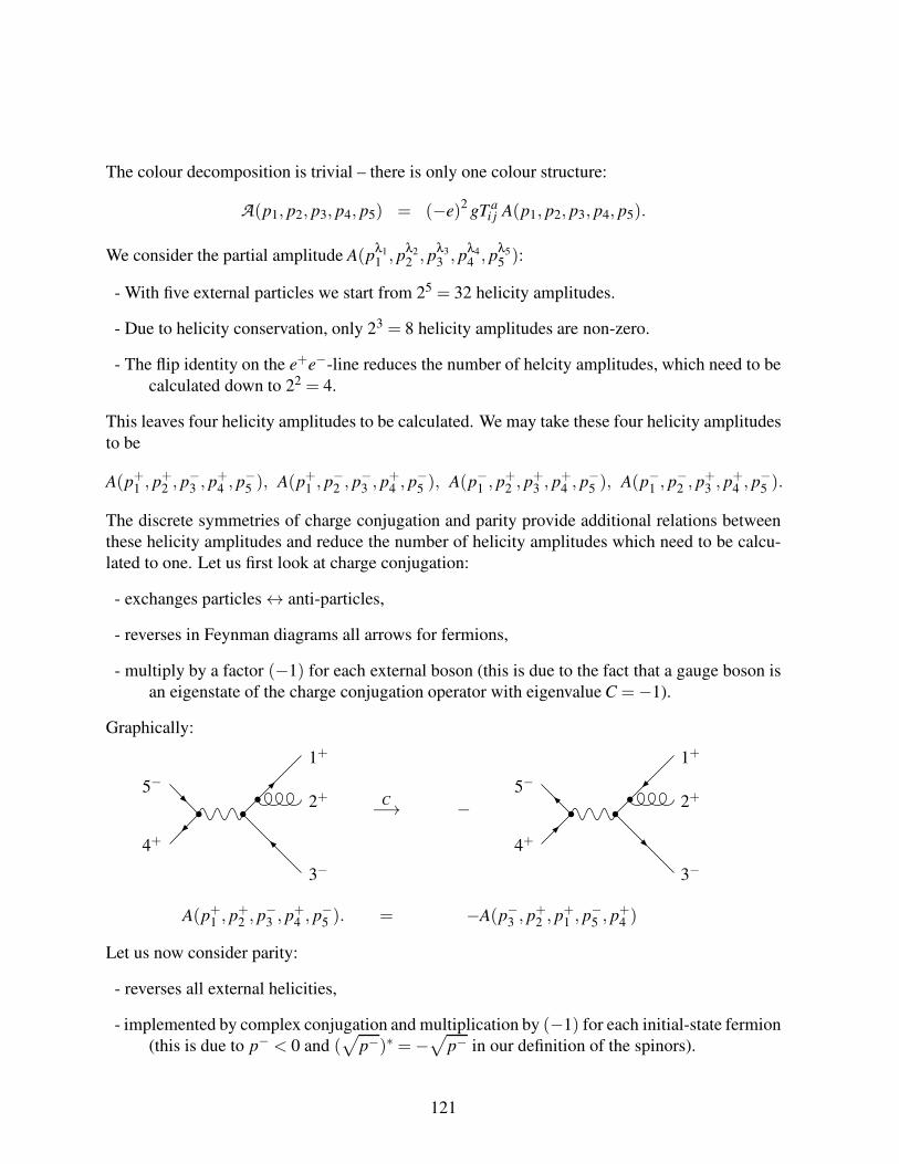
The colour decomposition is trivial – there is only one colour structure:
A(p1, p2, p3, p4, p5) = (−e)2gT a
i j A(p1, p2, p3, p4, p5).
We consider the partial amplitude A(pλ1
1 , pλ2
2 , pλ3
3 , pλ4
4 , pλ5
5 ):
- With five external particles we start from 25 = 32 helicity amplitudes.
- Due to helicity conservation, only 23 = 8 helicity amplitudes are non-zero.
- The flip identity on the e+e−-line reduces the number of helcity amplitudes, which need to be
calculated down to 22 = 4.
This leaves four helicity amplitudes to be calculated. We may take these four helicity amplitudes
to be
A(p+1 , p+2 , p−3 , p+4 , p−5 ), A(p+1 , p−2 , p−3 , p+4 , p−5 ), A(p−1 , p+2 , p+3 , p+4 , p−5 ), A(p−1 , p−2 , p+3 , p+4 , p−5 ).
The discrete symmetries of charge conjugation and parity provide additional relations between
these helicity amplitudes and reduce the number of helicity amplitudes which need to be calcu-
lated to one. Let us first look at charge conjugation:
- exchanges particles↔ anti-particles,
- reverses in Feynman diagrams all arrows for fermions,
- multiply by a factor (−1) for each external boson (this is due to the fact that a gauge boson is
an eigenstate of the charge conjugation operator with eigenvalue C =−1).
Graphically:
1+
2+
3−4+
5−C−→ −
1+
2+
3−4+
5−
A(p+1 , p+2 , p−3 , p+4 , p−5 ). = −A(p−3 , p+2 , p+1 , p−5 , p+4 )
Let us now consider parity:
- reverses all external helicities,
- implemented by complex conjugation and multiplication by (−1) for each initial-state fermion
(this is due to p− < 0 and (√
p−)∗ =−√
p− in our definition of the spinors).
121

Graphically:
1+
2+
3−4+
5−P−→
1−
2−
3+
4−
5+
A(p+1 , p+2 , p−3 , p+4 , p−5 ) = A(p−1 , p−2 , p+3 , p−4 , p+5 )∗.
Therefore only one helicity amplitude needs to be calculated, we may take this helicity amplitude
to be A(p+1 , p+2 , p−3 , p+4 , p−5 ). The two Feynman diagrams are
1+
2+
3−4+
5−1+
2+
3−4+
5−
For the polarisation vector of the gluon we use
ε+µ (p2,q) =
⟨q−∣∣γµ
∣∣ p2−
⟩
√2〈qp2〉
.
Let us choose q = p3: Part of second diagram yields
2+
3−...γµ |3+〉
⟨3−∣∣γµ
∣∣2−
⟩
√2〈32〉
= ... |2−〉√
2
〈32〉 〈3−|3+〉︸ ︷︷ ︸
0
.
Therefore we need to calculate for this choice of reference momentum only the first diagram:
1+
2+,q = p3
3−4+
5−
122
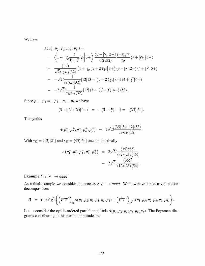
We have
A(p+1 , p+2 , p−3 , p+4 , p−5 ) =
=
⟨
1+
∣∣∣∣iγµ
i
1/+2/iγν
∣∣∣∣3+
⟩ ⟨3−∣∣γµ
∣∣2−
⟩
√2〈32〉
(−i)gνρ
s45
⟨4+∣∣iγρ
∣∣5+
⟩
=(−i)√
2s12s45〈32〉⟨1+∣∣γµ (1/+2/)γν
∣∣3+
⟩〈3−|γµ|2−〉〈4+ |γν|5+〉
= −√
2i1
s12s45〈32〉 [12]〈3−|(1/+2/)γν|3+〉〈4+ |γν|5+〉
= −2√
2i1
s12s45〈32〉 [12]〈3−|(1/+2/)|4−〉〈53〉.
Since p1 + p2 =−p3− p4− p5 we have
〈3−|(1/+2/)|4−〉 = −〈3−|5/|4−〉=−〈35〉[54].
This yields
A(p+1 , p+2 , p−3 , p+4 , p−5 ) = 2√
2i〈35〉[54][12]〈53〉
s12s45〈32〉 .
With s12 = 〈12〉[21] and s45 = 〈45〉[54] one obtains finally
A(p+1 , p+2 , p−3 , p−4 , p+5 ) = 2√
2i〈35〉〈53〉〈32〉〈21〉〈45〉
= 2√
2i〈35〉2
〈12〉〈23〉〈54〉.
Example 3: e+e−→ qggq
As a final example we consider the process e+e− → qggq. We now have a non-trivial colour
decomposition:
A = (−e)2g2
(
T aT b)
i jA(p1, p2, p3, p4, p5, p6)+
(
T bT a)
i jA(p1, p3, p2, p4, p5, p6)
.
Let us consider the cyclic-ordered partial amplitude A(p1, p2, p3, p4, p5, p6). The Feynman dia-
grams contributing to this partial amplitude are:
123
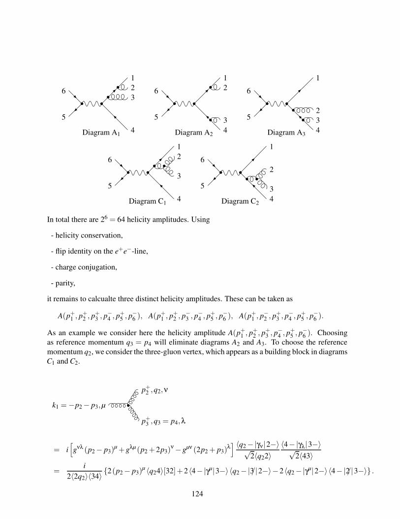
Diagram A1
1
2
3
4
5
6
Diagram A2
1
2
3
4
5
6
Diagram A3
1
2
3
4
5
6
Diagram C1
1
2
3
4
5
6
Diagram C2
1
2
3
4
5
6
In total there are 26 = 64 helicity amplitudes. Using
- helicity conservation,
- flip identity on the e+e−-line,
- charge conjugation,
- parity,
it remains to calcualte three distinct helicity amplitudes. These can be taken as
A(p+1 , p+2 , p+3 , p−4 , p+5 , p−6 ), A(p+1 , p+2 , p−3 , p−4 , p+5 , p−6 ), A(p+1 , p−2 , p+3 , p−4 , p+5 , p−6 ).
As an example we consider here the helicity amplitude A(p+1 , p+2 , p+3 , p−4 , p+5 , p−6 ). Choosing
as reference momentum q3 = p4 will eliminate diagrams A2 and A3. To choose the reference
momentum q2, we consider the three-gluon vertex, which appears as a building block in diagrams
C1 and C2.
p+2 ,q2,ν
p+3 ,q3 = p4,λ
k1 =−p2− p3,µ
= i[
gνλ (p2− p3)µ +gλµ (p2 +2p3)
ν−gµν (2p2 + p3)λ] 〈q2−|γν|2−〉√
2〈q22〉〈4−|γλ|3−〉√
2〈43〉
=i
2〈2q2〉〈34〉 2(p2− p3)µ 〈q24〉[32]+2〈4−|γµ|3−〉〈q2−|3/|2−〉−2〈q2−|γµ|2−〉〈4−|2/|3−〉 .
124
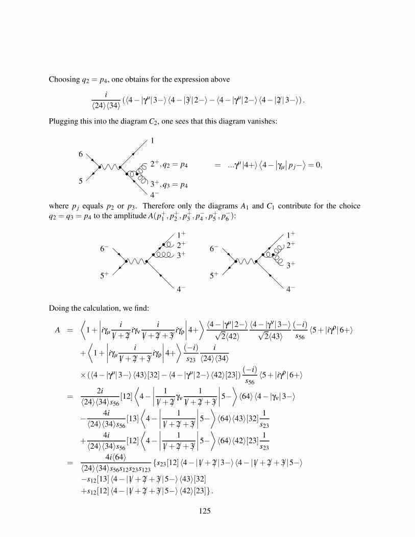
Choosing q2 = p4, one obtains for the expression above
i
〈24〉〈34〉 (〈4−|γµ|3−〉〈4−|3/|2−〉−〈4−|γµ|2−〉〈4−|2/|3−〉) .
Plugging this into the diagram C2, one sees that this diagram vanishes:
1
2+,q2 = p4
3+,q3 = p4
4−5
6
= ...γµ |4+〉⟨4−∣∣γµ
∣∣ p j−
⟩= 0,
where p j equals p2 or p3. Therefore only the diagrams A1 and C1 contribute for the choice
q2 = q3 = p4 to the amplitude A(p+1 , p+2 , p+3 , p−4 , p+5 , p−6 ):
1+
2+
3+
4−5+
6−1+
2+
3+
4−5+
6−
Doing the calculation, we find:
A =
⟨
1+
∣∣∣∣iγµ
i
1/+2/iγν
i
1/+2/+3/iγρ
∣∣∣∣4+
⟩ 〈4−|γµ|2−〉√2〈42〉
〈4−|γν|3−〉√2〈43〉
(−i)
s56〈5+ |iγρ|6+〉
+
⟨
1+
∣∣∣∣iγµ
i
1/+2/+3/iγρ
∣∣∣∣4+
⟩(−i)
s23
i
〈24〉〈34〉
×(〈4−|γµ|3−〉〈43〉[32]−〈4−|γµ|2−〉〈42〉[23])(−i)
s56〈5+ |iγρ|6+〉
=2i
〈24〉〈34〉s56
[12]
⟨
4−∣∣∣∣
1
1/+2/γν
1
1/+2/+3/
∣∣∣∣5−⟩
〈64〉〈4−|γν|3−〉
− 4i
〈24〉〈34〉s56[13]
⟨
4−∣∣∣∣
1
1/+2/+3/
∣∣∣∣5−⟩
〈64〉〈43〉[32]1
s23
+4i
〈24〉〈34〉s56[12]
⟨
4−∣∣∣∣
1
1/+2/+3/
∣∣∣∣5−⟩
〈64〉〈42〉[23]1
s23
=4i〈64〉
〈24〉〈34〉s56s12s23s123s23[12]〈4−|1/+2/|3−〉〈4−|1/+2/+3/|5−〉
−s12[13]〈4−|1/+2/+3/|5−〉〈43〉[32]
+s12[12]〈4−|1/+2/+3/|5−〉〈42〉[23] .
125
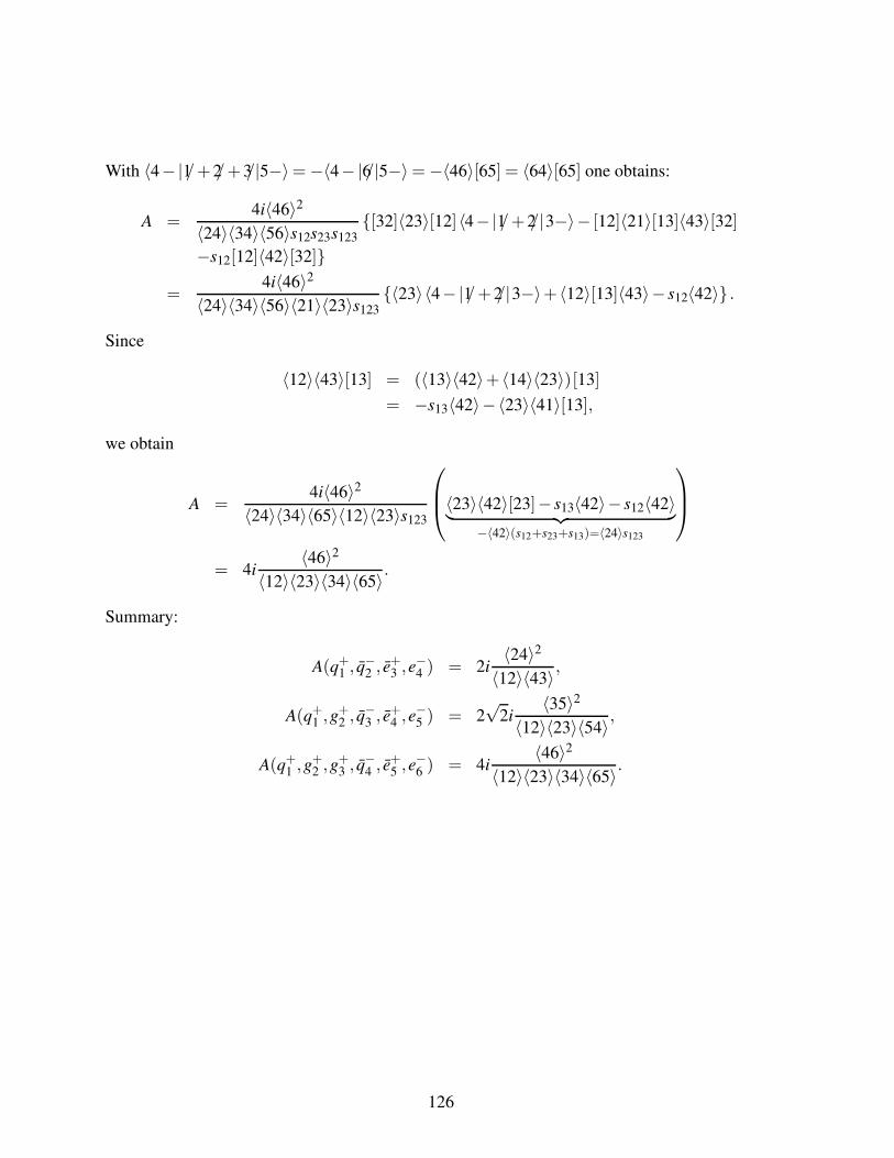
With 〈4−|1/+2/+3/|5−〉=−〈4−|6/|5−〉=−〈46〉[65] = 〈64〉[65] one obtains:
A =4i〈46〉2
〈24〉〈34〉〈56〉s12s23s123[32]〈23〉[12]〈4−|1/+2/|3−〉− [12]〈21〉[13]〈43〉[32]
−s12[12]〈42〉[32]
=4i〈46〉2
〈24〉〈34〉〈56〉〈21〉〈23〉s123〈23〉〈4−|1/+2/|3−〉+ 〈12〉[13]〈43〉− s12〈42〉 .
Since
〈12〉〈43〉[13] = (〈13〉〈42〉+ 〈14〉〈23〉)[13]
= −s13〈42〉−〈23〉〈41〉[13],
we obtain
A =4i〈46〉2
〈24〉〈34〉〈65〉〈12〉〈23〉s123
〈23〉〈42〉[23]− s13〈42〉− s12〈42〉︸ ︷︷ ︸
−〈42〉(s12+s23+s13)=〈24〉s123
= 4i〈46〉2
〈12〉〈23〉〈34〉〈65〉.
Summary:
A(q+1 , q−2 , e
+3 ,e−4 ) = 2i
〈24〉2〈12〉〈43〉,
A(q+1 ,g+2 , q
−3 , e
+4 ,e−5 ) = 2
√2i
〈35〉2〈12〉〈23〉〈54〉,
A(q+1 ,g+2 ,g
+3 , q
−4 , e
+5 ,e−6 ) = 4i
〈46〉2〈12〉〈23〉〈34〉〈65〉.
126