1

TOP OF THE CLASS: THE IMPORTANCE OF

ORDINAL RANK

Richard Murphy† and Felix Weinhardt* *

This version: 1/11/2014

This paper examines the long-run impact of ordinal rank during

primary school on productivity using comprehensive English

administrative data. Identification is obtained from variation in test

score distributions across cohorts and subjects, such that the same

score relative to the school mean can have different ranks.

Conditional on cardinal measures of achievement, being ranked

highly during primary school has large effects on secondary school

achievement, with the impact of rank being more important for boys

than girls. Using additional survey data we find that the

development of confidence is the most likely mechanisms for this

effect on task-specific productivity.

Keywords: rank, non-cognitive skills, peer effects, productivity

JEL: I21, J24

We thank Johannes Abeler, Esteban Aucejo, Thomas Breda, Andrew Clark, Susan Dynarski, Ben Faber, Eric

Hanushek, Brian Jacob, Pat Kline, Steve Machin, Magne Mogstad, Imran Rasul, Olmo Silva, Kenneth Wolpin,

Gill Wyness, and participants of the CEP Labour Market Workshop, the Sussex University, Queen Mary University

and Royal Holloway-University departmental seminars, the CMPO seminar group, the RES Annual Conference

panel, IWAEE, the Trondheim Educational Governance Conference, the SOLE conference, CEP Annual

Conference, the UCL PhD Seminar, the BeNA Berlin Seminar, IFS seminar and the CEE Education Group for

valuable feedback and comments. Weinhardt acknowledges ESRC funding (ES/J003867/1). All remaining errors

are our own.

† University of Texas at Austin, Centre for Economic Performance (CEP). richard.murphy@ucl.ac.uk

* Humboldt-University Berlin, DIW, Centre for Economic Performance (CEP) and IZA.

felix.weinhardt@hu-berlin.de

2

1 Introduction

It is human nature to make comparisons against one’s peers. Individuals make comparisons in

terms of characteristics, traits and abilities (Festinger, 1954). However, individuals also often

use cognitive shortcuts to simplify decision-making (Tversky and Kahneman, 1974). One such

shortcut would be to use simple ordinal rank information instead of detailed cardinal

information. Rather than working out where one stands in relation to the group mean, one

might say ‘I am taller than Gill but shorter than Sarah’. In this simplified way of

conceptualising the world, when making decisions one would be placing weight on ordinal

rank as well as relative or absolute information. Indeed, it has recently been shown that ordinal

rank, in addition to relative position, is used when individuals make comparisons with others

(Brown et al., 2008; Card et al., 2012). If people are ranking themselves amongst their peers,

then ordinal in additional to cardinal information has the potential to affect investment

decisions, which in turn could in in turn determine later productivity.

This paper examines, in the context of education, the additional impact of ordinal rank on

subsequent productivity. We use five cohorts of the English student population on their

transition from primary school age 11 to secondary school age 14.1 Students in England take

externally marked national exams at the end of primary school, which we use to calculate their

rank amongst their peers in three subjects. These students then start attending secondary

schools with a new set of peers and are tested again in the same subjects three years later.

Therefore we estimate the effect of prior rank during primary education on age-14 test scores,

three years into a new secondary school peer environment conditional on prior age-11 relative

test scores.

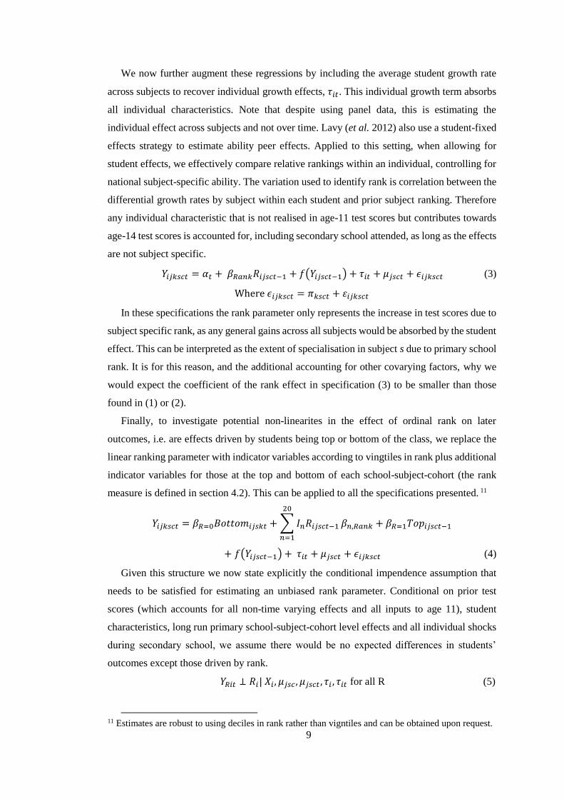
The rank parameter is identified from the variation in test score distributions across and

within primary schools cohorts, so that the same score relative to a school mean can have

different ranks (Figure 1). Our estimates show that being highly ranked amongst your peers

in a subject has large and robust effects on later performance in that same subject. Moreover,

the impact of rank is significant across the entire rank distribution. These estimates use the

school-by-subject-by-cohort variation in rank for a given test score and therefore allow for

gains from individuals being ranked highly in one subject to impact on results on other

subjects. We also provide more demanding within-student specifications, which absorb the

average growth rate of a student between age 11 and 14, thereby removing subject-spillovers

and so reflect student specialisation. In these specifications, the variation used for estimation

is the within-student-across-subject differences in rank conditional on test scores and prior

school environment. We argue that conditioning on these age-11 test scores, primary-subject-

1 Public schools account for 93% of the total student population in England. Comparable data for the

remaining 7% attending private schools are not available.

3

cohort effects and individual student effects, the ranking of a student in a subject within

primary school is effectively random.

Notably, primary school peers determine the rank measure but we estimate its effects on

outcomes after the transition to secondary school. This makes our approach resilient to

reflection problems (Manski, 1993) as the average student has 87% new peers in secondary

school. We are therefore not relating individual and group outcomes from within the same

peer group, as cautioned against by Angrist (2013). Using the transition from the end of

primary school to secondary school relieves concerns about tracking or other inputs based on

rank during the primary phase, as they will be captured in the end-of-primary test scores.

Additionally any shocks, unobserved teacher abilities etc. that give rise to different

distributions during the primary phase, and thus generate variation in ordinal rank conditional

on own and average primary peer achievement, will also be absorbed by these test scores.

While these factors are unobserved to the researcher, they are predetermined from the point

of our analysis, which is at the secondary school level. Furthermore, any secondary school

inputs based on rank are also not a concern as students with the same test scores in primary

school would expect to have the same rank when entering secondary school. As a result, we

identify the rank parameter as long as children do not sort into schools according to rank

conditional on ability, which we observe to be the case. In addition, our estimation sidesteps

the standard issue of including a lagged dependent variable and individual effects

simultaneously (Nickell, 1981), as the individual effects are recovered from the average

growth in test scores across subjects, rather than from average test scores over time.

The effects of rank that we present are sizable in the context of the education literature,

with a one standard deviation increase in rank improving age-14 test scores by 0.08 standard

deviations. This is of comparable magnitude to being taught by a teacher one standard

deviation above average (Aaronson, et al., 2007; Hanushek et al., 2005). As expected, the

estimates relying on within-student variation in primary rank, conditional on ability, are

smaller. Here, a one standard deviation increase in rank improves subsequent test scores in

that subject by 0.055 within student standard deviations. This would mean being ranked at the

75th percentile of your primary school peers in a subject as opposed to the 25th percentile,

improves age 14 test scores by 0.2 standard deviations in that same subject.

The paper goes on to examine the nature of these effects and finds that they exist

throughout the rank distribution, implying that students can accurately place themselves

within their class, despite not being explicitly informed of their rank. Ultimately the

mechanism must involve students’ perceived ranking, however there are no large

administrative datasets that contain such information. Therefore, we instead use an objective

measure of an individual’s actual rank in a task as a close substitute, given their highly

4

correlated nature.2 This can be thought of as the reduced form, in place of perceived rank, and

to the extent that the first stage is weak, we will be obtaining an underestimate of the true

impact of rank. This is likely to occur due to the repeated interactions among peers throughout

the six years of primary school as well as seating arrangements that that reflect rank positions

in many English primary schools.3 Moreover, for nearly all rank positions boys are more

affected, both positively and negatively, than girls. Boys at the top of the class in a subject

gain four times more than comparable girls. Low-income students also gain more from being

top of the class but are less negatively affected by being ranked below the median. Having

presented this range of findings, the paper examines and tests threats to identification such as

other forms of peer effects, measurement error and sorting to schools by parents.

Finally the paper considers and rules out a number of mechanisms that could account for

these results: competitiveness; external investment by task; environment favouring certain

ranks; and learning about ability (Ertac, 2006). We propose that the mechanism that best

accommodate all the findings is that being highly ranked in a task improves associated non-

cognitive skills such as confidence, which reduces the cost of effort for that task. One might

consider one’s own school career. Upon starting school, we may not know which subjects we

are good at. But, through comparing our standing relative to our peers by the end of primary

school we develop a sense that we are a ‘math person’ or a ‘language person’. A ‘math person’

would be more confident in solving mathematical problems and enjoy math more, and so

during secondary may invest more effort into math homework, all of which could be reflected

in their future math test scores.

Through combining our administrative data with survey data containing direct measures

of subject-specific confidence, we show that those who ranked higher in primary school have

larger measures of later confidence, conditional on relative test scores and student effects.

Mirroring our findings on attainment, we find that boys’ confidence is more affected by their

school rank than girls’ confidence.

To build intuition for the effect of confidence and the generalizability of the results,

consider a good lawyer at the top law firm. Despite being competent, they are surrounded by

the best and so are lowly ranked. This would lower their confidence in being a lawyer and so

2 The ability to rank yourself within a group is a long standing topic in the psychological literature

(Beyer 1990, Littlepage, Robison, & Reddington, 1997). The have found that accuracy is greatly

improved where there is prolonged face to face interactions (Kenny, 1991, Paulhus & Bruce, 1992),

when the task is well defined (as opposed to ranks in ‘friendliness or ‘leadership’) and when the action

has already occurred (as opposed to predicting future rankings) (Jourden and Heath, 1996). All of these

factors conducive to correct ranking are present amongst primary school students who spend six years

in the same classroom as each other. 3 In English Primary schools it is common for students to be seated at tables of four and for them to be

set by pupil ability. Students can be sat at the ‘top table’ or the ‘bottom/naughty table’. This could assist

students in establishing where they rank amongst all class members through a form of batch algorithm,

e.g. ‘I’m on top table, but I’m the worst, therefore I’m fourth best.’

5

may change career. Whereas, if the lawyer had joined a less prestigious firm, they would have

been more highly ranked and gained in confidence. This would lead to lowing the cost of

effort and so would invest more time in work, becoming more skilled, and eventually

becoming a partner.

We believe this paper has two main contributions. First, to the best of the authors’

knowledge this is the first large-scale study to document the effects of ordinal rank in a task

on later productivity. Critically, this study documents an additional effect of ordinal rank, after

controlling for prior achievement and the relative distances between peers, i.e. cardinal

measures of performance. Therefore, we believe perceived rank could be considered a new

factor in the education production function.4 Besides implications on partial equilibrium

considerations of parents regarding the choice of the best school for their children, this finding

has more general implications relating to informational transparency and productivity. For

instance managers or teachers could improve productivity by emphasising an individual’s

local rank position if that individual has a high rank. Alternatively, if an individual is in a high

performing peer group and therefore may have a low local rank but ranks high globally, a

manager should make the global rank more salient.

Secondly, we believe that the result that perceived ordinal rank matters for later outcomes

has the potential to add to the explanation of findings in the following education topics where

placing individuals amongst high-performing peers has had mixed results: school integration

(Angrist and Lang, 2004; Kling et al. 2007) selective schools (Cullen et al. 2006; Clark 2010);

and affirmative action (Arcidiacono et al. 2012; Robles and Krishna, 2012). Moreover the

finding that rank may exacerbate early differences in achievement due to individual

investment decisions based on relative performance contributes to the literatures on ethnicity

(Fryer and Levitt, 2006; Hanushek and Rivkin 2006; 2009), gender (Burgess et al, 2004;

Machin & McNally, 2005) and relative age in cohort (i.e. Black et al., 2011).

The remainder of the paper is laid out as follows. Section 2 reviews the literature on social

comparisons. Section 3 sets out the empirical strategy and how the rank parameter is separately

identified from relative achievement. This is followed by a brief description of the UK

educational system, the administrative data, as well as the definition of rank used. Section 5

sets out the main results, nonlinearities and the heterogeneity by gender and parental income.

Section 6 discusses and tests threats to identification such as peer effects, measurement error

and endogenous sorting. Section 7 discusses potential mechanisms and provides additional

4 There is a broad range of literature on the determinants of academic achievements, including natural

ability (Watkins et al., 2007), family background (Hoxby, 2001), school inputs (Hanushek, 2006; Page

et al., 2010), peer effects (Carrell et al., 2009; Lavy et al., 2012), and non-cognitive skills (Heckman et

al., 2006); however, rank position has not yet been researched.

6

survey evidence. Finally, in Section 8 we conclude by discussing other topics in education

which corroborate these findings and possible policy implications.

2 Related Literature

The importance of ordinal rank rather than relative position for individuals was first

forwarded by Parducci (1965) with range frequency theory. This has the theoretical prediction

that comparisons are based upon ordinal position of items within a comparison set. This

prediction has been illustrated empirically recently by Brown et al. (2008) and Card et al.

(2012), who show an individual’s rank in addition to relative position in an income distribution

is an important determinant of satisfaction. However, the economic literature on rank effects

on productivity is sparse.5

A related study on rank and informational transparency finds that providing employees

with their productivity rank within the firm increased output throughout the productivity

distribution (Blanes i Vidal and Nossol 2011). This is explained by workers becoming

concerned about their rank position, as the impact occurred after the feedback policy was

announced but before the information was released.6 Genakos and Pagliero (2012) find that in

a tournament setting, where payoffs are based on relative performance and with continuous

rank feedback, performance decreases as individuals are ranked higher.7 In both of these

papers, individuals are concerned about their relative positions amongst their immediate peers.

The education setting of this study varies in two critical ways. Firstly, students are graded on

their absolute performance according to national scales, rather than relative to their peers.

Secondly, we are estimating the effect of rank amongst previous peers on contemporaneous

test scores, and not the effects of rank within the same peer group. Moreover, whilst both of

these papers use rank measurements, neither additionally controls for relative distances, and

are therefore not separating rank effects from any cardinal relative effects.

The paper most closely related to ours is by Clark et al. (2010), who compare directly the

importance of ordinal rather than relative position on discretionary work effort. They find that

an employee’s income rank was a stronger determinant of stated work effort compared with

5 The discussion of social comparisons is often framed in the form of peer effects (Falk and Ichino,

2006; Mas and Moretti, 2009, Carrell et al., 2009; Lavy et al., 2012) or the introduction of relative

achievement feedback mechanisms (Eriksson et al. 2009; Azmat and Iriberri, 2010). These studies tend

to find positive effects of peer quality on contemporaneous productivity, and that relative performance

feedback increases productivity when there are piece rate incentives. 6 Kosfeld and Neckerman (2011) examine the use of rankings as a non-monetary incentive and find

increases in productivity. Specific to education, Jalava, Joensen and Pellas (2013) find that rank based

grading increases test performance. 7 Brown (2011) shows in a tournament setting that when an individual of known outstanding ability

(high prior high rank is known) is placed into a group those ranked immediately below them, have a

large fall in productivity compared to low ranked participants.

7

the average reference group income and so conclude that comparisons are ordinal rather than

cardinal. This is similar to our paper as we also in effect estimate effects of rank and relative

position, but differ as we observe rank effects in a real effort setting rather than in stated

amounts and estimate the impact in a different peer setting.

3 Empirical strategy

3.1 A rank-augmented education production function

We use the standard education production function approach to derive a rank-augmented

value added specification that can be used to identify the effect of primary school rank,

measured as outlined in section 4.2 Error! Reference source not found., on subsequent

outcomes.8

We use the education function framework set out in Todd and Wolpin (2003), for student

i studying subject s in secondary school k, from primary school j, cohort c and in time period

𝑡 = [0,1]. Our basic specification is the following:

𝑌𝑖𝑗𝑘𝑠𝑐𝑡 = 𝛽𝑅𝑎𝑛𝑘𝑅𝑖𝑗𝑠𝑐𝑡−1 + 𝑓(𝑌𝑖𝑗𝑠𝑐𝑡−1) + 𝑋𝑖′𝛽𝑡 + 𝜇𝑗𝑠𝑐𝑡 + 𝜖𝑖𝑗𝑘𝑠𝑐𝑡 (1)

Where 𝜖𝑖𝑗𝑘𝑠𝑐𝑡 = 𝜏𝑖𝑡 + 𝜋𝑘𝑠𝑐𝑡 + 휀𝑖𝑗𝑘𝑠𝑐𝑡

where Y denotes national academic percentile rank in subject s at time t. In this setting we

only have two time periods, with the initial (t-1) representing primary school and next (t)

representing secondary school and three subjects. Student achievement is determined by a

series observable and unobservable characteristics and shocks. Conditioning on end of

primary school test schools, captures all factors up to the end of primary school such as student

ability, parental investment, or school inputs. In our regressions, we will allow the functional

form of this lagged dependent variable to take two forms, either a 3rd degree polynomial or a

fully flexible measure, which allows for a different effect at each national test score percentile

We allow for students growth in attainment to vary from age 11 to 14 according to X a

vector of observable permanent characteristics of the student. Moreover, we allow for the

primary school to have longer run impacts on student achievement not captured by the end of

school test scores, by including by primary school-subject-cohort effects, 𝜇𝑗𝑠𝑐𝑡. This could

reflect that a school is very good at increasing the efficiency of their students to learn maths

in the future in one cohort, and for English in the next cohort. Note that with the inclusion of

primary-subject-cohort effects, the test score then becomes a measure of relative cardinal

ability to the cohort. The parameter of interest is 𝛽𝑅𝑎𝑛𝑘, which is the effect of having rank

𝑅𝑖𝑗𝑠𝑐 𝑡−1, in subject s in cohort c and in primary school j on student achievement in that subject

8 To see a full derivation from a more basic model see Appendix 3

8

during secondary school.9 Rank is measured by a student’s percentile rank in a subject in their

school cohort, and can take values from 0 to 1 inclusive, further details are presented in the

data section.

The remaining unobservable factor 𝜖𝑖𝑗𝑘𝑠𝑐𝑡 , is formed of three components; unobserved

individual specific second period shocks 𝜏𝑖𝑡; the overall impact of attending secondary school

k on subject s in cohort c 𝜋𝑘𝑠𝑐𝑡; and an idiosyncratic error term 휀𝑖𝑗𝑘𝑠𝑐𝑡. The discussion of

recovering 𝜏𝑖𝑡, the academic growth of individual i during secondary school is below, but it is

worth spending some time interpreting what the rank coefficient represents without its

inclusion. Being ranked highly in primary school may have positive spillover effect in other

subjects. Any estimation, which allows for individual growth rates during secondary school

(second period), would absorb any spillover effects. Therefore, leaving 𝜏𝑖 in the residual

means that the rank parameter is the effect of rank of the subject in question and the correlation

in rank between the other two subjects.

Given that not all secondary schools are the same, it is expected that the secondary school

attended will impact on age 14 test scores by subject. This would be a concern to our estimates

of the rank parameter if students selected their secondary schools based on their rank in a

particular subject during primary school in addition to their age-11 test scores. If, for example,

students who were top of their class in maths aspire to attend to a secondary school that

specialises in maths, our estimates could be confounded by secondary school quality. This

might seem unlikely because we know that ability sorting for secondary schools in England is

largely based on average rather than subject-specific abilities (Lavy et al. 2012).

𝑌𝑖𝑗𝑘𝑠𝑐𝑡 = 𝛽𝑅𝑎𝑛𝑘𝑅𝑖𝑗𝑠𝑐𝑡−1 + 𝑓(𝑌𝑖𝑗𝑠𝑐𝑡−1) + 𝑋𝑖′𝛽 + 𝜇𝑗𝑠𝑐𝑡 + 𝜋𝑘𝑠𝑐𝑡 + 𝜓𝑖𝑗𝑘𝑠𝑐𝑡 (2)

Where 𝜓𝑖𝑗𝑘𝑠𝑐𝑡 = 𝜏𝑖𝑡 + 휀𝑖𝑗𝑘𝑠𝑡

Fortunately, our data allows us to address this concern directly by additionally controlling

for secondary school attended. Specification 2 additionally allows for second achievement to

vary by secondary school k in subject s of cohort c, 𝜋𝑘𝑠𝑐𝑡.10 Intuitively, this is comparing

students who are exposed to the same secondary school influences, thus identifying effects net

of any potential subject-rank driven sorting into secondary education. However, secondary

school attended can be argued to be an outcome, and therefore should not be conditioned upon.

Specifications that include these effects are not our preferred model and are only used as an

indication of the extent that secondary school selection has effects on the estimates. As we

will see, this modification does not affect our results.

9 Any positive impact of rank during primary school on student test scores would downward bias our

results as it would be captured in the age 11 test scores. 10 We use the Stata command reg2hdfe for these estimations (Guimaraes and Portugal, 2010).

9

We now further augment these regressions by including the average student growth rate

across subjects to recover individual growth effects, 𝜏𝑖𝑡. This individual growth term absorbs

all individual characteristics. Note that despite using panel data, this is estimating the

individual effect across subjects and not over time. Lavy (et al. 2012) also use a student-fixed

effects strategy to estimate ability peer effects. Applied to this setting, when allowing for

student effects, we effectively compare relative rankings within an individual, controlling for

national subject-specific ability. The variation used to identify rank is correlation between the

differential growth rates by subject within each student and prior subject ranking. Therefore

any individual characteristic that is not realised in age-11 test scores but contributes towards

age-14 test scores is accounted for, including secondary school attended, as long as the effects

are not subject specific.

𝑌𝑖𝑗𝑘𝑠𝑐𝑡 = 𝛼𝑡 + 𝛽𝑅𝑎𝑛𝑘𝑅𝑖𝑗𝑠𝑐𝑡−1 + 𝑓(𝑌𝑖𝑗𝑠𝑐𝑡−1) + 𝜏𝑖𝑡 + 𝜇𝑗𝑠𝑐𝑡 + 𝜖𝑖𝑗𝑘𝑠𝑐𝑡 (3)

Where 𝜖𝑖𝑗𝑘𝑠𝑐𝑡 = 𝜋𝑘𝑠𝑐𝑡 + 휀𝑖𝑗𝑘𝑠𝑐𝑡

In these specifications the rank parameter only represents the increase in test scores due to

subject specific rank, as any general gains across all subjects would be absorbed by the student

effect. This can be interpreted as the extent of specialisation in subject s due to primary school

rank. It is for this reason, and the additional accounting for other covarying factors, why we

would expect the coefficient of the rank effect in specification (3) to be smaller than those

found in (1) or (2).

Finally, to investigate potential non-linearites in the effect of ordinal rank on later

outcomes, i.e. are effects driven by students being top or bottom of the class, we replace the

linear ranking parameter with indicator variables according to vingtiles in rank plus additional

indicator variables for those at the top and bottom of each school-subject-cohort (the rank

measure is defined in section 4.2). This can be applied to all the specifications presented. 11

𝑌𝑖𝑗𝑘𝑠𝑐𝑡 = 𝛽𝑅=0𝐵𝑜𝑡𝑡𝑜𝑚𝑖𝑗𝑠𝑘𝑡 + ∑ 𝐼𝑛𝑅𝑖𝑗𝑠𝑐𝑡−1

20

𝑛=1

𝛽𝑛,𝑅𝑎𝑛𝑘 + 𝛽𝑅=1𝑇𝑜𝑝𝑖𝑗𝑠𝑐𝑡−1

+ 𝑓(𝑌𝑖𝑗𝑠𝑐𝑡−1) + 𝜏𝑖𝑡 + 𝜇𝑗𝑠𝑐𝑡 + 𝜖𝑖𝑗𝑘𝑠𝑐𝑡 (4)

Given this structure we now state explicitly the conditional impendence assumption that

needs to be satisfied for estimating an unbiased rank parameter. Conditional on prior test

scores (which accounts for all non-time varying effects and all inputs to age 11), student

characteristics, long run primary school-subject-cohort level effects and all individual shocks

during secondary school, we assume there would be no expected differences in students’

outcomes except those driven by rank.

𝑌𝑅𝑖𝑡 ⊥ 𝑅𝑖| 𝑋𝑖, 𝜇𝑗𝑠𝑐 , 𝜇𝑗𝑠𝑐𝑡 , 𝜏𝑖 , 𝜏𝑖𝑡 for all R (5)

11 Estimates are robust to using deciles in rank rather than vigntiles and can be obtained upon request.

10

In summary, if students react to ordinal information as well as cardinal informaiton, then

we would expect percived rank in adition to relative achivement to have a signficant effect on

later achievement when estimating these equations. However, we do not have student’s

perceived ranking and instead use the proxy of actual rank. This is what is picked up by the

𝛽𝑅𝑎𝑛𝑘-coefficient. This can be thought of as the reduced form, and to the extent that the first

stage is weak, we will be obtaining an underestimate of the true impact. After the results

section, we will address further threats to identification such as measurement error,

unobserved subject specific factors, and other non-standard peer effects.

4 Institutional setting, data and descriptive statistics

4.1 The English School System

The compulsory education system of England is made up of four Key Stages (KS); at the

end of each stage students are evaluated in national exams. Key Stage Two (KS2) is taught

during primary school between the ages of 7 and 11. The median size of a primary school

cohort and the average primary school class size is 27 students (DFE, 2011). Therefore, when

referring to primary school rank, one could consider this as class rank.12 At the end of the final

year of primary school when the students are aged 11, they take KS2 tests in English, math

and science. These tests are externally graded on a national scale of between 0-100. This

makes it possible to make comparisons in student achievement over time and across schools.

Rather than receiving these raw scores, students are instead given one of five broad

attainment levels. The lowest performing students are awarded Level 1, the top performing

students are awarded Level 5. These levels are broad, which results in them being a coarse

measure, with 85% of students achieve Level 4 or 5. These are non-high stakes exams for

students and are mainly used by the government as a measure of school effectiveness.13 This

means that students do not know their underlying exact test score, which we use to calculate

their local ranks. Rather, students infer their rank position in class through repeated interaction

and comparisons between students along with teacher feedback throughout primary school.

Students then transfer to secondary school, where they start working towards the third Key

Stage (KS3). During this transition the average primary school sends students to six different

secondary schools and secondary schools typically receive students from 16 different primary

12 The maximum class size at Key Stage 1 is 30 students. A parallel set of results has been estimated

using only cohorts of 30 and below, assuming these are single class cohorts. The results are qualitatively

the same and are available from the authors upon request. 13 The students also appear not to gain academically just from achieving a higher level. Regression

discontinuity techniques show no gain for those students who just achieved a higher level. This setting

is ideal for a regression discontinuity techniques as the score needed to reach a level changes by year

and by subject, which would make it particularly hard to game.

11

schools. At secondary school, a typical student has 87% new peers upon arrival. This large re-

mixing of peers is beneficial, as it allows us to estimate the impact of rank form a previous

peer group on subsequent outcomes. Importantly, admission into secondary schools is

generally non-selective and does not depend on end-of-primary KS2 test scores. A subset of

schools can select on ability (grammar schools) but these schools administer their own

admission tests. The KS2 is thus a low-stakes test with respect to secondary school choice,

moreover even if it was used it is likely that admissions would be based on coarse absolute

levels, rather than relative ranking Key Stage 3 takes place over three years and at the end of

Year 9, all students take KS3 examinations in English, math and science at age fourteen. Again

KS3 is not a high-stakes test and is externally marked.14

4.2 Data Construction

4.2.1 Administrative data

The Department for Education (DfE) collects data on all students and all schools in state

education in England. The Pupil Level Annual School Census (PLASC) contains the school

attended and demographic information such as gender, ethnicity, language skills, Special

Educational Needs (SEN), and being Free School Meals Eligible (FSME). The National Pupil

Database (NPD) contains student attainment data throughout their Key Stage progression in

each of the three compulsory subjects. Each student is given a unique identifier so that they

can be linked to schools and followed over time, allowing the government to produce value

added measures and publish school league tables. As the functions of both of these datasets

are at the school level, no class level data is collected.

We have combined these data to create a dataset following the entire population of five

cohorts of English school children. This begins at the age of 10/11 in the final year of Primary

School when students take their Key Stage 2 examinations through to age 13/14 when they

take Key Stage 3 tests. KS2 examinations were taken in the academic years 2000/2001 to

2005/2006 and so it follows that the KS3 examinations took place in 2003/2004 to 2007/8.

From 2009 students were no longer externally assessed, instead teacher assessment was used

to evaluate students at the end of Key Stage 3, hence this is the end point of our analysis.

We imposed a set of restrictions on the data to obtain a balanced panel of students. We use

only students who can be tracked with valid KS2 and KS3 exam information and background

14 Two years later, students take the national Key Stage 4 test at age 16 (KS4), which marks the end

of compulsory education in England. The KS4 is graded from one to eight and students have some

discretion in choosing the subjects they study and at what level. Since KS3 is graded on a fine scale [0-

100], and students are tested in the same compulsory subjects only, we prefer this as the outcome

measure for the purpose of our study. Using KS4 as an outcome produces qualitatively the same, but

quantitatively slight smaller significant results. Available upon request.

12

characteristics, 83% of the population. Secondly, we exclude students who appear to be double

counted (1,060) and whose school identifiers do not match within a year across datasets,

approximately 0.6% of the remaining sample (12,900). Finally, we remove all students who

attended a primary school whose cohort size was smaller than 10, as these small schools are

likely to be atypical in a number of dimensions; this represents 2.8% of students.15 This leaves

us with approximately 454,000 students per cohort, with a final sample of just under 2.3

million student observations, or 6.8 million student-subject observations.

The Key Stage test scores for both levels are percentalized by subject and cohort, so that

each individual has six test scores between 0 and 100 (three KS2 and three KS3). This ensures

that students of the same nationally relative ability have the same national percentile rank, as

a given test score could represent a different ability in different years or subjects. Importantly,

this allows for test score comparisons to be made across subjects and across time, this does

not impinge on our estimation strategy, which relies only on heterogeneous test score

distributions across schools to generate variation in local rank. 16

We rank students in each subject according to their age 11 national test scores within their

primary school by cohort. Similarly to test scores, to have a comparable local rank

measurement across schools of different cohort size we percentalized the rank position of

individual i with the following tranformation:

𝑅𝑖𝑗𝑠𝑐 =𝑛𝑖𝑗𝑠𝑐−1

𝑁𝑗𝑠𝑐−1, 𝑅𝑖𝑗𝑠𝑐 = [0,1] (6)

where Njsc is the cohort size of school j in cohort c of subject s. An individual’s i ordinal

rank position within this set is nijsc,, which is increasing in test score. Rijsc is the standardised

rank of the student. 17 For example, a student who had the second best score from a cohort of

twenty-one students (nijsc=20, Njsc=21) will have Rijsc=0.95. This rank measure will be

approximately uniformly distributed, and bounded between 0 and 1, with the lowest rank

student in each school cohort having R=0. In the case of draws of national percentile rank,

each of the students is given the lower local rank.

Rank is dependent on students own test scores and also the scores of others in their school

cohort. Again consider the students who scored X and Y in cohorts with different test score

15 Estimations using the whole sample are very similar, only varying at the second decimal point.

Contact authors for further results. 16 Estimations using standardised rather than percentalized test scores provide similar estimates to the

first decimal place in linear specification. For non-linear specifications the effect of rank appears more

cubic in nature. However, these estimations suffer from non-comparability as a given test score could

represent a different ability in different years or subjects. Year/subject effects would not account for all

these differences as there are likely to be distributional differences. Allowing for either functional form

of test scores to be interacted by year and subject was extremely computationally intensive, given our

already demanding specification. Basic results are available from the authors upon request. 17 This is rank within school subject cohort, it cannot be done by class as no class level information is

available. However, all estimations have been replicated on schools which have cohort sizes of under

30 (maximum class size) and have equivalent results. Obtainable upon request.

13

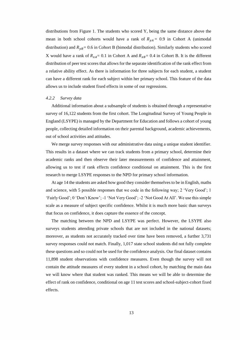
distributions from Figure 1. The students who scored Y, being the same distance above the

mean in both school cohorts would have a rank of 𝑅𝑦𝐴 = 0.9 in Cohort A (unimodal

distribution) and 𝑅𝑦𝐵= 0.6 in Cohort B (bimodal distribution). Similarly students who scored

X would have a rank of 𝑅𝑥𝐴= 0.1 in Cohort A and 𝑅𝑥𝐵= 0.4 in Cohort B. It is the different

distribution of peer test scores that allows for the separate identification of the rank effect from

a relative ability effect. As there is information for three subjects for each student, a student

can have a different rank for each subject within her primary school. This feature of the data

allows us to include student fixed effects in some of our regressions.

4.2.2 Survey data

Additional information about a subsample of students is obtained through a representative

survey of 16,122 students from the first cohort. The Longitudinal Survey of Young People in

England (LSYPE) is managed by the Department for Education and follows a cohort of young

people, collecting detailed information on their parental background, academic achievements,

out of school activities and attitudes.

We merge survey responses with our administrative data using a unique student identifier.

This results in a dataset where we can track students from a primary school, determine their

academic ranks and then observe their later measurements of confidence and attainment,

allowing us to test if rank effects confidence conditional on attainment. This is the first

research to merge LSYPE responses to the NPD for primary school information.

At age 14 the students are asked how good they consider themselves to be in English, maths

and science, with 5 possible responses that we code in the following way; 2 ‘Very Good’; 1

‘Fairly Good’; 0 ‘Don’t Know’; -1 ‘Not Very Good’; -2 ‘Not Good At All’. We use this simple

scale as a measure of subject specific confidence. Whilst it is much more basic than surveys

that focus on confidence, it does capture the essence of the concept.

The matching between the NPD and LSYPE was perfect. However, the LSYPE also

surveys students attending private schools that are not included in the national datasets;

moreover, as students not accurately tracked over time have been removed, a further 3,731

survey responses could not match. Finally, 1,017 state school students did not fully complete

these questions and so could not be used for the confidence analysis. Our final dataset contains

11,898 student observations with confidence measures. Even though the survey will not

contain the attitude measures of every student in a school cohort, by matching the main data

we will know where that student was ranked. This means we will be able to determine the

effect of rank on confidence, conditional on age 11 test scores and school-subject-cohort fixed

effects.

14

4.3 Descriptive statistics

4.3.1 Main sample

The data has the complete coverage of the state student population from age 10 to 14. We

follow each student from their primary school through to secondary school, linking their rank

in their school to their later outcomes. Table 1 shows summary statistics for all students that

are used the analysis. Given that the test scores are represented in percentiles, all three subjects

test scores at age 11 and 14 have a mean of 50 with a standard deviation of 28.

The within-student standard deviation across the three subjects English, math and science

is 12.68 national percentile points at age 11 with similar variation in the age 14 tests. This is

important as it shows that there is variation within student which is used in student effects

regressions.

Information relating to the background characteristics of the students is shown in the lower

panel of Table 1 half the student population is male, over four-fifths are white British and

about 15 per cent are Free School Meal Eligible (FSME) a standard measure of low parental

income.

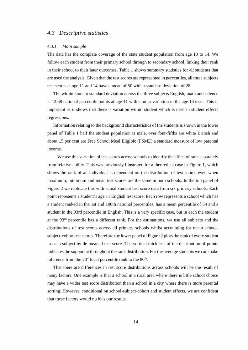
We use this variation of test scores across schools to identify the effect of rank separately

from relative ability. This was previously illustrated for a theoretical case in Figure 1, which

shows the rank of an individual is dependent on the distribution of test scores even when

maximum, minimum and mean test scores are the same in both schools. In the top panel of

Figure 2 we replicate this with actual student test score data from six primary schools. Each

point represents a student’s age 11 English test score. Each row represents a school which has

a student ranked in the 1st and 100th national percentiles, has a mean percentile of 54 and a

student in the 93rd percentile in English. This is a very specific case, but in each the student

at the 93rd percentile has a different rank. For the estimations, we use all subjects and the

distributions of test scores across all primary schools whilst accounting for mean school-

subject-cohort test scores. Therefore the lower panel of Figure 2 plots the rank of every student

in each subject by de-meaned test score. The vertical thickness of the distribution of points

indicates the support at throughout the rank distribution. For the average students we can make

inference from the 20th local percentile rank to the 80th.

That there are differences in test score distributions across schools will be the result of

many factors. One example is that a school in a rural area where there is little school choice

may have a wider test score distribution than a school in a city where there is more parental

sorting. However, conditional on school-subject-cohort and student effects, we are confident

that these factors would no bias our results.

15

4.3.2 Longitudinal Study of Young People in England

Appendix Table 3 shows descriptive statistics for the LSYPE sample which we use to

estimate rank effects on a direct measure of confidence. The LSYPE respondents are

representative of the main sample, although mean age 11 test scores are slightly lower and the

proportion of Free School Meal Eligible is higher than the national at 18.6% and 14.6%

respectively (Appendix Table 3).

The LSYPE students are asked to rate themselves in each of the subjects from ‘Not good

at all’ to ‘Very Good,’ which is summarized in Appendix Table 5. Our measure of confidence

is coarse, with only five categories to choose from and around 60% choosing ‘fairly good’.

We can see that students do think about their own ability, with less than 0.2% not having an

opinion. As would be expected, those who considered themselves to be poor performers did

tend to have lower average national KS2 percentile rank and lower rank within their school.

However, there is also large variance in these ranks within these self-evaluated categories. For

every subject, each self-assessment category with an opinion has at least one individual in the

top 9% nationally, including those who considered themselves ‘Not Good’. Similarly, each

category has an individual in the lowest performing percentile nationally, even those who

consider themselves very good.18

5 Main Results

5.1 Effect of Rank: comparing across school cohorts

To begin the discussion of the results we present estimates of the impact of primary school

rank on age 14 test scores. The estimates are reported in Panel A of Table 2, with the

specifications becoming increasingly flexible moving across columns to the right. The first

row shows estimates of the rank parameter using fully flexible set of controls for age 11 test

scores, allowing each percentile score to have a different effect on later test scores and the

second row instead uses a third order polynomial of age 11 test scores. It appears that this is

sufficient approximation to account for the effect of age 11 test scores. All estimates control

for a set of student characteristics and have standard errors clustered at the secondary school

level.19

18 In Appendix Table 5 we also show the performance of the top and the bottom 10% of students within

each self-assessment category that are less affected by outliers. We continue to see very large variance

within categories. Consider Science in Panel C: of those who consider themselves ‘Very Good’ the

bottom 10% performers in this category are ranked at the 17 percentile point nationally, whereas the

top 10% of performers in the category that rated themselves ‘Not very good at all’ ranked at 64 th

percentile nationally. 19 Student characteristics are ethnicity, gender, ever Free School Meal Eligible (FSME) and Special

Educational Needs (SEN)

16

The first column is a basic specification, which only controls for age 11 test scores, student

characteristics, along with cohort and subject fixed effects. This shows a large effect: a student

at the top of their cohort has an 11.6 larger national percentile rank gain in test scores compared

to a student ranked at the bottom, ceteris paribus. However, this regression does not condition

on school-subject-cohort effects and therefore the parameter cannot be interpreted as pure rank

effect as it will also capture the effects of relative ability. Furthermore, it uses variation in

average quality of students across schools, which might correlate to family background

characteristics, later school quality, and other unobserved variables.

Indeed, column (2) additionally allows for any primary school-subject-cohort effects and

is significantly smaller and (Specification 1). Using this specification, the effect of being

ranked top compared to bottom ceteris paribus is associated with a gain 7.96 national

percentile ranks (0.29 standard deviations) conditional on a cubic of age 11 test scores. This

can be interpreted as the additional ordinal rank effect. Given the distribution of test scores

across schools, very few students would be bottom ranked at one school and top at another

school. A more useful metric is to describe the effect size in terms of standard deviations, a

one standard deviation increase in rank is associated with increases in later test scores by 0.085

standard deviations or 2.36 national percentile points. In comparison with other student

characteristics, females’ growth rate is 1.01 national percentile points higher than males and

free school meal eligible students on average lose 2.96 national percentile points (Appendix

Table 6).20

We see that when additionally allowing for secondary school-subject-cohort effects

(Specification 2) there is only a marginal impact on the estimates and are not significantly

different from those in column 2. This is evidence that that there is negligible sorting into

secondary schools by subject rank, conditional on student test scores. Given that secondary

school attended can be argued to be an outcome, these effects will not be included in the within

student analysis.

5.2 Effect of Rank: within student analysis

We now turn to estimates that use the within student variation to estimate the rank effect

(Specification 3). Conditioning on student effects allows for individual growth rates, which

absorb any student level characteristic. Since students attend the same primary and secondary

school for all subjects, any general school quality or school sorting is also accounted for.

Subject specific primary school quality is absorbed by the primary school-subject-cohort

effects, and allows for longer run impacts of teachers in a subject area. This uses the variation

20 Including the rank parameter in this specification reduces the Mean Square Error by 0.31. This is

more than the reduction from allowing for a gender growth term (0.25) or an ethnicity growth term

(0.28).

17

in the relative growth rates across subjects within student according to differing rank in

primary school.

Besides removing potential biases, the inclusion of student effects changes the

interpretation of the rank parameter. The student effect will also absorb any spillover effects

gained through high ranks in other subjects and is only identifying the relative gains in that

subject. Accordingly the within student estimate is considerably smaller. The effect from

moving to the bottom to top of class ceteris paribus increases national percentile rank by 4.56

percentiles, as we see in Panel A, column (4) of Table 2.

To make a comparison in terms of standard deviations this effect is scaled by the within

student standard deviation of national percentile rank (11.32). Therefore, conditional on

student and school-subject-cohort effects, the maximum effect of rank is 0.40 standard

deviations. This is a very large effect, but a change from last to best rank within student

represents an extreme treatment. It is more conceivable for a student to move 0.5 rank points,

e.g. being at the 25th percentile in one subject and 75th at another. Our estimates imply that this

student would improve their test scores in that subject by 0.20 standard deviations. In terms

of effect size, given that a standard deviation of the rank within student is 0.138 for any one-

standard deviation increase in rank, test scores increase by about 0.056 standard deviations.21

Again, if there were any general gains through achieving a high rank in one subject, this

would be absorbed in the within student estimates, and thus could be interpreted as the

between subject substitutions of effort allocation, or a lower bound of the effect of being

highly ranked. The difference between the within school estimates (7.96) and the within

student estimates (4.56) can be interpreted as an upper bound of the gains from spilovers

between subjects. A more detailed interpretation of the differences in effect size are provided

in Section 7.5 once a mechanisms has been established, and Appendix 3 which describes a

basic model for this mechanism.

5.3 Non-linear Effects

The specifications thus far assumed the effect of rank is linear, however, it is conceivable that

the effects of rank change throughout the rank distribution (Brown, 2011). To address this we

allow for non-linear effects of rank by replacing the rank parameter with a series of 20

indicator variables according to the vingtiles in rank, plus top and bottom of class dummies,

as outlined in specification (4).

The equivalent estimates from specification (1) and (3), i.e. without and with student fixed

effects, are presented in Figure 3. The effect of rank appears to be almost linear throughout

21 For students with similar ranks across subjects the choice of specialization could be less clear.

Indeed, in a sample of the bottom quartile of students in terms of rank differences, the estimated rank

effect is 25% smaller than those from the top quartile. Detailed results available on request.

18

the rank distribution, with small flicks in the tails. In comparison, all rank coefficients are

significantly different from the reference group of the median-ranked students (10th vingtile).

This indicates that the effect of rank exists throughout; even those students ranked just above

the median perform better three years later than those at the median. Given that students are

not informed of rank, our interpretation of this is that students are good at ranking themselves

within the classroom. This ranking developed through the constant exposure to peers over the

length of primary school, which continually reinforces the effect of rank such that by the end

of primary school they have strong beliefs about where they rank.

5.4 Heterogeneity by gender and parental income

We now turn to how the effects of rank vary by student characteristics using the student fixed

effects specification (3) with non-linear rank effects and interacting the rank variable with the

dichotomous characteristic of interest.22 The student characteristics are Male: Female and,

FSME: Non-FSME. The reference group coefficients and the interaction plus reference group

coefficients are plotted to show the effect of rank on test scores for both groups, illustrating

how the different groups react to primary school rank.23

The first panel in Figure 4 shows the how rank relates to the gains in later test scores by

gender. Males are more affected by rank throughout 95% of the rank distribution, this is shown

by the steeper gradient of the rank effect. Males gain four times more from being at the top of

the class, but also lose out marginally more from being in the bottom half. As this is within

student variation in later test scores, and therefore the coefficient could be interpreted as a

specialising term, implying that prior rank has a stronger specialising effect on males than

females. The stronger positive effects for males could also be caused by them perceiving

themselves higher ranked than they actually are, as we are of course estimating the effect of

perceived rank using information on the actual rank.

The second panel in Figure 4 shows that FSME students are less negatively affected by

rank and more positively affected than Non-FSME students. FSME students with a high rank

gain more than Non-FSME students, especially those ranked top in class, who gain almost

twice as much. The finding that FSME students below the median have limited negative

effects could be interpreted as these students do not gain much information about themselves

22 Appendix Table 7 shows linear estimates for all specifications. Interacting student characteristics

rather than estimating the effects separately, ensures that students who attend the same school have the

same relative. Use of interactions is preferred over separate regressions as the school-subject-cohort

effects will be shared across groups and so relative test scores according to that school’s mean will be

the same for both. 23 The student characteristics themselves are not included in the estimations, as they are absorbed by

the student effects. These characteristics interacted by rank, however, are not absorbed by student

effects, because there is variation within the student due to having different ranks in each subject.

19

from this as it may match their existing expectations.. Moreover the shallower gradient for

Non-FSME students could also be interpreted that they are less affected by class rank as these

students may have their academic confidence being more be affected by factors outside of

school.

6 Robustness

Some non-trivial empirical challenges arise when estimating the effect of rank conditional on

test score because we do not independently observe both a students’ rank and a student’s

ability. Instead, we rely on externally marked and nationally standardised tests at the end of

primary school to derive a student’s local rank during primary education and also use this

measure to control for a student’s subject-specific achievement. This may cause problems

relating to the influence of peers, parents and measurement error on test scores.

6.1 Peer Effects

Firstly, given that we are discussing an atypical peer effect, it is important to address the issues

associated with such.24 Any primary school peer effects that have a permanent effect on test

scores do not bias the estimates as they are captured in the end-of-primary school test scores.

Furthermore, we can account for contemporaneous secondary peer quality with the inclusion

of secondary school-subject-cohort effects.

However, if peer effects have a transitory effect on test scores i.e. only current peers matter,

any estimation of the effect of primary rank on age 14 test scores whilst controlling for primary

test scores could be biased. This is to the extent that both the conditioning variable and rank

will be correlated with primary peer effects. The intuition for this is as follows: in the presence

of transitory peer effects, a student with lower quality peers would attain a lower primary

school results than otherwise and also have a higher rank than otherwise. Thus, when

controlling for primary test scores in the estimations, those who previously had low quality

peers would appear to gain more as they now have a new peer group, who on average would

be better. Since rank is negatively correlated with peer quality in primary test scores, it would

appear that those with high rank make the most gains. Therefore having a measure of ability

confounded by transitory peer effects would lead to an upward biased rank coefficient.

This is shown to be the case in Appendix 1, where we create a data generating process in

which we specify that subsequent test scores are not effected by rank. Instead test scores are

only a function of ability and individual linear or non-linear peer effects. To be cautious we

24 The standard reflection problem is not a first order issue in this situation, as students are surrounded

by 87% new peers when they transfer to secondary school, and the rank effect is generated by primary

school peers.

20

allow for these peer effects to be 20 times larger than those found in Lavy et al. (2012). We

simulate these data 1000 times and estimate the rank parameter with different sets of controls.

This shows that not controlling for the primary school peer group generates biased results, but

that this bias is negligible when allowing for mean school-subject-cohort effects, even with

these large non-linear peer effects. These simulations and further discussion can be found in

Appendix 1 and Appendix Table 1.

6.2 Measurement Error

In addition to peer effects, individual test scores may be imperfect measures of inputs up

until that point in time. Given that both rank and test scores will be affected by the same

measurement error, but to different extents according to the heterogeneousness of the test

score distributions, making calculating the size of the bias is intractable. To gauge the extent

of measurement error we again simulate the data assuming 20% of the variation in test scores

is random noise, 70% student ability and 10% school effects, these proportions reflect that

80% of the variance of test scores is within schools and 20% across schools (Appendix 2).

This shows that normally distributed individual-specific measurement error would work

against finding any effects.

The intuition for this is the following: a particular student having a large positive

measurement error would result in both an inflated end-of-primary score and a higher local

rank measure. Both of these would work against finding positive effect of rank on later

outcomes, as we control for prior attainment. This student’s later test scores would be

benchmarked against other students' with the same end of primary result but of higher actual

ability. Since the student only got a high local rank because of the measurement error, this

would downward bias any positive rank effect estimate.

6.3 Is rank just picking up ability?

Our estimates of primary school subject-specific rank are relatively large, given that we are

conditioning prior test scores and individual growth. As rank is highly correlated with student

ability and test scores, there could be a concern that measurement error in the test scores of

ability may be recovered by the rank measurement, if rank is measured with less error than

test scores. This may occur in situations where there are large class effects.

To address this specific measurement error problem of rank having less measurement error

than test scores and thus containing residual ability information, we perform placebo tests.

This involves generating a placebo-rank measure that uses the test scores, but would not reflect

the social comparison experiences of students. To achieve this we re-assigned randomly all

students into primary schools by cohort and re-calculated the ranks that they would have had

21

in these schools with their original age-11 test scores but with peers that they never actually

interacted with. These placebo-ranks are highly correlated with age-11 test scores. If they were

found to be significant determinants of later achievement, this would indicate that rank is

picking up ability not captured in end of primary school outcomes. We re-estimate all the

specifications fifty times using new placebo-ranks each time and present the mean results in

Panel B of Table 2, and the non-linear effects in Figure 3. We find no effects of these placebo

ranks on later test scores. From these simulation results we conclude that our findings are

unlikely to be mechanically driven by measurement error in test scores.

6.4 Are student effects enough? Primary school sorting and parental

occupation

The causal interpretation that we give to estimates relies on the conditional independence

assumption. That a student’s rank needs to be orthogonal to other subject-varying

determinants of a student's later achievement. Given the student effects, the variation need not

be orthogonal to general determinants of the student's achievement, but would need to vary

within a student across subjects. A prime example of this could be the occupational

background of the parents. Children of scientists may have a higher learning curve in science

throughout their academic career for reasons of parental investment or inherited ability.

Similarly children of journalists for English and children of accountants in math. This will not

bias our results as long as conditional on age 11 test scores parental occupation is orthogonal

to primary school rank. Or more broadly, there would be a problem if conditional on other

factors, rank was correlated to subject-varying determinates of future achievement. This might

well be the case if parents strongly aspire for their child to rank top in that subject and so chose

primary schools on this basis and also have a higher academic growth rate in that subject

between the ages 11 and 14.

Typically parents are trying to get their child into the ‘best school’ possible in terms of

average grades. This would work against any positive sorting by rank as higher average

achievement would decrease the probability of their child having a high rank. However, if

parents wanted to maximise their child’s rank in a particular subject, this could bias the results.

In order to do this they would need to know the ability of their child and all potential peers by

subject. This is unlikely to be the case, particularly for such young children who have yet to

enter formal education at age 4. Parents could possibly infer the likely distributions of peer

ability if there is autocorrelation of the student achievement within a primary school. This

means that if parents did know the ability of their child by subject, and the achievement

distributions of primary schools they could potentially select a school on this basis.

22

We test for this by using the LSYPE sample which has information on parental occupation.

All parental occupations are classified into English, math, science, or ‘other’ and then an

indicator variable is created for each student-subject if they have a parent who works in that

field.25 This is taken as an indicator for the parents’ subject preference. We then regress age-

11 test scores on parental occupation, school-subject effects and student effects (Table 3, Panel

A) and find that this measure of parental occupation is a significant predictor of student subject

achievement. Then using rank as the dependent variable we test for a violation of the

orthogonality condition in Panel B of Table 3. Here we see that whilst parental occupation

does predict student achievement by subject, it does not predict rank conditional on test scores.

This implies that parents are not selecting schools on the basis of rank for their child. This

does not rule out other co-varying factors that may bias the results but it provides us with

confidence that this likely large factor does not.

7 Mechanisms

A number of different mechanisms could produce similar results; competitiveness;

environmental favours certain ranks; external (parental) investment by task; students learn

about their ability, improving confidence. In the following, we discuss how each coincides

with the results presented so far.

7.1 Hypothesis 1: Competitiveness

If the goal of individuals was to be better than their peers, maximise rank, this could produce

some of our results, but not the full pattern.

To see this, consider two students of the same ability who attend the same secondary school

but went to primary schools of different peer quality. The student attending the primary school

of low quality peers could provide less effort in their end of primary school tests and still be

ranked top. This student would then achieve lower end of primary school test scores than the

student who faced competition in primary school. At secondary school when they have the

same level of competition, and due to their same ability they will have the same expected age

14 test scores. In our estimation, controlling for prior test scores will make it appear that the

student who faced lower competition and was ranked higher, had larger growth and thus

generate the positive effect of rank.

25 Parental Standard Occupational Classification 2000 grouped in Science, Math, English and Other.

Science (3.5%); 2.1 Science and technology, 2.2 Health Professionals, 2.3.2 Scientific researchers, 3.1

Science and Engineering Technicians. Math (3.1%); 2.4.2 Business And Statistical Professionals, 3.5.3

Business And Finance Associate Professionals. English (1.5%): 2.4.5.1 Librarians, 3.4.1 Artistic and

Literary Occupations, 3.4.3 Media Associate Professionals. Other: Remaining responses.

23

However, if these mechanisms were driving the results, we would only expect to see

these effects near the top of the rank distribution as it only applies to students who far exceed

their peers and so get a lower than would be expected age-11 test scores. All those in the

remainder of the distribution would be applying effort during primary school to gain a higher

rank and so we should not see an effect. However given the result that the rank effect is

approximately linear throughout it is unlikely that this type of competition mechanism is

causing the effect.

It could still be the case that primary school subject rank is positively correlated with

the degree of competitiveness of the student. Then those who are the most competitive increase

their effort the most when entering secondary school and so have higher test score growth.

Note that in the student effects specification any general competitiveness of an individual

would be accounted for, this competiveness would need to vary by subject. As previously

mentioned, any factor that varies by student across subjects conditional on prior test scores

could confound –on in this case, explain- the results.

7.2 Hypothesis 2: The environment favours certain ranks

Another possible explanation for this finding is that the environment could favour the growth

of certain ranks of agents. As an example, one can imagine primary school teachers teaching

to the low ability students if faced with a heterogeneous class group.26 If this were the case,

teachers may design their classes with the needs of the lowest ranked students in mind. This

means that these students would achieve higher age 11 test scores than they otherwise would

have done and students further from the bottom lose out.

What would this mean for the rank effect estimates? Again consider two students of the

same ability who attend to the same secondary school but different primary schools, where

one was top of year. The top student would get less attention during primary school and

therefore get a lower grade than they otherwise would have done. At secondary school they

have the same attention due to their same ability and get the same age 14 test scores. In our

estimation, controlling for prior test scores will make it appear that the top student had higher

growth and thus generate the positive effect of rank. Therefore, teachers teaching to the bottom

student could also generate a positive rank effect.

26 We have run estimations controlling for the within school-subject-cohort variance to take into

account that high variance classes may be more difficult to teach. However, these cannot include school-

subject-cohort or student effects, and thus the estimates should not be cleanly interpreted as ordinal

rank affects. Therefore these specifications only allowed for general school effects or no school effects.

The inclusion of a school-subject-cohort variance into these specifications does not significantly alter

the rank parameter. Our findings can be presented upon request.

24

However, this requires primary school teachers only being effective with lowest ranked

students and secondary school teachers teaching to each ability level equally.27 Moreover, if

the effects are mainly due to the teacher focusing on those of low rank we would not

necessarily expect to see the stark differences by gender, or free school meal status. We saw

that males are more affected by rank than females, which would imply that males are more

negatively affected by having the subject content not tailored to them e.g. top males under-

achieve more during primary but catch up during secondary school. This is conceivable,

however it runs counter to our estimate that males on average have lower growth in test scores

between 11 and 14 (Appendix Table 6). Moreover, this does not also easily explain why free

school meal students up to the middle of the class rankings are not negatively affected by the

focus on the bottom, and those at the top of class are. Given these inconsistences, we have

doubt that his is the dominant reason for the effect.

7.3 Hypothesis 3: External (parental) investment by task

It may not be the students that are applying different effort by subject but that parents of the

students are. Parents can assist the child at home with homework or other extra-curricular

activities. If the parents know that their child is ranked highly in one subject, they might

encourage the child to do more activities and be more specialised in this subject. Note that as

we are controlling for student effects, this must be subject specific encouragement rather than

general encouragement regarding schoolwork. As we have already shown that conditional on

test scores, parental occupation does not predict student rank, this hypothesis assumes parents

react to achieved primary school rank rather than prior preferences.

However, we believe there are two simple observations against this mechanism. Firstly,

whilst some parents may choose to specialise their child, others may want to improve their

child’s weakest subject. If parental investment focused on the weaker subject, this would

reverse the rank effect for these students. To explain the positive rank effect, one would need

to assume that the majority of parents wanted their child to specialise at eleven years of age.

Secondly, parents are unlikely to be accurately informed of their child’s rank in class in the

English context. Teacher feedback to parents will convey some information for the parents to

act upon, such as the student being the best or worst in class, but it is doubtful that they would

be able to discern a difference from being near the middle of the cohort rankings. Our results

27 Note if primary teachers taught to the median student, those at both extremes would lose out.

So instead of a linear effect, we would find a U-shaped curve with both students at the bottom and the

top of the distribution gaining relatively more during secondary school.

25

however, show significantly different effects from the median for all vingtiles with school-

subject-cohort effects.28

7.4 Hypothesis 4: Students learn about their ability

Another possibility is that students use their local rank information to learn about their subject-

specific abilities, and as a result allocate effort accordingly. This is similar to the model

proposed by Ertac (2006) where individuals do not know their own ability and therefore use

their own absolute and relative performance to learn about it. This mechanism does not

change an individual’s education production function, only their perception of it. We will

argue below that this feature allows us to test the learning model

Under the learning hypothesis students additionally use local rank information to make

effort investment decisions across subjects. Assuming students want to maximise grades for

minimum effort they would be applying more effort to those subjects where their perceived

ability is highest.29 However, students with larger differences between local and national

percentile ranks (in absolute terms) would have more distorted information about their true

abilities. These students would then be more likely to misallocate effort across subjects, and

thus achieve lower overall grades, compared to students whose local ranks happen to closely

align with national ranks. This is because this misallocation would lead to inefficient effort

allocation across subjects. Whereas, if the rank effects were caused by actual changes in the

education production function (and not just learning and changes in perceptions), even if local

rank was different from national rank, this would not lead to a misallocation of effort in terms

of maximising grades.

We do not have direct data on perceptions versus reality of costs, however we can test for

misallocation of effort by examining how average grades achieved are correlated with

misinformation. More precisely, we compute a measure of misinformation for students in each

subject using their local rank 𝑅𝑖𝑗𝑠𝑐 = [0,1] and national percentile rank 𝑌𝑖𝑗𝑠𝑐𝑡−1 = [0,100] at

age 11. Both are uniformly distributed and therefore we simply define misinformation

𝑀𝑖𝑠𝑖𝑗𝑠𝑐𝑡−1 as the absolute difference between the two after rescaling percentile rank:

𝑀𝑖𝑠𝑖𝑗𝑠𝑐𝑡−1 = |𝑅𝑖𝑗𝑠𝑐 −𝑌𝑖𝑗𝑠𝑐𝑡−1

100⁄ | , 𝑤ℎ𝑒𝑟𝑒 𝑀𝑖𝑠 = [0,1] (7)

This measure takes the value zero for students where their local rank happens to correspond

exactly to the national rank. A large value, on the other hand, indicates large differences

between local and national rank. Averaging this metric across subjects within student provides

28 Information on the within student comparative advantage by subject would be easier for a teacher to

communicate, and so parents could use this to specialize the student. However, these effects would then

appear less significant in the school-subject-cohort effects specifications. 29 Assuming diminishing returns to effort in each subject so that all effort isn’t allocated into just

one subject.

26

a mean indicator of misinformation for each student. To test directly if a student with a large

amount of disinformation does significantly worse, we use a specification similar to (5) but

with the by subject variation removed as we are examining the effect on average test scores.

We estimate the following specification:

�̅�𝑖𝑗𝑐𝑡 = 𝛽𝑅𝑎𝑛𝑘�̅�𝑖𝑗𝑐𝑡−1 + 𝑓(�̅�𝑖𝑗𝑐𝑡−1) + 𝑋𝑖′𝛽𝑡 + 𝜑𝑗𝑐𝑡 + 𝛽𝑀𝑖𝑠𝑀𝑖𝑠̅̅ ̅̅ ̅

𝑖𝑗𝑐𝑡−1 + 𝜖𝑖𝑗𝑘𝑠𝑐𝑡 (8)

Where 𝜖𝑖𝑗𝑐𝑡 = 𝜏𝑖𝑡 + 휀𝑖𝑗𝑐𝑡

where �̅�𝑖𝑗𝑐𝑡 is average test scores across subjects in period t, �̅� is average rank, 𝜑𝑗𝑐 are

primary school-cohort effects and 𝑀𝑖𝑠̅̅ ̅̅ ̅ the additional misinformation variable. If the amount

of misinformation caused them to misallocate effort over subjects we would expect 𝛽𝑀𝑖𝑠 < 0,

alternatively the null hypothesis local rank causes changes to the actual production function

and 𝛽𝑀𝑖𝑠 = 0.

𝐻1: 𝐿𝑒𝑎𝑟𝑛𝑖𝑛𝑔 𝛽𝑀𝑖𝑠 < 0

𝐻0: 𝑁𝑢𝑙𝑙 𝛽𝑀𝑖𝑠 = 0

We obtain the following estimates using our full sample of 2,271,999 students. For

benchmarking purposes, we first estimate a version of specification (8) without the additional

misinformation variable (Table 4). The effect of average rank on average test score is

estimated at 10.7 and highly statistically significant. Column (2) adds the coefficient for the

effect of misinformation, which is estimated to be small and statistically insignificant whilst

the rank parameter remains almost unchanged. Given this specification we fail to reject the

null hypothesis that the amount of misinformation does not cause students to misallocated

effort. We therefore conclude that the learning mechanism alone is unlikely to generate our

results, though we fully acknowledge the limitations of this test, in particular that we cannot

control for primary-cohort-subject or student fixed effects in this specification.

7.5 Hypothesis 5: Rank position develops confidence

An alternative explanation is that when surrounded by people who perform a task worse

(better) than oneself, one develops a positive (negative) non-cognitive skills such as

confidence in that area30. Applied to our setting, we envisage that students with higher rank

would become more confident academically, moreover this confidence can be subject specific,

so that a student can consider themselves good a school but still bad at math (Marsh et al.,

1988; Yeung et al., 2000). There is also broad agreement in the psychological literature that

academic confidence is most malleable before age 11 (Tiedemann, 2000; Lefot et al., 2010;

30 The psychological-education literature uses the term self-concept, which is formed through our

interactions with the environment and peers (O’Mara et al., 2006). Individuals can have positive or

negative self-concept about different aspects of themselves. Valentine et al. (2004) found that students

with a high self-concept would also develop positive non-cognitive skills such as confidence, resilience,

and perseverance.

27

Rubie-Davis, 2011), which is when we measure rank. The importance of such non-cognitive

skills for both academic attainment and non-academic attainment is now well established

(Heckman and Rubinstein, 2001; Borghans et al., 2008; Lindqvist and Vestman, 2011).

Therefore, another potential mechanism is that an individual’s relative rank in a task

amongst peers affects confidence and this affects the costs of effort for that task. 31 An

exemplary basic behavioural model is provided in Appendix 3 where students want to

maximise total grades for a given total cost of effort, and have differential abilities and costs

of effort for each subject. Students who have a high rank in a subject during primary school

then have a lower cost of effort in that subject in secondary school. This will shift the student’s

iso-cost line out along the axis for this subject and therefore they can reach higher isoquant

and will optimally invest more effort in that subject (Appendix Figure 1, Panel B). If there

were any general gains in confidence, which would reduce the cost of any academic effort and

cause a parallel shift out of the iso-cost line and therefore more effort would be allocated to

all subjects.

This model is consistent with the empirical results found in Section 5. The smaller

estimates from the pupil fixed effects specification (3), will have had any general confidence

effect absorbed and so will only be picking up the effect of within student reallocation of effort

across subjects. Whereas, specification (1) which only contains school-subject-cohort effects,

implicitly allow for spillovers between subjects within a pupil and can so be interpreted as a

culmination of the income and substitution effects of rank across subject and so are

accordingly larger (Appendix Figure 1, Panel C).

To provide evidence for this mechanism we link the administrative data to the Longitudinal

Survey of Yong People in England (LSYPE). We are able to match approximately twelve

thousand students from the survey who answer questions on their confidence in each subject.

This allows us to test directly if rank position within primary school has an effect on this

measure of subject confidence, conditional on attainment. The specifications are equivalent to

(1) and (3) with the dependent variable now being student confidence. Since this survey was

only run for one cohort, the school-subject-cohort effects are replaced by school-subject

effects.

Panel A of Table 5 presents these results and demonstrates that conditional on age 11 test

scores students with a higher primary school rank position are significantly more likely to say

that they are good in that subject (column 1). Controlling for school-subject effects, the impact

of moving from the bottom of class to the top is 0.196 points on a five point scale (-2, 2), or

31 Confidence may instead affect a student’s ability in a task rather than cost of effort. This would lead

to the same predicted changes in the effort ratios and empirical results. If we had time use data we

would be able to differentiate between these causes, however given the data available, we are unable to

determine if it is costs or abilities that are affected.

28

about twenty per cent of a standard deviation in our confidence measure (see column 2).32

This suggests that students develop a clear sense of their strengths and weaknesses depending

on their local rank position, conditional on relative test scores.

While we would prefer to have a measure of student confidence directly at age 11 at the

end of primary school, these measures are only available to us just prior to the age 14 tests.

Therefore, in Panel B we additionally control for contemporaneous attainment at age 14,

which is an outcome. To cautiously interpret these estimates, students with ‘the same’ age 11

and 14 results have more confidence if they have had a higher local rank in that subject in

primary school.

Note column (2), the specifications allowing for primary-subject effects cannot reject the

null hypothesis that rank has no effect on confidence. A reason for this is that there are few

students per primary school in this survey (4.5 students conditional on at least one student

being in the survey); as the survey was conducted at secondary schools. The small number of

students per school severely limits the degrees of freedom in each school-subject group, the

lack of variation is exacerbated due to the coarseness of the confidence variable.

To obtain a clearer view of the effect of rank on contemporaneous confidence we estimate

how rank based on age-14 test scores within a secondary school subject affects subject

confidence conditional on secondary-subject effects and individual effects. The advantage of

this is that there are on average 20 students for each school that has students in the survey.33

These results can be found in Panel C, where we see that conditional on school-subject effects,

moving from bottom to top of class improves confidence by 0.43 on the 5 point scale.

Allowing for individuals to have different levels of confidence and only using the variation

between subjects reduces the parameter to 0.38 but remains significant at 1% (column 3).

Furthermore, we examine the heterogeneity of these effects by estimating the effect of age

14 rank on confidence separately by gender, conditional on student and school-subject effects

(lower part of Panel C). We find that the effect on male confidence is five times larger than

the effect on females (�̂�𝑟𝑎𝑛𝑘 𝑚𝑎𝑙𝑒 =0.61, �̂�𝑟𝑎𝑛𝑘 𝑓𝑒𝑚𝑎𝑙𝑒 =0.12), which mirrors the results we

find for the effect of rank on later test scores. Unfortunately due to the smaller sample size of

the LSYPE, we are unable to produce the effects non-linearly or by FSME status.

The magnitudes of the secondary school ranks effects on secondary confidence are large,

but we may expect the contemporaneous effect of primary rank on confidence at age 11 to be

even larger, as academic confidence is thought to be more malleable at this age (Tiedemann,

32 The standard deviation of the confidence measure is 0.99. 33 The reason why we do not look at the effect of KS3 rank on later outcomes is due to the tracking by

subject in secondary school, which will be related to rank. This is not an issue with primary school rank,

because even if there were tracking in primary schools, when moving to secondary school, students

with the same test scores (but different primary ranks) would be assigned to the same track.

29

2000; Lefot et al., 2010; Rubie-Davis 2011). Moreover, we find indicative evidence that later

confidence is affected by previous primary school rank.

Overall given the effects of rank on direct measures of student confidence and the

heterogeneity of effects found in the main results we are confident in our conclusion that

confidence forms according to rank position and that this affects later investment decisions.

8 Conclusions

Individuals continuously make social comparisons, which can affect their beliefs and

investment decisions. If individuals make these comparisons using ordinal as well as cardinal

information, then an individual’s perceived rank amongst their peers could impact on their

actions and later productivity.

This paper examined how, conditional on relative achievement, rank amongst peers affects

subsequent performance. Applied to an education setting we establish a new result that

perceived rank position within primary school has significant effects on secondary school

achievement. Moreover, a higher rank also improves important non-cognitive skills such as

confidence. These rank effects are in addition to any effect caused by a student’s relative

distance from the class mean.

The approximately linear impact of rank implies that students are very good at determining

their rank amongst their peers. Furthermore, there is significant heterogeneity in the effect of

rank with males being influenced considerably more. Correspondingly we find male

confidence in a subject is five times more affected by their rank amongst their peers compared

to females. We cannot fully exclude other mechanisms, such as learning about ability, to

generate parts of these results. However, testing for the impact of misinformation speaks in

favour of mechanisms that change an individual’s education production.

The finding that higher peer quality could have negative effects on later outcomes may seem

counter intuitive, but there are a number of topics in education that have findings which

corroborate this hypothesis.

Research on selective schools and school integration have shown mixed results from

students attending selective or predominantly non-minority schools (Angrist and Lang, 2004;

Clark 2010; Cullen, et al., 2006; Kling et al., 2007). Many of these papers use a regression

discontinuity design to compare the outcomes of the students that just passed the entrance

exam to those that just failed. The common puzzle is that many papers find no benefit from

attending these selective schools. However, our findings would speak to why the potential

benefits of prestigious schools may be attenuated through the development of a fall in

confidence amongst these marginal/bussed students, who necessarily would also be the low

ranked students. This is consistent with Cullen et al. (2006), who find that those whose peers

30

improve the most gain the least: ‘lottery winners have substantially lower class ranks

throughout high school as a result of attending schools with higher achieving peers and are

more likely to drop out’. Similar effects are found in the Higher Education literature with

respect to affirmative action policies (Arcodiacono et al., 2012; Robles and Krishna, 2012).

The early formation of confidence and specialisation could also partly explain why some

achievement gaps increase over the education cycle. Widening overall education gaps have

been documented by race (Fryer and Levitt, 2006; Hanushek and Rivkin 2006; 2009), small

differences in early overall attainment could negatively affect general academic confidence,

which would lead to decreased investment in education and exacerbate any initial differences.

In the case of gender a gap occurs by subject, where males are overly represented in

mathematics and science by the age of 18, despite girls outperforming boys at early ages in

these subjects (Burgess et al, 2004; Machin & McNally, 2005). Even with girls performing

better in all subjects, if boys do comparatively less badly in mathematics and are more affected

by rank for investment decisions, then they would chose to invest more in those subjects.

Finally the literature on age-effects in education shows that older children do better compared

to their younger peers (i.e. Black et al., 2011). Again their relatively higher rank amongst their

cohort my increase their confidence and exacerbate any underlying differences due to age and

is a potential mechanism for the continuation of these effects as the students grow older.

What are the policy implications of these findings? With specific regards to education,

these findings leads to a natural question for a parent deciding on where to send their child (in

partial equilibrium). Should my child attend a ‘prestigious school’ or a ‘worse school’ where

she will have a higher rank? Rank is just one of many factors in the education production

function, and therefore choosing solely on the basis of rank is unlikely to be correct. The

authors are currently not aware of any study that identifies the effectiveness of schools in

terms of standard deviations;34 therefore, we use estimates of the impact of teachers as an

indicative measure for effects of school quality for this benchmarking exercise. A teacher who

is one standard deviation better than average improves student test scores by 0.1 to 0.2

standard deviations (Aaronson, et al. 2007; Rivkin et al. 2005). Comparatively we find that a

student with one standard deviation higher rank in primary school will score 0.08 standard

deviations better at age 14.35

We believe these findings have general implications for productivity and informational

transparency. To improve productivity it would be optimal for managers or teachers to

34 Evaluations of school effectiveness using admission lotteries (i.e. Hoxby et al. 2009, Angrist et al.

2010, Dobbie and Fryer 2011, Abdulkadiroglu et al. 2011) are comparing effectiveness between types

rather than the whole distribution of effectiveness. 35 Note that these are still not directly comparable because the effect of the teacher is annual and quickly

fades out, whereas the rank treatment lasts the duration of primary school (5 years) and the effect is

found three years later.

31

highlight an individual’s local rank position if that individual had a high local rank. If an

individual is in a high-performing peer group and therefore may have a low local rank but a

high global rank a manager should make the global rank more salient. For individuals who

have low global and local ranks, managers should focus on absolute attainment, or focus on

other tasks where the individual has higher ranks.

Finally these findings have general implications regarding the formation of non-cognitive

skills and productivity. Given the heterogeneous effects of rank it would be possible to

organise groups by individuals characteristics and abilities to maximise output. However this

would be very cumbersome and administratively intensive. Therefore the key implication is

that non-cognitive skills such as confidence, perseverance and resilience have large effects on

productivity. Rank can be thought of as just one treatment that impacts on these behaviours,

however there are many other interventions that could have positive effects on all individuals

within a group and not just those above the median.

32

References

Aaronson, D., Barrow, L. and Sander, W. (2007). Teachers and student achievement in the

Chicago public high schools, Journal of Labor Economics, 25(1), pp. 95–135.

Abdulkadiroglu, A., Angrist, J., Dynarski, S., Kane, T., and Pathak, P. (2011). Account-ability

and flexibility in public schools: Evidence from Boston's charters and pilot, The Quarterly

Journal of Economics, 126(2), pp. 699-748.

Angrist, J. (2013). The Perils of Peer Effects, NBER Working Paper No. 19774.

Angrist, J and Lang, K. (2004). Does School Integration Generate Peer Effects? Evidence from

Boston's Metco Program, American Economic Review, 94(5), pp. 1613-1634.

Angrist, J., Dynarski, S., Kane, T., Pathak, P., and Walters, C. (2010). Inputs and impacts in

charter schools: KIPP Lynn, American Economic Review, 100(2), pp. 239-243.

Arciciacono, P., Aucejo, E. and Spenner, K. (2012). What Happens After Enrolement? An

Analysis of the Time Path of Racial Differences in GPA and Major Choice, IZA Journal of

Labor Economics, 1(5).

Azmat, G, and Iriberri N. (2010) The importance of relative performance feedback information:

Evidence from a natural experiment using high school students, Journal of Public Economics,

94(7–8), pp. 435-452.

Beyer, S. (1990) Gender Differences in the accuracy of self-evaluations of performance. Journal

of Personality and Social Psychology, 58, pp.960-970.

Black, S. E., Devereux, P. J. and Salvanes, K. G. (2011). Too Young to Leave the Nest? The

Effects of School Starting Age, The Review of Economics and Statistics, 93(2), pp. 455–467.

Borghans, L., Duckworth A., Heckman J., Weel ter Bas (2008). The Economics and Psychology

of Personality Traits, Journal of Human Resources, 43(4), pp.872-1059.

Brown G., Gardner, J., Oswald, A. and Qian, J. (2008). Does Wage Rank Affect Employee’s

Well-being?, Industrial Relations, 47(3), pp. 355-389.

Brown J., (2011). Quitters Never Win: The (Adverse) Incentive Effects of Competing with

Superstars, Journal of Political Economy, 119(5), pp. 982-1013.

Burgess S., McConnell B., Propper C., Wilson D., Girls Rock, Boys Roll: An Analysis of the

Age 14-16 Gender Gap in English Schools, Scottish Journal of Political Economy, Scottish

Economic Society, 51(2), pp. 209-229.

Card, D., Mas, M., Moretti, E., and Saez, E. (2012). Inequality at Work: The Effect of Peer

Salaries on Job Satisfaction, American Economic Review, 102(6), pp.2981-3003.

33

Carrell, S.E., Fullerton R.L., and West, J.E. (2009). Does Your Cohort Matter? Estimating Peer

Effects in College Achievement, Journal of Labour Economics, 27(3), pp.439-464.

Clark, A., and Oswald, A. (1996). Satisfaction and Comparison Income, Journal of Public

Economics, 61(September), pp. 359-381.

Clark, A., Masclet, D. and Villeval M.C., (2010). Effort and comparison income: experiment and

survey evidence, Industrial and Labour Relations Review, 63(3) pp. 407-426.

Clark, D. (2010) Selective Schools and Academic Achievement The B.E. Journal of Economic

Analysis and Policy, 10(1), pp. 1935-1682.

Cullen, J.B., Jacob, B.A. and Levitt S., (2006). The effect of school choice on participants:

evidence from randomised lotteries, Econometrica, 74(5), pp.1191-1230.

DFE (2011). Class Size and education in England evidence report, Research Report DFE-RR169.

Dobbie, W. and Fryer, R. (2011). Are high quality schools enough to close the achievement gap?

Evidence from the Harlem Children's Zone, American Economic Journal: Applied Economics,

3(3), pp. 158-187.

Eriksson, T., Poulsen, A., Villeval, M., (2009). Feedback and incentives: experimental evidence,

Labour Economics, 16, pp. 679–688.

Falk, A., Ichino, A., (2006) Clean evidence on peer pressure Journal of Labor Economics 24 (1),

pp. 39–57

Festinger, L. (1954). A theory of social comparison processes Human Relations, 7, pp. 117–140.

Fryer, G. and Levitt, S. (2006). The Black-White Test Score Gap Through Third Garde, American

Law and Economics Review, 8(2), pp. 249-281.

Genakos, C. and Paglierio M. (2012) Interim Rank, Risk Taking, and Performance in Dynamic

Tournaments. Journal of Political Economy, University of Chicago Press, vol. 120(4), pages

782 - 813.

Guimaraes, P. and Portugal, P. (2010) A Simple Feasible Alternative Procedure to Estimate

Models with High-Dimensional Fixed Effects, Stata Journal, 10(4), pp. 628-649.

Hanushek, E. (2006). School Resources, Handbook of the Economics of Education, 2(Chapter

14).

Hanushek, E., Kain, J. and Rivkin, S. (2005). Teachers, Schools, and Academic Achievement,

Econometrica, 73(2), pp. 417–458.

Hanushek, E. and Rivkin, S. (2006). School Quality and the Black-White Achievement Gap,

NBER Working Paper No. 12651.

34

Hanushek, E. and Rivkin, S. (2009). Harming the Best: How Schools Affect the Black-White

Achievement Gap, Journal of Policy Analysis and Management, 28(3), pp. 336-393.

Heckman J., Stixrud, J. and Urzua, S. (2006). The Effects of Cognitive and Noncognitive Abilities

on Labor Market Outcomes and Social Behavior, Journal of Labor Economics, 24(3), pp. 411-

482.

Hoxby, C. (2001). If Families Matter Most, Where Do Schools Come In? in T. Moe, ed. A Primer

on American Schools. Stanford: Hoover Institution Press.

Hoxby, C., Murarka, S., and Kang, J. (2009). How New York City's charter schools affect

achievement, Cambridge, MA: New York City Charter Schools Evaluation Project.

Forest J. J., and Heath C. (1996) The Evaluation Gap in Performance Perceptions:

Illusory Perceptions of Groups and Individuals” Journal of Applied Psychology, 81(4), pp.

369-379

Kenny, D. A. (1991). A general model of consensus and accuracy in interpersonal perception.

Psychological Review, 98, pp. 155-163.

Kling, J., Liebman, J. and Katz, L. (2007). Experimental Analysis of Neighborhood Effects,

Econometrica, 25(1), pp. 83-119.

Kosfeld, M. and Neckermann, S. (2011). Getting More Work for Nothing? Symbolic Awards and

Worker Performance, American Economic Journals: Microeconomics, 3(3), pp. 86-99.

Lavy, V., Silva, O. and Weinhardt, F. (2012). The Good, The Bad and The Average: Evidence

on Ability Peer Effects in Schools, Journal of Labor Economics, 20(2), pp.367-414.

Lindqvist, E., and Vestman, R., 2011. The Labor Market Returns to Cognitive and Noncognitive

Ability: Evidence from the Swedish Enlistment, American Economic Journal: Applied

Economics, 3(1), pp. 101-28.

Littlepage, G., Robison, W., & Reddington, K. (1997). Effects of task experience and group

experience on group performance, member ability, and recognition of expertise.

Organizational Behavior and Human Decision Processes, 69, pp. 133-147.

Machin, S., and McNally, S. (2005). Gender and student achievement in English schools, Oxford

review of economic policy, 21(3). pp. 357-372.

Manski, C. (1993). Identification of Endogenous Social Effects: The Reflection Problem, The

Review of Economic Studies, 60(3), pp. 531-542.

Marsh, H., Byrne, B. and Shavelson, R. (1988). A multifaceted academic self-concept: Its

hierarchical structure and its relation to academic achievement, Journal of Educational

Psychology, 80, pp.366–380.

35

Mas, A. and Moretti, E., (2009). Peers at work, American Economic Review, 99(1), pp. 112–145.

Nickell, S. (1981). Biases in Dynamic Models with Fixed Effects, Econometrica, 49(6), pp. 1417-

1426.

Page, M., Carrell, S., and West, J. (2010). Sex and Science: How Professor Gender Affects the

Gender Gap, Quarterly Journal of Economics, 125(3), pp.1101-1144.

Paulhus, D. L., & Bruce, M. N. (1992). The effect of acquaintanceship on the validity of

personality impressions: A longitudinal study. Personality Processes and Individual

Differences, 63, pp. 816-824

Parducci, A (1965). Category Judgment: A Range-frequency Theory, Psychological Review,

(72), pp. 407-418.

Robles, F. V.C. and Krishna, K. (2012). Affirmative Action in Higher Education in India:

Targeting, Catch Up, and Mismatch, NBER Working paper No.17727.

Tiedemann, J. (2000). Parents' gender stereotypes and teachers' beliefs as predictors of children's

concept of their mathematical ability in elementary school, Journal of Educational

Psychology, 92(1), pp 144-151.

Todd, P.E. and Wolpin K.I., (2003). On The Specification and Estimation of The Production

Function for Cognitive Achievement, The Economic Journal, 113(1), pp. 3-33.

Tversky A. and Kahneman, D., (1974). Judgment under Uncertainty: Heuristics and Biases,

Science, 185(4157), pp. 1124-1131.

Valentine, J., DuBois, D. and Cooper, H. (2004). The relations between self-beliefs and academic

achievement: A systematic review, Educational Psychologist, (39), pp.111–133.

Watkins, M., Lei, P. and Canivez, L. (2007). Psychometric intelligence and achievement: A cross-

lagged panel analysis, Intelligence, 35, pp.59-68.

Yeung, A. and Lee, F. (1999). Self-concept of high school students in China: Confirmatory factor

analysis of longitudinal data, Educational and Psychological Measurement, 59, pp.431–450.

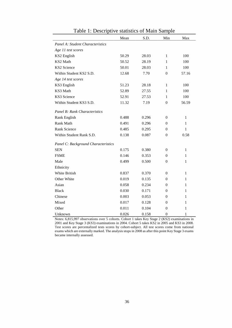
36

Table 1: Descriptive statistics of Main Sample

Mean S.D. Min Max

Panel A: Student Characteristics

Age 11 test scores

KS2 English 50.29 28.03 1 100

KS2 Math 50.52 28.19 1 100

KS2 Science 50.01 28.03 1 100

Within Student KS2 S.D. 12.68 7.70 0 57.16

Age 14 test scores

KS3 English 51.23 28.18 1 100

KS3 Math 52.89 27.55 1 100

KS3 Science 52.91 27.53 1 100

Within Student KS3 S.D. 11.32 7.19 0 56.59

Panel B: Rank Characteristics

Rank English 0.488 0.296 0 1

Rank Math 0.491 0.296 0 1

Rank Science 0.485 0.295 0 1

Within Student Rank S.D. 0.138 0.087 0 0.58

Panel C: Background Characteristics

SEN 0.175 0.380 0 1

FSME 0.146 0.353 0 1

Male 0.499 0.500 0 1

Ethnicity

White British 0.837 0.370 0 1

Other White 0.019 0.135 0 1

Asian 0.058 0.234 0 1

Black 0.030 0.171 0 1

Chinese 0.003 0.053 0 1

Mixed 0.017 0.128 0 1

Other 0.011 0.104 0 1

Unknown 0.026 0.158 0 1

Notes: 6,815,997 observations over 5 cohorts. Cohort 1 takes Key Stage 2 (KS2) examinations in

2001 and Key Stage 3 (KS3) examinations in 2004. Cohort 5 takes KS2 in 2005 and KS3 in 2008.

Test scores are percentalized tests scores by cohort-subject. All test scores come from national

exams which are externally marked. The analysis stops in 2008 as after this point Key Stage 3 exams

became internally assessed.

37

Table 2: Age 14 Test Scores on Primary School Rank (Age 11)

Raw

(1)

Primary

(2)

Primary-

Secondary

(3)

Primary-

Student

(4)

Panel A: The effect of primary rank

Primary Rank

Flexible Age 11 Test Scores

11.551** 7.662** 10.415** 4.402**

0.293 0.145 0.146 0.132

Primary Rank

Cubic Age 11 Test Scores

11.001** 7.960** 7.901** 4.562**

0.298 0.145 0.146 0.132

Panel B: The effect of placebo rank

Placebo Rank

Flexible Age 11 Test Scores

0.006 0.015 0.014 0.009

0.100 0.011 0.131 0.123

Placebo Rank

Cubic Age 11 Test Scores

0.005 0.013 0.016 -0.008

0.100 0.116 0.119 0.137

Student characteristics Abs

Age 11 Test Scores

Primary-cohort-subject Effects

Secondary Effects Abs Abs

Secondary-cohort-subject Effects

Student Effects

Notes: Results obtained from twelve separate regressions based on 2,271,999 student observations and

6,815,997 student-subject observations. The dependent variable is by cohort by subject percentalized KS3

test scores. All specifications control for Key Stage 2 results, student characteristics, cohort effects and

subject effects. Student characteristics are ethnicity, gender, free school meal (FSME) and special

educational needs (SEN). Coefficients in columns (2) and (3) are estimated using Stata command reg2hdfe

allowing two high dimensional fixed effects to be absorbed. Standard errors in italics and clustered at 3,800

secondary schools. Abs indicates that the effect is absorbed by another estimated effect. ** 1% sig.

38

Table 3: Balancing by Parental Occupation

Primary

(1)

Primary-

Student

(2)

Panel A: Effects on age-11 tests

Parental Occupation 7.722** 1.706*

0.840 0.783

Panel B: Effects on Ordinal Rank

Parental Occupation -0.004 0.000

0.005 0.034

Primary-subject Effects

Student Effects

Notes: Results obtained from regressions based on 31,050 subject-student observations

for which parental occupations could be identified from the LSYPE. Detailed

occupational coding available from the authors on request. Panel A has KS2 as

dependent variable, in Panel B KS2 with polynomials up to cubic are included as

controls. All regressions control for student characteristics and subject effects.

Regressions in column (2) estimated using Stata command reg2hdfe. ** 1%,* 5%

significant.

Table 4: Average Age 14 Test Scores on Average Primary School Rank

(Age 11) and Misinformation

Raw

(1)

Primary

(2)

Primary Rank

10.710** 10.694**

0.223 0.223

Misinformation

- -0.361

- 0.233

Student characteristics

Age 11 Test Scores (cubic)

Primary-cohort Effects

Notes: Results obtained from two separate regressions based on 2,271,999 student

observations averaged over subjects where column (2) includes an additional

explanatory variable on misinformation. The dependent variable is by cohort by

subject percentalized average KS3 test scores. The misinformation measurement is

the average absolute difference between local rank and national percentile rank for

each student. Student characteristics are ethnicity, gender, free school meal (FSME)

and special educational needs (SEN). Coefficients are estimated using Stata

command reg2hdfe allowing two high dimensional fixed effects to be absorbed.

Standard errors in italics and clustered at 3,800 secondary schools. ** 1% sig.

39

Table 5: Student Confidence on Rank (1) (2) (3)

Panel A: Subject Confidence on Age 11 Test Scores

Primary Rank 0.563** 0.196* 0.056

0.038 0.117 0.18

Panel B: Subject Confidence on Age 11 & 14 Test Scores

Primary Rank 0.436** 0.109 0.014

0.039 0.115 0.079

Panel C: Subject Confidence on Age 14 Test scores

Secondary Rank 0.897** 0.427** 0.382**

0.048 0.099 0.155

Secondary Rank – Male Students 0.754*** 0.530*** 0.606***

0.059 0.126 0.206

Secondary Rank – Female Students 1.067*** 0.317* 0.115

0.071 0.166 0.233

School-by-subject effects

Student Effects

Notes: Results obtained from fifteen separate regressions based on 11,558 student observations and 34,674

student-subject observations from the LSYPE sample (17,415 female, 17,259 male). For descriptives, see

Appendix Table 3. The dependent variable is a course measure of confidence by subject. All specifications in

columns 1 and 2 control for observable student characteristics, these are absorbed by the student effect in

column 3. Student characteristics are ethnicity, gender, free school meal (FSME) and special educational needs

(SEN).Panels A and B condition on age 11 test scores (cubic) and primary school by subject effects. Panels B

and C condition on age 14 test scores (cubic) and secondary school by subject effects. Cohort effects are not

included because the LSYPE data is only available for one cohort. Standard errors in parenthesis and clustered

at 796 secondary schools ** 1% sig. * 10% sig.

40

Figure 1: Rank Dependent on Distribution Given Absolute and Relative

Score

Notes: This figure illustrates that students with the same test score relative to the group mean can have

different ranks depending on the distribution of test scores. Two cohorts of eleven students are

represented, with each mark representing a student’s test score. Test scores are increasing from left to

right. Each cohort has the same minimum, maximum and mean test scores. Cohort A has a unimodal

distribution and Cohort B has a bimodal test score distribution. A student with a test score of X in Cohort

A would have a lower rank than the same test score in Cohort B. Similarly a test score of Y would be

ranked differently in Cohorts A and B. Given the definition of rank given in Section 5.2, the rank

measurements for score X are 𝑅𝑥𝐴= 0.1 and 𝑅𝑥𝐵= 0.4 and for Y are 𝑅𝑦𝐴= 0.9, 𝑅𝑦𝐵= 0.6. This is based on

the illustration from Brown et al. (2008).

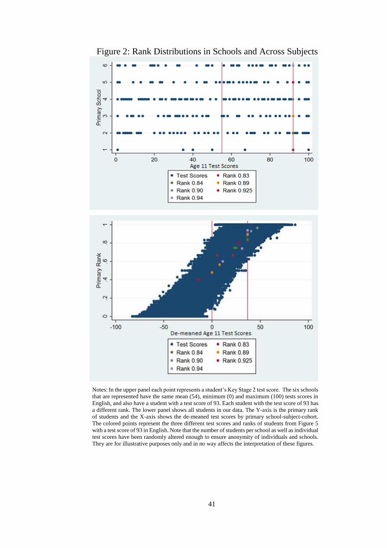
41

Figure 2: Rank Distributions in Schools and Across Subjects

Notes: In the upper panel each point represents a student’s Key Stage 2 test score. The six schools

that are represented have the same mean (54), minimum (0) and maximum (100) tests scores in

English, and also have a student with a test score of 93. Each student with the test score of 93 has

a different rank. The lower panel shows all students in our data. The Y-axis is the primary rank

of students and the X-axis shows the de-meaned test scores by primary school-subject-cohort.

The colored points represent the three different test scores and ranks of students from Figure 5

with a test score of 93 in English. Note that the number of students per school as well as individual

test scores have been randomly altered enough to ensure anonymity of individuals and schools.

They are for illustrative purposes only and in no way affects the interpretation of these figures.

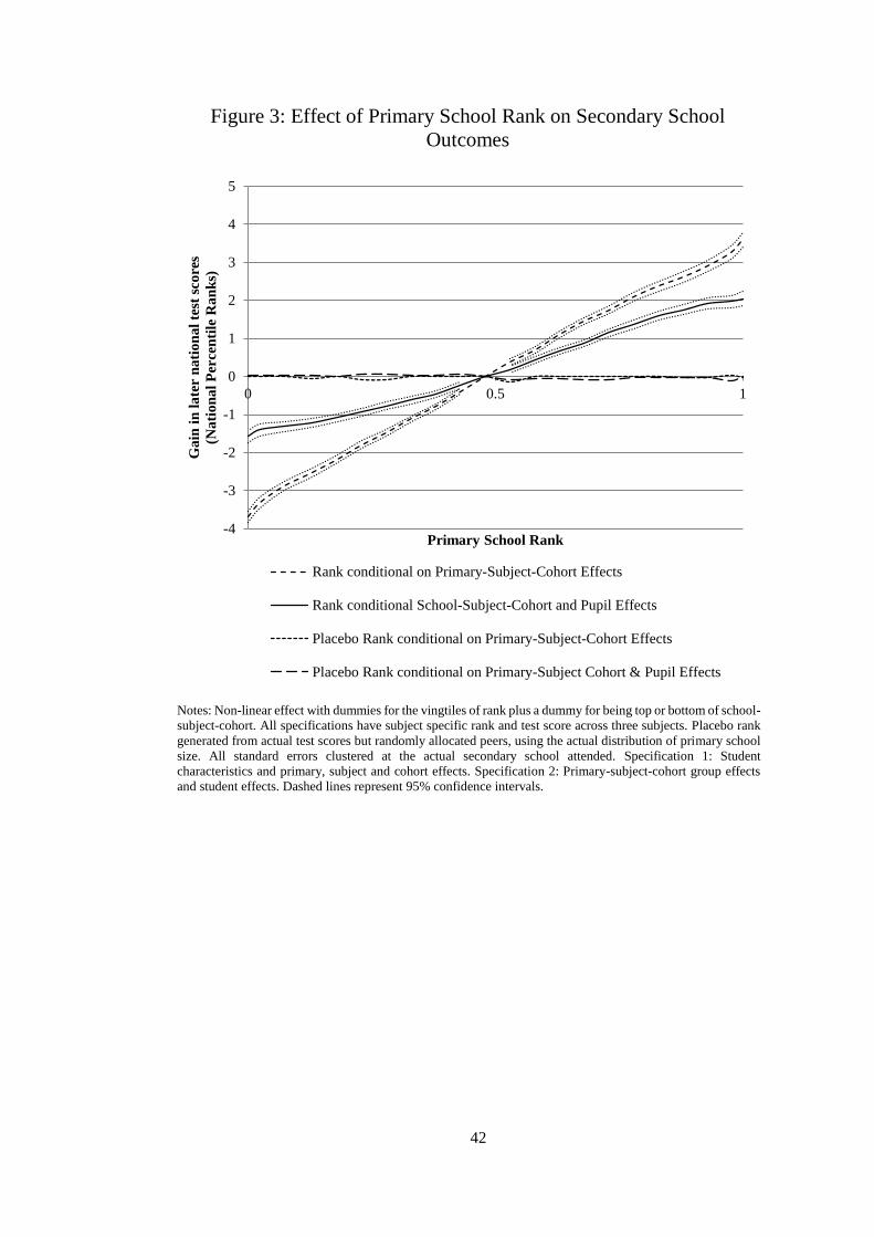
42

Figure 3: Effect of Primary School Rank on Secondary School

Outcomes

Notes: Non-linear effect with dummies for the vingtiles of rank plus a dummy for being top or bottom of school-

subject-cohort. All specifications have subject specific rank and test score across three subjects. Placebo rank

generated from actual test scores but randomly allocated peers, using the actual distribution of primary school

size. All standard errors clustered at the actual secondary school attended. Specification 1: Student

characteristics and primary, subject and cohort effects. Specification 2: Primary-subject-cohort group effects

and student effects. Dashed lines represent 95% confidence intervals.

-4

-3

-2

-1

0

1

2

3

4

5

0 0.5 1

Ga

in i

n l

ate

r n

ati

on

al

test

sco

res

(Na

tio

na

l P

erce

nti

le R

an

ks)

Primary School Rank

Rank conditional on Primary-Subject-Cohort Effects

Rank conditional School-Subject-Cohort and Pupil Effects

Placebo Rank conditional on Primary-Subject-Cohort Effects

Placebo Rank conditional on Primary-Subject Cohort & Pupil Effects

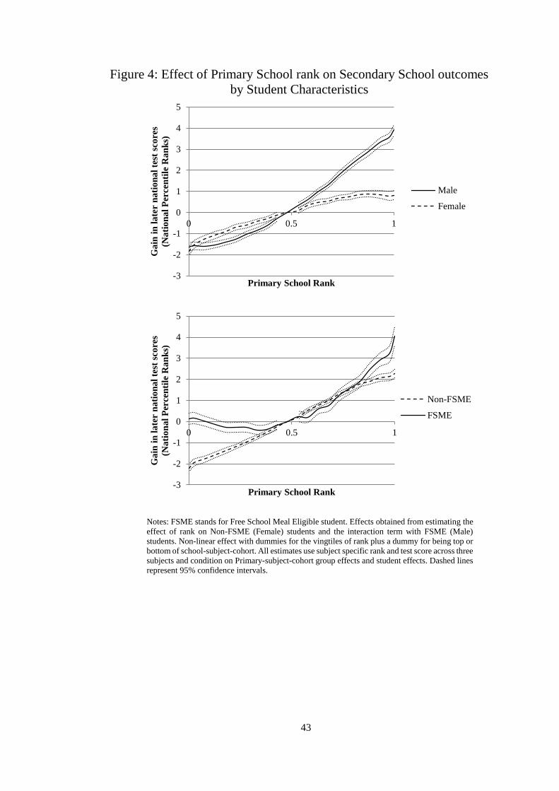
43

Figure 4: Effect of Primary School rank on Secondary School outcomes

by Student Characteristics

Notes: FSME stands for Free School Meal Eligible student. Effects obtained from estimating the

effect of rank on Non-FSME (Female) students and the interaction term with FSME (Male)

students. Non-linear effect with dummies for the vingtiles of rank plus a dummy for being top or

bottom of school-subject-cohort. All estimates use subject specific rank and test score across three

subjects and condition on Primary-subject-cohort group effects and student effects. Dashed lines

represent 95% confidence intervals.

-3

-2

-1

0

1

2

3

4

5

0 0.5 1

Ga

in i

n l

ate

r n

ati

on

al

test

sco

res

(Na

tio

na

l P

erce

nti

le R

an

ks)

Primary School Rank

Male

Female

-3

-2

-1

0

1

2

3

4

5

0 0.5 1

Ga

in i

n l

ate

r n

ati

on

al

test

sco

res

(Na

tio

na

l P

erce

nti

le R

an

ks)

Primary School Rank

Non-FSME

FSME

44

Appendix 1: Peer Effects

There are concerns that with the existence of peer effects, peer quality jointly determines both

a student’s rank position, as well as their age 11 results. This mechanical relationship could

potentially bias our estimation. This is because in the presence of peer effects a student with

lower quality peers would attain a lower age 11 test scores than otherwise and also have a

higher rank than otherwise. Thus, when controlling for prior test scores in the age 14

estimations, when students have a new peer group, those who previously had low quality peers

in primary school would appear to gain more. Since rank is negatively correlated with peer

quality in primary, it would appear that those with high rank make the most gains. Therefore,

having a measure of ability confounded by peer effects would lead to an upward-biased rank

coefficient.

This situation could be present in our data. We propose a resolution through the inclusion

of subject-by-cohort-by-primary school controls. These effects will absorb any average peer

effects within a classroom. However, they will not absorb any peer effects that are individual

specific. This is because all students will have a different set of peers (because they cannot be

a peer to themselves). Therefore, including class level controls will only remove the average

class peer effect. The remaining bias will be dependent on the difference between the average

peer effect and the individual peer effect and its correlation with rank. We are confident that

the remaining effect of peers on the rank parameter will be negligible, given that the difference

between average and individual peer effect decreases as class size increases. The bias will be

further attenuated because the correlation between the difference and rank will be less than

one, and both effects are small.

We test this by running simulations of a data generating process where test scores are not

affected by rank and are only a function of ability and school/peer effects; we then estimate

the rank parameter given this data. We allow for the data-generating process to have linear

mean-peer effects, as well as non-linear peer effects (Lavy et al. 2012). We are conservative

and assume extremely large peer effects, allowing both types of peer effects to account for

10% of the variance of a student’s subject-specific outcome. Given that the square root of the

explained variance is the correlation coefficient, this assumption implies that a one standard

deviation increase in peer quality improves test scores by 0.31 standard deviations. In reality

Lavy et al. (2012) find a 1sd increase in peers only increases test scores by 0.015standard

deviations, a 20th of the size.

The data generating process is as follows:

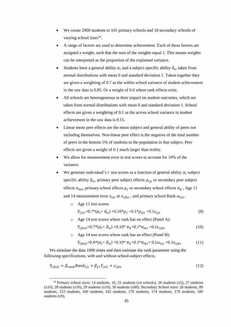
45

We create 2900 students to 101 primary schools and 18 secondary schools of

varying school sizes36.

A range of factors are used to determine achievement. Each of these factors are

assigned a weight, such that the sum of the weights equal 1. This means weights

can be interpreted as the proportion of the explained variance.

Students have a general ability 𝛼𝑖 and a subject specific ability 𝛿𝑖𝑠 taken from

normal distributions with mean 0 and standard deviation 1. Taken together they

are given a weighting of 0.7 as the within school variance of student achievement

in the raw data is 0.85. Or a weight of 0.6 where rank effects exist.

All schools are heterogeneous in their impact on student outcomes, which are

taken from normal distributions with mean 0 and standard deviation 1. School

effects are given a weighting of 0.1 as the across school variance in student

achievement in the raw data is 0.15.

Linear mean peer effects are the mean subject and general ability of peers not

including themselves. Non-linear peer effect is the negative of the total number

of peers in the bottom 5% of students in the population in that subject. Peer

effects are given a weight of 0.1 much larger than reality.

We allow for measurement error in test scores to account for 10% of the

variance.

We generate individual’s i test scores as a function of general ability 𝛼𝑖 subject

specific ability 𝛿𝑖𝑠, primary peer subject effects 𝜌𝑖𝑗𝑠 or secondary peer subject

effects 𝜎𝑖𝑘𝑠, primary school effects 𝜇𝑗 or secondary school effects 𝜋𝑘 , Age 11

and 14 measurement error 휀𝑖𝑗𝑠 or 𝜖𝑖𝑗𝑘𝑠 , and primary school Rank 𝜔𝑖𝑗𝑠.

o Age 11 test scores

𝑌𝑖𝑗𝑠1=0.7*(𝛼𝑖+ 𝛿𝑖𝑠) +0.10*𝜇𝑗 +0.1*𝜌𝑖𝑗𝑠 +0.1휀𝑖𝑗𝑠 (9)

o Age 14 test scores where rank has no effect (Panel A):

𝑌𝑖𝑗𝑘𝑠2=0.7*(𝛼𝑖+ 𝛿𝑖𝑠) +0.10* 𝜋𝑘+0.1*𝜎𝑖𝑘𝑠 +0.1𝜖𝑖𝑗𝑘𝑠 (10)

o Age 14 test scores where rank has an effect (Panel B):

𝑌𝑖𝑗𝑘𝑠2=0.6*(𝛼𝑖+ 𝛿𝑖𝑠) +0.10* 𝜋𝑘+0.1*𝜎𝑖𝑘𝑠+ 0.1𝜔𝑖𝑗𝑠 +0.1𝜖𝑖𝑗𝑘𝑠 (11)

We simulate the data 1000 times and then estimate the rank parameter using the

following specifications, with and without school-subject effects.

𝑌𝑖𝑗𝑘𝑠2 = 𝛽𝑟𝑎𝑛𝑘𝑅𝑎𝑛𝑘𝑖𝑗𝑠 + 𝛽𝑦1𝑌𝑖𝑗𝑠1 + 휀𝑖𝑗𝑘𝑠 (12)

36 Primary school sizes; 14 students, 16, 25 students (x4 schools), 26 students (x5), 27 students

(x10), 28 students (x10), 29 students (x10), 30 students (x60). Secondary School sizes: 26 students, 89

students, 153 students, 160 students, 162 students, 170 students, 174 students, 178 students, 180

students (x9),

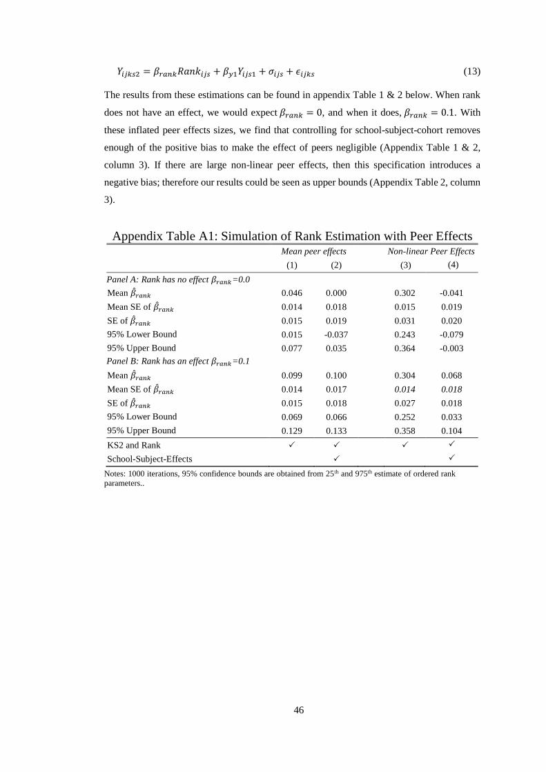
46

𝑌𝑖𝑗𝑘𝑠2 = 𝛽𝑟𝑎𝑛𝑘𝑅𝑎𝑛𝑘𝑖𝑗𝑠 + 𝛽𝑦1𝑌𝑖𝑗𝑠1 + 𝜎𝑖𝑗𝑠 + 𝜖𝑖𝑗𝑘𝑠 (13)

The results from these estimations can be found in appendix Table 1 & 2 below. When rank

does not have an effect, we would expect 𝛽𝑟𝑎𝑛𝑘 = 0, and when it does, 𝛽𝑟𝑎𝑛𝑘 = 0.1. With

these inflated peer effects sizes, we find that controlling for school-subject-cohort removes

enough of the positive bias to make the effect of peers negligible (Appendix Table 1 & 2,

column 3). If there are large non-linear peer effects, then this specification introduces a

negative bias; therefore our results could be seen as upper bounds (Appendix Table 2, column

3).

Appendix Table A1: Simulation of Rank Estimation with Peer Effects Mean peer effects Non-linear Peer Effects

(1) (2) (3) (4)

Panel A: Rank has no effect 𝛽𝑟𝑎𝑛𝑘=0.0

Mean �̂�𝑟𝑎𝑛𝑘 0.046 0.000 0.302 -0.041

Mean SE of �̂�𝑟𝑎𝑛𝑘 0.014 0.018 0.015 0.019

SE of �̂�𝑟𝑎𝑛𝑘 0.015 0.019 0.031 0.020

95% Lower Bound 0.015 -0.037 0.243 -0.079

95% Upper Bound 0.077 0.035 0.364 -0.003

Panel B: Rank has an effect 𝛽𝑟𝑎𝑛𝑘=0.1

Mean �̂�𝑟𝑎𝑛𝑘 0.099 0.100 0.304 0.068

Mean SE of �̂�𝑟𝑎𝑛𝑘 0.014 0.017 0.014 0.018

SE of �̂�𝑟𝑎𝑛𝑘 0.015 0.018 0.027 0.018

95% Lower Bound 0.069 0.066 0.252 0.033

95% Upper Bound 0.129 0.133 0.358 0.104

KS2 and Rank

School-Subject-Effects

Notes: 1000 iterations, 95% confidence bounds are obtained from 25th and 975th estimate of ordered rank

parameters..

47

Appendix 2: Measurement Error in Test Scores

Test scores are scores are an imprecise measure of ability. Could this measurement error be

driving the results? Given that rank and test scores will both be affected by the same

measurement error (but to different extents due to heterogeneous test score distributions across

classes), calculating the size of the bias is intractable. To gauge the potential effect of

measurement error, we simulate the data generating process. This allows us to have a true

measure of ability and a student test score of which 20% of the variation is measurement error.

Comparing the estimates of the rank parameter both with and without measurement error

provides us an indication of the extent to which measurement error could be driving the results.

Rank measurement is then derived from the noisy test score measure in both cases.

The data generating process is as follows:

2900 students to 101 primary schools and 18 secondary schools of varying

sizes37.

A range of factors are used to determine achievement. Each of these factors are

assigned a weight, such that the sum of the weights equal 1. This means weights

can be interpreted as the proportion of the explained variance.

Students have a general ability 𝛼𝑖 and a subject specific ability 𝛿𝑖𝑠 taken from

normal distributions with mean 0 and standard deviation 1. Taken together they

are given a weighting of 0.7 as the within school variance of student achievement

in the raw data is 0.85. Or a weight of 0.6 where rank effects exist.

All schools are heterogeneous in their impact on student outcomes, which are

taken from normal distributions with mean 0 and standard deviation 1. School

effects are given a weighting of 0.1 as the across school variance in student

achievement in the raw data is 0.15.

We allow for measurement error in test scores to account for 20% of the

variance, double the effect of any school subject effects.

We generate individual’s i test scores as a function of general ability 𝛼𝑖 subject

specific ability 𝛿𝑖𝑠, primary school effects 𝜇𝑗 or secondary school effects 𝜋𝑘 ,

Age 11 and 14 measurement error 휀𝑖𝑗𝑠 or 𝜖𝑖𝑗𝑘𝑠 , and primary school Rank 𝜔𝑖𝑗𝑠

o Age 11 test scores

𝑌𝑖𝑗𝑠1=0.7*(𝛼𝑖+ 𝛿𝑖𝑠) +0.10*𝜇𝑗 +0.2휀𝑖𝑗𝑠 (14)

37 Primary school sizes; 14 students, 16, 25 students (x4 schools), 26 students (x5), 27 students (x10),

28 students (x10), 29 students (x10), 30 students (x60). Secondary School sizes: 26 students, 89

students, 153 students, 160 students, 162 students, 170 students, 174 students, 178 students, 180

students (x9),

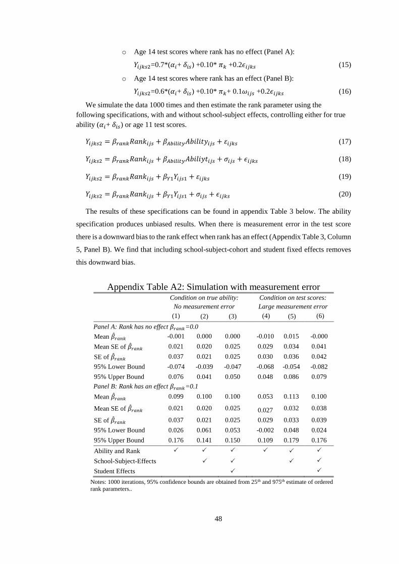
48

o Age 14 test scores where rank has no effect (Panel A):

𝑌𝑖𝑗𝑘𝑠2=0.7*(𝛼𝑖+ 𝛿𝑖𝑠) +0.10* 𝜋𝑘 +0.2𝜖𝑖𝑗𝑘𝑠 (15)

o Age 14 test scores where rank has an effect (Panel B):

𝑌𝑖𝑗𝑘𝑠2=0.6*(𝛼𝑖+ 𝛿𝑖𝑠) +0.10* 𝜋𝑘+ 0.1𝜔𝑖𝑗𝑠 +0.2𝜖𝑖𝑗𝑘𝑠 (16)

We simulate the data 1000 times and then estimate the rank parameter using the

following specifications, with and without school-subject effects, controlling either for true

ability (𝛼𝑖+ 𝛿𝑖𝑠) or age 11 test scores.

𝑌𝑖𝑗𝑘𝑠2 = 𝛽𝑟𝑎𝑛𝑘𝑅𝑎𝑛𝑘𝑖𝑗𝑠 + 𝛽𝐴𝑏𝑖𝑙𝑖𝑡𝑦𝐴𝑏𝑖𝑙𝑖𝑡𝑦𝑖𝑗𝑠 + 휀𝑖𝑗𝑘𝑠 (17)

𝑌𝑖𝑗𝑘𝑠2 = 𝛽𝑟𝑎𝑛𝑘𝑅𝑎𝑛𝑘𝑖𝑗𝑠 + 𝛽𝐴𝑏𝑖𝑙𝑖𝑡𝑦𝐴𝑏𝑖𝑙𝑖𝑦𝑡𝑖𝑗𝑠 + 𝜎𝑖𝑗𝑠 + 𝜖𝑖𝑗𝑘𝑠 (18)

𝑌𝑖𝑗𝑘𝑠2 = 𝛽𝑟𝑎𝑛𝑘𝑅𝑎𝑛𝑘𝑖𝑗𝑠 + 𝛽𝑌1𝑌𝑖𝑗𝑠1 + 휀𝑖𝑗𝑘𝑠 (19)

𝑌𝑖𝑗𝑘𝑠2 = 𝛽𝑟𝑎𝑛𝑘𝑅𝑎𝑛𝑘𝑖𝑗𝑠 + 𝛽𝑌1𝑌𝑖𝑗𝑠1 + 𝜎𝑖𝑗𝑠 + 𝜖𝑖𝑗𝑘𝑠 (20)

The results of these specifications can be found in appendix Table 3 below. The ability

specification produces unbiased results. When there is measurement error in the test score

there is a downward bias to the rank effect when rank has an effect (Appendix Table 3, Column

5, Panel B). We find that including school-subject-cohort and student fixed effects removes

this downward bias.

Appendix Table A2: Simulation with measurement error

Condition on true ability:

No measurement error

Condition on test scores:

Large measurement error

(1) (2) (3) (4) (5) (6)

Panel A: Rank has no effect 𝛽𝑟𝑎𝑛𝑘=0.0

Mean �̂�𝑟𝑎𝑛𝑘 -0.001 0.000 0.000 -0.010 0.015 -0.000

Mean SE of �̂�𝑟𝑎𝑛𝑘 0.021 0.020 0.025 0.029 0.034 0.041

SE of �̂�𝑟𝑎𝑛𝑘 0.037 0.021 0.025 0.030 0.036 0.042

95% Lower Bound -0.074 -0.039 -0.047 -0.068 -0.054 -0.082

95% Upper Bound 0.076 0.041 0.050 0.048 0.086 0.079

Panel B: Rank has an effect 𝛽𝑟𝑎𝑛𝑘=0.1

Mean �̂�𝑟𝑎𝑛𝑘 0.099 0.100 0.100 0.053 0.113 0.100

Mean SE of �̂�𝑟𝑎𝑛𝑘 0.021 0.020 0.025 0.027 0.032 0.038

SE of �̂�𝑟𝑎𝑛𝑘 0.037 0.021 0.025 0.029 0.033 0.039

95% Lower Bound 0.026 0.061 0.053 -0.002 0.048 0.024

95% Upper Bound 0.176 0.141 0.150 0.109 0.179 0.176

Ability and Rank

School-Subject-Effects

Student Effects

Notes: 1000 iterations, 95% confidence bounds are obtained from 25th and 975th estimate of ordered

rank parameters..

49

Appendix 3: Model of Effort Allocation

To explicitly describe the mechanism, we put forward a basic behavioural model of how rank

could affect later actions through changes in confidence. There are two stages, a learning stage

followed by an action stage. In the learning stage, individuals of heterogeneous ability in

different tasks are randomly allocated into groups. They perform tasks and compare their

abilities relative to others in their group. This forms their task specific and a general

confidence. In the second stage, individuals are put into a new peer group in which they

perform the same tasks. The confidence formed in the first stage affects their costs of effort

for each task in the second stage.38 Individuals now allocate effort to each task to maximise

output for a given level of effort and ability. In this simplified model we assume that

individuals do not include later rank directly in their objective function.

Without losing generality, we apply this to the education setting where students vary in

ability across subjects and are randomly allocated to primary schools where their confidence

in each subject if formed during the first stage. This is generated through students interacting

with their peers, such as observing who answers questions, and teacher grading. For the

purposes of the model, we assume that students exert no effort during primary school, with

outcomes being a product of ability and school factors.

In the second stage, we model students as grade maximising agents for a given total cost

of effort 𝑇𝑖 and subject ability level 𝐴𝑖𝑠. The grade achieved Y, by a student i in subject s is a

function of ability 𝐴𝑖𝑠 and effort 𝐸𝑖𝑠 according to a to a separable production function where

there are decreasing returns to effort in each subject, 0<κ<1. For simplicity of notation, assume

that there are only two subjects, s ={e, m}. The productivity of effort is additionally effected

by subject specific school factors 𝜇𝑠. The total test score of individual i is the sum of this

function over subjects, therefore, for student i in school 𝜇𝑖𝑠 the education production is:

𝑌𝑖 = 𝑓(𝐴𝑖𝑒 , 𝐸𝑖𝑒) + 𝑓(𝐴𝑖𝑚 , 𝐸𝑖𝑚) = 𝜇𝑖𝑒 ∙ 𝐴𝑖𝑒 ∙ 𝐸𝑖𝑒κ + 𝜇𝑖𝑚 ∙ 𝐴𝑖𝑚 ∙ 𝐸𝑖𝑚

κ (21)

This can be rearranged in terms of 𝐸𝑖𝑒 so that an isoquant (𝑄𝑜) can be drawn for a given

total grades 𝑌𝑖, subject abilities and school effects, all the combinations of subject effort (see

Figure 1).

𝐸𝑖𝑒 = (𝑌𝑖−𝜇𝑖𝑚∙𝐴𝑖𝑚∙𝐸𝑖𝑚

κ

𝜇𝑖𝑒∙𝐴𝑖𝑒 )

1

κ (22)

A student’s confidence in each subject that was generated in the first stage, determines the

student’s cost of effort. Those with more confidence will find the cost of effort lower. For

38 Confidence instead affect an agent’s ability in a task rather than cost of effort. This would lead to the

same predicted changes in the effort ratios and empirical results. Given the data available, we are unable

to determine if it is costs or abilities that are affected. With information on time allocated on each task

a positive relationship with rank would imply cost reductions, whereas no changes or decreases would

imply gains in ability. We have chosen costs, as this is the more parsimonious and intuitive of the two.

50

example when faced with a difficult mathematics question, a student who considers herself

good at mathematics would spend longer looking for a solution, compared to another student

who may give up. Therefore, the cost of subject effort 𝑐𝑠 is a decreasing function of school

subject rank 𝑅𝑠, 𝐶𝑠 = 𝑔(𝑅𝑠) 𝑤ℎ𝑒𝑟𝑒 𝑔′ < 0. We assume costs of subject effort are linear in

effort applied to that subject. We also allow for a general cost of effort 𝐶𝑖𝑔, which varies across

individuals according to general academic confidence and is a decreasing function of ranks in

all subjects, 𝐶𝑔 = 𝑑(𝑅𝑚, 𝑅𝑒) 𝑤ℎ𝑒𝑟𝑒 𝑑′(𝑅𝑠) < 0 for s={m,e}. This general cost function

reflects a student’s general attitude towards education, and is linear in the sum of effort applied

across all subjects, 𝐸𝑖𝑚 + 𝐸𝑖𝑒 . The total cost of effort 𝑇 that a student can apply is fixed,

however the inclusion of a general cost of academic effort term, means that the total effort

applied by a student is very flexible.

𝑇𝑖 ≥ 𝐶𝑖𝑚 ∙ 𝐸𝑖𝑚 + 𝐶𝑖𝑒 ∙ 𝐸𝑖𝑒 + 𝐶𝑖𝑔 ∙ (𝐸𝑖𝑚 + 𝐸𝑖𝑒) (23)

This allows for an isocost line to be drawn using the cost of effort in each subject as the

factor prices for a given total effort (see Figure 1, Panel A). There is additionally a non-binding

time constraint, normalising the total time available to one, 𝐸𝑖𝑒 + 𝐸𝑖𝑚 < 1. As standard, the

solution is where the technical rate of substitution equals the relative factor prices i.e. where

the isoquant and isocost lines are tangential.

Therefore student i wants to maximise total grades by solving:

max𝐸𝑒𝐸𝑚

𝑌(𝐸𝑒 , 𝐸𝑚) = 𝑓(𝐸𝑒) + 𝑓(𝐸𝑚)

= 𝜇𝑒 ∙ 𝐴𝑒 ∙ 𝐸𝑒κ + 𝜇𝑚 ∙ 𝐴𝑚 ∙ 𝐸𝑚

κ (24)

𝑠. 𝑡. 𝑇 ≥ 𝐶𝑒 ∙ 𝐸𝑒 + 𝐶𝑚 ∙ 𝐸𝑚 + 𝐶𝑔 ∙ (𝐸𝑚 + 𝐸𝑒) (25)

1 > 𝐸𝑒 + 𝐸𝑚

𝑙 = 𝑌 − 𝜆(𝑇 − 𝐶𝑒𝐸𝑒 − 𝐶𝑚𝐸𝑚 − 𝐶𝑔 ∙ (𝐸𝑚 + 𝐸𝑒))

𝑑𝑙

𝑑𝐸𝑒= 0 →

𝜕𝑌

𝜕𝐸𝑒= 𝜆(𝐶𝑒 + 𝐶𝑔)

𝑑𝑙

𝑑𝐸𝑚= 0 →

𝜕𝑌

𝜕𝐸𝑚= 𝜆(𝐶𝑚 + 𝐶𝑔)

𝑑𝑙

𝑑𝜆= 0 → 𝐶𝑒𝐸𝑖𝑒 + 𝐶𝑚𝐸𝑚 + 𝐶𝑔 ∙ (𝐸𝑚 + 𝐸𝑖𝑒) = 𝑇

𝑑𝑌

𝑑𝐸𝑠= κ ∙ 𝜇𝑠 ∙ 𝐴𝑠 ∙ 𝐸𝑠

κ−1

Therefore

κ ∙ 𝜇𝑠 ∙ 𝐴𝑠 ∙ 𝐸𝑠κ−1 = 𝜆 (𝐶𝑠 + 𝐶𝑔)

Where λ reflects the marginal grade per effort and λ>0

51

κ ∙ 𝜇𝑒 ∙ 𝐴𝑒𝐸𝑒κ−1

(𝐶𝑒 + 𝐶𝑔)= 𝜆 =

κ ∙ 𝜇𝑚 ∙ 𝐴𝑚𝐸𝑚κ−1

(𝐶𝑚 + 𝐶𝑔)

This gives

(𝐶𝑒+𝐶𝑔)

(𝐶𝑚+𝐶𝑔)=

𝜇𝑒∙𝐴𝑒∙𝐸𝑒κ−1

𝜇𝑚∙𝐴𝑚∙𝐸𝑚κ−1 (26)

It is also clear that given this specification effort exerted in a specific subject is dependent on

the student’s ability and cost of effort in that subject and general confidence.

𝐸𝑖𝑠∗ = (

𝜆(𝐶𝑖𝑠+𝐶𝑔)

κ∙𝜇𝑠∙𝐴𝑖𝑠)

1

κ−1 (27)

In the above λ reflects the marginal grade per effort where λ>0. As costs are decreasing in

subject rank and 0 < κ <1 any increase in rank in subject s will increase the later effort

allocated to that subject. A student who increases their confidence in English would now have

a lower cost of learning English and therefore increase their English to math effort ratio. The

reduced costs also induce an income effect as more effort can be allocated for the same total

effort costs. The isocost line shifts outwards and a higher isoquant can be reached (Figure 1

Panel B). This student would now optimally chose to exert more effort in English (𝐸1 > 𝐸0)

and less effort in math (𝑀1 < 𝑀0). As a result, the total grades that can be achieved for a

given cost of effort and ability level is higher.

This has yet to take into account the reduction in general academic costs of effort 𝐶𝑔, due

to an increase in general academic confidence. This would reduce the cost for both subjects,

and so there would only be an income effect. This shifts the isocost curve out, increasing the

maximum possible English and Math effort that could be allocated (Figure 1 Panel C). Given

this specification, the final effect on math effort is ambiguous, as it depends on the shape and

position on the isoquants and the importance of general confidence.

For the estimations that used the variation in rank within student, the individual effects

absorb any individual general academic confidence gained by being ranked highly. These

estimations are therefore equivalent to the case where 𝐶𝑔 is fixed and we’re just looking at

the effect allocation across subjects. The specifications that do not include individual effects

and instead use the within class variation do allow for spillover effects between subjects and

so there can be general gains in confidence. This is the intuition for why the parameters

recovered from the student effects estimations are smaller than those from the school cohort

effect estimations. This two-subject example is for exposition only but easily extends to the

setting where an individual is maximising total grades over three subjects.

52

Appendix Figure A1: Optimal Allocation of Effort Panel A

Panel B

Panel C

Isoquant 𝑄0:

𝐸𝑒0 = (𝑌0−𝜇𝑚∙𝐴𝑚∙𝐸𝑚0

κ

𝜇𝑒∙𝐴𝑒 )

1

κ

Optimal English effort 𝐸𝑒0 and math effort 𝐸𝑚0,

given cost of English and math effort 𝐶𝑒𝑜, 𝐶𝑚𝑜.

Marginal cost of effort equals marginal test

score gain where isoquant and isocost curve are

tangential.

Isoquant 𝑄1:

𝐸𝑒1 = (𝑌1−𝜇𝑚∙𝐴𝑚∙𝐸𝑚1

κ

𝜇𝑒∙𝐴𝑒 )

1

κ

A higher rank in English, improves English

confidence and reduces cost of effort in

English 𝐶𝑒0>𝐶𝑒1. Shifts isocost line out to new

intercept on English axis. Increase English

effort 𝐸𝑒0 < 𝐸𝑒1 and decrease math effort

𝐸𝑚𝑜 > 𝐸𝑚1

Isoquant 𝑄2:

𝐸𝑒2 = (𝑌1−𝜇𝑚∙𝐴𝑚∙𝐸𝑚2

κ

𝜇𝑒∙𝐴𝑒 )

1

κ

A higher rank in English, also improves general

confidence and reduces cost of effort in both

subjects 𝐶𝑠1>𝐶𝑠2. Shifts isocost line out to new

intercept on both axis. This increases effort

applied in both subjects 𝐸𝑠1 < 𝐸𝑠2.

Total effects: More effort applied to English

𝐸𝑒2 > 𝐸𝑒0, ambiguous effect on math.

53

Table A3: Descriptive Statistics of LSYPE Sample

Mean S.D. Min Max

Panel A: Student Characteristics

Age 11 test scores

KS2 English 49.48 27.77 1 100

KS2 Math 50.11 28.37 1 100

KS2 Science 48.69 28.30 1 100

Within Student KS2 S.D. 12.71 7.69 0 47.44

Age 14 test scores

KS3 English 50.67 28.00 1 100

KS3 Math 52.99 27.61 1 100

KS3 Science 52.21 27.71 1 100

Within Student KS3 S.D. 12.71 7.69 0 47.44

Panel B: Rank Characteristics

Rank English 0.491 0.295 0 1

Rank Math 0.496 0.297 0 1

Rank Science 0.482 0.294 0 1

Within Student Rank S.D. 0.140 0.086 0 0.49

Panel C: Background Characteristics

SEN 0.166 0.372 0 1

FSME 0.186 0.389 0 1

Male 0.498 0.500 0 1

Ethnicity

White British 0.651 0.477 0 1

Other White 0.026 0.159 0 1

Asian 0.175 0.380 0 1

Black 0.081 0.273 0 1

Chinese 0.002 0.048 0 1

Mixed 0.002 0.046 0 1

Other 0.035 0.184 0 1

Unknown 0.028 0.164 0 1

Notes: 34,674 observations from the cohort who took KS2 in 2001 and KS3 in 2004. Test

scores are percentalized tests scores by cohort-subject.

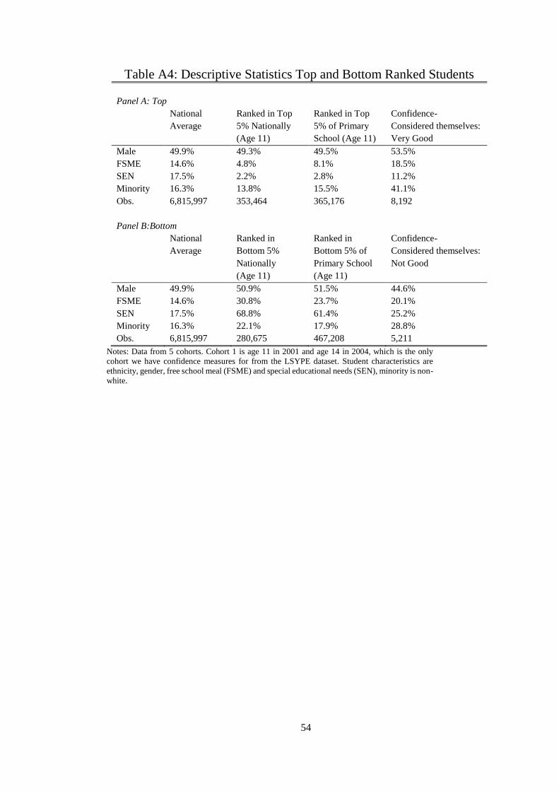
54

Table A4: Descriptive Statistics Top and Bottom Ranked Students

Panel A: Top

National

Average

Ranked in Top

5% Nationally

(Age 11)

Ranked in Top

5% of Primary

School (Age 11)

Confidence-

Considered themselves:

Very Good

Male 49.9% 49.3% 49.5% 53.5%

FSME 14.6% 4.8% 8.1% 18.5%

SEN 17.5% 2.2% 2.8% 11.2%

Minority 16.3% 13.8% 15.5% 41.1%

Obs. 6,815,997 353,464 365,176 8,192

Panel B:Bottom

National

Average

Ranked in

Bottom 5%

Nationally

(Age 11)

Ranked in

Bottom 5% of

Primary School

(Age 11)

Confidence-

Considered themselves:

Not Good

Male 49.9% 50.9% 51.5% 44.6%

FSME 14.6% 30.8% 23.7% 20.1%

SEN 17.5% 68.8% 61.4% 25.2%

Minority 16.3% 22.1% 17.9% 28.8%

Obs. 6,815,997 280,675 467,208 5,211

Notes: Data from 5 cohorts. Cohort 1 is age 11 in 2001 and age 14 in 2004, which is the only

cohort we have confidence measures for from the LSYPE dataset. Student characteristics are

ethnicity, gender, free school meal (FSME) and special educational needs (SEN), minority is non-

white.

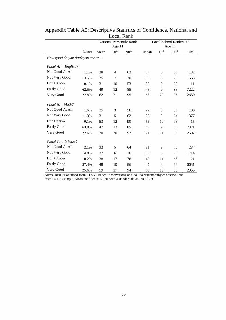
55

Appendix Table A5: Descriptive Statistics of Confidence, National and

Local Rank

National Percentile Rank

Age 11

Local School Rank*100

Age 11

Share Mean 10th 90th Mean 10th 90th Obs.

How good do you think you are at…

Panel A: …English?

Not Good At All 1.1% 28 4 62 27 0 62 132

Not Very Good 13.5% 35 7 70 33 3 73 1563

Don't Know 0.1% 31 10 53 35 0 63 11

Fairly Good 62.5% 49 12 85 48 9 88 7222

Very Good 22.8% 62 21 95 63 20 96 2630

Panel B:…Math?

Not Good At All 1.6% 25 3 56 22 0 56 188

Not Very Good 11.9% 31 5 62 29 2 64 1377

Don't Know 0.1% 53 12 90 56 10 93 15

Fairly Good 63.8% 47 12 85 47 9 86 7371

Very Good 22.6% 70 30 97 71 31 98 2607

Panel C:…Science?

Not Good At All 2.1% 32 5 64 31 3 70 237

Not Very Good 14.8% 37 6 76 36 3 75 1714

Don't Know 0.2% 38 17 76 40 11 68 21

Fairly Good 57.4% 48 10 86 47 8 88 6631

Very Good 25.6% 59 17 94 60 18 95 2955

Notes: Results obtained from 11,558 student observations and 34,674 student-subject observations

from LSYPE sample. Mean confidence is 0.91 with a standard deviation of 0.99.

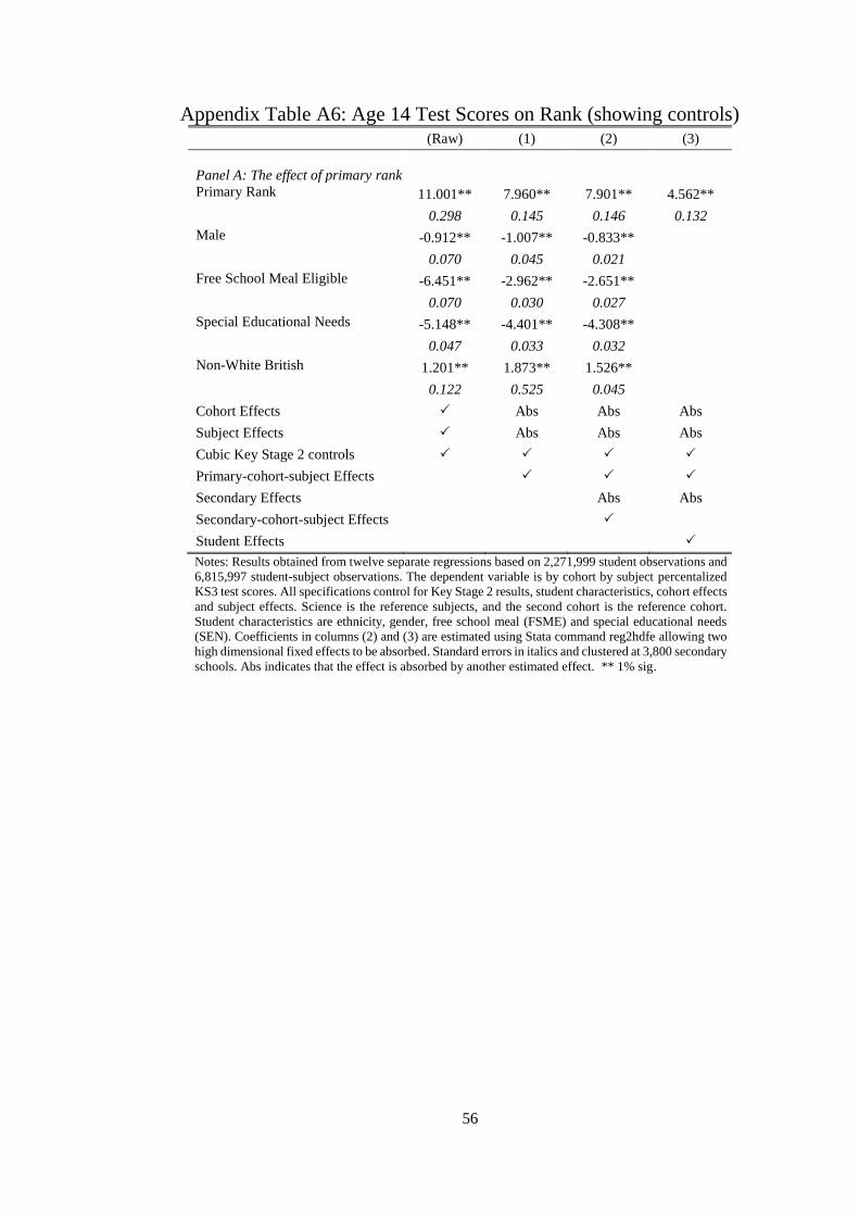
56

Appendix Table A6: Age 14 Test Scores on Rank (showing controls) (Raw) (1) (2) (3)

Panel A: The effect of primary rank Primary Rank 11.001** 7.960** 7.901** 4.562**

0.298 0.145 0.146 0.132

Male -0.912** -1.007** -0.833**

0.070 0.045 0.021

Free School Meal Eligible -6.451** -2.962** -2.651**

0.070 0.030 0.027

Special Educational Needs -5.148** -4.401** -4.308**

0.047 0.033 0.032

Non-White British 1.201** 1.873** 1.526**

0.122 0.525 0.045

Cohort Effects Abs Abs Abs

Subject Effects Abs Abs Abs

Cubic Key Stage 2 controls

Primary-cohort-subject Effects

Secondary Effects Abs Abs

Secondary-cohort-subject Effects

Student Effects

Notes: Results obtained from twelve separate regressions based on 2,271,999 student observations and

6,815,997 student-subject observations. The dependent variable is by cohort by subject percentalized

KS3 test scores. All specifications control for Key Stage 2 results, student characteristics, cohort effects

and subject effects. Science is the reference subjects, and the second cohort is the reference cohort.

Student characteristics are ethnicity, gender, free school meal (FSME) and special educational needs

(SEN). Coefficients in columns (2) and (3) are estimated using Stata command reg2hdfe allowing two

high dimensional fixed effects to be absorbed. Standard errors in italics and clustered at 3,800 secondary

schools. Abs indicates that the effect is absorbed by another estimated effect. ** 1% sig.

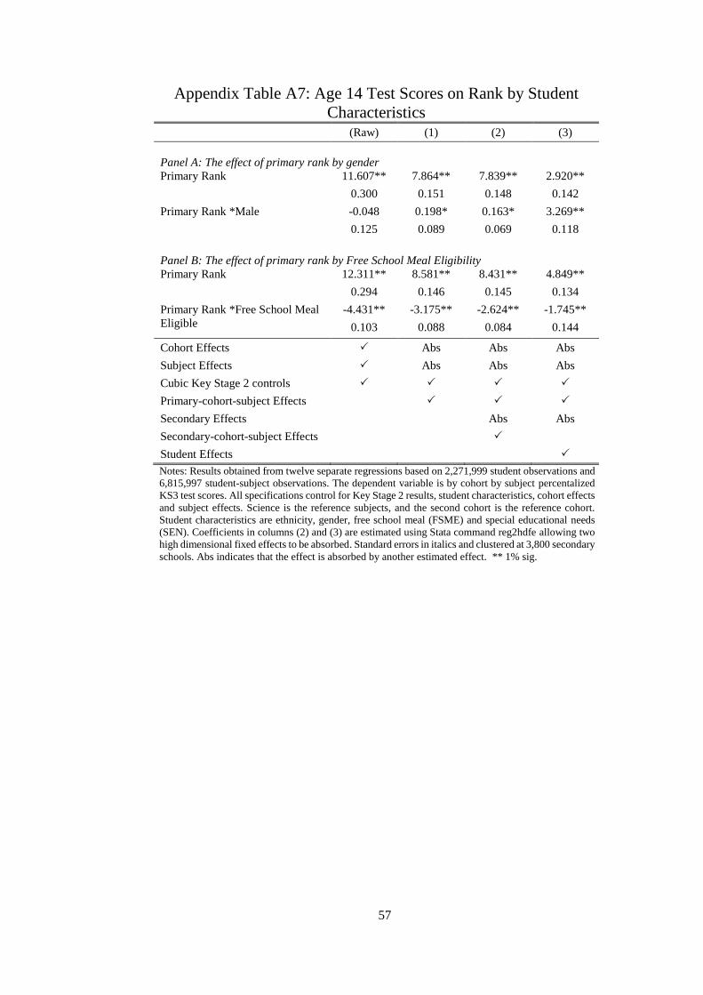
57

Appendix Table A7: Age 14 Test Scores on Rank by Student

Characteristics (Raw) (1) (2) (3)

Panel A: The effect of primary rank by gender Primary Rank 11.607** 7.864** 7.839** 2.920**

0.300 0.151 0.148 0.142

Primary Rank *Male -0.048 0.198* 0.163* 3.269**

0.125 0.089 0.069 0.118

Panel B: The effect of primary rank by Free School Meal Eligibility

Primary Rank 12.311** 8.581** 8.431** 4.849**

0.294 0.146 0.145 0.134

Primary Rank *Free School Meal

Eligible

-4.431** -3.175** -2.624** -1.745**

0.103 0.088 0.084 0.144

Cohort Effects Abs Abs Abs

Subject Effects Abs Abs Abs

Cubic Key Stage 2 controls

Primary-cohort-subject Effects

Secondary Effects Abs Abs

Secondary-cohort-subject Effects

Student Effects

Notes: Results obtained from twelve separate regressions based on 2,271,999 student observations and

6,815,997 student-subject observations. The dependent variable is by cohort by subject percentalized

KS3 test scores. All specifications control for Key Stage 2 results, student characteristics, cohort effects

and subject effects. Science is the reference subjects, and the second cohort is the reference cohort.

Student characteristics are ethnicity, gender, free school meal (FSME) and special educational needs

(SEN). Coefficients in columns (2) and (3) are estimated using Stata command reg2hdfe allowing two

high dimensional fixed effects to be absorbed. Standard errors in italics and clustered at 3,800 secondary

schools. Abs indicates that the effect is absorbed by another estimated effect. ** 1% sig.

58

Appendix 3: Education Production Function Foundation to

Empirical Specification

We use the standard education production function approach to derive a rank-augmented

value added specification that can be used to identify the effect of primary school rank,

measured as outlined in section 4.2, on subsequent outcomes.

To begin, we consider a basic contemporaneous education production function, using the

framework as set out in Todd and Wolpin (2003), for student i studying subject s in primary

school j, cohort c and in time period 𝑡 = [1,2]:

𝑌𝑖𝑗𝑠𝑐𝑡 = 𝑋𝑖′𝛽 + 𝑣𝑖𝑗𝑠𝑐𝑡 (28)

𝑣𝑖𝑗𝑠𝑐𝑡 = 𝜇𝑗𝑠𝑐 + 𝜏𝑖 + 휀𝑖𝑗𝑠𝑐𝑡

where Y denotes national academic percentile rank in subject s at time t and is determined

by X a vector of observable non-time varying characteristics of the student and 𝑣 representing

the unobservable factors. Here 𝛽 represents the permanent impact of these non-time varying

observable characteristics on academic achievement. There are two time periods, in period

one students attend primary school and in the second period students attend secondary schools.

The error term 𝑣𝑖𝑗𝑠𝑐𝑡 has three components; 𝜇𝑗𝑠𝑐 represents the permanent unobserved effects

of being taught subject j in primary school s in cohort c. This could reflect the effect of a

teacher being particularly good at teaching maths in one year but not English, or that a

student’s peers were good in English but not in science; 𝜏𝑖 represents permanent unobserved

student characteristics, this would include any stable parental inputs or natural ability of the

child; 휀𝑖𝑗𝑠𝑐𝑡 is the idiosyncratic time specific error which includes secondary school effects.

Under this restrictive specification only 휀𝑖𝑗𝑠𝑐𝑡 could cause the national academic rank of a

student to change between primary and secondary school, as all other factors are permanent

and have the same impact over time.

This is a restrictive assumption, as the impact of observable and unobservable

characteristics are likely to change as the student ages. One could imagine that neighbourhood

effects may grow in importance as the child grows older, and that the effects of primary school

are more important when the child is young and attending that school. Therefore we extend

the model by allow for time-varying effects of these characteristics:

𝑌𝑖𝑗𝑠𝑐𝑡 = 𝛽𝑅𝑎𝑛𝑘 𝑡𝑅𝑖𝑗𝑠𝑐 + 𝑋𝑖′𝛽 + 𝑋𝑖

′𝛽𝑡 + 𝑣𝑖𝑗𝑠𝑐 (29)

𝑣𝑖𝑗𝑠𝑐 = 𝜇𝑗𝑠𝑐 + 𝜇𝑗𝑠𝑐𝑡 + 𝜏𝑖 + 𝜏𝑖𝑡 + 휀𝑖𝑗𝑠𝑐

where 𝛽𝑡 allows for the effect of student characteristics to vary over time. We have also

introduced the parameter of interest 𝛽𝑅𝑎𝑛𝑘 𝑡, which is the effect of having rank 𝑅𝑖𝑗𝑠𝑐, in subject

s in cohort c and in primary school j on student achievement in that subject in the subsequent

period t. As we are interested in longer-run effects of rank positions students had during early

59

education stages, we therefore assume that there is no effect of rank in the first period t=1 as

there is no prior rank 𝛽𝑅𝑎𝑛𝑘 1 = 0. We will hence be estimating 𝛽𝑅𝑎𝑛𝑘 2, the effect of primary

school rank on period 2 outcomes. To simplify the notation the time subscript will be dropped,

as only one rank parameter is estimated, 𝛽𝑅𝑎𝑛𝑘.

This specification also allows for the unobservables to have time varying effects. Again 𝜏𝑖

represents unobserved individual effects that capture all time constant effects of a student over

time and 𝜇𝑗𝑠𝑐 represents the permanent effects of being taught in a specific school-subject-

cohort. Now additionally we have 𝜏𝑖𝑡 and 𝜇𝑗𝑠𝑐𝑡 allowing for these error components to vary

over time so that students can have individual-specific growth rates as they grow older, or that

primary school teachers can affect the efficiency of their students to learn a certain subject in

the future.

Given this structure we now state explicitly the conditional impendence assumption that

needs to be satisfied for estimating an unbiased rank parameter. Conditional on student

characteristics, time varying and permanent primary school-subject-cohort level and

individual effects, we assume there would be no expected differences in students’ outcomes

except those driven by rank.

𝑌𝑅𝑖 ⊥ 𝑅𝑖| 𝑋𝑖 , 𝜇𝑗𝑠𝑐 , 𝜇𝑗𝑠𝑐𝑡 , 𝜏𝑖, 𝜏𝑖𝑡 for all R (30)

To achieve this we require measures of all factors that may be correlated with rank and

final outcomes. Conditioning on prior test scores will absorb all non-time varying effects as

they will effect period-1 test scores to the same extent as period-2 test scores. Any input,

observable or unobservable, that would affect academic attainment is captured in these test

scores.39 Therefore we can express period two outcomes, age 14 test scores, as a function of

rank, prior test scores, student characteristics and unobservable effects.

𝑌𝑖𝑗𝑘𝑠𝑐2 = 𝛽𝑅𝑎𝑛𝑘𝑅𝑖𝑗𝑠𝑐 + 𝑓 (𝑌𝑖𝑗𝑠𝑐1(𝑋𝑖′𝛽, 𝑋𝑖

′𝛽1, 𝜏𝑖 , 𝜇𝑗𝑠𝑐 , 𝜏𝑖1, 𝜇𝑗𝑠𝑐1)) +

+𝑋𝑖′𝛽2 + 𝜇𝑗𝑠𝑐2 + 𝜏𝑖2 + 𝜖𝑖𝑗𝑘𝑠𝑐 (31)

Using lagged test scores means that the remaining factors are those that affect the learning

in period 2, between ages 11 and 14 (𝑋𝑖′𝛽𝑡, 𝜇𝑗𝑠𝑐2, 𝜏𝑖2). In our regressions, we will allow the

functional form of this lagged dependent variable to take two forms, either a 3rd degree

polynomial or a fully flexible measure, which allows for a different effect at each national test

score percentile. As we can observe certain characteristics and primary school attended, 𝛽2

and 𝜇𝑗𝑠𝑐2 can easily be estimated. The interpretation of 𝜇𝑗𝑠𝑐2 is that some primary schools are

more effective at teaching for a later test than others, in a way that does not show up in the

end-of-primary age-11 test scores.

39 Examples of these effects include students’ innate ability, parental investment, teacher effects, peer

effects and primary school infrastructure

60

The discussion of recovering 𝜏𝑖2, the second period academic growth of individual i is

below, but it is worth spending some time interpreting what the rank coefficient represents

without its inclusion. Being ranked highly in primary school may have positive spillover effect

in other subjects. Any estimation, which allows for individual growth rates during secondary

school (second period), would absorb any spillover effects. Therefore, leaving 𝜏𝑖2 in the

residual means that the rank parameter is the effect of rank of the subject in question and the

correlation in rank from the other two subjects, as we have test scores for English, mathematics

and science.

In the second period the student will be attending secondary school k which may affect

later test scores by subject, 𝜋𝑘𝑠𝑐, which is another component of the error term 𝜖𝑖𝑗𝑘𝑠𝑐, where

𝜖𝑖𝑗𝑘𝑠𝑐 = 𝜋𝑘𝑠𝑐 + 휀𝑖𝑗𝑘𝑠𝑐 . As stated above conditional on time-varying student effects, prior

subject test scores and the other stated factors, we do not expect that these components will

be correlated with primary rank. This is primarily because general secondary school effects

are absorbed by the time varying student effect..

The first two specifications that we estimate that will recover the effect of rank due to

overall changes in effort which allow for spill-overs between subjects, are the following:

𝑌𝑖𝑗𝑘𝑠𝑐2 = 𝛽𝑅𝑎𝑛𝑘𝑅𝑖𝑗𝑠𝑐 + 𝑓(𝑌𝑖𝑗𝑠𝑐1) + 𝑋𝑖′𝛽2 + 𝜇𝑗𝑠𝑐2 + 𝜖𝑖𝑗𝑘𝑠𝑐 (32)

Where 𝜖𝑖𝑗𝑘𝑠𝑐 = 𝜏𝑖2 + 𝜋𝑘𝑠𝑐 + 휀𝑖𝑗𝑘𝑠𝑐

𝑌𝑖𝑗𝑘𝑠𝑐2 = 𝛽𝑅𝑎𝑛𝑘𝑅𝑖𝑗𝑠𝑐 + 𝑓(𝑌𝑖𝑗𝑠𝑐1) + 𝑋𝑖′𝛽2 + 𝜇𝑗𝑠𝑐2 + 𝜋𝑘𝑠𝑐 + 𝜓𝑖𝑗𝑘𝑠𝑐 (33)

Where 𝜓𝑖𝑗𝑘𝑠𝑐 = 𝜏𝑖2 + 휀𝑖𝑗𝑘𝑠𝑐

We now further augment these regressions by including the average student growth rate

across subjects to recover individual growth effects, 𝜏𝑖2. Note that despite using panel data,

this is estimating the individual effect across subjects and not over time. Lavy (et al. 2012)

also use a student-fixed effects strategy to estimate ability peer effects. Applied to this setting,

when allowing for student effects, we effectively compare relative rankings within an

individual, controlling for national subject-specific ability. The variation used to identify rank

is correlation between the differential growth rates by subject within each student and prior

subject ranking. Therefore any individual characteristic that is not realised in age-11 test

scores but contributes towards age-14 test scores is accounted for, including secondary school

attended, as long as the effects are not subject specific.

𝑌𝑖𝑗𝑘𝑠𝑐2 = 𝛼𝑡 + 𝛽𝑅𝑎𝑛𝑘𝑅𝑖𝑗𝑠𝑐 + 𝑓(𝑌𝑖𝑗𝑠𝑐1) + 𝜏𝑖2 + 𝜇𝑗𝑠𝑐2 + 𝜖𝑖𝑗𝑘𝑠𝑐 (34)

Where 𝜖𝑖𝑗𝑘𝑠𝑐 = 𝜋𝑘𝑠𝑐 + 휀𝑖𝑗𝑘𝑠𝑐

In these specifications the rank parameter only represents the increase in test scores due to

subject specific rank, as any general gains across all subjects would be absorbed by the student

effect. This can be interpreted as the extent of specialisation in subject s due to primary school

rank. It is for this reason, and the removal of other covarying factors, why we would expect

61

the coefficient of the rank effect in specification (34) to be smaller than those found in (32) or

(33).

Finally, to also investigate potential non-linearites in the effect of ordinal rank on later

outcomes, i.e. are effects driven by students being top or bottom of the class, we replace the

linear ranking parameter with indicator variables according to quantiles in rank plus additional

indicator variables for those at the top and bottom of each school-subject-cohort (the rank

measure is defined in section 4.2). We allow for non-linear effects according to vingtiles in

rank, which can be applied to all the specifications presented. 40

𝑌𝑖𝑗𝑘𝑠𝑐2 = 𝛽𝑅=0𝐵𝑜𝑡𝑡𝑜𝑚𝑖𝑗𝑠𝑘 + ∑ 𝐼𝑛𝑅𝑖𝑗𝑠𝑐

20

𝑛=1

𝛽𝑛,𝑅𝑎𝑛𝑘 + 𝛽𝑅=1𝑇𝑜𝑝𝑖𝑗𝑠𝑐

+ 𝑓(𝑌𝑖𝑗𝑠𝑐1) + 𝜏𝑖 + 𝜇𝑗𝑠𝑐 + 𝜖𝑖𝑗𝑘𝑠𝑐 (35)

In summary, if students react to ordinal information as well as cardinal informaiton, then

we would expect the rank in adition to relative achivement to have a signficant effect on later

achievement when estimating these equations. This is what is picked up by the 𝛽𝑅𝑎𝑛𝑘 -

coefficient. The following sections discuss potential threats to identification, the setting, and

how rank is measured before we turn to the estimates.

40 Estimates are robust to using deciles in rank rather than vigntiles and can be obtained upon request.