Introduction

• We have dealt with polylines and mesh shapes.

• We want a way to describe curved shapes which will make them easy to draw.

Example: Animation

• The path of the camera through the scene must be specified at each instant.

• The camera is located on the path P(t) at time t.

tree

pond

road

x

y

@ t = 0 @ 5

@ 2

@ 1

house

P(t)

Animation (2)

• The designer chooses a suitable function P(t) so that the camera moves as desired, perhaps taking snapshot #1 at t = 0.1, snapshot #2 at t = 0.2, etc.

• The view direction of the camera must also be specified at each instant.

tree

pond

road

x

y

@ t = 0 @ 5

@ 2

@ 1

house

P(t)

Animation (3)

• The camera must move smoothly along P(t) without any disturbing jerks. – This imposes conditions on the velocity P’(t).

• Other objects might move as well: the car, the boat, and any people coming out of the house.

• The movement of each of these objects must be described by specifying appropriate parametric functions F(t), G(t), etc.

Smoothness of Motion

• The velocity v(t) is a vector that describes the speed and direction of an object moving along P(t) as it traverses the curve.

• It is given by

dt

dy

dt

dx

dt

tdPv ,

)(

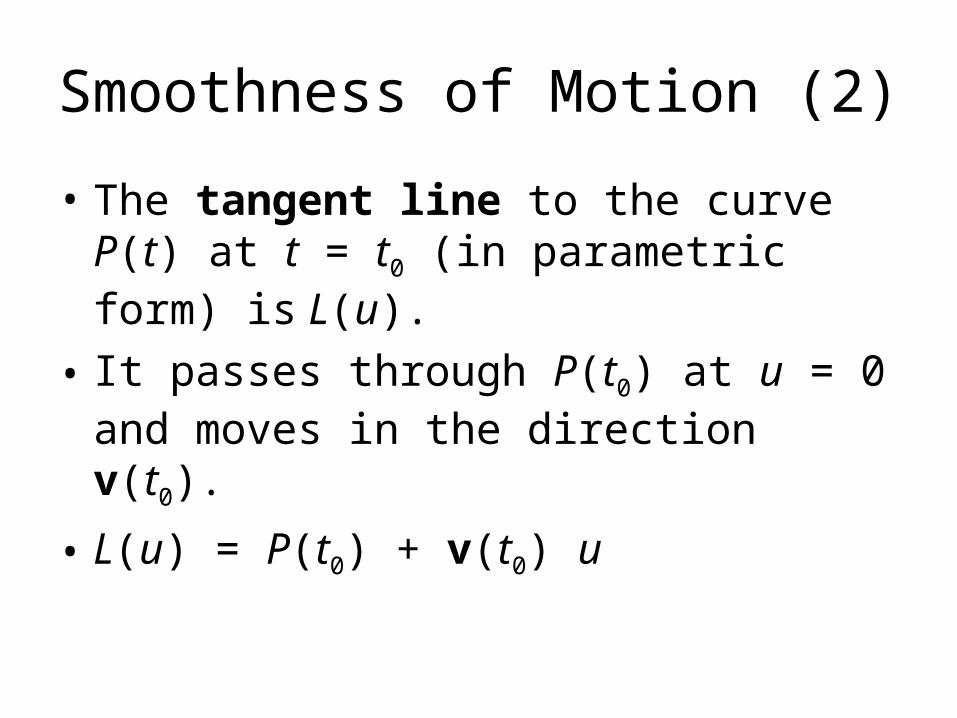
Smoothness of Motion (2)

• The tangent line to the curve P(t) at t = t0 (in parametric form) is L(u).

• It passes through P(t0) at u = 0 and moves in the direction v(t0).

• L(u) = P(t0) + v(t0) u

Smoothness of Motion (3)

• The normal direction to a curve may be found at each point.

• It is defined as the direction perpendicular to the tangent line at the point.

• If the tangent line has direction v(t0) at time t0, the normal direction at t0 is any multiple of the vector– n(t0) = v┴( t0) = (-dy/dt, dx/dt)|t = t0

Example: Motion on an Ellipse

• The figure shows velocities along an ellipse.

• What happens if, at t = a, the speed increases by a factor of 3?

x

y

v(t)P(t)

Motion along an Ellipse (2)

• The trajectory is an ellipse; at t = a both x(t) and y(t) start to oscillate 3 times faster.

• Their derivatives at t = a are discontinuous.

• The shape of the curve is the same, but the motion changes.

t

t

y(t)

x(t)a

a

y

x

Parametric Continuity

• We say a curve P(t) has k-th order parametric continuity everywhere in the t-interval [a, b] if all derivatives of the curve, up through the k-th, exist and are continuous at all points inside [a, b].

• Briefly, P( ) is k-smooth in [a, b].

• We insist on at least 1-smooth curves for animation, to avoid jerky motion.

Visual Smoothness

• A curve in an interval is 0-smooth if it is continuous.

• A curve is 1-smooth if its first derivative exists and is continuous throughout the interval.

• A curve is 2-smooth if its first and second derivatives exist and are continuous throughout the interval.

• A curve is 3-smooth if its first, second, and third derivatives exist and are continuous throughout the interval. – A 3-smooth curve must also be 2-smooth, but a 2-

smooth curve may or may not be 3-smooth.

Geometric Continuity (Gk-continuity).

• G0 continuity is the same as 0-smoothness: P(t) is continuous with respect to t throughout [a, b].

• G1 continuity in [a, b] means that P’(c-) = k P'(c+) for some constant k and for every c in the interval [a,b].

• G2 continuity in [a, b] means that P’(c-) = k P’(c+) and P’’(c-) = m P’’(c+) for constants k and m and for every c in the interval [a, b].

Describing Curves by Polynomials

• A kth degree polynomial is a function given by P (t) = ak tk + ak-1 tk-1 + … + a1 t + a0.

• {ak, ak-1, …, a0} are the coefficients.

• Degree of the polynomial: highest power of t in it (i.e., k).

• Order of the polynomial: number of coefficients (i.e., k+1).

Polynomials of Degree 1

• P(t) = a0 + a1t, a linear curve (straight line). – The equation for P(t) is (in 2 dimensions) 2

equations, one for x(t) and one for y(t).– In 3 dimensions, it is 3 equations, one each

for x(t), y(t), z(t).

– P(t) passes through point a0 at t = 0, and through point a1 at t = 1.

Polynomials of Degree 2

• X(t) = at2 + bt + c, y(t) = dt2 + et + f– For any choice of a, b, c, d, e, and f, this

curve is a parabola.– We cannot generate an ellipse or a hyperbola

from this form.

• More generally, we use F(x, y) = Ax2 + 2Bxy + Cy2 + Dx + Ey +F = 0 to generate conic sections.

Polynomials of Degree 2 (cont.)

• Which conic is generated depends on the value of the discriminant, AC – B2.– If AC – B2 > 0, we generate an ellipse.– If AC – B2 = 0, we generate a parabola.– If AC – B2 < 0, we generate a hyperbola.

• Example implicit functions: – Ellipse: x2 + xy + y2 - 1: (AC-B2 = 0.75)– Parabola: x2 + 2xy + y2 + 3x – 6y – 7: (AC-B2=

0)– Hyperbola: x2 + 4xy + 2y2 -4x +y -3: (AC-B2= -

2)

Polynomials of Degree 2 (cont.)

• A special case of the general quadratic form, the common vertex equation, y2 = 2px – (1-ε2)x2, shows how the conic sections are related.– This curve passes through (0,0) and has a

size proportional to constant p. The conic that it describes depends on the value of the eccentricity ε.

– Eccentricity measures how far off the curve is from a perfect circle (eccentricity = 0).

Polynomials of Degree 2 (cont.)

= 0.8

= 1.0

= 1.5

= 0

circle

hyperbola

parabola

ellipse

x

y

p

Polynomial Curves of Degree 3 and Higher

• Polynomial curves of degree 3 and higher do not easily convert to a parametric form.

• Cubic polynomials prove very useful in curve and surface design, but start with a collection of control points provided by the designer, and use an algorithm to generate points on the curve.

• The designer may edit the positions of the control points and view the new curve.

• This approach is visual, allowing the designer to see the progress of the curve design as the process continues.

Rational Parametric Forms

• X and y are defined as the ratio of two polynomials (quadratic in the example).

• P0, P1, and P2 are any 3 points on the plane, called control points.

• W is a weight parameter.

22

221

20

121

121)(

ttwtt

tPttwPtPtP

Rational Parametric Forms (2)

• The equation for P(t) is actually 2 equations: one each for x(t) and y(t).

• P(t) is a linear combination of control points. It turns out also to be an affine combination of these points, so it makes sense as a point.

22

221

20

121

121)(

ttwtt

txttwxtxtx

22

221

20

121

121)(

ttwtt

tyttwytyty

Rational Parametric Forms (3)

• At t=0, the right hand side collapses simply to (x0, y0); this curve passes through, or interpolates, the point P0.

• At t=1, it passes through P2. For t in between 0 and 1, P(t) depends on all three points in a complicated way.

• The figure on the next slide shows the curves, which depend on the value of w.

Rational Parametric Forms (4)

P1

P0

P2

???

P1

P0

P2

hyperbola

parabola

ellipse

a). b).

Rational Parametric Forms (5)

• if w < 1 it is an ellipse

• if w = 1 it is a parabola

• if w > 1 it is a hyperbola

• Rational parametric forms provide a way to generate the conic sections parametrically.

Interactive Curve Design

• We wish to allow a designer to specify a small number of control points and draw a wide variety of curve shapes.

• The goal is to capture the shape of this curve in a form that permits it to be reproduced at will, adjusted in shape and size as desired, sent to a machine for automatic cutting or molding, etc.

• There is most likely no simple formula that matches it exactly.

Interactive Curve Design (2)

• To enter the curve, the designer moves the pointer along the curve (on a tablet) clicking at a set of control points P0, P1,... close to the curve.

P0

P1

P2

P3

a). Desired Curve b). User places points c). The algorithm generatesmany points along a "nearby" curve

desired curve

approximatingcurve

Interactive Curve Design (3)

• The role of the algorithm is to produce a point P(t) for any value of t given to it. The data for the algorithm is the set of control points, which together determine the curve along which the points P(t) will fall.

any t

P(t)P0, P1, .., PL

Control Points:curve generation algorithm

Interactive Curve Design (4)

• The algorithm is usually implemented as a function Point2 curvePt(double t, RealPointArray pts) that returns a point for any value of t in a certain interval.

• To draw the curve the user can choose a sequence of t-values, evaluate curvePt() at each of them, and connect the points with line segments to form a polyline.

Interactive Curve Design (5)

• Steps in Interactive Curve Design:– 1. Lay down the initial control points;– 2. Use the algorithm to generate the curve;– 3. If the curve is satisfactory, stop;– 4. Else, move some control points;– 5. Go to step 2;

Interpolation and Approximation

• Interpolation: curve passes through the control points (left).

• Approximation: curve passes near each control point (right).

P(t)

a). The curve interpolates the control points

b). The curve approximates the control points

R(t)

Bezier Curves

• Bezier curves (approximating curves) were developed to assist in car shape design. The de Casteljau algorithm is used to draw them.

• The de Casteljau algorithm is based on a sequence of familiar tweening steps (Chapter 5) that are easy to implement.

• Because tweening is such a well-behaved procedure, it is possible to deduce many valuable properties of the curves that it generates.

Bezier Curves (2)

• Tweening 3 points to obtain a parabola: – Start with three points: P0, P1, and P2.

– Choose t between 0 and 1, say t = 0.3. – Locate the point A that is fraction t of the way

along the line from P0 to P1. Similarly, locate B at fraction t between the endpoints P1 and P2 (using the same t).

– The new points are A(t) = (1 - t)P0 + tP1, B(t) = (1 -t)P1 + tP2

Bezier Curves (3)

• Now repeat the linear interpolation step on these points (using the same t): Find the point, P(t), that lies fraction t of the way between A and B: P(t) = (1-t)A + tB.

P0

P1

P2A

B

P at t = 0.3

a).

P0

P1

P2P(t)

P(0.3)

b).

Bezier Curves (4)

• If this process is carried out for every t between 0 and 1, the curve P(t) will be generated.

• The parametric form for this curve is P(t) = (1-t)2P0 + 2t(1-t)P1 + t2P2

Bezier Curves (5)

• The parametric form for P(t) is quadratic in t, so we know the curve is a parabola.

• It will still be a parabola even if t is allowed to vary from –∞ to ∞.

• It passes through P0 at t = 0 and through P2 at t = 1 (why?)

• We thus have a well-defined process that can generate a smooth parabolic curve based on three given points.

Bezier Curves (6)

• The most common Bezier curves use 4 control points. • For a given value of t, point A is placed fraction t of the

way from P0 to P1, and similarly for points B and C. • Then D is placed fraction t of the way from A to B, and

similarly for point E. • Finally, the desired point P is located fraction t of the way

from D to E.

P0

P1

P2

PP3A

BC

D

E

a). b).

Bezier Curves (7)

• If this is done for every t between 0 and 1, the curve P(t) starts at P0, is attracted toward P1 and P2, and ends at P3.

• It is the Bezier curve determined by the four points.

Bezier Curves (8)

• The Bezier curve based on four points has the parametric form P(t) = P0(1-t)3 + P13(1-t)2t + P23(1-t)t2 + P3t3.

• Each control point Pi is weighted by a cubic polynomial, and the weighted terms are added.

• The terms involved here are known as Bernstein polynomials.

Bernstein Polynomials

• The Bernstein polynomials are

• These polynomials add to 1 for any value of t. [In fact, they are the expansion of (1 – t + t)3.]

• Consequently, P(t) is an affine combination of points, and thus a legitimate point.

330 1 tB ttB 23

1 13 232 13 ttB 33

3 tB

Bernstein Polynomials (2)

t1

1B (t)

3

0 B (t)3

1 B (t)3

2

B (t)3

3

Blending Points with Bernstein Polynomials

• The points are vectors bound to the origin (e.g., P0 = po, etc.) and t = 0.3. Then p(0.3) = 0.343 p0 + 0.441 p1 + 0.189 p2 + 0.027 p3.

• In the figure the four vectors are weighted and the results are added using the parallelogram rule to form the vector p(0.3).

Generalizing Bezier Curves to Any Number of Points

• For each value of t, a succession of generations are built up, each by tweening adjacent points produced in the previous generation (superscript for P is the generation number):

Pi4( t) (1 t)Pi

3( t) tPi13 (t)

PiL(t) (1 t)Pi

L 1(t) tPi1L 1(t) for i = 0, . . . , L .

Generalizing Bezier Curves to Any Number of Points (2)

• The resulting curve is

• For L ≥ k, the binomial coefficient is

• For L< k, the binomial coefficient is 0.

P(t) Pk kLB (t)

k0

L

kkLL

k ttk

LtB

)1()(

!!

!

kLk

L

k

L

Properties of Bezier Curves

• Bezier curves have properties well-suited to CAD. – Endpoint Interpolation: The Bezier curve P(t) based

on control points P0, P1, . . ., PL always interpolates P0 and PL.

– Affine Invariance: to apply an affine transformation T to all points P(t) on the Bezier curve, we transform the control points (once), and use the new control points to re-create the transformed Bezier curve Q(t) at any t.

– )()()(0

tBPTtQL

k

Lkk

Properties of Bezier Curves (2)

– Example: A Bezier curve based on four control points P0,..., P3. The points are rotated, scaled, and translated to the new control points Qk.

– The Bezier curve for Qk is drawn. It is identical to the result of transforming the original Bezier curve.

Q0 Q2

Q1

P2

P0

Q3

P3

P1

Properties of Bezier Curves (3)

– Convex Hull Property: a Bezier curve, P(t), never wanders outside its convex hull.

– The convex hull of a set of points P0, P1, . . ., PL is the set of all convex combinations of the points; that is, the set of all points given by

where each αk is non-negative, and they sum to 1.

k

L

kkP

0

Properties of Bezier Curves (4)

• Example: Even though the eight control points form a jagged control polygon, the designer knows the Bezier curve will flow smoothly between the two endpoints, never extending outside the convex hull.

Properties of Bezier Curves (5)

• Derivatives of Bezier Curves: the first derivative is

where ΔPk = Pk+1 - Pk • The velocity is another Bezier curve, built on a

new set of control vectors ΔPk . • Taking the derivative lowers the order of the

curve by 1: the derivative of a cubic Bezier curve is a quadratic Bezier curve.

)()( 11

0

' tBPLtp Lk

L

kk

Drawing Bezier Curves

• Complete code for drawing Bezier curves is in Fig. 10.18.